Statistical Inference for Generative Models
with Maximum Mean Discrepancy

François-Xavier Briol1,3 Alessandro Barp2,3 Andrew B. Duncan2,3 Mark Girolami1,3
1University of Cambridge
Department of Engineering
2Imperial College London
Department of Mathematics
3The Alan Turing Institute
Abstract

While likelihood-based inference and its variants provide a statistically efficient and widely applicable approach to parametric inference, their application to models involving intractable likelihoods poses challenges. In this work, we study a class of minimum distance estimators for intractable generative models, that is, statistical models for which the likelihood is intractable, but simulation is cheap. The distance considered, maximum mean discrepancy (MMD), is defined through the embedding of probability measures into a reproducing kernel Hilbert space. We study the theoretical properties of these estimators, showing that they are consistent, asymptotically normal and robust to model misspecification. A main advantage of these estimators is the flexibility offered by the choice of kernel, which can be used to trade-off statistical efficiency and robustness. On the algorithmic side, we study the geometry induced by MMD on the parameter space and use this to introduce a novel natural gradient descent-like algorithm for efficient implementation of these estimators. We illustrate the relevance of our theoretical results on several classes of models including a discrete-time latent Markov process and two multivariate stochastic differential equation models.

1 Introduction

Consider an open subset π’³βŠ‚β„d𝒳superscriptℝ𝑑\mathcal{X}\subset\mathbb{R}^{d} and denote by 𝒫​(𝒳)𝒫𝒳\mathcal{P}(\mathcal{X}) the set of Borel probability measures on this domain. We consider the problem of learning a probability measure β„šβˆˆπ’«β€‹(𝒳)β„šπ’«π’³\mathbb{Q}\in\mathcal{P}(\mathcal{X}) from identically and independently distributed (IID) realisations {yj}j=1mβ€‹βˆΌIIDβ„šsuperscriptsubscriptsubscript𝑦𝑗𝑗1π‘šIIDsimilar-toβ„š\{y_{j}\}_{j=1}^{m}\operatorname*{\overset{\scriptscriptstyle\text{IID}}{\scriptscriptstyle\sim}}\mathbb{Q}. We will focus on parametric inference with a parametrised family π’«Ξ˜β€‹(𝒳)={β„™ΞΈβˆˆπ’«β€‹(𝒳):θ∈Θ}subscriptπ’«Ξ˜π’³conditional-setsubscriptβ„™πœƒπ’«π’³πœƒΞ˜\mathcal{P}_{\Theta}(\mathcal{X})=\{\mathbb{P}_{\theta}\in\mathcal{P}(\mathcal{X})\,:\,\theta\in\Theta\}, for an open set Ξ˜βŠ‚β„pΘsuperscriptℝ𝑝\Theta\subset\mathbb{R}^{p} i.e. we seek ΞΈβˆ—βˆˆΞ˜superscriptπœƒΞ˜\theta^{*}\in\Theta such that β„™ΞΈβˆ—subscriptβ„™superscriptπœƒ\mathbb{P}_{\theta^{*}} is closest to β„šβ„š\mathbb{Q} in an appropriate sense. If β„šβˆˆπ’«Ξ˜β€‹(𝒳)β„šsubscriptπ’«Ξ˜π’³\mathbb{Q}\in\mathcal{P}_{\Theta}(\mathcal{X}) we are in the M-closed setting, otherwise we are in the M-open setting. When β„™ΞΈsubscriptβ„™πœƒ\mathbb{P}_{\theta} has a density p(β‹…|ΞΈ)p(\cdot|\theta) with respect to the Lebesgue measure, then a standard approach is to use the maximum likelihood estimator (MLE):

ΞΈ^mMLEsuperscriptsubscript^πœƒπ‘šMLE\displaystyle\hat{\theta}_{m}^{\text{MLE}} =arg​maxθ∈Θ⁑1mβ€‹βˆ‘j=1mlog⁑p​(yj|ΞΈ).absentsubscriptargmaxπœƒΞ˜1π‘šsuperscriptsubscript𝑗1π‘šπ‘conditionalsubscriptπ‘¦π‘—πœƒ\displaystyle=\operatorname*{arg\,max}_{\theta\in\Theta}\frac{1}{m}\sum_{j=1}^{m}\log p(y_{j}|\theta).

For complex models, a density may not be easily computable, or even exist and so the MLE need not be available. In some cases it is possible to approximate the likelihood; see for example pseudo likelihood (Besag, 1974), profile likelihood (Murphy and van der Vaart, 2000) and composite likelihood (Varin etΒ al., 2011) estimation. It is sometimes also possible to access likelihoods in un-normalised forms i.e. p​(y|ΞΈ)=p¯​(y|ΞΈ)/C​(ΞΈ)𝑝conditionalπ‘¦πœƒΒ―π‘conditionalπ‘¦πœƒπΆπœƒp(y|\theta)=\bar{p}(y|\theta)/C(\theta) where the constant C​(ΞΈ)πΆπœƒC(\theta) is unknown. This class of models is known as un-normalised models, or doubly-intractable models in the Bayesian literature, and a range of exact and approximate methods have been developped for this case; see for example the Markov chain Monte Carlo (MCMC) algorithms of Murray etΒ al. (2006); Moller etΒ al. (2006) or the score-based and ratio-based approaches of HyvΓ€rinen (2006, 2007); Gutmann and Hyvarinen (2012).

However, for many models of interest in modern statistical inference, none of the methods above can be applied straightforwardly and efficiently due to the complexity of the likelihoods involved. This is most notably the case for intractable generative models, sometimes also called implicit models or likelihood-free models; see Mohamed and Lakshminarayanan (2016) for a recent overview. Intractable generative models are parametric families of probability measures for which it is possible to obtain realisations for any value of the parameter ΞΈβˆˆΞ˜πœƒΞ˜\theta\in\Theta, but for which we do not necessarily have access to a likelihood or approximation thereof. These models are used throughout the sciences, including in the fields of ecology (Wood, 2010), population genetics (Beaumont etΒ al., 2002) or astronomy (Cameron and Pettitt, 2012). They also appear in machine learning as black-box models; see for example generative adversarial networks (GANs) (Goodfellow etΒ al., 2014) and variational auto-encoders (Kingma and Welling, 2014).

Given a Borel probability space (𝒰,β„±,π•Œ)π’°β„±π•Œ(\mathcal{U},\mathcal{F},\mathbb{U}), we will call generative model any probability measure which is the pushforward GΞΈ#β€‹π•ŒsuperscriptsubscriptπΊπœƒ#π•ŒG_{\theta}^{\#}\mathbb{U} of the probability measure π•Œπ•Œ\mathbb{U} with respect to a measurable parametric map GΞΈ:𝒰→𝒳:subscriptπΊπœƒβ†’π’°π’³G_{\theta}:\mathcal{U}\rightarrow\mathcal{X} called the generator. To generate n𝑛n independent realisations from the model, we produce IID realisations {ui}i=1nβ€‹βˆΌIIDπ•Œsuperscriptsubscriptsubscript𝑒𝑖𝑖1𝑛IIDsimilar-toπ•Œ\{u_{i}\}_{i=1}^{n}\operatorname*{\overset{\scriptscriptstyle\text{IID}}{\scriptscriptstyle\sim}}\mathbb{U} and apply the generator to each of these samples: xi=Gθ​(ui)subscriptπ‘₯𝑖subscriptπΊπœƒsubscript𝑒𝑖x_{i}=G_{\theta}(u_{i}) for i=1,…,n𝑖1…𝑛i=1,\ldots,n. While it is straightforward to generate samples from these models, a likelihood function need not be available, given that an associated positive density may not be computable or even exist. We therefore require alternatives to the MLE.

The estimators studied in this paper fall within the class of minimum divergence/distance estimators (Pardo, 2005; Basu etΒ al., 2011). These are estimators minimising some notion of divergence D:𝒫​(𝒳)×𝒫​(𝒳)→ℝ+:𝐷→𝒫𝒳𝒫𝒳subscriptℝD:\mathcal{P}(\mathcal{X})\times\mathcal{P}(\mathcal{X})\rightarrow\mathbb{R}_{+} (or an approximation thereof) between an empirical measure β„šm=1mβ€‹βˆ‘j=1mΞ΄yjsuperscriptβ„šπ‘š1π‘šsuperscriptsubscript𝑗1π‘šsubscript𝛿subscript𝑦𝑗\mathbb{Q}^{m}=\frac{1}{m}\sum_{j=1}^{m}\delta_{y_{j}} (where Ξ΄yjsubscript𝛿subscript𝑦𝑗\delta_{y_{j}} denotes a Dirac measure at yjsubscript𝑦𝑗y_{j}), obtained from the data {yj}j=1mβ€‹βˆΌIIDβ„šsubscriptsuperscriptsubscriptπ‘¦π‘—π‘šπ‘—1IIDsimilar-toβ„š\{y_{j}\}^{m}_{j=1}\operatorname*{\overset{\scriptscriptstyle\text{IID}}{\scriptscriptstyle\sim}}\mathbb{Q}, and the parametric model:

ΞΈ^mDsubscriptsuperscript^πœƒπ·π‘š\displaystyle\hat{\theta}^{D}_{m} =argminθ∈ΘD(β„™ΞΈ||β„šm)\displaystyle=\operatorname*{argmin}_{\theta\in\Theta}D(\mathbb{P}_{\theta}||\mathbb{Q}^{m}) (1)

If β„šmsuperscriptβ„šπ‘š\mathbb{Q}^{m} was absolutely continuous with respect to β„™ΞΈsubscriptβ„™πœƒ\mathbb{P}_{\theta}, maximising the likelihood would correspond to minimising the Kullback-Leibler (KL) divergence which, given β„™1,β„™2βˆˆπ’«β€‹(𝒳)subscriptβ„™1subscriptβ„™2𝒫𝒳\mathbb{P}_{1},\mathbb{P}_{2}\in\mathcal{P}(\mathcal{X}), is defined as DKL(β„™1||β„™2):=βˆ«π’³log(dβ„™1/dβ„™2)dβ„™1D_{\text{KL}}(\mathbb{P}_{1}||\mathbb{P}_{2}):=\int_{\mathcal{X}}\log(\mathrm{d}\mathbb{P}_{1}/\mathrm{d}\mathbb{P}_{2})\mathrm{d}\mathbb{P}_{1}, where d​ℙ1/d​ℙ2dsubscriptβ„™1dsubscriptβ„™2\mathrm{d}\mathbb{P}_{1}/\mathrm{d}\mathbb{P}_{2} is the Radon-Nikodym derivative of β„™1subscriptβ„™1\mathbb{P}_{1} with respect to β„™2subscriptβ„™2\mathbb{P}_{2}. This approach to inference is useful for models with complicated or intractable likelihood, since the choice of divergence can be adapted to the class of models of interest.

In previous works, minimum distance estimators for generative models have been considered based on the Wasserstein distance and its Sinkhorn relaxation; see Bassetti etΒ al. (2006); Frogner etΒ al. (2015); Montavon etΒ al. (2016); Genevay etΒ al. (2018); Frogner and Poggio (2018); Sanjabi etΒ al. (2018). These have the advantage that they can leverage extensive work in the field of optimal transport. In a Bayesian context, similar ideas are used in approximate Bayesian computation (ABC) methods Marin etΒ al. (2012); Lintusaari etΒ al. (2017) where synthetic data sets are simulated from the model then compared to the true data using some notion of distance. There, significant work has been put into automating the choice of distance (Fearnhead and Prangle, 2011), and the use of the Wasserstein distance has also recently been studied (Bernton etΒ al., 2019).

In this paper, we shall investigate the properties of minimal divergence estimators based on an approximation of maximum mean discrepancy (MMD). Such estimators have already been used extensively in the machine learning literature with generators taking the form of neural networks (Dziugaite etΒ al., 2015; Li etΒ al., 2015, 2017; Sutherland etΒ al., 2017; Arbel etΒ al., 2018; BiΕ„kowski etΒ al., 2018; Romano etΒ al., 2018; dos Santos etΒ al., 2019) where they are usually called MMD GANs, but can be used more generally. Our main objective in this paper is to present a general framework for minimum MMD estimators, to study their theoretical properties and to provide an initial discussion of the impact of the choice of kernel. This study brings insights into the favourable empirical results of previous work in MMD for neural networks, and demonstrate more broadly the usefulness of this approach for inference within the large class of intractable generative models of interest in the statistics literature. As will be discussed, this approach is significantly preferable to alternatives based on the Wasserstein distance for models with expensive generators as it comes with significantly stronger generalisation bounds and is more robust in several scenarios. Our detailed contributions can be summarised as follows:

  1. 1.

    In Section 2, we introduce the MMD metric, minimum MMD estimators, and the statistical Riemannian geometry the metric induces on the parameter space ΘΘ\Theta. Through this, we rephrase the mimimum divergence estimator problem in terms of a gradient flow, thus obtaining a stochastic natural gradient descent method for finding the estimator ΞΈβˆ—superscriptπœƒ\theta^{*} which can significantly reduce computation cost as compared to stochastic gradient descent.

  2. 2.

    In Section 3, we focus on the theoretical properties of minimum MMD estimators and associated approximations. We use the information geometry of MMD to demonstrate generalisation bounds and statistical consistency, then prove that the estimator is asymptotically normal in the M-closed setting. These results give us necessary assumptions on the generator for the use of the estimators. We then analyse the robustness properties of the estimator in the M-open setting, establishing conditions for qualitative and quantitative robustness.

  3. 3.

    In Section 4 we study the efficiency and robustness of minimum MMD estimators based on Gaussian kernels for classes of isotropic Gaussian location and scale models. We demonstrate the effect of the kernel lengthscale on the efficiency of the estimators, and demonstrate a tradeoff between (asymptotic) efficiency and robustness. For high-dimensional problems, we demonstate that choosing the lengthscale according to the median heuristic provides an asymptotic variance independent of dimensionality. We also extend our analysis to mixtures of kernels, providing insights on settings often considered in machine learning applications.

  4. 4.

    In Section 5, we perform numerical simulations to support the theory detailed in the previous sections, demonstrating the behaviour of minimum MMD estimators for a number of examples including estimation of unknown parameters for the g-and-k distribution, in a stochastic volatility model and for two systems of stochastic differential equations.

2 The Maximum Mean Discrepancy Statistical Manifold

We begin by formalising the notion of MMD and introduce the corresponding minimum MMD estimators. We then use tools from information geometry to analyse these estimators, which leads to a stochastic natural gradient descent algorithm for efficient implementation.

2.1 Maximum Mean Discrepancy

Let k:𝒳×𝒳→ℝ:π‘˜β†’π’³π’³β„k:\mathcal{X}\times\mathcal{X}\rightarrow\mathbb{R} be a Borel measurable kernel on 𝒳𝒳\mathcal{X}, and consider the reproducing kernel Hilbert space β„‹ksubscriptβ„‹π‘˜\mathcal{H}_{k} associated with kπ‘˜k (see Berlinet and Thomas-Agnan (2004)), equipped with inner product βŸ¨β‹…,β‹…βŸ©β„‹ksubscriptβ‹…β‹…subscriptβ„‹π‘˜\langle\cdot,\cdot\rangle_{\mathcal{H}_{k}} and norm βˆ₯β‹…βˆ₯β„‹ksubscriptdelimited-βˆ₯βˆ₯β‹…subscriptβ„‹π‘˜\lVert\cdot\rVert_{\mathcal{H}_{k}}. Let 𝒫k​(𝒳)subscriptπ’«π‘˜π’³\mathcal{P}_{k}(\mathcal{X}) be the set of Borel probability measures ΞΌπœ‡\mu such that βˆ«π’³k​(x,x)​μ​(d​x)<∞subscriptπ’³π‘˜π‘₯π‘₯πœ‡dπ‘₯\int_{\mathcal{X}}\sqrt{k(x,x)}\mu(\mathrm{d}x)<\infty. The kernel mean embedding Ξ k​(ΞΌ)=βˆ«π’³k​(β‹…,y)​μ​(d​y)subscriptΞ π‘˜πœ‡subscriptπ’³π‘˜β‹…π‘¦πœ‡d𝑦\Pi_{k}(\mu)=\int_{\mathcal{X}}k(\cdot,y)\mu(\mathrm{d}y), intepreted as a Bochner integral, defines a continuous embedding from 𝒫k​(𝒳)subscriptπ’«π‘˜π’³\mathcal{P}_{k}(\mathcal{X}) into β„‹ksubscriptβ„‹π‘˜\mathcal{H}_{k}. The mean embedding pulls-back the metric on β„‹ksubscriptβ„‹π‘˜\mathcal{H}_{k} generated by the inner product to define a pseudo-metric on 𝒫k​(𝒳)subscriptπ’«π‘˜π’³\mathcal{P}_{k}(\mathcal{X}) called the maximum mean discrepancy MMD:𝒫k​(𝒳)×𝒫k​(𝒳)→ℝ+:MMDβ†’subscriptπ’«π‘˜π’³subscriptπ’«π‘˜π’³subscriptℝ\operatorname*{\text{MMD}}:\mathcal{P}_{k}(\mathcal{X})\times\mathcal{P}_{k}(\mathcal{X})\rightarrow\mathbb{R}_{+}, i.e., MMD(β„™1||β„™2)=βˆ₯Ξ k(β„™1)βˆ’Ξ k(β„™2)βˆ₯β„‹k\operatorname*{\text{MMD}}(\mathbb{P}_{1}||\mathbb{P}_{2})=\lVert\Pi_{k}(\mathbb{P}_{1})-\Pi_{k}(\mathbb{P}_{2})\rVert_{\mathcal{H}_{k}}. The squared-MMD has a particularly simple expression that can be derived through an application of the reproducing property (f​(x)=⟨f,k​(β‹…,x)βŸ©β„‹k𝑓π‘₯subscriptπ‘“π‘˜β‹…π‘₯subscriptβ„‹π‘˜f(x)=\langle f,k(\cdot,x)\rangle_{\mathcal{H}_{k}}):

MMD2(β„™1||β„™2)\displaystyle{\operatorname*{\text{MMD}}}^{2}(\mathbb{P}_{1}||\mathbb{P}_{2}) :=β€–βˆ«π’³k​(β‹…,x)​ℙ1​(d​x)βˆ’βˆ«π’³k​(β‹…,x)​ℙ2​(d​x)β€–β„‹k2assignabsentsuperscriptsubscriptnormsubscriptπ’³π‘˜β‹…π‘₯subscriptβ„™1dπ‘₯subscriptπ’³π‘˜β‹…π‘₯subscriptβ„™2dπ‘₯subscriptβ„‹π‘˜2\displaystyle:=\Big{\|}\int_{\mathcal{X}}k(\cdot,x)\mathbb{P}_{1}(\mathrm{d}x)-\int_{\mathcal{X}}k(\cdot,x)\mathbb{P}_{2}(\mathrm{d}x)\Big{\|}_{\mathcal{H}_{k}}^{2}
=βˆ«π’³βˆ«π’³k​(x,y)​ℙ1​(d​x)​ℙ1​(d​y)βˆ’2β€‹βˆ«π’³βˆ«π’³k​(x,y)​ℙ1​(d​x)​ℙ2​(d​y)absentsubscript𝒳subscriptπ’³π‘˜π‘₯𝑦subscriptβ„™1dπ‘₯subscriptβ„™1d𝑦2subscript𝒳subscriptπ’³π‘˜π‘₯𝑦subscriptβ„™1dπ‘₯subscriptβ„™2d𝑦\displaystyle=\int_{\mathcal{X}}\int_{\mathcal{X}}k(x,y)\mathbb{P}_{1}(\mathrm{d}x)\mathbb{P}_{1}(\mathrm{d}y)-2\int_{\mathcal{X}}\int_{\mathcal{X}}k(x,y)\mathbb{P}_{1}(\mathrm{d}x)\mathbb{P}_{2}(\mathrm{d}y)
+βˆ«π’³βˆ«π’³k​(x,y)​ℙ2​(d​x)​ℙ2​(d​y),subscript𝒳subscriptπ’³π‘˜π‘₯𝑦subscriptβ„™2dπ‘₯subscriptβ„™2d𝑦\displaystyle\qquad+\int_{\mathcal{X}}\int_{\mathcal{X}}k(x,y)\mathbb{P}_{2}(\mathrm{d}x)\mathbb{P}_{2}(\mathrm{d}y),

thus providing a closed form expression up to calculation of expectations. The MMD is in fact a integral probability pseudo-metric (Muller, 1997; Sriperumbudur etΒ al., 2012; Sriperumbudur, 2016) since it can be expressed as:

MMD(β„™1||β„™2)\displaystyle{\operatorname*{\text{MMD}}}(\mathbb{P}_{1}||\mathbb{P}_{2}) =supβˆ₯fβˆ₯β„‹k≀1|βˆ«π’³f​(x)​ℙ1​(d​x)βˆ’βˆ«π’³f​(x)​ℙ2​(d​x)|.absentsubscriptsupremumsubscriptdelimited-βˆ₯βˆ₯𝑓subscriptβ„‹π‘˜1subscript𝒳𝑓π‘₯subscriptβ„™1dπ‘₯subscript𝒳𝑓π‘₯subscriptβ„™2dπ‘₯\displaystyle=\sup_{\lVert f\rVert_{\mathcal{H}_{k}}\leq 1}\left|\int_{\mathcal{X}}f(x)\mathbb{P}_{1}(\mathrm{d}x)-\int_{\mathcal{X}}f(x)\mathbb{P}_{2}(\mathrm{d}x)\right|.

Integral probability metrics are prominent in the information-based complexity literature where they correspond to the worst-case integration error (Dick etΒ al., 2013; Briol etΒ al., 2019). If Ξ ksubscriptΞ π‘˜\Pi_{k} is injective then the kernel kπ‘˜k is said to be characteristic (Sriperumbudur etΒ al., 2010). In this case MMD becomes a metric on 𝒫ksubscriptπ’«π‘˜\mathcal{P}_{k} (and hence a statistical divergence). A sufficient condition for kπ‘˜k to be characteristic is that kπ‘˜k is integrally strictly positive definite, i.e. βˆ«π’³βˆ«π’³k​(x,y)​ℙ​(d​x)​ℙ​(d​y)=0subscript𝒳subscriptπ’³π‘˜π‘₯𝑦ℙdπ‘₯β„™d𝑦0\int_{\mathcal{X}}\int_{\mathcal{X}}k(x,y)\mathbb{P}(\mathrm{d}x)\mathbb{P}(\mathrm{d}y)=0 implies that β„™=0β„™0\mathbb{P}=0 for all β„™βˆˆπ’«kβ„™subscriptπ’«π‘˜\mathbb{P}\in\mathcal{P}_{k}. On 𝒳=ℝd𝒳superscriptℝ𝑑\mathcal{X}=\mathbb{R}^{d}, Sriperumbudur etΒ al. (2010) showed that the Gaussian and inverse multiquadric kernels are both integrally strictly positive definite. We shall assume this condition holds throughout the paper, unless explicitly stated otherwise.

2.2 Minimum MMD estimators

This paper proposes to use MMD in a minimum divergence estimator framework for inference in intractable generative models. Given an unknown data generating distribution β„šβ„š\mathbb{Q} and a parametrised family of model distributions π’«Ξ˜β€‹(𝒳)subscriptπ’«Ξ˜π’³\mathcal{P}_{\Theta}(\mathcal{X}), we consider a minimum MMD estimator:

ΞΈ^msubscript^πœƒπ‘š\displaystyle\hat{\theta}_{m} =argminθ∈ΘMMD2(β„™ΞΈ||β„šm),\displaystyle=\arg\min_{\theta\in\Theta}{\operatorname*{\text{MMD}}}^{2}(\mathbb{P}_{\theta}||\mathbb{Q}^{m}), (2)

where β„šm​(d​y)=1mβ€‹βˆ‘i=1mΞ΄yi​(d​y)superscriptβ„šπ‘šd𝑦1π‘šsuperscriptsubscript𝑖1π‘šsubscript𝛿subscript𝑦𝑖d𝑦\mathbb{Q}^{m}(\mathrm{d}y)=\frac{1}{m}\sum_{i=1}^{m}\delta_{y_{i}}(\mathrm{d}y), and {yi}i=1nβ€‹βˆΌIIDβ„šsuperscriptsubscriptsubscript𝑦𝑖𝑖1𝑛IIDsimilar-toβ„š\{y_{i}\}_{i=1}^{n}\operatorname*{\overset{\scriptscriptstyle\text{IID}}{\scriptscriptstyle\sim}}\mathbb{Q}. In the following we will use β„šmsuperscriptβ„šπ‘š\mathbb{Q}^{m} to denote both the random measure β„šmsuperscriptβ„šπ‘š\mathbb{Q}^{m} and the measure β„šm​(Ο‰)superscriptβ„šπ‘šπœ”\mathbb{Q}^{m}(\omega), and we shall assume that π’«Ξ˜β€‹(𝒳)βŠ‚π’«k​(𝒳)subscriptπ’«Ξ˜π’³subscriptπ’«π‘˜π’³\mathcal{P}_{\Theta}(\mathcal{X})\subset\mathcal{P}_{k}(\mathcal{X}). Several existing methodologies fall within this general framework, including kernel scoring rules (Eaton, 1982) and MMD GANs (Dziugaite etΒ al., 2015; Li etΒ al., 2015). For analogous methodology in a Bayesian context, see kernel ABC (Fukumizu etΒ al., 2013; Park etΒ al., 2015).

In general, the optimisation problem will not be convex and the minimiser ΞΈ^msubscript^πœƒπ‘š\hat{\theta}_{m} will not be computable analytically. If the generator GΞΈsubscriptπΊπœƒG_{\theta} is differentiable with respect to ΞΈπœƒ\theta with a computable Jacobian matrix, the minimiser will be a fixed point of the equation ΞΈΛ™=βˆ’βˆ‡ΞΈMMD2(β„™ΞΈ||β„šm)\dot{\theta}=-\nabla_{\theta}{\operatorname*{\text{MMD}}}^{2}(\mathbb{P}_{\theta}||\mathbb{Q}^{m}) where βˆ‡ΞΈ=(βˆ‚ΞΈ1,…,βˆ‚ΞΈp)subscriptβˆ‡πœƒsubscriptsubscriptπœƒ1…subscriptsubscriptπœƒπ‘\nabla_{\theta}=(\partial_{\theta_{1}},\ldots,\partial_{\theta_{p}}). Assuming that the Jacobian βˆ‡ΞΈGΞΈsubscriptβˆ‡πœƒsubscriptπΊπœƒ\nabla_{\theta}G_{\theta} is π•Œπ•Œ\mathbb{U}-integrable then the gradient term can be written as

βˆ‡ΞΈMMD2(β„™ΞΈ||β„šm)\displaystyle\nabla_{\theta}{\operatorname*{\text{MMD}}}^{2}(\mathbb{P}_{\theta}||\mathbb{Q}^{m}) =2β€‹βˆ«π’°βˆ«π’°βˆ‡1k​(Gθ​(u),Gθ​(v))β€‹βˆ‡ΞΈGθ​(u)β€‹π•Œβ€‹(d​u)β€‹π•Œβ€‹(d​v)absent2subscript𝒰subscript𝒰subscriptβˆ‡1π‘˜subscriptπΊπœƒπ‘’subscriptπΊπœƒπ‘£subscriptβˆ‡πœƒsubscriptπΊπœƒπ‘’π•Œdπ‘’π•Œd𝑣\displaystyle=2\int_{\mathcal{U}}\int_{\mathcal{U}}\nabla_{1}k(G_{\theta}(u),G_{\theta}(v))\nabla_{\theta}G_{\theta}(u)\mathbb{U}(\mathrm{d}u)\mathbb{U}(\mathrm{d}v)
βˆ’2mβ€‹βˆ‘j=1mβˆ«π’°βˆ‡1k​(Gθ​(u),yj)β€‹βˆ‡ΞΈGθ​(u)β€‹π•Œβ€‹(d​u),2π‘šsuperscriptsubscript𝑗1π‘šsubscript𝒰subscriptβˆ‡1π‘˜subscriptπΊπœƒπ‘’subscript𝑦𝑗subscriptβˆ‡πœƒsubscriptπΊπœƒπ‘’π•Œd𝑒\displaystyle-\frac{2}{m}\sum_{j=1}^{m}\int_{\mathcal{U}}\nabla_{1}k(G_{\theta}(u),y_{j})\nabla_{\theta}G_{\theta}(u)\mathbb{U}(\mathrm{d}u),

where βˆ‡1ksubscriptβˆ‡1π‘˜\nabla_{1}k corresponds to the partial derivative with respect to the first argument. In practice it will not be possible to compute the integral terms analytically. We can introduce a U-statistic approximation for the gradient as follows:

J^θ​(β„šm)=subscript^π½πœƒsuperscriptβ„šπ‘šabsent\displaystyle\hat{J}_{\theta}(\mathbb{Q}^{m})= =2β€‹βˆ‘iβ‰ iβ€²βˆ‡ΞΈGθ​(ui)β€‹βˆ‡1k​(Gθ​(ui),Gθ​(uiβ€²))n​(nβˆ’1)βˆ’2β€‹βˆ‘j=1mβˆ‘i=1nβˆ‡ΞΈGθ​(ui)β€‹βˆ‡1k​(Gθ​(ui),yj)n​m,absent2subscript𝑖superscript𝑖′subscriptβˆ‡πœƒsubscriptπΊπœƒsubscript𝑒𝑖subscriptβˆ‡1π‘˜subscriptπΊπœƒsubscript𝑒𝑖subscriptπΊπœƒsubscript𝑒superscript𝑖′𝑛𝑛12superscriptsubscript𝑗1π‘šsuperscriptsubscript𝑖1𝑛subscriptβˆ‡πœƒsubscriptπΊπœƒsubscript𝑒𝑖subscriptβˆ‡1π‘˜subscriptπΊπœƒsubscript𝑒𝑖subscriptπ‘¦π‘—π‘›π‘š\displaystyle=\frac{2\sum_{i\neq i^{\prime}}\nabla_{\theta}G_{\theta}(u_{i})\nabla_{1}k(G_{\theta}(u_{i}),G_{\theta}(u_{i^{\prime}}))}{n(n-1)}-\frac{2\sum_{j=1}^{m}\sum_{i=1}^{n}\nabla_{\theta}G_{\theta}(u_{i})\nabla_{1}k(G_{\theta}(u_{i}),y_{j})}{nm},

where {ui}i=1nβ€‹βˆΌIIDπ•Œsuperscriptsubscriptsubscript𝑒𝑖𝑖1𝑛IIDsimilar-toπ•Œ\{u_{i}\}_{i=1}^{n}\operatorname*{\overset{\scriptscriptstyle\text{IID}}{\scriptscriptstyle\sim}}\mathbb{U}. This is an unbiased estimator in the sense that 𝔼[J^ΞΈ(β„šm)]=βˆ‡ΞΈMMD2(β„™ΞΈ||β„šm)\mathbb{E}[\hat{J}_{\theta}(\mathbb{Q}^{m})]=\nabla_{\theta}{\operatorname*{\text{MMD}}}^{2}(\mathbb{P}_{\theta}||\mathbb{Q}^{m}), where the expectation is taken over the independent realisations of the ui′​ssuperscriptsubscript𝑒𝑖′𝑠u_{i}^{\prime}s. This allows us to use a stochastic gradient descent (SGD) (Dziugaite etΒ al., 2015; Li etΒ al., 2015): starting from ΞΈ^(0)∈Θsuperscript^πœƒ0Θ\hat{\theta}^{(0)}\in\Theta, we iterate:

  1. (i)

    Sample {ui}i=1nβ€‹βˆΌIIDπ•Œsuperscriptsubscriptsubscript𝑒𝑖𝑖1𝑛IIDsimilar-toπ•Œ\{u_{i}\}_{i=1}^{n}\operatorname*{\overset{\scriptscriptstyle\text{IID}}{\scriptscriptstyle\sim}}\mathbb{U} and set xi=GΞΈ^(kβˆ’1)​(ui)subscriptπ‘₯𝑖subscript𝐺superscript^πœƒπ‘˜1subscript𝑒𝑖x_{i}=G_{\hat{\theta}^{(k-1)}}(u_{i}) for i=1,…,n𝑖1…𝑛i=1,\ldots,n.

  2. (ii)

    Compute ΞΈ^(k)=ΞΈ^(kβˆ’1)βˆ’Ξ·k​J^ΞΈ^(kβˆ’1)​(β„šm)superscript^πœƒπ‘˜superscript^πœƒπ‘˜1subscriptπœ‚π‘˜subscript^𝐽superscript^πœƒπ‘˜1superscriptβ„šπ‘š\hat{\theta}^{(k)}=\hat{\theta}^{(k-1)}-\eta_{k}\hat{J}_{\hat{\theta}^{(k-1)}}(\mathbb{Q}^{m}).

where (Ξ·k)kβˆˆβ„•subscriptsubscriptπœ‚π‘˜π‘˜β„•(\eta_{k})_{k\in\mathbb{N}} is a step size sequence chosen to guarantee convergence (see (Robbins and Monro, 1985)) to the minimiser in Equation 2. For large values of n𝑛n, the SGD should approach ΞΈ^msubscript^πœƒπ‘š\hat{\theta}_{m}, but this will come at significant computational cost. Let π’³βŠ†β„d𝒳superscriptℝ𝑑\mathcal{X}\subseteq\mathbb{R}^{d} and Ξ˜βŠ†β„pΘsuperscriptℝ𝑝\Theta\subseteq\mathbb{R}^{p}. The overall cost of the gradient descent algorithm is π’ͺ​((n2+n​m)​d​p)π’ͺsuperscript𝑛2π‘›π‘šπ‘‘π‘\mathcal{O}\left((n^{2}+nm)dp\right) per iteration. This cost is linear in the number of data points mπ‘šm, but quadratic in the number of simulated samples n𝑛n. It could be made linear in n𝑛n by considering approximations of the maximum mean discrepancy as found in Chwialkowski etΒ al. (2015). In large data settings (i.e. mπ‘šm large), subsampling elements uniformly at random from {yj}j=1msuperscriptsubscriptsubscript𝑦𝑗𝑗1π‘š\{y_{j}\}_{j=1}^{m} may lead to significant speed-ups.

Clearly, when the generator GΞΈsubscriptπΊπœƒG_{\theta} and its gradient βˆ‡ΞΈGΞΈsubscriptβˆ‡πœƒsubscriptπΊπœƒ\nabla_{\theta}G_{\theta} are computationally intensive, letting n𝑛n grow will become effectively intractable, and it will be reasonable to assume that the number of simulations n𝑛n is commensurate or even smaller than the sample size. To study the behaviour of minimum MMD estimators when synthetic data is prohibitively expensive, we consider the following minimum divergence estimator: ΞΈ^n,m=argminθ∈ΘMMDU,U2(β„™ΞΈn||β„šm)\hat{\theta}_{n,m}=\operatorname*{argmin}_{\theta\in\Theta}{\operatorname*{\text{MMD}}}^{2}_{U,U}(\mathbb{P}^{n}_{\theta}||\mathbb{Q}^{m}) based on a U-statistic approximation of the MMD:

MMDU,U2(β„™ΞΈn||β„šm)\displaystyle{\operatorname*{\text{MMD}}}^{2}_{U,U}(\mathbb{P}_{\theta}^{n}||\mathbb{Q}^{m}) =βˆ‘iβ‰ iβ€²k​(xi,xiβ€²)n​(nβˆ’1)βˆ’2β€‹βˆ‘j=1mβˆ‘i=1nk​(xi,yj)m​n+βˆ‘jβ‰ jβ€²k​(yj,yjβ€²)m​(mβˆ’1).absentsubscript𝑖superscriptπ‘–β€²π‘˜subscriptπ‘₯𝑖subscriptπ‘₯superscript𝑖′𝑛𝑛12superscriptsubscript𝑗1π‘šsuperscriptsubscript𝑖1π‘›π‘˜subscriptπ‘₯𝑖subscriptπ‘¦π‘—π‘šπ‘›subscript𝑗superscriptπ‘—β€²π‘˜subscript𝑦𝑗subscript𝑦superscriptπ‘—β€²π‘šπ‘š1\displaystyle=\frac{\sum_{i\neq i^{\prime}}k(x_{i},x_{i^{\prime}})}{n(n-1)}-\frac{2\sum_{j=1}^{m}\sum_{i=1}^{n}k(x_{i},y_{j})}{mn}+\frac{\sum_{j\neq j^{\prime}}k(y_{j},y_{j^{\prime}})}{m(m-1)}.

where β„™ΞΈn=1nβ€‹βˆ‘i=1nΞ΄xisuperscriptsubscriptβ„™πœƒπ‘›1𝑛superscriptsubscript𝑖1𝑛subscript𝛿subscriptπ‘₯𝑖\mathbb{P}_{\theta}^{n}=\frac{1}{n}\sum_{i=1}^{n}\delta_{x_{i}} for some {xi}i=1nβ€‹βˆΌIIDβ„™ΞΈsuperscriptsubscriptsubscriptπ‘₯𝑖𝑖1𝑛IIDsimilar-tosubscriptβ„™πœƒ\{x_{i}\}_{i=1}^{n}\operatorname*{\overset{\scriptscriptstyle\text{IID}}{\scriptscriptstyle\sim}}\mathbb{P}_{\theta}. This estimator is closely related to the method of simulated moments (Hall, 2005) and satisfies 𝔼[MMDU,U2(β„™ΞΈn||β„šm)]=MMD2(β„™ΞΈ||β„š)\mathbb{E}[{\operatorname*{\text{MMD}}}^{2}_{U,U}(\mathbb{P}_{\theta}^{n}||\mathbb{Q}^{m})]={\operatorname*{\text{MMD}}}^{2}(\mathbb{P}_{\theta}||\mathbb{Q}), thus providing an unbiased estimator of the square distance between β„™ΞΈsubscriptβ„™πœƒ\mathbb{P}_{\theta} and β„šβ„š\mathbb{Q}. While the estimator ΞΈ^n,msubscript^πœƒπ‘›π‘š\hat{\theta}_{n,m} is not used in practice (since we re-sample from the generator at each gradient iteration), it is an idealisation which gives us insights into situations where the gradient descent cannot be iterated for a large numbers of steps relative to the observed data-set size, and so we cannot appeal on the law of large numbers.

2.3 The Information Geometry induced by MMD

The two estimators ΞΈ^msubscript^πœƒπ‘š\hat{\theta}_{m} and ΞΈ^n,msubscript^πœƒπ‘›π‘š\hat{\theta}_{n,m} defined above are flexible in the sense that the choice of kernel and kernel hyperparameters will have a significant influence on the geometry induced on the space of probability measures. This section studies this geometry and develops tools which will later give us insights into the impact of the choice of kernel on the generalisation, asymptotic convergence and robustness of the corresponding estimators.

Let π’«Ξ˜β€‹(𝒳)subscriptπ’«Ξ˜π’³\mathcal{P}_{\Theta}(\mathcal{X}) be a family of measures contained in 𝒫k​(𝒳)subscriptπ’«π‘˜π’³\mathcal{P}_{k}(\mathcal{X}) and parametrised by an open subset Ξ˜βŠ‚β„pΘsuperscriptℝ𝑝\Theta\subset\mathbb{R}^{p}. Assuming that the map ΞΈβ†’β„™ΞΈβ†’πœƒsubscriptβ„™πœƒ\theta\rightarrow\mathbb{P}_{\theta} is injective, the MMD distance between the elements β„™ΞΈsubscriptβ„™πœƒ\mathbb{P}_{\theta} and β„™ΞΈβ€²subscriptβ„™superscriptπœƒβ€²\mathbb{P}_{\theta^{\prime}} in 𝒫ksubscriptπ’«π‘˜\mathcal{P}_{k} induces a distance between ΞΈπœƒ\theta and ΞΈβ€²superscriptπœƒβ€²\theta^{\prime} in ΘΘ\Theta. Under appropriate conditions this gives rise to a Riemmanian manifold structure on ΘΘ\Theta. The study of the geometry of such statistical manifolds lies at the center of information geometry (Amari, 1987; Barndorff-Nielsen, 1978). Traditional information geometry focuses on the statistical manifold induced by the Kullback-Leibler divergence over a parametrised set of probability measures. This yields a Riemmanian structure on the parameter space with the metric tensor given by the Fisher-Rao metric. A classic result due to Cencov (2000) characterises this metric as the unique metric invariant under a large class of transformations (i.e. embeddings via Markov morphisms, see (Campbell, 1986; MontΓΊfar etΒ al., 2014)).

In this section, we study instead the geometry induced by MMD. To fix ideas, we shall consider a generative model distribution of the form β„™ΞΈ=GΞΈ#β€‹π•Œsubscriptβ„™πœƒsuperscriptsubscriptπΊπœƒ#π•Œ\mathbb{P}_{\theta}=G_{\theta}^{\#}\mathbb{U} for ΞΈβˆˆΞ˜πœƒΞ˜\theta\in\Theta, where (𝒰,β„±,π•Œ)π’°β„±π•Œ(\mathcal{U},\mathcal{F},\mathbb{U}) is an underlying Borel measure space. We assume that (i) Gθ​(β‹…)subscriptπΊπœƒβ‹…G_{\theta}(\cdot) is β„±β„±\mathcal{F}-measurable for all ΞΈβˆˆΞ˜πœƒΞ˜\theta\in\Theta; (ii) G⋅​(u)∈C1​(Θ)subscript𝐺⋅𝑒superscript𝐢1ΘG_{\cdot}(u)\in C^{1}(\Theta) for all uβˆˆπ’°π‘’π’°u\in\mathcal{U}; (iii) β€–βˆ‡ΞΈGθ​(β‹…)β€–βˆˆL1​(π•Œ)normsubscriptβˆ‡πœƒsubscriptπΊπœƒβ‹…superscript𝐿1π•Œ\|\nabla_{\theta}G_{\theta}(\cdot)\|\in L^{1}(\mathbb{U}), for all ΞΈβˆˆΞ˜πœƒΞ˜\theta\in\Theta. Suppose additionally that the kernel kπ‘˜k has bounded continuous derivatives over 𝒳×𝒳𝒳𝒳\mathcal{X}\times\mathcal{X}. Define the map J:Ξ˜β†’β„‹k:π½β†’Ξ˜subscriptβ„‹π‘˜J:\Theta\rightarrow\mathcal{H}_{k} to be the Bocher integral J​(ΞΈ)=Ξ k​(β„™ΞΈ)π½πœƒsubscriptΞ π‘˜subscriptβ„™πœƒJ(\theta)=\Pi_{k}(\mathbb{P}_{\theta}). By (HΓ‘jek and Johanis, 2014, Theorem 90), assumptions (i)-(iii) imply that the map J𝐽J is FrΓ©chet differentiable and

βˆ‚ΞΈiJ​(ΞΈ)​(β‹…)subscriptsubscriptπœƒπ‘–π½πœƒβ‹…\displaystyle\partial_{\theta_{i}}J(\theta)(\cdot) =βˆ«π’°βˆ‡2k​(β‹…,Gθ​(u))β€‹βˆ‚ΞΈiGθ​(u)β€‹π•Œβ€‹(d​u).absentsubscript𝒰subscriptβˆ‡2π‘˜β‹…subscriptπΊπœƒπ‘’subscriptsubscriptπœƒπ‘–subscriptπΊπœƒπ‘’π•Œd𝑒\displaystyle=\int_{\mathcal{U}}\nabla_{2}k(\ \cdot\ ,G_{\theta}(u))\partial_{\theta_{i}}G_{\theta}(u)\mathbb{U}(\mathrm{d}u).

The map J𝐽J induces a degenerate-Riemannian metric g​(ΞΈ)π‘”πœƒg(\theta) on ΘΘ\Theta given by the pull-back of the inner product on β„‹ksubscriptβ„‹π‘˜\mathcal{H}_{k}. In particular its components in the local coordinate-system are gi​j​(ΞΈ)=βŸ¨βˆ‚ΞΈiJ​(ΞΈ),βˆ‚ΞΈjJ​(ΞΈ)βŸ©β„‹ksubscriptπ‘”π‘–π‘—πœƒsubscriptsubscriptsubscriptπœƒπ‘–π½πœƒsubscriptsubscriptπœƒπ‘—π½πœƒsubscriptβ„‹π‘˜g_{ij}(\theta)=\langle\partial_{\theta_{i}}J(\theta),\partial_{\theta_{j}}J(\theta)\rangle_{\mathcal{H}_{k}} for i,j∈{1,…,p}𝑖𝑗1…𝑝i,j\in\{1,\ldots,p\}. By (Steinwart and Christmann, 2008, Lemma 4.34), it follows that for i,j∈{1,…,p}𝑖𝑗1…𝑝i,j\in\{1,\ldots,p\},

g​(ΞΈ)π‘”πœƒ\displaystyle g(\theta) =βˆ«π’°βˆ«π’°βˆ‡ΞΈGθ​(u)βŠ€β€‹βˆ‡2βˆ‡1⁑k​(Gθ​(u),Gθ​(v))β€‹βˆ‡ΞΈGθ​(v)β€‹π•Œβ€‹(d​u)β€‹π•Œβ€‹(d​v),absentsubscript𝒰subscript𝒰subscriptβˆ‡πœƒsubscriptπΊπœƒsuperscript𝑒topsubscriptβˆ‡2subscriptβˆ‡1π‘˜subscriptπΊπœƒπ‘’subscriptπΊπœƒπ‘£subscriptβˆ‡πœƒsubscriptπΊπœƒπ‘£π•Œdπ‘’π•Œd𝑣\displaystyle=\int_{\mathcal{U}}\int_{\mathcal{U}}\nabla_{\theta}G_{\theta}(u)^{\top}\nabla_{2}\nabla_{1}k(G_{\theta}(u),G_{\theta}(v))\nabla_{\theta}G_{\theta}(v)\mathbb{U}(\mathrm{d}u)\mathbb{U}(\mathrm{d}v), (3)

where βˆ‡1βˆ‡2⁑k​(x,y)={βˆ‚xiβˆ‚yjk​(x,y)}i,j=1,…,dsubscriptβˆ‡1subscriptβˆ‡2π‘˜π‘₯𝑦subscriptsubscriptsubscriptπ‘₯𝑖subscriptsubscriptπ‘¦π‘—π‘˜π‘₯𝑦formulae-sequence𝑖𝑗1…𝑑\nabla_{1}\nabla_{2}k(x,y)=\{\partial_{x_{i}}\partial_{y_{j}}k(x,y)\}_{i,j=1,\ldots,d}. The induced metric tensor is in fact just the information metric associated to the MMD-squared divergence (see A.1). Further details about the geodesics induced by MMD can be found in Appendix A.2. This information metric will allow us to construct efficient optimisation algorithm and study the statistical properties of the minimum MMD estimators.

2.4 MMD Gradient Flow

Given the loss function L(ΞΈ)=MMD2(β„™ΞΈ||β„šm)L(\theta)={\operatorname*{\text{MMD}}}^{2}(\mathbb{P}_{\theta}||\mathbb{Q}^{m}), a standard approach to finding a minimum divergence estimator is via gradient descent (or in our case stochastic gradient descent). Gradient descent methods aim to minimise a function L𝐿L by following a curve θ​(t)πœƒπ‘‘\theta(t), known as the gradient flow, that is everywhere tangent to the direction of steepest descent of L𝐿L. This direction depends on the choice of Riemannian metric g𝑔g on ΘΘ\Theta, and is given by βˆ’βˆ‡gLsubscriptβˆ‡π‘”πΏ-\nabla_{g}L where βˆ‡gLsubscriptβˆ‡π‘”πΏ\nabla_{g}L denotes the Riemannian gradient (or covariant derivative) of L𝐿L.

A particular instance of gradient descent, based on the Fisher Information metric, was developed by Amari and collaborators (Amari, 1998). It is a widely used alternative to standard gradient descent methods and referred to as natural gradient descent. It has been successfully applied to a variety of problems in machine learning and statistics, for example reinforcement learning (Kakade, 2002), neural network training (Park etΒ al., 2000), Bayesian variational inference methods (Hoffman etΒ al., 2013) and Markov chain Monte Carlo (Girolami and Calderhead, 2011). While the classical natural gradient approach is based on the Fisher information matrix induced by the KL divergence, information geometries arising from other metrics on probabilities have also been studied in previous works, including those arising from optimal transport metrics (Chen and Li, 2018; Li and Montufar, 2018) and the Fisher divergence (Karakida etΒ al., 2016).

As discussed above, a gradient descent method can be formulated as an ordinary differential equation for the gradient flow θ​(t)πœƒπ‘‘\theta(t) which solves θ˙​(t)=βˆ’βˆ‡gL​(θ​(t))Λ™πœƒπ‘‘subscriptβˆ‡π‘”πΏπœƒπ‘‘\dot{\theta}(t)=-\nabla_{g}L(\theta(t)) for some specified initial conditions. In local coordinates the Riemannian gradient can be expressed in terms of the standard gradient βˆ‡ΞΈsubscriptβˆ‡πœƒ\nabla_{\theta}, formally βˆ‡g=gβˆ’1​(ΞΈ)β€‹βˆ‡ΞΈsubscriptβˆ‡π‘”superscript𝑔1πœƒsubscriptβˆ‡πœƒ\nabla_{g}=g^{-1}(\theta)\nabla_{\theta}, so we have θ˙​(t)=βˆ’gβˆ’1​(ΞΈ)β€‹βˆ‡ΞΈL​(ΞΈ)Λ™πœƒπ‘‘superscript𝑔1πœƒsubscriptβˆ‡πœƒπΏπœƒ\dot{\theta}(t)=-g^{-1}(\theta)\nabla_{\theta}L(\theta). This flow can be approximated by taking various discretisations. An explicit Euler discretisation yields the scheme: ΞΈ(k)=ΞΈ(kβˆ’1)βˆ’Ξ·k​gβˆ’1​(ΞΈ(kβˆ’1))β€‹βˆ‡ΞΈL​(ΞΈ(kβˆ’1))superscriptπœƒπ‘˜superscriptπœƒπ‘˜1subscriptπœ‚π‘˜superscript𝑔1superscriptπœƒπ‘˜1subscriptβˆ‡πœƒπΏsuperscriptπœƒπ‘˜1\theta^{(k)}=\theta^{(k-1)}-\eta_{k}g^{-1}(\theta^{(k-1)})\nabla_{\theta}L(\theta^{(k-1)}). Under appropriate conditions on the step-size sequence (Ξ·k)kβˆˆβ„•subscriptsubscriptπœ‚π‘˜π‘˜β„•(\eta_{k})_{k\in\mathbb{N}} this gradient descent scheme will converge to a local minimiser of L​(ΞΈ)πΏπœƒL(\theta). Provided that βˆ‡ΞΈL​(ΞΈ)subscriptβˆ‡πœƒπΏπœƒ\nabla_{\theta}L(\theta) and the metric tensor are readily computable, the Euler discretisation yields a gradient scheme analogous to those detailed in (Amari, 1987, 1998).

For the MMD case, we cannot evaluate g𝑔g from Equation (3) exactly since it contains intractable integrals against π•Œπ•Œ\mathbb{U}. We can however use a similar approach to that used for the stochastic gradient algorithm and introduce a U-statistic approximation of the intractable integrals:

gU​(ΞΈ)subscriptπ‘”π‘ˆπœƒ\displaystyle g_{U}(\theta) =1n​(nβˆ’1)β€‹βˆ‘iβ‰ jβˆ‡ΞΈGθ​(ui)βŠ€β€‹βˆ‡2βˆ‡1⁑k​(Gθ​(ui),Gθ​(uj))β€‹βˆ‡ΞΈGθ​(uj),absent1𝑛𝑛1subscript𝑖𝑗subscriptβˆ‡πœƒsubscriptπΊπœƒsuperscriptsubscript𝑒𝑖topsubscriptβˆ‡2subscriptβˆ‡1π‘˜subscriptπΊπœƒsubscript𝑒𝑖subscriptπΊπœƒsubscript𝑒𝑗subscriptβˆ‡πœƒsubscriptπΊπœƒsubscript𝑒𝑗\displaystyle=\frac{1}{n(n-1)}\sum_{i\neq j}\nabla_{\theta}G_{\theta}(u_{i})^{\top}\nabla_{2}\nabla_{1}k(G_{\theta}(u_{i}),G_{\theta}(u_{j}))\nabla_{\theta}G_{\theta}(u_{j}),

where {ui}i=1nsuperscriptsubscriptsubscript𝑒𝑖𝑖1𝑛\{u_{i}\}_{i=1}^{n} are IID realisations from π•Œπ•Œ\mathbb{U}. We propose to perform optimisation using the following natural stochastic gradient descent algorithm: starting from ΞΈ^(0)∈Θsuperscript^πœƒ0Θ\hat{\theta}^{(0)}\in\Theta, we iterate

  1. (i)

    Sample {ui}i=1nβ€‹βˆΌIIDπ•Œsuperscriptsubscriptsubscript𝑒𝑖𝑖1𝑛IIDsimilar-toπ•Œ\{u_{i}\}_{i=1}^{n}\operatorname*{\overset{\scriptscriptstyle\text{IID}}{\scriptscriptstyle\sim}}\mathbb{U} and set xi=GΞΈ^(kβˆ’1)​(ui)subscriptπ‘₯𝑖subscript𝐺superscript^πœƒπ‘˜1subscript𝑒𝑖x_{i}=G_{\hat{\theta}^{(k-1)}}(u_{i}) for i=1,…,n𝑖1…𝑛i=1,\ldots,n.

  2. (ii)

    Compute ΞΈ^(k)=ΞΈ^(kβˆ’1)βˆ’Ξ·k​gU​(ΞΈ^(kβˆ’1))βˆ’1​J^ΞΈ^(kβˆ’1)​(β„šm)superscript^πœƒπ‘˜superscript^πœƒπ‘˜1subscriptπœ‚π‘˜subscriptπ‘”π‘ˆsuperscriptsuperscript^πœƒπ‘˜11subscript^𝐽superscript^πœƒπ‘˜1superscriptβ„šπ‘š\hat{\theta}^{(k)}=\hat{\theta}^{(k-1)}-\eta_{k}g_{U}\big{(}\hat{\theta}^{(k-1)}\big{)}^{-1}\hat{J}_{\hat{\theta}^{(k-1)}}\left(\mathbb{Q}^{m}\right).

The experiments in Section 5 demonstrate that this new algorithm can provide significant computational gains. This could be particularly impactful for GANs, where a large number of stochastic gradient descent are currently commonly used. The approximation of the inverse metric tensor does however yield an additional computational cost due to the inversion of a dense matrix: π’ͺ​(((n2+n​m)​p2​d+p3))π’ͺsuperscript𝑛2π‘›π‘šsuperscript𝑝2𝑑superscript𝑝3\mathcal{O}(((n^{2}+nm)p^{2}d+p^{3})) per iteration. When the dimension of the parameter set ΘΘ\Theta is high, the calculation of the inverse metric at every step can hence be prohibitive. The use of online methods to approximate gβˆ’1superscript𝑔1g^{-1} sequentially without needing to compute inverses of dense matrices can be considered as in (Ollivier, 2018), or alternatively, approximate linear solvers could also be used to reduce this cost.

In certain cases, the gradient of the generator βˆ‡ΞΈGΞΈsubscriptβˆ‡πœƒsubscriptπΊπœƒ\nabla_{\theta}G_{\theta} may not be available in closed form, precluding exact gradient descent inference. An alternative is the method of finite difference stochastic approximation (Kushner and Yin, 2003) can be used to approximate an exact descent direction. Alternatively, one can consider other discretisations of the gradient flow. For example, a fully implicit discretisation yields the following scheme (Jordan etΒ al., 1998):

ΞΈ(k)superscriptπœƒπ‘˜\displaystyle\theta^{(k)} =argminθ∈ΘL(ΞΈ)+12​ηMMD2(β„™ΞΈ||β„™ΞΈ(kβˆ’1)),\displaystyle=\arg\min_{\theta\in\Theta}L(\theta)+\frac{1}{2\eta}{\operatorname*{\text{MMD}}}^{2}(\mathbb{P}_{\theta}||\mathbb{P}_{\theta^{(k-1)}}), (4)

where Ξ·>0πœ‚0\eta>0 is a step-size. Therefore the natural gradient flow can be viewed as a motion towards a lower value of L​(ΞΈ)πΏπœƒL(\theta) but constrained to be close (in MMD) to the previous time-step. The constant Ξ·πœ‚\eta controls the strength of this constraint, and thus can be viewed as a step size. The formulation allows the possibility of a natural gradient descent approach being adopted even if βˆ‡ΞΈLsubscriptβˆ‡πœƒπΏ\nabla_{\theta}L and g𝑔g are not readily computable. Indeed, (4) could potentially be minimised using some gradient-free optimisation method such as Nelder-Mead.

2.5 Minimum MMD Estimators and Kernel Scoring Rules

Before concluding this background section, we highlight the connection between our minimum MMD estimators and scoring rules (Dawid, 2007). A scoring rule is a function S:𝒳×𝒫​(𝒳)→ℝ:𝑆→𝒳𝒫𝒳ℝS:\mathcal{X}\times\mathcal{P}(\mathcal{X})\rightarrow\mathbb{R} such that S​(x,β„™)𝑆π‘₯β„™S(x,\mathbb{P}) quantifies the accuracy of a model β„™β„™\mathbb{P} upon observing the realisation xβˆˆπ’³π‘₯𝒳x\in\mathcal{X} (see (Gneiting and Raftery, 2007) for technical conditions). We say a scoring rule is strictly proper if βˆ«π’³S​(x,β„™1)​ℙ2​(d​x)subscript𝒳𝑆π‘₯subscriptβ„™1subscriptβ„™2dπ‘₯\int_{\mathcal{X}}S(x,\mathbb{P}_{1})\mathbb{P}_{2}(\mathrm{d}x) is uniquely minimised when β„™1=β„™2subscriptβ„™1subscriptβ„™2\mathbb{P}_{1}=\mathbb{P}_{2}. Any strictly proper scoring rule induces a divergence of the form DS(β„™1||β„™2)=βˆ«π’³S(x,β„™1)β„™2(dx)βˆ’βˆ«π’³S(x,β„™2)β„™2(dx)D_{S}(\mathbb{P}_{1}||\mathbb{P}_{2})=\int_{\mathcal{X}}S(x,\mathbb{P}_{1})\mathbb{P}_{2}(\mathrm{d}x)-\int_{\mathcal{X}}S(x,\mathbb{P}_{2})\mathbb{P}_{2}(\mathrm{d}x). These divergences can then be used to obtain minimum distance estimators: ΞΈ^mS=argminθ∈ΘDS(β„™ΞΈ||β„šm)=argminΞΈβˆˆΞ˜βˆ‘j=1mS(yj,β„™ΞΈ)\hat{\theta}^{S}_{m}=\operatorname*{argmin}_{\theta\in\Theta}D_{S}(\mathbb{P}_{\theta}||\mathbb{Q}^{m})=\operatorname*{argmin}_{\theta\in\Theta}\sum_{j=1}^{m}S(y_{j},\mathbb{P}_{\theta}). One way to solve this problem is by setting the gradient in ΞΈπœƒ\theta to zero; i.e. solving βˆ‘j=1mβˆ‡ΞΈS​(yj,β„™ΞΈ)=0superscriptsubscript𝑗1π‘šsubscriptβˆ‡πœƒπ‘†subscript𝑦𝑗subscriptβ„™πœƒ0\textstyle\sum_{j=1}^{m}\nabla_{\theta}S(y_{j},\mathbb{P}_{\theta})=0, called estimating equations.

The minimum MMD estimators ΞΈ^msubscript^πœƒπ‘š\hat{\theta}_{m} in this paper originate from the well-known kernel scoring rule (Eaton, 1982; Dawid, 2007; Zawadzki and Lahaie, 2015; Steinwart and Ziegel, 2017; Masnadi-Shirazi, 2017), which takes the form

S​(x,β„™)=k​(x,x)βˆ’2β€‹βˆ«π’³k​(x,y)​ℙ​(d​y)+βˆ«π’³βˆ«π’³k​(y,z)​ℙ​(d​y)​ℙ​(d​z).𝑆π‘₯β„™π‘˜π‘₯π‘₯2subscriptπ’³π‘˜π‘₯𝑦ℙd𝑦subscript𝒳subscriptπ’³π‘˜π‘¦π‘§β„™d𝑦ℙd𝑧\displaystyle S(x,\mathbb{P})=k(x,x)-2\int_{\mathcal{X}}k(x,y)\mathbb{P}(\mathrm{d}y)+\int_{\mathcal{X}}\int_{\mathcal{X}}k(y,z)\mathbb{P}(\mathrm{d}y)\mathbb{P}(\mathrm{d}z).

This connection between scoring rules and minimum MMD estimators will be useful for theoretical results in the following section. Whilst the present paper focuses on minimum MMD estimators for generative models, our results also have implications for kernel scoring rules.

3 Behaviour of Minimum MMD estimators

The two estimators ΞΈ^nsubscript^πœƒπ‘›\hat{\theta}_{n} and ΞΈ^n,msubscript^πœƒπ‘›π‘š\hat{\theta}_{n,m} defined above are flexible in the sense that the choice of kernel and kernel hyperparameters will have a significant influence on the geometry induced on the space of probability measures. This choice will also have an impact on the generalisation, asymptotic convergence and robustness of the estimators, as will be discussed in this section.

3.1 Concentration and Generalisation Bounds for MMD

In this section we will restrict ourselves to the case where π’³βŠ‚β„d𝒳superscriptℝ𝑑\mathcal{X}\subset\mathbb{R}^{d} and Ξ˜βŠ‚β„pΘsuperscriptℝ𝑝\Theta\subset\mathbb{R}^{p} for d,pβˆˆβ„•π‘‘π‘β„•d,p\in\mathbb{N}. Given observations {yi}i=1mβ€‹βˆΌIIDβ„šsuperscriptsubscriptsubscript𝑦𝑖𝑖1π‘šIIDsimilar-toβ„š\{y_{i}\}_{i=1}^{m}\operatorname*{\overset{\scriptscriptstyle\text{IID}}{\scriptscriptstyle\sim}}\mathbb{Q}, it is clear that the convergence and efficiency of ΞΈ^msubscript^πœƒπ‘š\hat{\theta}_{m} and ΞΈ^n,msubscript^πœƒπ‘›π‘š\hat{\theta}_{n,m} in the limit of large n𝑛n and mπ‘šm will depend on the choice of kernel kπ‘˜k as well as the dimensions p𝑝p and d𝑑d. As a first step, we obtain estimates for the out-of-sample error for each estimator, in the form of generalization bounds.

The necessary conditions in this proposition are quite natural. They are required to ensure the existence of ΞΈ^msubscript^πœƒπ‘š\hat{\theta}_{m} and ΞΈ^n,msubscript^πœƒπ‘›π‘š\hat{\theta}_{n,m}, and reclude models which are unidentifiable over a non-compact subset of parameters, i.e. models for which there are minimising sequences ΞΈ^msubscript^πœƒπ‘š\hat{\theta}_{m} of MMD(β„™ΞΈ||β„šm){\operatorname*{\text{MMD}}}(\mathbb{P}_{\theta}||\mathbb{Q}^{m}) which are unbounded. While these assumptions must be verified on a case-by-case basis, for most models we would expect these conditions to hold immediately.

Assumption 1.
  1. 1.

    For every β„šβˆˆπ’«k​(𝒳)β„šsubscriptπ’«π‘˜π’³\mathbb{Q}\in\mathcal{P}_{k}(\mathcal{X}), there exists c>0𝑐0c>0 such that the set {θ∈Θ:MMD(β„™ΞΈ||β„š)≀infΞΈβ€²βˆˆΞ˜MMD(β„™ΞΈβ€²||β„š)+c},\{\theta\in\Theta:\operatorname*{\text{MMD}}(\mathbb{P}_{\theta}||\mathbb{Q})\leq\inf_{\theta^{\prime}\in\Theta}\operatorname*{\text{MMD}}(\mathbb{P}_{\theta^{\prime}}||\mathbb{Q})+c\}, is bounded.

  2. 2.

    For every nβˆˆβ„•π‘›β„•n\in\mathbb{N} and β„šβˆˆπ’«k​(𝒳)β„šsubscriptπ’«π‘˜π’³\mathbb{Q}\in\mathcal{P}_{k}(\mathcal{X}), there exists cn>0subscript𝑐𝑛0c_{n}>0 such that the set {θ∈Θ:MMD(β„™ΞΈn||β„š)≀infΞΈβ€²βˆˆΞ˜MMD(β„™ΞΈβ€²||β„š)+cn},\{\theta\in\Theta:\operatorname*{\text{MMD}}(\mathbb{P}_{\theta}^{n}||\mathbb{Q})\leq\inf_{\theta^{\prime}\in\Theta}\operatorname*{\text{MMD}}(\mathbb{P}_{\theta^{\prime}}||\mathbb{Q})+c_{n}\}, is almost surely bounded.

Theorem 1 (Generalisation Bounds).

Suppose that the kernel kπ‘˜k is bounded, and that Assumption 1 holds, then with probability at least 1βˆ’Ξ΄1𝛿1-\delta,

MMD(β„™ΞΈ^m||β„š)\displaystyle{\operatorname*{\text{MMD}}}\left(\mathbb{P}_{\hat{\theta}_{m}}\big{|}\big{|}\mathbb{Q}\right) ≀infθ∈ΘMMD(β„™ΞΈ||β„š)+22m​supxβˆˆπ’³k​(x,x)(2+log⁑(1Ξ΄)),\displaystyle\leq\inf_{\theta\in\Theta}{\operatorname*{\text{MMD}}}(\mathbb{P}_{\theta}||\mathbb{Q})+2\sqrt{\frac{2}{m}\sup_{x\in\mathcal{X}}k(x,x)}\left(2+\sqrt{\log\left(\frac{1}{\delta}\right)}\right),

and

MMD(β„™ΞΈ^n,m||β„š)\displaystyle{\operatorname*{\text{MMD}}}\left(\mathbb{P}_{\hat{\theta}_{n,m}}\big{|}\big{|}\mathbb{Q}\right) ≀infθ∈ΘMMD(β„™ΞΈ||β„š)+2(2n+2m)supxβˆˆπ’³k​(x,x)(2+log⁑(2Ξ΄)).\displaystyle\leq\inf_{\theta\in\Theta}{\operatorname*{\text{MMD}}}(\mathbb{P}_{\theta}||\mathbb{Q})+2\left(\sqrt{\frac{2}{n}}+\sqrt{\frac{2}{m}}\right)\sqrt{\sup_{x\in\mathcal{X}}k(x,x)}\left(2+\sqrt{\log\left(\frac{2}{\delta}\right)}\right).

All proofs are deferred to Appendix B. An immediate corollary of the above result is that the speed of convergence in the generalisation errors decreases as nβˆ’12superscript𝑛12n^{-\frac{1}{2}} and mβˆ’12superscriptπ‘š12m^{-\frac{1}{2}} with the rates being independent of the dimensions p𝑝p and d𝑑d, and the properties of the kernel. Indeed, if the kernel is translation invariant, then k​(x,x)π‘˜π‘₯π‘₯k(x,x) will reduce to the maximum value of the kernel. A similar generalisation result was obtained in Dziugaite etΒ al. (2015) for minimum MMD estimation of deep neural network models. While the bounds are of the same form, Theorem 1 only requires minimal assumptions on the smoothness of the kernel. Moreover, all the constants in the bound are explicit, demonstrating clearly dimensional dependence. Assumption 1 is required to guarantee the existence of at least one minimiser, whereas this is implicitly assumed in Dziugaite etΒ al. (2015). The key result which determines the rate is the following concentration inequality.

Lemma 1 (Concentration Bound).

Assume that the kernel kπ‘˜k is bounded and let β„™β„™\mathbb{P} be a probability measure on π’³βŠ†β„d𝒳superscriptℝ𝑑\mathcal{X}\subseteq\mathbb{R}^{d}. Let β„™nsuperscriptℙ𝑛\mathbb{P}^{n} be the empirical measure obtained from n𝑛n independently and identically distributed samples of β„™β„™\mathbb{P}. Then with probability 1βˆ’Ξ΄1𝛿1-\delta, we have that

MMD(β„™||β„™n)\displaystyle{\operatorname*{\text{MMD}}}(\mathbb{P}||\mathbb{P}^{n}) ≀2n​supxβˆˆπ’³k​(x,x)​(1+log⁑(1Ξ΄)).absent2𝑛subscriptsupremumπ‘₯π’³π‘˜π‘₯π‘₯11𝛿\displaystyle\leq\sqrt{\frac{2}{n}\sup_{x\in\mathcal{X}}k(x,x)}\left(1+\sqrt{\log\left(\frac{1}{\delta}\right)}\right).

See also (Gretton etΒ al., 2009, Theorem 17) for an equivalent bound. We can compare this result with (Fournier and Guillin, 2015, Theorem 1) on comparing the rate of convergence of Wasserstein-1 distance (denoted W1subscriptπ‘Š1W_{1}) to the empirical measure, which implies that for d>2𝑑2d>2 and qπ‘žq sufficiently large, with probability 1βˆ’Ξ΄1𝛿1-\delta we have W1(β„™||β„™n)≀CMq1/q(β„™)Ξ΄βˆ’1nβˆ’1/dW_{1}(\mathbb{P}||\mathbb{P}^{n})\leq CM_{q}^{1/q}(\mathbb{P})\delta^{-1}n^{-1/d}, where Mq​(ΞΌ):=βˆ«π’³|x|q​μ​(d​x)assignsubscriptπ‘€π‘žπœ‡subscript𝒳superscriptπ‘₯π‘žπœ‡dπ‘₯M_{q}(\mu):=\int_{\mathcal{X}}|x|^{q}\mu(\mathrm{d}x) and C𝐢C is a constant depending only on the constants p,qπ‘π‘žp,q and d𝑑d. This suggests that generalisation bounds analogous to Theorem 1 for Wasserstein distance would depend exponentially on dimension, at least when the distribution is absolutely continuous with respect to the Lebesgue measure. For measures support on a lower dimensional manifold, this bound has been recently tightened, see Weed and Bach (2017) and also Weed and Berthet (2019). For Sinkhorn divergences, which interpolate between optimal transport and MMD distance Genevay etΒ al. (2018) this curse of dimensionality can be mitigated Genevay etΒ al. (2019) for measures on bounded domains.

3.2 Consistency and Asymptotic Normality

With additional assumptions, we can recover a classical strong consistency result.

Proposition 1 (Consistency).

Suppose that Assumption 1 holds and that there exists a unique minimiser ΞΈβˆ—βˆˆΞ˜superscriptπœƒΞ˜\theta^{*}\in\Theta such that MMD(β„™ΞΈβˆ—||β„š)=infθ∈ΘMMD(β„™ΞΈ||β„š){\operatorname*{\text{MMD}}}(\mathbb{P}_{\theta^{*}}||\mathbb{Q})=\inf_{\theta\in\Theta}{\operatorname*{\text{MMD}}}(\mathbb{P}_{\theta}||\mathbb{Q}). Then limmβ†’βˆžΞΈ^m=ΞΈβˆ—subscriptβ†’π‘šsubscript^πœƒπ‘šsuperscriptπœƒ\lim_{m\rightarrow\infty}\hat{\theta}_{m}=\theta^{*} and limm,nβ†’βˆžΞΈ^m,n=ΞΈβˆ—subscriptβ†’π‘šπ‘›subscript^πœƒπ‘šπ‘›superscriptπœƒ\lim_{m,n\rightarrow\infty}\hat{\theta}_{m,n}=\theta^{*} as n,mβ†’βˆžβ†’π‘›π‘šn,m\rightarrow\infty, almost surely.

Theorem 1 provides fairly weak probabilistic bounds on the convergence of the estimators ΞΈ^msubscript^πœƒπ‘š\hat{\theta}_{m} and ΞΈ^n,msubscript^πœƒπ‘›π‘š\hat{\theta}_{n,m} in terms of their MMD distance to the data distribution β„šβ„š\mathbb{Q}. Proposition 1 provides conditions under which these bounds translate to convergence of the estimators, however it is not clear how to extract quantitative information about the speed of convergence, and the efficiency of the estimator in general. A classical approach to this is to establish the asymptotic normality of the estimators and characterise the efficiency in terms of the asymptotic variance. We do this now, assuming that we are working in the M𝑀M-close setting, i.e. assuming that β„š=β„™ΞΈβˆ—β„šsubscriptβ„™superscriptπœƒ\mathbb{Q}=\mathbb{P}_{\theta^{*}} for some ΞΈβˆ—superscriptπœƒ\theta^{*}.

Theorem 2 (Central Limit Theorems).

Suppose that β„š=β„™ΞΈβˆ—β„šsubscriptβ„™superscriptπœƒ\mathbb{Q}=\mathbb{P}_{\theta^{*}} for some ΞΈβˆ—βˆˆΞ˜superscriptπœƒΞ˜\theta^{*}\in\Theta and that the conclusions of Proposition 1 hold. Suppose that:

  1. 1.

    There exists an open neighbourhood OβŠ‚Ξ˜π‘‚Ξ˜O\subset\Theta of ΞΈβˆ—superscriptπœƒ\theta^{*} such that GΞΈsubscriptπΊπœƒG_{\theta} is three times differentiable in O𝑂O with respect to ΞΈπœƒ\theta.

  2. 2.

    The information metric g​(ΞΈ)π‘”πœƒg(\theta) is positive definite at ΞΈ=ΞΈβˆ—πœƒsuperscriptπœƒ\theta=\theta^{*}.

  3. 3.

    There exists a compact neighbourhood KβŠ‚O𝐾𝑂K\subset O of ΞΈβˆ—superscriptπœƒ\theta^{*} such that βˆ«π’°supθ∈Kβˆ₯βˆ‡(i)Gθ​(u)βˆ₯β€‹π•Œβ€‹(d​u)<∞subscript𝒰subscriptsupremumπœƒπΎdelimited-βˆ₯βˆ₯superscriptβˆ‡π‘–subscriptπΊπœƒπ‘’π•Œd𝑒\int_{\mathcal{U}}\sup_{\theta\in K}\left\lVert\nabla^{(i)}G_{\theta}(u)\right\rVert\mathbb{U}(\mathrm{d}u)<\infty for i=1,2,3𝑖123i=1,2,3 where βˆ‡(i)superscriptβˆ‡π‘–\nabla^{(i)} denotes the mixed derivatives of order i𝑖i and βˆ₯β‹…βˆ₯delimited-βˆ₯βˆ₯β‹…\lVert\cdot\rVert denotes the spectral norm.

  4. 4.

    The kernel k​(β‹…,β‹…)π‘˜β‹…β‹…k(\cdot,\cdot) is translation invariant, with bounded mixed derivatives up to order 222.

Then as kβ†’βˆžβ†’π‘˜k\rightarrow\infty:

m​(ΞΈ^mβˆ’ΞΈβˆ—)π‘šsubscript^πœƒπ‘šsuperscriptπœƒ\displaystyle\sqrt{m}\left(\hat{\theta}_{m}-\theta^{*}\right) →𝑑𝒩​(0,C),𝑑→absent𝒩0𝐢\displaystyle\xrightarrow{d}\mathcal{N}(0,C),

where →𝑑𝑑→\xrightarrow{d} denotes convergence in distribution. The covariance matrix is given by the Godambe matrix C=g​(ΞΈβˆ—)βˆ’1​Σ​g​(ΞΈβˆ—)βˆ’1𝐢𝑔superscriptsuperscriptπœƒ1Σ𝑔superscriptsuperscriptπœƒ1C=g(\theta^{*})^{-1}\Sigma g(\theta^{*})^{-1} where

ΣΣ\displaystyle\Sigma =βˆ«π’°(βˆ«π’°(βˆ‡1k​(GΞΈβˆ—β€‹(u),GΞΈβˆ—β€‹(v))β€‹βˆ‡ΞΈGΞΈβˆ—β€‹(u)βˆ’MΒ―)β€‹π•Œβ€‹(d​u))βŠ—2β€‹π•Œβ€‹(d​v)absentsubscript𝒰superscriptsubscript𝒰subscriptβˆ‡1π‘˜subscript𝐺superscriptπœƒπ‘’subscript𝐺superscriptπœƒπ‘£subscriptβˆ‡πœƒsubscript𝐺superscriptπœƒπ‘’Β―π‘€π•Œd𝑒tensor-productabsent2π•Œd𝑣\displaystyle=\int_{\mathcal{U}}\left(\int_{\mathcal{U}}\left(\nabla_{1}k(G_{\theta^{*}}(u),G_{\theta^{*}}(v))\nabla_{\theta}G_{\theta^{*}}(u)-\overline{M}\right)\mathbb{U}(\mathrm{d}u)\right)^{\otimes 2}\mathbb{U}(\mathrm{d}v)

and

M¯¯𝑀\displaystyle\overline{M} =βˆ«π’°βˆ«π’°βˆ‡1k​(GΞΈβˆ—β€‹(u),GΞΈβˆ—β€‹(v))β€‹βˆ‡ΞΈGΞΈβˆ—β€‹(u)β€‹π•Œβ€‹(d​u)β€‹π•Œβ€‹(d​v).absentsubscript𝒰subscript𝒰subscriptβˆ‡1π‘˜subscript𝐺superscriptπœƒπ‘’subscript𝐺superscriptπœƒπ‘£subscriptβˆ‡πœƒsubscript𝐺superscriptπœƒπ‘’π•Œdπ‘’π•Œd𝑣\displaystyle=\int_{\mathcal{U}}\int_{\mathcal{U}}\nabla_{1}k(G_{\theta^{*}}(u),G_{\theta^{*}}(v))\nabla_{\theta}G_{\theta^{*}}(u)\mathbb{U}(\mathrm{d}u)\mathbb{U}(\mathrm{d}v).

Here, AβŠ—Btensor-product𝐴𝐡A\otimes B denotes the tensor product and AβŠ—2:=AβŠ—Aassignsuperscript𝐴tensor-productabsent2tensor-product𝐴𝐴A^{\otimes 2}:=A\otimes A. Furthermore, suppose that:

  1. 5

    The kernel k​(β‹…,β‹…)π‘˜β‹…β‹…k(\cdot,\cdot) has bounded mixed derivatives up to order 333.

  2. 6

    The indices satisfy n=nk𝑛subscriptπ‘›π‘˜n=n_{k}, m=mkπ‘šsubscriptπ‘šπ‘˜m=m_{k} where nk/(nk+mk)β†’Ξ»βˆˆ(0,1)β†’subscriptπ‘›π‘˜subscriptπ‘›π‘˜subscriptπ‘šπ‘˜πœ†01n_{k}/(n_{k}+m_{k})\rightarrow\lambda\in(0,1),

Then, as kβ†’βˆžβ†’π‘˜k\rightarrow\infty,

nk+mk​(ΞΈ^n,mβˆ’ΞΈβˆ—)subscriptπ‘›π‘˜subscriptπ‘šπ‘˜subscript^πœƒπ‘›π‘šsuperscriptπœƒ\displaystyle\textstyle\sqrt{n_{k}+m_{k}}\left(\hat{\theta}_{n,m}-\theta^{*}\right) →𝑑𝒩​(0,CΞ»),𝑑→absent𝒩0subscriptπΆπœ†\displaystyle\xrightarrow{d}\mathcal{N}(0,C_{\lambda}),

where CΞ»=(1/(1βˆ’Ξ»)​λ)​CsubscriptπΆπœ†11πœ†πœ†πΆC_{\lambda}=(1/(1-\lambda)\lambda)C.

We remark that the asymptotic covariance CΞ»subscriptπΆπœ†C_{\lambda} is minimised when Ξ»=1/2πœ†12\lambda=1/2, that is, when the number of samples n𝑛n generated from the model equals that of the data mπ‘šm (at which point CΞ»=4​CsubscriptπΆπœ†4𝐢C_{\lambda}=4C). This means that it will be computationally inefficient to use n𝑛n much larger than mπ‘šm. We note that the variance also does not depend on any amplitude parameter of the kernel, or any location parameters in π•Œπ•Œ\mathbb{U}. To the best of our knowledge, there are no known analogous result for minimum Wasserstein or Sinkhorn estimators (except a one-dimensional result for the minimum Wasserstein estimator in the supplementary material of (Bernton etΒ al., 2019)).

Theorem 2 raises the question of efficiency of the estimator. The Cramer-Rao bound provides a lower bound on the variance of any unbiased estimator for β„™ΞΈsubscriptβ„™πœƒ\mathbb{P}_{\theta}, and it is well-known that it is attained by maximum likelihood estimators. The following result is an adaptation of the Cramer-Rao bound in Godambe (1960) for our estimators, which are biased.

Theorem 3 (Cramer-Rao Bounds).

Suppose that the CLTs in Theorem 2 hold and that the data distribution β„šβ„š\mathbb{Q} satisfies β„š=β„™ΞΈβˆ—,β„šsubscriptβ„™superscriptπœƒ\mathbb{Q}=\mathbb{P}_{\theta^{*}}, where β„™ΞΈβˆ—=GΞΈβˆ—#β€‹π•Œsubscriptβ„™superscriptπœƒsuperscriptsubscript𝐺superscriptπœƒ#π•Œ\mathbb{P_{\theta^{*}}=}G_{\theta^{*}}^{\#}\mathbb{U} is assumed to have density p​(x|ΞΈβˆ—)𝑝conditionalπ‘₯superscriptπœƒp(x|\theta^{*}). Furthermore, suppose that the MMD information metric g​(ΞΈβˆ—)𝑔superscriptπœƒg(\theta^{*}) and the Fisher information metric F​(ΞΈ)=βˆ«π’³βˆ‡ΞΈlog⁑p​(x|ΞΈ)β€‹βˆ‡ΞΈlog⁑p​(x|ΞΈ)βŠ€β€‹β„™ΞΈβ€‹(d​x)πΉπœƒsubscript𝒳subscriptβˆ‡πœƒπ‘conditionalπ‘₯πœƒsubscriptβˆ‡πœƒπ‘superscriptconditionalπ‘₯πœƒtopsubscriptβ„™πœƒdπ‘₯F(\theta)=\int_{\mathcal{X}}\nabla_{\theta}\log p(x|\theta)\nabla_{\theta}\log p(x|\theta)^{\top}\mathbb{P}_{\theta}(\mathrm{d}x) are positive definite when ΞΈ=ΞΈβˆ—πœƒsuperscriptπœƒ\theta=\theta^{*}. Then the asymptotic covariances C𝐢C and CΞ»subscriptπΆπœ†C_{\lambda} of the estimator ΞΈ^msubscript^πœƒπ‘š\hat{\theta}_{m} and ΞΈ^n,msubscript^πœƒπ‘›π‘š\hat{\theta}_{n,m} satisfy the Cramer-Rao bound, i.e. Cβˆ’F​(ΞΈβˆ—)βˆ’1𝐢𝐹superscriptsuperscriptπœƒ1C-F(\theta^{*})^{-1} and CΞ»βˆ’F​(ΞΈβˆ—)βˆ’1subscriptπΆπœ†πΉsuperscriptsuperscriptπœƒ1C_{\lambda}-F(\theta^{*})^{-1} are non-negative definite.

The results above demonstrate that we cannot expect our (biased) estimators to outperform maximum likelihood in the M-closed case. The efficiency of these estimators is strongly determined by the choice of kernel, in particular on the kernel bandwidth l𝑙l. The following result characterises the efficiency as lβ†’βˆžβ†’π‘™l\rightarrow\infty.

Proposition 2 (Efficiency with Large Lengthscales).

Suppose that kπ‘˜k is a radial basis kernel, i.e. k​(x,y)=r​(|xβˆ’y|2/2​l2)π‘˜π‘₯π‘¦π‘Ÿsuperscriptπ‘₯𝑦22superscript𝑙2k(x,y)=r(|x-y|^{2}/2l^{2}), where limsβ†’0r′​(s)<∞subscript→𝑠0superscriptπ‘Ÿβ€²π‘ \lim_{s\rightarrow 0}r^{\prime}(s)<\infty and limsβ†’0r′′​(s)<∞subscript→𝑠0superscriptπ‘Ÿβ€²β€²π‘ \lim_{s\rightarrow 0}r^{\prime\prime}(s)<\infty. Let Clsuperscript𝐢𝑙C^{l} and CΞ»lsubscriptsuperscriptπΆπ‘™πœ†C^{l}_{\lambda} denote the asymptotic variance as a function of the bandwidth l𝑙l of ΞΈ^msubscript^πœƒπ‘š\hat{\theta}_{m} and ΞΈ^n,msubscript^πœƒπ‘›π‘š\hat{\theta}_{n,m} respectively. Then

limlβ†’βˆžClsubscript→𝑙superscript𝐢𝑙\displaystyle\lim_{l\rightarrow\infty}C^{l} =(βˆ‡ΞΈM​(ΞΈ))†​V​(ΞΈ)​(βˆ‡ΞΈM​(ΞΈ))β€ βŠ€,absentsuperscriptsubscriptβˆ‡πœƒπ‘€πœƒβ€ π‘‰πœƒsuperscriptsubscriptβˆ‡πœƒπ‘€πœƒβ€ absenttop\displaystyle=\left(\nabla_{\theta}M(\theta)\right)^{\dagger}V(\theta)\left(\nabla_{\theta}M(\theta)\right)^{\dagger\top}, (5)

where M​(ΞΈ)π‘€πœƒM(\theta) and V​(ΞΈ)π‘‰πœƒV(\theta) are the mean and covariance of p​(x|ΞΈ)𝑝conditionalπ‘₯πœƒp(x|\theta) respectively and A†superscript𝐴†A^{\dagger} denotes the Moore-Penrose inverse of A𝐴A. As a result, limlβ†’βˆžCΞ»l=(1/(1βˆ’Ξ»)​λ)​(βˆ‡ΞΈM​(ΞΈ))†​V​(ΞΈ)​(βˆ‡ΞΈM​(ΞΈ))β€ βŠ€subscript→𝑙subscriptsuperscriptπΆπ‘™πœ†11πœ†πœ†superscriptsubscriptβˆ‡πœƒπ‘€πœƒβ€ π‘‰πœƒsuperscriptsubscriptβˆ‡πœƒπ‘€πœƒβ€ absenttop\lim_{l\rightarrow\infty}C^{l}_{\lambda}=(1/(1-\lambda)\lambda)\left(\nabla_{\theta}M(\theta)\right)^{\dagger}V(\theta)\left(\nabla_{\theta}M(\theta)\right)^{\dagger\top}.

In general, the minimum MMD estimators may not achieve the efficiency of maximum likelihood estimators in the limit lβ†’βˆžβ†’π‘™l\rightarrow\infty, however in one dimension, the limiting covariance in Equation 5 is a well known approximation for the inverse Fisher information (Jarrett, 1984; Stein and Nossek, 2017), which is optimal.

Before concluding this section on efficiency of minimum MMD estimators, we note that the asymptotic covariances C𝐢C and CΞ»subscriptπΆπœ†C_{\lambda} of Theorem 2 could be used to create confidence intervals for the value of ΞΈβˆ—superscriptπœƒ\theta^{*} (only for the M-closed case). Although these covariances cannot be estimated exactly since they depend on ΞΈβˆ—superscriptπœƒ\theta^{*} and contain intractable integrals, they can be approximated using the generator at the current estimated value of the parameters.

3.3 Robustness

This concludes our theoretical study of the M-closed case and we now move on to the M-open case. A concept of importance to practical inference is robustness when subjected to corrupted data (Huber and Ronchetti, 2009). As will be seen below, minimum MMD estimators have very favourable robustness properties for this case.

Our first objective is to demonstrate qualitative robustness in the sense of Hampel (1971). More specifically, given some parametrized probability measure β„™ΞΈsubscriptβ„™πœƒ\mathbb{P}_{\theta}, we show that if two measures β„š1subscriptβ„š1\mathbb{Q}_{1} and β„š2subscriptβ„š2\mathbb{Q}_{2} are close in Prokhorov metric, then the distributions of the minimum distance estimators ΞΈ^mi∈argminθ∈ΘMMD2(β„™ΞΈ||β„šim)\hat{\theta}_{m}^{i}\in\operatorname*{argmin}_{\theta\in\Theta}\operatorname*{\text{MMD}}^{2}(\mathbb{P}_{\theta}||\mathbb{Q}^{m}_{i}) and ΞΈ^n,mi∈argminθ∈ΘMMD2(β„™ΞΈn||β„šim)\hat{\theta}^{i}_{n,m}\in\operatorname*{argmin}_{\theta\in\Theta}\operatorname*{\text{MMD}}^{2}(\mathbb{P}^{n}_{\theta}||\mathbb{Q}^{m}_{i}) for i=1,2𝑖12i=1,2 are respectively close.

Theorem 4 (Qualitative Robustness).

Suppose that (i) βˆ€β„šβˆˆπ’«k​(𝒳)for-allβ„šsubscriptπ’«π‘˜π’³\forall\mathbb{Q}\in\mathcal{P}_{k}(\mathcal{X}) there exists a unique ΞΈβ„šsuperscriptπœƒβ„š\textstyle\theta^{\mathbb{Q}} such that infθ∈ΘMMD(β„™ΞΈ||β„š)=MMD(β„™ΞΈβ„š||β„š)\textstyle\inf_{\theta\in\Theta}\operatorname*{\text{MMD}}(\mathbb{P}_{\theta}||\mathbb{Q})=\operatorname*{\text{MMD}}(\mathbb{P}_{\theta^{\mathbb{Q}}}||\mathbb{Q}) and (ii) βˆ€Ο΅>0for-allitalic-Ο΅0\forall\epsilon>0, βˆƒΞ΄>0𝛿0\exists\delta>0 such that βˆ₯ΞΈβˆ’ΞΈβ„šβˆ₯β‰₯Ο΅delimited-βˆ₯βˆ₯πœƒsuperscriptπœƒβ„šitalic-Ο΅\textstyle\lVert\theta-\theta^{\mathbb{Q}}\rVert\geq\epsilon implies that MMD(β„™ΞΈ||β„š)>MMD(β„™ΞΈβ„š||β„š)+Ξ΄\textstyle\operatorname*{\text{MMD}}(\mathbb{P}_{\theta}||\mathbb{Q})>\operatorname*{\text{MMD}}(\mathbb{P}_{\theta^{\mathbb{Q}}}||\mathbb{Q})+\delta. Then ΞΈ^msubscript^πœƒπ‘š\textstyle\hat{\theta}_{m} is qualitatively robust in the sense of Hampel (1971).

Additionally, suppose that for any empirical measure π•Œnsuperscriptπ•Œπ‘›\mathbb{U}^{n} on n𝑛n points, that (i’) βˆ€β„šβˆˆπ’«k​(𝒳)for-allβ„šsubscriptπ’«π‘˜π’³\textstyle\forall\mathbb{Q}\in\mathcal{P}_{k}(\mathcal{X}) there exists a unique ΞΈβ„šsuperscriptπœƒβ„š\theta^{\mathbb{Q}} such that infθ∈ΘMMD(GΞΈ#π•Œn||β„š)=MMD(GΞΈβ„š#π•Œn||β„š)\textstyle\inf_{\theta\in\Theta}{\operatorname*{\text{MMD}}}(G_{\theta}^{\#}\mathbb{U}^{n}||\mathbb{Q})={\operatorname*{\text{MMD}}}(G_{\theta^{\mathbb{Q}}}^{\#}\mathbb{U}^{n}||\mathbb{Q}) and (ii’) βˆ€Ο΅>0for-allitalic-Ο΅0\forall\epsilon>0, βˆƒΞ΄>0𝛿0\exists\delta>0 such that βˆ₯ΞΈβˆ’ΞΈβ„šβˆ₯β‰₯Ο΅delimited-βˆ₯βˆ₯πœƒsuperscriptπœƒβ„šitalic-Ο΅\lVert\theta-\theta^{\mathbb{Q}}\rVert\geq\epsilon implies that MMD(GΞΈ#π•Œn||β„š)>MMD(GΞΈβ„š#π•Œn||β„š)+Ξ΄\textstyle\operatorname*{\text{MMD}}(G_{\theta}^{\#}\mathbb{U}^{n}||\mathbb{Q})>\operatorname*{\text{MMD}}(G_{\theta^{\mathbb{Q}}}^{\#}\mathbb{U}^{n}||\mathbb{Q})+\delta. Then βˆƒN𝑁\exists N such that ΞΈ^n,msubscript^πœƒπ‘›π‘š\hat{\theta}_{n,m} is qualitatively robust for nβ‰₯N𝑛𝑁n\geq N.

The result above characterises the qualitative robustness of the estimators, but does not provide a measure of the degree of robustness which can be used to study the effect of corrupted data on the estimated parameters. An important quantity used to quantify robustness is the influence function IF:π’³Γ—π’«Ξ˜β€‹(𝒳)→ℝ:IF→𝒳subscriptπ’«Ξ˜π’³β„\text{IF}:\mathcal{X}\times\mathcal{P}_{\Theta}(\mathcal{X})\rightarrow\mathbb{R} where IF​(z,β„™ΞΈ)IF𝑧subscriptβ„™πœƒ\text{IF}(z,\mathbb{P}_{\theta}) measures the impact of an infinitesimal contamination of the data generating model β„™ΞΈsubscriptβ„™πœƒ\mathbb{P}_{\theta} in the direction of a Dirac measure Ξ΄zsubscript𝛿𝑧\delta_{z} located at some point zβˆˆπ’³π‘§π’³z\in\mathcal{X}. The influence function of a minimum distance estimator based on a scoring rule S𝑆S is given by (Dawid and Musio, 2014): IFS​(z,β„™ΞΈ):=(βˆ«π’³βˆ‡ΞΈβˆ‡ΞΈβ‘S​(x,β„™ΞΈ)​ℙθ​(d​x))βˆ’1β€‹βˆ‡ΞΈS​(z,β„™ΞΈ)assignsubscriptIF𝑆𝑧subscriptβ„™πœƒsuperscriptsubscript𝒳subscriptβˆ‡πœƒsubscriptβˆ‡πœƒπ‘†π‘₯subscriptβ„™πœƒsubscriptβ„™πœƒdπ‘₯1subscriptβˆ‡πœƒπ‘†π‘§subscriptβ„™πœƒ\text{IF}_{S}(z,\mathbb{P}_{\theta}):=(\int_{\mathcal{X}}\nabla_{\theta}\nabla_{\theta}S(x,\mathbb{P}_{\theta})\mathbb{P}_{\theta}(\mathrm{d}x))^{-1}\nabla_{\theta}S(z,\mathbb{P}_{\theta}). The supremum of the influence function over zβˆˆπ’³π‘§π’³z\in\mathcal{X} is called the gross-error sensitivity, and if it is finite, we say that an estimator is bias-robust (Hampel, 1971). We can use the connection with kernel scoring rules to study bias robustness of our estimators.

Theorem 5 (Bias Robustness).

The influence function corresponding to the maximum mean discrepancy is given by IFMMD​(z,β„™ΞΈ)=gβˆ’1​(ΞΈ)β€‹βˆ‡ΞΈMMD⁑(β„™ΞΈ,Ξ΄z)subscriptIFMMD𝑧subscriptβ„™πœƒsuperscript𝑔1πœƒsubscriptβˆ‡πœƒMMDsubscriptβ„™πœƒsubscript𝛿𝑧\text{IF}_{\operatorname*{\text{MMD}}}(z,\mathbb{P}_{\theta})=g^{-1}(\theta)\nabla_{\theta}\operatorname*{\text{MMD}}(\mathbb{P}_{\theta},\delta_{z}). Furthermore, suppose that βˆ‡1ksubscriptβˆ‡1π‘˜\nabla_{1}k is bounded and βˆ«π’°β€–βˆ‡ΞΈGθ​(u)β€–β€‹π•Œβ€‹(d​u)<∞subscript𝒰normsubscriptβˆ‡πœƒsubscriptπΊπœƒπ‘’π•Œd𝑒\int_{\mathcal{U}}\|\nabla_{\theta}G_{\theta}(u)\|\mathbb{U}(\mathrm{d}u)<\infty, then the MMD estimators are bias-robust.

Note that the conditions for this theorem to be valid are less stringent than assumptions required for the CLT in Theorem 2. As we shall see in the next section, there will be a trade-off between efficiency and robustness as the kernel bandwidth is varied. We shall demonstrate this through the influence function.

Overall, these results demonstrating the qualitative and bias robustness of minimum MMD estimators provides another strong motivation for their use. For complex generative model, it is common to be in the M-open setting; see for example all of the MMD GANs applications in machine learning where neural networks are used as models of images. Although it is not realistically expected that neural networks are good models for this, our robustness results can help explain the favourable experimental results observed in that case. Note that, to the best of our knowledge, the robustness of Wasserstein and Sinkhorn estimators has not been studied.

4 The Importance of Kernel Selection: Gaussian Models

As should be clear from the previous sections, the choice of kernel will strongly influence the characteristics of minimum MMD estimators, including (but not limited to) the efficiency of the estimators, their robustness to misspecification and the geometry of the loss function. In this section, we highlight some of these consequences for two particular models: a location and scale model for a Gaussian distribution. These models are illustrative problems for which many quantities of interest (such as the asymptotic variance and influence function) can be computed in closed form, allowing for a detailed study of the properties of minimum MMD estimators.

4.1 Kernel Selection in the Literature

A number of approaches for kernel selection have been proposed in the literature, most based on radial basis kernels of the form k​(x,y;l)=r​(βˆ₯xβˆ’yβˆ₯/l)π‘˜π‘₯π‘¦π‘™π‘Ÿdelimited-βˆ₯βˆ₯π‘₯𝑦𝑙k(x,y;l)=r(\lVert x-y\rVert/l), for some function r:ℝ→ℝβ‰₯0:π‘Ÿβ†’β„subscriptℝabsent0r:\mathbb{R}\rightarrow\mathbb{R}_{\geq 0}. We now highlight each of these approaches, and later discuss the consequences of our theoretical results in the case of Gaussian location and scale models.

Dziugaite etΒ al. (2015) proposed to set the lengthscale using the median heuristic proposed in Gretton etΒ al. (2008) for two-sample testing with MMD, and hence picked their lengthscale to be median​(β€–yiβˆ’yjβ€–22/2)mediansuperscriptsubscriptnormsubscript𝑦𝑖subscript𝑦𝑗222\sqrt{\text{median}(\|y_{i}-y_{j}\|_{2}^{2}/2)} where {yj}j=1msuperscriptsubscriptsubscript𝑦𝑗𝑗1π‘š\{y_{j}\}_{j=1}^{m} is the data. This heuristic has previously been demonstrated to lead to high power in the context of two-sample testing for location models in Ramdas etΒ al. (2015); Reddi etΒ al. (2015). See also Garreau etΒ al. (2017) for an extensive investigation. Li etΒ al. (2015); Ren etΒ al. (2016); Sutherland etΒ al. (2017) have demonstrated empirically that a mixture of squared-exponential kernels yields good performance, i.e. a kernel of the form k​(x,y)=βˆ‘s=1SΞ³s​k​(x,y;ls)π‘˜π‘₯𝑦superscriptsubscript𝑠1𝑆subscriptπ›Ύπ‘ π‘˜π‘₯𝑦subscript𝑙𝑠k(x,y)=\sum_{s=1}^{S}\gamma_{s}k(x,y;l_{s}) where Ξ³1,…,Ξ³Sβˆˆβ„+subscript𝛾1…subscript𝛾𝑆subscriptℝ\gamma_{1},\ldots,\gamma_{S}\in\mathbb{R}_{+} and the lengthscales l1,…,lS>0subscript𝑙1…subscript𝑙𝑆0l_{1},\ldots,l_{S}>0 are chosen to cover a wide range of bandwidth. The weights can either be fixed, or optimised; see Sutherland etΒ al. (2017) for more details. As the sum of characteristic kernels is characteristic (see Sriperumbudur etΒ al. (2010)) this is a valid choice of kernel.

Another approach orginating from the use of MMD for hypothesis testing consists of studying the asymptotic distribution of the test statistics, and choose kernel parameters so as to maximise the power of the test. This was for example used in (Sutherland etΒ al., 2017). A similar idea could be envisaged in our case: we could minimise the asymptotic variance of the CLT obtained in the previous section. Unfortunately, this will not be tractable in general since computing the asymptotic variance requires knowing the value of ΞΈβˆ—superscriptπœƒ\theta^{*}, but an approximation could be obtained using the current estimate of the parameter.

Finally, recent work (Li etΒ al., 2017) also proposed to include the problem of kernel selection in the objective function, leading to a minimax objective. This renders the optimisation problem delicate to deal with in practice (Bottou etΒ al., 2017). The introduction of several constraints on the objective function have however allowed significant empirical success (Arbel etΒ al., 2018; BiΕ„kowski etΒ al., 2018). We do not consider this case, but it will be the subject of future work.

4.2 Gaussian Location Model

To focus ideas we shall focus on a Gaussian location model for a d𝑑d-dimensional istropic Gaussian distribution 𝒩​(ΞΈ,Οƒ2​IdΓ—d)π’©πœƒsuperscript𝜎2subscript𝐼𝑑𝑑\mathcal{N}(\theta,\sigma^{2}I_{d\times d}) with unknown mean ΞΈβˆˆβ„dπœƒsuperscriptℝ𝑑\theta\in\mathbb{R}^{d} and known standard deviation Οƒ>0𝜎0\sigma>0. In this case, we take 𝒰=𝒳=ℝd𝒰𝒳superscriptℝ𝑑\mathcal{U}=\mathcal{X}=\mathbb{R}^{d}, π•Œπ•Œ\mathbb{U} is a standard Gaussian distribution 𝒩​(0,Οƒ2​IdΓ—d)𝒩0superscript𝜎2subscript𝐼𝑑𝑑\mathcal{N}(0,\sigma^{2}I_{d\times d}) and Gθ​(u)=u+ΞΈsubscriptπΊπœƒπ‘’π‘’πœƒG_{\theta}(u)=u+\theta. The derivative of the generator is given by βˆ‡ΞΈGθ​(u)=IdΓ—dsubscriptβˆ‡πœƒsubscriptπΊπœƒπ‘’subscript𝐼𝑑𝑑\nabla_{\theta}G_{\theta}(u)=I_{d\times d}. Although this is of course a fairly simple model which could be estimated by MLE, it will be useful to illustrate some of the important points for the implementation of MMD estimators. In the first instance, we consider the M-closed case where the data consists of samples {yj}j=1mβ€‹βˆΌIIDβ„šsuperscriptsubscriptsubscript𝑦𝑗𝑗1π‘šIIDsimilar-toβ„š\{y_{j}\}_{j=1}^{m}\operatorname*{\overset{\scriptscriptstyle\text{IID}}{\scriptscriptstyle\sim}}\mathbb{Q} where β„š=β„™ΞΈβˆ—β„šsubscriptβ„™superscriptπœƒ\mathbb{Q}=\mathbb{P}_{\theta^{*}} and the kernel is given by k​(x,y;l)=ϕ​(x;y,l2)π‘˜π‘₯𝑦𝑙italic-Ο•π‘₯𝑦superscript𝑙2k(x,y;l)=\phi(x;y,l^{2}), where ϕ​(x;y,l2)italic-Ο•π‘₯𝑦superscript𝑙2\phi(x;y,l^{2}) is the probability density function of a Gaussian 𝒩​(y,l2​IdΓ—d)𝒩𝑦superscript𝑙2subscript𝐼𝑑𝑑\mathcal{N}(y,l^{2}I_{d\times d}).

Proposition 3 (Asymptotic Variance for Gaussian Location Models).

Consider the minimum MMD estimator for the location ΞΈπœƒ\theta of a Gaussian distribution 𝒩​(ΞΈ,Οƒ2​IdΓ—d)π’©πœƒsuperscript𝜎2subscript𝐼𝑑𝑑\mathcal{N}(\theta,\sigma^{2}I_{d\times d}) using a Gaussian kernel k​(x,y)=ϕ​(x;y,l2)π‘˜π‘₯𝑦italic-Ο•π‘₯𝑦superscript𝑙2k(x,y)=\phi(x;y,l^{2}), then the estimator ΞΈ^msubscript^πœƒπ‘š\hat{\theta}_{m} has asymptotic variance given by

C𝐢\displaystyle C =Οƒ2​((l2+Οƒ2)​(3​σ2+l2))βˆ’d2βˆ’1​(l2+2​σ2)d+2​IdΓ—d.absentsuperscript𝜎2superscriptsuperscript𝑙2superscript𝜎23superscript𝜎2superscript𝑙2𝑑21superscriptsuperscript𝑙22superscript𝜎2𝑑2subscript𝐼𝑑𝑑\displaystyle=\sigma^{2}((l^{2}+\sigma^{2})(3\sigma^{2}+l^{2}))^{-\frac{d}{2}-1}(l^{2}+2\sigma^{2})^{d+2}I_{d\times d}. (6)

The Fisher information for this model is given by 1/Οƒ2​IdΓ—d1superscript𝜎2subscript𝐼𝑑𝑑1/\sigma^{2}I_{d\times d}, and so in the regime lβ†’βˆžβ†’π‘™l\rightarrow\infty we recover the efficiency of the MLE, so that the Cramer-Rao bound in Theorem 3 is attained. On the other hand, for finite values of l𝑙l, the minimum MMD estimator will be less efficient than the MLE. For lβ†’βˆžβ†’π‘™l\rightarrow\infty, the asymptotic variance is O​(1)𝑂1O(1) with respect to d𝑑d, but we notice that the asymptotic variance is O​(Ξ±d+2)𝑂superscript𝛼𝑑2O(\alpha^{d+2}) as lβ†’0→𝑙0l\rightarrow 0, where Ξ±=2/3β‰ˆ1.155>1𝛼231.1551\alpha=2/\sqrt{3}\approx 1.155>1. This demonstrates a curse of dimensionality in this regime. This transition in behaviour suggests that there is a critical scaling of l𝑙l with respect to d𝑑d which results in asymptotic variance independent of dimension.

Proposition 4 (Critical Scaling for Gaussian Location Models).

Consider the minimum MMD estimator for the location ΞΈπœƒ\theta of a Gaussian distribution 𝒩​(ΞΈ,Οƒ2​IdΓ—d)π’©πœƒsuperscript𝜎2subscript𝐼𝑑𝑑\mathcal{N}(\theta,\sigma^{2}I_{d\times d}) using a single Gaussian kernel k​(x,y)=ϕ​(x;y,l2)π‘˜π‘₯𝑦italic-Ο•π‘₯𝑦superscript𝑙2k(x,y)=\phi(x;y,l^{2}) where l=dα𝑙superscript𝑑𝛼l=d^{\alpha}. The asymptotic variance is bounded independently of dimension if and only Ξ±β‰₯1/4𝛼14\alpha\geq 1/4.

As previously mentioned, it has been demonstrated empirically that choosing the bandwidth according to the median heuristic results in good performance in the context of MMD hypothesis tests (Reddi etΒ al., 2015; Ramdas etΒ al., 2015). These works note that the median heuristic yields l=O​(d1/2)𝑙𝑂superscript𝑑12l=O(d^{1/2}), which lies within the dimension independent regime in Proposition 4. Our CLT therefore explains some of the favourable properties of this choice.

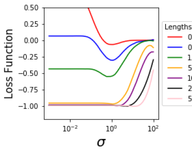
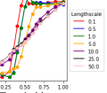
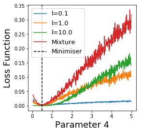
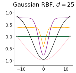
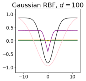
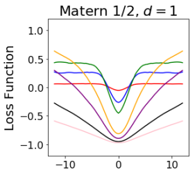
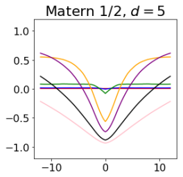
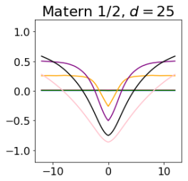
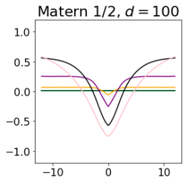
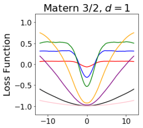
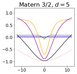
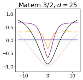
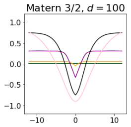
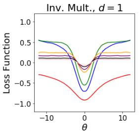
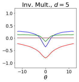
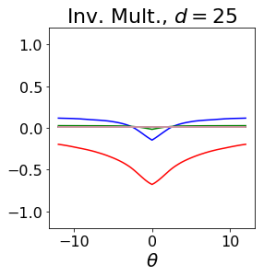
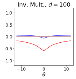
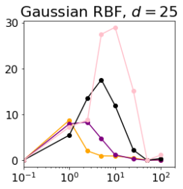
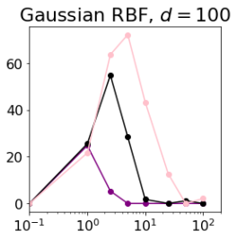
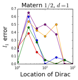
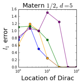
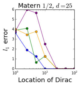
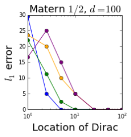
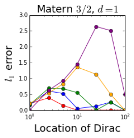
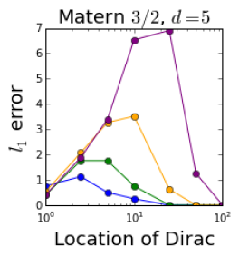
Clearly, the choice of lengthscale can have a significant impact on the efficiency of the estimator, but it can also impact other aspects of the problem. For example, the loss landscape of the MMD, and hence our ability to perform gradient-based optimisation, is severely impacted by the choice of kernel. This is illustrated in Figure 1 (top left) in d=1𝑑1d=1, where choices of lengthscale between 555 and 252525 will be preferable for gradient-based optimisation routines since they avoid large regions where the loss function will have a gradient close to zero. Using a mixture of kernels with a range of lengthscale regimes could help avoid regients of near-zero gradient and hence be generally desirable for the gradient-based optimization. A third aspect of the inference scheme which is impacted by the lengthscale is the robustness. We can quantify the influence of the kernel choice on robustness using the influence function. Similar plots for different classes of kernels can be found in the Appendix in Figures 8, 9 and 10.

Proposition 5 (Influence Function for Gaussian Location Models).

Consider the MMD estimator for the location ΞΈπœƒ\theta of a Gaussian model 𝒩​(ΞΈ,Οƒ2​IdΓ—d)π’©πœƒsuperscript𝜎2subscript𝐼𝑑𝑑\mathcal{N}(\theta,\sigma^{2}I_{d\times d}) based on a Gaussian kernel k​(x,y)=ϕ​(x;y,l2)π‘˜π‘₯𝑦italic-Ο•π‘₯𝑦superscript𝑙2k(x,y)=\phi(x;y,l^{2}). Then the influence function is given by:

IFMMD​(β„™ΞΈ,z)subscriptIFMMDsubscriptβ„™πœƒπ‘§\displaystyle\text{IF}_{\text{MMD}}(\mathbb{P}_{\theta},z) =2​(l2+2​σ2l2+Οƒ2)d2+1​exp⁑(βˆ’β€–zβˆ’ΞΈβ€–222​(l2+Οƒ2))​(zβˆ’ΞΈ).absent2superscriptsuperscript𝑙22superscript𝜎2superscript𝑙2superscript𝜎2𝑑21superscriptsubscriptnormπ‘§πœƒ222superscript𝑙2superscript𝜎2π‘§πœƒ\displaystyle=2\left(\frac{l^{2}+2\sigma^{2}}{l^{2}+\sigma^{2}}\right)^{\frac{d}{2}+1}\exp\left(-\frac{\|z-\theta\|_{2}^{2}}{2(l^{2}+\sigma^{2})}\right)(z-\theta).

Note that the asymptotic variance (6) is minimised by taking l𝑙l arbitrarily large. Despite this, in practice we do not want to choose l𝑙l to be larger than necessary as this will poorly influence the robustness of the estimator. Clearly, for the location model, we see that l𝑙l controls the sensitivity of our estimators. For every finite l𝑙l, we have the following uniform bound for the influence function

supzβˆˆβ„d|IFMMD​(β„™ΞΈβˆ—,z)|subscriptsupremum𝑧superscriptℝ𝑑subscriptIFMMDsubscriptβ„™superscriptπœƒπ‘§\displaystyle\sup_{z\in\mathbb{R}^{d}}\left|\text{IF}_{\operatorname*{\text{MMD}}}(\mathbb{P}_{\theta^{*}},z)\right| =2​eβˆ’1/2​l2+Οƒ2​(l2+2​σ2l2+Οƒ2)d2+1.absent2superscript𝑒12superscript𝑙2superscript𝜎2superscriptsuperscript𝑙22superscript𝜎2superscript𝑙2superscript𝜎2𝑑21\displaystyle=2e^{-1/2}\sqrt{l^{2}+\sigma^{2}}\left(\frac{l^{2}+2\sigma^{2}}{l^{2}+\sigma^{2}}\right)^{\frac{d}{2}+1}.

Taking lβ†’βˆžβ†’π‘™l\rightarrow\infty we have IFMMD​(β„™ΞΈβˆ—,z)β†’(ΞΈβˆ—βˆ’z)β†’subscriptIFMMDsubscriptβ„™superscriptπœƒπ‘§superscriptπœƒπ‘§\text{IF}_{\operatorname*{\text{MMD}}}(\mathbb{P}_{\theta^{*}},z)\rightarrow(\theta^{*}-z), thus losing robustness in the limit. As with asymptotic variance, the sensitivity will depend exponentially on dimension when l𝑙l is small. Contrary to intuition, the uniform influence function minimum will not be attained when l𝑙l approaches zero, but rather at an intermediate point, when l2=d​σ2superscript𝑙2𝑑superscript𝜎2l^{2}=d\sigma^{2}, after which the influence to contamination will increase as lβ†’βˆžβ†’π‘™l\rightarrow\infty. The middle plot in Figure 1 (top) illustrates the effect of kernel bandwidth on robustness. The figure plots the l1subscript𝑙1l_{1} error between the estimated parameter ΞΈ^msubscript^πœƒπ‘š\hat{\theta}_{m} (for n𝑛n) based on a polluted data sample β„šβ€‹(d​x)=(1βˆ’Ο΅)​ϕ​(x;0,1)​d​x+ϡ​δ​zβ„šdπ‘₯1italic-Ο΅italic-Ο•π‘₯01dπ‘₯italic-ϡ𝛿𝑧\mathbb{Q}(\mathrm{d}x)=(1-\epsilon)\phi(x;0,1)\mathrm{d}x+\epsilon\delta z, for some zβˆˆβ„d𝑧superscriptℝ𝑑z\in\mathbb{R}^{d} where Ο΅=0.2italic-Ο΅0.2\epsilon=0.2. While the estimator is qualitatively robust, for higher kernel bandwidths, the estimator will undergo increasingly large excursions from ΞΈβˆ—=0superscriptπœƒ0\theta^{*}=0 as the position of the contaminent point z𝑧z moves to infinity. The second plot demonstrates the behaviour of the estimators as the pollution strength Ο΅italic-Ο΅\epsilon is increased from 00 to 111 and z=(10,…,10)βŠ€π‘§superscript10…10topz=(10,\ldots,10)^{\top}. We observe that for small kernel bandwidths, the estimator undergoes a rapid transition around Ο΅=0.5italic-Ο΅0.5\epsilon=0.5. However, as the lengthscale is increased the estimator becomes increasingly sensitive to distance sample points to the extent that the error grows linearly with respect to Ο΅italic-Ο΅\epsilon. Interestingly, additional experiments presented in Figure 11 of the Appendix indicate that Wasserstein-based estimators may not be robust.
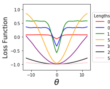
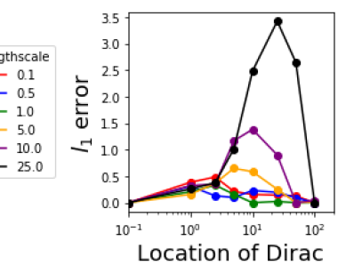
Refer to captionRefer to captionRefer to captionRefer to captionRefer to captionRefer to caption
Refer to caption
Figure 1: Gaussian location and scale models - Performance of the Gaussian RBF kernel (for n,mπ‘›π‘šn,m large). The top plots refer to the Gaussian location model, whilst the bottom plots refer to the Gaussian scale model. Left: Comparison of the loss landscape for various lengthscale values in d=1𝑑1d=1. Center: Robustness problem with varying location xπ‘₯x for the Dirac but threshold fixed to Ο΅=0.2italic-Ο΅0.2\epsilon=0.2 in d=1𝑑1d=1. Right: Robustness problem with varying threshold but fixed location for the Dirac at x=10π‘₯10x=10 in d=1𝑑1d=1.

4.3 Gaussian Scale Model

The second model we consider is a d𝑑d-dimensional isotropic Gaussian distribution 𝒩​(ΞΌ,exp⁑(2​θ)​IdΓ—d)π’©πœ‡2πœƒsubscript𝐼𝑑𝑑\mathcal{N}(\mu,\exp(2\theta)I_{d\times d}) with known location parameter ΞΌβˆˆβ„dπœ‡superscriptℝ𝑑\mu\in\mathbb{R}^{d}. Since the asymptotic variance does not depend on any location parameters of π•Œπ•Œ\mathbb{U}, we will assume without loss of generality that the base measure π•Œπ•Œ\mathbb{U} is a d𝑑d-dimensional Gaussian with mean zero and identity covariance matrix, and that GΞΈ:ℝd→ℝd:subscriptπΊπœƒβ†’superscriptℝ𝑑superscriptℝ𝑑G_{\theta}:\mathbb{R}^{d}\rightarrow\mathbb{R}^{d} is defined by Gθ​(u)=exp⁑(ΞΈ)​usubscriptπΊπœƒπ‘’πœƒπ‘’G_{\theta}(u)=\exp(\theta)u. For simplicity, we assume that we are in the M-closed situation, where the true data distribution β„šβ„š\mathbb{Q} is given by β„™ΞΈβˆ—subscriptβ„™superscriptπœƒ\mathbb{P}_{\theta^{*}} and the kernel is k​(x,y;l)=ϕ​(x;y,l2)π‘˜π‘₯𝑦𝑙italic-Ο•π‘₯𝑦superscript𝑙2k(x,y;l)=\phi(x;y,l^{2}). For this model, the conclusions in terms of efficiency, robustness and loss landscape are similar to those of the Gaussian location model. For example, we can once again compute the asymptotic variance of the CLT:

Proposition 6 (Asymptotic Variance for Gaussian Scale Models).

Consider the minimum MMD estimator for the scale ΞΈπœƒ\theta of a Gaussian distribution 𝒩​(ΞΌ,exp⁑(ΞΈ)​IdΓ—d)π’©πœ‡πœƒsubscript𝐼𝑑𝑑\mathcal{N}(\mu,\exp(\theta)I_{d\times d}) using a Gaussian RBF kernel k​(x,y;l)=ϕ​(x;y,l2)π‘˜π‘₯𝑦𝑙italic-Ο•π‘₯𝑦superscript𝑙2k(x,y;l)=\phi(x;y,l^{2}). The asymptotic variance of the minimum MMD estimator ΞΈ^msubscript^πœƒπ‘š\hat{\theta}_{m} satisfies Cl=gβˆ’1​(ΞΈβˆ—)​Σ​gβˆ’1​(ΞΈβˆ—)superscript𝐢𝑙superscript𝑔1superscriptπœƒΞ£superscript𝑔1superscriptπœƒC^{l}=g^{-1}(\theta^{*})\Sigma g^{-1}(\theta^{*}) where the metric tensor at ΞΈβˆ—superscriptπœƒ\theta^{*} satisfies

g​(ΞΈβˆ—)𝑔superscriptπœƒ\displaystyle g(\theta^{*}) =(2​π)βˆ’d/2​(l2+2​e2β€‹ΞΈβˆ—)βˆ’d/2​d2​K​(d,l,e2β€‹ΞΈβˆ—),absentsuperscript2πœ‹π‘‘2superscriptsuperscript𝑙22superscript𝑒2superscriptπœƒπ‘‘2superscript𝑑2𝐾𝑑𝑙superscript𝑒2superscriptπœƒ\displaystyle=(2\pi)^{-d/2}\left(l^{2}+2e^{2\theta^{*}}\right)^{-d/2}d^{2}K\left(d,l,e^{2\theta^{*}}\right),

for a K​(d,l,s)𝐾𝑑𝑙𝑠K(d,l,s) is bounded with respect to d,l,𝑑𝑙d,l, and s𝑠s and K​(d,0,s)=14​(1+2​dβˆ’1)𝐾𝑑0𝑠1412superscript𝑑1K(d,0,s)=\frac{1}{4}(1+2d^{-1}); and

Ξ£=(2​π)βˆ’d​d2​e4β€‹ΞΈβˆ—β€‹(eΞΈβˆ—+l2)βˆ’2​(C1​(l2+3​e2β€‹ΞΈβˆ—)βˆ’d/2​(l2+e2β€‹ΞΈβˆ—)βˆ’d/2+C2​(l2+2​e2β€‹ΞΈβˆ—)βˆ’d),Ξ£superscript2πœ‹π‘‘superscript𝑑2superscript𝑒4superscriptπœƒsuperscriptsuperscript𝑒superscriptπœƒsuperscript𝑙22subscript𝐢1superscriptsuperscript𝑙23superscript𝑒2superscriptπœƒπ‘‘2superscriptsuperscript𝑙2superscript𝑒2superscriptπœƒπ‘‘2subscript𝐢2superscriptsuperscript𝑙22superscript𝑒2superscriptπœƒπ‘‘\displaystyle\Sigma=(2\pi)^{-d}d^{2}e^{4\theta^{*}}\left(e^{\theta^{*}}+l^{2}\right)^{-2}\left(C_{1}\left(l^{2}+3e^{2\theta^{*}}\right)^{-d/2}\left(l^{2}+e^{2\theta^{*}}\right)^{-d/2}+C_{2}\left(l^{2}+2e^{2\theta^{*}}\right)^{-d}\right),

where C1subscript𝐢1C_{1} and C2subscript𝐢2C_{2} are bounded uniformly with respect to the parameters. Asymptotically, the asymptotic variance behaves as Cl∼(2/3)d/d2similar-tosuperscript𝐢𝑙superscript23𝑑superscript𝑑2C^{l}\sim(2/\sqrt{3})^{d}/d^{2} for lβ‰ͺ1much-less-than𝑙1l\ll 1 and Cl∼l4/d2similar-tosuperscript𝐢𝑙superscript𝑙4superscript𝑑2C^{l}\sim l^{4}/d^{2} for l≫1much-greater-than𝑙1l\gg 1.

This result indicates that the asymptotic variance grows exponentially with dimension as l𝑙l small. In the other extreme, for l𝑙l going to infinity results in an asymptotic variance which is bounded independent of dimension. In fact, the following result characterises the choice of length-scale required for dimension independent efficiency.

Proposition 7 (Critical Scaling for Gaussian Scale Models).

Consider the minimum MMD estimator for the scale ΞΈπœƒ\theta of a Gaussian distribution 𝒩​(ΞΌ,exp⁑(ΞΈ)​IdΓ—d)π’©πœ‡πœƒsubscript𝐼𝑑𝑑\mathcal{N}(\mu,\exp(\theta)I_{d\times d}) with a single Gaussian kernel k​(x,y)=ϕ​(x;y,l2)π‘˜π‘₯𝑦italic-Ο•π‘₯𝑦superscript𝑙2k(x,y)=\phi(x;y,l^{2}) where l=dα𝑙superscript𝑑𝛼l=d^{\alpha}. The asymptotic variance is bounded independently of dimension if and only if Ξ±β‰₯1/4𝛼14\alpha\geq 1/4.

This scaling is the same as for the Gaussian location model, indicating that a more general result on critical scaling for MMD estimators may exists. We reserve this issue for future work. Once again, we notice (Figure 1, bottom left) that the choice of lengthscale has a significant impact on the loss landscape. However, an interesting point is that values of the lengthscale which render the loss landscape easily amenable to gradient-based optimisation are different in the two cases. Numerical experiments clearly indicate that the choice of lengthscale may need to be adapted based on the parameters of interest. The lengthscale has, once again, a significant impact on the robustness of the estimator, as demonstrated in the following result.

Proposition 8 (Influence Function for Gaussian Scale Models).

Consider the minimum MMD estimator for the scale ΞΈπœƒ\theta of a Gaussian model 𝒩​(ΞΌ,exp⁑(ΞΈ)​IdΓ—d)π’©πœ‡πœƒsubscript𝐼𝑑𝑑\mathcal{N}(\mu,\exp(\theta)I_{d\times d}) based on a single Gaussian kernel k​(x,y)=ϕ​(x;y,l2)π‘˜π‘₯𝑦italic-Ο•π‘₯𝑦superscript𝑙2k(x,y)=\phi(x;y,l^{2}). The influence function associated with this estimator is:

IFMMD​(β„™ΞΈ,z)=(l2+2​e2β€‹ΞΈβˆ—l2+e2β€‹ΞΈβˆ—)d2+2​(l2+e2β€‹ΞΈβˆ—βˆ’z2)d​(d+2)​e2β€‹ΞΈβˆ—β€‹exp⁑(βˆ’z22​(l2+e2β€‹ΞΈβˆ—)).subscriptIFMMDsubscriptβ„™πœƒπ‘§superscriptsuperscript𝑙22superscript𝑒2superscriptπœƒsuperscript𝑙2superscript𝑒2superscriptπœƒπ‘‘22superscript𝑙2superscript𝑒2superscriptπœƒsuperscript𝑧2𝑑𝑑2superscript𝑒2superscriptπœƒsuperscript𝑧22superscript𝑙2superscript𝑒2superscriptπœƒ\text{IF}_{\text{MMD}}(\mathbb{P}_{\theta},z)=\left(\frac{l^{2}+2e^{2\theta^{*}}}{l^{2}+e^{2\theta^{*}}}\right)^{\frac{d}{2}+2}\frac{\left(l^{2}+e^{2\theta^{*}}-z^{2}\right)}{d(d+2)e^{2\theta^{*}}}\exp\left(-\frac{z^{2}}{2\left(l^{2}+e^{2\theta^{*}}\right)}\right).

In particular, for every finite l𝑙l we have that

supzβˆˆβ„d|IFMMD​(β„™ΞΈβˆ—,z)|subscriptsupremum𝑧superscriptℝ𝑑subscriptIFMMDsubscriptβ„™superscriptπœƒπ‘§\displaystyle\sup_{z\in\mathbb{R}^{d}}\left|\text{IF}_{\operatorname*{\text{MMD}}}(\mathbb{P}_{{\theta}^{*}},z)\right| =4​eβˆ’3/2​(l2+2​e2β€‹ΞΈβˆ—)d​(d+2)​e2β€‹ΞΈβˆ—β€‹(l2+2​e2β€‹ΞΈβˆ—l2+e2β€‹ΞΈβˆ—)d2+1,absent4superscript𝑒32superscript𝑙22superscript𝑒2superscriptπœƒπ‘‘π‘‘2superscript𝑒2superscriptπœƒsuperscriptsuperscript𝑙22superscript𝑒2superscriptπœƒsuperscript𝑙2superscript𝑒2superscriptπœƒπ‘‘21\displaystyle=\frac{4e^{-3/2}\left(l^{2}+2e^{2\theta^{*}}\right)}{d(d+2)e^{2\theta^{*}}}\left(\frac{l^{2}+2e^{2\theta^{*}}}{l^{2}+e^{2\theta^{*}}}\right)^{\frac{d}{2}+1},

independently of z𝑧z, so that l𝑙l controls the sensitivity of the estimator. Once again, we see exponential dependence on dimension for l𝑙l small, with the minimum uniform influence at an intermediate point, with the dependence increasing as lβ†’βˆžβ†’π‘™l\rightarrow\infty.

4.4 Using Mixtures of Gaussian Kernels

In Li etΒ al. (2015); Ren etΒ al. (2016); Sutherland etΒ al. (2017) it was observed empirically that using mixtures of distributions offers advantageous performance compared to making single choices. In particular, it circumvents issues arising from gradient descent due to vanishing gradients, which can occur if the lengthscale of the kernel chosen to be too small, as can be seen in Figure 1. While multiple kernels offer advantage for gradient descent, we aim to understand where mixture kernels offer any advantages in terms of asymptotic efficiency and robustness. Focusing on the Gaussian location model case, we have the following result.
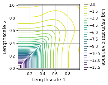
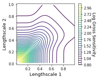
Refer to caption
Refer to caption
Figure 2: Gaussian location model - Efficiency and Robustness for a Mixture of Kernels. Asymptotic variance and gross sensitivity for minimum MMD estimators of the Gaussian location model as a function of l1subscript𝑙1l_{1} and l2subscript𝑙2l_{2} for a mixture of squared exponential kernels: k​(x,y)=exp⁑(βˆ’β€–xβˆ’yβ€–22/2​l12)+exp⁑(βˆ’β€–xβˆ’yβ€–22/2​l22)π‘˜π‘₯𝑦superscriptsubscriptnormπ‘₯𝑦222superscriptsubscript𝑙12superscriptsubscriptnormπ‘₯𝑦222superscriptsubscript𝑙22k(x,y)=\exp(-\|x-y\|_{2}^{2}/2l_{1}^{2})+\exp(-\|x-y\|_{2}^{2}/2l_{2}^{2}).
Proposition 9 (Efficiency and Robustness with Mixture Kernels for Gaussian Location).

Consider the minimum MMD estimator for the location of a Gaussian distribution 𝒩​(ΞΈ,Οƒ2​IdΓ—d)π’©πœƒsuperscript𝜎2subscript𝐼𝑑𝑑\mathcal{N}(\theta,\sigma^{2}I_{d\times d}) using a Gaussian mixture kernel k​(x,y)=βˆ‘s=1SΞ³s​ϕ​(x;y,ls2)π‘˜π‘₯𝑦superscriptsubscript𝑠1𝑆subscript𝛾𝑠italic-Ο•π‘₯𝑦superscriptsubscript𝑙𝑠2k(x,y)=\sum_{s=1}^{S}\gamma_{s}\phi(x;y,l_{s}^{2}). Then the minimimum MMD estimator has asymptotic variance given by

Οƒ2β€‹βˆ‘s=1Sβˆ‘sβ€²=1SΞ³s​γs′​((ls2+Οƒ2)​(lsβ€²2+Οƒ2)+Οƒ2​(2​σ2+ls2+lsβ€²2))βˆ’d2βˆ’1(βˆ‘s=1SΞ³s​(ls2+2​σ2)βˆ’d2βˆ’1)2​IdΓ—d.superscript𝜎2superscriptsubscript𝑠1𝑆superscriptsubscriptsuperscript𝑠′1𝑆subscript𝛾𝑠subscript𝛾superscript𝑠′superscriptsuperscriptsubscript𝑙𝑠2superscript𝜎2superscriptsubscript𝑙superscript𝑠′2superscript𝜎2superscript𝜎22superscript𝜎2superscriptsubscript𝑙𝑠2superscriptsubscript𝑙superscript𝑠′2𝑑21superscriptsuperscriptsubscript𝑠1𝑆subscript𝛾𝑠superscriptsuperscriptsubscript𝑙𝑠22superscript𝜎2𝑑212subscript𝐼𝑑𝑑\sigma^{2}\frac{\sum_{s=1}^{S}\sum_{s^{\prime}=1}^{S}\gamma_{s}\gamma_{s^{\prime}}\left((l_{s}^{2}+\sigma^{2})(l_{s^{\prime}}^{2}+\sigma^{2})+\sigma^{2}(2\sigma^{2}+l_{s}^{2}+l_{s^{\prime}}^{2})\right)^{-\frac{d}{2}-1}}{\left(\sum_{s=1}^{S}\gamma_{s}(l_{s}^{2}+2\sigma^{2})^{-\frac{d}{2}-1}\right)^{2}}I_{d\times d}. (7)

Furthermore, the influence function is given by:

IFMMD​(z,β„™ΞΈ)subscriptIFMMD𝑧subscriptβ„™πœƒ\displaystyle\text{IF}_{\text{MMD}}(z,\mathbb{P}_{\theta}) =2β€‹βˆ‘s=1SΞ³s​(ls2+Οƒ2)βˆ’d2βˆ’1​exp⁑(βˆ’β€–zβˆ’ΞΈβ€–222​(ls2+Οƒ2))​(zβˆ’ΞΈ)βˆ‘s=1SΞ³s​(ls2+2​σ2)βˆ’d2βˆ’1.absent2superscriptsubscript𝑠1𝑆subscript𝛾𝑠superscriptsuperscriptsubscript𝑙𝑠2superscript𝜎2𝑑21superscriptsubscriptnormπ‘§πœƒ222superscriptsubscript𝑙𝑠2superscript𝜎2π‘§πœƒsuperscriptsubscript𝑠1𝑆subscript𝛾𝑠superscriptsuperscriptsubscript𝑙𝑠22superscript𝜎2𝑑21\displaystyle=\frac{2\sum_{s=1}^{S}\gamma_{s}(l_{s}^{2}+\sigma^{2})^{-\frac{d}{2}-1}\exp\left(-\frac{\|z-\theta\|_{2}^{2}}{2(l_{s}^{2}+\sigma^{2})}\right)(z-\theta)}{\sum_{s=1}^{S}\gamma_{s}(l_{s}^{2}+2\sigma^{2})^{-\frac{d}{2}-1}}.

In Figure 2 we plot the log asymptotic variance and log gross sensitivity for the Gaussian location model based on a mixture kernel composed of two Gaussian kernels with lengthscales l1subscript𝑙1l_{1} and l2subscript𝑙2l_{2}. What is interesting to note that there are choices of (l1,l2)subscript𝑙1subscript𝑙2(l_{1},l_{2}) which give rise to higher efficiency and robustness than their individual counterparts. Indeed, for example, choosing l1=0.8subscript𝑙10.8l_{1}=0.8 then the asymptotic variance will be minimised when l2β‰ˆ0.6subscript𝑙20.6l_{2}\approx 0.6, although this choice will reduce bias-robustness. This figure appears to support the claim that mixture kernels can also provide increased performance beyond assisting gradient descent, and merits further investigation.

5 Numerical Experiments

In this final section, we examine the impact of the choice of kernel on several applications. In particular, we highlight the importance of working with estimators which are robust to model misspecification. We start with two applications which are popular test-beds for inference for intractable generative models: the g-and-k distribution and a stochastic volatility model. We then move on to a problem of parameter inference for systems of stochastic differential equations, where we consider a parameter-prey model and a multiscale model. These examples allow us to demonstrate the advantage of our natural gradient descent algorithm, and the favourable robustness properties of the estimators.

5.1 G-and-k distribution

A common synthetic model in the literature on generative models is the g-and-k distribution (Bernton etΒ al., 2019; Prangle, 2017). For this model, we only have access to the quantile function GΞΈ:[0,1]→ℝ:subscriptπΊπœƒβ†’01ℝG_{\theta}:[0,1]\rightarrow\mathbb{R} (also called inverse cumulative distribution function) given by:

Gθ​(u)subscriptπΊπœƒπ‘’\displaystyle G_{\theta}(u) :=a+b​(1+0.8​(1βˆ’exp(βˆ’cΞ¦βˆ’1(u;0,1))(1+exp(βˆ’cΞ¦βˆ’1(u;0,1)))​(1+(Ξ¦βˆ’1​(u;0,1))2)kβ€‹Ξ¦βˆ’1​(u;0,1)\displaystyle:=a+b\left(1+0.8\frac{\big{(}1-\exp(-c\Phi^{-1}(u;0,1)\big{)}}{\big{(}1+\exp(-c\Phi^{-1}(u;0,1)\big{)}}\right)\big{(}1+(\Phi^{-1}(u;0,1))^{2}\big{)}^{k}\Phi^{-1}(u;0,1)

where Ξ¦βˆ’1​(u;0,1)superscriptΞ¦1𝑒01\Phi^{-1}(u;0,1) refers to the u𝑒u’th quantile of the standard normal distribution. The parameter of interest is ΞΈ=(ΞΈ1,ΞΈ2,ΞΈ3,ΞΈ4)πœƒsubscriptπœƒ1subscriptπœƒ2subscriptπœƒ3subscriptπœƒ4\theta=(\theta_{1},\theta_{2},\theta_{3},\theta_{4}) where ΞΈ1=asubscriptπœƒ1π‘Ž\theta_{1}=a controls location, ΞΈ2=bsubscriptπœƒ2𝑏\theta_{2}=b controls scale, ΞΈ3=csubscriptπœƒ3𝑐\theta_{3}=c controls skewness and ΞΈ4=exp⁑(k)subscriptπœƒ4π‘˜\theta_{4}=\exp(k) controls kurtosis. Although this is a model defined on a one-dimensional space, the four parameters allow for a very flexible family of distributions. A rescaling of the last parameter is used to avoid instabilities. Since the quantile function is available, we can easily simulate from this model using inverse transform sampling.

We study the behaviour of the MMD estimators for this model in Figure 3. For the left and center plots, we used both stochastic gradient descent and stochastic gradient descent with preconditioner to obtain an estimate of ΞΈ^msubscript^πœƒπ‘š\hat{\theta}_{m}. We used a constant step-size for both algorithms (tuned for good performance) and ran each algorithm for 500500500 iterations. The data is of size m=30000π‘š30000m=30000 but we used minibatches of size 200200200, the simulated data was of size n=200𝑛200n=200, the kernel was Gaussian RBF with lengthscale l=2𝑙2l=2 and ΞΈβˆ—=(3,1,1,βˆ’log⁑(2))superscriptπœƒ3112\theta^{*}=(3,1,1,-\log(2)). The large number of data points is used to guarantee that the minimiser can be recovered. We notice that both the stochastic gradient descent and stochastic natural gradient descent are able to recover ΞΈ1βˆ—superscriptsubscriptπœƒ1\theta_{1}^{*} and ΞΈ2βˆ—superscriptsubscriptπœƒ2\theta_{2}^{*} for a variety of initial conditions in the neighbourhood of the minimiser. On the other hand, as observed in the center plot, the stochastic gradient descent algorithm is very slow for ΞΈ3βˆ—superscriptsubscriptπœƒ3\theta_{3}^{*} and ΞΈ4βˆ—superscriptsubscriptπœƒ4\theta_{4}^{*}, whereas the natural stochastic gradient descent algorithm is able to recover both of these parameters in a small number of steps. This clearly highlights the advantage of the rescaling of the parameter space provided by the preconditionner based on the geometry induced by the information metric.
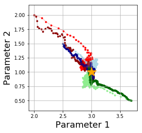
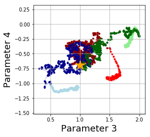
Refer to caption
Refer to caption
Refer to caption
Figure 3: Inference for the parameters of the g-and-k distribution using a maximum mean discrepancy estimator. Left & Center: Several runs of a stochastic gradient descent (light blue, light red and light green) and a stochastic natural gradient descent (dark blue, dark red and dark green) algorithm on the MMD loss function with Gaussian RBF kernel with lengthscale l=2𝑙2l=2. The black dot corresponds to the minimiser. Right: Estimate of the MMD loss function around the minimum as a function of ΞΈ4subscriptπœƒ4\theta_{4} for a Gaussian RBF kernel with varying choices of lengthscales and a mixture of all the Gaussian kernels.

We also plot the MMD loss function as a function of ΞΈ4subscriptπœƒ4\theta_{4} in the neighborhood of ΞΈβˆ—superscriptπœƒ\theta^{*}. The estimator is sensitive to the choice of lengthscale: in the case where we use a Gaussian RBF kernel, a lengthscale smaller of equal to l=0.1𝑙0.1l=0.1 or greater or equal to l=10𝑙10l=10 led to a loss function which is flat on a wide range of the space. In those cases, it will be difficult to obtain an accurate estimate of the parameter due to the noise in our estimates of the gradient. On the other hand, a lengthscale of l=1𝑙1l=1 allows us to provide more accurate results. Furthermore, the use of a mixture of all of these kernels also allows us to obtain accurate results without having to manually tune the choice of lenghtscale.

5.2 Stochastic Volatility Model with Gaussian and Cauchy Noise

Our second model is a stochastic volatility model (Kim etΒ al., 1998), popular in the econometrics literature as a model of the returns on assets over time. The model can be simulated from by sampling the first hidden variable h1βˆΌπ’©β€‹(0,Οƒ2/(1βˆ’Ο•2))similar-tosubscriptβ„Ž1𝒩0superscript𝜎21superscriptitalic-Ο•2h_{1}\sim\mathcal{N}(0,\sigma^{2}/(1-\phi^{2})) representing the initial volatility, then following the following set of equations:

htsubscriptβ„Žπ‘‘\displaystyle h_{t} =ϕ​htβˆ’1+Ξ·t,Ξ·tβˆΌπ’©β€‹(0,Οƒ2),formulae-sequenceabsentitalic-Ο•subscriptβ„Žπ‘‘1subscriptπœ‚π‘‘similar-tosubscriptπœ‚π‘‘π’©0superscript𝜎2\displaystyle=\phi h_{t-1}+\eta_{t},\qquad\eta_{t}\;\sim\;\mathcal{N}(0,\sigma^{2}),
ytsubscript𝑦𝑑\displaystyle y_{t} =Ο΅t​κ​exp⁑(0.5​ht),Ο΅tβˆΌπ’©β€‹(0,1).formulae-sequenceabsentsubscriptitalic-Ο΅π‘‘πœ…0.5subscriptβ„Žπ‘‘similar-tosubscriptitalic-ϡ𝑑𝒩01\displaystyle=\epsilon_{t}\kappa\exp(0.5h_{t}),\qquad\epsilon_{t}\;\sim\;\mathcal{N}(0,1).

where ytsubscript𝑦𝑑y_{t} is the mean corrected return on holding an asset at time t𝑑t, and htsubscriptβ„Žπ‘‘h_{t} the log-volatility at time t𝑑t. The {yt}t=1Tsuperscriptsubscriptsubscript𝑦𝑑𝑑1𝑇\{y_{t}\}_{t=1}^{T} are observed data and {ht}t=1Tsuperscriptsubscriptsubscriptβ„Žπ‘‘π‘‘1𝑇\{h_{t}\}_{t=1}^{T} are unobserved latent variables. This is therefore a generative model with parameters (Ο•,ΞΊ,Οƒ)italic-Ο•πœ…πœŽ(\phi,\kappa,\sigma), which we reparameterised with ΞΈ1=log⁑((1+Ο•)/(1βˆ’Ο•)),ΞΈ2=log⁑κ,ΞΈ3=log⁑(Οƒ2)formulae-sequencesubscriptπœƒ11italic-Ο•1italic-Ο•formulae-sequencesubscriptπœƒ2πœ…subscriptπœƒ3superscript𝜎2\theta_{1}=\log((1+\phi)/(1-\phi)),\theta_{2}=\log\kappa,\theta_{3}=\log(\sigma^{2}) to avoid numerical issues so that we want to recover ΞΈ=(ΞΈ1,ΞΈ2,ΞΈ3)πœƒsubscriptπœƒ1subscriptπœƒ2subscriptπœƒ3\theta=(\theta_{1},\theta_{2},\theta_{3}). The data dimension is d=T𝑑𝑇d=T and the parametric dimension is p=3𝑝3p=3. The likelihood of these models is usually not available in closed form due to the presence of latent variables and hence given by p​(y1,…,yT|ΞΈ)=∫p​(y1,…,yT|h1,…,hT,ΞΈ)​p​(h1,…,hT|ΞΈ)​dh1​…​dhT𝑝subscript𝑦1…conditionalsubscriptπ‘¦π‘‡πœƒπ‘subscript𝑦1…conditionalsubscript𝑦𝑇subscriptβ„Ž1…subscriptβ„Žπ‘‡πœƒπ‘subscriptβ„Ž1…conditionalsubscriptβ„Žπ‘‡πœƒdifferential-dsubscriptβ„Ž1…differential-dsubscriptβ„Žπ‘‡p(y_{1},\ldots,y_{T}|\theta)=\int p(y_{1},\ldots,y_{T}|h_{1},\ldots,h_{T},\theta)p(h_{1},\ldots,h_{T}|\theta)\mathrm{d}h_{1}\ldots\mathrm{d}h_{T} which is a high-dimensional intractable integral. Alternative approaches based on quasi-likelihood estimation or expectation-maximisation can be considered, but the approximation obtained may be unreliable. Furthermore, it may be preferable to make use of minimum MMD estimators since these will allow for robust inference, which is not the case for alternative approaches.

In our experiments, we choose T=30𝑇30T=30 and considered inference with minimum MMD estimators with Gaussian kernels. Initially, we considered the M-closed case and generated m=20000π‘š20000m=20000 data points for ΞΈβˆ—=(0.98,0.65,0.15)superscriptπœƒ0.980.650.15\theta^{*}=(0.98,0.65,0.15), which we then tried to infer by minimising the MMD loss function with a wide range of kernels. For the experimental results, we used stochastic gradient descent and stochastic natural gradient descent with minibatches of size 200020002000, and used n=45𝑛45n=45. Results in Figure 4 (top) demonstrate that our natural gradient algorithm is able to recover the parameters in around five thousand iterations whereas the gradient descent algorithm isn’t close to convergence after 300003000030000 steps. Note that even though the dimension d=30𝑑30d=30, the parameter space has dimension p=3𝑝3p=3 so that the additional computational cost of the preconditioner is negligeable for this problem (and completely dwarfed by the cost of the generator).
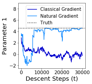
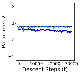
Refer to caption
Refer to caption
Refer to caption
Refer to caption
Refer to caption
Refer to caption
Refer to caption
Refer to caption
Refer to caption
Figure 4: Inference for stochastic volatility models. Top: Well-specified case - Gradient descent and natural gradient descent on the MMD loss function with a mixture of Gaussian RBF kernels with lengthscales 1,5,10,20,40151020401,5,10,20,40. Bottom: Misspecified case - Gradient descent on the MMD loss function with a variety of kernels including a Gaussian RBF kernel with lengthscales 111, 555, 101010, 202020, as well as a mixture of all these kernels and a Gaussian RBF kernel with lengthscale l=40𝑙40l=40.

We then considered the M-open case, and introduced misspecification by simulating the Ο΅tsubscriptitalic-ϡ𝑑\epsilon_{t} values using IID realisations of a Cauchy distribution with location parameter 00 and scale parameter 2/Ο€2πœ‹\sqrt{2/\pi}. This distribution has the same median as the Gaussian distribution, and their probability density functions match at that point, but the Cauchy has much fatter tails. The results of these experiments are available in Figure 4, and in each case we repeated the experiments with 444 different stepsize choices and plot the best result. In the well-specified case, we notice that the natural gradient descent algorithm is able to take advantage of the local geometry of the problem and converges to ΞΈβˆ—superscriptπœƒ\theta^{*} in a small number of iterations. Further experiments with a larger range of kernels is available in Appendix D.3, but the mixture kernel tended to work best.

In the misspecified case, we notice (as expected) that while none of the minimum MMD estimators is able to recover the true value of ΞΈβˆ—superscriptπœƒ\theta^{*}, but that the inferred results remain stable, i.e. close to the truth. The choice of kernel has a clear impact on the output. For Gaussian RBF kernels with lengthscales l=1𝑙1l=1 or l=5𝑙5l=5, the loss function is too flat for gradient descent and we are not able to move much from the initial parameter. For larger values of the lengthscale (e.g. l=10,20,40𝑙102040l=10,20,40) and for the mixture kernel, we are able to use gradient-based optimisation but that it demonstrates increased sensitivity to model mispecification. We note that the single Gaussian RBF kernels with large lengthscale are able to learn ΞΈ1βˆ—superscriptsubscriptπœƒ1\theta_{1}^{*} well in the sense that there is negligeable bias as compared to ΞΈ2βˆ—superscriptsubscriptπœƒ2\theta_{2}^{*} and ΞΈ3βˆ—superscriptsubscriptπœƒ3\theta_{3}^{*}. This is likely due to the improvement in bias robustness expected for kernels with large lengthscale.

5.3 Inference for Systems of Stochastic Differential Equations

For our third set of experiments, we use minimum MMD estimation to infer the initial condition and parameters for coupled systems of stochastic differential equations (SDEs). In general, will will consider a d𝑑d-dimensional ItΓ΄ stochastic differential equation of the form

d​Xt=b​(Xt;ΞΈ1)​d​t+σ​(Xt;ΞΈ1)​d​Wt,𝑑subscript𝑋𝑑𝑏subscript𝑋𝑑subscriptπœƒ1π‘‘π‘‘πœŽsubscript𝑋𝑑subscriptπœƒ1𝑑subscriptπ‘Šπ‘‘\displaystyle dX_{t}=b(X_{t};\theta_{1})\,dt+\sigma(X_{t};\theta_{1})\,dW_{t}, (8)

where b:ℝdΓ—Ξ˜β†’β„d:𝑏→superscriptβ„π‘‘Ξ˜superscriptℝ𝑑b:\mathbb{R}^{d}\times\Theta\rightarrow\mathbb{R}^{d}, Οƒ:ℝdΓ—Ξ˜β†’β„dΓ—k:πœŽβ†’superscriptβ„π‘‘Ξ˜superscriptβ„π‘‘π‘˜\sigma:\mathbb{R}^{d}\times\Theta\rightarrow\mathbb{R}^{d\times k}, Wtsubscriptπ‘Šπ‘‘W_{t} is a kπ‘˜k dimensional standard Brownian motion and with initial value X0=ΞΈ2subscript𝑋0subscriptπœƒ2X_{0}=\theta_{2} and where (ΞΈ1,ΞΈ2)∈Θsubscriptπœƒ1subscriptπœƒ2Θ(\theta_{1},\theta_{2})\in\Theta is a vector of unknown parameters to be determined. We assume that for each ΞΈπœƒ\theta there is a unique solution to (8) which depends continuously on the initial condition.

For any fixed ΞΈπœƒ\theta, provided we can simulate X​(t)𝑋𝑑X(t), at points 0=t0<t1<…<tK=T0subscript𝑑0subscript𝑑1…subscript𝑑𝐾𝑇0=t_{0}<t_{1}<\ldots<t_{K}=T, then we can consider the generative model defined by β„™ΞΈ=GΞΈ#β€‹π•Œsubscriptβ„™πœƒsuperscriptsubscriptπΊπœƒ#π•Œ\mathbb{P}_{\theta}=G_{\theta}^{\#}\mathbb{U}, where π•Œπ•Œ\mathbb{U} is the Wiener path measure for a kπ‘˜k dimensional standard Wiener process on C​[0,T]𝐢0𝑇C[0,T] and GΞΈ=Oθ∘IΞΈsubscriptπΊπœƒsubscriptπ‘‚πœƒsubscriptπΌπœƒG_{\theta}=O_{\theta}\circ I_{\theta}, where IΞΈ:C​[0,T]β†’C​[0,T]:subscriptπΌπœƒβ†’πΆ0𝑇𝐢0𝑇I_{\theta}:C[0,T]\rightarrow C[0,T] is the ItΓ΄ map, transforming the Wiener process to the solution X​(β‹…)𝑋⋅X(\cdot) of the SDE. Here, OΞΈsubscriptπ‘‚πœƒO_{\theta} is an observation operator, for example mapping w∈C​[0,T]𝑀𝐢0𝑇w\in C[0,T] to (w​(t1),…,w​(tK))𝑀subscript𝑑1…𝑀subscript𝑑𝐾(w(t_{1}),\ldots,w(t_{K})) or any other smooth functional of the path which depends smoothly on ΞΈπœƒ\theta. Note that it is trivial to incorporate observational noise and volatility parameters into the observation operator.

To perform MMD gradient descent for this model we must calculate the gradient of the forward map with respect to the parameters ΞΈπœƒ\theta. Pathwise derivatives of the solution of (8) with respect to initial conditions and coefficient parameters are well established (Kunita, 1997; Gobet and Munos, 2005; Friedman, 2012) and are detailed in the following result; see also Tzen and Raginsky (2019) for a similar result arising in a similar context.

Proposition 10.

(Kunita, 1997, Theorem 2.3.1) Suppose that the drift b​(x;ΞΈ1)𝑏π‘₯subscriptπœƒ1b(x;\theta_{1}) and diffusion tensor σ​(x;ΞΈ1)𝜎π‘₯subscriptπœƒ1\sigma(x;\theta_{1}) are Lipschitz with Lipschitz derivatives with respect to xπ‘₯x and ΞΈ1subscriptπœƒ1\theta_{1}. Then the pathwise derivative of Xtsubscript𝑋𝑑X_{t} with respect to the parameters ΞΈ1subscriptπœƒ1\theta_{1} is given by the solution of the Ito process,

d​(βˆ‡ΞΈ1Xt)=𝑑subscriptβˆ‡subscriptπœƒ1subscript𝑋𝑑absent\displaystyle d\left(\nabla_{\theta_{1}}X_{t}\right)= (βˆ‡xb​(Xt;ΞΈ1)β€‹βˆ‡ΞΈ1Xt+βˆ‡ΞΈ1b​(Xt;ΞΈ1))​d​t+(βˆ‡xσ​(Xt;ΞΈ)β€‹βˆ‡ΞΈ1Xt+βˆ‡ΞΈ1σ​(Xt;ΞΈ1))​d​Wtsubscriptβˆ‡π‘₯𝑏subscript𝑋𝑑subscriptπœƒ1subscriptβˆ‡subscriptπœƒ1subscript𝑋𝑑subscriptβˆ‡subscriptπœƒ1𝑏subscript𝑋𝑑subscriptπœƒ1𝑑𝑑subscriptβˆ‡π‘₯𝜎subscriptπ‘‹π‘‘πœƒsubscriptβˆ‡subscriptπœƒ1subscript𝑋𝑑subscriptβˆ‡subscriptπœƒ1𝜎subscript𝑋𝑑subscriptπœƒ1𝑑subscriptπ‘Šπ‘‘\displaystyle\left(\nabla_{x}b(X_{t};\theta_{1})\nabla_{\theta_{1}}X_{t}+\nabla_{\theta_{1}}b(X_{t};\theta_{1})\right)\,dt+\left(\nabla_{x}\sigma(X_{t};\theta)\nabla_{\theta_{1}}X_{t}+\nabla_{\theta_{1}}\sigma(X_{t};\theta_{1})\right)\,dW_{t}

with initial condition βˆ‡ΞΈ1X0=𝟎subscriptβˆ‡subscriptπœƒ1subscript𝑋00\nabla_{\theta_{1}}X_{0}=\mathbf{0} and the derivative of Xtsubscript𝑋𝑑X_{t} with respect to ΞΈ2subscriptπœƒ2\theta_{2} is given by

d​(βˆ‡ΞΈ2Xt)=𝑑subscriptβˆ‡subscriptπœƒ2subscript𝑋𝑑absent\displaystyle d\left(\nabla_{\theta_{2}}X_{t}\right)= (βˆ‡xb​(Xt;ΞΈ1)β€‹βˆ‡ΞΈ2Xt)​d​t+(βˆ‡xσ​(Xt;ΞΈ)β€‹βˆ‡ΞΈ2Xt)​d​Wt,subscriptβˆ‡π‘₯𝑏subscript𝑋𝑑subscriptπœƒ1subscriptβˆ‡subscriptπœƒ2subscript𝑋𝑑𝑑𝑑subscriptβˆ‡π‘₯𝜎subscriptπ‘‹π‘‘πœƒsubscriptβˆ‡subscriptπœƒ2subscript𝑋𝑑𝑑subscriptπ‘Šπ‘‘\displaystyle\left(\nabla_{x}b(X_{t};\theta_{1})\nabla_{\theta_{2}}X_{t}\right)\,dt+\left(\nabla_{x}\sigma(X_{t};\theta)\nabla_{\theta_{2}}X_{t}\right)\,dW_{t},

where βˆ‡ΞΈ2X0=Isubscriptβˆ‡subscriptπœƒ2subscript𝑋0𝐼\nabla_{\theta_{2}}X_{0}=I. In particular, given a differentiable function F𝐹F of Xt0,…,XtKsubscript𝑋subscript𝑑0…subscript𝑋subscript𝑑𝐾X_{t_{0}},\ldots,X_{t_{K}},

βˆ‡ΞΈi𝔼​[F​(Xt0,…,XtK)]subscriptβˆ‡subscriptπœƒπ‘–π”Όdelimited-[]𝐹subscript𝑋subscript𝑑0…subscript𝑋subscript𝑑𝐾\displaystyle\nabla_{\theta_{i}}\mathbb{E}\left[F(X_{t_{0}},\ldots,X_{t_{K}})\right] =𝔼​[βˆ‘k=1Kβˆ‡xkF​(Xt0,…,XtK)β€‹βˆ‡ΞΈiXtk],Β for ​i=1,2.formulae-sequenceabsent𝔼delimited-[]superscriptsubscriptπ‘˜1𝐾subscriptβˆ‡subscriptπ‘₯π‘˜πΉsubscript𝑋subscript𝑑0…subscript𝑋subscript𝑑𝐾subscriptβˆ‡subscriptπœƒπ‘–subscript𝑋subscriptπ‘‘π‘˜Β for 𝑖12\displaystyle=\mathbb{E}\left[\sum_{k=1}^{K}\nabla_{x_{k}}F(X_{t_{0}},\ldots,X_{t_{K}})\nabla_{\theta_{i}}X_{t_{k}}\right],\quad\text{ for }i=1,2.

Before moving on to the experiments, we note that Abbati etΒ al. (2019) proposed an alternative method, performing Gaussian process-based gradient matching for ODEs and SDEs with additive noise, by using MMD to fit a GP process inferred from the data to the SDE. However, the approach we propose permits parametric estimation for more general SDEs and noise models.

5.3.1 Noisy Lotka-Volterra Model with Unknown Initial Conditions

As an example, we consider the stochastic Lotka-Volterra model (Volterra, 1926), which consists of a pair of nonlinear differential equations describing the evolution of two species through time:

d​(X1,tX2,t)dsubscript𝑋1𝑑subscript𝑋2𝑑\displaystyle\mathrm{d}\left(\begin{array}[]{c}X_{1,t}\\ X_{2,t}\end{array}\right) =[(10)​θ11​X1,t+(βˆ’11)​θ12​X1,t​X2,t+(0βˆ’1)​θ13​X2,t]​d​tabsentdelimited-[]10subscriptπœƒ11subscript𝑋1𝑑11subscriptπœƒ12subscript𝑋1𝑑subscript𝑋2𝑑01subscriptπœƒ13subscript𝑋2𝑑d𝑑\displaystyle=\left[\left(\begin{array}[]{c}1\\ 0\end{array}\right)\theta_{11}X_{1,t}+\left(\begin{array}[]{c}-1\\ 1\end{array}\right)\theta_{12}X_{1,t}X_{2,t}+\left(\begin{array}[]{c}0\\ -1\end{array}\right)\theta_{13}X_{2,t}\right]\mathrm{d}t
+(10)​θ11​X1,t​d​Wt(1)+(βˆ’11)​θ12​X1,t​X2,t​d​Wt(2)+(0βˆ’1)​θ13​X2,t​d​Wt(3),10subscriptπœƒ11subscript𝑋1𝑑dsuperscriptsubscriptπ‘Šπ‘‘111subscriptπœƒ12subscript𝑋1𝑑subscript𝑋2𝑑dsuperscriptsubscriptπ‘Šπ‘‘201subscriptπœƒ13subscript𝑋2𝑑dsuperscriptsubscriptπ‘Šπ‘‘3\displaystyle+\left(\begin{array}[]{c}1\\ 0\end{array}\right)\sqrt{\theta_{11}X_{1,t}}\mathrm{d}W_{t}^{(1)}+\left(\begin{array}[]{c}-1\\ 1\end{array}\right)\sqrt{\theta_{12}X_{1,t}X_{2,t}}\mathrm{d}W_{t}^{(2)}+\left(\begin{array}[]{c}0\\ -1\end{array}\right)\sqrt{\theta_{13}X_{2,t}}\mathrm{d}W_{t}^{(3)},

where the initial conditions ΞΈ2=(X1,0,X2,0)subscriptπœƒ2subscript𝑋10subscript𝑋20\theta_{2}=(X_{1,0},X_{2,0}) are unknown, but the parameters ΞΈ1=(ΞΈ11,ΞΈ12,ΞΈ13)subscriptπœƒ1subscriptπœƒ11subscriptπœƒ12subscriptπœƒ13\theta_{1}=(\theta_{11},\theta_{12},\theta_{13}) governing the dynamics are known. While exact sampling methods for diffusions exist, see Beskos and Roberts (2005), for simplicity we shall employ an inexact Euler-Maruyama discretisation, choosing the step size sufficiently small to ensure stability of the discretisation. We choose the β€œtrue” initial condition to be deterministic with value ΞΈ2βˆ—=(X1,0,X2,0)superscriptsubscriptπœƒ2subscript𝑋10subscript𝑋20\theta_{2}^{*}=(X_{1,0},X_{2,0}). We fix a-priori the time horizon to T=1𝑇1T=1 and the parameters governing the equation to ΞΈ1=(ΞΈ11,ΞΈ12,ΞΈ13)=(5,0.025,6)subscriptπœƒ1subscriptπœƒ11subscriptπœƒ12subscriptπœƒ1350.0256\theta_{1}=(\theta_{11},\theta_{12},\theta_{13})=(5,0.025,6). In this case, p=2𝑝2p=2, d=2𝑑2d=2 and n𝑛n tends to be small (in the tens or hundreds). We consider the case where n=50𝑛50n=50.

Refer to caption
Refer to caption
Figure 5: Inference for the initial conditions of a Lotka-Volterra model with noisy dynamics. Left: n=100𝑛100n=100 realisations from the coupled stochastic differential equations for several initial conditions. Right: n=100𝑛100n=100 realisations used for inference, including 909090 realisations from the correct model and 101010 which are corrupted.

Typical realisations for the system of coupled stochastic differential equations can be found in Figure 5 (left) for several values of the initial conditions. As we would expect, the closer the initial conditions, the closer the realisations of stochastic differential equations will be. This clearly motivates the use of minimum MMD estimators. We are particularly interested interested in the behaviour of the estimators as a proportion of the data is corrupted. In particular, we will consider the problem of inferring initial conditions ΞΈ2βˆ—=(100,120)subscriptsuperscriptπœƒ2100120\theta^{*}_{2}=(100,120) given realisations from this model which are corrupted by realisations from the model initialised at ΞΈ2†=(50,50)subscriptsuperscriptπœƒβ€ 25050\theta^{\dagger}_{2}=(50,50). Realisations are provided in Figure 5 (right) for the case with 10%percent1010\% misspecification.

We expect this type of misspecification to lead to severe issues for non-robust inference algorithms, but the bias robustness of minimum MMD estimators allows us to provide reasonable estimates of the parameter. This can be seen in Figure 6 (left) where we plot estimates provided by MMD estimators for ΞΈ22subscriptπœƒ22\theta_{22} as a function of natural gradient steps for various proportion levels of corruption. This is compared to the Sinkhorn algorithm of Genevay etΒ al. (2018). As can be seen, the MMD estimator can recover the truth for a large proportion of corrupted samples whereas Wasserstein-based estimators are very sensitive to corrupted data.
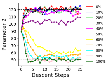
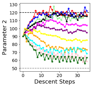
Refer to caption
Refer to caption
Figure 6: Inference for the initial conditions of a Lotka-Volterra model with corrupted observations based on m=100π‘š100m=100 realisations and n=50𝑛50n=50 simulated data. Each color correspond to a different percentage of corrupted observations. Left: Stochastic gradient descent steps for minimum Sinkhorn estimator with l2subscript𝑙2l_{2} cost and Ο΅=1italic-Ο΅1\epsilon=1 regularisation. Right: Stochastic gradient descent steps for minimum MMD estimator with Gaussian RBF kernel and lengthscale l=30𝑙30l=30.

5.3.2 Parametric Inference for a System of SDEs with Multiple Scales

We consider a second example where we observe realisations of the following two-dimensional multiscale system

d​Xtϡ𝑑subscriptsuperscript𝑋italic-ϡ𝑑\displaystyle dX^{\epsilon}_{t} =(ΞΈ12ϡ​YtΟ΅+ΞΈ11​XtΟ΅)​d​t,d​YtΟ΅=βˆ’1Ο΅2​Ytϡ​d​t+2ϡ​d​Wt,formulae-sequenceabsentsubscriptπœƒ12italic-Ο΅subscriptsuperscriptπ‘Œitalic-ϡ𝑑subscriptπœƒ11subscriptsuperscript𝑋italic-ϡ𝑑𝑑𝑑𝑑subscriptsuperscriptπ‘Œitalic-ϡ𝑑1superscriptitalic-Ο΅2subscriptsuperscriptπ‘Œitalic-ϡ𝑑𝑑𝑑2italic-ϡ𝑑subscriptπ‘Šπ‘‘\displaystyle=\left(\frac{\sqrt{\theta_{12}}}{\epsilon}Y^{\epsilon}_{t}+\theta_{11}X^{\epsilon}_{t}\right)\,dt,\qquad dY^{\epsilon}_{t}=-\frac{1}{\epsilon^{2}}Y^{\epsilon}_{t}\,dt+\frac{\sqrt{2}}{\epsilon}dW_{t}, (9)

where Wtsubscriptπ‘Šπ‘‘W_{t} is a standard Brownian motion, 0<Ο΅β‰ͺ10italic-Ο΅much-less-than10<\epsilon\ll 1 is a small length-scale parameter, ΞΈ1=(ΞΈ11,ΞΈ12)subscriptπœƒ1subscriptπœƒ11subscriptπœƒ12\theta_{1}=(\theta_{11},\theta_{12}) are unknown parameters governing the dynamics, and the initial conditions ΞΈ2subscriptπœƒ2\theta_{2} are known. Such systems arise naturally in atmosphere/ocean science (Majda etΒ al., 2001), materials science (Weinan, 2011) and biology (Erban etΒ al., 2006), and the inference of such stochastic multiscale systems has been widely studied, see (Pavliotis and Stuart, 2007; Krumscheid, 2018).

The process YtΟ΅superscriptsubscriptπ‘Œπ‘‘italic-Ο΅Y_{t}^{\epsilon} is an Ornstein-Uhlenbeck process with vanishing autocorrelation controlled by Ο΅italic-Ο΅\epsilon. Formally, in the limit of Ο΅β†’0β†’italic-Ο΅0\epsilon\rightarrow 0 it will behave as the derivative of Brownian motion. One can formulate minimum MMD problem for estimating the parameters ΞΈ11subscriptπœƒ11\theta_{11} and ΞΈ12subscriptπœƒ12\theta_{12}, appealing to Proposition 10 to compute the MMD gradient. However, a direct approach which involves integrating the SDEs in (9) multiple times is computationally infeasible, due to the fact that the simulation step-size would need to be commensurate to the small scale parameter Ο΅italic-Ο΅\epsilon. This motivates us to use a coarse grained model for estimating the unknown parameters. As Ο΅β†’0β†’italic-Ο΅0\epsilon\rightarrow 0, the process Xβ‹…Ο΅superscriptsubscript𝑋⋅italic-Ο΅X_{\cdot}^{\epsilon} will converge weakly in C​[0,T]𝐢0𝑇C[0,T] to a process XΒ―β‹…subscript¯𝑋⋅\overline{X}_{\cdot}, given by the solution of the ItΓ΄ SDE:

d​XΒ―t𝑑subscript¯𝑋𝑑\displaystyle d\overline{X}_{t} =ΞΈ11​XΒ―t+2​θ12​d​Wt,t∈[0,T],formulae-sequenceabsentsubscriptπœƒ11subscript¯𝑋𝑑2subscriptπœƒ12𝑑subscriptπ‘Šπ‘‘π‘‘0𝑇\displaystyle=\theta_{11}\overline{X}_{t}+\sqrt{2\theta_{12}}\,dW_{t},\quad t\in[0,T], (10)

see (Pavliotis and Stuart, 2008, Chapter 11). As the coefficients of this SDE do not depend on the small scale parameter, we are able to generate realisations far more efficiently than for (9). We consider the minimum MMD estimator for ΞΈ11subscriptπœƒ11\theta_{11} and ΞΈ12subscriptπœƒ12\theta_{12} using (10) as a model. This introduced model misspecification of an interesting nature: for Ο΅italic-Ο΅\epsilon small, the path measures associated with (9) and (10) on C​[0,T]𝐢0𝑇C[0,T] will be close with respect to the Levy-Prokhorov metric (which metrizes weak convergence) but not with respect to stronger divergences such as total variation or KL divergence. Indeed, the KL divergence between both measures will diverge as Ο΅β†’0β†’italic-Ο΅0\epsilon\rightarrow 0. As MMD induces a coarser topology than the Levy-Prokhorov metric, we expect that the MMD estimators will be robust with respect to this misspecification for Ο΅italic-Ο΅\epsilon small, whereas maximum likelihood estimators are known to be biased in this case (Pavliotis and Stuart, 2007).

Suppose that we observe 100100100 realisations of (9) at discrete times 0.1,0.2,…,1.00.10.2…1.00.1,0.2,\ldots,1.0 over a time horizon of T=1𝑇1T=1 with known initial conditions ΞΈ2=(1.0,0.0)subscriptπœƒ21.00.0\theta_{2}=(1.0,0.0) with true values of the parameters given by ΞΈ1βˆ—=(βˆ’1/2,1/2)subscriptsuperscriptπœƒ11212\theta^{*}_{1}=(-1/2,\sqrt{1/2}). We construct a minimum MMD estimator for ΞΈ1subscriptπœƒ1\theta_{1} using the coarse grained SDEs as a model. In this case, p=2𝑝2p=2, d=1𝑑1d=1. To simulate the coarse-grained model, we use an Euler-Maruyama discretisation with a step-size of 10βˆ’2superscript10210^{-2}. We use natural gradient descent to minimise MMD, generating n=100𝑛100n=100 synthetic realisations of the coarse SDE (10) per gradient step. In Figure 7 we plot the natural gradient descent trajectory for the estimators of ΞΈ1subscriptπœƒ1\theta_{1} for Ο΅=1,0.5,0.1italic-Ο΅10.50.1\epsilon=1,0.5,0.1, respectively. For Ο΅=1italic-Ο΅1\epsilon=1, where we anticipate the misspecification to be high, the minimum MMD estimator converges to the true value of ΞΈ11subscriptπœƒ11\theta_{11}, but fails to recover the ΞΈ12subscriptπœƒ12\theta_{12} parameter (though remains within an order of magnitude). Taking Ο΅italic-Ο΅\epsilon smaller we observe that the accuracy of the estimators increases, indicating that the MMD estimators capture the weak convergence of {XtΟ΅,t∈[0,T]}subscriptsuperscript𝑋italic-ϡ𝑑𝑑0𝑇\{X^{\epsilon}_{t}\,,t\in[0,T]\} to {XΒ―t,t∈[0,T]}subscript¯𝑋𝑑𝑑0𝑇\{\overline{X}_{t}\,,\,t\in[0,T]\}. We also note however that the volatility in the estimator for parameter ΞΈ11subscriptπœƒ11\theta_{11} is increasing as Ο΅italic-Ο΅\epsilon decreases, which suggests that the size of the simulated data (and perhaps also the size of the minibatches) must be increased as Ο΅italic-Ο΅\epsilon goes to 00 to maintain a constant mean square error.
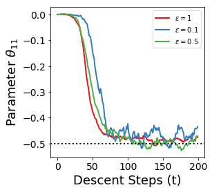
Refer to caption
Refer to caption
Figure 7: Inference for the parameters of a two-scale stochastic process using a coarse grained model. The plots show the convergence of the estimators to the truth values (dashed-lines) as the number of gradient descent steps increase, for data coming from (9).

6 Conclusion

This paper studied a class of statistical estimators for models for which the likelihood is unknown, but for which we can simulate realisations given parameter values. Our estimators are based on minimising U-statistic approximations of the maximum mean discrepancy squared. We provided several results on their asymptotic properties and robustness, as well as a novel natural-gradient descent algorithm for efficient implementation. As demonstrated first in our theory, then later in the experiments, the choice of reproducing kernel allows for great flexibility and can help us trade-off statistical efficiency with robustness.

This methodology clearly provides a rigorous approach to parametric estimation of complex black-box models for which we can only evaluate the forward map and its gradient. The natural robustness properties of these estimators make them a clear candidate for fitting models to engineering systems which are subject to intermittent sensor failures. Our theory also provides insights into the behaviour of MMD estimators for neural networks such as MMD GANs.

There are several directions in which this work could be extended. Firstly, we note this methodology can be readily applied to other continuum models such as ordinary differential equations and (stochastic) partial differential equations with noisy parameters. In these cases, adjoint based methods can be exploited to reduce the cost of computing gradients.

A second direction which is promising relates to model reduction or coarse graining, where a complex, very expensive model is replaced by a series of smaller models which are far cheaper to simulate. We believe that minimum MMD based estimators are an excellent candidate for effecting these coarse graining approaches thanks to their robustness properties.

Finally, we note that a drawback of this methodology is the poor scaling as a function of data-size. Indeed, the cost of computing MMD grows quadratically with data-size. This clearly motivates a second direction of research involving the use of cheaper approximate estimators for maximum mean discrepancy, such as (Chwialkowski etΒ al., 2015).

7 Acknowledgements

The authors are grateful to Tamara Broderick, Arthur Gretton and Dougal Sutherland for helpful discussions. FXB was supported by the EPSRC grants [EP/L016710/1, EP/R018413/1]. AB was supported by a Roth Scholarship funded by the Department of Mathematics of Imperial College London. AD and MG were supported by the Lloyds Register Foundation Programme on Data-Centric Engineering. MG was supported by the EPSRC grants [EP/J016934/3, EP/K034154/1, EP/P020720/1, EP/R018413/1], an EPSRC Established Career Fellowship, the EU grant [EU/259348]. All four authors were also supported by The Alan Turing Institute under the EPSRC grant [EP/N510129/1].

References

  • Abbati etΒ al. [2019] G.Β Abbati, P.Β Wenk, S.Β Bauer, M.Β A. Osborne, A.Β Krause, and B.Β Scholkopf. AReS and MaRS - Adversarial and MMD-Minimizing Regression for SDEs. In International Conference on Machine Learning, pages 1–10, 2019.
  • Amari [1987] S.-I. Amari. Differential Geometrical Methods in Statistics. Springer-Verlag, 1987.
  • Amari [1998] S.-I. Amari. Natural gradient works efficiently in learning. Neural Computation, 10(2):251–276, 1998.
  • Arbel etΒ al. [2018] M.Β Arbel, D.Β J. Sutherland, M.Β Binkowski, and A.Β Gretton. On gradient regularizers for MMD GANs. In Neural Information Processing Systems, pages 6700–6710, 2018.
  • Barndorff-Nielsen [1978] O.Β Barndorff-Nielsen. Information and Exponential Families in Statistical Theory. Wiley, 1978.
  • Bassetti etΒ al. [2006] F.Β Bassetti, A.Β Bodini, and E.Β Regazzini. On minimum Kantorovich distance estimators. Statistics & Probability Letters, 76:1298–1302, 2006.
  • Basu etΒ al. [2011] A.Β Basu, H.Β Shioya, and C.Β Park. Statistical Inference: The Minimum Distance Approach. CRC Press, 2011.
  • Beaumont etΒ al. [2002] M.Β A. Beaumont, W.Β Zhang, and D.Β J. Balding. Approximate Bayesian Computation in population genetics. Genetics, 162:2025–2035, 2002.
  • Berlinet and Thomas-Agnan [2004] A.Β Berlinet and C.Β Thomas-Agnan. Reproducing Kernel Hilbert Spaces in Probability and Statistics. Springer Science+Business Media, New York, 2004.
  • Bernton etΒ al. [2019] E.Β Bernton, P.Β E. Jacob, M.Β Gerber, and C.Β P. Robert. Approximate Bayesian computation with the Wasserstein distance. Journal of the Royal Statistical Society Series B: Statistical Methodology, 81(2):235–269, 2019.
  • Besag [1974] J.Β Besag. Spatial interaction and the statistical analysis of lattice systems. Journal of the Royal Statistical Society Series B: Statistical Methodology, 36(2):192–236, 1974.
  • Beskos and Roberts [2005] A.Β Beskos and G.Β O. Roberts. Exact simulation of diffusions. The Annals of Applied Probability, 15(4):2422–2444, 2005.
  • BiΕ„kowski etΒ al. [2018] M.Β BiΕ„kowski, D.Β J. Sutherland, M.Β Arbel, and A.Β Gretton. Demystifying MMD GANs. In International Conference on Learning Representation, 2018.
  • Bottou etΒ al. [2017] L.Β Bottou, M.Β Arjovsky, D.Β Lopez-Paz, and M.Β Oquab. Geometrical insights for implicit generative modeling. Braverman Readings in Machine Learning: Key Ideas from Inception to Current State, pages 229–268, 2017.
  • Briol etΒ al. [2019] F-X. Briol, C.Β J. Oates, M.Β Girolami, M.Β A. Osborne, and D.Β Sejdinovic. Probabilistic integration: A role in statistical computation? (with discussion). Statistical Science, 34(1):1–22, 2019.
  • Burago etΒ al. [2001] D.Β Burago, I.Β Burago, and S.Β Ivanov. A Course in Metric Geometry. American Mathematical Society, 2001.
  • Cameron and Pettitt [2012] E.Β Cameron and A.Β N. Pettitt. Approximate Bayesian Computation for astronomical model analysis: A case study in galaxy demographics and morphological transformation at high redshift. Monthly Notices of the Royal Astronomical Society, 425(1):44–65, 2012.
  • Campbell [1986] L.Β L. Campbell. An extended Cencov characterization of the information metric. Proceedings of the American Mathematical Society, 98(1):135–141, 1986.
  • Cencov [2000] N.Β N. Cencov. Statistical Decision Rules and Optimal Inference. NumberΒ 53. American Mathematical Society, 2000.
  • Chen and Li [2018] Y.Β Chen and W.Β Li. Natural gradient in Wasserstein statistical manifold. arXiv:1805.08380, 2018.
  • Chwialkowski etΒ al. [2015] K.Β Chwialkowski, A.Β Ramdas, D.Β Sejdinovic, and A.Β Gretton. Fast two-sample testing with analytic representations of probability measures. In Advances in Neural Information Processing Systems, pages 1981–1989, 2015.
  • Cuevas [1988] A.Β Cuevas. Qualitative robustness in abstract inference. Journal of Statistical Planning and Inference, 18(3):277–289, 1988.
  • Dawid [2007] A.Β P. Dawid. The geometry of proper scoring rules. Annals of the Institute of Statistical Mathematics, 59(1):77–93, 2007.
  • Dawid and Musio [2014] A.Β P. Dawid and Monica Musio. Theory and applications of proper scoring rules. Metron, 72(2):169–183, 2014.
  • Dick etΒ al. [2013] J.Β Dick, F.Β Y. Kuo, and I.Β H. Sloan. High-dimensional integration: The quasi-Monte Carlo way. Acta Numerica, 22(April 2013):133–288, 2013.
  • dos Santos etΒ al. [2019] C.Β N. dos Santos, Y.Β Mroueh, IΒ Padhi, and P.Β Dognin. Learning implicit generative models by matching perceptual features. arXiv:1904.02762, 2019.
  • [27] B.Β A. Dubrovin, A.Β T. Fomenko, S.Β P. Novikov, and R.Β G. Burns. Modern Geometry - Methods and Applications. Part I: The Geometry of Surfaces, Transformation Groups, and Fields. Springer.
  • Dudley [2018] R.Β M. Dudley. Real Analysis and Probability. Chapman and Hall/CRC, 2018.
  • Dziugaite etΒ al. [2015] G.Β K. Dziugaite, D.Β M. Roy, and Z.Β Ghahramani. Training generative neural networks via Maximum Mean Discrepancy optimization. In Uncertainty in Artificial Intelligence, 2015.
  • Eaton [1982] M.Β L. Eaton. A method for evaluating improper prior distributions. Statistical Decision Theory and Related Topics III, pages 329–352, 1982.
  • Erban etΒ al. [2006] R.Β Erban, I.Β G. Kevrekidis, and H.Β G. Othmer. An equation-free computational approach for extracting population-level behavior from individual-based models of biological dispersal. Physica D: Nonlinear Phenomena, 215(1):1–24, 2006.
  • Fearnhead and Prangle [2011] P.Β Fearnhead and D.Β Prangle. Constructing summary statistics for approximate Bayesian computation: semi-automatic ABC. Journal of the Royal Statistical Society B: Statistical Methodology, 74(3):419–474, 2011.
  • Fournier and Guillin [2015] N.Β Fournier and A.Β Guillin. On the rate of convergence in Wasserstein distance of the empirical measure. Probability Theory and Related Fields, 162(3-4):707–738, 2015.
  • Friedman [2012] A.Β Friedman. Stochastic Differential Equations and Applications. Courier Corporation, 2012.
  • Frogner and Poggio [2018] C.Β Frogner and T.Β Poggio. Approximate inference with Wasserstein gradient flows. arXiv:1806.04542, 2018.
  • Frogner etΒ al. [2015] C.Β Frogner, C.Β Zhang, H.Β Mobahi, M.Β Araya-Polo, and T.Β Poggio. Learning with a Wasserstein loss. In Advances in Neural Information Processing Systems, pages 2053–2061, 2015.
  • Fukumizu etΒ al. [2013] K.Β Fukumizu, L.Β Song, and A.Β Gretton. Kernel Bayes’ rule: Bayesian inference with positive definite kernels. Journal of Machine Learning Research, 14:3753–3783, 2013.
  • Garreau etΒ al. [2017] D.Β Garreau, W.Β Jitkrittum, and M.Β Kanagawa. Large sample analysis of the median heuristic. arXiv:1707.07269, 2017.
  • Genevay etΒ al. [2018] A.Β Genevay, G.Β PeyrΓ©, and M.Β Cuturi. Learning generative models with Sinkhorn divergences. In Proceedings of the Twenty-First International Conference on Artificial Intelligence and Statistics, PMLR 84, pages 1608–1617, 2018.
  • Genevay etΒ al. [2019] A.Β Genevay, L.Β Chizat, F.Β Bach, M.Β Cuturi, and G.Β PeyrΓ©. Sample complexity of Sinkhorn divergences. In International Conference on Artificial Intelligence and Statistics, 2019.
  • Girolami and Calderhead [2011] M.Β Girolami and B.Β Calderhead. Riemann manifold Langevin and Hamiltonian Monte Carlo methods. Journal of the Royal Statistical Society Series B: Statistical Methodology, 73(2):123–214, 2011.
  • Gneiting and Raftery [2007] T.Β Gneiting and A.Β E. Raftery. Strictly proper scoring rules, prediction, and estimation. Journal of the American Statistical Association, 102(477):359–378, 2007.
  • Gobet and Munos [2005] E.Β Gobet and R.Β Munos. Sensitivity analysis using Itô–Malliavin calculus and martingales, and application to stochastic optimal control. SIAM Journal on Control and Optimization, 43(5):1676–1713, 2005.
  • Godambe [1960] V.Β P. Godambe. An optimum property of regular maximum likelihood estimation. The Annals of Mathematical Statistics, 31(4):1208–1211, 1960.
  • Goodfellow etΒ al. [2014] I.Β Goodfellow, J.Β Pouget-Abadie, M.Β Mirza, B.Β Xu, D.Β Warde-Farley, S.Β Ozair, A.Β Courville, and Y.Β Bengio. Generative adversarial networks. In Advances in Neural Information Processing Systems, pages 2672–2680, 2014.
  • Gretton etΒ al. [2008] A.Β Gretton, K.Β Borgwardt, M.Β Rasch, B.Β Scholkopf, and A.Β Smola. A kernel method for the two-sample problem. Journal of Machine Learning Research, 1(157):0–43, 2008.
  • Gretton etΒ al. [2009] A.Β Gretton, K.Β Fukumizu, Z.Β Harchaoui, and B.Β K. Sriperumbudur. A fast, consistent kernel two-sample test. Advances in Neural Information Processing Systems, pages 673–681, 2009.
  • Gutmann and Hyvarinen [2012] M.Β U. Gutmann and A.Β Hyvarinen. Noise-contrastive estimation of unnormalized statistical models, with applications to natural image statistics. Journal of Machine Learning Research, 13:307–361, 2012.
  • HΓ‘jek and Johanis [2014] P.Β HΓ‘jek and M.Β Johanis. Smooth Analysis in Banach Spaces, volumeΒ 19. Walter de Gruyter GmbH & Co KG, 2014.
  • Hall [2005] A.Β R. Hall. Generalized Method of Moments. Oxford University Press, 2005.
  • Hampel [1971] F.Β R. Hampel. A general qualitative definition of robustness. The Annals of Mathematical Statistics, 42(6):1887–1896, 1971.
  • Hoeffding [1948] W.Β Hoeffding. A class of statistics with asymptotically normal distribution. The Annals of mathematical statistics, pages 293–325, 1948.
  • Hoffman etΒ al. [2013] M.Β D. Hoffman, D.Β M. Blei, C.Β Wang, and J.Β Paisley. Stochastic variational inference. Journal of Machine Learning Research, 14(1):1303–1347, 2013.
  • Huber and Ronchetti [2009] P.Β J. Huber and E.Β M. Ronchetti. Robust Statistics. Wiley, 2009.
  • HyvΓ€rinen [2006] A.Β HyvΓ€rinen. Estimation of non-normalized statistical models by score matching. Journal of Machine Learning Research, 6:695–708, 2006.
  • HyvΓ€rinen [2007] A.Β HyvΓ€rinen. Some extensions of score matching. Computational Statistics and Data Analysis, 51(5):2499–2512, 2007.
  • Jarrett [1984] R.Β G. Jarrett. Bounds and expansions for Fisher information when the moments are known. Biometrika, 71(1):101–113, 1984.
  • Jordan etΒ al. [1998] R.Β Jordan, D.Β Kinderlehrer, and F.Β Otto. The variational formulation of the Fokker–Planck equation. SIAM Journal on Mathematical Analysis, 29(1):1–17, 1998.
  • Kakade [2002] S.Β M. Kakade. A natural policy gradient. In Advances in Neural Information Processing Systems, pages 1531–1538, 2002.
  • Karakida etΒ al. [2016] R.Β Karakida, M.Β Okada, and S.-I. Amari. Adaptive natural gradient learning algorithms for unnormalized statistical models. Artificial Neural Networks and Machine Learning - ICANN, 2016.
  • Kim etΒ al. [1998] S.Β Kim, N.Β Shephard, and S.Β Chib. Stochastic volatility: likelihood inference and comparison with ARCH models. The Review of Economic Studies, 65(3):361–393, 1998.
  • Kingma and Welling [2014] D.Β P. Kingma and M.Β Welling. Auto-Encoding Variational Bayes. In International Conference on Learning Representations, 2014.
  • Krumscheid [2018] S.Β Krumscheid. Perturbation-based inference for diffusion processes: Obtaining effective models from multiscale data. Mathematical Models and Methods in Applied Sciences, 28(08):1565–1597, 2018.
  • Kunita [1997] H.Β Kunita. Stochastic Flows and Stochastic Differential Equations, volumeΒ 24. Cambridge University Press, 1997.
  • Kushner and Yin [2003] H.Β J. Kushner and G.Β G. Yin. Stochastic approximation and recursive algorithms and applications. Springer, 2003.
  • Lang [2012] S.Β Lang. Fundamentals of Differential Geometry, volume 191. Springer Science & Business Media, 2012.
  • Lehmann [1951] E.Β Lehmann. Consistency and unbiasness of certain nonparametric tests. Annals of Mathematical Statistics, 22:165–179, 1951.
  • Li etΒ al. [2017] C.-L. Li, W.-C. Chang, Y.Β Cheng, Y.Β Yang, and B.Β PΓ³czos. MMD GAN: Towards deeper understanding of moment matching network. In Advances in Neural Information Processing Systems, pages 2203–2213, 2017.
  • Li and Montufar [2018] W.Β Li and G.Β Montufar. Natural gradient via optimal transport. Information Geometry, 1(2):181–214, 2018.
  • Li etΒ al. [2015] Y.Β Li, K.Β Swersky, and R.Β Zemel. Generative Moment Matching Networks. In Proceedings of the International Conference on Machine Learning, volumeΒ 37, pages 1718–1727, 2015.
  • Lintusaari etΒ al. [2017] J.Β Lintusaari, M.Β U. Gutmann, R.Β Dutta, S.Β Kaski, and J.Β Corander. Fundamentals and recent developments in approximate Bayesian computation. Systematic Biology, 66(1):66–82, 2017.
  • Majda etΒ al. [2001] A.Β J. Majda, I.Β Timofeyev, and E.Β VandenΒ Eijnden. A mathematical framework for stochastic climate models. Communications on Pure and Applied Mathematics, 54(8):891–974, 2001.
  • Marin etΒ al. [2012] J.Β M. Marin, P.Β Pudlo, C.Β P. Robert, and R.Β J. Ryder. Approximate Bayesian computational methods. Statistics and Computing, 22(6):1167–1180, 2012.
  • Masnadi-Shirazi [2017] H.Β Masnadi-Shirazi. Strictly proper kernel scoring rules and divergences with an application to kernel two-sample hypothesis testing. arXiv:1704.02578, 2017.
  • McDiarmid [1989] C.Β McDiarmid. On the Method of Bounded Differences, pages 148–188. London Mathematical Society Lecture Note Series. Cambridge University Press, 1989.
  • Mohamed and Lakshminarayanan [2016] S.Β Mohamed and B.Β Lakshminarayanan. Learning in implicit generative models. arXiv:1610.03483v4, 2016.
  • Moller etΒ al. [2006] J.Β Moller, A.Β N. Pettitt, and R.Β Reeves. An efficient Markov Chain Monte Carlo method for distributions with intractable normalising constants. Biometrika, 93(2):451–458, 2006.
  • Montavon etΒ al. [2016] G.Β Montavon, K.-R. MΓΌller, and M.Β Cuturi. Wasserstein training of Boltzmann machines. In Advances in Neural Information Processing Systems, pages 3718–3726, 2016.
  • MontΓΊfar etΒ al. [2014] G.Β MontΓΊfar, J.Β Rauh, and N.Β Ay. On the Fisher metric of conditional probability polytopes. Entropy, 16(6):3207–3233, 2014.
  • Muller [1997] A.Β Muller. Integral probability metrics and their generating classes of functions. Advances in Applied Probability, 29(2):429–443, 1997.
  • Murphy and van der Vaart [2000] S.Β A. Murphy and A.Β W. van der Vaart. On profile likelihood. Journal of the American Statistical Association, 95(450):449–465, 2000.
  • Murray etΒ al. [2006] I.Β Murray, Z.Β Ghahramani, and D.Β J.Β C. MacKay. MCMC for doubly-intractable distributions. In Proceedings of the Twenty-Second Conference on Uncertainty in Artificial Intelligence, pages 359–366, 2006.
  • Neumeyer [2004] N.Β Neumeyer. A central limit theorem for two-sample U-processes. Statistics and Probability Letters, 67(1):73–85, 2004.
  • Nolan and Pollard [1987] D.Β Nolan and D.Β Pollard. U-Processes: Rates of convergence. Annals of Statistics, 15(2):780–799, 1987.
  • Ollivier [2018] Y.Β Ollivier. Online natural gradient as a Kalman filter. Electronic Journal of Statistics, 12(2):2930–2961, 2018.
  • Papadopoulos [2014] A.Β Papadopoulos. Metric Spaces, Convexity and Nonpositive Curvature, volumeΒ 6. European Mathematical Society, 2014.
  • Pardo [2005] L.Β Pardo. Statistical Inference Based on Divergence Measures, volume 170. Chapman and Hall/CRC, 2005.
  • Park etΒ al. [2000] H.Β Park, S-I. Amari, and K.Β Fukumizu. Adaptive natural gradient learning algorithms for various stochastic models. Neural Networks, 13(7):755–764, 2000.
  • Park etΒ al. [2015] M.Β Park, W.Β Jitkrittum, and D.Β Sejdinovic. K2-ABC: approximate Bayesian computation with kernel embeddings. Proceedings of the 19th International Conference on Artificial Intelligence and Statistics, PMLR 51:398–407, 2015.
  • Pavliotis and Stuart [2008] G.Β Pavliotis and A.Β Stuart. Multiscale Methods: Averaging and Homogenization. Springer Science & Business Media, 2008.
  • Pavliotis and Stuart [2007] G.Β A. Pavliotis and A.Β M. Stuart. Parameter estimation for multiscale diffusions. Journal of Statistical Physics, 127(4):741–781, 2007.
  • Prangle [2017] D.Β Prangle. gk: An R Package for the g-and-k and generalised g-and-h Distributions. arXiv:1706.06889, 2017.
  • Ramdas etΒ al. [2015] A.Β Ramdas, S.Β J. Reddi, A.Β Singh, and L.Β Wasserman. Adaptivity and computation-statistics tradeoffs for kernel and distance based high-dimensional two sample testing. arXiv:1508.00655, 2015.
  • Reddi etΒ al. [2015] S.Β J. Reddi, A.Β Ramdas, B.Β Poczos, A.Β Singh, and L.Β Wasserman. On the high-dimensional power of linear-time kernel two-sample testing under mean-difference alternatives. In International Conference on Artificial Intelligence and Statistics, pages 772–780, 2015.
  • Ren etΒ al. [2016] Y.Β Ren, J.Β Li, Y.Β Luo, and J.Β Zhu. Conditional generative moment-matching networks. In Advances in Neural Information Processing Systems, pages 2928–2936, 2016.
  • Robbins and Monro [1985] H.Β Robbins and S.Β Monro. A stochastic approximation method. In Herbert Robbins Selected Papers, pages 102–109. Springer, 1985.
  • Romano etΒ al. [2018] Y.Β Romano, M.Β Sesia, and E.Β J. CandΓ¨s. Deep knockoffs. arXiv:1811.06687, 2018.
  • Sanjabi etΒ al. [2018] M.Β Sanjabi, J.Β Ba, M.Β Razaviyayn, and J.Β D. Lee. On the convergence and robustness of training GANs with regularized optimal transport. In Advances in Neural Information Processing Systems, pages 7088–7098, 2018.
  • Sriperumbudur [2016] B.Β K. Sriperumbudur. On the optimal estimation of probability measures in weak and strong topologies. Bernoulli, 22(3):1839–1893, 2016.
  • Sriperumbudur etΒ al. [2010] B.Β K. Sriperumbudur, A.Β Gretton, K.Β Fukumizu, B.Β SchΓΆlkopf, and G.Β R.Β G. Lanckriet. Hilbert space embeddings and metrics on probability measures. Journal of Machine Learning Research, 11, 2010.
  • Sriperumbudur etΒ al. [2012] B.Β K. Sriperumbudur, K.Β Fukumizu, A.Β Gretton, B.Β SchΓΆlkopf, and .Β RΒ G Lanckriet. On the empirical estimation of integral probability metrics. Electronic Journal of Statistics, 6:1550–1599, 2012.
  • Stein and Nossek [2017] M.Β S. Stein and J.Β A. Nossek. A pessimistic approximation for the Fisher information measure. IEEE Transactions on Signal Processing, 65(2):386–396, 2017.
  • Steinwart and Christmann [2008] I.Β Steinwart and A.Β Christmann. Support Vector Machines. Springer, 2008.
  • Steinwart and Ziegel [2017] I.Β Steinwart and J.Β F. Ziegel. Strictly proper kernel scores and characteristic kernels on compact spaces. arXiv:1712.05279, 2017.
  • Sutherland etΒ al. [2017] D.Β J. Sutherland, H.-Y. Tung, H.Β Strathmann, S.Β De, A.Β Ramdas, A.Β Smola, and A.Β Gretton. Generative models and model criticism via optimized maximum mean discrepancy. In Proceedings of the International Conference on Learning Representation, 2017.
  • Tzen and Raginsky [2019] B.Β Tzen and M.Β Raginsky. Neural stochastic differential equations: Deep latent gaussian models in the diffusion limit. arXiv preprint arXiv:1905.09883, 2019.
  • vanΒ der Vaart [1998] A.W. vanΒ der Vaart. Asymptotic Statistics. Cambridge University Press, 1998.
  • Varin etΒ al. [2011] C.Β Varin, N.Β Reid, and D.Β Firth. An overview of composite likelihood methods. Statistica Sinica, 21:5–42, 2011.
  • Volterra [1926] V.Β Volterra. Fluctuations in the abundance of a species considered mathematically. Nature, 118(2972):558–560, 1926.
  • Weed and Bach [2017] J.Β Weed and F.Β Bach. Sharp asymptotic and finite-sample rates of convergence of empirical measures in Wasserstein distance. Bernoulli (to appear), 2017.
  • Weed and Berthet [2019] J.Β Weed and Q.Β Berthet. Estimation of smooth densities in Wasserstein distance. arXiv:1902.01778, 2019.
  • Weinan [2011] E.Β Weinan. Principles of Multiscale Modeling. Cambridge University Press, 2011.
  • Wood [2010] S.Β N. Wood. Statistical inference for noisy nonlinear ecological dynamic systems. Nature, 466(7310):1102–1104, 2010.
  • Zawadzki and Lahaie [2015] E.Β Zawadzki and S.Β Lahaie. Nonparametric scoring rules. In Proceedings of the 29th Conference on Artificial Intelligence (AAAI 2015), pages 3635–3641, 2015.

Supplementary Material for β€œStatistical Inference for Generative Models with Maximum Mean Discrepancy”

The supplementary materials are structured as follows. Section A provides further discussion on the geometry induced by MMD on parametric families of probability distributions, and in particular derives the corresponding metric tensor, gradient flow and geodesics. Section B contains all the proofs of results in the paper, including asymptotic results and results on robustness. Section C contains the derivation of important quantities for the Gaussian models. Finally, Section D contains further details on the numerical experiments.

Appendix A Geometry of the MMD Statistical Manifold

In this appendix we complement Section 2 and provide additional details on the Riemmanian manifold induced by the MMD metric.

A.1 Identification of the Information Metric Tensor

Identifying β„™ΞΈsubscriptβ„™πœƒ\mathbb{P}_{\theta} as the pushforward GΞΈ#β€‹π•ŒsuperscriptsubscriptπΊπœƒ#π•ŒG_{\theta}^{\#}\mathbb{U}, we have:

MMD2(β„™Ξ±||β„™Ξ²)\displaystyle{\operatorname*{\text{MMD}}}^{2}(\mathbb{P}_{\alpha}||\mathbb{P}_{\beta}) =βˆ«π’°βˆ«π’°k​(Gα​(u),Gα​(v))β€‹π•Œβ€‹(d​u)β€‹π•Œβ€‹(d​v)βˆ’2β€‹βˆ«π’°βˆ«π’°k​(Gα​(u),Gβ​(v))β€‹π•Œβ€‹(d​u)β€‹π•Œβ€‹(d​v)absentsubscript𝒰subscriptπ’°π‘˜subscript𝐺𝛼𝑒subscriptπΊπ›Όπ‘£π•Œdπ‘’π•Œd𝑣2subscript𝒰subscriptπ’°π‘˜subscript𝐺𝛼𝑒subscriptπΊπ›½π‘£π•Œdπ‘’π•Œd𝑣\displaystyle=\int_{\mathcal{U}}\int_{\mathcal{U}}k(G_{\alpha}(u),G_{\alpha}(v))\mathbb{U}(\mathrm{d}u)\mathbb{U}(\mathrm{d}v)-2\int_{\mathcal{U}}\int_{\mathcal{U}}k(G_{\alpha}(u),G_{\beta}(v))\mathbb{U}(\mathrm{d}u)\mathbb{U}(\mathrm{d}v)
+βˆ«π’°βˆ«π’°k​(Gβ​(u),Gβ​(v))β€‹π•Œβ€‹(d​u)β€‹π•Œβ€‹(d​v)subscript𝒰subscriptπ’°π‘˜subscript𝐺𝛽𝑒subscriptπΊπ›½π‘£π•Œdπ‘’π•Œd𝑣\displaystyle+\int_{\mathcal{U}}\int_{\mathcal{U}}k(G_{\beta}(u),G_{\beta}(v))\mathbb{U}(\mathrm{d}u)\mathbb{U}(\mathrm{d}v)

Taking the derivative with respect to α𝛼\alpha and β𝛽\beta, and noticing that:

βˆ‚Ξ²kβˆ‚Ξ±jk​(Gα​(u),Gβ​(v))subscriptsuperscriptπ›½π‘˜subscriptsuperscriptπ›Όπ‘—π‘˜subscript𝐺𝛼𝑒subscript𝐺𝛽𝑣\displaystyle\partial_{\beta^{k}}\partial_{\alpha^{j}}k(G_{\alpha}(u),G_{\beta}(v)) =βˆ‘l,iβˆ‚2lβˆ‚1ik​(Gα​(u),Gβ​(v))β€‹βˆ‚Ξ±jGΞ±i​(u)β€‹βˆ‚Ξ²kGΞ²l​(v)absentsubscript𝑙𝑖subscriptsuperscript2𝑙subscriptsuperscript1π‘–π‘˜subscript𝐺𝛼𝑒subscript𝐺𝛽𝑣subscriptsuperscript𝛼𝑗superscriptsubscript𝐺𝛼𝑖𝑒subscriptsuperscriptπ›½π‘˜superscriptsubscript𝐺𝛽𝑙𝑣\displaystyle=\sum_{l,i}\partial_{2^{l}}\partial_{1^{i}}k(G_{\alpha}(u),G_{\beta}(v))\partial_{\alpha^{j}}G_{\alpha}^{i}(u)\partial_{\beta^{k}}G_{\beta}^{l}(v)
=(βˆ‡Ξ±Gα​(u)βŠ€β€‹βˆ‡2βˆ‡1⁑k​(Gα​(u),Gβ​(v))β€‹βˆ‡Ξ²Gβ​(v))j​kabsentsubscriptsubscriptβˆ‡π›Όsubscript𝐺𝛼superscript𝑒topsubscriptβˆ‡2subscriptβˆ‡1π‘˜subscript𝐺𝛼𝑒subscript𝐺𝛽𝑣subscriptβˆ‡π›½subscriptπΊπ›½π‘£π‘—π‘˜\displaystyle=\big{(}\nabla_{\alpha}G_{\alpha}(u)^{\top}\nabla_{2}\nabla_{1}k(G_{\alpha}(u),G_{\beta}(v))\nabla_{\beta}G_{\beta}(v)\big{)}_{jk}

which yields the expression for the information metric associated to the MMD2superscriptMMD2\text{MMD}^{2} divergence. Let β„‹β„‹\mathcal{H} be a Hilbert space viewed as a Hilbert manifold. As usual we identify the tangent spaces Tp​ℋ≅ℋsubscript𝑇𝑝ℋℋT_{p}\mathcal{H}\cong\mathcal{H}, and the Riemannian metric is m​(f,g)=⟨f,gβŸ©π‘šπ‘“π‘”π‘“π‘”m(f,g)=\langle f,g\rangle for any f,gβˆˆβ„‹π‘“π‘”β„‹f,g\in\mathcal{H}. Let Ξ¨:Sβ†’β„‹:Ψ→𝑆ℋ\Psi:S\to\mathcal{H} be a differentiable injective immersion (i.e., its derivative is injective), from a finite-dimensional manifold S𝑆S. Then ΨΨ\Psi induces a Riemannian structure on S𝑆S given by the pull-back Riemannian metric g=Ξ¨βˆ—β€‹m𝑔superscriptΞ¨π‘šg=\Psi^{*}m. If xisuperscriptπ‘₯𝑖x^{i} are local coordinates on S𝑆S, and βˆ‚xisubscriptsuperscriptπ‘₯𝑖\partial_{x^{i}} is the associated local basis of vector fields, then the components of g𝑔g are defined by

gi​j=g​(βˆ‚xi,βˆ‚xj)=m​(d​Ψ​(βˆ‚xi),d​Ψ​(βˆ‚xj)),subscript𝑔𝑖𝑗𝑔subscriptsuperscriptπ‘₯𝑖subscriptsuperscriptπ‘₯π‘—π‘šπ‘‘Ξ¨subscriptsuperscriptπ‘₯𝑖𝑑Ψsubscriptsuperscriptπ‘₯𝑗\displaystyle g_{ij}=g(\partial_{x^{i}},\partial_{x^{j}})=m\big{(}d\Psi(\partial_{x^{i}}),d\Psi(\partial_{x^{j}})\big{)},

where d​Ψ:T​Sβ†’T​ℋ:𝑑Ψ→𝑇𝑆𝑇ℋd\Psi:TS\to T\mathcal{H} is the differential/tangent map (here T​S𝑇𝑆TS denotes the tangent bundle of S𝑆S, or, roughly, the set of vectors tangent to S𝑆S). When S𝑆S is an open subset of ℝnsuperscriptℝ𝑛\mathbb{R}^{n}, since the Frechet partial derivative βˆ‡xjΨ​(x)subscriptβˆ‡superscriptπ‘₯𝑗Ψπ‘₯\nabla_{x^{j}}\Psi(x) is the derivative of the function t↦Ψ​(x1,…,xjβˆ’1,t,xj+1,…,xn)maps-to𝑑Ψsuperscriptπ‘₯1…superscriptπ‘₯𝑗1𝑑superscriptπ‘₯𝑗1…superscriptπ‘₯𝑛t\mapsto\Psi(x^{1},\ldots,x^{j-1},t,x^{j+1},\ldots,x^{n}), of the curve t↦(x1,…,xjβˆ’1,t,xj+1,…,xn)maps-to𝑑superscriptπ‘₯1…superscriptπ‘₯𝑗1𝑑superscriptπ‘₯𝑗1…superscriptπ‘₯𝑛t\mapsto(x^{1},\ldots,x^{j-1},t,x^{j+1},\ldots,x^{n}) is precisely the curve tangent to the vector βˆ‚xj|xevaluated-atsubscriptsuperscriptπ‘₯𝑗π‘₯\partial_{x^{j}}|_{x}, we have βˆ‡xjΞ¨=d​Ψ​(βˆ‚xj)subscriptβˆ‡superscriptπ‘₯𝑗Ψ𝑑Ψsubscriptsuperscriptπ‘₯𝑗\nabla_{x^{j}}\Psi=d\Psi(\partial_{x^{j}}) (see (Lang, 2012) page 28). Hence gi​j=m​(βˆ‡xiΞ¨,βˆ‡xjΞ¨)subscriptπ‘”π‘–π‘—π‘šsubscriptβˆ‡superscriptπ‘₯𝑖Ψsubscriptβˆ‡superscriptπ‘₯𝑗Ψg_{ij}=m\big{(}\nabla_{x^{i}}\Psi,\nabla_{x^{j}}\Psi\big{)}.

Note that if ΨΨ\Psi is not an immersion, the pullback Riemannian metric will in general just be a degenerate quadratic form rather than a positive definite one.

Let S𝑆S be a statistical manifold, i.e., x∈Sπ‘₯𝑆x\in S is associated to a probability measure Pxsubscript𝑃π‘₯P_{x} (we assume the map x↦Pxmaps-toπ‘₯subscript𝑃π‘₯x\mapsto P_{x} is a bijection). We can define a divergence on S𝑆S by D​(PΞ±,PΞ²)=‖Ψ​(Ξ±)βˆ’Ξ¨β€‹(Ξ²)β€–2𝐷subscript𝑃𝛼subscript𝑃𝛽superscriptnormΨ𝛼Ψ𝛽2D\big{(}P_{\alpha},P_{\beta}\big{)}=\|\Psi(\alpha)-\Psi(\beta)\|^{2}, which is the pull-back of the square-metric (f,g)↦‖fβˆ’gβ€–2maps-to𝑓𝑔superscriptnorm𝑓𝑔2(f,g)\mapsto\|f-g\|^{2} on β„‹β„‹\mathcal{H} induced by the inner product. The corresponding information metric has components Ii​jsubscript𝐼𝑖𝑗I_{ij} in a local coordinate chart given by

Ii​jsubscript𝐼𝑖𝑗\displaystyle I_{ij} =βˆ’βˆ‚βˆ‚Ξ±kβ€‹βˆ‚Ξ²j​D​(p​(Ξ±),p​(Ξ²))|Ξ±=Ξ²=ΞΈ=2β€‹βˆ‚Ξ²jβˆ‚Ξ±kβŸ¨Ξ¨β€‹(Ξ±),Ψ​(Ξ²)⟩|Ξ±=Ξ²=ΞΈ.absentevaluated-atsuperscriptπ›Όπ‘˜superscriptπ›½π‘—π·π‘π›Όπ‘π›½π›Όπ›½πœƒevaluated-at2subscriptsuperscript𝛽𝑗subscriptsuperscriptπ›Όπ‘˜Ξ¨π›ΌΞ¨π›½π›Όπ›½πœƒ\displaystyle=-\frac{\partial}{\partial\alpha^{k}\partial{\beta^{j}}}D\big{(}p(\alpha),p(\beta)\big{)}|_{\alpha=\beta=\theta}=2\partial_{\beta^{j}}\partial_{\alpha^{k}}\langle\Psi(\alpha),\Psi(\beta)\rangle|_{\alpha=\beta=\theta}.

Suppose now that β„‹ksubscriptβ„‹π‘˜\mathcal{H}_{k} is a RKHS, and ΨΨ\Psi is defined as the mean-embedding. Then

βŸ¨Ξ¨β€‹(Ξ±),Ψ​(Ξ²)βŸ©Ξ¨π›ΌΞ¨π›½\displaystyle\langle\Psi(\alpha),\Psi(\beta)\rangle =βˆ«π’³βˆ«π’³k​(x,y)​Pα​(d​x)​Pβ​(d​y).absentsubscript𝒳subscriptπ’³π‘˜π‘₯𝑦subscript𝑃𝛼dπ‘₯subscript𝑃𝛽d𝑦\displaystyle=\int_{\mathcal{X}}\int_{\mathcal{X}}k(x,y)P_{\alpha}(\mathrm{d}x)P_{\beta}(\mathrm{d}y).

In particular if the measures in S𝑆S can be written as either PΞ±=GΞ±#​μsubscript𝑃𝛼superscriptsubscript𝐺𝛼#πœ‡P_{\alpha}=G_{\alpha}^{\#}\mu, or Pα​(d​x)=pα​(x)​μ​(d​x)subscript𝑃𝛼dπ‘₯subscript𝑝𝛼π‘₯πœ‡dπ‘₯P_{\alpha}(\mathrm{d}x)=p_{\alpha}(x)\mu(\mathrm{d}x) for some fixed measure ΞΌπœ‡\mu, then βˆ‚Ξ²jβˆ‚Ξ±kβŸ¨Ξ¨β€‹(Ξ±),Ψ​(Ξ²)⟩|Ξ±=Ξ²=ΞΈ=βŸ¨βˆ‚ΞΈjΨ​(ΞΈ),βˆ‚ΞΈkΨ​(ΞΈ)⟩evaluated-atsubscriptsuperscript𝛽𝑗subscriptsuperscriptπ›Όπ‘˜Ξ¨π›ΌΞ¨π›½π›Όπ›½πœƒsubscriptsuperscriptπœƒπ‘—Ξ¨πœƒsubscriptsuperscriptπœƒπ‘˜Ξ¨πœƒ\partial_{\beta^{j}}\partial_{\alpha^{k}}\langle\Psi(\alpha),\Psi(\beta)\rangle|_{\alpha=\beta=\theta}=\langle\partial_{\theta^{j}}\Psi(\theta),\partial_{\theta^{k}}\Psi(\theta)\rangle and we recover the pullback Riemannian metric.

A.2 Geodesics of the MMD metric

The following result summarises the properties of the geodesics induced by the MMD metric on 𝒫ksubscriptπ’«π‘˜\mathcal{P}_{k}.

Proposition 11 (The MMD Information Metric).

Suppose that kπ‘˜k is a characteristic kernel with a bounded continuous derivative and that assumptions (i)-(iv) stated above hold. If the matrix g​(ΞΈ)=(gi​j​(ΞΈ))i,j=1,…,pπ‘”πœƒsubscriptsubscriptπ‘”π‘–π‘—πœƒformulae-sequence𝑖𝑗1…𝑝g(\theta)=(g_{ij}(\theta))_{i,j=1,\ldots,p} is positive definite on ΘΘ\Theta, then the MMD metric on 𝒫ksubscriptπ’«π‘˜\mathcal{P}_{k} induces a Riemannian geometry (Θ,g)Ξ˜π‘”(\Theta,g) on ΘΘ\Theta. The metric induced on ΘΘ\Theta is given by

dM​M​D2​(ΞΈ|ΞΈβ€²)superscriptsubscript𝑑𝑀𝑀𝐷2conditionalπœƒsuperscriptπœƒβ€²\displaystyle d_{MMD}^{2}(\theta|\theta^{\prime}) =infθ​(t)∈C1​(0,1)[∫01ΞΈΛ™(t)⊀g(ΞΈ)ΞΈΛ™(t)dt:ΞΈ(0)=ΞΈ,ΞΈ(1)=ΞΈβ€²],\displaystyle=\inf_{\theta(t)\in C^{1}(0,1)}\left[\int_{0}^{1}\dot{\theta}(t)^{\top}g(\theta)\dot{\theta}(t)dt:\theta(0)=\theta,\theta(1)=\theta^{\prime}\right], (11)

for all ΞΈ,ΞΈβ€²βˆˆΞ˜πœƒsuperscriptπœƒβ€²Ξ˜\theta,\theta^{\prime}\in\Theta. Geodesics in (Θ,g)Ξ˜π‘”(\Theta,g) are given by infimisers by (11) and satisfy the following system of ODEs Dubrovin etΒ al. :

θ˙​(t)βˆ’gβˆ’1​(θ​(t))​S​(t)=0Λ™πœƒπ‘‘superscript𝑔1πœƒπ‘‘π‘†π‘‘0\displaystyle\dot{\theta}(t)-g^{-1}(\theta(t))S(t)=0 (12)
S˙​(t)βˆ’12​S​(t)βŠ€β€‹βˆ‡ΞΈg​(θ​(t))βˆ’1​S​(t)=0.˙𝑆𝑑12𝑆superscript𝑑topsubscriptβˆ‡πœƒπ‘”superscriptπœƒπ‘‘1𝑆𝑑0\displaystyle\dot{S}(t)-\frac{1}{2}S(t)^{\top}\nabla_{\theta}g(\theta(t))^{-1}S(t)=0.

Sufficient conditions for g𝑔g being positive definite need to be verified on a case by case basis. Since (𝒫k,MMD)subscriptπ’«π‘˜MMD(\mathcal{P}_{k},\operatorname*{\text{MMD}}) is a length space (Papadopoulos, 2014; Burago etΒ al., 2001), it follows immediately that geodesics in this metric is via teleportation of mass, i.e. a geodesic connecting β„™1subscriptβ„™1\mathbb{P}_{1} and β„™2subscriptβ„™2\mathbb{P}_{2} in 𝒫ksubscriptπ’«π‘˜\mathcal{P}_{k} is defined by β„™t=(1βˆ’t)​ℙ1+t​ℙ2,t∈[0,1]formulae-sequencesubscriptℙ𝑑1𝑑subscriptβ„™1𝑑subscriptβ„™2𝑑01\mathbb{P}_{t}=(1-t)\mathbb{P}_{1}+t\mathbb{P}_{2},t\in[0,1]. This will not be the case for (Θ,g)Ξ˜π‘”(\Theta,g) as geodesics θ​(t)πœƒπ‘‘\theta(t) must be constrained to ensure that ℙθ​(t)βˆˆπ’«Ξ˜subscriptβ„™πœƒπ‘‘subscriptπ’«Ξ˜\mathbb{P}_{\theta(t)}\in\mathcal{P}_{\Theta}.

Appendix B Proofs of Main Results

In this appendix, we give the proofs of all lemmas, propositions and theorems in the main text.

B.1 Proof of Theorem 1

Before moving on to Theorem 1, we show the following result, which proves that the there is a uniform bound between the different versions of the MMD discrepancy. First, for convenience we define the following approximation to MMD between a measure β„™β„™\mathbb{P} and a empirical measure β„šm​(d​y)=1mβ€‹βˆ‘i=1mΞ΄yi​(d​y)superscriptβ„šπ‘šd𝑦1π‘šsuperscriptsubscript𝑖1π‘šsubscript𝛿subscript𝑦𝑖d𝑦\mathbb{Q}^{m}(\mathrm{d}y)=\frac{1}{m}\sum_{i=1}^{m}\delta_{y_{i}}(\mathrm{d}y):

MMDU2(β„™||β„šm)\displaystyle{\operatorname*{\text{MMD}}}_{U}^{2}(\mathbb{P}||\mathbb{Q}^{m}) =βˆ«π’³βˆ«π’³k​(x,y)​ℙ​(d​x)​ℙ​(d​y)βˆ’2mβ€‹βˆ«π’³βˆ‘i=1mk​(x,yi)​ℙ​(d​x)+1m​(mβˆ’1)β€‹βˆ‘iβ‰ iβ€²k​(yi,yiβ€²).absentsubscript𝒳subscriptπ’³π‘˜π‘₯𝑦ℙdπ‘₯β„™d𝑦2π‘šsubscript𝒳superscriptsubscript𝑖1π‘šπ‘˜π‘₯subscript𝑦𝑖ℙdπ‘₯1π‘šπ‘š1subscript𝑖superscriptπ‘–β€²π‘˜subscript𝑦𝑖subscript𝑦superscript𝑖′\displaystyle=\int_{\mathcal{X}}\int_{\mathcal{X}}k(x,y)\mathbb{P}(\mathrm{d}x)\mathbb{P}(\mathrm{d}y)-\frac{2}{m}\int_{\mathcal{X}}\sum_{i=1}^{m}k(x,y_{i})\mathbb{P}(\mathrm{d}x)+\frac{1}{m(m-1)}\sum_{i\neq i^{\prime}}k(y_{i},y_{i^{\prime}}).

Note that if {yj}j=1mβ€‹βˆΌIIDβ„šsuperscriptsubscriptsubscript𝑦𝑗𝑗1π‘šIIDsimilar-toβ„š\{y_{j}\}_{j=1}^{m}\operatorname*{\overset{\scriptscriptstyle\text{IID}}{\scriptscriptstyle\sim}}\mathbb{Q} then 𝔼[MMDU2(β„™||β„šm)]=MMD2(β„™||β„š)\mathbb{E}[{\operatorname*{\text{MMD}}}_{U}^{2}(\mathbb{P}||\mathbb{Q}^{m})]={\operatorname*{\text{MMD}}}^{2}(\mathbb{P}||\mathbb{Q}).

Lemma 2.

Suppose that kπ‘˜k is bounded, then for any two β„™,β„šβˆˆπ’«k​(𝒳)β„™β„šsubscriptπ’«π‘˜π’³\mathbb{P},\mathbb{Q}\in\mathcal{P}_{k}(\mathcal{X}) and empirical distribution β„šm=1mβ€‹βˆ‘i=1mΞ΄yjsuperscriptβ„šπ‘š1π‘šsuperscriptsubscript𝑖1π‘šsubscript𝛿subscript𝑦𝑗\mathbb{Q}^{m}=\frac{1}{m}\sum_{i=1}^{m}\delta_{y_{j}} in 𝒫k​(𝒳)subscriptπ’«π‘˜π’³\mathcal{P}_{k}(\mathcal{X}) made of independently and identically distributed realisations of β„šβ„š\mathbb{Q}, we have: |MMDU2(β„™||β„šm)βˆ’MMD2(β„™||β„šm)|≀2mβˆ’1supxβˆˆπ’³k(x,x)\left|{\operatorname*{\text{MMD}}}^{2}_{U}(\mathbb{P}||\mathbb{Q}^{m})-{\operatorname*{\text{MMD}}}^{2}(\mathbb{P}||\mathbb{Q}^{m})\right|\leq 2m^{-1}\sup_{x\in\mathcal{X}}k(x,x) and:

MMD2(β„™||β„š)\displaystyle{\operatorname*{\text{MMD}}}^{2}(\mathbb{P}||\mathbb{Q}) =𝔼[MMD2(β„™||β„šm)]+mβˆ’1(βˆ«π’³βˆ«π’³k(x,y)β„š(dx)β„š(dy)βˆ’βˆ«π’³k(x,x)β„š(dx)).\displaystyle=\mathbb{E}[{\operatorname*{\text{MMD}}}^{2}(\mathbb{P}||\mathbb{Q}^{m})]+m^{-1}\left(\int_{\mathcal{X}}\int_{\mathcal{X}}k(x,y)\mathbb{Q}(\mathrm{d}x)\mathbb{Q}(\mathrm{d}y)-\int_{\mathcal{X}}k(x,x)\mathbb{Q}(\mathrm{d}x)\right).

Similarly, when computing the MMD squared between β„šmsuperscriptβ„šπ‘š\mathbb{Q}^{m} and β„™n=1nβ€‹βˆ‘i=1nΞ΄xiβˆˆπ’«k​(𝒳)superscriptℙ𝑛1𝑛superscriptsubscript𝑖1𝑛subscript𝛿subscriptπ‘₯𝑖subscriptπ’«π‘˜π’³\mathbb{P}^{n}=\frac{1}{n}\sum_{i=1}^{n}\delta_{x_{i}}\in\mathcal{P}_{k}(\mathcal{X}) (made out of IID realisations from β„™β„™\mathbb{P}) |MMDU,U2(β„™n||β„šm)βˆ’MMD2(β„™n||β„šm)|≀2(mβˆ’1+nβˆ’1)supxβˆˆπ’³k(x,x)\left|{\operatorname*{\text{MMD}}}^{2}_{U,U}(\mathbb{P}^{n}||\mathbb{Q}^{m})-{\operatorname*{\text{MMD}}}^{2}(\mathbb{P}^{n}||\mathbb{Q}^{m})\right|\leq 2\left(m^{-1}+n^{-1}\right)\sup_{x\in\mathcal{X}}k(x,x), and similarly:

MMD2(β„™||β„š)\displaystyle{\operatorname*{\text{MMD}}}^{2}(\mathbb{P}||\mathbb{Q}) =𝔼[MMD2(β„™n||β„šm)]+(mβˆ’1+nβˆ’1)(βˆ«π’³βˆ«π’³k(x,y)β„š(dx)β„š(dy)βˆ’βˆ«π’³k(x,x)β„š(dx)).\displaystyle=\mathbb{E}[{\operatorname*{\text{MMD}}}^{2}(\mathbb{P}^{n}||\mathbb{Q}^{m})]+\left(m^{-1}+n^{-1}\right)\left(\int_{\mathcal{X}}\int_{\mathcal{X}}k(x,y)\mathbb{Q}(\mathrm{d}x)\mathbb{Q}(\mathrm{d}y)-\int_{\mathcal{X}}k(x,x)\mathbb{Q}(\mathrm{d}x)\right).
Proof.

We see that

MMDU2(β„™||β„šm)βˆ’MMD2(β„™||β„šm)\displaystyle{\operatorname*{\text{MMD}}}^{2}_{U}(\mathbb{P}||\mathbb{Q}^{m})-{\operatorname*{\text{MMD}}}^{2}(\mathbb{P}||\mathbb{Q}^{m})
=(m​(mβˆ’1))βˆ’1β€‹βˆ‘iβ‰ jk​(yi,yj)βˆ’mβˆ’2β€‹βˆ‘i=1mβˆ‘j=1mk​(yi,yj)absentsuperscriptπ‘šπ‘š11subscriptπ‘–π‘—π‘˜subscript𝑦𝑖subscript𝑦𝑗superscriptπ‘š2superscriptsubscript𝑖1π‘šsuperscriptsubscript𝑗1π‘šπ‘˜subscript𝑦𝑖subscript𝑦𝑗\displaystyle=(m(m-1))^{-1}\sum_{i\neq j}k(y_{i},y_{j})-m^{-2}\sum_{i=1}^{m}\sum_{j=1}^{m}k(y_{i},y_{j})
=(m​(mβˆ’1))βˆ’1​(1βˆ’(m​(mβˆ’1))​mβˆ’2)β€‹βˆ‘iβ‰ jk​(yi,yj)βˆ’mβˆ’2β€‹βˆ‘i=1mk​(yi,yi)absentsuperscriptπ‘šπ‘š111π‘šπ‘š1superscriptπ‘š2subscriptπ‘–π‘—π‘˜subscript𝑦𝑖subscript𝑦𝑗superscriptπ‘š2superscriptsubscript𝑖1π‘šπ‘˜subscript𝑦𝑖subscript𝑦𝑖\displaystyle=(m(m-1))^{-1}(1-(m(m-1))m^{-2})\sum_{i\neq j}k(y_{i},y_{j})-m^{-2}\sum_{i=1}^{m}k(y_{i},y_{i})
=mβˆ’1​((m​(mβˆ’1))βˆ’1β€‹βˆ‘iβ‰ jk​(yi,yj)βˆ’mβˆ’1β€‹βˆ‘i=1mk​(yi,yi)).absentsuperscriptπ‘š1superscriptπ‘šπ‘š11subscriptπ‘–π‘—π‘˜subscript𝑦𝑖subscript𝑦𝑗superscriptπ‘š1superscriptsubscript𝑖1π‘šπ‘˜subscript𝑦𝑖subscript𝑦𝑖\displaystyle=m^{-1}\Big{(}(m(m-1))^{-1}\sum_{i\neq j}k(y_{i},y_{j})-m^{-1}\sum_{i=1}^{m}k(y_{i},y_{i})\Big{)}.

Since the kernel is bounded, it follows that |MMDU2(β„™||β„šm)βˆ’MMD2(β„™||β„šm)|≀2mβˆ’1supxβˆˆπ’³k(x,x)\left|{\operatorname*{\text{MMD}}}^{2}_{U}(\mathbb{P}||\mathbb{Q}^{m})-{\operatorname*{\text{MMD}}}^{2}(\mathbb{P}||\mathbb{Q}^{m})\right|\leq 2m^{-1}\sup_{x\in\mathcal{X}}k(x,x) as required. The second statement follows in a similar fashion and from the fact that MMDU2subscriptsuperscriptMMD2π‘ˆ{\operatorname*{\text{MMD}}}^{2}_{U} is an unbiased estimator of MMD2superscriptMMD2{\operatorname*{\text{MMD}}}^{2}. Similarly for the discrepancy MMDU,U2subscriptsuperscriptMMD2π‘ˆπ‘ˆ{\operatorname*{\text{MMD}}}^{2}_{U,U}:

MMDU,U2(β„™n||β„šm)βˆ’MMD2(β„™n||β„šm)\displaystyle{\operatorname*{\text{MMD}}}^{2}_{U,U}(\mathbb{P}^{n}||\mathbb{Q}^{m})-{\operatorname*{\text{MMD}}}^{2}(\mathbb{P}^{n}||\mathbb{Q}^{m}) =mβˆ’1(m(mβˆ’1))βˆ’1βˆ‘iβ‰ jk(yi,yj)βˆ’mβˆ’1βˆ‘i=1mk(yi,yi))\displaystyle=m^{-1}(m(m-1))^{-1}\sum_{i\neq j}k(y_{i},y_{j})-m^{-1}\sum_{i=1}^{m}k(y_{i},y_{i}))
+nβˆ’1​((n​(nβˆ’1))βˆ’1β€‹βˆ‘iβ‰ jk​(xi,xj)βˆ’nβˆ’1β€‹βˆ‘i=1nk​(xi,xi)),superscript𝑛1superscript𝑛𝑛11subscriptπ‘–π‘—π‘˜subscriptπ‘₯𝑖subscriptπ‘₯𝑗superscript𝑛1superscriptsubscript𝑖1π‘›π‘˜subscriptπ‘₯𝑖subscriptπ‘₯𝑖\displaystyle\quad+n^{-1}((n(n-1))^{-1}\sum_{i\neq j}k(x_{i},x_{j})-n^{-1}\sum_{i=1}^{n}k(x_{i},x_{i})),

so |MMDU,U2(β„™n||β„šm)βˆ’MMD2(β„™n||β„šm)|≀2(mβˆ’1+nβˆ’1)supxβˆˆπ’³k(x,x)\left|{\operatorname*{\text{MMD}}}^{2}_{U,U}(\mathbb{P}^{n}||\mathbb{Q}^{m})-{\operatorname*{\text{MMD}}}^{2}(\mathbb{P}^{n}||\mathbb{Q}^{m})\right|\leq 2(m^{-1}+n^{-1})\sup_{x\in\mathcal{X}}k(x,x) and the final equation holds similarly. ∎

We now establish conditions under which a minimiser of the empirical loss always exists.

Lemma 3.

Suppose that the kernel kπ‘˜k is continuous and bounded and that the map ΞΈβ†’Gθ​(u)β†’πœƒsubscriptπΊπœƒπ‘’\theta\rightarrow G_{\theta}(u) continuous for almost every uβˆˆπ’°π‘’π’°u\in\mathcal{U} and ΞΈβˆˆΞ˜πœƒΞ˜\theta\in\Theta. Then given n,mβˆˆβ„•π‘›π‘šβ„•n,m\in\mathbb{N} the following statements hold.

  1. 1.

    Let Ο΅βˆ—=infθ∈ΘMMD(β„™ΞΈ||β„šm)\epsilon^{*}=\inf_{\theta\in\Theta}{\operatorname*{\text{MMD}}}(\mathbb{P}_{\theta}||\mathbb{Q}^{m}). Then if for some Ο΅=ϡ​(m,Ο‰)>0italic-Ο΅italic-Ο΅π‘šπœ”0\epsilon=\epsilon(m,\omega)>0 the set

    {θ∈Θ:MMD(β„™ΞΈ||β„šm)β‰€Ο΅βˆ—+Ο΅}βŠ‚Ξ˜,\left\{\theta\in\Theta:{\operatorname*{\text{MMD}}}(\mathbb{P}_{\theta}||\mathbb{Q}^{m})\leq\epsilon^{*}+\epsilon\right\}\subset\Theta,

    is bounded then arginfθ∈ΘMMD(β„™ΞΈ||β„šm)β‰ βˆ…\arg\inf_{\theta\in\Theta}{\operatorname*{\text{MMD}}}(\mathbb{P}_{\theta}||\mathbb{Q}^{m})\neq\emptyset.

  2. 2.

    Let Ο΅βˆ—=infθ∈ΘMMD(β„™ΞΈn||β„šm)\epsilon^{*}=\inf_{\theta\in\Theta}{\operatorname*{\text{MMD}}}(\mathbb{P}_{\theta}^{n}||\mathbb{Q}^{m}), if for some Ο΅=ϡ​(n,m,Ο‰)>0italic-Ο΅italic-Ο΅π‘›π‘šπœ”0\epsilon=\epsilon(n,m,\omega)>0 the set

    {θ∈Θ:MMD(β„™ΞΈn||β„šm)β‰€Ο΅βˆ—+Ο΅}βŠ‚Ξ˜,\left\{\theta\in\Theta:{\operatorname*{\text{MMD}}}(\mathbb{P}^{n}_{\theta}||\mathbb{Q}^{m})\leq\epsilon^{*}+\epsilon\right\}\subset\Theta,

    is bounded then arginfθ∈ΘMMD(β„™ΞΈn||β„šm)β‰ βˆ…\arg\inf_{\theta\in\Theta}{\operatorname*{\text{MMD}}}(\mathbb{P}_{\theta}^{n}||\mathbb{Q}^{m})\neq\emptyset.

Proof.

The continuity assumption on GΞΈsubscriptπΊπœƒG_{\theta} implies that the map ΞΈβ†’MMD(β„™ΞΈ||β„šm)\theta\rightarrow{\operatorname*{\text{MMD}}}(\mathbb{P}_{\theta}||\mathbb{Q}^{m}) is continuous from ΘΘ\Theta to [0,∞)0[0,\infty). By definition of the infimum, it follows that {θ∈Θ:MMD(β„™ΞΈ||β„šm)β‰€Ο΅βˆ—+Ο΅}β‰ βˆ…\left\{\theta\in\Theta:{\operatorname*{\text{MMD}}}(\mathbb{P}_{\theta}||\mathbb{Q}^{m})\leq\epsilon^{*}+\epsilon\right\}\neq\emptyset. Moreover, by continuity of the map, the set is closed and bounded in ΘΘ\Theta and thus compact in ΘΘ\Theta. The map ΞΈβ†’MMD(β„™ΞΈ||β„šm)\theta\rightarrow{\operatorname*{\text{MMD}}}(\mathbb{P}_{\theta}||\mathbb{Q}^{m}) therefore will attain its minimum within the set, and so the first statement follows. The result for the second estimator follows in an analogous fashion. ∎

We now provide the key concentration inequality.

Proof of Lemma 1.

Let β„±k={fβˆˆβ„‹k:βˆ₯fβˆ₯β„‹k≀1}subscriptβ„±π‘˜conditional-set𝑓subscriptβ„‹π‘˜subscriptdelimited-βˆ₯βˆ₯𝑓subscriptβ„‹π‘˜1\mathcal{F}_{k}=\left\{f\in\mathcal{H}_{k}\,:\,\lVert f\rVert_{\mathcal{H}_{k}}\leq 1\right\}. By definition, we have MMD(β„™||β„™n)=supfβˆˆβ„±k|βˆ«π’³f(x)β„™(dx)βˆ’1nβˆ‘i=1nf(xi)|{\operatorname*{\text{MMD}}}(\mathbb{P}||\mathbb{P}^{n})=\sup_{f\in\mathcal{F}_{k}}|\int_{\mathcal{X}}f(x)\mathbb{P}(\mathrm{d}x)-\frac{1}{n}\sum_{i=1}^{n}f(x_{i})|. Define h​(x1,…,xn)=supfβˆˆβ„±k|1nβ€‹βˆ‘i=1n(f​(xi)βˆ’βˆ«π’³f​(x)​ℙ​(d​x))|β„Žsubscriptπ‘₯1…subscriptπ‘₯𝑛subscriptsupremum𝑓subscriptβ„±π‘˜1𝑛superscriptsubscript𝑖1𝑛𝑓subscriptπ‘₯𝑖subscript𝒳𝑓π‘₯β„™dπ‘₯h(x_{1},\ldots,x_{n})=\sup_{f\in\mathcal{F}_{k}}|\frac{1}{n}\sum_{i=1}^{n}(f(x_{i})-\int_{\mathcal{X}}f(x)\mathbb{P}(\mathrm{d}x))|. By definition, for all {xi}i=1nsuperscriptsubscriptsubscriptπ‘₯𝑖𝑖1𝑛\{x_{i}\}_{i=1}^{n}, xiβ€²βˆˆπ’³superscriptsubscriptπ‘₯𝑖′𝒳x_{i}^{\prime}\in\mathcal{X},

|h​(x1,…,xiβˆ’1,xi,xi+1,…,xn)βˆ’h​(x1,…,xiβˆ’1,xiβ€²,xi+1,…,xn)|β„Žsubscriptπ‘₯1…subscriptπ‘₯𝑖1subscriptπ‘₯𝑖subscriptπ‘₯𝑖1…subscriptπ‘₯π‘›β„Žsubscriptπ‘₯1…subscriptπ‘₯𝑖1superscriptsubscriptπ‘₯𝑖′subscriptπ‘₯𝑖1…subscriptπ‘₯𝑛\displaystyle|h(x_{1},\ldots,x_{i-1},x_{i},x_{i+1},\ldots,x_{n})-h(x_{1},\ldots,x_{i-1},x_{i}^{\prime},x_{i+1},\ldots,x_{n})|
≀2​nβˆ’1​supxβˆˆπ’³k​(x,x)1/2.|h​(x1,…,xiβˆ’1,xi,xi+1,…,xn)βˆ’h​(x1,…,xiβˆ’1,xiβ€²,xi+1,…,xn)|formulae-sequenceabsent2superscript𝑛1subscriptsupremumπ‘₯π’³π‘˜superscriptπ‘₯π‘₯12β„Žsubscriptπ‘₯1…subscriptπ‘₯𝑖1subscriptπ‘₯𝑖subscriptπ‘₯𝑖1…subscriptπ‘₯π‘›β„Žsubscriptπ‘₯1…subscriptπ‘₯𝑖1superscriptsubscriptπ‘₯𝑖′subscriptπ‘₯𝑖1…subscriptπ‘₯𝑛\displaystyle\leq 2n^{-1}\sup_{x\in\mathcal{X}}k(x,x)^{1/2}.|h(x_{1},\ldots,x_{i-1},x_{i},x_{i+1},\ldots,x_{n})-h(x_{1},\ldots,x_{i-1},x_{i}^{\prime},x_{i+1},\ldots,x_{n})|
≀2​nβˆ’1​supxβˆˆπ’³k​(x,x)1/2.absent2superscript𝑛1subscriptsupremumπ‘₯π’³π‘˜superscriptπ‘₯π‘₯12\displaystyle\leq 2n^{-1}\sup_{x\in\mathcal{X}}k(x,x)^{1/2}.

By McDiarmid’s inequality (McDiarmid, 1989) we have that for any Ξ΅>0πœ€0\varepsilon>0: Pr(MMD(β„™||β„™n)βˆ’π”Ό[MMD(β„™||β„™n)]β‰₯Ξ΅)≀exp(βˆ’2Ξ΅2/4nβˆ’1supxβˆˆπ’³k(x,x))Pr({\operatorname*{\text{MMD}}}(\mathbb{P}||\mathbb{P}^{n})-\mathbb{E}[{\operatorname*{\text{MMD}}}(\mathbb{P}||\mathbb{P}^{n})]\geq\varepsilon)\leq\exp(-2\varepsilon^{2}/4n^{-1}\sup_{x\in\mathcal{X}}k(x,x)). Setting the RHS to be δ𝛿\delta, it follows that with probability greater than 1βˆ’Ξ΄1𝛿1-\delta,

MMD(β„™||β„™n)βˆ’π”Ό[MMD(β„™||β„™n)]\displaystyle{\operatorname*{\text{MMD}}}(\mathbb{P}||\mathbb{P}^{n})-\mathbb{E}\left[{\operatorname*{\text{MMD}}}(\mathbb{P}||\mathbb{P}^{n})\right] <2​nβˆ’1​supxβˆˆπ’³k​(x,x)​log⁑(1/Ξ΄).absent2superscript𝑛1subscriptsupremumπ‘₯π’³π‘˜π‘₯π‘₯1𝛿\displaystyle<\sqrt{2n^{-1}\sup_{x\in\mathcal{X}}k(x,x)\log(1/\delta)}.

From Jensen’s inequality and Lemma 2, we obtain that

𝔼[MMD(β„™||β„™n)]\displaystyle\mathbb{E}\left[{\operatorname*{\text{MMD}}}(\mathbb{P}||\mathbb{P}^{n})\right] ≀𝔼[MMD2(β„™||β„™n)]1/2≀2​nβˆ’1supxβˆˆπ’³k(x,x)1/2,\displaystyle\leq\mathbb{E}[{\operatorname*{\text{MMD}}}^{2}(\mathbb{P}||\mathbb{P}^{n})]^{1/2}\leq\sqrt{2n^{-1}}\sup_{x\in\mathcal{X}}k(x,x)^{1/2},

so that the advertised result holds. ∎

We now prove Theorem 1:

Proof.

From Lemma 2 and the fact that a+b≀a+bπ‘Žπ‘π‘Žπ‘\sqrt{a+b}\leq\sqrt{a}+\sqrt{b}, we obtain βˆ€β„™βˆˆπ’«k​(𝒳)for-allβ„™subscriptπ’«π‘˜π’³\forall\mathbb{P}\in\mathcal{P}_{k}(\mathcal{X}), |MMDU(β„™||β„šm)βˆ’MMD(β„™||β„šm)|≀2​mβˆ’1​supxβˆˆπ’³k​(x,x)|{\operatorname*{\text{MMD}}}_{U}(\mathbb{P}||\mathbb{Q}^{m})-{\operatorname*{\text{MMD}}}(\mathbb{P}||\mathbb{Q}^{m})|\leq\sqrt{2m^{-1}\sup_{x\in\mathcal{X}}k(x,x)}. In particular, since ΞΈβ†’MMD(β„™ΞΈ||β„šm)\theta\rightarrow{\operatorname*{\text{MMD}}}(\mathbb{P}_{\theta}||\mathbb{Q}^{m}) is bounded from below, using the above inequality and the definition of ΞΈ^msubscript^πœƒπ‘š\hat{\theta}_{m}, we obtain that:

MMD(β„™ΞΈ^m||β„šm)\displaystyle{\operatorname*{\text{MMD}}}\left(\mathbb{P}_{\hat{\theta}_{m}}\big{|}\big{|}\mathbb{Q}^{m}\right) ≀MMDU(β„™ΞΈ^m||β„šm)+2​mβˆ’1​supxβˆˆπ’³k​(x,x)\displaystyle\leq{\operatorname*{\text{MMD}}}_{U}\left(\mathbb{P}_{\hat{\theta}_{m}}\big{|}\big{|}\mathbb{Q}^{m}\right)+\sqrt{2m^{-1}\sup_{x\in\mathcal{X}}k(x,x)}
=infθ∈ΘMMDU(β„™ΞΈ||β„šm)+2​mβˆ’1​supxβˆˆπ’³k​(x,x)\displaystyle=\inf_{\theta\in\Theta}{\operatorname*{\text{MMD}}}_{U}(\mathbb{P}_{\theta}||\mathbb{Q}^{m})+\sqrt{2m^{-1}\sup_{x\in\mathcal{X}}k(x,x)}
≀infθ∈ΘMMD(β„™ΞΈ||β„šm)+22​mβˆ’1​supxβˆˆπ’³k​(x,x).\displaystyle\leq\inf_{\theta\in\Theta}{\operatorname*{\text{MMD}}}(\mathbb{P}_{\theta}||\mathbb{Q}^{m})+2\sqrt{2m^{-1}\sup_{x\in\mathcal{X}}k(x,x)}.

We can then write:

MMD(β„™ΞΈ^m||β„š)βˆ’infθ∈ΘMMD(β„™ΞΈ||β„š)\displaystyle{\operatorname*{\text{MMD}}}\left(\mathbb{P}_{\hat{\theta}_{m}}\big{|}\big{|}\mathbb{Q}\right)-\inf_{\theta\in\Theta}{\operatorname*{\text{MMD}}}(\mathbb{P}_{\theta}||\mathbb{Q})
≀MMD(β„™ΞΈ^m||β„š)βˆ’MMD(β„™ΞΈ^m||β„šm)+MMD(β„™ΞΈ^m||β„šm)βˆ’infθ∈ΘMMD(β„™ΞΈ||β„š)\displaystyle\leq{\operatorname*{\text{MMD}}}\left(\mathbb{P}_{\hat{\theta}_{m}}\big{|}\big{|}\mathbb{Q}\right)-{\operatorname*{\text{MMD}}}\left(\mathbb{P}_{\hat{\theta}_{m}}\big{|}\big{|}\mathbb{Q}^{m}\right)+{\operatorname*{\text{MMD}}}\left(\mathbb{P}_{\hat{\theta}_{m}}\big{|}\big{|}\mathbb{Q}^{m}\right)-\inf_{\theta\in\Theta}{\operatorname*{\text{MMD}}}(\mathbb{P}_{\theta}||\mathbb{Q})
≀MMD(β„™ΞΈ^m||β„š)βˆ’MMD(β„™ΞΈ^m||β„šm)+infθ∈ΘMMD(β„™ΞΈ||β„šm)\displaystyle\leq{\operatorname*{\text{MMD}}}\left(\mathbb{P}_{\hat{\theta}_{m}}\big{|}\big{|}\mathbb{Q}\right)-{\operatorname*{\text{MMD}}}\left(\mathbb{P}_{\hat{\theta}_{m}}\big{|}\big{|}\mathbb{Q}^{m}\right)+\inf_{\theta\in\Theta}{\operatorname*{\text{MMD}}}(\mathbb{P}_{\theta}||\mathbb{Q}^{m})
βˆ’infθ∈ΘMMD(β„™ΞΈ||β„š)+22​mβˆ’1​supxβˆˆπ’³k​(x,x).\displaystyle\quad-\inf_{\theta\in\Theta}{\operatorname*{\text{MMD}}}(\mathbb{P}_{\theta}||\mathbb{Q})+2\sqrt{2m^{-1}\sup_{x\in\mathcal{X}}k(x,x)}.

Since the ΞΈπœƒ\theta-indexed family MMD(β„™ΞΈ||β‹…){\operatorname*{\text{MMD}}}(\mathbb{P}_{\theta}||\cdot) is uniformly bounded (since kπ‘˜k is bounded), and using that for bounded functions f,g:ℝ→ℝ:𝑓𝑔→ℝℝf,g:\mathbb{R}\rightarrow\mathbb{R}, |infΞΈf​(ΞΈ)βˆ’infΞΈg​(ΞΈ)|≀supΞΈ|fβˆ’g|subscriptinfimumπœƒπ‘“πœƒsubscriptinfimumπœƒπ‘”πœƒsubscriptsupremumπœƒπ‘“π‘”|\inf_{\theta}f(\theta)-\inf_{\theta}g(\theta)|\leq\sup_{\theta}|f-g| and the reverse triangle inequality, we further obtain that

MMD(β„™ΞΈ^m||β„š)βˆ’infθ∈ΘMMD(β„™ΞΈ||β„š)\displaystyle{\operatorname*{\text{MMD}}}\left(\mathbb{P}_{\hat{\theta}_{m}}\big{|}\big{|}\mathbb{Q}\right)-\inf_{\theta\in\Theta}{\operatorname*{\text{MMD}}}(\mathbb{P}_{\theta}||\mathbb{Q})
≀2supθ∈Θ|MMD(β„™ΞΈ||β„š)βˆ’MMD(β„™ΞΈ||β„šm)|+22​mβˆ’1​supxβˆˆπ’³k​(x,x)\displaystyle\leq 2\sup_{\theta\in\Theta}\left|{\operatorname*{\text{MMD}}}(\mathbb{P}_{\theta}||\mathbb{Q})-{\operatorname*{\text{MMD}}}(\mathbb{P}_{\theta}||\mathbb{Q}^{m})\right|+2\sqrt{2m^{-1}\sup_{x\in\mathcal{X}}k(x,x)}
≀2supθ∈ΘMMD(β„š||β„šm)+22​mβˆ’1​supxβˆˆπ’³k​(x,x).\displaystyle\leq 2\sup_{\theta\in\Theta}\operatorname*{\text{MMD}}(\mathbb{Q}||\mathbb{Q}^{m})+2\sqrt{2m^{-1}\sup_{x\in\mathcal{X}}k(x,x)}.

Applying Lemma 1, with probability 1βˆ’Ξ΄1𝛿1-\delta,

MMD(β„™ΞΈ^m||β„š)βˆ’infθ∈ΘMMD(β„™ΞΈ||β„š)\displaystyle{\operatorname*{\text{MMD}}}\left(\mathbb{P}_{\hat{\theta}_{m}}\big{|}\big{|}\mathbb{Q}\right)-\inf_{\theta\in\Theta}{\operatorname*{\text{MMD}}}(\mathbb{P}_{\theta}||\mathbb{Q}) ≀2​2​mβˆ’1​supxβˆˆπ’³k​(x,x)​(2+log⁑(1/Ξ΄)),absent22superscriptπ‘š1subscriptsupremumπ‘₯π’³π‘˜π‘₯π‘₯21𝛿\displaystyle\leq 2\sqrt{2m^{-1}\sup_{x\in\mathcal{X}}k(x,x)}(2+\sqrt{\log(1/\delta)}),

as required. For the second generalisation bound, note that

MMD(β„™ΞΈ^n,m||β„š)βˆ’infθ∈ΘMMD(β„™ΞΈ||β„š)\displaystyle{\operatorname*{\text{MMD}}}\left(\mathbb{P}_{\hat{\theta}_{n,m}}\big{|}\big{|}\mathbb{Q}\right)-\inf_{\theta\in\Theta}{\operatorname*{\text{MMD}}}(\mathbb{P}_{\theta}||\mathbb{Q})
≀MMD(β„™ΞΈ^n,m||β„š)βˆ’MMD(β„™ΞΈ^n,mn||β„š)+MMD(β„™ΞΈ^n,mn||β„š)βˆ’MMD(β„™ΞΈ^n,mn||β„šm)\displaystyle\leq{\operatorname*{\text{MMD}}}\left(\mathbb{P}_{\hat{\theta}_{n,m}}\big{|}\big{|}\mathbb{Q}\right)-{\operatorname*{\text{MMD}}}\left(\mathbb{P}^{n}_{\hat{\theta}_{n,m}}\big{|}\big{|}\mathbb{Q}\right)+{\operatorname*{\text{MMD}}}\left(\mathbb{P}^{n}_{\hat{\theta}_{n,m}}\big{|}\big{|}\mathbb{Q}\right)-{\operatorname*{\text{MMD}}}\left(\mathbb{P}^{n}_{\hat{\theta}_{n,m}}\big{|}\big{|}\mathbb{Q}^{m}\right)
+MMD(β„™ΞΈ^n,mn||β„šm)βˆ’infθ∈ΘMMD(β„™ΞΈn||β„š)+infθ∈ΘMMD(β„™ΞΈn||β„š)βˆ’infθ∈ΘMMD(β„™ΞΈ||β„š).\displaystyle+{\operatorname*{\text{MMD}}}\left(\mathbb{P}^{n}_{\hat{\theta}_{n,m}}\big{|}\big{|}\mathbb{Q}^{m}\right)-\inf_{\theta\in\Theta}{\operatorname*{\text{MMD}}}(\mathbb{P}^{n}_{\theta}||\mathbb{Q})+\inf_{\theta\in\Theta}{\operatorname*{\text{MMD}}}(\mathbb{P}^{n}_{\theta}||\mathbb{Q})-\inf_{\theta\in\Theta}{\operatorname*{\text{MMD}}}(\mathbb{P}_{\theta}||\mathbb{Q}).

We can bound the individual terms on the RHS as follows via the triangle inequality,

MMD(β„™ΞΈ^n,m||β„š)βˆ’infθ∈ΘMMD(β„™ΞΈ||β„š)\displaystyle{\operatorname*{\text{MMD}}}\left(\mathbb{P}_{\hat{\theta}_{n,m}}\big{|}\big{|}\mathbb{Q}\right)-\inf_{\theta\in\Theta}{\operatorname*{\text{MMD}}}(\mathbb{P}_{\theta}||\mathbb{Q})
≀MMD(β„™ΞΈ^n,m||β„™ΞΈ^n,mn)+MMD(β„šm||β„š)+MMD(β„™ΞΈ^n,mn||β„šm)\displaystyle\leq{\operatorname*{\text{MMD}}}\left(\mathbb{P}_{\hat{\theta}_{n,m}}\big{|}\big{|}\mathbb{P}^{n}_{\hat{\theta}_{n,m}}\right)+{\operatorname*{\text{MMD}}}(\mathbb{Q}^{m}||\mathbb{Q})+{\operatorname*{\text{MMD}}}(\mathbb{P}^{n}_{\hat{\theta}_{n,m}}||\mathbb{Q}^{m})
βˆ’infθ∈ΘMMD(β„™ΞΈn||β„š)+infθ∈ΘMMD(β„™ΞΈn||β„š)βˆ’infθ∈ΘMMD(β„™ΞΈ||β„š).\displaystyle-\inf_{\theta\in\Theta}{\operatorname*{\text{MMD}}}(\mathbb{P}^{n}_{\theta}||\mathbb{Q})+\inf_{\theta\in\Theta}{\operatorname*{\text{MMD}}}(\mathbb{P}^{n}_{\theta}||\mathbb{Q})-\inf_{\theta\in\Theta}{\operatorname*{\text{MMD}}}(\mathbb{P}_{\theta}||\mathbb{Q}).

Similarly as above,

MMD(β„™ΞΈ^n,mn||β„šm)\displaystyle{\operatorname*{\text{MMD}}}\left(\mathbb{P}^{n}_{\hat{\theta}_{n,m}}\big{|}\big{|}\mathbb{Q}^{m}\right) ≀MMDU,U(β„™ΞΈ^n,mn||β„šm)+2​(mβˆ’1+nβˆ’1)​supxβˆˆπ’³k​(x,x)\displaystyle\leq{\operatorname*{\text{MMD}}}_{U,U}\left(\mathbb{P}_{\hat{\theta}_{n,m}}^{n}\big{|}\big{|}\mathbb{Q}^{m}\right)+\sqrt{2\left(m^{-1}+n^{-1}\right)\sup_{x\in\mathcal{X}}k(x,x)}
=infθ∈ΘMMDU,U(β„™ΞΈn||β„šm)+2​(mβˆ’1+nβˆ’1)​supxβˆˆπ’³k​(x,x)\displaystyle=\inf_{\theta\in\Theta}{\operatorname*{\text{MMD}}}_{U,U}(\mathbb{P}^{n}_{\theta}||\mathbb{Q}^{m})+\sqrt{2\left(m^{-1}+n^{-1}\right)\sup_{x\in\mathcal{X}}k(x,x)}
≀infθ∈ΘMMD(β„™ΞΈn||β„šm)+22​(mβˆ’1+nβˆ’1)​supxβˆˆπ’³k​(x,x).\displaystyle\leq\inf_{\theta\in\Theta}{\operatorname*{\text{MMD}}}(\mathbb{P}^{n}_{\theta}||\mathbb{Q}^{m})+2\sqrt{2\left(m^{-1}+n^{-1}\right)\sup_{x\in\mathcal{X}}k(x,x)}.

Similarly we obtain that

MMD(β„™ΞΈ^n,mn||β„šm)βˆ’infθ∈ΘMMD(β„™ΞΈn||β„š)\displaystyle{\operatorname*{\text{MMD}}}\left(\mathbb{P}^{n}_{\hat{\theta}_{n,m}}\big{|}\big{|}\mathbb{Q}^{m}\right)-\inf_{\theta\in\Theta}{\operatorname*{\text{MMD}}}(\mathbb{P}^{n}_{\theta}||\mathbb{Q})
≀infθ∈ΘMMD(β„™ΞΈn||β„šm)βˆ’infθ∈ΘMMD(β„™ΞΈn||β„š)+22​(mβˆ’1+nβˆ’1)​supxβˆˆπ’³k​(x,x)\displaystyle\leq\inf_{\theta\in\Theta}{\operatorname*{\text{MMD}}}(\mathbb{P}^{n}_{\theta}||\mathbb{Q}^{m})-\inf_{\theta\in\Theta}{\operatorname*{\text{MMD}}}(\mathbb{P}^{n}_{\theta}||\mathbb{Q})+2\sqrt{2\left(m^{-1}+n^{-1}\right)\sup_{x\in\mathcal{X}}k(x,x)}
≀supθ∈Θ|MMD(β„™ΞΈn||β„šm)βˆ’MMD(β„™ΞΈn||β„š)|+22​(mβˆ’1+nβˆ’1)​supxβˆˆπ’³k​(x,x)\displaystyle\leq\sup_{\theta\in\Theta}\left|{\operatorname*{\text{MMD}}}(\mathbb{P}^{n}_{\theta}||\mathbb{Q}^{m})-{\operatorname*{\text{MMD}}}(\mathbb{P}^{n}_{\theta}||\mathbb{Q})\right|+2\sqrt{2\left(m^{-1}+n^{-1}\right)\sup_{x\in\mathcal{X}}k(x,x)}
≀MMD(β„š||β„šm)+22​(mβˆ’1+nβˆ’1)​supxβˆˆπ’³k​(x,x),\displaystyle\leq{\operatorname*{\text{MMD}}}(\mathbb{Q}||\mathbb{Q}^{m})+2\sqrt{2\left(m^{-1}+n^{-1}\right)\sup_{x\in\mathcal{X}}k(x,x)},

and infθ∈ΘMMD(β„™ΞΈn||β„š)βˆ’infθ∈ΘMMD(β„™ΞΈ||β„š)≀supθ∈ΘMMD(β„™ΞΈn||β„™ΞΈ)\inf_{\theta\in\Theta}{\operatorname*{\text{MMD}}}(\mathbb{P}^{n}_{\theta}||\mathbb{Q})-\inf_{\theta\in\Theta}{\operatorname*{\text{MMD}}}(\mathbb{P}_{\theta}||\mathbb{Q})\leq\sup_{\theta\in\Theta}{\operatorname*{\text{MMD}}}(\mathbb{P}_{\theta}^{n}||\mathbb{P}_{\theta}). Combining these inequalities we obtain,

MMD(β„™ΞΈ^n,m||β„š)βˆ’infθ∈ΘMMD(β„™ΞΈ||β„š)\displaystyle{\operatorname*{\text{MMD}}}\left(\mathbb{P}_{\hat{\theta}_{n,m}}\big{|}\big{|}\mathbb{Q}\right)-\inf_{\theta\in\Theta}{\operatorname*{\text{MMD}}}(\mathbb{P}_{\theta}||\mathbb{Q})
≀2supθ∈ΘMMD(β„™ΞΈ||β„™ΞΈn)+2MMD(β„šm||β„š)+22​(mβˆ’1+nβˆ’1)​supxβˆˆπ’³k​(x,x).\displaystyle\leq 2\sup_{\theta\in\Theta}{\operatorname*{\text{MMD}}}(\mathbb{P}_{\theta}||\mathbb{P}^{n}_{\theta})+2{\operatorname*{\text{MMD}}}(\mathbb{Q}^{m}||\mathbb{Q})+2\sqrt{2\left(m^{-1}+n^{-1}\right)\sup_{x\in\mathcal{X}}k(x,x)}.

Applying Lemma 1 with probability 1βˆ’2​δ12𝛿1-2\delta,

MMD(β„™ΞΈ^n,m||β„š)βˆ’infθ∈ΘMMD(β„™ΞΈ||β„š)\displaystyle{\operatorname*{\text{MMD}}}\left(\mathbb{P}_{\hat{\theta}_{n,m}}\big{|}\big{|}\mathbb{Q}\right)-\inf_{\theta\in\Theta}{\operatorname*{\text{MMD}}}(\mathbb{P}_{\theta}||\mathbb{Q})
≀2​(2​nβˆ’1+2​mβˆ’1)​supxβˆˆπ’³k​(x,x)​(1+log⁑(1/Ξ΄))+2​2​(mβˆ’1+nβˆ’1)​supxβˆˆπ’³k​(x,x)absent22superscript𝑛12superscriptπ‘š1subscriptsupremumπ‘₯π’³π‘˜π‘₯π‘₯11𝛿22superscriptπ‘š1superscript𝑛1subscriptsupremumπ‘₯π’³π‘˜π‘₯π‘₯\displaystyle\leq 2(\sqrt{2n^{-1}}+\sqrt{2m^{-1}})\sqrt{\sup_{x\in\mathcal{X}}k(x,x)}(1+\sqrt{\log(1/\delta)})+2\sqrt{2(m^{-1}+n^{-1})\sup_{x\in\mathcal{X}}k(x,x)}
≀2​(2​nβˆ’1+2​mβˆ’1)​supxβˆˆπ’³k​(x,x)​(2+log⁑(1/Ξ΄)).absent22superscript𝑛12superscriptπ‘š1subscriptsupremumπ‘₯π’³π‘˜π‘₯π‘₯21𝛿\displaystyle\leq 2(\sqrt{2n^{-1}}+\sqrt{2m^{-1}})\sqrt{\sup_{x\in\mathcal{X}}k(x,x)}(2+\sqrt{\log(1/\delta)}).

∎

B.2 Proof of Proposition 1

Proof.

Given mβˆˆβ„•π‘šβ„•m\in\mathbb{N} define the event

Amsubscriptπ΄π‘š\displaystyle A_{m} ={|MMD(β„™ΞΈ^m||β„š)βˆ’infΞΈβ€²βˆˆΞ˜MMD(β„™ΞΈβ€²||β„š)|>22m​supxk​(x,x)(2+2​log⁑m)}.\displaystyle=\left\{\left|\operatorname*{\text{MMD}}\left(\mathbb{P}_{\hat{\theta}_{m}}\big{|}\big{|}\mathbb{Q}\right)-\inf_{\theta^{\prime}\in\Theta}\operatorname*{\text{MMD}}(\mathbb{P}_{{\theta}^{\prime}}||\mathbb{Q})\right|>2\sqrt{\frac{2}{m}\sup_{x}k(x,x)}(2+\sqrt{2\log m})\right\}.

From Theorem 1 (where we have set Ξ΄=1/m2𝛿1superscriptπ‘š2\delta=1/m^{2}), β„šβ€‹(Am)≀1m2β„šsubscriptπ΄π‘š1superscriptπ‘š2\mathbb{Q}(A_{m})\leq\frac{1}{m^{2}}, and so βˆ‘mβ„šβ€‹(Am)<∞subscriptπ‘šβ„šsubscriptπ΄π‘š\sum_{m}\mathbb{Q}(A_{m})<\infty. The Borel Cantelli lemma implies that β„šβ„š\mathbb{Q}-almost surely, there exists Mβˆˆβ„•π‘€β„•M\in\mathbb{N} such that for all mβ‰₯Mπ‘šπ‘€m\geq M,

MMD(β„™ΞΈ^m||β„š)βˆ’infΞΈβ€²βˆˆΞ˜MMD(β„™ΞΈβ€²||β„š)≀22m​supxk​(x,x)(2+2​log⁑m).\displaystyle\operatorname*{\text{MMD}}\left(\mathbb{P}_{\hat{\theta}_{m}}\big{|}\big{|}\mathbb{Q}\right)-\inf_{\theta^{\prime}\in\Theta}\operatorname*{\text{MMD}}(\mathbb{P}_{{\theta}^{\prime}}||\mathbb{Q})\leq 2\sqrt{\frac{2}{m}\sup_{x}k(x,x)}(2+\sqrt{2\log m}).

Since the right hand side converges to zero, it follows that MMD(β„™ΞΈ^m||β„š)β†’infΞΈβ€²βˆˆΞ˜MMD(β„™ΞΈβ€²||β„š)=MMD(β„™ΞΈβˆ—||β„š)\operatorname*{\text{MMD}}(\mathbb{P}_{\hat{\theta}_{m}}||\mathbb{Q})\rightarrow\inf_{\theta^{\prime}\in\Theta}\operatorname*{\text{MMD}}(\mathbb{P}_{{\theta}^{\prime}}||\mathbb{Q})=\operatorname*{\text{MMD}}(\mathbb{P}_{{\theta}^{*}}||\mathbb{Q}), β„šβ„š\mathbb{Q}-almost surely. By assumption (ii), the set {ΞΈ^m}mβˆˆβ„•subscriptsubscript^πœƒπ‘šπ‘šβ„•\{\hat{\theta}_{m}\}_{m\in\mathbb{N}} is bounded almost surely and thus possesses at least one limit point in ΘΘ\Theta. Moreover each subsequence (ΞΈ^nk)kβˆˆβ„•subscriptsubscript^πœƒsubscriptπ‘›π‘˜π‘˜β„•(\hat{\theta}_{n_{k}})_{k\in\mathbb{N}} satisfies MMD(β„™ΞΈ^mk||β„š)β†’MMD(β„™ΞΈβˆ—||β„š)\operatorname*{\text{MMD}}(\mathbb{P}_{\hat{\theta}_{m_{k}}}||\mathbb{Q})\rightarrow\operatorname*{\text{MMD}}(\mathbb{P}_{{\theta}^{*}}||\mathbb{Q}), so that any limit point must equal ΞΈβˆ—superscriptπœƒ\theta^{*}, thus establishing almost sure convergence. The consistency for the estimator ΞΈ^m,nsubscript^πœƒπ‘šπ‘›\hat{\theta}_{m,n} follows in an analogous manner. ∎

B.3 Proof of Theorem 2

Proof.

We shall prove the result only for the estimator ΞΈ^n,msubscript^πœƒπ‘›π‘š\hat{\theta}_{n,m} since the proof of the central limit theorem for ΞΈ^msubscript^πœƒπ‘š\hat{\theta}_{m} follows in an entirely analogous way. Recall that

MMDU,U2(β„™ΞΈn||β„šm)=1n​(nβˆ’1)\displaystyle{\operatorname*{\text{MMD}}}^{2}_{U,U}(\mathbb{P}_{\theta}^{n}||\mathbb{Q}^{m})=\frac{1}{n(n-1)} βˆ‘iβ‰ jk​(Gθ​(ui),Gθ​(uj))+limit-fromsubscriptπ‘–π‘—π‘˜subscriptπΊπœƒsubscript𝑒𝑖subscriptπΊπœƒsubscript𝑒𝑗\displaystyle\sum_{i\neq j}k(G_{\theta}(u_{i}),G_{\theta}(u_{j}))+
βˆ’2m​nβ€‹βˆ‘i=1nβˆ‘j=1mk​(Gθ​(ui),yj)+1m​(mβˆ’1)β€‹βˆ‘iβ‰ jk​(yi,yj)2π‘šπ‘›superscriptsubscript𝑖1𝑛superscriptsubscript𝑗1π‘šπ‘˜subscriptπΊπœƒsubscript𝑒𝑖subscript𝑦𝑗1π‘šπ‘š1subscriptπ‘–π‘—π‘˜subscript𝑦𝑖subscript𝑦𝑗\displaystyle-\frac{2}{mn}\sum_{i=1}^{n}\sum_{j=1}^{m}k(G_{\theta}(u_{i}),y_{j})+\frac{1}{m(m-1)}\sum_{i\neq j}k(y_{i},y_{j})

For n,mβˆˆβ„•π‘›π‘šβ„•n,m\in\mathbb{N} define Fn,m​(ΞΈ)=Fn,m​(ΞΈ,Ο‰)subscriptπΉπ‘›π‘šπœƒsubscriptπΉπ‘›π‘šπœƒπœ”F_{n,m}(\theta)=F_{n,m}(\theta,\omega) by Fn,m(ΞΈ)=MMDU,U2(β„™ΞΈn||β„šm)F_{n,m}(\theta)={\operatorname*{\text{MMD}}}^{2}_{U,U}\left(\mathbb{P}_{\theta}^{n}||\mathbb{Q}^{m}\right). By definition ΞΈ^n,msubscript^πœƒπ‘›π‘š\hat{\theta}_{n,m} is a local minimum for Fn,msubscriptπΉπ‘›π‘šF_{n,m}, so the first order optimality condition implies that βˆ‡ΞΈFn,m​(ΞΈ^n,m)=0subscriptβˆ‡πœƒsubscriptπΉπ‘›π‘šsubscript^πœƒπ‘›π‘š0\nabla_{\theta}F_{n,m}(\hat{\theta}_{n,m})=0. Since ΘΘ\Theta is open, by applying the mean value theorem to βˆ‡ΞΈFn,msubscriptβˆ‡πœƒsubscriptπΉπ‘›π‘š\nabla_{\theta}F_{n,m} we obtain 0=βˆ‡ΞΈFn,m​(ΞΈβˆ—)+βˆ‡ΞΈβˆ‡ΞΈβ‘Fn,m​(ΞΈ~)​(ΞΈ^n,mβˆ’ΞΈβˆ—)0subscriptβˆ‡πœƒsubscriptπΉπ‘›π‘šsuperscriptπœƒsubscriptβˆ‡πœƒsubscriptβˆ‡πœƒsubscriptπΉπ‘›π‘š~πœƒsubscript^πœƒπ‘›π‘šsuperscriptπœƒ0=\nabla_{\theta}F_{n,m}(\theta^{*})+\nabla_{\theta}\nabla_{\theta}F_{n,m}(\tilde{\theta})(\hat{\theta}_{n,m}-\theta^{*}), where ΞΈ~~πœƒ\tilde{\theta} lies on the line between ΞΈ^n,msubscript^πœƒπ‘›π‘š\hat{\theta}_{n,m} and ΞΈβˆ—superscriptπœƒ\theta^{*}. Let {ui}i=1nsuperscriptsubscriptsubscript𝑒𝑖𝑖1𝑛\{u_{i}\}_{i=1}^{n} be independently and identically distributed realisations from π•Œπ•Œ\mathbb{U}. Since β„š=GΞΈβˆ—#β€‹π•Œβ„šsuperscriptsubscript𝐺superscriptπœƒ#π•Œ\mathbb{Q}=G_{\theta^{*}}^{\#}\mathbb{U}, there exist {u~1,…,u~m}subscript~𝑒1…subscript~π‘’π‘š\{\tilde{u}_{1},\ldots,\tilde{u}_{m}\} which are π•Œπ•Œ\mathbb{U} distributed and independent from {ui}subscript𝑒𝑖\{u_{i}\} such that

βˆ‡ΞΈFn,m​(ΞΈβˆ—)subscriptβˆ‡πœƒsubscriptπΉπ‘›π‘šsuperscriptπœƒ\displaystyle\nabla_{\theta}F_{n,m}(\theta^{*}) =2n​(nβˆ’1)β€‹βˆ‘iβ‰ jβˆ‡1k​(GΞΈβˆ—β€‹(ui),GΞΈβˆ—β€‹(uj))β€‹βˆ‡ΞΈGΞΈβˆ—β€‹(ui)absent2𝑛𝑛1subscript𝑖𝑗subscriptβˆ‡1π‘˜subscript𝐺superscriptπœƒsubscript𝑒𝑖subscript𝐺superscriptπœƒsubscript𝑒𝑗subscriptβˆ‡πœƒsubscript𝐺superscriptπœƒsubscript𝑒𝑖\displaystyle=\frac{2}{n(n-1)}\sum_{i\neq j}\nabla_{1}k(G_{\theta^{*}}(u_{i}),G_{\theta^{*}}(u_{j}))\nabla_{\theta}G_{\theta^{*}}(u_{i})
βˆ’2n​mβ€‹βˆ‘i=1nβˆ‘j=1mβˆ‡1k​(GΞΈβˆ—β€‹(ui),GΞΈβˆ—β€‹(u~j))β€‹βˆ‡ΞΈGΞΈβˆ—β€‹(ui).2π‘›π‘šsuperscriptsubscript𝑖1𝑛superscriptsubscript𝑗1π‘šsubscriptβˆ‡1π‘˜subscript𝐺superscriptπœƒsubscript𝑒𝑖subscript𝐺superscriptπœƒsubscript~𝑒𝑗subscriptβˆ‡πœƒsubscript𝐺superscriptπœƒsubscript𝑒𝑖\displaystyle-\frac{2}{nm}\sum_{i=1}^{n}\sum_{j=1}^{m}\nabla_{1}k(G_{\theta^{*}}(u_{i}),G_{\theta^{*}}(\tilde{u}_{j}))\nabla_{\theta}G_{\theta^{*}}(u_{i}).

Note that 𝔼​[βˆ‡ΞΈFn,m​(ΞΈβˆ—)]=0𝔼delimited-[]subscriptβˆ‡πœƒsubscriptπΉπ‘›π‘šsuperscriptπœƒ0\mathbb{E}[\nabla_{\theta}F_{n,m}(\theta^{*})]=0. We wish to characterise the fluctuations of βˆ‡ΞΈFn,m​(ΞΈβˆ—)subscriptβˆ‡πœƒsubscriptπΉπ‘›π‘šsuperscriptπœƒ\nabla_{\theta}F_{n,m}(\theta^{*}) as n,mβ†’βˆžβ†’π‘›π‘šn,m\rightarrow\infty. Define the U-statistic U1=(n​(nβˆ’1))βˆ’1β€‹βˆ‘iβ‰ jh​(ui,uj)subscriptπ‘ˆ1superscript𝑛𝑛11subscriptπ‘–π‘—β„Žsubscript𝑒𝑖subscript𝑒𝑗U_{1}=(n(n-1))^{-1}\sum_{i\neq j}h(u_{i},u_{j}), where

h​(u,v)=βˆ‡1k​(GΞΈβˆ—β€‹(u),GΞΈβˆ—β€‹(v))β€‹βˆ‡ΞΈGΞΈβˆ—β€‹(u)+βˆ‡1k​(GΞΈβˆ—β€‹(v),GΞΈβˆ—β€‹(u))β€‹βˆ‡ΞΈGΞΈβˆ—β€‹(v),β„Žπ‘’π‘£subscriptβˆ‡1π‘˜subscript𝐺superscriptπœƒπ‘’subscript𝐺superscriptπœƒπ‘£subscriptβˆ‡πœƒsubscript𝐺superscriptπœƒπ‘’subscriptβˆ‡1π‘˜subscript𝐺superscriptπœƒπ‘£subscript𝐺superscriptπœƒπ‘’subscriptβˆ‡πœƒsubscript𝐺superscriptπœƒπ‘£\displaystyle h(u,v)=\nabla_{1}k(G_{\theta^{*}}(u),G_{\theta^{*}}(v))\nabla_{\theta}G_{\theta^{*}}(u)+\nabla_{1}k(G_{\theta^{*}}(v),G_{\theta^{*}}(u))\nabla_{\theta}G_{\theta^{*}}(v),

and the U-statistic U2=(n​m)βˆ’1β€‹βˆ‘i,j=1n,mg​(ui,u~j),subscriptπ‘ˆ2superscriptπ‘›π‘š1superscriptsubscript𝑖𝑗1π‘›π‘šπ‘”subscript𝑒𝑖subscript~𝑒𝑗U_{2}=(nm)^{-1}\sum_{i,j=1}^{n,m}g(u_{i},\tilde{u}_{j}), where

g​(u,v)=2β€‹βˆ‡1k​(GΞΈβˆ—β€‹(u),GΞΈβˆ—β€‹(v))β€‹βˆ‡ΞΈGΞΈβˆ—β€‹(u).𝑔𝑒𝑣2subscriptβˆ‡1π‘˜subscript𝐺superscriptπœƒπ‘’subscript𝐺superscriptπœƒπ‘£subscriptβˆ‡πœƒsubscript𝐺superscriptπœƒπ‘’\displaystyle g(u,v)=2\nabla_{1}k(G_{\theta^{*}}(u),G_{\theta^{*}}(v))\nabla_{\theta}G_{\theta^{*}}(u).

From the calculations above we have βˆ‡ΞΈFn,m​(ΞΈβˆ—)=U1βˆ’U2subscriptβˆ‡πœƒsubscriptπΉπ‘›π‘šsuperscriptπœƒsubscriptπ‘ˆ1subscriptπ‘ˆ2\nabla_{\theta}F_{n,m}(\theta^{*})=U_{1}-U_{2}. Following vanΒ der Vaart (1998) we make use of the Hajek projection principle to identify U1βˆ’U2subscriptπ‘ˆ1subscriptπ‘ˆ2U_{1}-U_{2} as small perturbation of a sum of independently and identically distributed random variables, from which a central limit theorem can be obtained, see also Hoeffding (1948); Lehmann (1951). To this end, we look for a projection onto the set of all random variables of the form βˆ‘i=1nh^i​(ui)βˆ’βˆ‘j=1mg^i​(u~j)superscriptsubscript𝑖1𝑛subscript^β„Žπ‘–subscript𝑒𝑖superscriptsubscript𝑗1π‘šsubscript^𝑔𝑖subscript~𝑒𝑗\sum_{i=1}^{n}\hat{h}_{i}(u_{i})-\sum_{j=1}^{m}\hat{g}_{i}(\tilde{u}_{j}), where h^isubscript^β„Žπ‘–\hat{h}_{i} and g^isubscript^𝑔𝑖\hat{g}_{i} are square-integrable measurable functions. Let M=𝔼​[U1]=𝔼​[U2]𝑀𝔼delimited-[]subscriptπ‘ˆ1𝔼delimited-[]subscriptπ‘ˆ2M=\mathbb{E}[U_{1}]=\mathbb{E}[U_{2}], the Hajek projection principle (vanΒ der Vaart, 1998, Chap. 11 & 12) implies that U1βˆ’Msubscriptπ‘ˆ1𝑀U_{1}-M has projection U^1=2nβ€‹βˆ‘i=1nh1​(ui)subscript^π‘ˆ12𝑛superscriptsubscript𝑖1𝑛subscriptβ„Ž1subscript𝑒𝑖\hat{U}_{1}=\frac{2}{n}\sum_{i=1}^{n}h_{1}(u_{i}), where h1​(u)=𝔼X​h​(u,X)βˆ’Msubscriptβ„Ž1𝑒subscriptπ”Όπ‘‹β„Žπ‘’π‘‹π‘€h_{1}(u)=\mathbb{E}_{X}h(u,X)-M. Similarly, U2βˆ’Msubscriptπ‘ˆ2𝑀U_{2}-M has projection U^2=1nβ€‹βˆ‘i=1ng1​(ui)+1mβ€‹βˆ‘i=1mg2​(u~i)subscript^π‘ˆ21𝑛superscriptsubscript𝑖1𝑛subscript𝑔1subscript𝑒𝑖1π‘šsuperscriptsubscript𝑖1π‘šsubscript𝑔2subscript~𝑒𝑖\hat{U}_{2}=\frac{1}{n}\sum_{i=1}^{n}g_{1}(u_{i})+\frac{1}{m}\sum_{i=1}^{m}g_{2}(\tilde{u}_{i}), where g1​(u)=𝔼​g​(u,Y)βˆ’Msubscript𝑔1π‘’π”Όπ‘”π‘’π‘Œπ‘€g_{1}(u)=\mathbb{E}g(u,Y)-M and g2​(y)=𝔼​g​(X,y)βˆ’Msubscript𝑔2𝑦𝔼𝑔𝑋𝑦𝑀g_{2}(y)=\mathbb{E}g(X,y)-M. By the central limit theorem for identically and independently distributed random variables, n+m​(U^1βˆ’U^2)→𝑑𝒩​(0,Ξ£)π‘‘β†’π‘›π‘šsubscript^π‘ˆ1subscript^π‘ˆ2𝒩0Ξ£\sqrt{n+m}(\hat{U}_{1}-\hat{U}_{2})\xrightarrow{d}\mathcal{N}(0,\Sigma), where Ξ£=A+Bβˆ’2​CΣ𝐴𝐡2𝐢\Sigma=A+B-2C and

A𝐴\displaystyle A =limkβ†’βˆž4​(nk+mk)​nkβˆ’2β€‹βˆ‘i=1nkCov​[h1​(ui)]absentsubscriptβ†’π‘˜4subscriptπ‘›π‘˜subscriptπ‘šπ‘˜superscriptsubscriptπ‘›π‘˜2superscriptsubscript𝑖1subscriptπ‘›π‘˜Covdelimited-[]subscriptβ„Ž1subscript𝑒𝑖\displaystyle=\lim_{k\rightarrow\infty}4(n_{k}+m_{k})n_{k}^{-2}\sum_{i=1}^{n_{k}}\mbox{Cov}[h_{1}(u_{i})]
=4β€‹Ξ»βˆ’1β€‹βˆ«π’°(βˆ«π’°(h​(u,v)βˆ’M)β€‹π•Œβ€‹(d​v)βŠ—βˆ«π’°(h​(u,w)βˆ’M)β€‹π•Œβ€‹(d​w))β€‹π•Œβ€‹(d​u),absent4superscriptπœ†1subscript𝒰subscript𝒰tensor-productβ„Žπ‘’π‘£π‘€π•Œd𝑣subscriptπ’°β„Žπ‘’π‘€π‘€π•Œdπ‘€π•Œd𝑒\displaystyle=4\lambda^{-1}\int_{\mathcal{U}}\left(\int_{\mathcal{U}}\left(h(u,v)-M\right)\mathbb{U}(\mathrm{d}v)\otimes\int_{\mathcal{U}}\left(h(u,w)-M\right)\mathbb{U}(\mathrm{d}w)\right)\mathbb{U}(\mathrm{d}u),

where Ξ»πœ†\lambda is defined in Assumption 4. Similarly,

B𝐡\displaystyle B =limkβ†’βˆž(nk+mk/nk2)β€‹βˆ‘i=1nkCov​[g1​(ui)]+(mk+nk/mk2)β€‹βˆ‘i=1mkCov​[g2​(u~i)]absentsubscriptβ†’π‘˜subscriptπ‘›π‘˜subscriptπ‘šπ‘˜superscriptsubscriptπ‘›π‘˜2superscriptsubscript𝑖1subscriptπ‘›π‘˜Covdelimited-[]subscript𝑔1subscript𝑒𝑖subscriptπ‘šπ‘˜subscriptπ‘›π‘˜superscriptsubscriptπ‘šπ‘˜2superscriptsubscript𝑖1subscriptπ‘šπ‘˜Covdelimited-[]subscript𝑔2subscript~𝑒𝑖\displaystyle=\lim_{k\rightarrow\infty}(n_{k}+m_{k}/n_{k}^{2})\sum_{i=1}^{n_{k}}\mbox{Cov}[g_{1}(u_{i})]+(m_{k}+n_{k}/m_{k}^{2})\sum_{i=1}^{m_{k}}\mbox{Cov}[g_{2}(\tilde{u}_{i})]
=Ξ»βˆ’1β€‹βˆ«π’°(βˆ«π’°(g​(u,v)βˆ’M)β€‹π•Œβ€‹(d​v)βŠ—βˆ«π’°(g​(u,w)βˆ’M)β€‹π•Œβ€‹(d​w))β€‹π•Œβ€‹(d​u)absentsuperscriptπœ†1subscript𝒰subscript𝒰tensor-productπ‘”π‘’π‘£π‘€π•Œd𝑣subscriptπ’°π‘”π‘’π‘€π‘€π•Œdπ‘€π•Œd𝑒\displaystyle=\lambda^{-1}\int_{\mathcal{U}}\left(\int_{\mathcal{U}}(g(u,v)-M)\mathbb{U}(\mathrm{d}v)\otimes\int_{\mathcal{U}}(g(u,w)-M)\mathbb{U}(\mathrm{d}w)\right)\mathbb{U}(\mathrm{d}u)
+(1βˆ’Ξ»)βˆ’1β€‹βˆ«π’°(βˆ«π’°(g​(u,v)βˆ’M)β€‹π•Œβ€‹(d​u)βŠ—βˆ«π’°(g​(w,v)βˆ’M)β€‹π•Œβ€‹(d​w))β€‹π•Œβ€‹(d​v),superscript1πœ†1subscript𝒰subscript𝒰tensor-productπ‘”π‘’π‘£π‘€π•Œd𝑒subscriptπ’°π‘”π‘€π‘£π‘€π•Œdπ‘€π•Œd𝑣\displaystyle\quad+(1-\lambda)^{-1}\int_{\mathcal{U}}\left(\int_{\mathcal{U}}(g(u,v)-M)\mathbb{U}(\mathrm{d}u)\otimes\int_{\mathcal{U}}(g(w,v)-M)\mathbb{U}(\mathrm{d}w)\right)\mathbb{U}(\mathrm{d}v),
C𝐢\displaystyle C =2​limkβ†’βˆž(nk+mk)​nkβˆ’2​Cov​[βˆ‘i=1nkh1​(ui),βˆ‘i=1nkg1​(ui)]absent2subscriptβ†’π‘˜subscriptπ‘›π‘˜subscriptπ‘šπ‘˜superscriptsubscriptπ‘›π‘˜2Covsuperscriptsubscript𝑖1subscriptπ‘›π‘˜subscriptβ„Ž1subscript𝑒𝑖superscriptsubscript𝑖1subscriptπ‘›π‘˜subscript𝑔1subscript𝑒𝑖\displaystyle=2\lim_{k\rightarrow\infty}(n_{k}+m_{k})n_{k}^{-2}\mbox{Cov}\left[\sum_{i=1}^{n_{k}}h_{1}(u_{i}),\sum_{i=1}^{n_{k}}g_{1}(u_{i})\right]
=2β€‹Ξ»βˆ’1β€‹βˆ«π’°βˆ«π’°(h​(u,v)βˆ’M)β€‹π•Œβ€‹(d​v)βŠ—βˆ«π’°(g​(u,w)βˆ’M)β€‹π•Œβ€‹(d​w)β€‹π•Œβ€‹(d​u),absent2superscriptπœ†1subscript𝒰subscript𝒰tensor-productβ„Žπ‘’π‘£π‘€π•Œd𝑣subscriptπ’°π‘”π‘’π‘€π‘€π•Œdπ‘€π•Œd𝑒\displaystyle=2\lambda^{-1}\int_{\mathcal{U}}\int_{\mathcal{U}}\left(h(u,v)-M\right)\mathbb{U}(\mathrm{d}v)\otimes\int_{\mathcal{U}}\left(g(u,w)-M\right)\mathbb{U}(\mathrm{d}w)\mathbb{U}(\mathrm{d}u),

Substituting the values of g𝑔g and hβ„Žh we arrive at ΣΣ\Sigma. We will show that the remainder term Rk=nk+mk​((U1βˆ’U^1)+(U2βˆ’U^2))subscriptπ‘…π‘˜subscriptπ‘›π‘˜subscriptπ‘šπ‘˜subscriptπ‘ˆ1subscript^π‘ˆ1subscriptπ‘ˆ2subscript^π‘ˆ2R_{k}=\sqrt{n_{k}+m_{k}}((U_{1}-\hat{U}_{1})+(U_{2}-\hat{U}_{2})) converges to 00 in probability, as kβ†’βˆžβ†’π‘˜k\rightarrow\infty, which will imply the desired result, by Slutsky’s theorem. This term has expectation zero for all kβˆˆβ„•π‘˜β„•k\in\mathbb{N}. Moreover

𝔼​[|Rk|]2𝔼superscriptdelimited-[]subscriptπ‘…π‘˜2\displaystyle\mathbb{E}[|R_{k}|]^{2} ≀2​(nk+mk)​nkβˆ’1​nk​Tr​(Cov​[U1βˆ’U^1])+2​(nk+mk)​Tr​(Cov​[U2βˆ’U^2]).absent2subscriptπ‘›π‘˜subscriptπ‘šπ‘˜superscriptsubscriptπ‘›π‘˜1subscriptπ‘›π‘˜TrCovdelimited-[]subscriptπ‘ˆ1subscript^π‘ˆ12subscriptπ‘›π‘˜subscriptπ‘šπ‘˜TrCovdelimited-[]subscriptπ‘ˆ2subscript^π‘ˆ2\displaystyle\leq 2(n_{k}+m_{k})n_{k}^{-1}n_{k}\text{Tr}(\mbox{Cov}[U_{1}-\hat{U}_{1}])+2(n_{k}+m_{k})\text{Tr}(\mbox{Cov}[U_{2}-\hat{U}_{2}]).

Using the fact that nk​(nk+mk)βˆ’1β†’Ξ»β†’subscriptπ‘›π‘˜superscriptsubscriptπ‘›π‘˜subscriptπ‘šπ‘˜1πœ†n_{k}(n_{k}+m_{k})^{-1}\rightarrow\lambda as kβ†’βˆžβ†’π‘˜k\rightarrow\infty, and by (vanΒ der Vaart, 1998, Theorem 12.3), the first term converges on the right hand side converges to 00. For the second term, from (vanΒ der Vaart, 1998, Theorem 12.6) both (nk+mk)​Tr​(Cov​[U2])subscriptπ‘›π‘˜subscriptπ‘šπ‘˜TrCovdelimited-[]subscriptπ‘ˆ2(n_{k}+m_{k})\mbox{Tr}\left(\mbox{Cov}[U_{2}]\right) and (nk+mk)​Tr​(Cov​[U^2])subscriptπ‘›π‘˜subscriptπ‘šπ‘˜TrCovdelimited-[]subscript^π‘ˆ2(n_{k}+m_{k})\mbox{Tr}(\mbox{Cov}[\hat{U}_{2}]) converge to

Ξ»βˆ’1​Tr​(βˆ«π’°(βˆ«π’°(g​(u,v)βˆ’M)β€‹π•Œβ€‹(d​v))βŠ—2β€‹π•Œβ€‹(d​u))superscriptπœ†1Trsubscript𝒰superscriptsubscriptπ’°π‘”π‘’π‘£π‘€π•Œd𝑣tensor-productabsent2π•Œd𝑒\displaystyle\lambda^{-1}\mbox{Tr}\left(\int_{\mathcal{U}}\left(\int_{\mathcal{U}}\left(g(u,v)-M\right)\mathbb{U}(\mathrm{d}v)\right)^{\otimes 2}\mathbb{U}(\mathrm{d}u)\right) (13)
+(1βˆ’Ξ»)βˆ’1​Tr​(βˆ«π’°(βˆ«π’°(g​(u,v)βˆ’M)β€‹π•Œβ€‹(d​u))βŠ—2β€‹π•Œβ€‹(d​v)).superscript1πœ†1Trsubscript𝒰superscriptsubscriptπ’°π‘”π‘’π‘£π‘€π•Œd𝑒tensor-productabsent2π•Œd𝑣\displaystyle+(1-\lambda)^{-1}\mbox{Tr}\left(\int_{\mathcal{U}}\left(\int_{\mathcal{U}}\left(g(u,v)-M\right)\mathbb{U}(\mathrm{d}u)\right)^{\otimes 2}\mathbb{U}(\mathrm{d}v)\right). (14)

It remains to consider Cov​[U2,U^2]Covsubscriptπ‘ˆ2subscript^π‘ˆ2\mbox{Cov}[U_{2},\hat{U}_{2}] which is given by

(nk+mk)​𝔼​[(nkβˆ’1β€‹βˆ‘i=1nkg1​(ui)+mkβˆ’1β€‹βˆ‘i=1mg2​(u~i)βˆ’2​M)βŠ—((nk​mk)βˆ’1β€‹βˆ‘i,j=1nk,mkg​(ui,uj~)βˆ’M)]subscriptπ‘›π‘˜subscriptπ‘šπ‘˜π”Όdelimited-[]tensor-productsuperscriptsubscriptπ‘›π‘˜1superscriptsubscript𝑖1subscriptπ‘›π‘˜subscript𝑔1subscript𝑒𝑖superscriptsubscriptπ‘šπ‘˜1superscriptsubscript𝑖1π‘šsubscript𝑔2subscript~𝑒𝑖2𝑀superscriptsubscriptπ‘›π‘˜subscriptπ‘šπ‘˜1superscriptsubscript𝑖𝑗1subscriptπ‘›π‘˜subscriptπ‘šπ‘˜π‘”subscript𝑒𝑖~subscript𝑒𝑗𝑀\displaystyle{(n_{k}+m_{k})}\mathbb{E}\left[\left(n_{k}^{-1}\sum_{i=1}^{n_{k}}g_{1}(u_{i})+m_{k}^{-1}\sum_{i=1}^{m}g_{2}(\tilde{u}_{i})-2M\right)\otimes\left((n_{k}m_{k})^{-1}\sum_{i,j=1}^{n_{k},m_{k}}g(u_{i},\tilde{u_{j}})-M\right)\right]
=((nk+mk)​nkβˆ’1)​(nk+mk)βˆ’1β€‹βˆ‘i=1nk𝔼​[g1​(ui)βŠ—2]absentsubscriptπ‘›π‘˜subscriptπ‘šπ‘˜superscriptsubscriptπ‘›π‘˜1superscriptsubscriptπ‘›π‘˜subscriptπ‘šπ‘˜1superscriptsubscript𝑖1subscriptπ‘›π‘˜π”Όdelimited-[]subscript𝑔1superscriptsubscript𝑒𝑖tensor-productabsent2\displaystyle=((n_{k}+m_{k})n_{k}^{-1})(n_{k}+m_{k})^{-1}\sum_{i=1}^{n_{k}}\mathbb{E}[g_{1}(u_{i})^{\otimes 2}]
+(nk+mkmk)​1nk+mkβ€‹βˆ‘i=1mk𝔼​[g2​(u~i)βŠ—2]βˆ’2​(nk+mk)​MβŠ—M,subscriptπ‘›π‘˜subscriptπ‘šπ‘˜subscriptπ‘šπ‘˜1subscriptπ‘›π‘˜subscriptπ‘šπ‘˜superscriptsubscript𝑖1subscriptπ‘šπ‘˜π”Όdelimited-[]subscript𝑔2superscriptsubscript~𝑒𝑖tensor-productabsent2tensor-product2subscriptπ‘›π‘˜subscriptπ‘šπ‘˜π‘€π‘€\displaystyle\quad+\left(\frac{n_{k}+m_{k}}{m_{k}}\right)\frac{1}{n_{k}+m_{k}}\sum_{i=1}^{m_{k}}\mathbb{E}[g_{2}(\tilde{u}_{i})^{\otimes 2}]-2(n_{k}+m_{k})M\otimes M,

so that Tr​(Cov​[U2,U^2])TrCovsubscriptπ‘ˆ2subscript^π‘ˆ2\mbox{Tr}(\mbox{Cov}[U_{2},\hat{U}_{2}]) converges to (13) as kβ†’βˆžβ†’π‘˜k\rightarrow\infty, and so Cov​[U2βˆ’U2^]β†’0β†’Covdelimited-[]subscriptπ‘ˆ2^subscriptπ‘ˆ20\mbox{Cov}[U_{2}-\hat{U_{2}}]\rightarrow 0 as required. Now consider the term Hm,n=βˆ‡ΞΈβˆ‡ΞΈβ‘Fn,m​(ΞΈ~)subscriptπ»π‘šπ‘›subscriptβˆ‡πœƒsubscriptβˆ‡πœƒsubscriptπΉπ‘›π‘š~πœƒH_{m,n}=\nabla_{\theta}\nabla_{\theta}F_{n,m}(\tilde{\theta}) in the first order Taylor expansion, where ΞΈ~~πœƒ\tilde{\theta} lies along the line between ΞΈβˆ—superscriptπœƒ\theta^{*} and ΞΈ^n,msubscript^πœƒπ‘›π‘š\hat{\theta}_{n,m}. We show that βˆ‡ΞΈβˆ‡ΞΈβ‘Fn,m​(ΞΈ~)subscriptβˆ‡πœƒsubscriptβˆ‡πœƒsubscriptπΉπ‘›π‘š~πœƒ\nabla_{\theta}\nabla_{\theta}F_{n,m}(\tilde{\theta}) converges to g​(ΞΈβˆ—)𝑔superscriptπœƒg(\theta^{*}) as n,mβ†’βˆžβ†’π‘›π‘šn,m\rightarrow\infty. To this end, consider Hm,na,b​(ΞΈ~)βˆ’ga​b​(ΞΈβˆ—)subscriptsuperscriptπ»π‘Žπ‘π‘šπ‘›~πœƒsubscriptπ‘”π‘Žπ‘superscriptπœƒH^{a,b}_{m,n}(\tilde{\theta})-g_{ab}(\theta^{*}), where

Hm,na,b​(ΞΈ)subscriptsuperscriptπ»π‘Žπ‘π‘šπ‘›πœƒ\displaystyle H^{a,b}_{m,n}({\theta}) =(n​(nβˆ’1))βˆ’1β€‹βˆ‚ΞΈaβˆ‚ΞΈbβˆ‘iβ‰ jk​(Gθ​(ui),Gθ​(uj))βˆ’2​(n​m)βˆ’1β€‹βˆ‚ΞΈaβˆ‚ΞΈbβˆ‘i,j=1n,mk​(Gθ​(ui),yj).absentsuperscript𝑛𝑛11subscriptsubscriptπœƒπ‘Žsubscriptsubscriptπœƒπ‘subscriptπ‘–π‘—π‘˜subscriptπΊπœƒsubscript𝑒𝑖subscriptπΊπœƒsubscript𝑒𝑗2superscriptπ‘›π‘š1subscriptsubscriptπœƒπ‘Žsubscriptsubscriptπœƒπ‘superscriptsubscript𝑖𝑗1π‘›π‘šπ‘˜subscriptπΊπœƒsubscript𝑒𝑖subscript𝑦𝑗\displaystyle=(n(n-1))^{-1}\partial_{\theta_{a}}\partial_{\theta_{b}}\sum_{i\neq j}k(G_{\theta}(u_{i}),G_{\theta}(u_{j}))-2(nm)^{-1}\partial_{\theta_{a}}\partial_{\theta_{b}}\sum_{i,j=1}^{n,m}k(G_{\theta}(u_{i}),y_{j}).

Then we have that |Hm,na,b​(ΞΈ~)βˆ’ga​b​(ΞΈβˆ—)|≀|Hm,na,b​(ΞΈ~)βˆ’ga​b​(ΞΈ~)|+|ga​b​(ΞΈ~)βˆ’ga​b​(ΞΈβˆ—)|subscriptsuperscriptπ»π‘Žπ‘π‘šπ‘›~πœƒsubscriptπ‘”π‘Žπ‘superscriptπœƒsubscriptsuperscriptπ»π‘Žπ‘π‘šπ‘›~πœƒsubscriptπ‘”π‘Žπ‘~πœƒsubscriptπ‘”π‘Žπ‘~πœƒsubscriptπ‘”π‘Žπ‘superscriptπœƒ|H^{a,b}_{m,n}(\tilde{\theta})-g_{ab}(\theta^{*})|\leq|H^{a,b}_{m,n}(\tilde{\theta})-g_{ab}(\tilde{\theta})|+|g_{ab}(\tilde{\theta})-{g}_{ab}(\theta^{*})|. Since ΞΈ^n,mβ†’ΞΈβˆ—β†’subscript^πœƒπ‘›π‘šsuperscriptπœƒ\hat{\theta}_{n,m}\rightarrow\theta^{*} almost surely, it follows that ΞΈ~β†’ΞΈβˆ—β†’~πœƒsuperscriptπœƒ\tilde{\theta}\rightarrow\theta^{*}, and so for n,mπ‘›π‘šn,m sufficiently large, ΞΈ~~πœƒ\tilde{\theta} almost surely lies in the compact set K𝐾K. Thus |Hm,na,b​(ΞΈ~)βˆ’ga​b​(ΞΈβˆ—)|≀supθ∈K|Hm,na,b​(ΞΈ)βˆ’ga​b​(ΞΈ)|+|ga​b​(ΞΈ~)βˆ’ga​b​(ΞΈβˆ—)|subscriptsuperscriptπ»π‘Žπ‘π‘šπ‘›~πœƒsubscriptπ‘”π‘Žπ‘superscriptπœƒsubscriptsupremumπœƒπΎsubscriptsuperscriptπ»π‘Žπ‘π‘šπ‘›πœƒsubscriptπ‘”π‘Žπ‘πœƒsubscriptπ‘”π‘Žπ‘~πœƒsubscriptπ‘”π‘Žπ‘superscriptπœƒ|H^{a,b}_{m,n}(\tilde{\theta})-{g}_{ab}(\theta^{*})|\leq\sup_{\theta\in K}|H^{a,b}_{m,n}({\theta})-{g}_{ab}({\theta})|+|{g}_{ab}(\tilde{\theta})-{g}_{ab}(\theta^{*})|.

It follows from the assumptions and the dominated convergence theorem that ΞΈβ†’ga​b​(ΞΈ)β†’πœƒsubscriptπ‘”π‘Žπ‘πœƒ\theta\rightarrow g_{ab}(\theta) is continuous on K𝐾K. By Assumption 3, the first three ΞΈπœƒ\theta-derivatives of GΞΈsubscriptπΊπœƒG_{\theta} are bounded in K𝐾K and so the conditions of Lemma 4 hold, so that the first term goes to zero in probability. The second term converges to zero by continuity on K𝐾K. Since g𝑔g is assumed to be invertible, there exists m=m​(Ο‰),n=n​(Ο‰)formulae-sequenceπ‘šπ‘šπœ”π‘›π‘›πœ”m=m(\omega),n=n(\omega) after which Hm,n​(ΞΈ~)subscriptπ»π‘šπ‘›~πœƒH_{m,n}(\tilde{\theta}) is also invertible, so that by Slutsky’s theorem

nk+mk​(ΞΈ^n,mβˆ’ΞΈβˆ—)subscriptπ‘›π‘˜subscriptπ‘šπ‘˜subscript^πœƒπ‘›π‘šsuperscriptπœƒ\displaystyle\sqrt{n_{k}+m_{k}}(\hat{\theta}_{n,m}-\theta^{*}) =βˆ’(Hm,n)βˆ’1​nk+mkβ€‹βˆ‡ΞΈFn,m​(ΞΈβˆ—)→𝑑𝒩​(0,g​(ΞΈβˆ—)βˆ’1​Σ​g​(ΞΈβˆ—)βˆ’1).absentsuperscriptsubscriptπ»π‘šπ‘›1subscriptπ‘›π‘˜subscriptπ‘šπ‘˜subscriptβˆ‡πœƒsubscriptπΉπ‘›π‘šsuperscriptπœƒπ‘‘β†’π’©0𝑔superscriptsuperscriptπœƒ1Σ𝑔superscriptsuperscriptπœƒ1\displaystyle=-(H_{m,n})^{-1}\sqrt{n_{k}+m_{k}}\nabla_{\theta}F_{n,m}(\theta^{*})\;\xrightarrow{d}\;\mathcal{N}(0,{g}(\theta^{*})^{-1}\Sigma{g}(\theta^{*})^{-1}).

∎

Lemma 4.

Let K𝐾K be a compact set and q1​(x,y,ΞΈ)=βˆ‚ΞΈaβˆ‚ΞΈbk​(Gθ​(x),Gθ​(y))subscriptπ‘ž1π‘₯π‘¦πœƒsubscriptsubscriptπœƒπ‘Žsubscriptsubscriptπœƒπ‘π‘˜subscriptπΊπœƒπ‘₯subscriptπΊπœƒπ‘¦q_{1}(x,y,\theta)=\partial_{\theta_{a}}\partial_{\theta_{b}}k(G_{\theta}(x),G_{\theta}(y)) and q2​(x,y,ΞΈ)=2β€‹βˆ‚ΞΈaβˆ‚ΞΈbk​(Gθ​(x),y)subscriptπ‘ž2π‘₯π‘¦πœƒ2subscriptsubscriptπœƒπ‘Žsubscriptsubscriptπœƒπ‘π‘˜subscriptπΊπœƒπ‘₯𝑦q_{2}(x,y,\theta)=2\partial_{\theta_{a}}\partial_{\theta_{b}}k(G_{\theta}(x),y). Suppose that for ΞΈ1,ΞΈ2∈Ksubscriptπœƒ1subscriptπœƒ2𝐾\theta_{1},\theta_{2}\in K we have, |q1​(x,y,ΞΈ1)βˆ’q1​(x,y,ΞΈ2)|≀(ΞΈ1βˆ’ΞΈ2)​Q1​(x,y)subscriptπ‘ž1π‘₯𝑦subscriptπœƒ1subscriptπ‘ž1π‘₯𝑦subscriptπœƒ2subscriptπœƒ1subscriptπœƒ2subscript𝑄1π‘₯𝑦|q_{1}(x,y,\theta_{1})-q_{1}(x,y,\theta_{2})|\leq(\theta_{1}-\theta_{2})Q_{1}(x,y) and |q1​(x,y,ΞΈ1)βˆ’q1​(x,y,ΞΈ2)|≀(ΞΈ1βˆ’ΞΈ2)​Q2​(x,y)subscriptπ‘ž1π‘₯𝑦subscriptπœƒ1subscriptπ‘ž1π‘₯𝑦subscriptπœƒ2subscriptπœƒ1subscriptπœƒ2subscript𝑄2π‘₯𝑦|q_{1}(x,y,\theta_{1})-q_{1}(x,y,\theta_{2})|\leq(\theta_{1}-\theta_{2})Q_{2}(x,y), where βˆ«π’³βˆ«π’³Q1​(x,y)β€‹π•Œβ€‹(d​x)β€‹π•Œβ€‹(d​y)<∞subscript𝒳subscript𝒳subscript𝑄1π‘₯π‘¦π•Œdπ‘₯π•Œd𝑦\int_{\mathcal{X}}\int_{\mathcal{X}}Q_{1}(x,y)\mathbb{U}(\mathrm{d}x)\mathbb{U}(\mathrm{d}y)<\infty and βˆ«π’³βˆ«π’³Q2​(x,y)β€‹π•Œβ€‹(d​x)β€‹β„šβ€‹(d​y)<∞subscript𝒳subscript𝒳subscript𝑄2π‘₯π‘¦π•Œdπ‘₯β„šd𝑦\int_{\mathcal{X}}\int_{\mathcal{X}}Q_{2}(x,y)\mathbb{U}(\mathrm{d}x)\mathbb{Q}(\mathrm{d}y)<\infty. Then supθ∈K|Hm,na,b​(ΞΈ)βˆ’ga​b​(ΞΈ)|→𝑝0𝑝→subscriptsupremumπœƒπΎsuperscriptsubscriptπ»π‘šπ‘›π‘Žπ‘πœƒsubscriptπ‘”π‘Žπ‘πœƒ0\sup_{\theta\in K}|H_{m,n}^{a,b}(\theta)-g_{ab}(\theta)|\xrightarrow{p}0 as m∧nβ†’βˆžβ†’π‘šπ‘›m\wedge n\rightarrow\infty.

Proof.

We show that the spaces of functions 𝒬1={q1​(β‹…,β‹…,ΞΈ):θ∈K}subscript𝒬1conditional-setsubscriptπ‘ž1β‹…β‹…πœƒπœƒπΎ\mathcal{Q}_{1}=\{q_{1}(\cdot,\cdot,\theta):\theta\in K\} and 𝒬2={q2​(β‹…,β‹…,ΞΈ):θ∈K}subscript𝒬2conditional-setsubscriptπ‘ž2β‹…β‹…πœƒπœƒπΎ\mathcal{Q}_{2}=\{q_{2}(\cdot,\cdot,\theta):\theta\in K\} are Euclidean in the sense of Nolan and Pollard (1987). Let Ο΅>0italic-Ο΅0\epsilon>0 and let ΞΈ1,…,ΞΈM∈Ksubscriptπœƒ1…subscriptπœƒπ‘€πΎ\theta_{1},\ldots,\theta_{M}\in K be centers of an Ο΅italic-Ο΅\epsilon–cover of K𝐾K, where M=diam​(K)/ϡ𝑀diam𝐾italic-Ο΅M=\mbox{diam}(K)/\epsilon. Given qiβˆˆπ’¬isubscriptπ‘žπ‘–subscript𝒬𝑖q_{i}\in\mathcal{Q}_{i}, i=1,2𝑖12i=1,2, there exists ΞΈksubscriptπœƒπ‘˜\theta_{k} such that |qi​(β‹…,β‹…,ΞΈk)βˆ’qi​(β‹…,β‹…,ΞΈ)|≀ϡ​Qi​(β‹…,β‹…)subscriptπ‘žπ‘–β‹…β‹…subscriptπœƒπ‘˜subscriptπ‘žπ‘–β‹…β‹…πœƒitalic-Ο΅subscript𝑄𝑖⋅⋅|q_{i}(\cdot,\cdot,\theta_{k})-q_{i}(\cdot,\cdot,\theta)|\leq\epsilon Q_{i}(\cdot,\cdot), and so, given a measure ΞΌπœ‡\mu on (Θ,ℬ​(Θ))Ξ˜β„¬Ξ˜(\Theta,\mathcal{B}(\Theta)) such that μ​(Qi)<βˆžπœ‡subscript𝑄𝑖\mu(Q_{i})<\infty we have μ​|qi​(β‹…,β‹…,ΞΈk)βˆ’qi​(β‹…,β‹…,ΞΈ)|≀ϡ​μ​(Qi)πœ‡subscriptπ‘žπ‘–β‹…β‹…subscriptπœƒπ‘˜subscriptπ‘žπ‘–β‹…β‹…πœƒitalic-Ο΅πœ‡subscript𝑄𝑖\mu|q_{i}(\cdot,\cdot,\theta_{k})-q_{i}(\cdot,\cdot,\theta)|\leq\epsilon\mu(Q_{i}), therefore N1​(Ο΅,ΞΌ,𝒬i)≀diam​(K)β€‹Ο΅βˆ’1subscript𝑁1italic-Ο΅πœ‡subscript𝒬𝑖diam𝐾superscriptitalic-Ο΅1N_{1}(\epsilon,\mu,\mathcal{Q}_{i})\leq\mbox{diam}(K)\epsilon^{-1}. Invoking (Nolan and Pollard, 1987, Theorem 7) for q1subscriptπ‘ž1q_{1} and (Neumeyer, 2004, Theorem 2.9) for q2subscriptπ‘ž2q_{2}, we obtain the required result. ∎

B.4 Proof of Theorem 3

Proof.

Define the function

h​(x,ΞΈ)=β„Žπ‘₯πœƒabsent\displaystyle h(x,\theta)= 2β€‹βˆ«π’°βˆ«π’°βˆ‡1k​(Gθ​(u),Gθ​(v))β€‹βˆ‡ΞΈGθ​(u)β€‹π•Œβ€‹(d​u)β€‹π•Œβ€‹(d​v)2subscript𝒰subscript𝒰subscriptβˆ‡1π‘˜subscriptπΊπœƒπ‘’subscriptπΊπœƒπ‘£subscriptβˆ‡πœƒsubscriptπΊπœƒπ‘’π•Œdπ‘’π•Œd𝑣\displaystyle 2\int_{\mathcal{U}}\int_{\mathcal{U}}\nabla_{1}k(G_{\theta}(u),G_{\theta}(v))\nabla_{\theta}G_{\theta}(u)\mathbb{U}(\mathrm{d}u)\mathbb{U}(\mathrm{d}v)
βˆ’2β€‹βˆ«π’°βˆ‡1k​(Gθ​(u),x)β€‹βˆ‡ΞΈGθ​(u)β€‹π•Œβ€‹(d​u),2subscript𝒰subscriptβˆ‡1π‘˜subscriptπΊπœƒπ‘’π‘₯subscriptβˆ‡πœƒsubscriptπΊπœƒπ‘’π•Œd𝑒\displaystyle-2\int_{\mathcal{U}}\nabla_{1}k(G_{\theta}(u),x)\nabla_{\theta}G_{\theta}(u)\mathbb{U}(\mathrm{d}u),

which satisfies βˆ«π’³h​(x,ΞΈ)​ℙθ​(d​x)=0subscriptπ’³β„Žπ‘₯πœƒsubscriptβ„™πœƒdπ‘₯0\int_{\mathcal{X}}h(x,\theta)\mathbb{P}_{\theta}(\mathrm{d}x)=0 for all ΞΈβˆˆΞ˜πœƒΞ˜\theta\in\Theta. Differentiating this integral with respect to ΞΈπœƒ\theta yields βˆ«π’³βˆ‡ΞΈh​(x,ΞΈ)​ℙθ​(d​x)=βˆ’βˆ«π’³h​(x,ΞΈ)βŠ—βˆ‡ΞΈp​(x|ΞΈ)​dxsubscript𝒳subscriptβˆ‡πœƒβ„Žπ‘₯πœƒsubscriptβ„™πœƒdπ‘₯subscript𝒳tensor-productβ„Žπ‘₯πœƒsubscriptβˆ‡πœƒπ‘conditionalπ‘₯πœƒdifferential-dπ‘₯\int_{\mathcal{X}}\nabla_{\theta}h(x,\theta)\mathbb{P}_{\theta}(\mathrm{d}x)=-\int_{\mathcal{X}}h(x,\theta)\otimes\nabla_{\theta}p(x\,|\,\theta)\mathrm{d}x, where p​(x|ΞΈ)𝑝conditionalπ‘₯πœƒp(x\,|\theta) is the density of β„™ΞΈsubscriptβ„™πœƒ\mathbb{P}_{\theta} with respect to the Lebesgue measure on 𝒳𝒳\mathcal{X}.

Let XβˆΌβ„™ΞΈsimilar-to𝑋subscriptβ„™πœƒX\sim\mathbb{P}_{\theta}. Consider the covariance of (h​(X,ΞΈ),βˆ‡log⁑p​(X|ΞΈ))⊀,superscriptβ„Žπ‘‹πœƒβˆ‡π‘conditionalπ‘‹πœƒtop(h(X,\theta),\nabla\log p(X|\theta))^{\top}, then

Cov (h​(X,ΞΈ),βˆ‡log⁑pθ​(X))⊀superscriptβ„Žπ‘‹πœƒβˆ‡subscriptπ‘πœƒπ‘‹top\displaystyle(h(X,\theta),\nabla\log p_{\theta}(X))^{\top}
=(βˆ«π’³h​(x,ΞΈ)βŠ—h​(x,ΞΈ)​p​(x|ΞΈ)​dxβˆ«π’³h​(x,ΞΈ)βŠ—βˆ‡log⁑p​(x|ΞΈ)​p​(x|ΞΈ)​dxβˆ«π’³h​(x,ΞΈ)βŠ—βˆ‡log⁑p​(x|ΞΈ)​p​(x|ΞΈ)​dxβˆ«π’³βˆ‡log⁑p​(x|ΞΈ)βŠ—βˆ‡log⁑p​(x|ΞΈ)​p​(x|ΞΈ)​dx)absentsubscript𝒳tensor-productβ„Žπ‘₯πœƒβ„Žπ‘₯πœƒπ‘conditionalπ‘₯πœƒdifferential-dπ‘₯subscript𝒳tensor-productβ„Žπ‘₯πœƒβˆ‡π‘conditionalπ‘₯πœƒπ‘conditionalπ‘₯πœƒdifferential-dπ‘₯subscript𝒳tensor-productβ„Žπ‘₯πœƒβˆ‡π‘conditionalπ‘₯πœƒπ‘conditionalπ‘₯πœƒdifferential-dπ‘₯subscript𝒳tensor-productβˆ‡π‘conditionalπ‘₯πœƒβˆ‡π‘conditionalπ‘₯πœƒπ‘conditionalπ‘₯πœƒdifferential-dπ‘₯\displaystyle=\left(\begin{array}[]{cc}\int_{\mathcal{X}}h(x,\theta)\otimes h(x,\theta)p(x|\theta)\mathrm{d}x&\int_{\mathcal{X}}h(x,\theta)\otimes\nabla\log p(x|\theta)p(x|\theta)\mathrm{d}x\\ \int_{\mathcal{X}}h(x,\theta)\otimes\nabla\log p(x|\theta)p(x|\theta)\mathrm{d}x&\int_{\mathcal{X}}\nabla\log p(x|\theta)\otimes\nabla\log p(x|\theta)p(x|\theta)\mathrm{d}x\end{array}\right)
=(βˆ«π’³h​(x,ΞΈ)βŠ—h​(x,ΞΈ)​p​(x|ΞΈ)​dxβˆ’βˆ«π’³βˆ‡ΞΈh​(x,ΞΈ)​p​(x|ΞΈ)​dxβˆ’βˆ«π’³βˆ‡ΞΈh​(x,ΞΈ)​p​(x|ΞΈ)​dxF​(ΞΈ)),absentsubscript𝒳tensor-productβ„Žπ‘₯πœƒβ„Žπ‘₯πœƒπ‘conditionalπ‘₯πœƒdifferential-dπ‘₯subscript𝒳subscriptβˆ‡πœƒβ„Žπ‘₯πœƒπ‘conditionalπ‘₯πœƒdifferential-dπ‘₯subscript𝒳subscriptβˆ‡πœƒβ„Žπ‘₯πœƒπ‘conditionalπ‘₯πœƒdifferential-dπ‘₯πΉπœƒ\displaystyle=\left(\begin{array}[]{cc}\int_{\mathcal{X}}h(x,\theta)\otimes h(x,\theta)p(x|\theta)\mathrm{d}x&-\int_{\mathcal{X}}\nabla_{\theta}h(x,\theta)p(x|\theta)\mathrm{d}x\\ -\int_{\mathcal{X}}\nabla_{\theta}h(x,\theta)p(x|\theta)\mathrm{d}x&F(\theta)\end{array}\right),

where F​(ΞΈ)πΉπœƒF(\theta) is the Fisher information matrix. Since this is a covariance matrix, the determinant is non-negative, and so

det(F​(ΞΈ))​det(βˆ«π’³h​(x,ΞΈ)βŠ—h​(x,ΞΈ)​ℙθ​(d​x)βˆ’(βˆ«π’³βˆ‡ΞΈh​(x,ΞΈ)​ℙθ​(d​x))​Fβˆ’1​(ΞΈ)​(βˆ«π’³βˆ‡ΞΈh​(x,ΞΈ)​ℙθ​(d​x)))πΉπœƒsubscript𝒳tensor-productβ„Žπ‘₯πœƒβ„Žπ‘₯πœƒsubscriptβ„™πœƒdπ‘₯subscript𝒳subscriptβˆ‡πœƒβ„Žπ‘₯πœƒsubscriptβ„™πœƒdπ‘₯superscript𝐹1πœƒsubscript𝒳subscriptβˆ‡πœƒβ„Žπ‘₯πœƒsubscriptβ„™πœƒdπ‘₯\displaystyle\det(F(\theta))\det\left(\int_{\mathcal{X}}h(x,\theta)\otimes h(x,\theta)\mathbb{P}_{\theta}(\mathrm{d}x)-\left(\int_{\mathcal{X}}\nabla_{\theta}h(x,\theta)\mathbb{P}_{\theta}(\mathrm{d}x)\right)F^{-1}(\theta)\left(\int_{\mathcal{X}}\nabla_{\theta}h(x,\theta)\mathbb{P}_{\theta}(\mathrm{d}x)\right)\right) β‰₯0.absent0\displaystyle\geq 0.

Since the Fisher information is positive at ΞΈ=ΞΈβˆ—πœƒsuperscriptπœƒ\theta=\theta^{*} this implies that detF​(ΞΈ)>0πΉπœƒ0\det F(\theta)>0 and so

βˆ«π’³h​(x,ΞΈ)βŠ—h​(x,ΞΈ)​ℙθ​(d​x)βˆ’(βˆ«π’³βˆ‡ΞΈh​(x,ΞΈ)​ℙθ​(d​x))​Fβˆ’1​(ΞΈ)​(βˆ«π’³βˆ‡ΞΈh​(x,ΞΈ)​ℙθ​(d​x))subscript𝒳tensor-productβ„Žπ‘₯πœƒβ„Žπ‘₯πœƒsubscriptβ„™πœƒdπ‘₯subscript𝒳subscriptβˆ‡πœƒβ„Žπ‘₯πœƒsubscriptβ„™πœƒdπ‘₯superscript𝐹1πœƒsubscript𝒳subscriptβˆ‡πœƒβ„Žπ‘₯πœƒsubscriptβ„™πœƒdπ‘₯\displaystyle\int_{\mathcal{X}}h(x,\theta)\otimes h(x,\theta)\mathbb{P}_{\theta}(\mathrm{d}x)-\left(\int_{\mathcal{X}}\nabla_{\theta}h(x,\theta)\mathbb{P}_{\theta}(\mathrm{d}x)\right)F^{-1}(\theta)\left(\int_{\mathcal{X}}\nabla_{\theta}h(x,\theta)\mathbb{P}_{\theta}(\mathrm{d}x)\right)

is non-negative definite. We note that βˆ«π’³βˆ‡ΞΈh​(x,ΞΈ)​p​(x)​dx=g​(ΞΈ)subscript𝒳subscriptβˆ‡πœƒβ„Žπ‘₯πœƒπ‘π‘₯differential-dπ‘₯π‘”πœƒ\int_{\mathcal{X}}\nabla_{\theta}h(x,\theta)p(x)\mathrm{d}x=g(\theta) is the information metric associateed with the MMD induced distance and is positive definite at ΞΈ=ΞΈβˆ—πœƒsuperscriptπœƒ\theta=\theta^{*}. It follows that (1/4)​gβˆ’1​(ΞΈ)​(βˆ«π’³h​(x,ΞΈ)βŠ—h​(x,ΞΈ)​ℙθ​(d​x))​gβˆ’1​(ΞΈ)βˆ’Fβˆ’1​(ΞΈ)14superscript𝑔1πœƒsubscript𝒳tensor-productβ„Žπ‘₯πœƒβ„Žπ‘₯πœƒsubscriptβ„™πœƒdπ‘₯superscript𝑔1πœƒsuperscript𝐹1πœƒ(1/4)g^{-1}(\theta)(\int_{\mathcal{X}}h(x,\theta)\otimes h(x,\theta)\mathbb{P}_{\theta}(\mathrm{d}x))g^{-1}(\theta)-F^{-1}(\theta) is non-negative definite at ΞΈ=ΞΈβˆ—πœƒsuperscriptπœƒ\theta=\theta^{*}. Since

βˆ«π’³subscript𝒳\displaystyle\int_{\mathcal{X}} h​(x,ΞΈ)βŠ—h​(x,ΞΈ)​ℙθ​(d​x)=4β€‹βˆ«π’°(βˆ«π’°βˆ‡1k​(Gθ​(u),Gθ​(v))βŠ€β€‹βˆ‡ΞΈGθ​(u)β€‹π•Œβ€‹(d​u)βˆ’β„³)βŠ—2β€‹π•Œβ€‹(d​v),tensor-productβ„Žπ‘₯πœƒβ„Žπ‘₯πœƒsubscriptβ„™πœƒdπ‘₯4subscript𝒰superscriptsubscript𝒰subscriptβˆ‡1π‘˜superscriptsubscriptπΊπœƒπ‘’subscriptπΊπœƒπ‘£topsubscriptβˆ‡πœƒsubscriptπΊπœƒπ‘’π•Œd𝑒ℳtensor-productabsent2π•Œd𝑣\displaystyle h(x,\theta)\otimes h(x,\theta)\mathbb{P}_{\theta}(\mathrm{d}x)=4\int_{\mathcal{U}}\left(\int_{\mathcal{U}}\nabla_{1}k(G_{\theta}(u),G_{\theta}(v))^{\top}\nabla_{\theta}G_{\theta}(u)\mathbb{U}(\mathrm{d}u)-\mathcal{M}\right)^{\otimes 2}\mathbb{U}(\mathrm{d}v),

where β„³=βˆ«π’°βˆ«π’°βˆ‡1k​(Gθ​(u),Gθ​(v))β€‹π•Œβ€‹(d​u)βŠ€β€‹βˆ‡ΞΈGθ​(u)β€‹π•Œβ€‹(d​v)β„³subscript𝒰subscript𝒰subscriptβˆ‡1π‘˜subscriptπΊπœƒπ‘’subscriptπΊπœƒπ‘£π•Œsuperscriptd𝑒topsubscriptβˆ‡πœƒsubscriptπΊπœƒπ‘’π•Œd𝑣\mathcal{M}=\int_{\mathcal{U}}\int_{\mathcal{U}}\nabla_{1}k(G_{\theta}(u),G_{\theta}(v))\mathbb{U}(\mathrm{d}u)^{\top}\nabla_{\theta}G_{\theta}(u)\mathbb{U}(\mathrm{d}v) we see that 14​gβˆ’1​(ΞΈ)​(βˆ«π’³h​(x,ΞΈ)βŠ—h​(x,ΞΈ)​ℙθ​(d​x))​gβˆ’1​(ΞΈ)14superscript𝑔1πœƒsubscript𝒳tensor-productβ„Žπ‘₯πœƒβ„Žπ‘₯πœƒsubscriptβ„™πœƒdπ‘₯superscript𝑔1πœƒ\frac{1}{4}g^{-1}(\theta)(\int_{\mathcal{X}}h(x,\theta)\otimes h(x,\theta)\mathbb{P}_{\theta}(\mathrm{d}x))g^{-1}(\theta) equals the asymptotic variance C for the estimator ΞΈ^msubscript^πœƒπ‘š\hat{\theta}_{m} and so Cβˆ’Fβˆ’1​(ΞΈ)𝐢superscript𝐹1πœƒC-F^{-1}(\theta) is positive definite when ΞΈ=ΞΈβˆ—πœƒsuperscriptπœƒ\theta=\theta^{*} giving the advertised intequality.

Now since CΞ»=(1/(1βˆ’Ξ»)​λ)​Cβͺ°CsubscriptπΆπœ†11πœ†πœ†πΆsucceeds-or-equals𝐢C_{\lambda}=(1/(1-\lambda)\lambda)C\succeq C, it follows that CΞ»βˆ’Fβˆ’1​(ΞΈ)subscriptπΆπœ†superscript𝐹1πœƒC_{\lambda}-F^{-1}(\theta) is also positive definite when ΞΈ=ΞΈβˆ—πœƒsuperscriptπœƒ\theta=\theta^{*} and the Cramer-Rao bound also holds for the estimator ΞΈ^n,msubscript^πœƒπ‘›π‘š\hat{\theta}_{n,m}. ∎

B.5 Proof of Proposition 2

Proof.

We have that βˆ‡1k​(x,y)=((xβˆ’y)/l2)​r′​(|xβˆ’y|2/2​l2)subscriptβˆ‡1π‘˜π‘₯𝑦π‘₯𝑦superscript𝑙2superscriptπ‘Ÿβ€²superscriptπ‘₯𝑦22superscript𝑙2\nabla_{1}k(x,y)=((x-y)/l^{2})r^{\prime}(|x-y|^{2}/2l^{2}), and βˆ‡1βˆ‡2k(x,y)=βˆ’lβˆ’2rβ€²(|xβˆ’y|2/2l2)βˆ’lβˆ’4(xβˆ’y)2rβ€²β€²(|xβˆ’y|2/2l2))\nabla_{1}\nabla_{2}k(x,y)=-l^{-2}r^{\prime}(|x-y|^{2}/2l^{2})-l^{-4}(x-y)^{2}r^{\prime\prime}(|x-y|^{2}/2l^{2})). We first note that the metric tensor g𝑔g satisfies

l2​g​(ΞΈ)superscript𝑙2π‘”πœƒ\displaystyle l^{2}g(\theta) β†’l2β†’βˆžRβ€‹βˆ«π’°βˆ«π’°βˆ‡Gθ​(u)β€‹βˆ‡Gθ​(v)βŠ€β€‹π•Œβ€‹(d​u)β€‹π•Œβ€‹(d​v)=βˆ‡ΞΈM​(ΞΈ)β€‹βˆ‡ΞΈM​(ΞΈ)⊀,absentβ†’superscript𝑙2β†’absent𝑅subscript𝒰subscriptπ’°βˆ‡subscriptπΊπœƒπ‘’βˆ‡subscriptπΊπœƒsuperscript𝑣topπ•Œdπ‘’π•Œd𝑣subscriptβˆ‡πœƒπ‘€πœƒsubscriptβˆ‡πœƒπ‘€superscriptπœƒtop\displaystyle\xrightarrow{l^{2}\xrightarrow{}\infty}R\int_{\mathcal{U}}\int_{\mathcal{U}}\nabla G_{\theta}(u)\nabla G_{\theta}(v)^{\top}\mathbb{U}(\mathrm{d}u)\mathbb{U}(\mathrm{d}v)=\nabla_{\theta}M(\theta)\nabla_{\theta}M(\theta)^{\top},

where M​(ΞΈ)=βˆ«π’³x​p​(x|ΞΈ)​dxπ‘€πœƒsubscript𝒳π‘₯𝑝conditionalπ‘₯πœƒdifferential-dπ‘₯M(\theta)=\int_{\mathcal{X}}xp(x|\theta)\,\mathrm{d}x and R=limsβ†’βˆžr′​(s)𝑅subscript→𝑠superscriptπ‘Ÿβ€²π‘ R=\lim_{s\rightarrow\infty}r^{\prime}(s). Defining S​(ΞΈ)=βˆ«π’°|Gθ​(u)|2β€‹π•Œβ€‹(d​u)π‘†πœƒsubscript𝒰superscriptsubscriptπΊπœƒπ‘’2π•Œπ‘‘π‘’S(\theta)=\int_{\mathcal{U}}|G_{\theta}(u)|^{2}\mathbb{U}(du) we obtain:

l4​Σsuperscript𝑙4Ξ£\displaystyle l^{4}\Sigma β†’l2β†’βˆžR2βˆ«π’°[(βˆ«π’°βˆ‡ΞΈG(u)β‹…(GΞΈ(u)βˆ’GΞΈ(v))π•Œ(du))\displaystyle\xrightarrow{l^{2}\xrightarrow{}\infty}R^{2}\int_{\mathcal{U}}\Bigg{[}\left(\int_{\mathcal{U}}\nabla_{\theta}G(u)\cdot(G_{\theta}(u)-G_{\theta}(v))\mathbb{U}(\mathrm{d}u)\right)
βŠ—(βˆ«π’°βˆ‡ΞΈG(w)β‹…(GΞΈ(w)βˆ’GΞΈ(v))π•Œ(dw))]π•Œ(dv)\displaystyle\qquad\qquad\otimes\left(\int_{\mathcal{U}}\nabla_{\theta}G(w)\cdot(G_{\theta}(w)-G_{\theta}(v))\mathbb{U}(\mathrm{d}w)\right)\Bigg{]}\mathbb{U}(\mathrm{d}v)
βˆ’R2​(βˆ«π’°βˆ«π’°βˆ‡ΞΈG​(u)​(Gθ​(u)βˆ’Gθ​(v))β€‹π•Œβ€‹(d​u)β€‹π•Œβ€‹(d​v))βŠ—2superscript𝑅2superscriptsubscript𝒰subscript𝒰subscriptβˆ‡πœƒπΊπ‘’subscriptπΊπœƒπ‘’subscriptπΊπœƒπ‘£π•Œdπ‘’π•Œd𝑣tensor-productabsent2\displaystyle\qquad-R^{2}\left(\int_{\mathcal{U}}\int_{\mathcal{U}}\nabla_{\theta}G(u)(G_{\theta}(u)-G_{\theta}(v))\mathbb{U}(\mathrm{d}u)\mathbb{U}(\mathrm{d}v)\right)^{\otimes 2}
=R2β€‹βˆ‡ΞΈM​(ΞΈ)β‹…(V​(ΞΈ)+M​(ΞΈ)​M​(ΞΈ))β€‹βˆ‡ΞΈM​(ΞΈ)βŠ€βˆ’R24​(βˆ‡ΞΈ|M​(ΞΈ)|2)​(βˆ‡ΞΈ|M​(ΞΈ)|2)⊀absentβ‹…superscript𝑅2subscriptβˆ‡πœƒπ‘€πœƒπ‘‰πœƒπ‘€πœƒπ‘€πœƒsubscriptβˆ‡πœƒπ‘€superscriptπœƒtopsuperscript𝑅24subscriptβˆ‡πœƒsuperscriptπ‘€πœƒ2superscriptsubscriptβˆ‡πœƒsuperscriptπ‘€πœƒ2top\displaystyle=R^{2}\nabla_{\theta}M(\theta)\cdot\left(V(\theta)+M(\theta\right)M(\theta))\,\nabla_{\theta}M(\theta)^{\top}-\frac{R^{2}}{4}\left(\nabla_{\theta}|M(\theta)|^{2}\right)\left(\nabla_{\theta}|M(\theta)|^{2}\right)^{\top}
=R2β€‹βˆ‡ΞΈM​(ΞΈ)β‹…V​(ΞΈ)β€‹βˆ‡ΞΈM​(ΞΈ)+R24​(βˆ‡ΞΈ|M​(ΞΈ)|2)​(βˆ‡ΞΈ|M​(ΞΈ)|2)βŠ€βˆ’R24​(βˆ‡ΞΈ|M​(ΞΈ)|2)​(βˆ‡ΞΈ|M​(ΞΈ)|2)⊀absentβ‹…superscript𝑅2subscriptβˆ‡πœƒπ‘€πœƒπ‘‰πœƒsubscriptβˆ‡πœƒπ‘€πœƒsuperscript𝑅24subscriptβˆ‡πœƒsuperscriptπ‘€πœƒ2superscriptsubscriptβˆ‡πœƒsuperscriptπ‘€πœƒ2topsuperscript𝑅24subscriptβˆ‡πœƒsuperscriptπ‘€πœƒ2superscriptsubscriptβˆ‡πœƒsuperscriptπ‘€πœƒ2top\displaystyle=R^{2}\nabla_{\theta}M(\theta)\cdot V(\theta)\,\nabla_{\theta}M(\theta)+\frac{R^{2}}{4}\left(\nabla_{\theta}|M(\theta)|^{2}\right)\left(\nabla_{\theta}|M(\theta)|^{2}\right)^{\top}-\frac{R^{2}}{4}\left(\nabla_{\theta}|M(\theta)|^{2}\right)\left(\nabla_{\theta}|M(\theta)|^{2}\right)^{\top}
=R2β€‹βˆ‡ΞΈM​(ΞΈ)β‹…V​(ΞΈ)β€‹βˆ‡ΞΈM​(ΞΈ).absentβ‹…superscript𝑅2subscriptβˆ‡πœƒπ‘€πœƒπ‘‰πœƒsubscriptβˆ‡πœƒπ‘€πœƒ\displaystyle=R^{2}\nabla_{\theta}M(\theta)\cdot V(\theta)\,\nabla_{\theta}M(\theta).

Combining we obtain

limlβ†’βˆžClsubscript→𝑙superscript𝐢𝑙\displaystyle\lim_{l\rightarrow\infty}C^{l} =(βˆ‡ΞΈM​(ΞΈ)β€‹βˆ‡ΞΈM​(ΞΈ)⊀)βˆ’1β€‹βˆ‡ΞΈM​(ΞΈ)β‹…Vβ€‹βˆ‡ΞΈM​(ΞΈ)​(βˆ‡ΞΈM​(ΞΈ)β€‹βˆ‡ΞΈM​(ΞΈ)⊀)βˆ’1absentβ‹…superscriptsubscriptβˆ‡πœƒπ‘€πœƒsubscriptβˆ‡πœƒπ‘€superscriptπœƒtop1subscriptβˆ‡πœƒπ‘€πœƒπ‘‰subscriptβˆ‡πœƒπ‘€πœƒsuperscriptsubscriptβˆ‡πœƒπ‘€πœƒsubscriptβˆ‡πœƒπ‘€superscriptπœƒtop1\displaystyle=\left(\nabla_{\theta}M(\theta)\,\,\nabla_{\theta}M(\theta)^{\top}\right)^{-1}\nabla_{\theta}M(\theta)\cdot V\,\nabla_{\theta}M(\theta)\left(\nabla_{\theta}M(\theta)\,\,\nabla_{\theta}M(\theta)^{\top}\right)^{-1}
=(βˆ‡ΞΈM​(ΞΈ))†​V​(ΞΈ)​(βˆ‡ΞΈM​(ΞΈ))β€ βŠ€.absentsuperscriptsubscriptβˆ‡πœƒπ‘€πœƒβ€ π‘‰πœƒsuperscriptsubscriptβˆ‡πœƒπ‘€πœƒβ€ absenttop\displaystyle=\left(\nabla_{\theta}M(\theta)\right)^{\dagger}V(\theta)\left(\nabla_{\theta}M(\theta)\right)^{\dagger\top}.

∎

B.6 Proof of Theorem 4

Proof.

Let Ο΅>0italic-Ο΅0\epsilon>0, and let δ𝛿\delta be as in assumption (ii). Suppose that β„š1,β„š2βˆˆπ’«ksubscriptβ„š1subscriptβ„š2subscriptπ’«π‘˜\mathbb{Q}_{1},\mathbb{Q}_{2}\in\mathcal{P}_{k} satisfy dB​L​(β„š1,β„š2)<(1+k​(0,0))​δ/2subscript𝑑𝐡𝐿subscriptβ„š1subscriptβ„š21π‘˜00𝛿2d_{BL}(\mathbb{Q}_{1},\mathbb{Q}_{2})<(1+\sqrt{k(0,0)})\delta/2, where dB​Lsubscript𝑑𝐡𝐿d_{BL} denotes the Bounded Lipschitz or Dudley metric (Dudley, 2018). By (Sriperumbudur etΒ al., 2010, Theorem 21) it follows that MMD(β„š1||β„š2)<Ξ΄/2\operatorname*{\text{MMD}}(\mathbb{Q}_{1}||\mathbb{Q}_{2})<\delta/2. Let ΞΈ(1)superscriptπœƒ1\theta^{(1)} and ΞΈ(2)superscriptπœƒ2\theta^{(2)} be the minimum MMD estimators which exist by assumption (i). By the triangle inequality:

MMD(β„™ΞΈ(2)||β„š1)\displaystyle\operatorname*{\text{MMD}}(\mathbb{P}_{\theta^{(2)}}||\mathbb{Q}_{1}) ≀MMD(β„™ΞΈ(2)||β„š2)+MMD(β„š1||β„š2)≀MMD(β„™ΞΈ(2)||β„š2)+Ξ΄/2.\displaystyle\leq\operatorname*{\text{MMD}}(\mathbb{P}_{\theta^{(2)}}||\mathbb{Q}_{2})+\operatorname*{\text{MMD}}(\mathbb{Q}_{1}||\mathbb{Q}_{2})\leq\operatorname*{\text{MMD}}(\mathbb{P}_{\theta^{(2)}}||\mathbb{Q}_{2})+\delta/2.

Suppose that |ΞΈβˆ’ΞΈ(2)|>Ο΅,πœƒsuperscriptπœƒ2italic-Ο΅\left|\theta-\theta^{(2)}\right|>\epsilon, then:

MMD(β„š1||β„™ΞΈ)\displaystyle\operatorname*{\text{MMD}}(\mathbb{Q}_{1}||\mathbb{P}_{\theta}) β‰₯MMD(β„š2||β„™ΞΈ)βˆ’MMD(β„š1||β„š2)β‰₯MMD(β„š2||β„™ΞΈ)βˆ’Ξ΄/2\displaystyle\geq\operatorname*{\text{MMD}}(\mathbb{Q}_{2}||\mathbb{P}_{\theta})-\operatorname*{\text{MMD}}(\mathbb{Q}_{1}||\mathbb{Q}_{2})\geq\operatorname*{\text{MMD}}(\mathbb{Q}_{2}||\mathbb{P}_{\theta})-\delta/2
>MMD(β„š2||β„™ΞΈ(2))+Ξ΄/2β‰₯MMD(β„š1||β„™ΞΈ(2))\displaystyle>\operatorname*{\text{MMD}}(\mathbb{Q}_{2}||\mathbb{P}_{\theta^{(2)}})+\delta/2\geq\operatorname*{\text{MMD}}(\mathbb{Q}_{1}||\mathbb{P}_{\theta^{(2)}})

This implies that ΞΈ(1)superscriptπœƒ1\theta^{(1)} must be in the ball {ΞΈ:|ΞΈβˆ’ΞΈ(2)|<Ο΅}conditional-setπœƒπœƒsuperscriptπœƒ2italic-Ο΅\{\theta:|\theta-\theta^{(2)}|<\epsilon\}, i.e. that |ΞΈ(1)βˆ’ΞΈ(2)|<Ο΅superscriptπœƒ1superscriptπœƒ2italic-Ο΅|\theta^{(1)}-\theta^{(2)}|<\epsilon as required. This implies that the map T:𝒫kβ†’Ξ˜:𝑇→subscriptπ’«π‘˜Ξ˜T:\mathcal{P}_{k}\rightarrow\Theta defined by T(β„š)=arginfθ∈ΘMMD2(β„™ΞΈ||β„š)T(\mathbb{Q})=\arg\inf_{\theta\in\Theta}{\operatorname*{\text{MMD}}}^{2}(\mathbb{P}_{\theta}||\mathbb{Q}) is continuous with respect to the weak topology on 𝒫ksubscriptπ’«π‘˜\mathcal{P}_{k}. In particular, for β„šm=1mβ€‹βˆ‘j=1mΞ΄yjsuperscriptβ„šπ‘š1π‘šsuperscriptsubscript𝑗1π‘šsubscript𝛿subscript𝑦𝑗\mathbb{Q}^{m}=\frac{1}{m}\sum_{j=1}^{m}\delta_{y_{j}}, since T(β„šm)=arginfθ∈ΘMMDU2(β„™ΞΈ||β„šm)T(\mathbb{Q}^{m})=\arg\inf_{\theta\in\Theta}{\operatorname*{\text{MMD}}}^{2}_{U}(\mathbb{P}_{\theta}||\mathbb{Q}^{m}), by (Cuevas, 1988, Theorem 2) it follows that the estimator ΞΈ^msubscript^πœƒπ‘š\hat{\theta}_{m} is qualtiatively robust. The proof of that ΞΈ^n,msubscript^πœƒπ‘›π‘š\hat{\theta}_{n,m} is eventually qualitatively robust follows similarly. ∎

B.7 Proof of Theorem 5

Proof.

Consider the influence function obtained from the kernel scoring rule: IFMMD​(z,β„™ΞΈ)=(βˆ«π’³βˆ‡ΞΈβˆ‡ΞΈβ‘SMMD​(x,β„™ΞΈ)​ℙθ​(d​x))βˆ’1β€‹βˆ‡ΞΈSMMD​(z,β„™ΞΈ)subscriptIFMMD𝑧subscriptβ„™πœƒsuperscriptsubscript𝒳subscriptβˆ‡πœƒsubscriptβˆ‡πœƒsubscript𝑆MMDπ‘₯subscriptβ„™πœƒsubscriptβ„™πœƒdπ‘₯1subscriptβˆ‡πœƒsubscript𝑆MMD𝑧subscriptβ„™πœƒ\text{IF}_{\text{MMD}}(z,\mathbb{P}_{\theta})=\left(\int_{\mathcal{X}}\nabla_{\theta}\nabla_{\theta}S_{\text{MMD}}(x,\mathbb{P}_{\theta})\mathbb{P}_{\theta}(\mathrm{d}x)\right)^{-1}\nabla_{\theta}S_{\text{MMD}}(z,\mathbb{P}_{\theta}). It is straightforward to show that under assumptions (i-iii), both the first and the second term are bounded in z𝑧z, which directly implies that the whole influence function is bounded and hence the estimator is bias-robust. ∎

Appendix C Gaussian Location and Scale Models

Throughout this section, we will repeatedly use the fact that the product of Gaussian densities can be obtained in closed form using the following expression:

ϕ​(x;m1,Οƒ12)​ϕ​(x;m2,Οƒ22)=ϕ​(m1;m2,Οƒ12+Οƒ22)​ϕ​(x;m1​σ22+m2​σ12Οƒ12+Οƒ22,Οƒ12​σ22Οƒ12+Οƒ22)italic-Ο•π‘₯subscriptπ‘š1superscriptsubscript𝜎12italic-Ο•π‘₯subscriptπ‘š2superscriptsubscript𝜎22italic-Ο•subscriptπ‘š1subscriptπ‘š2superscriptsubscript𝜎12superscriptsubscript𝜎22italic-Ο•π‘₯subscriptπ‘š1superscriptsubscript𝜎22subscriptπ‘š2superscriptsubscript𝜎12superscriptsubscript𝜎12superscriptsubscript𝜎22superscriptsubscript𝜎12superscriptsubscript𝜎22superscriptsubscript𝜎12superscriptsubscript𝜎22\displaystyle\phi(x;m_{1},\sigma_{1}^{2})\phi(x;m_{2},\sigma_{2}^{2})=\phi(m_{1};m_{2},\sigma_{1}^{2}+\sigma_{2}^{2})\phi\left(x;\frac{m_{1}\sigma_{2}^{2}+m_{2}\sigma_{1}^{2}}{\sigma_{1}^{2}+\sigma_{2}^{2}},\frac{\sigma_{1}^{2}\sigma_{2}^{2}}{\sigma_{1}^{2}+\sigma_{2}^{2}}\right)

where we denote by ϕ​(x;m,Οƒ)italic-Ο•π‘₯π‘šπœŽ\phi(x;m,\sigma) the density of a d𝑑d-dimensional Gaussian with mean equals to some mβˆˆβ„π‘šβ„m\in\mathbb{R} times a vector of ones, and covariance Οƒ2superscript𝜎2\sigma^{2} times a d𝑑d-by-d𝑑d identity matrix. Furthermore, we also use the following identities: βˆ«π’°uβŠ€β€‹A​u​ϕ​(u,0,Οƒ)​du=σ​Tr​(A)subscript𝒰superscript𝑒top𝐴𝑒italic-ϕ𝑒0𝜎differential-dπ‘’πœŽTr𝐴\int_{\mathcal{U}}u^{\top}Au\phi(u,0,\sigma)\mathrm{d}u=\sigma\text{Tr}(A) and βˆ«π’°β€–uβ€–24​ϕ​(u,0,Οƒ)​du=(d2+2​d)​σ2subscript𝒰superscriptsubscriptnorm𝑒24italic-ϕ𝑒0𝜎differential-d𝑒superscript𝑑22𝑑superscript𝜎2\int_{\mathcal{U}}\|u\|_{2}^{4}\phi(u,0,\sigma)\mathrm{d}u=(d^{2}+2d)\sigma^{2}.

C.1 Gaussian Location Model - Asymptotic Variance in high dimensions

Proof.

The generator is given by Gθ​(u)=u+ΞΈsubscriptπΊπœƒπ‘’π‘’πœƒG_{\theta}(u)=u+\theta and π•Œπ•Œ\mathbb{U} is 𝒩​(0,Οƒ2​IdΓ—d)𝒩0superscript𝜎2subscript𝐼𝑑𝑑\mathcal{N}(0,\sigma^{2}I_{d\times d}) distributed. Assume ΞΈβˆ—superscriptπœƒ\theta^{*} is the truth. We wish to compute the asymptotic variance of the estimator ΞΈ^msubscript^πœƒπ‘š\hat{\theta}_{m} of ΞΈβˆ—superscriptπœƒ\theta^{*}. First, we observe that the mean term satisfies: MΒ―=0¯𝑀0\overline{M}=0 since k​(u,v)=ϕ​(u;v,l2)π‘˜π‘’π‘£italic-ϕ𝑒𝑣superscript𝑙2k(u,v)=\phi(u;v,l^{2}) is symmetric with respect to u𝑒u and v𝑣v. Consider the term:

βˆ«π’°βˆ‡ΞΈGΞΈβˆ—β€‹(u)β€‹βˆ‡1k​(GΞΈβˆ—β€‹(u),GΞΈβˆ—β€‹(v))β€‹π•Œβ€‹(d​u)subscript𝒰subscriptβˆ‡πœƒsubscript𝐺superscriptπœƒπ‘’subscriptβˆ‡1π‘˜subscript𝐺superscriptπœƒπ‘’subscript𝐺superscriptπœƒπ‘£π•Œd𝑒\displaystyle\int_{\mathcal{U}}\nabla_{\theta}G_{\theta^{*}}(u)\nabla_{1}k(G_{\theta^{*}}(u),G_{\theta^{*}}(v))\mathbb{U}(\mathrm{d}u)
=βˆ’βˆ«π’°(uβˆ’v)​lβˆ’2​exp⁑(βˆ’(uβˆ’v)2/2​l2)​(2​π​l2)βˆ’d2​exp⁑(βˆ’u2/2​σ2)​(2​π​σ2)βˆ’d2​duabsentsubscript𝒰𝑒𝑣superscript𝑙2superscript𝑒𝑣22superscript𝑙2superscript2πœ‹superscript𝑙2𝑑2superscript𝑒22superscript𝜎2superscript2πœ‹superscript𝜎2𝑑2differential-d𝑒\displaystyle=-\int_{\mathcal{U}}(u-v)l^{-2}\exp(-(u-v)^{2}/2l^{2})(2\pi l^{2})^{-\frac{d}{2}}\exp(-u^{2}/2\sigma^{2})(2\pi\sigma^{2})^{-\frac{d}{2}}\mathrm{d}u
=βˆ’βˆ«π’°(uβˆ’v)​lβˆ’2​ϕ​(u;v,l2)​ϕ​(u;0,Οƒ2)​duabsentsubscript𝒰𝑒𝑣superscript𝑙2italic-ϕ𝑒𝑣superscript𝑙2italic-ϕ𝑒0superscript𝜎2differential-d𝑒\displaystyle=-\int_{\mathcal{U}}(u-v)l^{-2}\phi(u;v,l^{2})\phi(u;0,\sigma^{2})\mathrm{d}u
=βˆ’βˆ«π’°(uβˆ’v)​lβˆ’2​ϕ​(u;v​σ2​(l2+Οƒ2)βˆ’1,l2​σ2​(l+Οƒ2)βˆ’1)​ϕ​(v;0,l2+Οƒ2)​duabsentsubscript𝒰𝑒𝑣superscript𝑙2italic-ϕ𝑒𝑣superscript𝜎2superscriptsuperscript𝑙2superscript𝜎21superscript𝑙2superscript𝜎2superscript𝑙superscript𝜎21italic-ϕ𝑣0superscript𝑙2superscript𝜎2differential-d𝑒\displaystyle=-\int_{\mathcal{U}}(u-v)l^{-2}\phi(u;v\sigma^{2}(l^{2}+\sigma^{2})^{-1},l^{2}\sigma^{2}(l+\sigma^{2})^{-1})\phi(v;0,l^{2}+\sigma^{2})\mathrm{d}u
=βˆ’lβˆ’2​[(v​σ2​(l2+Οƒ2)βˆ’1βˆ’v)​ϕ​(v;0,l2+Οƒ2)]=βˆ’(l2+Οƒ2)βˆ’1​v​ϕ​(v;0,l2+Οƒ2)absentsuperscript𝑙2delimited-[]𝑣superscript𝜎2superscriptsuperscript𝑙2superscript𝜎21𝑣italic-ϕ𝑣0superscript𝑙2superscript𝜎2superscriptsuperscript𝑙2superscript𝜎21𝑣italic-ϕ𝑣0superscript𝑙2superscript𝜎2\displaystyle=-l^{-2}[(v\sigma^{2}(l^{2}+\sigma^{2})^{-1}-v)\phi(v;0,l^{2}+\sigma^{2})]=-(l^{2}+\sigma^{2})^{-1}v\;\phi(v;0,l^{2}+\sigma^{2})

Then, we have:

ΣΣ\displaystyle\Sigma =βˆ«π’°[βˆ«π’°βˆ‡1k​(u,v)β€‹π•Œβ€‹(d​u)]βŠ—[βˆ«π’°βˆ‡1k​(w,v)β€‹π•Œβ€‹(d​w)]β€‹π•Œβ€‹(d​v)absentsubscript𝒰tensor-productdelimited-[]subscript𝒰subscriptβˆ‡1π‘˜π‘’π‘£π•Œd𝑒delimited-[]subscript𝒰subscriptβˆ‡1π‘˜π‘€π‘£π•Œdπ‘€π•Œd𝑣\displaystyle=\int_{\mathcal{U}}\left[\int_{\mathcal{U}}\nabla_{1}k(u,v)\mathbb{U}(\mathrm{d}u)\right]\otimes\left[\int_{\mathcal{U}}\nabla_{1}k(w,v)\mathbb{U}(\mathrm{d}w)\right]\mathbb{U}(\mathrm{d}v)
=(l2+Οƒ2)βˆ’2β€‹βˆ«π’°vβŠ—v​ϕ​(v;0,l2+Οƒ2)​ϕ​(v;0,l2+Οƒ2)​ϕ​(v;0,Οƒ2)​dvabsentsuperscriptsuperscript𝑙2superscript𝜎22subscript𝒰tensor-product𝑣𝑣italic-ϕ𝑣0superscript𝑙2superscript𝜎2italic-ϕ𝑣0superscript𝑙2superscript𝜎2italic-ϕ𝑣0superscript𝜎2differential-d𝑣\displaystyle=(l^{2}+\sigma^{2})^{-2}\int_{\mathcal{U}}v\otimes v\phi(v;0,l^{2}+\sigma^{2})\phi(v;0,l^{2}+\sigma^{2})\phi(v;0,\sigma^{2})\mathrm{d}v
=(l2+Οƒ2)βˆ’2β€‹βˆ«π’°vβŠ—v​ϕ​(v;0,l2+Οƒ22)​ϕ​(v;0,2​(l2+Οƒ2))​ϕ​(v;0,Οƒ2)​dvabsentsuperscriptsuperscript𝑙2superscript𝜎22subscript𝒰tensor-product𝑣𝑣italic-ϕ𝑣0superscript𝑙2superscript𝜎22italic-ϕ𝑣02superscript𝑙2superscript𝜎2italic-ϕ𝑣0superscript𝜎2differential-d𝑣\displaystyle=(l^{2}+\sigma^{2})^{-2}\int_{\mathcal{U}}v\otimes v\phi\left(v;0,\frac{l^{2}+\sigma^{2}}{2}\right)\phi(v;0,2(l^{2}+\sigma^{2}))\phi(v;0,\sigma^{2})\mathrm{d}v
=(l2+Οƒ2)βˆ’2​ϕ​(0;0,2​(l2+Οƒ2))​ϕ​(0;0,3​σ2+l22)β€‹βˆ«π’°vβŠ—v​ϕ​(v;0,Οƒ2​(l2+Οƒ2)(3​σ2+l2))​dvabsentsuperscriptsuperscript𝑙2superscript𝜎22italic-Ο•002superscript𝑙2superscript𝜎2italic-Ο•003superscript𝜎2superscript𝑙22subscript𝒰tensor-product𝑣𝑣italic-ϕ𝑣0superscript𝜎2superscript𝑙2superscript𝜎23superscript𝜎2superscript𝑙2differential-d𝑣\displaystyle=(l^{2}+\sigma^{2})^{-2}\phi(0;0,2(l^{2}+\sigma^{2}))\phi\left(0;0,\frac{3\sigma^{2}+l^{2}}{2}\right)\int_{\mathcal{U}}v\otimes v\phi\left(v;0,\frac{\sigma^{2}(l^{2}+\sigma^{2})}{(3\sigma^{2}+l^{2})}\right)\mathrm{d}v
=(l2+Οƒ2)βˆ’2​(2​π)βˆ’2​d2​(2​(l2+Οƒ2))βˆ’d2​(3​σ2+l22)βˆ’d2​σ2​(l2+Οƒ2)(3​σ2+l2)​IdΓ—dabsentsuperscriptsuperscript𝑙2superscript𝜎22superscript2πœ‹2𝑑2superscript2superscript𝑙2superscript𝜎2𝑑2superscript3superscript𝜎2superscript𝑙22𝑑2superscript𝜎2superscript𝑙2superscript𝜎23superscript𝜎2superscript𝑙2subscript𝐼𝑑𝑑\displaystyle=(l^{2}+\sigma^{2})^{-2}(2\pi)^{-\frac{2d}{2}}(2(l^{2}+\sigma^{2}))^{-\frac{d}{2}}\left(\frac{3\sigma^{2}+l^{2}}{2}\right)^{-\frac{d}{2}}\frac{\sigma^{2}(l^{2}+\sigma^{2})}{(3\sigma^{2}+l^{2})}I_{d\times d}
=Οƒ2​(2​π)βˆ’d​(l2+Οƒ2)βˆ’d2βˆ’1​(3​σ2+l2)βˆ’d2βˆ’1​IdΓ—dabsentsuperscript𝜎2superscript2πœ‹π‘‘superscriptsuperscript𝑙2superscript𝜎2𝑑21superscript3superscript𝜎2superscript𝑙2𝑑21subscript𝐼𝑑𝑑\displaystyle=\sigma^{2}(2\pi)^{-d}(l^{2}+\sigma^{2})^{-\frac{d}{2}-1}(3\sigma^{2}+l^{2})^{-\frac{d}{2}-1}I_{d\times d}

We can compute the metric tensor g​(ΞΈβˆ—)𝑔superscriptπœƒg(\theta^{*}) similarly:

g​(ΞΈβˆ—)𝑔superscriptπœƒ\displaystyle g(\theta^{*}) =βˆ«π’°βˆ«π’°βˆ‡ΞΈGΞΈβˆ—β€‹(u)β€‹βˆ‡1βˆ‡2⁑k​(u,v)β€‹βˆ‡ΞΈGΞΈβˆ—β€‹(u)βŠ€β€‹π•Œβ€‹(d​u)β€‹π•Œβ€‹(d​v)absentsubscript𝒰subscript𝒰subscriptβˆ‡πœƒsubscript𝐺superscriptπœƒπ‘’subscriptβˆ‡1subscriptβˆ‡2π‘˜π‘’π‘£subscriptβˆ‡πœƒsubscript𝐺superscriptπœƒsuperscript𝑒topπ•Œdπ‘’π•Œd𝑣\displaystyle=\int_{\mathcal{U}}\int_{\mathcal{U}}\nabla_{\theta}G_{\theta^{*}}(u)\nabla_{1}\nabla_{2}k(u,v)\nabla_{\theta}G_{\theta^{*}}(u)^{\top}\mathbb{U}(\mathrm{d}u)\mathbb{U}(\mathrm{d}v)
=βˆ«π’°βˆ«π’°βˆ‡1βˆ‡2⁑k​(u,v)​ϕ​(u;0,Οƒ2)​ϕ​(v;0,Οƒ2)​du​dvabsentsubscript𝒰subscript𝒰subscriptβˆ‡1subscriptβˆ‡2π‘˜π‘’π‘£italic-ϕ𝑒0superscript𝜎2italic-ϕ𝑣0superscript𝜎2differential-d𝑒differential-d𝑣\displaystyle=\int_{\mathcal{U}}\int_{\mathcal{U}}\nabla_{1}\nabla_{2}k(u,v)\phi(u;0,\sigma^{2})\phi(v;0,\sigma^{2})\mathrm{d}u\mathrm{d}v
=βˆ«π’°βˆ«π’°k​(u,v)β€‹βˆ‡Ο•β€‹(u;0,Οƒ2)βŠ—βˆ‡Ο•β€‹(v;0,Οƒ2)​du​dvabsentsubscript𝒰subscript𝒰tensor-productπ‘˜π‘’π‘£βˆ‡italic-ϕ𝑒0superscript𝜎2βˆ‡italic-ϕ𝑣0superscript𝜎2differential-d𝑒differential-d𝑣\displaystyle=\int_{\mathcal{U}}\int_{\mathcal{U}}k(u,v)\nabla\phi(u;0,\sigma^{2})\otimes\nabla\phi(v;0,\sigma^{2})\mathrm{d}u\mathrm{d}v
=βˆ«π’°βˆ«π’°k​(u,v)​uβŠ—vβ€‹Οƒβˆ’4​ϕ​(u;0,Οƒ2)​ϕ​(v;0,Οƒ2)​du​dvabsentsubscript𝒰subscript𝒰tensor-productπ‘˜π‘’π‘£π‘’π‘£superscript𝜎4italic-ϕ𝑒0superscript𝜎2italic-ϕ𝑣0superscript𝜎2differential-d𝑒differential-d𝑣\displaystyle=\int_{\mathcal{U}}\int_{\mathcal{U}}k(u,v)u\otimes v\sigma^{-4}\phi(u;0,\sigma^{2})\phi(v;0,\sigma^{2})\mathrm{d}u\mathrm{d}v
=Οƒβˆ’4β€‹βˆ«π’°βˆ«π’°Ο•β€‹(v;u,l2)​uβŠ—v​ϕ​(u;0,Οƒ2)​ϕ​(v;0,Οƒ2)​du​dvabsentsuperscript𝜎4subscript𝒰subscript𝒰tensor-productitalic-ϕ𝑣𝑒superscript𝑙2𝑒𝑣italic-ϕ𝑒0superscript𝜎2italic-ϕ𝑣0superscript𝜎2differential-d𝑒differential-d𝑣\displaystyle=\sigma^{-4}\int_{\mathcal{U}}\int_{\mathcal{U}}\phi(v;u,l^{2})u\otimes v\phi(u;0,\sigma^{2})\phi(v;0,\sigma^{2})\mathrm{d}u\mathrm{d}v
=Οƒβˆ’4β€‹βˆ«π’°βˆ«π’°Ο•β€‹(v;u​σ2(l2+Οƒ2),l2​σ2(l2+Οƒ2))​uβŠ—v​ϕ​(u;0,l2+Οƒ2)​ϕ​(u;0,Οƒ2)​du​dvabsentsuperscript𝜎4subscript𝒰subscript𝒰tensor-productitalic-ϕ𝑣𝑒superscript𝜎2superscript𝑙2superscript𝜎2superscript𝑙2superscript𝜎2superscript𝑙2superscript𝜎2𝑒𝑣italic-ϕ𝑒0superscript𝑙2superscript𝜎2italic-ϕ𝑒0superscript𝜎2differential-d𝑒differential-d𝑣\displaystyle=\sigma^{-4}\int_{\mathcal{U}}\int_{\mathcal{U}}\phi\left(v;\frac{u\sigma^{2}}{(l^{2}+\sigma^{2})},\frac{l^{2}\sigma^{2}}{(l^{2}+\sigma^{2})}\right)u\otimes v\phi(u;0,l^{2}+\sigma^{2})\phi(u;0,\sigma^{2})\mathrm{d}u\mathrm{d}v
=1(Οƒ2+l2)​σ2β€‹βˆ«π’°uβŠ—u​ϕ​(u;0,l2+Οƒ2)​ϕ​(u;0,Οƒ2)​duabsent1superscript𝜎2superscript𝑙2superscript𝜎2subscript𝒰tensor-product𝑒𝑒italic-ϕ𝑒0superscript𝑙2superscript𝜎2italic-ϕ𝑒0superscript𝜎2differential-d𝑒\displaystyle=\frac{1}{(\sigma^{2}+l^{2})\sigma^{2}}\int_{\mathcal{U}}u\otimes u\phi(u;0,l^{2}+\sigma^{2})\phi(u;0,\sigma^{2})\mathrm{d}u
=1(Οƒ2+l2)​σ2​ϕ​(0;0,l2+2​σ2)β€‹βˆ«π’°uβŠ—u​ϕ​(u;0,(l2+Οƒ2)​σ2l2+2​σ2)​duabsent1superscript𝜎2superscript𝑙2superscript𝜎2italic-Ο•00superscript𝑙22superscript𝜎2subscript𝒰tensor-product𝑒𝑒italic-ϕ𝑒0superscript𝑙2superscript𝜎2superscript𝜎2superscript𝑙22superscript𝜎2differential-d𝑒\displaystyle=\frac{1}{(\sigma^{2}+l^{2})\sigma^{2}}\phi(0;0,l^{2}+2\sigma^{2})\int_{\mathcal{U}}u\otimes u\phi\left(u;0,\frac{(l^{2}+\sigma^{2})\sigma^{2}}{l^{2}+2\sigma^{2}}\right)\mathrm{d}u
=(2​π)βˆ’d2​(l2+2​σ2)βˆ’d2βˆ’1​IdΓ—d.absentsuperscript2πœ‹π‘‘2superscriptsuperscript𝑙22superscript𝜎2𝑑21subscript𝐼𝑑𝑑\displaystyle=(2\pi)^{-\frac{d}{2}}(l^{2}+2\sigma^{2})^{-\frac{d}{2}-1}I_{d\times d}.

Combining the results above we get the advertised result. ∎

C.2 Proof of Proposition 4

Proof.

The asymptotic variance satisfies

C𝐢\displaystyle C =Οƒ2​((d2​α+Οƒ2)​(3​σ2+d2​α))βˆ’d2βˆ’1​(d2​α+2​σ2)d+2=Οƒ2​(1+4​σ2​dβˆ’2​α+3​σ4​dβˆ’4​α1+4​σ2​dβˆ’2​α+4​σ4​dβˆ’4​α)βˆ’d/2βˆ’1.absentsuperscript𝜎2superscriptsuperscript𝑑2𝛼superscript𝜎23superscript𝜎2superscript𝑑2𝛼𝑑21superscriptsuperscript𝑑2𝛼2superscript𝜎2𝑑2superscript𝜎2superscript14superscript𝜎2superscript𝑑2𝛼3superscript𝜎4superscript𝑑4𝛼14superscript𝜎2superscript𝑑2𝛼4superscript𝜎4superscript𝑑4𝛼𝑑21\displaystyle=\sigma^{2}((d^{2\alpha}+\sigma^{2})(3\sigma^{2}+d^{2\alpha}))^{-\frac{d}{2}-1}(d^{2\alpha}+2\sigma^{2})^{d+2}=\sigma^{2}\left(\frac{1+4\sigma^{2}d^{-2\alpha}+3\sigma^{4}d^{-4\alpha}}{1+4\sigma^{2}d^{-2\alpha}+4\sigma^{4}d^{-4\alpha}}\right)^{-d/2-1}.

Taking logarithms, we obtain:

log⁑C𝐢\displaystyle\log C =2​logβ‘Οƒβˆ’(d2+1)​(log⁑(1+4​σ2​dβˆ’2​α+3​dβˆ’4​α​σ4)βˆ’log⁑(1+4​σ2​dβˆ’2​α+4​dβˆ’4​α​σ4)).absent2πœŽπ‘‘2114superscript𝜎2superscript𝑑2𝛼3superscript𝑑4𝛼superscript𝜎414superscript𝜎2superscript𝑑2𝛼4superscript𝑑4𝛼superscript𝜎4\displaystyle=2\log\sigma-\left(\frac{d}{2}+1\right)\left(\log(1+4\sigma^{2}d^{-2\alpha}+3d^{-4\alpha}\sigma^{4})-\log(1+4\sigma^{2}d^{-2\alpha}+4d^{-4\alpha}\sigma^{4})\right).

By l’Hopital’s rule

limdβ†’βˆžlog⁑Csubscript→𝑑𝐢\displaystyle\lim_{d\rightarrow\infty}\log C =limdβ†’βˆž2​(1+d2)2​4​α​σ4d​(6​σ6​dβˆ’2​α+6​σ2​d2​α+d4​α+11​σ4),absentsubscript→𝑑2superscript1𝑑224𝛼superscript𝜎4𝑑6superscript𝜎6superscript𝑑2𝛼6superscript𝜎2superscript𝑑2𝛼superscript𝑑4𝛼11superscript𝜎4\displaystyle=\lim_{d\rightarrow\infty}2\left(1+\frac{d}{2}\right)^{2}\frac{4\alpha\sigma^{4}}{d\left(6\sigma^{6}d^{-2\alpha}+6\sigma^{2}d^{2\alpha}+d^{4\alpha}+11\sigma^{4}\right)},

which is converges to Οƒ4superscript𝜎4\sigma^{4} if Ξ±=1/4𝛼14\alpha=1/4, converges to 00 if Ξ±>1/4𝛼14\alpha>1/4 and converges to infinity if Ξ±<1/4𝛼14\alpha<1/4. The critical scaling Clsuperscript𝐢𝑙C^{l} follows immediately from this. ∎

C.3 Gaussian Location Model - Asymptotic Variance for estimator with a Mixture of Gaussian RBF Kernels

Proof.

A straightforward calculation yields MΒ―T=βˆ‘s=1SΞ³s​MΒ―s=0subscript¯𝑀𝑇superscriptsubscript𝑠1𝑆subscript𝛾𝑠subscript¯𝑀𝑠0\overline{M}_{T}=\sum_{s=1}^{S}\gamma_{s}\overline{M}_{s}=0. Also, g​(ΞΈβˆ—)=(2​π)βˆ’d2β€‹βˆ‘s=1SΞ³s​(ls2+2​σ2)βˆ’d2βˆ’1​IdΓ—d𝑔superscriptπœƒsuperscript2πœ‹π‘‘2superscriptsubscript𝑠1𝑆subscript𝛾𝑠superscriptsuperscriptsubscript𝑙𝑠22superscript𝜎2𝑑21subscript𝐼𝑑𝑑g(\theta^{*})=(2\pi)^{-\frac{d}{2}}\sum_{s=1}^{S}\gamma_{s}(l_{s}^{2}+2\sigma^{2})^{-\frac{d}{2}-1}I_{d\times d}. Furthermore, we have:

Ξ£TsubscriptΣ𝑇\displaystyle\Sigma_{T} =βˆ«π’°[βˆ‘s=1SΞ³sβ€‹βˆ«π’°βˆ‡1ks​(u,v)β€‹π•Œβ€‹(d​u)]βŠ—[βˆ‘sβ€²=1SΞ³sβ€²β€‹βˆ«π’°βˆ‡1ks′​(w,v)β€‹π•Œβ€‹(d​w)]β€‹π•Œβ€‹(d​v)absentsubscript𝒰tensor-productdelimited-[]superscriptsubscript𝑠1𝑆subscript𝛾𝑠subscript𝒰subscriptβˆ‡1subscriptπ‘˜π‘ π‘’π‘£π•Œd𝑒delimited-[]superscriptsubscriptsuperscript𝑠′1𝑆subscript𝛾superscript𝑠′subscript𝒰subscriptβˆ‡1subscriptπ‘˜superscriptπ‘ β€²π‘€π‘£π•Œdπ‘€π•Œd𝑣\displaystyle=\int_{\mathcal{U}}\left[\sum_{s=1}^{S}\gamma_{s}\int_{\mathcal{U}}\nabla_{1}k_{s}(u,v)\mathbb{U}(\mathrm{d}u)\right]\otimes\left[\sum_{s^{\prime}=1}^{S}\gamma_{s^{\prime}}\int_{\mathcal{U}}\nabla_{1}k_{s^{\prime}}(w,v)\mathbb{U}(\mathrm{d}w)\right]\mathbb{U}(\mathrm{d}v)
=βˆ«π’°[βˆ‘s=1SΞ³s​v​ϕ​(v;0,ls2+Οƒ2)(ls2+Οƒ2)]​[βˆ‘sβ€²=1SΞ³s′​v​ϕ​(v;0,ls2+Οƒ2)(lsβ€²2+Οƒ2)]​ϕ​(v;0,Οƒ2)​dvabsentsubscript𝒰delimited-[]superscriptsubscript𝑠1𝑆subscript𝛾𝑠𝑣italic-ϕ𝑣0superscriptsubscript𝑙𝑠2superscript𝜎2superscriptsubscript𝑙𝑠2superscript𝜎2delimited-[]superscriptsubscriptsuperscript𝑠′1𝑆subscript𝛾superscript𝑠′𝑣italic-ϕ𝑣0superscriptsubscript𝑙𝑠2superscript𝜎2superscriptsubscript𝑙superscript𝑠′2superscript𝜎2italic-ϕ𝑣0superscript𝜎2differential-d𝑣\displaystyle=\int_{\mathcal{U}}\left[\sum_{s=1}^{S}\gamma_{s}\frac{v\phi(v;0,l_{s}^{2}+\sigma^{2})}{(l_{s}^{2}+\sigma^{2})}\right]\left[\sum_{s^{\prime}=1}^{S}\gamma_{s^{\prime}}\frac{v\phi(v;0,l_{s}^{2}+\sigma^{2})}{(l_{s^{\prime}}^{2}+\sigma^{2})}\right]\phi(v;0,\sigma^{2})\mathrm{d}v
=βˆ‘s=1Sβˆ‘sβ€²=1SΞ³s​γsβ€²(ls2+Οƒ2)​(lsβ€²2+Οƒ2)β€‹βˆ«π’°(vβŠ—v)​ϕ​(v;0,ls2+Οƒ2)​ϕ​(v;0,ls2+Οƒ2)​ϕ​(v;0,Οƒ2)​dvabsentsuperscriptsubscript𝑠1𝑆superscriptsubscriptsuperscript𝑠′1𝑆subscript𝛾𝑠subscript𝛾superscript𝑠′superscriptsubscript𝑙𝑠2superscript𝜎2superscriptsubscript𝑙superscript𝑠′2superscript𝜎2subscript𝒰tensor-product𝑣𝑣italic-ϕ𝑣0superscriptsubscript𝑙𝑠2superscript𝜎2italic-ϕ𝑣0superscriptsubscript𝑙𝑠2superscript𝜎2italic-ϕ𝑣0superscript𝜎2differential-d𝑣\displaystyle=\sum_{s=1}^{S}\sum_{s^{\prime}=1}^{S}\frac{\gamma_{s}\gamma_{s^{\prime}}}{(l_{s}^{2}+\sigma^{2})(l_{s^{\prime}}^{2}+\sigma^{2})}\int_{\mathcal{U}}(v\otimes v)\phi(v;0,l_{s}^{2}+\sigma^{2})\phi(v;0,l_{s}^{2}+\sigma^{2})\phi(v;0,\sigma^{2})\mathrm{d}v
=βˆ‘s=1Sβˆ‘sβ€²=1SΞ³s​γs′​ϕ​(0;0,2​σ2+ls2+lsβ€²2)​ϕ​(0;0,(ls2+Οƒ2)​(lsβ€²2+Οƒ2)(2​σ2+ls2+lsβ€²2)+Οƒ2)(ls2+Οƒ2)​(lsβ€²2+Οƒ2)absentsuperscriptsubscript𝑠1𝑆superscriptsubscriptsuperscript𝑠′1𝑆subscript𝛾𝑠subscript𝛾superscript𝑠′italic-Ο•002superscript𝜎2superscriptsubscript𝑙𝑠2superscriptsubscript𝑙superscript𝑠′2italic-Ο•00superscriptsubscript𝑙𝑠2superscript𝜎2superscriptsubscript𝑙superscript𝑠′2superscript𝜎22superscript𝜎2superscriptsubscript𝑙𝑠2superscriptsubscript𝑙superscript𝑠′2superscript𝜎2superscriptsubscript𝑙𝑠2superscript𝜎2superscriptsubscript𝑙superscript𝑠′2superscript𝜎2\displaystyle=\sum_{s=1}^{S}\sum_{s^{\prime}=1}^{S}\frac{\gamma_{s}\gamma_{s^{\prime}}\phi(0;0,2\sigma^{2}+l_{s}^{2}+l_{s^{\prime}}^{2})\phi\left(0;0,\frac{(l_{s}^{2}+\sigma^{2})(l_{s^{\prime}}^{2}+\sigma^{2})}{(2\sigma^{2}+l_{s}^{2}+l_{s^{\prime}}^{2})}+\sigma^{2}\right)}{(l_{s}^{2}+\sigma^{2})(l_{s^{\prime}}^{2}+\sigma^{2})}
Γ—βˆ«π’°(vβŠ—v)Ο•(v;0,Οƒ2​(ls2+Οƒ2)​(lsβ€²2+Οƒ2)(ls2+Οƒ2)​(lsβ€²2+Οƒ2)+Οƒ2​(2​σ2+ls2+lsβ€²2))dv\displaystyle\qquad\times\int_{\mathcal{U}}(v\otimes v)\phi\left(v;0,\frac{\sigma^{2}(l_{s}^{2}+\sigma^{2})(l_{s^{\prime}}^{2}+\sigma^{2})}{(l_{s}^{2}+\sigma^{2})(l_{s^{\prime}}^{2}+\sigma^{2})+\sigma^{2}(2\sigma^{2}+l_{s}^{2}+l_{s^{\prime}}^{2})}\right)\mathrm{d}v
=βˆ‘s=1Sβˆ‘sβ€²=1SΞ³s​γs′​(2​π)βˆ’d​((ls2+Οƒ2)​(lsβ€²2+Οƒ2)+Οƒ2​(2​σ2+ls2+lsβ€²2))βˆ’d2(ls2+Οƒ2)​(lsβ€²2+Οƒ2)absentsuperscriptsubscript𝑠1𝑆superscriptsubscriptsuperscript𝑠′1𝑆subscript𝛾𝑠subscript𝛾superscript𝑠′superscript2πœ‹π‘‘superscriptsuperscriptsubscript𝑙𝑠2superscript𝜎2superscriptsubscript𝑙superscript𝑠′2superscript𝜎2superscript𝜎22superscript𝜎2superscriptsubscript𝑙𝑠2superscriptsubscript𝑙superscript𝑠′2𝑑2superscriptsubscript𝑙𝑠2superscript𝜎2superscriptsubscript𝑙superscript𝑠′2superscript𝜎2\displaystyle=\sum_{s=1}^{S}\sum_{s^{\prime}=1}^{S}\frac{\gamma_{s}\gamma_{s^{\prime}}(2\pi)^{-d}\left((l_{s}^{2}+\sigma^{2})(l_{s^{\prime}}^{2}+\sigma^{2})+\sigma^{2}(2\sigma^{2}+l_{s}^{2}+l_{s^{\prime}}^{2})\right)^{-\frac{d}{2}}}{(l_{s}^{2}+\sigma^{2})(l_{s^{\prime}}^{2}+\sigma^{2})}
Γ—(Οƒ2​(ls2+Οƒ2)​(lsβ€²2+Οƒ2)(ls2+Οƒ2)​(lsβ€²2+Οƒ2)+Οƒ2​(2​σ2+ls2+lsβ€²2))​IdΓ—dabsentsuperscript𝜎2superscriptsubscript𝑙𝑠2superscript𝜎2superscriptsubscript𝑙superscript𝑠′2superscript𝜎2superscriptsubscript𝑙𝑠2superscript𝜎2superscriptsubscript𝑙superscript𝑠′2superscript𝜎2superscript𝜎22superscript𝜎2superscriptsubscript𝑙𝑠2superscriptsubscript𝑙superscript𝑠′2subscript𝐼𝑑𝑑\displaystyle\qquad\times\left(\frac{\sigma^{2}(l_{s}^{2}+\sigma^{2})(l_{s^{\prime}}^{2}+\sigma^{2})}{(l_{s}^{2}+\sigma^{2})(l_{s^{\prime}}^{2}+\sigma^{2})+\sigma^{2}(2\sigma^{2}+l_{s}^{2}+l_{s^{\prime}}^{2})}\right)I_{d\times d}
=βˆ‘s=1Sβˆ‘sβ€²=1SΞ³s​γs′​(2​π)βˆ’d​σ2​((ls2+Οƒ2)​(lsβ€²2+Οƒ2)+Οƒ2​(2​σ2+ls2+lsβ€²2))βˆ’d2βˆ’1​IdΓ—dabsentsuperscriptsubscript𝑠1𝑆superscriptsubscriptsuperscript𝑠′1𝑆subscript𝛾𝑠subscript𝛾superscript𝑠′superscript2πœ‹π‘‘superscript𝜎2superscriptsuperscriptsubscript𝑙𝑠2superscript𝜎2superscriptsubscript𝑙superscript𝑠′2superscript𝜎2superscript𝜎22superscript𝜎2superscriptsubscript𝑙𝑠2superscriptsubscript𝑙superscript𝑠′2𝑑21subscript𝐼𝑑𝑑\displaystyle=\sum_{s=1}^{S}\sum_{s^{\prime}=1}^{S}\gamma_{s}\gamma_{s^{\prime}}(2\pi)^{-d}\sigma^{2}\left((l_{s}^{2}+\sigma^{2})(l_{s^{\prime}}^{2}+\sigma^{2})+\sigma^{2}(2\sigma^{2}+l_{s}^{2}+l_{s^{\prime}}^{2})\right)^{-\frac{d}{2}-1}I_{d\times d}

Combining the above in the formula CT=g​(ΞΈβˆ—)βˆ’1​ΣT​g​(ΞΈβˆ—)βˆ’1subscript𝐢𝑇𝑔superscriptsuperscriptπœƒ1subscriptΣ𝑇𝑔superscriptsuperscriptπœƒ1C_{T}=g(\theta^{*})^{-1}\Sigma_{T}g(\theta^{*})^{-1} gives the answers. ∎

C.4 Gaussian Location Model - Robustness with Mixture of Gaussian RBF Kernels

Proof.

Following the lines of Proposition 5 we obtain

βˆ‡ΞΈMMDT2​(β„™ΞΈ,Ξ΄z)subscriptβˆ‡πœƒsubscriptsuperscriptMMD2𝑇subscriptβ„™πœƒsubscript𝛿𝑧\displaystyle\nabla_{\theta}\text{MMD}^{2}_{T}(\mathbb{P}_{\theta},\delta_{z}) =βˆ‡ΞΈβ€‹βˆ‘s=1SΞ³s​[βˆ«π’°βˆ«π’°ks​(Gθ​(u),Gθ​(v))β€‹π•Œβ€‹(d​u)β€‹π•Œβ€‹(d​v)βˆ’2β€‹βˆ«π’°ks​(Gθ​(u),z)β€‹π•Œβ€‹(d​u)]absentsubscriptβˆ‡πœƒsuperscriptsubscript𝑠1𝑆subscript𝛾𝑠delimited-[]subscript𝒰subscript𝒰subscriptπ‘˜π‘ subscriptπΊπœƒπ‘’subscriptπΊπœƒπ‘£π•Œdπ‘’π•Œd𝑣2subscript𝒰subscriptπ‘˜π‘ subscriptπΊπœƒπ‘’π‘§π•Œd𝑒\displaystyle=\nabla_{\theta}\sum_{s=1}^{S}\gamma_{s}\left[\int_{\mathcal{U}}\int_{\mathcal{U}}k_{s}(G_{\theta}(u),G_{\theta}(v))\mathbb{U}(\mathrm{d}u)\mathbb{U}(\mathrm{d}v)-2\int_{\mathcal{U}}k_{s}(G_{\theta}(u),z)\mathbb{U}(\mathrm{d}u)\right]
=βˆ’2β€‹βˆ‘s=1SΞ³sβ€‹βˆ«π’°βˆ‡ΞΈks​(Gθ​(u),z)β€‹π•Œβ€‹(d​u)=βˆ’2β€‹βˆ‘s=1SΞ³sβ€‹βˆ«π’°βˆ‡ΞΈGθ​(u)β€‹βˆ‡1ks​(Gθ​(u),z)β€‹π•Œβ€‹(d​u)absent2superscriptsubscript𝑠1𝑆subscript𝛾𝑠subscript𝒰subscriptβˆ‡πœƒsubscriptπ‘˜π‘ subscriptπΊπœƒπ‘’π‘§π•Œd𝑒2superscriptsubscript𝑠1𝑆subscript𝛾𝑠subscript𝒰subscriptβˆ‡πœƒsubscriptπΊπœƒπ‘’subscriptβˆ‡1subscriptπ‘˜π‘ subscriptπΊπœƒπ‘’π‘§π•Œd𝑒\displaystyle=-2\sum_{s=1}^{S}\gamma_{s}\int_{\mathcal{U}}\nabla_{\theta}k_{s}(G_{\theta}(u),z)\mathbb{U}(\mathrm{d}u)=-2\sum_{s=1}^{S}\gamma_{s}\int_{\mathcal{U}}\nabla_{\theta}G_{\theta}(u)\nabla_{1}k_{s}(G_{\theta}(u),z)\mathbb{U}(\mathrm{d}u)
=βˆ’2β€‹βˆ‘s=1SΞ³sβ€‹βˆ«π’°(uβˆ’(zβˆ’ΞΈ))ls2​ϕ​(u,zβˆ’ΞΈ,ls2)​ϕ​(u;0,Οƒ2)​duabsent2superscriptsubscript𝑠1𝑆subscript𝛾𝑠subscriptπ’°π‘’π‘§πœƒsuperscriptsubscript𝑙𝑠2italic-Ο•π‘’π‘§πœƒsuperscriptsubscript𝑙𝑠2italic-ϕ𝑒0superscript𝜎2differential-d𝑒\displaystyle=-2\sum_{s=1}^{S}\gamma_{s}\int_{\mathcal{U}}\frac{(u-(z-\theta))}{l_{s}^{2}}\phi(u,z-\theta,l_{s}^{2})\phi(u;0,\sigma^{2})\mathrm{d}u
=βˆ’2β€‹βˆ‘s=1SΞ³sβ€‹βˆ«π’°(uβˆ’(zβˆ’ΞΈ))ls2​ϕ​(z,ΞΈ,ls2+Οƒ2)​ϕ​(u;(zβˆ’ΞΈ)​σ2ls2+Οƒ2,ls2​σ2ls2+Οƒ2)​duabsent2superscriptsubscript𝑠1𝑆subscript𝛾𝑠subscriptπ’°π‘’π‘§πœƒsubscriptsuperscript𝑙2𝑠italic-Ο•π‘§πœƒsuperscriptsubscript𝑙𝑠2superscript𝜎2italic-Ο•π‘’π‘§πœƒsuperscript𝜎2superscriptsubscript𝑙𝑠2superscript𝜎2superscriptsubscript𝑙𝑠2superscript𝜎2superscriptsubscript𝑙𝑠2superscript𝜎2differential-d𝑒\displaystyle=-2\sum_{s=1}^{S}\gamma_{s}\int_{\mathcal{U}}\frac{(u-(z-\theta))}{l^{2}_{s}}\phi(z,\theta,l_{s}^{2}+\sigma^{2})\phi\left(u;\frac{(z-\theta)\sigma^{2}}{l_{s}^{2}+\sigma^{2}},\frac{l_{s}^{2}\sigma^{2}}{l_{s}^{2}+\sigma^{2}}\right)\mathrm{d}u
=2β€‹βˆ‘s=1SΞ³s​ϕ​(z;ΞΈ,ls2+Οƒ2)​1(ls2+Οƒ2)​(zβˆ’ΞΈ)absent2superscriptsubscript𝑠1𝑆subscript𝛾𝑠italic-Ο•π‘§πœƒsuperscriptsubscript𝑙𝑠2superscript𝜎21superscriptsubscript𝑙𝑠2superscript𝜎2π‘§πœƒ\displaystyle=2\sum_{s=1}^{S}\gamma_{s}\phi\left(z;\theta,l_{s}^{2}+\sigma^{2}\right)\frac{1}{(l_{s}^{2}+\sigma^{2})}(z-\theta)
=2​(2​π)βˆ’d2β€‹βˆ‘s=1SΞ³s​(ls2+Οƒ2)βˆ’d2βˆ’1​exp⁑(βˆ’β€–zβˆ’ΞΈβ€–222​(ls2+Οƒ2))​(zβˆ’ΞΈ)absent2superscript2πœ‹π‘‘2superscriptsubscript𝑠1𝑆subscript𝛾𝑠superscriptsuperscriptsubscript𝑙𝑠2superscript𝜎2𝑑21superscriptsubscriptnormπ‘§πœƒ222superscriptsubscript𝑙𝑠2superscript𝜎2π‘§πœƒ\displaystyle=2(2\pi)^{-\frac{d}{2}}\sum_{s=1}^{S}\gamma_{s}(l_{s}^{2}+\sigma^{2})^{-\frac{d}{2}-1}\exp\left(-\frac{\|z-\theta\|_{2}^{2}}{2(l_{s}^{2}+\sigma^{2})}\right)(z-\theta)

We conclude using the derivation of g​(ΞΈβˆ—)𝑔superscriptπœƒg(\theta^{*}) in the previous proof and using the definition of influence function.

∎

C.5 Gaussian Scale Model: Asymptotic Variance Calculation for a single Gaussian kernel

Proof.

Clearly, βˆ‡ΞΈG​(u)=eθ​usubscriptβˆ‡πœƒπΊπ‘’superscriptπ‘’πœƒπ‘’\nabla_{\theta}G(u)=e^{\theta}u. Define s=e2β€‹ΞΈβˆ—π‘ superscript𝑒2superscriptπœƒs=e^{2\theta^{*}}, then the metric tensor at ΞΈβˆ—superscriptπœƒ\theta^{*} is given by

g​(ΞΈβˆ—)𝑔superscriptπœƒ\displaystyle g(\theta^{*}) =βˆ«π’°βˆ«π’°βˆ‡ΞΈGΞΈβˆ—β€‹(u)β‹…βˆ‡1βˆ‡2⁑k​(GΞΈβˆ—β€‹(u),GΞΈβˆ—β€‹(v))β€‹βˆ‡ΞΈGΞΈβˆ—β€‹(v)β€‹π•Œβ€‹(d​u)β€‹π•Œβ€‹(d​v)absentsubscript𝒰subscript𝒰⋅subscriptβˆ‡πœƒsubscript𝐺superscriptπœƒπ‘’subscriptβˆ‡1subscriptβˆ‡2π‘˜subscript𝐺superscriptπœƒπ‘’subscript𝐺superscriptπœƒπ‘£subscriptβˆ‡πœƒsubscript𝐺superscriptπœƒπ‘£π•Œdπ‘’π•Œd𝑣\displaystyle=\int_{\mathcal{U}}\int_{\mathcal{U}}\nabla_{\theta}G_{\theta^{*}}(u)\cdot\nabla_{1}\nabla_{2}k(G_{\theta^{*}}(u),G_{\theta^{*}}(v))\nabla_{\theta}G_{\theta^{*}}(v)\mathbb{U}(\mathrm{d}u)\mathbb{U}(\mathrm{d}v)
=βˆ«π’°βˆ«π’°eΞΈβˆ—β€‹uβ‹…βˆ‡1βˆ‡2⁑k​(eΞΈβˆ—β€‹u,eΞΈβˆ—β€‹v)​eΞΈβˆ—β€‹vβ€‹π•Œβ€‹(d​u)β€‹π•Œβ€‹(d​v)absentsubscript𝒰subscript𝒰⋅superscript𝑒superscriptπœƒπ‘’subscriptβˆ‡1subscriptβˆ‡2π‘˜superscript𝑒superscriptπœƒπ‘’superscript𝑒superscriptπœƒπ‘£superscript𝑒superscriptπœƒπ‘£π•Œdπ‘’π•Œd𝑣\displaystyle=\int_{\mathcal{U}}\int_{\mathcal{U}}e^{\theta^{*}}u\cdot\nabla_{1}\nabla_{2}k(e^{\theta^{*}}u,e^{\theta^{*}}v)e^{\theta^{*}}v\mathbb{U}(\mathrm{d}u)\mathbb{U}(\mathrm{d}v)
=βˆ«π’°βˆ«π’°xβ‹…βˆ‡1βˆ‡2⁑k​(x,y)​y​ϕ​(x;0,s)​ϕ​(y;0,s)​dx​dyabsentsubscript𝒰subscript𝒰⋅π‘₯subscriptβˆ‡1subscriptβˆ‡2π‘˜π‘₯𝑦𝑦italic-Ο•π‘₯0𝑠italic-ϕ𝑦0𝑠differential-dπ‘₯differential-d𝑦\displaystyle=\int_{\mathcal{U}}\int_{\mathcal{U}}x\cdot\nabla_{1}\nabla_{2}k(x,y)y\phi(x;0,s)\phi(y;0,s)\mathrm{d}x\mathrm{d}y
=βˆ«π’°βˆ«π’°βˆ‡β‹…(x​ϕ​(x;0,s))​k​(x,y)β€‹βˆ‡β‹…(y​ϕ​(y;0,s))​dx​dyabsentsubscript𝒰subscriptπ’°β‹…β‹…βˆ‡π‘₯italic-Ο•π‘₯0π‘ π‘˜π‘₯π‘¦βˆ‡π‘¦italic-ϕ𝑦0𝑠differential-dπ‘₯differential-d𝑦\displaystyle=\int_{\mathcal{U}}\int_{\mathcal{U}}\nabla\cdot\left(x\phi(x;0,s)\right)k(x,y)\nabla\cdot\left(y\phi(y;0,s)\right)\mathrm{d}x\mathrm{d}y
=βˆ«π’°βˆ«π’°(dβˆ’|x|2s)​ϕ​(x;y,l2)​(dβˆ’|y|2s)​ϕ​(x;0,s)​ϕ​(y;0,s)​dx​dyabsentsubscript𝒰subscript𝒰𝑑superscriptπ‘₯2𝑠italic-Ο•π‘₯𝑦superscript𝑙2𝑑superscript𝑦2𝑠italic-Ο•π‘₯0𝑠italic-ϕ𝑦0𝑠differential-dπ‘₯differential-d𝑦\displaystyle=\int_{\mathcal{U}}\int_{\mathcal{U}}\left(d-\frac{|x|^{2}}{s}\right)\phi(x;y,l^{2})\left(d-\frac{|y|^{2}}{s}\right)\phi(x;0,s)\phi(y;0,s)\mathrm{d}x\mathrm{d}y
=A1+A2+A3,absentsubscript𝐴1subscript𝐴2subscript𝐴3\displaystyle=A_{1}+A_{2}+A_{3},

where

A1subscript𝐴1\displaystyle A_{1} =d2β€‹βˆ«π’°βˆ«π’°Ο•β€‹(x;y,l2)​ϕ​(x;0,s)​ϕ​(y;0,s)​dx​dyabsentsuperscript𝑑2subscript𝒰subscript𝒰italic-Ο•π‘₯𝑦superscript𝑙2italic-Ο•π‘₯0𝑠italic-ϕ𝑦0𝑠differential-dπ‘₯differential-d𝑦\displaystyle=d^{2}\int_{\mathcal{U}}\int_{\mathcal{U}}\phi(x;y,l^{2})\phi(x;0,s)\phi(y;0,s)\mathrm{d}x\mathrm{d}y
=d2β€‹βˆ«π’°βˆ«π’°Ο•β€‹(x;y​sl2+s,l2​sl2+s)​ϕ​(y;0,l2+s)​ϕ​(y;0,s)​dx​dyabsentsuperscript𝑑2subscript𝒰subscript𝒰italic-Ο•π‘₯𝑦𝑠superscript𝑙2𝑠superscript𝑙2𝑠superscript𝑙2𝑠italic-ϕ𝑦0superscript𝑙2𝑠italic-ϕ𝑦0𝑠differential-dπ‘₯differential-d𝑦\displaystyle=d^{2}\int_{\mathcal{U}}\int_{\mathcal{U}}\phi\left(x;\frac{ys}{l^{2}+s},\frac{l^{2}s}{l^{2}+s}\right)\phi\left(y;0,l^{2}+s\right)\phi(y;0,s)\mathrm{d}x\mathrm{d}y
=d2β€‹βˆ«π’°Ο•β€‹(y;0,l2+s)​ϕ​(y;0,s)​dyabsentsuperscript𝑑2subscript𝒰italic-ϕ𝑦0superscript𝑙2𝑠italic-ϕ𝑦0𝑠differential-d𝑦\displaystyle=d^{2}\int_{\mathcal{U}}\phi\left(y;0,l^{2}+s\right)\phi(y;0,s)\mathrm{d}y
=d2β€‹βˆ«π’°Ο•β€‹(y;0,(l2+s)​sl2+2​s)​ϕ​(0;0,l2+2​s)​dyabsentsuperscript𝑑2subscript𝒰italic-ϕ𝑦0superscript𝑙2𝑠𝑠superscript𝑙22𝑠italic-Ο•00superscript𝑙22𝑠differential-d𝑦\displaystyle=d^{2}\int_{\mathcal{U}}\phi\left(y;0,\frac{(l^{2}+s)s}{l^{2}+2s}\right)\phi(0;0,l^{2}+2s)\mathrm{d}y
=d2​(2​π)βˆ’d2​(l2+2​s)βˆ’d2.absentsuperscript𝑑2superscript2πœ‹π‘‘2superscriptsuperscript𝑙22𝑠𝑑2\displaystyle=d^{2}{(2\pi)}^{-\frac{d}{2}}{(l^{2}+2s)}^{-\frac{d}{2}}.
A2subscript𝐴2\displaystyle A_{2} =βˆ’2​dsβ€‹βˆ«π’°βˆ«π’°|x|2​ϕ​(x;y​sl2+s,l2​sl2+s)​ϕ​(y;0,l2+s)​ϕ​(y;0,s)​dx​dyabsent2𝑑𝑠subscript𝒰subscript𝒰superscriptπ‘₯2italic-Ο•π‘₯𝑦𝑠superscript𝑙2𝑠superscript𝑙2𝑠superscript𝑙2𝑠italic-ϕ𝑦0superscript𝑙2𝑠italic-ϕ𝑦0𝑠differential-dπ‘₯differential-d𝑦\displaystyle=-\frac{2d}{s}\int_{\mathcal{U}}\int_{\mathcal{U}}|x|^{2}\phi\left(x;\frac{ys}{l^{2}+s},\frac{l^{2}s}{l^{2}+s}\right)\phi\left(y;0,l^{2}+s\right)\phi\left(y;0,s\right)\mathrm{d}x\mathrm{d}y
=βˆ’2​dsβ€‹βˆ«π’°(d​l2​sl2+s+|y|2​s2(l2+s)2)​ϕ​(y;0,l2+s)​ϕ​(y;0,s)​dyabsent2𝑑𝑠subscript𝒰𝑑superscript𝑙2𝑠superscript𝑙2𝑠superscript𝑦2superscript𝑠2superscriptsuperscript𝑙2𝑠2italic-ϕ𝑦0superscript𝑙2𝑠italic-ϕ𝑦0𝑠differential-d𝑦\displaystyle=-\frac{2d}{s}\int_{\mathcal{U}}\left(\frac{dl^{2}s}{l^{2}+s}+\frac{|y|^{2}s^{2}}{(l^{2}+s)^{2}}\right)\phi\left(y;0,l^{2}+s\right)\phi\left(y;0,s\right)\mathrm{d}y
=βˆ’2​dl2+sβ€‹βˆ«π’°(d​l2+|y|2​s(l2+s))​ϕ​(y;0,(l2+s)​sl2+2​s)​ϕ​(0;0,l2+2​s)​dyabsent2𝑑superscript𝑙2𝑠subscript𝒰𝑑superscript𝑙2superscript𝑦2𝑠superscript𝑙2𝑠italic-ϕ𝑦0superscript𝑙2𝑠𝑠superscript𝑙22𝑠italic-Ο•00superscript𝑙22𝑠differential-d𝑦\displaystyle=-\frac{2d}{l^{2}+s}\int_{\mathcal{U}}\left({dl^{2}}+\frac{|y|^{2}s}{(l^{2}+s)}\right)\phi\left(y;0,\frac{(l^{2}+s)s}{l^{2}+2s}\right)\phi\left(0;0,l^{2}+2s\right)\mathrm{d}y
=βˆ’2​d2l2+s​(l2+2​s)βˆ’d/2​(2​π)βˆ’d/2​[l2+s2l2+2​s].absent2superscript𝑑2superscript𝑙2𝑠superscriptsuperscript𝑙22𝑠𝑑2superscript2πœ‹π‘‘2delimited-[]superscript𝑙2superscript𝑠2superscript𝑙22𝑠\displaystyle=-\frac{2d^{2}}{l^{2}+s}(l^{2}+2s)^{-d/2}{(2\pi)}^{-d/2}\left[l^{2}+\frac{s^{2}}{l^{2}+2s}\right].
A3subscript𝐴3\displaystyle A_{3} =1s2β€‹βˆ«π’°βˆ«π’°|x|2​|y|2​ϕ​(x;y​sl2+s,l2​sl2+s)​ϕ​(y;0,l2+s)​ϕ​(y;0,s)​dy​dxabsent1superscript𝑠2subscript𝒰subscript𝒰superscriptπ‘₯2superscript𝑦2italic-Ο•π‘₯𝑦𝑠superscript𝑙2𝑠superscript𝑙2𝑠superscript𝑙2𝑠italic-ϕ𝑦0superscript𝑙2𝑠italic-ϕ𝑦0𝑠differential-d𝑦differential-dπ‘₯\displaystyle=\frac{1}{s^{2}}\int_{\mathcal{U}}\int_{\mathcal{U}}|x|^{2}|y|^{2}\phi\left(x;\frac{ys}{l^{2}+s},\frac{l^{2}s}{l^{2}+s}\right)\phi\left(y;0,l^{2}+s\right)\phi(y;0,s)\mathrm{d}y\mathrm{d}x
=1s2β€‹βˆ«π’°(d​l2​sl2+s+|y|2​s2(l2+s)2)​|y|2​ϕ​(y;0,l2+s)​ϕ​(y;0,s)​dyabsent1superscript𝑠2subscript𝒰𝑑superscript𝑙2𝑠superscript𝑙2𝑠superscript𝑦2superscript𝑠2superscriptsuperscript𝑙2𝑠2superscript𝑦2italic-ϕ𝑦0superscript𝑙2𝑠italic-ϕ𝑦0𝑠differential-d𝑦\displaystyle=\frac{1}{s^{2}}\int_{\mathcal{U}}\left(\frac{dl^{2}s}{l^{2}+s}+\frac{|y|^{2}s^{2}}{{(l^{2}+s)}^{2}}\right)|y|^{2}\phi\left(y;0,l^{2}+s\right)\phi(y;0,s)\mathrm{d}y
=1s2β€‹βˆ«π’°(d​l2​sl2+s+|y|2​s2(l2+s)2)​|y|2​ϕ​(y;0,(l2+s)​sl2+2​s)​ϕ​(0;0,l2+2​s)​dyabsent1superscript𝑠2subscript𝒰𝑑superscript𝑙2𝑠superscript𝑙2𝑠superscript𝑦2superscript𝑠2superscriptsuperscript𝑙2𝑠2superscript𝑦2italic-ϕ𝑦0superscript𝑙2𝑠𝑠superscript𝑙22𝑠italic-Ο•00superscript𝑙22𝑠differential-d𝑦\displaystyle=\frac{1}{s^{2}}\int_{\mathcal{U}}\left(\frac{dl^{2}s}{l^{2}+s}+\frac{|y|^{2}s^{2}}{{(l^{2}+s)}^{2}}\right)|y|^{2}\phi\left(y;0,\frac{(l^{2}+s)s}{l^{2}+2s}\right)\phi(0;0,l^{2}+2s)\mathrm{d}y
=(2​π)βˆ’d/2​(l2+2​s)βˆ’d/2​[d2​l2l2+2​s+(d2+2​d)​s2(l2+2​s)2].absentsuperscript2πœ‹π‘‘2superscriptsuperscript𝑙22𝑠𝑑2delimited-[]superscript𝑑2superscript𝑙2superscript𝑙22𝑠superscript𝑑22𝑑superscript𝑠2superscriptsuperscript𝑙22𝑠2\displaystyle={(2\pi)}^{-d/2}{(l^{2}+2s)}^{-d/2}\left[\frac{d^{2}l^{2}}{l^{2}+2s}+(d^{2}+2d)\frac{s^{2}}{(l^{2}+2s)^{2}}\right].

It follows that g​(ΞΈβˆ—)=(2​π)βˆ’d/2​(l2+2​s)βˆ’d/2​d2​K​(d,l,s)𝑔superscriptπœƒsuperscript2πœ‹π‘‘2superscriptsuperscript𝑙22𝑠𝑑2superscript𝑑2𝐾𝑑𝑙𝑠g(\theta^{*})={(2\pi)}^{-d/2}{(l^{2}+2s)}^{-d/2}d^{2}K(d,l,s), where K​(d,l,s)𝐾𝑑𝑙𝑠K(d,l,s) is bounded with respect to d𝑑d, l𝑙l and s𝑠s and K​(d,0,s)=(1+2​dβˆ’1)/4𝐾𝑑0𝑠12superscript𝑑14K(d,0,s)=(1+2d^{-1})/4.

Now consider the term

βˆ«π’°βˆ‡1k​(GΞΈβˆ—β€‹(u),GΞΈβˆ—β€‹(v))β€‹βˆ‡ΞΈGΞΈβˆ—β€‹(u)β€‹π•Œβ€‹(d​v)subscript𝒰subscriptβˆ‡1π‘˜subscript𝐺superscriptπœƒπ‘’subscript𝐺superscriptπœƒπ‘£subscriptβˆ‡πœƒsubscript𝐺superscriptπœƒπ‘’π•Œd𝑣\displaystyle\int_{\mathcal{U}}\nabla_{1}k(G_{\theta^{*}}(u),G_{\theta^{*}}(v))\nabla_{\theta}G_{\theta^{*}}(u)\mathbb{U}(\mathrm{d}v)
=βˆ«π’°βˆ‡1k​(GΞΈβˆ—β€‹(x),GΞΈβˆ—β€‹(y))​eΞΈβˆ—β€‹x​ϕ​(x;0,1)​dxabsentsubscript𝒰subscriptβˆ‡1π‘˜subscript𝐺superscriptπœƒπ‘₯subscript𝐺superscriptπœƒπ‘¦superscript𝑒superscriptπœƒπ‘₯italic-Ο•π‘₯01differential-dπ‘₯\displaystyle=\int_{\mathcal{U}}\nabla_{1}k(G_{\theta^{*}}(x),G_{\theta^{*}}(y))e^{\theta^{*}}x\phi(x;0,1)\mathrm{d}x
=βˆ«π’°βˆ‡1k​(x,GΞΈβˆ—β€‹(y))​x​ϕ​(x;0,s)​dxabsentsubscript𝒰subscriptβˆ‡1π‘˜π‘₯subscript𝐺superscriptπœƒπ‘¦π‘₯italic-Ο•π‘₯0𝑠differential-dπ‘₯\displaystyle=\int_{\mathcal{U}}\nabla_{1}k(x,G_{\theta^{*}}(y))x\phi(x;0,s)\mathrm{d}x
=βˆ’βˆ«π’°k​(x,GΞΈβˆ—β€‹(y))β€‹βˆ‡β‹…(x​ϕ​(x;0,s))​dxabsentsubscriptπ’°β‹…π‘˜π‘₯subscript𝐺superscriptπœƒπ‘¦βˆ‡π‘₯italic-Ο•π‘₯0𝑠differential-dπ‘₯\displaystyle=-\int_{\mathcal{U}}k(x,G_{\theta^{*}}(y))\nabla\cdot\left(x\phi(x;0,s)\right)\mathrm{d}x
=βˆ’βˆ«π’°Ο•β€‹(x;GΞΈβˆ—β€‹(y),l2)​(dβˆ’|x|2s)​ϕ​(x;0,s)​dxabsentsubscript𝒰italic-Ο•π‘₯subscript𝐺superscriptπœƒπ‘¦superscript𝑙2𝑑superscriptπ‘₯2𝑠italic-Ο•π‘₯0𝑠differential-dπ‘₯\displaystyle=-\int_{\mathcal{U}}\phi(x;G_{\theta^{*}}(y),l^{2})\left(d-\frac{|x|^{2}}{s}\right)\phi(x;0,s)\mathrm{d}x
=βˆ’βˆ«π’°(dβˆ’|x|2s)​ϕ​(x;GΞΈβˆ—β€‹(y)​ss+l2,s​l2s+l2)​ϕ​(GΞΈβˆ—β€‹(y);0,s+l2)​dxabsentsubscript𝒰𝑑superscriptπ‘₯2𝑠italic-Ο•π‘₯subscript𝐺superscriptπœƒπ‘¦π‘ π‘ superscript𝑙2𝑠superscript𝑙2𝑠superscript𝑙2italic-Ο•subscript𝐺superscriptπœƒπ‘¦0𝑠superscript𝑙2differential-dπ‘₯\displaystyle=-\int_{\mathcal{U}}\left(d-\frac{|x|^{2}}{s}\right)\phi\left(x;\frac{G_{\theta^{*}}(y)s}{s+l^{2}},\frac{sl^{2}}{s+l^{2}}\right)\phi(G_{\theta^{*}}(y);0,s+l^{2})\mathrm{d}x
=βˆ’(d​ss+l2βˆ’|GΞΈβˆ—β€‹(y)|2​s(s+l2)2)​ϕ​(GΞΈβˆ—β€‹(y);0,s+l2).absent𝑑𝑠𝑠superscript𝑙2superscriptsubscript𝐺superscriptπœƒπ‘¦2𝑠superscript𝑠superscript𝑙22italic-Ο•subscript𝐺superscriptπœƒπ‘¦0𝑠superscript𝑙2\displaystyle=-\left(\frac{ds}{s+l^{2}}-\frac{|G_{\theta^{*}}(y)|^{2}s}{(s+l^{2})^{2}}\right)\phi(G_{\theta^{*}}(y);0,s+l^{2}).

Then

M¯¯𝑀\displaystyle\overline{M} =βˆ«π’°βˆ«π’°βˆ‡1k​(GΞΈβˆ—β€‹(x),GΞΈβˆ—β€‹(y))β€‹βˆ‡ΞΈGΞΈβˆ—β€‹(x)β€‹π•Œβ€‹(d​x)β€‹π•Œβ€‹(d​y)absentsubscript𝒰subscript𝒰subscriptβˆ‡1π‘˜subscript𝐺superscriptπœƒπ‘₯subscript𝐺superscriptπœƒπ‘¦subscriptβˆ‡πœƒsubscript𝐺superscriptπœƒπ‘₯π•Œdπ‘₯π•Œd𝑦\displaystyle=\int_{\mathcal{U}}\int_{\mathcal{U}}\nabla_{1}k(G_{\theta^{*}}(x),G_{\theta^{*}}(y))\nabla_{\theta}G_{\theta^{*}}(x)\mathbb{U}(\mathrm{d}x)\mathbb{U}(\mathrm{d}y)
=βˆ’βˆ«π’°(d​ss+l2βˆ’|GΞΈβˆ—β€‹(y)|2​s(s+l2)2)​ϕ​(GΞΈβˆ—β€‹(y);0,s+l2)β€‹π•Œβ€‹(d​y)absentsubscript𝒰𝑑𝑠𝑠superscript𝑙2superscriptsubscript𝐺superscriptπœƒπ‘¦2𝑠superscript𝑠superscript𝑙22italic-Ο•subscript𝐺superscriptπœƒπ‘¦0𝑠superscript𝑙2π•Œd𝑦\displaystyle=-\int_{\mathcal{U}}\left(\frac{ds}{s+l^{2}}-\frac{|G_{\theta^{*}}(y)|^{2}s}{(s+l^{2})^{2}}\right)\phi(G_{\theta^{*}}(y);0,s+l^{2})\mathbb{U}(\mathrm{d}y)
=βˆ’βˆ«π’°(d​ss+l2βˆ’|y|2​s(s+l2)2)​ϕ​(y;0,s+l2)​ϕ​(y;0,s)​dyabsentsubscript𝒰𝑑𝑠𝑠superscript𝑙2superscript𝑦2𝑠superscript𝑠superscript𝑙22italic-ϕ𝑦0𝑠superscript𝑙2italic-ϕ𝑦0𝑠differential-d𝑦\displaystyle=-\int_{\mathcal{U}}\left(\frac{ds}{s+l^{2}}-\frac{|y|^{2}s}{(s+l^{2})^{2}}\right)\phi(y;0,s+l^{2})\phi(y;0,s)\mathrm{d}y
=βˆ’βˆ«π’°(d​ss+l2βˆ’|y|2​s(s+l2)2)​ϕ​(y;0,(s+l2)​sl2+2​s)​ϕ​(0;0,l2+2​s)​dyabsentsubscript𝒰𝑑𝑠𝑠superscript𝑙2superscript𝑦2𝑠superscript𝑠superscript𝑙22italic-ϕ𝑦0𝑠superscript𝑙2𝑠superscript𝑙22𝑠italic-Ο•00superscript𝑙22𝑠differential-d𝑦\displaystyle=-\int_{\mathcal{U}}\left(\frac{ds}{s+l^{2}}-\frac{|y|^{2}s}{(s+l^{2})^{2}}\right)\phi\left(y;0,\frac{(s+l^{2})s}{l^{2}+2s}\right)\phi\left(0;0,l^{2}+2s\right)\mathrm{d}y
=βˆ’(2​π)βˆ’d/2​(l2+2​s)βˆ’d/2​d​ss+l2​(1βˆ’sl2+2​s).absentsuperscript2πœ‹π‘‘2superscriptsuperscript𝑙22𝑠𝑑2𝑑𝑠𝑠superscript𝑙21𝑠superscript𝑙22𝑠\displaystyle=-{(2\pi)}^{-d/2}{(l^{2}+2s)}^{-d/2}\frac{ds}{s+l^{2}}\left(1-\frac{s}{l^{2}+2s}\right).

It follows that

βˆ«π’°(βˆ«π’°βˆ‡1k​(GΞΈβˆ—β€‹(u),GΞΈβˆ—β€‹(v))β€‹βˆ‡ΞΈGΞΈβˆ—β€‹(u)β€‹π•Œβ€‹(d​u))2β€‹π•Œβ€‹(d​v)subscript𝒰superscriptsubscript𝒰subscriptβˆ‡1π‘˜subscript𝐺superscriptπœƒπ‘’subscript𝐺superscriptπœƒπ‘£subscriptβˆ‡πœƒsubscript𝐺superscriptπœƒπ‘’π•Œd𝑒2π•Œd𝑣\displaystyle\int_{\mathcal{U}}\left(\int_{\mathcal{U}}\nabla_{1}k(G_{\theta^{*}}(u),G_{\theta^{*}}(v))\nabla_{\theta}G_{\theta^{*}}(u)\mathbb{U}(\mathrm{d}u)\right)^{2}\mathbb{U}(\mathrm{d}v)
=βˆ«π’°(d​ss+l2βˆ’|GΞΈβˆ—β€‹(y)|2​s(s+l2)2)2​ϕ2​(GΞΈβˆ—β€‹(y);0,s+l2)​ϕ​(y;0,1)​dyabsentsubscript𝒰superscript𝑑𝑠𝑠superscript𝑙2superscriptsubscript𝐺superscriptπœƒπ‘¦2𝑠superscript𝑠superscript𝑙222superscriptitalic-Ο•2subscript𝐺superscriptπœƒπ‘¦0𝑠superscript𝑙2italic-ϕ𝑦01differential-d𝑦\displaystyle=\int_{\mathcal{U}}\left(\frac{ds}{s+l^{2}}-\frac{|G_{\theta^{*}}(y)|^{2}s}{(s+l^{2})^{2}}\right)^{2}\phi^{2}(G_{\theta^{*}}(y);0,s+l^{2})\phi(y;0,1)\mathrm{d}y
=βˆ«π’°(d​ss+l2βˆ’|y|2​s(s+l2)2)2​ϕ2​(y;0,s+l2)​ϕ​(y;0,s)​dyabsentsubscript𝒰superscript𝑑𝑠𝑠superscript𝑙2superscript𝑦2𝑠superscript𝑠superscript𝑙222superscriptitalic-Ο•2𝑦0𝑠superscript𝑙2italic-ϕ𝑦0𝑠differential-d𝑦\displaystyle=\int_{\mathcal{U}}\left(\frac{ds}{s+l^{2}}-\frac{|y|^{2}s}{(s+l^{2})^{2}}\right)^{2}\phi^{2}(y;0,s+l^{2})\phi(y;0,s)\mathrm{d}y

Expanding the terms we have

∫\displaystyle\int (d​ss+l2βˆ’|y|2​s(s+l2)2)2​ϕ2​(y;0,s+l2)​ϕ​(y;0,s)​d​ysuperscript𝑑𝑠𝑠superscript𝑙2superscript𝑦2𝑠superscript𝑠superscript𝑙222superscriptitalic-Ο•2𝑦0𝑠superscript𝑙2italic-ϕ𝑦0𝑠d𝑦\displaystyle\left(\frac{ds}{s+l^{2}}-\frac{|y|^{2}s}{(s+l^{2})^{2}}\right)^{2}\phi^{2}(y;0,s+l^{2})\phi(y;0,s)\mathrm{d}y
=∫(d​ss+l2βˆ’|y|2​s(s+l2)2)2​ϕ​(y;0,s+l22)​ϕ​(y;0,s)​dy​ϕ​(0;0,2​(l2+s))absentsuperscript𝑑𝑠𝑠superscript𝑙2superscript𝑦2𝑠superscript𝑠superscript𝑙222italic-ϕ𝑦0𝑠superscript𝑙22italic-ϕ𝑦0𝑠differential-d𝑦italic-Ο•002superscript𝑙2𝑠\displaystyle=\int\left(\frac{ds}{s+l^{2}}-\frac{|y|^{2}s}{(s+l^{2})^{2}}\right)^{2}\phi\left(y;0,\frac{s+l^{2}}{2}\right)\phi(y;0,s)\mathrm{d}y\phi\left(0;0,2(l^{2}+s)\right)
=∫(d​ss+l2βˆ’|y|2​s(s+l2)2)2​ϕ​(y;0,(s+l2)​sl2+3​s)​dy​ϕ​(0;0,(l2+3​s)/2)​ϕ​(0;0,2​(l2+s))absentsuperscript𝑑𝑠𝑠superscript𝑙2superscript𝑦2𝑠superscript𝑠superscript𝑙222italic-ϕ𝑦0𝑠superscript𝑙2𝑠superscript𝑙23𝑠differential-d𝑦italic-Ο•00superscript𝑙23𝑠2italic-Ο•002superscript𝑙2𝑠\displaystyle=\int\left(\frac{ds}{s+l^{2}}-\frac{|y|^{2}s}{(s+l^{2})^{2}}\right)^{2}\phi\left(y;0,\frac{(s+l^{2})s}{l^{2}+3s}\right)\mathrm{d}y\phi\left(0;0,(l^{2}+3s)/2\right)\phi\left(0;0,2(l^{2}+s)\right)
=(s2​d2(s+l2)2βˆ’2​d2​s3(l2+3​s)​(s+l2)2+(d2+2​d)​s2(s+l2)2​s2(l2+3​s)2)​ϕ​(0;0,(l2+3​s)/2)​ϕ​(0;0,2​(l2+s))absentsuperscript𝑠2superscript𝑑2superscript𝑠superscript𝑙222superscript𝑑2superscript𝑠3superscript𝑙23𝑠superscript𝑠superscript𝑙22superscript𝑑22𝑑superscript𝑠2superscript𝑠superscript𝑙22superscript𝑠2superscriptsuperscript𝑙23𝑠2italic-Ο•00superscript𝑙23𝑠2italic-Ο•002superscript𝑙2𝑠\displaystyle=\left(\frac{s^{2}d^{2}}{(s+l^{2})^{2}}-2\frac{d^{2}s^{3}}{(l^{2}+3s)(s+l^{2})^{2}}+\frac{(d^{2}+2d)s^{2}}{(s+l^{2})^{2}}\frac{s^{2}}{(l^{2}+3s)^{2}}\right)\phi\left(0;0,(l^{2}+3s)/2\right)\phi\left(0;0,2(l^{2}+s)\right)
=d2​s2(s+l2)2​(1βˆ’2​sl2+3​s+(1+2​dβˆ’1)​s2(l2+3​s)2)​(2​π)βˆ’d​(l2+3​s)βˆ’d/2​(l2+s)βˆ’d/2.absentsuperscript𝑑2superscript𝑠2superscript𝑠superscript𝑙2212𝑠superscript𝑙23𝑠12superscript𝑑1superscript𝑠2superscriptsuperscript𝑙23𝑠2superscript2πœ‹π‘‘superscriptsuperscript𝑙23𝑠𝑑2superscriptsuperscript𝑙2𝑠𝑑2\displaystyle=\frac{d^{2}s^{2}}{(s+l^{2})^{2}}\left(1-2\frac{s}{l^{2}+3s}+\frac{(1+2d^{-1})s^{2}}{(l^{2}+3s)^{2}}\right){(2\pi)^{-d}}{(l^{2}+3s)}^{-d/2}{(l^{2}+s)}^{-d/2}.

It follows that

ΣΣ\displaystyle\Sigma =βˆ«π’°(βˆ«π’°βˆ‡1k​(GΞΈβˆ—β€‹(u),GΞΈβˆ—β€‹(v))β€‹βˆ‡ΞΈGΞΈβˆ—β€‹(u)β€‹π•Œβ€‹(d​u))2β€‹π•Œβ€‹(d​v)βˆ’MΒ―2absentsubscript𝒰superscriptsubscript𝒰subscriptβˆ‡1π‘˜subscript𝐺superscriptπœƒπ‘’subscript𝐺superscriptπœƒπ‘£subscriptβˆ‡πœƒsubscript𝐺superscriptπœƒπ‘’π•Œd𝑒2π•Œd𝑣superscript¯𝑀2\displaystyle=\int_{\mathcal{U}}\left(\int_{\mathcal{U}}\nabla_{1}k(G_{\theta^{*}}(u),G_{\theta^{*}}(v))\nabla_{\theta}G_{\theta^{*}}(u)\mathbb{U}(\mathrm{d}u)\right)^{2}\mathbb{U}(\mathrm{d}v)-\overline{M}^{2}
=(2​π)βˆ’d​d2​s2(s+l2)2​[C1​(s,l,d)​(l2+3​s)βˆ’d/2​(l2+s)βˆ’d/2βˆ’C2​(s,l,d)​(l2+2​s)βˆ’d],absentsuperscript2πœ‹π‘‘superscript𝑑2superscript𝑠2superscript𝑠superscript𝑙22delimited-[]subscript𝐢1𝑠𝑙𝑑superscriptsuperscript𝑙23𝑠𝑑2superscriptsuperscript𝑙2𝑠𝑑2subscript𝐢2𝑠𝑙𝑑superscriptsuperscript𝑙22𝑠𝑑\displaystyle={(2\pi)}^{-d}\frac{d^{2}s^{2}}{(s+l^{2})^{2}}\left[C_{1}(s,l,d){(l^{2}+3s)}^{-d/2}{(l^{2}+s)}^{-d/2}-C_{2}(s,l,d){(l^{2}+2s)}^{-d}\right],

where the terms

C1​(s,l,d)subscript𝐢1𝑠𝑙𝑑\displaystyle C_{1}(s,l,d) =(1βˆ’2​sl2+3​s+(1+2​dβˆ’1)​s2(l2+3​s)2)Β andΒ C2​(s,l,d)=(1βˆ’sl2+2​s)2,formulae-sequenceabsent12𝑠superscript𝑙23𝑠12superscript𝑑1superscript𝑠2superscriptsuperscript𝑙23𝑠2Β andΒ subscript𝐢2𝑠𝑙𝑑superscript1𝑠superscript𝑙22𝑠2\displaystyle=\left(1-2\frac{s}{l^{2}+3s}+\frac{(1+2d^{-1})s^{2}}{(l^{2}+3s)^{2}}\right)\quad\mbox{ and }\quad C_{2}(s,l,d)=\left(1-\frac{s}{l^{2}+2s}\right)^{2},

are bounded uniformly with respect to s,l,d𝑠𝑙𝑑s,l,d. The asymptotic variance of the estimator ΞΈ^msubscript^πœƒπ‘š\hat{\theta}_{m} is then given by C=gβˆ’1​(ΞΈβˆ—)​Σ​gβˆ’1​(ΞΈβˆ—)𝐢superscript𝑔1superscriptπœƒΞ£superscript𝑔1superscriptπœƒC=g^{-1}(\theta^{*})\Sigma g^{-1}(\theta^{*}), as stated. ∎

C.6 Proof of Proposition 7

Proof.

The asymptotic variance can be written as

C𝐢\displaystyle C =(l2+2​s)2​((l2+s)βˆ’d2βˆ’2​(l2+2​s)d+2​(l2+3​s)βˆ’d2βˆ’2​((l2+2​s)2+2​s2/d)βˆ’1)(d+2)2​s2.absentsuperscriptsuperscript𝑙22𝑠2superscriptsuperscript𝑙2𝑠𝑑22superscriptsuperscript𝑙22𝑠𝑑2superscriptsuperscript𝑙23𝑠𝑑22superscriptsuperscript𝑙22𝑠22superscript𝑠2𝑑1superscript𝑑22superscript𝑠2\displaystyle=\frac{\left(l^{2}+2s\right)^{2}\left(\left(l^{2}+s\right)^{-\frac{d}{2}-2}\left(l^{2}+2s\right)^{d+2}\left(l^{2}+3s\right)^{-\frac{d}{2}-2}\left(\left(l^{2}+2s\right)^{2}+2s^{2}/d\right)-1\right)}{(d+2)^{2}s^{2}}.

Let l=dα𝑙superscript𝑑𝛼l=d^{\alpha}, then it is a straightforward calculation to show that the term

E​(d)𝐸𝑑\displaystyle E(d) :=(1+sd2​α1+2​sd2​α)βˆ’d/2​(1+3​sd2​α1+2​sd2​α)βˆ’d/2=(1+4​sd2​α+3​s2d4​α1+4​sd2​α+4​s2d4​α)βˆ’d/2,assignabsentsuperscript1𝑠superscript𝑑2𝛼12𝑠superscript𝑑2𝛼𝑑2superscript13𝑠superscript𝑑2𝛼12𝑠superscript𝑑2𝛼𝑑2superscript14𝑠superscript𝑑2𝛼3superscript𝑠2superscript𝑑4𝛼14𝑠superscript𝑑2𝛼4superscript𝑠2superscript𝑑4𝛼𝑑2\displaystyle:=\left(\frac{1+\frac{s}{d^{2\alpha}}}{1+\frac{2s}{d^{2\alpha}}}\right)^{-d/2}\left(\frac{1+\frac{3s}{d^{2\alpha}}}{1+\frac{2s}{d^{2\alpha}}}\right)^{-d/2}=\left(\frac{1+\frac{4s}{d^{2\alpha}}+\frac{3s^{2}}{d^{4\alpha}}}{1+\frac{4s}{d^{2\alpha}}+\frac{4s^{2}}{d^{4\alpha}}}\right)^{-d/2},

converges to 111 if Ξ±>14𝛼14\alpha>\frac{1}{4}, s2/2superscript𝑠22s^{2}/2 if Ξ±=1/4𝛼14\alpha=1/4 and ∞\infty if Ξ±<1/4𝛼14\alpha<1/4. Moreover, the convergence in each case is exponentially fast. We can express the asymptotic variance as C=(E​(d)βˆ’1)​B​(d)+B​(d)βˆ’1/A​(d)𝐢𝐸𝑑1𝐡𝑑𝐡𝑑1𝐴𝑑C=(E(d)-1)B(d)+B(d)-1/A(d), where A​(d)=((d+2)2​s2)/(d2​α+2​s)2𝐴𝑑superscript𝑑22superscript𝑠2superscriptsuperscript𝑑2𝛼2𝑠2A(d)=((d+2)^{2}s^{2})/(d^{2\alpha}+2s)^{2} and

B​(d)𝐡𝑑\displaystyle B(d) =(d2​α+2​s)2​((d2​α+2​s)2+2​s2d)(d2​α+s)2​(d2​α+3​s)2=(2​s​dβˆ’2​α+1)2​(2​s2​dβˆ’4β€‹Ξ±βˆ’1+(2​s​dβˆ’2​α+1)2)(s​dβˆ’2​α+1)2​(3​s​dβˆ’2​α+1)2,absentsuperscriptsuperscript𝑑2𝛼2𝑠2superscriptsuperscript𝑑2𝛼2𝑠22superscript𝑠2𝑑superscriptsuperscript𝑑2𝛼𝑠2superscriptsuperscript𝑑2𝛼3𝑠2superscript2𝑠superscript𝑑2𝛼122superscript𝑠2superscript𝑑4𝛼1superscript2𝑠superscript𝑑2𝛼12superscript𝑠superscript𝑑2𝛼12superscript3𝑠superscript𝑑2𝛼12\displaystyle=\frac{\left(d^{2\alpha}+2s\right)^{2}\left(\left(d^{2\alpha}+2s\right)^{2}+\frac{2s^{2}}{d}\right)}{\left(d^{2\alpha}+s\right)^{2}\left(d^{2\alpha}+3s\right)^{2}}=\frac{\left(2sd^{-2\alpha}+1\right)^{2}\left(2s^{2}d^{-4\alpha-1}+\left(2sd^{-2\alpha}+1\right)^{2}\right)}{\left(sd^{-2\alpha}+1\right)^{2}\left(3sd^{-2\alpha}+1\right)^{2}},

By the mean value theorem, B​(d)βˆ’1𝐡𝑑1B(d)-1 is O​(dβˆ’1βˆ’4​α)𝑂superscript𝑑14𝛼O(d^{-1-4\alpha}). Since 1/A​(d)1𝐴𝑑1/A(d) is O​(d4β€‹Ξ±βˆ’2)𝑂superscript𝑑4𝛼2O(d^{4\alpha-2}), it follows that (B​(d)βˆ’1)/A​(d)𝐡𝑑1𝐴𝑑(B(d)-1)/A(d) is O​(dβˆ’1)𝑂superscript𝑑1O(d^{-1}). It follows that C𝐢C converges to zero for Ξ±>1/4𝛼14\alpha>1/4 and to infinity for Ξ±<1/4𝛼14\alpha<1/4. When Ξ±=1/4𝛼14\alpha=1/4 since B​(d)/A​(d)=O​(dβˆ’1)𝐡𝑑𝐴𝑑𝑂superscript𝑑1B(d)/A(d)=O(d^{-1}) it follows that Cβ†’0→𝐢0C\rightarrow 0, completing the proof. ∎

Appendix D Additional Details for Numerical Experiments

In this section, we provide additional details and simulation results for experiments in the paper.

D.1 Gaussian Distributions

In this subsection we extend Figure 1 for the Gaussian location model with different classes of kernels. In Figure 8 we plot the loss landscape in each case for different dimensions and different parameter choices. We note that the inverse multiquadric kernel suffers less from vanishing gradients. In Figure 9 and 10 we compute the error in estimating the parameter of a Gaussian location model, as a function of the location of the Dirac contamination and the percentage of corrupted samples. As the estimator is qualitatively robust, this influence will be bounded independently of this location, but the maximum error will depend strongly on the choice of kernel and kernel parameters.

Finally, Figure 11 provides plots demonstrating the strong lack of robustness of the Sinkhorn algorithm as studied in Genevay etΒ al. (2018). These results demonstrate that this lack of robustness occurs for a large range of regularisation parameter Ο΅italic-Ο΅\epsilon. The experiments were performed using an l2subscript𝑙2l_{2} cost, which is standard in this literature. Other cost functions could potentially be used to improve the robustness of this estimator, but this is currently an open question.
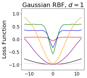
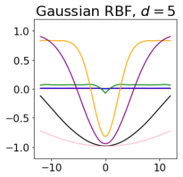
Refer to caption
Refer to caption
Refer to caption
Refer to caption
Refer to caption
Refer to caption
Refer to caption
Refer to caption
Refer to caption
Refer to caption
Refer to caption
Refer to caption
Refer to caption
Refer to caption
Refer to caption
Refer to caption
Figure 8: MMD Loss landscape for the Gaussian location model in dimensions d=1,5,25,100𝑑1525100d=1,5,25,100. The landscape is plotted for varying choices of kernels including a Gaussian RBF kernel, a MatΓ©rn kernel with smoothness 1212\frac{1}{2} or 3232\frac{3}{2} and an inverse-multiquadric kernel. For each kernel, we plot the loss function for varying values of the lengthscale parameter including l=0.1𝑙0.1l=0.1 (red), l=0.5𝑙0.5l=0.5 (blue), l=1𝑙1l=1 (green), l=5𝑙5l=5 (orange), l=10𝑙10l=10 (purple), l=25𝑙25l=25 (black) and l=50𝑙50l=50 (pink).
Refer to caption
Refer to caption
Refer to caption
Refer to caption
Refer to caption
Refer to caption
Refer to caption
Refer to caption
Refer to caption
Refer to caption
Refer to caption
Refer to caption
Refer to caption
Refer to caption
Refer to caption
Refer to caption
Figure 9: Gaussian distribution with unknown mean: Robustness as a function of the location of the Dirac for varying kernel and kernel lengthscales in dimensions d=1,5,25,100𝑑1525100d=1,5,25,100.
Refer to caption
Refer to caption
Refer to caption
Refer to caption
Refer to caption
Refer to caption
Refer to caption
Refer to caption
Refer to caption
Refer to caption
Refer to caption
Refer to caption
Refer to caption
Refer to caption
Refer to caption
Refer to caption
Figure 10: Gaussian distribution with unknown mean: Error in estimator as a function of the threshold Ο΅italic-Ο΅\epsilon for varying kernel and kernel lengthscales in dimensions d=1,5,25,100𝑑1525100d=1,5,25,100.
Refer to caption
Refer to caption
Figure 11: Gaussian location models - Performance of Sinkhorn Estimators in d=1𝑑1d=1 for varying values of the regularisation parameter Ο΅italic-Ο΅\epsilon. Left: l1subscript𝑙1l_{1} error as a function of the location of the Dirac. Right: l1subscript𝑙1l_{1} error as a function of the percentage of corrupted data points.

D.2 G-and-k Distribution

In order to implement MMD estimators, we will need to have access to derivatives of the generator, which are given as follows: βˆ‚Gθ​(u)/βˆ‚ΞΈ1=1subscriptπΊπœƒπ‘’subscriptπœƒ11\partial G_{\theta}(u)/\partial\theta_{1}=1 and

βˆ‚Gθ​(u)βˆ‚ΞΈ2subscriptπΊπœƒπ‘’subscriptπœƒ2\displaystyle\frac{\partial G_{\theta}(u)}{\partial\theta_{2}} =\displaystyle= (1+45​(1βˆ’exp(βˆ’ΞΈ3z(u))(1+exp(βˆ’ΞΈ3z(u)))​(1+z​(u)2)ΞΈ4​z​(u)\displaystyle\left(1+\frac{4}{5}\frac{\big{(}1-\exp(-\theta_{3}z(u)\big{)}}{\big{(}1+\exp(-\theta_{3}z(u)\big{)}}\right)\big{(}1+z(u)^{2}\big{)}^{\theta_{4}}z(u)
βˆ‚Gθ​(u)βˆ‚ΞΈ3subscriptπΊπœƒπ‘’subscriptπœƒ3\displaystyle\frac{\partial G_{\theta}(u)}{\partial\theta_{3}} =\displaystyle= 85​θ2​exp⁑(ΞΈ3​z​(u))(1+exp⁑(ΞΈ3​z​(u)))2​(1+z​(u)2)ΞΈ4​z​(u)285subscriptπœƒ2subscriptπœƒ3𝑧𝑒superscript1subscriptπœƒ3𝑧𝑒2superscript1𝑧superscript𝑒2subscriptπœƒ4𝑧superscript𝑒2\displaystyle\frac{8}{5}\;\theta_{2}\frac{\exp(\theta_{3}z(u))}{\big{(}1+\exp(\theta_{3}z(u))\big{)}^{2}}\big{(}1+z(u)^{2}\big{)}^{\theta_{4}}z(u)^{2}
βˆ‚Gθ​(u)βˆ‚ΞΈ4subscriptπΊπœƒπ‘’subscriptπœƒ4\displaystyle\frac{\partial G_{\theta}(u)}{\partial\theta_{4}} =\displaystyle= ΞΈ2​(1+0.8​(1βˆ’exp(βˆ’ΞΈ3z(u))(1+exp(βˆ’ΞΈ3z(u)))​(1+z​(u)2)ΞΈ4​log⁑(1+z​(u)2)​z​(u)\displaystyle\theta_{2}\left(1+0.8\frac{\big{(}1-\exp(-\theta_{3}z(u)\big{)}}{\big{(}1+\exp(-\theta_{3}z(u)\big{)}}\right)\big{(}1+z(u)^{2}\big{)}^{\theta_{4}}\log(1+z(u)^{2})z(u)

Note that these could also be obtained using automatic differentiation.
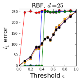
D.3 Stochastic Volatility Model

We can see the stochastic volatility model as a generative model with parameters ΞΈ=(ΞΈ1,ΞΈ2,ΞΈ3)πœƒsubscriptπœƒ1subscriptπœƒ2subscriptπœƒ3\theta=(\theta_{1},\theta_{2},\theta_{3}), which maps a sample u=(u0,u1,…,u2​T)𝑒subscript𝑒0subscript𝑒1…subscript𝑒2𝑇u=(u_{0},u_{1},\ldots,u_{2T}) which is 𝒩​(0,I2​TΓ—2​T)𝒩0subscript𝐼2𝑇2𝑇\mathcal{N}(0,I_{2T\times 2T}) distributed to a realisation y=(y1,…,yT)𝑦subscript𝑦1…subscript𝑦𝑇y=(y_{1},\ldots,y_{T}) of the stochastic volatility model. Here, Ο΅t=utsubscriptitalic-ϡ𝑑subscript𝑒𝑑\epsilon_{t}=u_{t} for tβ‰₯1𝑑1t\geq 1, h1=uT+1​σ2/(1βˆ’Ο•2)subscriptβ„Ž1subscript𝑒𝑇1superscript𝜎21superscriptitalic-Ο•2h_{1}=u_{T+1}\sqrt{\sigma^{2}/(1-\phi^{2})} and Ξ·t=σ​uT+tsubscriptπœ‚π‘‘πœŽsubscript𝑒𝑇𝑑\eta_{t}=\sigma u_{T+t} for all tβ‰₯2𝑑2t\geq 2. Note that it is possible to go back to the original parameterisation using Ο•=(exp⁑(ΞΈ1)βˆ’1)/(exp⁑(ΞΈ1)+1)italic-Ο•subscriptπœƒ11subscriptπœƒ11\phi=(\exp(\theta_{1})-1)/(\exp(\theta_{1})+1), ΞΊ=exp⁑(ΞΈ2)πœ…subscriptπœƒ2\kappa=\exp(\theta_{2}) and Οƒ=exp⁑(ΞΈ3/2)𝜎subscriptπœƒ32\sigma=\exp(\theta_{3}/2).
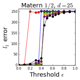
We can obtain the derivative process as follows: βˆ‚ΞΈ1yt=yt​(βˆ‚ΞΈ1ht)/2subscriptsubscriptπœƒ1subscript𝑦𝑑subscript𝑦𝑑subscriptsubscriptπœƒ1subscriptβ„Žπ‘‘2\partial_{\theta_{1}}y_{t}=y_{t}(\partial_{\theta_{1}}h_{t})/2, βˆ‚ΞΈ1h1=[(exp⁑(ΞΈ1/2)βˆ’exp⁑(βˆ’ΞΈ1/2))/(exp⁑(ΞΈ1/2)+exp⁑(βˆ’ΞΈ1/2))]​(h1/2)subscriptsubscriptπœƒ1subscriptβ„Ž1delimited-[]subscriptπœƒ12subscriptπœƒ12subscriptπœƒ12subscriptπœƒ12subscriptβ„Ž12\partial_{\theta_{1}}h_{1}=[(\exp(\theta_{1}/2)-\exp(-\theta_{1}/2))/(\exp(\theta_{1}/2)+\exp(-\theta_{1}/2))](h_{1}/2), βˆ‚ΞΈ1ht=(βˆ‚ΞΈ1Ο•)​htβˆ’1+ϕ​(βˆ‚ΞΈ1htβˆ’1)subscriptsubscriptπœƒ1subscriptβ„Žπ‘‘subscriptsubscriptπœƒ1italic-Ο•subscriptβ„Žπ‘‘1italic-Ο•subscriptsubscriptπœƒ1subscriptβ„Žπ‘‘1\partial_{\theta_{1}}h_{t}=(\partial_{\theta_{1}}\phi)h_{t-1}+\phi(\partial_{\theta_{1}}h_{t-1}) for t>1𝑑1t>1, βˆ‚ΞΈ1Ο•=2​exp⁑(ΞΈ1)/(exp⁑(ΞΈ1)+1)2subscriptsubscriptπœƒ1italic-Ο•2subscriptπœƒ1superscriptsubscriptπœƒ112\partial_{\theta_{1}}\phi=2\exp(\theta_{1})/(\exp(\theta_{1})+1)^{2}, βˆ‚ΞΈ2yt=ytsubscriptsubscriptπœƒ2subscript𝑦𝑑subscript𝑦𝑑\partial_{\theta_{2}}y_{t}=y_{t}, βˆ‚ΞΈ2ht=0subscriptsubscriptπœƒ2subscriptβ„Žπ‘‘0\partial_{\theta_{2}}h_{t}=0, βˆ‚ΞΈ3yt=yt​(βˆ‚ΞΈ3ht)/2subscriptsubscriptπœƒ3subscript𝑦𝑑subscript𝑦𝑑subscriptsubscriptπœƒ3subscriptβ„Žπ‘‘2\partial_{\theta_{3}}y_{t}=y_{t}(\partial_{\theta_{3}}h_{t})/2, βˆ‚ΞΈ3h1=h1/2subscriptsubscriptπœƒ3subscriptβ„Ž1subscriptβ„Ž12\partial_{\theta_{3}}h_{1}=h_{1}/2, βˆ‚ΞΈ3ht=ϕ​(βˆ‚ΞΈ3htβˆ’1)+(βˆ‚ΞΈ3Ξ·t)subscriptsubscriptπœƒ3subscriptβ„Žπ‘‘italic-Ο•subscriptsubscriptπœƒ3subscriptβ„Žπ‘‘1subscriptsubscriptπœƒ3subscriptπœ‚π‘‘\partial_{\theta_{3}}h_{t}=\phi(\partial_{\theta_{3}}h_{t-1})+(\partial_{\theta_{3}}\eta_{t}) for t>1𝑑1t>1 and βˆ‚ΞΈ3Ξ·t=Ξ·t/2subscriptsubscriptπœƒ3subscriptπœ‚π‘‘subscriptπœ‚π‘‘2\partial_{\theta_{3}}\eta_{t}=\eta_{t}/2.

Refer to caption
Refer to caption
Figure 12: Realisations from the stochastic volatility model. Left: 101010 realisations from the assumed model β„™ΞΈβˆ—subscriptβ„™superscriptπœƒ\mathbb{P}_{\theta^{*}} (i.e. stochastic volatility model with Gaussian noise). Right: Absolute value of these same realisations and 101010 realisations from the data generating process β„šβ„š\mathbb{Q} (i.e. stochastic volatility model with Cauchy noise).

D.4 Stochastic Lotka-Volterra Model

Besides simulating X1,tsubscript𝑋1𝑑X_{1,t} and X2,tsubscript𝑋2𝑑X_{2,t} we also required the coupled matrix diffusion process Jtsubscript𝐽𝑑J_{t} taking values in ℝ2Γ—2superscriptℝ22\mathbb{R}^{2\times 2} which satisfies the following SDE:

d​Jt𝑑subscript𝐽𝑑\displaystyle dJ_{t} =Jt​A​(X1,t,X2,t)​d​t+βˆ‘i=13Jt​Bi​(X1,t,X2,t)​d​Wi,t,absentsubscript𝐽𝑑𝐴subscript𝑋1𝑑subscript𝑋2𝑑𝑑𝑑superscriptsubscript𝑖13subscript𝐽𝑑subscript𝐡𝑖subscript𝑋1𝑑subscript𝑋2𝑑𝑑subscriptπ‘Šπ‘–π‘‘\displaystyle=J_{t}A(X_{1,t},X_{2,t})\,dt+\sum_{i=1}^{3}J_{t}B_{i}(X_{1,t},X_{2,t})dW_{i,t},

where

A​(x,y)𝐴π‘₯𝑦\displaystyle A(x,y) =(c1βˆ’c2​yc2​xc2​yc2​xβˆ’c3),B1​(x,y)=c12​(1x000),formulae-sequenceabsentsubscript𝑐1subscript𝑐2𝑦subscript𝑐2π‘₯subscript𝑐2𝑦subscript𝑐2π‘₯subscript𝑐3subscript𝐡1π‘₯𝑦subscript𝑐121π‘₯000\displaystyle=\left(\begin{array}[]{cc}c_{1}-c_{2}y&c_{2}x\\ c_{2}y&c_{2}x-c_{3}\end{array}\right),\qquad B_{1}(x,y)=\frac{\sqrt{c_{1}}}{2}\left(\begin{array}[]{cc}\frac{1}{\sqrt{x}}&0\\ 0&0\end{array}\right),
B2​(x,y)subscript𝐡2π‘₯𝑦\displaystyle B_{2}(x,y) =c22​(βˆ’yxβˆ’xyyxxy),B3​(x,y)=c32​(000βˆ’1x),formulae-sequenceabsentsubscript𝑐22𝑦π‘₯π‘₯𝑦𝑦π‘₯π‘₯𝑦subscript𝐡3π‘₯𝑦subscript𝑐320001π‘₯\displaystyle=\frac{\sqrt{c_{2}}}{2}\left(\begin{array}[]{cc}-\sqrt{\frac{y}{x}}&-\sqrt{\frac{x}{y}}\\ \sqrt{\frac{y}{x}}&\sqrt{\frac{x}{y}}\end{array}\right),\qquad B_{3}(x,y)=\frac{\sqrt{c_{3}}}{2}\left(\begin{array}[]{cc}0&0\\ 0&-\frac{1}{\sqrt{x}}\end{array}\right),

and subject to the initial condition J0=I2Γ—2subscript𝐽0subscript𝐼22J_{0}=I_{2\times 2}.