Embedding Biomedical Ontologies by Jointly Encoding
Network Structure and Textual Node Descriptors

Abstract

Network Embedding (ne) methods, which map network nodes to low-dimensional feature vectors, have wide applications in network analysis and bioinformatics. Many existing ne methods rely only on network structure, overlooking other information associated with the nodes, e.g., text describing the nodes. Recent attempts to combine the two sources of information only consider local network structure. We extend node2vec, a well-known ne method that considers broader network structure, to also consider textual node descriptors using recurrent neural encoders. Our method is evaluated on link prediction in two networks derived from umls. Experimental results demonstrate the effectiveness of the proposed approach compared to previous work.

1 Introduction

Network Embedding (ne) methods map each node of a network to an embedding, meaning a low-dimensional feature vector. They are highly effective in network analysis tasks involving predictions over nodes and edges, for example link prediction Lu and Zhou (2010), and node classification Sen et al. (2008).

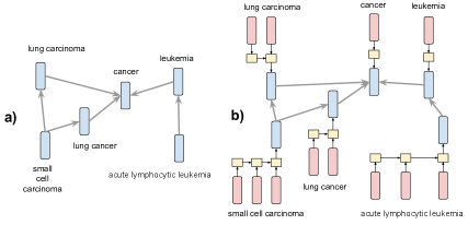
Figure 1: Example network with nodes associated with textual descriptors. a) A model where each node is represented by a vector (node embedding) from a look-up table. b) A model where each node embedding is generated compositionally from the word embeddings of its descriptor via an rnn. The latter model can learn node embeddings from both the network structure and the word sequences of the textual descriptors.

Early ne methods, such as deepwalk Perozzi et al. (2014), line Tang et al. (2015), node2vec Grover and Leskovec (2016), gcns Kipf and Welling (2016), leverage information from the network structure to produce embeddings that can reconstruct node neighborhoods. The main advantage of these structure-oriented methods is that they encode the network context of the nodes, which can be very informative. The downside is that they typically treat each node as an atomic unit, directly mapped to an embedding in a look-up table (Fig. 1a). There is no attempt to model information other than the network structure, such as textual descriptors (labels) or other meta-data associated with the nodes.

More recent ne methods, e.g., cane Tu et al. (2017), wane Shen et al. (2018), produce embeddings by combining the network structure and the text associated with the nodes. These content-oriented methods embed networks whose nodes are rich textual objects (often whole documents). They aim to capture the compositionality and semantic similarities in the text, encoding them with deep learning methods. This approach is illustrated in Fig. 1b. However, previous methods of this kind considered impoverished network contexts when embedding nodes, usually single-edge hops, as opposed to the non-local structure considered by most structure-oriented methods.

When embedding biomedical ontologies, it is important to exploit both wider network contexts and textual node descriptors. The benefit of the latter is evident, for example, in ‘acute leukemia’ is-a ‘leukemia’. To be able to predict (or reconstruct) this is-a relation from the embeddings of ‘acute leukemia’ and ‘leukemia’ (and the word embeddings of their textual descriptors in Fig. 1b), a ne method only needs to model the role of ‘acute’ as a modifier that can be included in the descriptor of a node (e.g., a disease node) to specify a sub-type. This property can be learned (and encoded in the word embedding of ‘acute’) if several similar is-a edges, with ‘acute’ being the only extra word in the descriptor of the sub-type, exist in the network. This strategy would not however be successful in ‘p53’ (a protein) is-a ‘tumor suppressor’, where no word in the descriptors frequently denotes sub-typing. Instead, by considering the broader network context of the nodes (i.e. longer paths that connect them), a ne method can detect that the two nodes have common neighbors and, hence, adjust the two node embeddings (and the word embeddings of their descriptors) to be close in the representation space, making it more likely to predict an is-a relation between them.

We propose a new ne method that leverages the strengths of both structure and content-oriented approaches. To exploit wide network contexts, we follow node2vec Grover and Leskovec (2016) and generate random walks to construct the network neighborhood of each node. The skipgram model Mikolov et al. (2013) is then used to learn node embeddings that successfully predict the nodes in each walk, from the node at the beginning of the walk. To enrich the node embeddings with information from their textual descriptors, we replace the node2vec look-up table with various architectures that operate on the word embeddings of the descriptors. These include simply averaging the word embeddings of a descriptor, and applying recurrent deep learning encoders. The proposed method can be seen as an extension of node2vec that incorporates textual node descriptors. We evaluate several variants of the proposed method on link prediction, a standard evaluation task for ne methods. We use two biomedical networks extracted from umls Bodenreider (2004), with part-of and is-a relations, respectively. Our method outperforms several existing structure and content-oriented methods on both datasets. We make our datasets and source code available.

2 Related work

Network Embedding (ne) methods, a type of representation learning, are highly effective in network analysis tasks involving predictions over nodes and edges. Link prediction has been extensively studied in social networks Wang et al. (2015), and is particularly relevant to bioinformatics where it can help, for example, to discover interactions between proteins, diseases, and genes Lei and Ruan (2013); Shojaie (2013); Grover and Leskovec (2016). Node classification can also help analyze large networks by automatically assigning roles or labels to nodes Ahmed et al. (2018); Sen et al. (2008). In bioinformatics, this approach has been used to identify proteins whose mutations are linked with particular diseases Agrawal et al. (2018).

A typical structure-oriented ne method is deepwalk Perozzi et al. (2014), which learns node embeddings by applying word2vec’s skipgram model Mikolov et al. (2013) to node sequences generated via random walks on the network. node2vec Grover and Leskovec (2016) explores different strategies to perform random walks, introducing hyper-parameters to guide them and generate more flexible neighborhoods. line Tang et al. (2015) learns node embeddings by exploiting first- and second-order proximity information in the network.  Wang et al. (2016) learn node embeddings that preserve the proximity between 2-hop neighbors using a deep autoencoder. Yu et al. (2018) encode node sequences generated via random walks, by mapping the walks to low dimensional embeddings, through an lstm autoencoder. To avoid overfitting, they use a generative adversarial training process as regularization. Graph Convolutional Networks (gcns) are a graph encoding framework that also falls within this paradigm Kipf and Welling (2016); Schlichtkrull et al. (2018). Unlike other methods that use random walks or static neighbourhoods, gcns use iterative neighbourhood averaging strategies to account for non-local graph structure. All the aforementioned methods only encode the structural information into node embeddings, ignoring textual or other information that can be associated with the nodes of the network.

Previous work on biomedical ontologies (e.g., Gene Ontology, go) suggested that their terms, which are represented through textual descriptors, have compositional structure. By modeling it, we can create richer representations of the data encoded in the ontologies Mungall (2004); Ogren et al. (2003, 2004). Ogren et al. (2003) strengthen the argument of compositionality by observing that many go terms contain other go terms. Also, they argue that substrings that are not go terms appear frequently and often indicate semantic relationships. Ogren et al. (2004) use finite state automata to represent go terms and demonstrate how small conceptual changes can create biologically meaningful candidate terms.

In other work on ne methods, cene Sun et al. (2016) treats textual descriptors as a special kind of node, and uses bidirectional recurrent neural networks (rnns) to encode them. cane Tu et al. (2017) learns two embeddings per node, a text-based one and an embedding based on network structure. The text-based one changes when interacting with different neighbors, using a mutual attention mechanism. wane Shen et al. (2018) also uses two types of node embeddings, text-based and structure-based. For the text-based embeddings, it matches important words across the textual descriptors of different nodes, and aggregates the resulting alignment features. In spite of performance improvements over structure-oriented approaches, these content-aware methods do not thoroughly explore the network structure, since they consider only direct neighbors.

By contrast, we utilize node2vec to obtain wider network neighborhoods via random walks, a typical approach of structure-oriented methods, but we also use rnns to encode the textual descriptors, as in some content-oriented approaches. Unlike cene, however, we do not treat texts as separate nodes; unlike cane, we do not learn separate embeddings from texts and network structure; and unlike wane, we do not align the descriptors of different nodes. We generate the embedding of each node from the word embeddings of its descriptor via the rnn (Fig. 1), but the parameters of the rnn, the word embeddings, hence also the node embeddings are updated during training to predict node2vec’s neighborhoods.

Although we use node2vec to incorporate network context in the node embeddings, other neighborhood embedding methods, such as gcns, could easily be used too. Similarly, text encoders other than rnns could be applied. For example, Mishra et al. (2019) try to detect abusive language in tweets with a semi-supervised learning approach based on gcns. They exploit the network structure and also the labels associated with the tweets, taking into account the linguistic behavior of the authors.

3 Proposed Node Embedding Approach

Consider a network (graph) $G=\left<V,E,S\right>$, where $V$ is the set of nodes (vertices); $E\subseteq V\times V$ is the set of edges (links) between nodes; and $S$ is a function that maps each node $v\in V$ to its textual descriptor $S(v)=\left<w_{1},w_{2},\ldots,w_{n}\right>$, where $n$ is the word length of the descriptor, and each word $w_{i}$ comes from a vocabulary $W$. We consider only undirected, unweighted networks, where all edges represent instances of the same (single) relationship (e.g., is-a or part-of). Our approach, however, can be extended to directed weighted networks with multiple relationship types. We learn an embedding $f(v)\in\mathbb{R}^{d}$ for each node $v\in V$. As a side effect, we also learn a word embedding $e(w)$ for each vocabulary word $w\in W$.

To incorporate structural information into the node embeddings, we maximize the predicted probabilities $p(u|v)$ of observing the actual neighbors $u\in N(v)$ of each ‘focus’ node $v\in V$, where $N(v)$ is the neighborhood of $v$, and $p(u|v)$ is predicted from the node embeddings of $u$ and $v$. The neighbors $N(v)$ of $v$ are not necessarily directly connected to $v$. In real-world networks, especially biomedical, many nodes have few direct neighbors. We use node2vec Grover and Leskovec (2016) to obtain a larger neighborhood for each node $v$, by generating random walks from $v$. For every focus node $v\in V$, we compute $r$ random walks (paths) $P_{v,i}=\left<v_{i,1}=v,v_{i,2},...,v_{i,k}\right>$ ($i=1,\dots,r$) of fixed length $k$ through the network ($v_{i,j}\in V$). The predicted probability $p(v_{i,j}=u)$ of observing node $u$ at step $j$ of a walk $P_{v,i}$ that starts at focus node $v$ is taken to depend only on the embeddings of $u,v$, i.e., $p(v_{i,j}=u)=p(u|v)$, and can be estimated with a softmax as in the skipgram model Mikolov et al. (2013):

$$p(u|v)=\dfrac{\exp(f^{\prime}(u)\cdot f(v))}{\sum_{u^{\prime}\in V}\exp(f^{\prime}(u^{\prime})\cdot f(v))}$$ (1)

where it is assumed that each node $v$ has two different node embeddings, $f(v),f^{\prime}(v)$, used when $v$ is the focus node or the predicted neighbor, respectively, and $\cdot$ denotes the dot product. node2vec minimizes the following objective function:

$$L=-\sum_{v\in V}\sum_{i=1}^{r}\sum_{j=2}^{k}\log p(v_{i,j}|v_{i,1}=v)$$ (2)

in effect maximizing the likelihood of observing the actual neighbors $v_{i,j}$ of each focus node $v$ that are encountered during the $r$ walks $P_{v,i}=\left<v_{i,1}=v,v_{i,2},...,v_{i,k}\right>$ ($i=1,\dots,r$) from $v$. Calculating $p(u|v)$ using a softmax (Eq. 1) is computationally inefficient. We apply negative sampling instead, as in word2vec Mikolov et al. (2013). Thus, node2vec is analogous to skipgram word2vec, but using random walks from each focus node, instead of using a context window around each focus word in a corpus.

As already mentioned, the original node2vec does not consider the textual descriptors of the nodes. It treats each node embedding $f(v)$ as a vector representing an atomic unit, the node $v$; a look-up table directly maps each node $v$ to its embedding $f(v)$. This does not take advantage of the flexibility and richness of natural language (e.g., synonyms, paraphrases), nor of its compositional nature. To address this limitation, we substitute the look-up table where node2vec stores the embedding $f(v)$ of each node $v$ with a neural sequence encoder that produces $f(v)$ from the word embeddings of the descriptor $S(v)$ of $v$.

More formally, let every word $w\in W$ have two embeddings ${e(w)}$ and ${e^{\prime}(w)}$, used when $w$ occurs in the descriptor of a focus node, and when $w$ occurs in the descriptor of a neighbor of a focus node (in a random walk), respectively. For every node $v\in V$ with descriptor $S(v)=(w_{1},\ldots,w_{n})$, we create the sequences $T(v)=\left<{e(w_{1})},\ldots,{e(w_{n})}\right>$ and $T^{\prime}(v)=\left<{e^{\prime}(w_{1})},\ldots,{e^{\prime}(w_{n})}\right>$. We then set $f(v)=\mathrm{\textsc{enc}}(T(v))$ and $f^{\prime}(v)=\mathrm{\textsc{enc}}(T^{\prime}(v))$, where enc is the sequence encoder. We outline below three specific possibilities for enc, though it can be any neural text encoder. Note that the embeddings $f(v)$ and $f^{\prime}(v)$ of each node $v$ are constructed from the word embeddings $T(v)$ and $T^{\prime}(v)$, respectively, of its descriptor $S(v)$ by the encoder enc. The word embeddings of the descriptor and the parameters of enc, however, are also optimized during back-propagation, so that the resulting node embeddings will predict (Eq. 1) the actual neighbors of each focus node (Fig. 2). For simplicity, we only mention $f(v)$ and $T(v)$ below, but the same applies to $f^{\prime}(v)$ and $T^{\prime}(v)$.

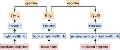
Figure 2: Illustration of the proposed ne approach.

avg-n2v: For every node $v\in V$, this model constructs the node’s embedding $f(v)$ by simply averaging the word embeddings $T(v)=\left<{e(w_{1})},\ldots,{e(w_{n})}\right>$ of $S(v)=(w_{1},w_{2},\ldots,w_{n})$.

$$f(v)=\dfrac{1}{n}\sum_{i=1}^{n}{e(w_{i})}$$ (3)

gru-n2v: Although averaging word embeddings is effective in text categorization Joulin et al. (2016), it ignores word order. To account for order, we apply rnns with gru cells Cho et al. (2014) instead. For each node $v\in V$ with descriptor $S(v)=\left<w_{1},\dots,w_{n}\right>$, this method computes $n$ hidden state vectors $H=\left<h_{1},\dots,h_{n}\right>={\mathrm{\textsc{gru}}}({e(w_{1})},\dots,{e(w_{n})})$. The last hidden state vector $h_{n}$ is the node embedding $f(v)$.

bigru-max-res-n2v: This method uses a bidirectional rnn Schuster and Paliwal (1997). For each node $v$ with descriptor $S(v)=\left<w_{1},w_{2},\ldots,w_{n}\right>$, a bidirectional gru (bigru) computes two sets of $n$ hidden state vectors, one for each direction. These two sets are then added to form the output $H$ of the bigru:

$${H_{f}} = {\mathrm{\textsc{gru}}_{f}}({e(w_{1})},\dots,{e(w_{n})})$$ (4)

$${H_{b}} = {\mathrm{\textsc{gru}}_{b}}({e(w_{1})},\dots,{e(w_{n})})$$ (5)

$$H = {H_{f}}+{H_{b}}$$ (6)

where _f, _b denote the forward and backward directions, and $+$ indicates component-wise addition. We add residual connections He et al. (2015) from each word embedding ${e(w_{t})}$ to the corresponding hidden state $h_{t}$ of $H$. Instead of using the final forward and backward states of $H$, we apply max-pooling Collobert and Weston (2008); Conneau et al. (2017) over the state vectors $h_{t}$ of $H$. The output of the max pooling is the node embedding $f(v)$. Figure 3 illustrates this method.

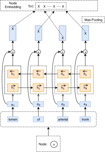
Figure 3: Obtaining the embedding of a node $v$ by applying a bigru encoder with max-pooling and residuals to the embeddings of $v$’s textual descriptor.

Additional experiments were conducted with several variants of the last encoder. A unidirectional gru instead of a bigru, and a bigru with self-attention Bahdanau et al. (2015) instead of max-pooling were also tried. To save space, we described only the best performing variant.

4 Experiments

We investigate the effectiveness of our proposed approach by conducting link prediction experiments on two biomedical datasets derived from umls. Furthermore, we devise a new approach of generating negative edges for the link prediction evaluation – beyond just random negatives – that makes the problem more difficult and aligns more with real-world use-cases. We also conduct a qualitative analysis, showing that the proposed framework does indeed leverage both the textual descriptors and the network structure.

4.1 Datasets

We created our datasets from the umls ontology, which contains approx. 3.8 million biomedical concepts and 54 semantic relationships. The relationships become edges in the networks, and the concepts become nodes. Each concept (node) is associated with a textual descriptor. We extract two types of semantic relationships, creating two networks. The first, and smaller one, consists of part-of relationships where each node represents a part of the human body. The second network contains is-a relationships, and the concepts represented by the nodes vary across the spectrum of biomedical entities (diseases, proteins, genes, etc.). To our knowledge, the is-a network is one of the largest datasets employed for link prediction and learning network embeddings. Statistics for the two datasets are shown in Table 1.

Statistics	is-a	part-of
Nodes	294,693	16,894
Edges	356,541	19,436
Training true positive edges	294,692	16,893
Training true negative edges	294,692	16,893
Test true positive edges	61,849	2,543
Test true negative edges	61,849	2,543
Avg. descriptor length	5 words	6 words
Max. descriptor length	31 words	14 words

Table 1: Statistics of the two datasets (is-a, part-of). The true positive and true negative edges are used in the link prediction experiments.

4.2 Baseline Node Embedding Methods

We compare our proposed methods to baselines of two types: structure-oriented methods, which solely focus on network structure, and content-oriented methods that try to combine the network structure with the textual descriptors of the nodes (albeit using impoverished network neighborhoods so far). For the first type of methods, we employ node2vec Grover and Leskovec (2016), which uses a biased random walk algorithm based on deepwalk Perozzi et al. (2014) to explore the structure of the network more efficiently. Our work can be seen as an extension of node2vec that incorporates textual node descriptors, as already discussed, hence it is natural to compare to node2vec. As a content-oriented baseline we use cane Tu et al. (2017), which learns separate text-based and network-based embeddings, and uses a mutual attention mechanism to dynamically change the text-based embeddings for different neighbors (Section 2). cane only considers the direct neighbors of each node, unlike node2vec, which considers larger neighborhoods obtained via random walks.

4.3 Link Prediction

In link prediction, we are given a network with a certain fraction of edges removed. We need to infer these missing edges by observing the incomplete network, facilitating the discovery of links (e.g., unobserved protein-protein interactions).

Concretely, given a network we first randomly remove some percentage of edges, ensuring that the network remains connected so that we can perform random walks over it. Each removed edge $e$ connecting nodes $v_{1},v_{2}$ is treated as a true positive, in the sense that a link prediction method should infer that an edge should be added between $v_{1},v_{2}$. We also use an equal number of true negatives, which are pairs of nodes $v^{\prime}_{1},v^{\prime}_{2}$ with no edge between $v^{\prime}_{1},v^{\prime}_{2}$ in the original network. When evaluating ne methods, a link predictor is given true positive and true negative pairs of nodes, and is required to discriminate between the two classes by examining only the node embeddings of each pair. Node embeddings are obtained by applying a ne method to the pruned network, i.e., after removing the true positives. A ne method is considered better than another one, if it leads to better performance of the same link predictor.

We experiment with two approaches to obtain true negatives. In Random Negative Sampling, we randomly select pairs of nodes that were not directly connected (by a single edge) in the original network. In Close Proximity Negative Sampling, we iterate over the nodes of the original network considering each one as a focus. For each focus node $v$, we want to find another node $u$ in close proximity that is not an ancestor or descendent (e.g., parent, grandparent, child, grandchild) of $v$ in the is-a or part-of hierarchy, depending on the dataset. We want $u$ to be close to $v$, to make it more difficult for the link predictor to infer that $u$ and $v$ should not be linked. We do not, however, want $u$ to be an ancestor or descendent of $v$, because the is-a and part-of relationships of our datasets are transitive. For example, if $u$ is a grandparent of $v$, it could be argued that inferring that $u$ and $v$ should be linked, is not an error. To satisfy these constraints, we first find the ancestors of $v$ that are between 2 to 5 hops away from $v$ in the original network. We randomly select one of these ancestors, and then we randomly select as $u$ one of the ancestor’s children in the original network, ensuring that $u$ was not an ancestor or descendent of $v$ in the original network. In both approaches, we randomly select as many true negatives as the true positives, discarding the remaining true negatives.

We experimented with two link predictors:

Cosine similarity link predictor (cs): Given a pair of nodes $v_{1},v_{2}$ (true positive or true negative edge), cs computes the cosine similarity (ignoring negative scores) between the two node embeddings as $s(v_{1},v_{2})=\max(0,\cos(f(v_{1}),f(v_{2})))$, and predicts an edge between the two nodes if $s(v_{1},v_{2})\geq t$, where $t$ is a threshold. We evaluate the predictor on the true positives and true negatives (shown as ‘test’ true positives and ‘test’ true negatives in Table 1) by computing auc (area under roc curve), in effect considering the precision and recall of the predictor for varying $t$.

Logistic regression link predictor (lr): Given a pair of nodes $v_{1},v_{2}$, lr computes the Hadamard (element-wise) product of the two node embeddings $f(v_{1})\odot f(v_{2})$ and feeds it to a logistic regression classifier to obtain a probability estimate $p$ that the two nodes should be linked. The predictor predicts an edge between $v_{1},v_{2}$ if $p\geq t$. We compute auc on a test set by varying $t$. The test set of this predictor is the same set of true positives and true negatives (with Random or Close Proximity Negative Sampling) that we use when evaluating the cs predictor. The training set of the logistic regression classifier contains as true positives all the other edges of the network that remain after the true positives of the test set have been removed, and an equal number of true negatives (with the same negative sampling method as in the test set) that are not used in the test set.

4.4 Implementation Details

For node2vec and our ne methods, which can be viewed as extensions of node2vec, the dimensionality of the node embeddings is 30. The dimensionality of the word embeddings (in our ne methods) is also 30. In the random walks, we set $r$ = 5, $l$ = 40, $k$ = 10 for is-a, and $r$ = 10, $l$ = 40, $k$ = 10 for part-of; these hyper-parameters were not particularly tuned, and their values were selected mostly to speed up the experiments. We train for one epoch with a batch size of 128, setting the number of skipgram’s negative samples to 2. We use the Adam Kingma and Ba (2015) optimizer in our ne methods. We implemented our ne methods and the two link predictors using PyTorch Paszke et al. (2017) and Scikit-Learn Pedregosa et al. (2011). For node2vec and cane, we used the implementations provided.

For cane, we set the dimensionality of the node embeddings to 200, as in the work of Tu et al. (2017). We also tried 30-dimensional node embeddings, as in node2vec and our ne methods, but performance deteriorated significantly.

4.5 Link Prediction Results

Link prediction results for the is-a and part-of networks are reported in Tables 2 and 3. All content-oriented ne methods (cane and our extensions of node2vec) clearly outperform the structure-oriented method (node2vec) on both datasets in both negative edge sampling settings, showing that modeling the textual descriptors of the nodes is critical. Furthermore, all methods perform much worse with Close Proximity Negative Sampling, confirming that the latter produces more difficult link prediction datasets.

All of our ne methods (content-aware extensions of node2vec) outperform node2vec and cane in every case, especially with Close Proximity Negative Sampling. We conclude that it is important to model not just the textual descriptor of a node or its direct neighbors, but as much non-local network structure as possible.

	Random	Close
	Negative	Proximity
NE Method + Link Predictor	Sampling	Sampling
Node2Vec + CS	66.6	54.3
CANE + CS	94.1	69.6
Avg-N2V + CS	95.0	78.6
GRU-N2V + CS	98.7	79.2
BiGRU-Max-Res-N2V + CS	98.5	79.0
Node2Vec + LR CANE + LR Avg-N2V + LR GRU-N2V + LR BiGRU-Max-Res-N2V + LR	77.2 95.3 97.6 99.0 99.3	56.3 70.0 73.9 79.6 82.1

Table 2: auc scores (%) for the is-a dataset. Best scores per link predictor (cs, lr) shown in bold.

	Random	Close
	Negative	Proximity
NE Method + Link Predictor	Sampling	Sampling
Node2Vec + CS	76.8	61.8
CANE + CS	93.9	75.3
Avg-N2V + CS	95.9	81.8
GRU-N2V + CS	98.0	83.1
BiGRU-Max-Res-N2V + CS	98.5	83.3
Node2Vec + LR CANE + LR Avg-N2V + LR GRU-N2V + LR BiGRU-Max-Res-N2V + LR	85.2 94.4 97.6 99.0 99.5	66.5 76.3 79.4 85.6 88.6

Table 3: auc scores (%) for the part-of dataset. Best scores per link predictor (cs, lr) shown in bold.

For part-of relations (Table 3), bigru-max-res-n2v obtains the best results with both link predictors (cs, lr) in both negative sampling settings, but the differences from gru-n2v are very small in most cases. For is-a (Table 2), bigru-max-res-n2v obtains the best results with the lr predictor, and only slightly inferior results than gru-n2v with the cs predictor. The differences of these two ne methods from avg-n2v are larger, indicating that recurrent neural encoders of textual descriptors are more effective than simply averaging the word embeddings of the descriptors.

Finally, we observe that the best results of the lr predictor are better than those of the cs predictor, in both datasets and with both negative edge sampling approaches, with the differences being larger with Close Proximity Sampling. This is as one would expect, because the logistic regression classifier can assign different weights to the dimensions of the node embeddings, depending on their predictive power, whereas cosine similarity assigns the same importance to all dimensions.

Target Node: Left Eyeball (part-of)
Most Similar Embeddings	Cos	Hops
equator of left eyeball	99.3	1
episcleral layer of left eyeball	99.2	4
cavity of left eyeball	99.1	1
wall of left eyeball	99.0	1
vascular layer of left eyeball	98.9	1

Target Node: Lung Carcinoma (is-a)
Most Similar Embeddings	Cos	Hops
recurrent lung carcinoma	97.6	1
papillary carcinoma	97.1	2
lung pleomorphic carcinoma	97.0	3
ureter carcinoma	96.6	2
lymphoepithelioma-like lung carcinoma	96.6	3

Table 4: Examples of nodes whose embeddings are closest (cosine similarity, Cos) to the embedding of a target node in the part-of (top) and is-a (bottom) datasets. We also show the distances (number of edges, Hops) between the nodes in the networks.

4.6 Qualitative Analysis

To better understand the benefits of leveraging both network structure and textual descriptors, we present examples from the two datasets.

Most similar embeddings: Table 4 presents the five nearest nodes for two target nodes (‘Left Eyeball’ and ‘Lung Carcinoma’), based on the cosine similarity of the corresponding node embeddings in the part-of and is-a networks, respectively. We observe that all nodes in the part-of example are very similar content-wise to our target node. Furthermore, the model captures the semantic relationship between concepts, since most of the returned nodes are actually parts of ‘Left Eyeball’. The same pattern is observed in the is-a example, with the exception of ‘ureter carcinoma’, which is not directly related with ‘lung carcinoma’, but is still a form of cancer. Finally, it is clear that the model extracts meaningful information from both the textual content of each node and the network structure, since the returned nodes are closely located in the network (Hops 1–4).

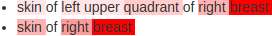
(a) Two nodes connected by a part-of edge.

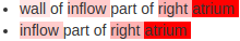
(b) Two nodes connected by a part-of edge.

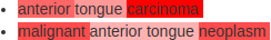
(c) Two nodes connected by an is-a edge.

Figure 4: Visualization of the importance that bigru-max-res-n2v assigns to the words of the descriptors of the nodes of three edges. Edges (a) and (b) are from the part-of dataset. Edge (c) is from the is-a dataset.

Edges/Descriptors	BN2V	CANE	N2V	Hops
(a) bariatric surgery (b) bypass gastrojejunostomy	82.7	38.0	56.2	11
(a) anatomical line (b) anterior malleolar fold	82.3	29.0	50.0	22
(a) zone of biceps brachii (b) short head of biceps brachii	93.0	70.0	61.6	13

Table 5: Examples of true positive edges, showing how structure and textual descriptors affect node embeddings. The first two edges are is-a, the third one is part-of. The ne methods used are bigru-max-res-n2v (bn2v), cane and node2vec (n2v). We report cosine similarities between node embeddings and the distances between the nodes (number of edges, Hops) in the networks after removing true positive edges.

Heatmap visualization: bigru-max-res-n2v can be extended to highlight the words in each textual descriptor that mostly influence the corresponding node embedding. Recall that this ne method applies a max-pooling operator (Fig. 3) over the state vectors $h_{1},\dots,h_{n}$ of the words $w_{1},\dots,w_{n}$ of the descriptor, keeping the maximum value per dimension across the state vectors. We count how many dimension-values the max-pooling operator keeps from each state vector $h_{i}$, and we treat that count (normalized to $[0,1]$) as the importance score of the corresponding word $w_{i}$. We then visualize the importance scores as heatmaps of the descriptors. In the first two example edges of Fig. 4, the highest importance scores are assigned to words indicating body parts, which is appropriate given that the edges indicate part-of relations. In the third example edge, the highest importance score of the first descriptor is assigned to ‘carcinoma’, and the highest importance scores of the second descriptor are shared by ‘malignant’ and ‘neoplasm’; again, this is appropriate, since these words indicate an is-a relation.

Case Study: In Table 5, we present examples that illustrate learning from both the network structure and textual descriptors. All three edges are true positives, i.e., they were initially present in the network and they were removed to test link prediction. In the first two edges, which come from the is-a network, the node descriptors share no words. Nevertheless, bigru-max-res-n2v (bn2v) produces node embeddings with high cosine similarities, much higher than node2vec that uses only network structure, presumably because the word embeddings (and neural encoder) of bn2v correctly capture lexical relations (e.g., near-synonyms). Although cane also considers the textual descriptors, its similarity scores are much lower, presumably because it uses only local neighborhoods (single-edge hops). The nodes in the third example, which come from the part-of network, have a larger word overlap. node2vec is unaware of this overlap and produces the lowest score. The two content-oriented methods (bn2v, cane) produce higher scores, but again bn2v produces a much higher similarity, presumably because it uses larger neighborhoods. In all three edges, the two nodes are distant ($>$10 hops), yet bn2v produces high similarity scores.

5 Conclusions and Future Work

We proposed a new method to learn content-aware node embeddings, which extends node2vec by considering the textual descriptors of the nodes. The proposed approach leverages the strengths of both structure- and content-oriented node embedding methods. It exploits non-local network neighborhoods generated by random walks, as in the original node2vec, and allows integrating various neural encoders of the textual descriptors. We evaluated our models on two biomedical networks extracted from umls, which consist of part-of and is-a edges. Experimental results with two link predictors, cosine similarity and logistic regression, demonstrated that our approach is effective and outperforms previous methods which rely on structure alone, or model content along with local network context only.

In future work, we plan to experiment with networks extracted from other biomedical ontologies and knowledge bases. We also plan to explore if the word embeddings that our methods generate can improve biomedical question answering systems McDonald et al. (2018).

Appendix

Appendix A CANE Hyper-parameters

cane has 3 hyper-parameters, denoted $\alpha$, $\beta$, $\gamma$, which control to what extent it uses information from network structure or textual descriptors. We learned these hyper-parameters by employing the HyperOpt Bergstra et al. (2013) on the validation set. All three hyper-parameters had the same search space: $[0.2,1,0]$ with a step of $0.1$. The optimization ran for 30 trials for both datasets. Table 6 reports the resulting hyper-parameter values.

Parameters	part-of	is-a
$\alpha$	0.2	0.7
$\beta$	1.0	0.7
$\gamma$	1.0	0.7

Table 6: Hyper-parameter values used in cane.

References

- Agrawal et al. (2018) Monica Agrawal, Marinka Zitnik, and Jure Leskovec. 2018. Large-scale analysis of disease pathways in the human interactome. Pacific Symposium on Biocomputing. Pacific Symposium on Biocomputing, 23:111–122.
- Ahmed et al. (2018) Nesreen K. Ahmed, Ryan A. Rossi, John Boaz Lee, Xiangnan Kong, Theodore L. Willke, Rong Zhou, and Hoda Eldardiry. 2018. Learning role-based graph embeddings. CoRR, abs/1802.02896.
- Bahdanau et al. (2015) Dzmitry Bahdanau, Kyunghyun Cho, and Yoshua Bengio. 2015. Neural machine translation by jointly learning to align and translate. In 3rd International Conference on Learning Representations, ICLR 2015, San Diego, CA, USA, May 7-9, 2015, Conference Track Proceedings.
- Bergstra et al. (2013) James Bergstra, Daniel L K Yamins, and David D. Cox. 2013. Hyperopt: A python library for optimizing the hyperparameters of machine learning algorithms.
- Bodenreider (2004) Olivier Bodenreider. 2004. The unified medical language system (UMLS): integrating biomedical terminology. Nucleic Acids Research, 32(Database-Issue):267–270.
- Cho et al. (2014) Kyunghyun Cho, Bart van Merrienboer, Çaglar Gülçehre, Dzmitry Bahdanau, Fethi Bougares, Holger Schwenk, and Yoshua Bengio. 2014. Learning phrase representations using RNN encoder-decoder for statistical machine translation. In Proceedings of the 2014 Conference on Empirical Methods in Natural Language Processing, EMNLP 2014, October 25-29, 2014, Doha, Qatar, A meeting of SIGDAT, a Special Interest Group of the ACL, pages 1724–1734.
- Collobert and Weston (2008) Ronan Collobert and Jason Weston. 2008. A unified architecture for natural language processing: deep neural networks with multitask learning. In Machine Learning, Proceedings of the Twenty-Fifth International Conference (ICML 2008), Helsinki, Finland, June 5-9, 2008, pages 160–167.
- Conneau et al. (2017) Alexis Conneau, Douwe Kiela, Holger Schwenk, Loïc Barrault, and Antoine Bordes. 2017. Supervised learning of universal sentence representations from natural language inference data. In Proceedings of the 2017 Conference on Empirical Methods in Natural Language Processing, EMNLP 2017, Copenhagen, Denmark, September 9-11, 2017, pages 670–680.
- Grover and Leskovec (2016) Aditya Grover and Jure Leskovec. 2016. node2vec: Scalable feature learning for networks. In KDD, pages 855–864. ACM.
- He et al. (2015) Kaiming He, Xiangyu Zhang, Shaoqing Ren, and Jian Sun. 2015. Deep residual learning for image recognition. CoRR, abs/1512.03385.
- Joulin et al. (2016) Armand Joulin, Edouard Grave, Piotr Bojanowski, and Tomas Mikolov. 2016. Bag of tricks for efficient text classification. CoRR, abs/1607.01759.
- Kingma and Ba (2015) Diederik P. Kingma and Jimmy Ba. 2015. Adam: A method for stochastic optimization. CoRR, abs/1412.6980.
- Kipf and Welling (2016) Thomas N. Kipf and Max Welling. 2016. Semi-supervised classification with graph convolutional networks. CoRR, abs/1609.02907.
- Lei and Ruan (2013) Chengwei Lei and Jianhua Ruan. 2013. A novel link prediction algorithm for reconstructing protein-protein interaction networks by topological similarity. Bioinformatics, 29(3):355–364.
- Lu and Zhou (2010) Linyuan Lu and Tao Zhou. 2010. Link prediction in complex networks: A survey. CoRR, abs/1010.0725.
- McDonald et al. (2018) Ryan McDonald, Georgios-Ioannis Brokos, and Ion Androutsopoulos. 2018. Deep relevance ranking using enhanced document-query interactions. In Proceedings of the Conference on Empirical Methods in Natural Language Processing, pages 1849–1860, Brussels, Belgium.
- Mikolov et al. (2013) Tomas Mikolov, Ilya Sutskever, Kai Chen, Gregory S. Corrado, and Jeffrey Dean. 2013. Distributed representations of words and phrases and their compositionality. In NIPS, pages 3111–3119.
- Mishra et al. (2019) Pushkar Mishra, Marco Del Tredici, Helen Yannakoudakis, and Ekaterina Shutova. 2019. Abusive language detection with graph convolutional networks. CoRR, abs/1904.04073.
- Mungall (2004) Christopher J Mungall. 2004. Obol: Integrating language and meaning in bio-ontologies. Comparative and Functional Genomics, 5:509 – 520.
- Ogren et al. (2003) Philip V. Ogren, K. Bretonnel Cohen, George K. Acquaah-Mensah, Jens Eberlein, and Lawrence E Hunter. 2003. The compositional structure of gene ontology terms. Pacific Symposium on Biocomputing. Pacific Symposium on Biocomputing, pages 214–25.
- Ogren et al. (2004) Philip V. Ogren, K. Bretonnel Cohen, and Lawrence E Hunter. 2004. Implications of compositionality in the gene ontology for its curation and usage. Pacific Symposium on Biocomputing. Pacific Symposium on Biocomputing, pages 174–85.
- Paszke et al. (2017) Adam Paszke, Sam Gross, Soumith Chintala, Gregory Chanan, Edward Yang, Zachary DeVito, Zeming Lin, Alban Desmaison, Luca Antiga, and Adam Lerer. 2017. Automatic differentiation in pytorch.
- Pedregosa et al. (2011) Fabian Pedregosa, Gaël Varoquaux, Alexandre Gramfort, Vincent Michel, Bertrand Thirion, Olivier Grisel, Mathieu Blondel, Peter Prettenhofer, Ron Weiss, Vincent Dubourg, Jacob VanderPlas, Alexandre Passos, David Cournapeau, Matthieu Brucher, Matthieu Perrot, and Edouard Duchesnay. 2011. Scikit-learn: Machine learning in python. Journal of Machine Learning Research, 12:2825–2830.
- Perozzi et al. (2014) Bryan Perozzi, Rami Al-Rfou, and Steven Skiena. 2014. Deepwalk: online learning of social representations. In KDD, pages 701–710. ACM.
- Schlichtkrull et al. (2018) Michael Schlichtkrull, Thomas N Kipf, Peter Bloem, Rianne Van Den Berg, Ivan Titov, and Max Welling. 2018. Modeling relational data with graph convolutional networks. In European Semantic Web Conference, pages 593–607. Springer.
- Schuster and Paliwal (1997) Mike Schuster and Kuldip K. Paliwal. 1997. Bidirectional recurrent neural networks. IEEE Trans. Signal Processing, 45:2673–2681.
- Sen et al. (2008) Prithviraj Sen, Galileo Namata, Mustafa Bilgic, Lise Getoor, Brian Gallagher, and Tina Eliassi-Rad. 2008. Collective classification in network data. AI Magazine, 29(3):93–106.
- Shen et al. (2018) Dinghan Shen, Xinyuan Zhang, Ricardo Henao, and Lawrence Carin. 2018. Improved semantic-aware network embedding with fine-grained word alignment. In Proceedings of the 2018 Conference on Empirical Methods in Natural Language Processing, Brussels, Belgium, October 31 - November 4, 2018, pages 1829–1838.
- Shojaie (2013) Ali Shojaie. 2013. Link prediction in biological networks using multi-mode exponential random graph models.
- Sun et al. (2016) Xiaofei Sun, Jiang Guo, Xiao Ding, and Ting Liu. 2016. A general framework for content-enhanced network representation learning. CoRR, abs/1610.02906.
- Tang et al. (2015) Jian Tang, Meng Qu, Mingzhe Wang, Ming Zhang, Jun Yan, and Qiaozhu Mei. 2015. LINE: large-scale information network embedding. In Proceedings of the 24th International Conference on World Wide Web, WWW 2015, Florence, Italy, May 18-22, 2015, pages 1067–1077.
- Tu et al. (2017) Cunchao Tu, Han Liu, Zhiyuan Liu, and Maosong Sun. 2017. CANE: context-aware network embedding for relation modeling. In Proceedings of the 55th Annual Meeting of the Association for Computational Linguistics, ACL 2017, Vancouver, Canada, July 30 - August 4, Volume 1: Long Papers, pages 1722–1731.
- Wang et al. (2016) Daixin Wang, Peng Cui, and Wenwu Zhu. 2016. Structural deep network embedding. In Proceedings of the 22nd ACM SIGKDD International Conference on Knowledge Discovery and Data Mining, San Francisco, CA, USA, August 13-17, 2016, pages 1225–1234.
- Wang et al. (2015) Peng Wang, Baowen Xu, Yurong Wu, and Xiaoyu Zhou. 2015. Link prediction in social networks: the state-of-the-art. SCIENCE CHINA Information Sciences, 58(1):1–38.
- Yu et al. (2018) Wenchao Yu, Cheng Zheng, Wei Cheng, Charu C. Aggarwal, Dongjin Song, Bo Zong, Haifeng Chen, and Wei Wang. 2018. Learning deep network representations with adversarially regularized autoencoders. In Proceedings of the 24th ACM SIGKDD International Conference on Knowledge Discovery & Data Mining, KDD 2018, London, UK, August 19-23, 2018, pages 2663–2671.