A Complete Language for Faceted Dataflow Programs

Abstract

We present a complete categorical axiomatization of a wide class of dataflow programs. This gives a three-dimensional diagrammatic language for workflows, more expressive than the directed acyclic graphs generally used for this purpose. This calls for an implementation of these representations in data transformation tools.

Introduction

In the dataflow paradigm, data processing pipelines are built out of modular components which communicate via some channels. This is a natural architecture to build concurrent programs and has been studied in many variants, such as Kahn process networks [kahn1974semantics], Petri nets [petri1966communication, kavi1987isomorphisms], the LUSTRE language [halbwachs1991synchronous] or even UNIX processes and pipes [walker2009composing]. Each of these variants comes with its own requirements on the precise nature of these channels and operations: for instance, sorting a stream requires the module to read the entire stream before writing the first value on its output stream, which violates a requirement called monotonicity in Kahn process networks, but is possible in UNIX. Categorical accounts of these process theories have been developed, for instance for Kahn process networks [stark1991dataflow, hildebrandt2004relational] or Petri nets [pratt1991modeling, meseguer1992semantics].

In this article, we give categorical semantics to programs in Extract-Transform-Load (ETL) software. These three words refer to the three main steps of most projects carried out with this sort of system. Typically, the user extracts data from an existing data source such as a comma-separated values (CSV) file, transforms it to match a desired schema (for instance by normalizing values, removing faulty records, or joining them with other data sources), and loads it into a more structured information system such as a relational or graph database. In other words, ETL tools let users move data from one data model to another. Because the original data source is typically less structured and not as well curated as the target data store, these operations are also refered to as data cleansing or wrangling.

ETL tools typically let users manipulate their data via a collection of operations which can be configured and composed. The way operations can be composed, as well as the format of the data they act on, represent the main design choice for these tools: it will determine what sort of workflow they can represent naturally and efficiently. We will focus here on the tabular data model popularized the OpenRefine software [openrefine], a widely used open source tool popular in the linked open data and data journalism communities. We give a self-contained description of the tool in Section 2.

We propose a complete categorical axiomatization for this data model, using two nested monoidal categories. This gives rise to a three-dimensional diagrammatic language for the workflows, generalizing the widespread graph-based representation of dataflow pipelines. The semantics and the complete axiomatization provided makes it possible to use this model to reason about workflow equivalence using intuitive graphical rules.

This has very concrete applications: at the time of writing, OpenRefine has a very limited interface to manipulate workflows, where the various operations used in the transformation are combined in a simple list. Graph-based representations of workflows are already popular in similar tools but are not expressive enough to capture OpenRefine’s model, due to the use of facets, which dynamically change the route followed by data records in the processing pipeline depending on their values. Our approach solves this problem by giving a natural graphical representation which can be understood with no knowledge of category theory, making it amenable to implementation in the tool itself.

1 Categorical semantics of dataflow

Symmetric monoidal categories model an elementary sort of dataflow pipelines, where the flow is acyclic and deterministic. This is well known in the applied category theory community: for instance, [coecke2010quantum] illustrates it by modelling food recipes by morphisms in such categories.

Definition 1.

A symmetric monoidal category (SMC) is a category $\mathcal{C}$ equipped with a symmetric bifunctor $\_\otimes\_:\mathcal{C}\times\mathcal{C}\rightarrow\mathcal{C}$. The tensor product is furthermore required to have a unit $I\in\mathcal{C}$ and to be naturally associative.

Informally, objects of $\mathcal{C}$ are stream types and morphisms are dataflow pipelines binding input streams to output streams. Pipelines can be composed sequentially, binding the outputs of the first pipeline to the second, or in parallel, obtaining a pipeline from both inputs to both outputs. The difference between food and data is that discarding the latter is not frowned upon: data streams can be discarded and copied, which makes the category cartesian.

Definition 2.

A cartesian category is a symmetric monoidal category $\mathcal{C}$ equipped with a natural family of symmetric comonoids $(\delta_{\_}A:A\to A\otimes A,\bot_{\_}A:A\to I)$ such that $\bot_{\_}I=1_{\_}I$ and $\delta_{\_}{A\otimes B}=(1_{\_}A\otimes s_{\_}{A,B}\otimes 1_{\_}B)\circ(\delta_{\_}A\otimes\delta_{\_}B)$. If these conditions are satisfied one may write the product as $\times$ instead of $\otimes$.

The comultiplication $\delta_{\_}A$ is the copying map and the counit $\bot_{\_}A$ is the discarding map. One can check that this definition of cartesian category is equivalent to the usual one, where the product is defined as the limit of a two-point diagram. The idea behind defining a cartesian category as a symmetric monoidal category with extra structure is to obtain a graphical calculus for cartesian categories. Indeed, morphisms in a SMC can be represented as string diagrams [selinger2010survey]. In Figure 1 we represent the copying and discarding maps as explicit operations. The equations they satisfy can then be stated graphically in Figure 2.

(a) Copying

(b) Discarding

(c) Arbitrary operation

Figure 1: Generators of a cartesian structure in a SMC

$=$

$=$

(a) Copying is unital for discarding

$=$

(b) Copying is associative

$=$

$\scriptstyle{\dots}$

(c) Operations without outputs discard inputs

$=$

(d) Copying is symmetric

$=$

(e) Copying the outputs of an operation

$=$

(f) Discarding the outputs of an operation

Figure 2: Axioms of a cartesian structure in a SMC

String diagrams for cartesian categories are essentially directed acyclic graphs, and this graph-based representation is used in countless software packages, well beyond ETL tools: for instance, Figure 3 shows a compositing workflow in Blender3D, where the graph-based representation of the image transformation pipeline is manipulated by the user directly.

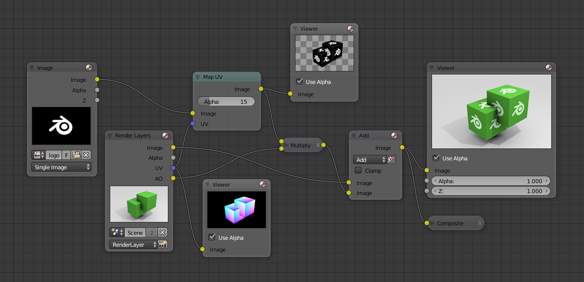
Figure 3: Constructing an image by composing modules in Blender3D. Taken from https://docs.blender.org/manual/en/latest/compositing/introduction.html, CC BY-SA.

2 Overview of OpenRefine

Let us now get into more detail about how OpenRefine works. Loading a data source into OpenRefine creates a project, which consists of a simple data table: it is a collection of rows and columns. To each row and column, a value (possibly null) is associated.

Family name	Given name	Donation
Green	Amanda	25€
Dawson	Rupert	12€
de Boer	John	40€
Tusk	Maria	3€

(a) The initial state of the project

Family name	Given name	Full name	Donation
Green	Amanda	Amanda Green	25€
Dawson	Rupert	Rupert Dawson	12€
de Boer	John	John de Boer	40€
Tusk	Maria	Maria Tusk	3€

(b) Applying an operation to create the Full name column

Family name	Given name	Full name	Donation
GREEN	Amanda	Amanda Green	25€
DAWSON	Rupert	Rupert Dawson	12€
DE BOER	John	John de Boer	40€
TUSK	Maria	Maria Tusk	3€

(c) Applying an operation to capitalize the Family name column

(d) The workflow represented as a string diagram. Operation $\alpha$ is concatenation, operation $\beta$ is capitalization

Figure 4: Example of an OpenRefine project in its successive states, with the corresponding string diagram

The user can then apply operations on this table. Applying an operation will change the state of the table, usually by performing the same transformation for each row in the table. Example of operations include removing a column, reordering columns, normalizing the case of strings in a column or creating a new column whose values are obtained by concatenating the values in other columns. Users can configure these operations with the help of an expression language which lets them derive the values of a new column from the values in existing columns.

Unlike spreadsheet software, such expressions are fully evaluated when stored in the cells that they define: at each stage of the transformation process, the values in the table are static and will not be updated further if the values they were derived from change in the future. For instance, in the sample project of Figure 4, the first operation creates a Full name column by concatenating the Given name and Family name columns. Applying a second operation to capitalize the Family name column does not change the values in the Full name column.

Another difference with spreadsheet software, where it is possible to reference any cell in the expression defining a cell, is that OpenRefine’s expression language only lets the user access values from the same row. For instance, in the same example project of Figure 4, spreadsheet software would make it easy to compute the sum of all donations in a final row. This is not possible in OpenRefine as this would amount to computing the value of a cell from the value of other cells outside of its own row.

In other words, operations in OpenRefine are applied row-wise and are stateless: no state is retained between the processing of rows. It is therefore simple to parallelize these operations, as they amount to a pure map on the list of rows. This is a simplification: in reality, there are violations of these requirements (for instance, OpenRefine offers a sorting operation, and a records mode which introduces a restricted form of non-locality). Due to the limited space we do not review these violations here.

3 Elementary model of OpenRefine workflows

So far, OpenRefine fits neatly in the dataflow paradigm presented in Section 1. One can view each column of a project as a data stream, which can be assigned a type $t\in T$: in our example project, the first two columns are string-valued and the third contains monetary values. These data streams are synchronous: the values they contain are aligned to form rows. An operation $\alpha\in O$ can be seen as reading values from some columns and writing new columns as output. Because of the synchronicity requirement, an operation really is just a function from tuples of input values on the columns it reads to values on the column it writes.

The schema of a table, which is the list of its column types, can be naturally represented by the product of the objects representing its column types. In the example of Figure 4, the initial table is therefore represented by $S\times S\times M$, where $S$ is the type of strings and $M$ of monetary values. Let us call $\alpha:S\times S\rightarrow S$ the first concatenation operation and $\beta:S\rightarrow S$ the second capitalization operation. Figure 4(d) shows a string diagram which models the workflow of Figure 4.

Definition 3.

The category $\mathcal{E}$ of table schema and elementary OpenRefine workflows between them is the free cartesian category generated by a set of datatypes $D$ as objects and a set of operations $O$ as morphisms.

This modelling of OpenRefine workflows makes it easy to reason about the information flow in the project. It is possible to rearrange the operations using the axioms of a cartesian category to show that two workflows produce the same results. We could add some generating equations between composites of the generating operations, such as operations which commute even when executed on the same column for instance.

Without loss of generality, we can assume that the generating operations all have a single generating datatype as codomain, as the cartesian structure makes it possible to represent generic operations as composites of their projections. Under these conditions, morphisms of $\mathcal{E}$ can be rewritten to a normal form, illustrated in Figure 5.

$=$

Figure 5: A diagram in $\mathcal{E}$ and its normal form

Lemma 1.

Any morphism $m\in\mathcal{E}$ can be written as a vertical composite of three layers: the first one only contains copying and discarding morphisms, the second only symmetries and the third only generating operations (identities are allowed at each level).

All three slices in the decomposition above can be further normalized: for instance, the cartesian slice can be expressed in left-associative form, the exchange slice is determined by the permutation it represents and the operation slice can be expressed in right normal form [delpeuch2018normalization]. This gives a simple way to decide the equality of diagrams in $\mathcal{E}$. Of course, deciding equality in a free cartesian category just amounts to comparing tuples of terms in universal algebra. We are only formulating it as a graphical rewriting procedure to lay down the methodoly for the next section.

4 Model of OpenRefine workflows with facets

One key functionality of OpenRefine that we have ignored so far is its facets. A facet on a column gives a summary of the value distribution in this column. For instance, a facet on a column containing strings will display the distinct strings occurring in the column and their number of occurences. A numerical facet will display a histogram, a scatterplot facet will display points in the plane, and so on.

Beyond the use of facets to analyze distributions of values, it is also possible to select particular values in the facet, which selects the rows where these values are found. It is then possible to run operations on these filtered rows only. So far our operations ran on all rows indiscriminately, so we need to extend our model to represent operations applied to a filtered set of rows.

We assume from now on a set $F$ of filters in addition to our set of operations $O$. Each filter $f\in F$ is associated with an object $T_{\_}f\in\mathcal{E}$, the type of data that it filters on. Each filter can be thought of as a boolean expression that can be evaluated for each value $v\in T_{\_}f$, determining if the value is included or excluded by the filter. The type $T_{\_}f$ is not required to be atomic: for instance, in the case of a scatterplot filter, two numerical columns are read.

Definition 4.

Let $\mathcal{F}$ be the free co-cartesian category generated as follows. We denote by $[A_{\_}1,\dots,A_{\_}n]$ the product of objects $A_{\_}1,\dots,A_{\_}n$ in $\mathcal{F}$ to distinguish it from the product $\times$ in $\mathcal{E}$. For each object $T\in\mathcal{E}$, $[T]\in\mathcal{F}$ is a generator. Morphism generators are:

1. For each morphism $\alpha\in\mathcal{E}(T,U)$, there is a generator $[\alpha]:[T]\rightarrow[U]$.

2. For each filter $f$ and object $U\in\mathcal{E}$, there is a generator $[f\times U]:[T_{\_}f\times U]\rightarrow[T_{\_}f\times U,T_{\_}f\times U]$.

For each object $T\in\mathcal{E}$, we call $J_{\_}T:[T,T]\rightarrow[T]$ and $E_{\_}T:[]\rightarrow[T]$ the comultiplication and counit provided by the co-cartesian structure.

The axioms satisfied by these generators are stated graphically in Figure 7, with the notations introduced in Figure 6. In addition to these axioms, we require that $[g]\circ[f]=[g\circ f]$ (which is tautological graphically). In other words, $\mathcal{E}$ embeds into $\mathcal{F}$ functorially (but that functor is not monoidal).

The definition above can be interpreted intuitively as follows. An object in $\mathcal{E}$ represents the schema of a table (the list of types of its columns). An object of $\mathcal{F}$ is a list of objects of $\mathcal{E}$, so it represents a list of table schemata. As will be made clear by the semantics defined in the next section, a morphism in $\mathcal{F}:[U,V]\mapsto[W,Z]$ should be thought of as a function mapping disjoint tables of respective schemata $U$ and $V$ to disjoint tables of respective schemata $W$ or $Z$, and row-wise so: depending on its values, a row can end up in either of the output tables. This makes it therefore possible to represent filters as morphisms triaging rows to disjoint tables. A filter $[f\times U]$ operates on tables of schema $T_{\_}f\times U$, and only reads values from the first component to determine whether to send the row to the first or second output table. This treatment of a boolean predicate $A\rightarrow 2$ as a morphism $A\rightarrow A+A$ is similar to that of effectus theory [cho2015introduction]. The comultiplication $J_{\_}T$ is a union, merges two tables of identical schemata together. The counit $E_{\_}T$ is the empty table.

Given the two nested list structures in objects of $\mathcal{F}$, it is natural to represent them as two-dimensional objects, and morphisms of $\mathcal{F}$ become three-dimensional objects, as shown in Figure 6. Figure 7 states the relations satisfied by these generators using this convention.

(a) Operation $[\alpha]:[A\times B]\to[C\times D]$

(b) Filter $[f\times U]:[T_{\_}f\times U]\rightarrow[T_{\_}f\times U,T_{\_}f\times U]$

(c) Union $J_{\_}T:[T,T]\rightarrow[T]$

(d) Empty table: $E_{\_}T:[]\rightarrow[T]$

Figure 6: Generators of $\mathcal{F}$

$=$

(a) Merging a filter immediately does nothing

$=$

(b) Filters commute even with a common column

$=$

(c) Disjoint filters and operations commute

$=$

(d) Copying and filtering commute

$=$

$=$

(e) Filters do not modify data

Figure 7: Axioms of $\mathcal{F}$

OpenRefine workflows with filters can be represented by morphisms $\mathcal{F}$. For the converse, we first show that morphisms of $\mathcal{F}$ can be represented in normal form thanks to the following decomposition.

Lemma 2.

Let $m\in\mathcal{F}([A],[B])$ be a morphism with one input sheet and one output sheet. There exists a decomposition $m=z\circ y\circ x\circ[w]$ such that $w\in\mathcal{E}$, $x$ only contains filters, $y$ only contains discarding morphisms, and $z$ only contains unions.

This decomposition can be used to show that all such morphisms arise from OpenRefine workflows, despite the fact that some generators cannot be interpreted as such individually. As stated, this lemma does not provide normal forms yet, as the order of filters in $x$ is not determined. We will see in the proof of Theorem 1 how this can be addressed.

5 Semantics and completeness

We can give set-valued semantics to $\mathcal{E}$ and $\mathcal{F}$ and obtain completeness theorems for our axiomatization of OpenRefine workflows.

Definition 5.

A valuation $V$ is given by:

1. a set $V(T)$ for each basic datatype $T\in\mathcal{E}$;

2. a function $V(\alpha):V(A)\rightarrow V(B)$ for each generator $\alpha\in\mathcal{E}(A,B)$, where $V(A)$ is the cartesian product of the valuations of the basic types in $A$;

3. a subset $V(f)\subset V(T_{\_}f)$ for each filter $f$.

Any valuation $V$ defines a functor $V^{*}:\mathcal{F}\rightarrow\mathbf{Set}$ as follows:

$$V^{*}([A\times\dots\times B,\dots,C\times\dots\times D]) =(V(A)\times\dots\times V(B)\sqcup\dots\sqcup(V(C)\times\dots\times V(D))$$

$$V^{*}([\alpha]) =V(\alpha)$$

$$V^{*}([f\times U]) =((x,u)\mapsto\operatorname{inj}_{\_}i(x,u))\text{ with $i=1$ if $x\in V(f)$ else $i=2$}$$

$$V^{*}([J_{\_}T]) =(\operatorname{inj}_{\_}i(x)\mapsto x)$$

$$V^{*}([E_{\_}T]) =(theinitialmorphismfromtheemptyset)$$

Using the decomposition of Lemma 2, we can then show the completeness of our axiomatization for these semantics:

Theorem 1.

Let $d,d^{\prime}\in\mathcal{F}([A],[B])$ be diagrams. Then $d=d^{\prime}$ by the axioms of $\mathcal{F}$ if and only if $V^{*}(d)=V^{*}(d^{\prime})$ for any valuation $V$.

The proof of this theorem is given in appendix. Broadly speaking, it goes by building a valuation where values are syntactic terms, such that a value encodes its entire own history through the processing pipeline. These syntactic values are associated with contexts which record the validity of filter expressions. The decomposition of Lemma 2 is then used to compute normal forms for diagrams, which can be related to the evaluation of the diagram with the syntactic valuation. These normal forms can be computed using a simple diagramatic rewriting strategy, so this also solves the word problem for this signature.

We conjecture that this result generalizes to arbitrary morphisms in $\mathcal{F}$, with multiple input and output tables. However, all OpenRefine workflows have one input and one output table, so the theorem already covers these.

6 Conclusion

We have presented a complete axiomatization of the core data model of OpenRefine. This gives a diagrammatic representation for workflows and an algorithm to determine if two workflows are equivalent up to these axioms.

As future work, this visualization suggested by the categorical model could be implemented in the tool itself. This would make workflows easier to inspect, share and re-arrange. This representation could also be the basis of a more profound overhaul of the implementation of the data model, which would make workflow execution more scalable. The axiomatization could also be extended to account for algebraic equations involving the operations, although it seems hard to preserve completeness and decidability for non-trivial equational theories. Finally, the model could be extended to account for a larger class of operations, for instance order-dependent ones such as sorting, or operations which are not applied row-wise (using OpenRefine’s record mode).

7 Acknowledgements

We thank David Reutter, Jamie Vicary and the anonymous reviewers for their helpful feedback on the project. The author is supported by an EPSRC Studentship.

relax

Proof.

relax∎

relaxrelax relaxaxp@lemmarp [2]relaxaxp@fw@rirelaxrelaxrelaxaxp@lemmarp

relaxaxp@oldproof First, any empty tables $E-T$ in the diagram can be eliminated as co-cartesian units, just like discarding morphisms can be eliminated in the cartesian case (Section 3).

We then move all operations, copy morphisms and exchanges in $\mathcal{E}$ up to the first sheet. Operations and copy morphisms can be moved past unions and empty tables by the properties of the co-cartesian structure. Although Equation 7(c) can only be used for operations and filters applied to disjoint columns, it can be combined with Equation 7(d) to commute any operation and filter, possibly leaving discarding morphisms behind:

$=$

$=$

$=$

$=$

This lets us push all operations up, obtaining the first part of the factorization: $m=\phi\circ[w]$ with $w\in\mathcal{E}$ and $\phi$ consists of filters, unions, discarding morphisms and exchanges in $\mathcal{F}$.

Unions can be moved down by naturality, obtaining $m=z\circ\phi^{\prime}\circ[w]$ where $\phi^{\prime}$ only consists of filters, discarding morphisms and exchanges in $\mathcal{F}$. Then, all exchanges in $\phi^{\prime}$ can be moved down by naturality and absorbed by $z$. Finally, all discarding morphisms can be moved down past the filters using Equation 7(c). relaxaxp@oldproof relaxaxp@thmrp [1]relaxaxp@fw@riirelaxrelaxrelaxaxp@thmrp

relaxaxp@oldproof We can check that all equations of Figure 7 preserve the semantics under any valuation, so if two diagrams are equivalent up to these axioms, then their interpretations are equal. For the converse, let us first introduce a few notions. We use a countable set of variables $V=\{x_{\_}1,x_{\_}2,x_{\_}3,\dots\}$.

Definition 6.

The set $\Theta$ of terms is defined inductively: it contains the variables $V$, and for each an operation symbol $\alpha\in O$ of input arity $n$ and output arity $p$, it contains the terms from $\alpha(t_{\_}1,\dots,t_{\_}n)[1]$ to $\alpha(t_{\_}1,\dots,t_{\_}n)[p]$. These terms represent the projections of the operation applied to the input terms.

The set $\Theta_{\_}n$ of terms over $n$ variables is the set of terms where only variables from $\{x_{\_}1,\dots,x_{\_}n\}$ are used. Given $t\in\Theta_{\_}n$ and $u_{\_}1,\dots,u_{\_}n\in\Theta_{\_}m$ we can substitute simultaneously all the $x_{\_}i$ by $u_{\_}i$, which we denote by $t[u_{\_}1,\dots,u_{\_}n]$. For instance, let $t=\alpha(\beta(x_{\_}1,x_{\_}3)[2],x_{\_}1)[1]$ and $u_{\_}1=x_{\_}3$, $u_{\_}2=x_{\_}4$ and $u_{\_}3=\gamma(x_{\_}1)[3]$. Then $t[u_{\_}1,u_{\_}2,u_{\_}3]=\alpha(\beta(x_{\_}3,\gamma(x_{\_}1)[3])[2],x_{\_}3)[1]$.

Definition 7.

An atomic filter formula (AFF) over $n$ variables is given by a filter symbol $f$ and terms $t_{\_}1,\dots,t_{\_}a\in\Theta_{\_}n$ where $a$ is the arity of $f$. It is denoted by $f(t_{\_}1,\dots,t_{\_}a)$ and represents the boolean condition evaluated on the given terms.

We denote by $\Phi$ the set of all atomic filter formulae. Similarly, $\Phi_{\_}n$ is the set of AFF over $n$ variables.

Definition 8.

A conjunctive filter formula (CFF) over $n$ variables is a given by a finite set $A\subset\Phi_{\_}n\times\mathbb{B}$ of pairs of atomic filter formulae and booleans, called clauses, such that no atomic filter formula appears with both booleans. Such a set represents the conjunction of all its clauses, negated when their associated boolean is false.

Two CFF $A$ and $B$ are disjoint if they contain the same atomic filter formula with opposite booleans. Otherwise, we can form the conjuction $A\land B$, which is the CFF with clauses $A\cup B$.

We denote by $\Delta$ the set of CFF and $\Delta_{\_}n$ that of those over $n$ variables. A CFF is represented as a conjuctive clause in boolean logic, such as $f(x_{\_}1,\alpha(x_{\_}3,x_{\_}2)[1])\land\overline{g}(x_{\_}3)$.

Definition 9.

A truth table $t$ on $n$ variables and $p$ outputs, denoted by $t:n\rightarrow p$, is a finite set of cases $c\in\Delta_{\_}n\times\Theta_{\_}n^{p}$, such that all the CFF are pairwise disjoint. This represents possible values for an object, depending on the evaluation of some filters.

Truth tables $t,t^{\prime}$ both on $n$ variables and $p$ outputs are disjoint if all the CFF involved are pairwise disjoint. The union of two disjoint truth tables $t,t^{\prime}$, denoted by $t\cup t^{\prime}$, is the union of their cases. The composition of truth tables $t:n\rightarrow p$ and $t^{\prime}:p\rightarrow q$, denoted by $t;t^{\prime}$, is formed of the cases $(c_{\_}i\land c^{\prime}_{\_}j,u^{\prime}_{\_}{j,1}[u_{\_}{i,1},\dots,u_{\_}{i,p}],\dots,u^{\prime}_{\_}{j,q}[u_{\_}{i,1},\dots,u_{\_}{i,p}])$ for all $(c_{\_}i,u_{\_}i)\in t$ and $(c^{\prime}_{\_}j,u^{\prime}_{\_}j)$ such that $c_{\_}i$ and $c_{\_}j$ are compatible.

A collection of truth tables $(t_{\_}i:n\rightarrow p)_{\_}i$ forms a partition if the CFF in them are all disjoint and their disjunction is a tautology. The projection of a truth table $t$ with $p$ outputs on its $k$-th component, $1\leq k\leq k$, denoted by $t[k]$, is given by the cases $(c_{\_}i,u_{\_}{i,k})$ for $(c_{\_}i,u_{\_}i)\in t$. The product of truth tables $t:n\rightarrow p$ and $t^{\prime}:n\rightarrow q$, denoted by $t\otimes t^{\prime}:n\rightarrow p+q$, is given by the cases $(c_{\_}i\land c^{\prime}_{\_}j,u_{\_}i,u^{\prime}_{\_}j)$ for all $(c_{\_}i,u_{\_}i)\in t$ and $(c^{\prime}_{\_}j,u^{\prime}_{\_}j)\in t^{\prime}$ such that $c_{\_}i$ and $c_{\_}j$ are compatible. Two truth tables $t,t^{\prime}:n\rightarrow p$ are equivalent, denoted by $t\sim t^{\prime}$, if all the cases in $t\otimes t^{\prime}$ have value tuples of the form $(v_{\_}1,\dots,v_{\_}p,v_{\_}1,\dots,v_{\_}p)$.

One can check that all the properties and operations on truth tables defined above respect the equivalence relation $\sim$: we will therefore work up to this equivalence in the sequel. We can represent truth tables by their list of cases:

$$f(x_{\_}1)\land g(\gamma(x_{\_}2)[1]) \mapsto(x_{\_}3,\alpha(x_{\_}1,x_{\_}1)[1])$$

$$f(x_{\_}1)\land\overline{g}(\gamma(x_{\_}2)[1]) \mapsto(x_{\_}2,\alpha(x_{\_}1,x_{\_}1)[1])$$

$$\overline{f}(x_{\_}1) \mapsto(\beta(x_{\_}2,x_{\_}3)[2],x_{\_}1)$$

With the syntactic objects just defined, we can now define semantics for $\mathcal{F}$ that are independent from any valuation. The morphisms will be families of truth tables, which can interpret the generators of $\mathcal{F}$.

Definition 10.

The category $\mathcal{T}$ is a symmetric monoidal category with $\operatorname{Ob}(\mathcal{T})=\mathbb{N}^{*}$ (lists of natural numbers) and where the monoidal product is given by concatenation.

A morphism $t\in\mathcal{T}([a_{\_}1,\dots,a_{\_}n],[b_{\_}1,\dots,b_{\_}m])$ is a collection $t_{\_}{i,j}$ of truth tables, $1\leq i\leq n$ and $1\leq j\leq m$, such that $t_{\_}{i,j}$ is of type $a_{\_}i\rightarrow b_{\_}j$, and for each $i$, $(t_{\_}{i,j})_{\_}j$ is a partition. Furthermore we require that $m>0$ unless $n=0$.

Given morphisms $t:[a_{\_}1,\dots,a_{\_}n]\rightarrow[b_{\_}1,\dots,b_{\_}m]$ and $u:[b_{\_}1,\dots,b_{\_}m]\rightarrow[c_{\_}1,\dots,c_{\_}p]$, the composite $t;u$ is given by $(t;u)_{\_}{i,k}=\bigcup_{\_}{1\leq j\leq m}(t_{\_}{i,j};u_{\_}{j,k})$.

The tensor product of $t:[a_{\_}1,\dots,a_{\_}n]\rightarrow[b_{\_}1,\dots,b_{\_}m]$ and $u:[c_{\_}1,\dots,c_{\_}p]\rightarrow[d_{\_}1,\dots,d_{\_}q]$ is the morphism $v:[a_{\_}1,\dots,a_{\_}n,c_{\_}1,\dots,c_{\_}p]\rightarrow[b_{\_}1,\dots,b_{\_}m,d_{\_}1,\dots,d_{\_}q]$ defined by $v_{\_}{i,j}=t_{\_}{i,j}$ for $i\leq n$ and $j\leq p$, $v_{\_}{i,j}=u_{\_}{i-n,j-m}$ for $i>n$ and $j>p$, and the empty truth table otherwise.

The identity $1$ on $[a_{\_}1\dots,a_{\_}n]$ is given by $1_{\_}i=\top\mapsto(x_{\_}1,\dots,x_{\_}n)$.

Figure 8: Definition of $P:\mathcal{F}\rightarrow\mathcal{T}$

There is a functor $P:\mathcal{F}\rightarrow\mathcal{T}$ defined on objects by $P([A_{\_}1\times\dots\times A_{\_}n])=[n]$ and on morphisms by Figure 8. One can check that it respects the axioms of $\mathcal{F}$.

Lemma 3.

The functor $P$ is faithful.

Proof.

We show this by relating the image $P(d)$ of a diagram to its decomposition given by Lemma 2. As such, this decomposition does not give a normal form, as the order of the filters remains unspecified. However, successive filters can be swapped freely:

$=$

$=$

Let us pick an arbitrary order on $\Phi$, the set of atomic filter formulae. In a diagram $d$ decomposed by Lemma 2 as $z\circ y\circ x\circ[w]$, Each occurence of a filter in $x$ can be associated with an AFF defined by the filter symbol for the filter and the term obtained from the wires read from $w$. Commuting filters as above does not change their corresponding AFF. Therefore this determines an order on the filters occurring in $x$. We can rearrange the filters so that $f$ appears above $g$ if their corresponding AFFs are ordered accordingly. This will add new exchanges and unions in $x$, but we can use Lemma 2 a second time to push these to their part of the decomposition, as this procedure does not reorder the filters.

The rest of the decomposition can be normalized too: unions can be normalized by associativity, and any discarding morphism that is present in all sheets of $y$ and discards a wire not read by any filter in $x$ can be pushed up into $w$, which can be normalized as a morphism in $\mathcal{E}$.

From such a normalized decomposition, we can read out the truth table $P(d)$ directly. Each sheet in $y$ corresponds to a case of $P(d)$, whose condition is determined by the conjunction of all the AFFs of the filters leading to it, with the appropriate boolean depending on the side of the filter they are on. Therefore, if $P(d)=P(d^{\prime})$, then $d=d^{\prime}$. ∎

Definition 11.

The syntactic valuation $S$ is defined as follows. For each basic datype $T$, $S(T)=\Theta\times 2^{\Phi}+\{\bot\}$. In other words, a value can be either a term together with a context of true atomic filter formulae, or an inconsistent value $\bot$.

For each facet $f$, $S(f):(C,t)\mapsto f(t)\in C$: a facet is true if it belongs to the context.

For each operation $\alpha:T_{\_}1\times\dots\times T_{\_}n\rightarrow U_{\_}1\times\dots\times U_{\_}m$,

$$(\alpha):((C,t_{\_}1),\dots,(C,t_{\_}n)) \mapsto((C,\alpha(t_{\_}1,\dots,t_{\_}n)[1],\dots,\alpha(t_{\_}1,\dots,t_{\_}n)[m]))$$

anything else $$\mapsto\bot$$

There is a functor $\Pi:\mathcal{T}\rightarrow\mathbf{Set}$, defined on objects by $\Pi([n_{\_}1,\dots,n_{\_}p])=(\Theta\times 2^{\Phi}+\{\bot\})^{n_{\_}1}\sqcup\dots\sqcup(\Theta\times 2^{\Phi}+\{\bot\})^{n_{\_}p}$. Given a morphism $t:n\rightarrow p$, we define $\Pi(t)(\operatorname{inj}_{\_}i(x))$ as follows. If $x$ contains any $\bot$ or if the contexts in it are not all equal, then $\Pi(t)(\operatorname{inj}_{\_}i(x))=\operatorname{inj}_{\_}1((\bot,\dots,\bot))$. Otherwise, as the truth tables $(t_{\_}{i,j})_{\_}j$ form a partition, there is a single case $(C,y)$ in all of them such that the associated CFF is true in the common context $C$. Let $j$ be the output index of its truth table: we set $\Pi(t)(\operatorname{inj}_{\_}i(x))=\operatorname{inj}_{\_}j(y[x])$. One can check that this defines a monoidal functor.

Lemma 4.

The functor $\Pi$ is faithful.

Proof.

For simplicity, let us concentrate on the case of morphisms $t,t^{\prime}:[n]\rightarrow[p]$: this is the only case that is actually needed to prove the completeness theorem, and the general case is similar. If $\Pi(t)=\Pi(t^{\prime})$, then consider $t\otimes t^{\prime}:n\rightarrow 2p$. For each case $(f,u,u^{\prime})\in t\otimes t^{\prime}$, with $f$ a CFF and $u,u^{\prime}$ tuples of terms, $(f,u)=\Pi(t)(f,x_{\_}1,\dots,x_{\_}n)=\Pi(t^{\prime})(f,x_{\_}1,\dots,x_{\_}n)=(f,u^{\prime})$, so $u=u^{\prime}$. Therefore $t\sim t^{\prime}$. ∎

Finally, combining Lemma 3 and Lemma 4, we obtain that $\Pi\circ P:\mathcal{F}\rightarrow\mathbf{Set}$ is faithful. But in fact $\Pi\circ P=S^{*}$, the functor arising from the valuation $S$. So, if two diagrams $d,d^{\prime}\in\mathcal{F}$ give equal interpretations under any valuation $V$, then it is in particular the case for $V=S$, and by faithfulness of $S^{*}$, $d=d^{\prime}$. relaxaxp@oldproof

References

- [1]
- [2] Kenta Cho, Bart Jacobs, Bas Westerbaan & Abraham Westerbaan (2015): An Introduction to Effectus Theory. arXiv:1512.05813 [quant-ph].
- [3] Bob Coecke (2010): Quantum Picturalism. Contemporary Physics 51(1), pp. 59–83, 10.1080/00107510903257624.
- [4] Antonin Delpeuch & Jamie Vicary (2018): Normalization for Planar String Diagrams and a Quadratic Equivalence Algorithm. arXiv:1804.07832 [cs].
- [5] N. Halbwachs, P. Caspi, P. Raymond & D. Pilaud (1991): The Synchronous Data Flow Programming Language LUSTRE. Proceedings of the IEEE 79(9), pp. 1305–1320, 10.1109/5.97300.
- [6] Thomas T. Hildebrandt, Prakash Panangaden & Glynn Winskel (2004): A Relational Model of Non-Deterministic Dataflow. Mathematical Structures in Computer Science 14(5), pp. 613–649, 10.1017/S0960129504004293.
- [7] David Huynh, Tom Morris, Stefano Mazzocchi, Iain Sproat, Martin Magdinier, Thad Guidry, Jesus M. Castagnetto, James Home, Cora Johnson-Roberson, Will Moffat, Pablo Moyano, David Leoni, Peilonghui, Rudy Alvarez, Vishal Talwar, Scott Wiedemann, Mateja Verlic, Antonin Delpeuch, Shixiong Zhu, Charles Pritchard, Ankit Sardesai, Gideon Thomas, Daniel Berthereau & Andreas Kohn (2019): OpenRefine. 10.5281/zenodo.595996.
- [8] Gilles Kahn (1974): The Semantics of a Simple Language for Parallel Programming. Information processing 74, pp. 471–475.
- [9] K. M. Kavi, B. P. Buckles & U. N. Bhat (1987): Isomorphisms Between Petri Nets and Dataflow Graphs. IEEE Transactions on Software Engineering SE-13(10), pp. 1127–1134, 10.1109/TSE.1987.232854.
- [10] José Meseguer, Ugo Montanari & Vladimiro Sassone (1992): On the Semantics of Petri Nets. In W.R. Cleaveland, editor: CONCUR ’92, 630, Springer Berlin Heidelberg, pp. 286–301, 10.1007/BFb0084798.
- [11] Carl Adam Petri (1966): Communication with Automata, p. 97.
- [12] Vaughn Pratt (1991): Modeling Concurrency with Geometry. In: Proceedings of the 18th ACM SIGPLAN-SIGACT Symposium on Principles of Programming Languages - POPL ’91, ACM Press, Orlando, Florida, United States, pp. 311–322, 10.1145/99583.99625.
- [13] P. Selinger (2010): A Survey of Graphical Languages for Monoidal Categories. In Bob Coecke, editor: New Structures for Physics, Lecture Notes in Physics 813, Springer Berlin Heidelberg, pp. 289–355, 10.1007/978-3-642-12821-94.
- [14] Eugene W. Stark (1991): Dataflow Networks Are Fibrations, 10.1007/BFb0013470. In David H. Pitt, Pierre-Louis Curien, Samson Abramsky, Andrew M. Pitts, Axel Poigné & David E. Rydeheard, editors: Category Theory and Computer Science, Lecture Notes in Computer Science, Springer Berlin Heidelberg, pp. 261–281.
- [15] Edward Walker, Weijia Xu & Vinoth Chandar (2009): Composing and Executing Parallel Data-Flow Graphs with Shell Pipes. In: Proceedings of the 4th Workshop on Workflows in Support of Large-Scale Science - WORKS ’09, ACM Press, Portland, Oregon, pp. 1–10, 10.1145/1645164.1645175.
relax
Proof.
relax∎