Galaxy-Galaxy Lensing in HSC: Validation Tests and the Impact of Heterogeneous Spectroscopic Training Sets

Abstract

Although photometric redshifts (photo-$z$’s) are crucial ingredients for current and upcoming large-scale surveys, the high-quality spectroscopic redshifts currently available to train, validate, and test them are substantially non-representative in both magnitude and color. We investigate the nature and structure of this bias by tracking how objects from a heterogeneous training sample contribute to photo-$z$ predictions as a function of magnitude and color, and illustrate that the underlying redshift distribution at fixed color can evolve strongly as a function of magnitude. We then test the robustness of the galaxy-galaxy lensing signal in 120 deg² of HSC-SSP DR1 data to spectroscopic completeness and photo-$z$ biases, and find that their impacts are sub-dominant to current statistical uncertainties. Our methodology provides a framework to investigate how spectroscopic incompleteness can impact photo-$z$-based weak lensing predictions in future surveys such as LSST and WFIRST.

1 Introduction

Between the surface of last scattering ($z\sim 1100$) and the present day ($z=0$), the paths of all observed photons have been gravitationally influenced by the intervening “cosmic web” of matter. This gravitational lensing, and particularly weak lensing, is sensitive to the growth of structure and expansion history of the Universe and serves as a key probe of cosmology (e.g., see review by Mandelbaum, 2018). In addition, weak lensing serves as an effective complementary technique to other cosmological probes (e.g., the Cosmic Microwave Background or Type Ia supernovae) by helping to break degeneracies between cosmological parameters and providing constraints on the growth of large scale structure (e.g., DES Collaboration et al., 2017; Hildebrandt et al., 2018; Hikage et al., 2018, for some recent cosmic shear results).

The determination of accurate photometric redshifts (photo-$z$’s) is a key challenge for deep lensing surveys. While shallow surveys ($i<24$) can obtain spectroscopic follow-up for representative samples, deeper surveys face tougher challenges. In this paper, we focus on the challenges of deriving photo-$z$’s for the first year source catalog of the HSC survey which reaches an $i$-band depth of $\sim 26$ AB magnitudes. As a precursor to LSST, the HSC-SSP survey is a crucial testing ground for photo-$z$ methods that will be applied for future precision cosmology analyses.

At the depths probed by HSC, there is a lack of adequate representative spectroscopic redshifts (spec-$z$’s) available for training, validating, and testing photo-$z$ methods (Masters et al., 2015; Tanaka et al., 2018). As a result, the HSC photo-$z$ team instead supplements spec-$z$’s taken from a variety of public surveys with grism/prism-based redshifts (g/prism-$z$’s) along with photo-$z$’s derived from deep, many-band photometry when training various photo-$z$ algorithms and validating their performance. These unavoidable choices lead to a heterogeneous training set spanning a wide range of possibly redshift “quality”.

Although mixing spec-$z$’s and high-quality alternatives will likely occur in future surveys, the impact of using such a heterogeneous mixture on weak lensing has not yet been extensively explored. While the lack of high-quality spec-$z$’s in regions of color and magnitude space makes it difficult to validate photo-$z$ performance in those regions independently of the assumptions used to generate them, supplementing spec-$z$’s in these regions with other methods that rely more heavily on these assumptions (see, e.g., Bezanson et al., 2016) will not alleviate this problem. This means that performance in these regions remains a “known unknown” that is difficult to directly validate. This problem is particularly acute for future cosmology surveys hoping to derive unbiased photo-$z$’s at the sub-percent level to the majority of their faint photometric samples.

Currently, there are several attempts in the literature to try to resolve this issue. These take two broad approaches. The first is an attempt to efficiently collect spec-$z$’s to “fill in” regions of color space that currently do not have available data. The largest systematic approach is the C3R2 survey (Masters et al., 2017), which has so far collected $\sim\,1300$ high-quality spectra in under-populated regions of color-space. The second is to assume that we can use cross-correlations of ensembles of galaxies that span the relevant redshift range, regardless of their color and/or magnitude, to characterize photo-$z$ accuracy for a population of galaxies. This has proven to be promising but is not without challenges (Ménard et al., 2013; Newman et al., 2015; Hoyle & Rau, 2018). Importantly, both of these methods assume that we can use ensembles of galaxies in specific regions of color and/or magnitude space to calibrate photo-$z$ biases and uncertainties.

In this paper, we investigate how the use of heterogeneous training samples affects photo-$z$ performance and galaxy-galaxy (gg) lensing analyses (e.g., Kwan et al., 2017; Leauthaud et al., 2017; Prat et al., 2018) using HSC-SSP data. In §2, we describe the photometry, shear, and redshift data used in this paper. In §3, we investigate the representativeness of current spec-$z$ samples and examine the dependence on color and magnitude. We find strong evidence for evolution in the redshift distribution of galaxies at fixed color as a function of magnitude. This leads us to develop a new framework, described in §4, for computing photo-$z$’s from heterogeneous data that incorporates magnitude dependence and allows us to track how specific training objects contribute to individual photo-$z$ predictions. We investigate the accuracy of photo-$z$ probability density functions (PDFs) computed using this method in §5.

After discussing our photo-$z$ tests, in §6 we outline the framework used for our lensing analysis. In §7, we then test whether our gg lensing measurements are robust to a variety of estimators, quality cuts, and spectroscopic incompleteness. We conclude in §8.

We assume a flat $\Lambda$CDM cosmology whenever appropriate with $\Omega_{\Lambda}=0.7$, $\Omega_{\rm m}=0.3$, and $h=0.7$. All magnitudes in the paper are AB magnitudes (Oke & Gunn, 1983). For our lensing calculations (see §7), we assume physical coordinates to compute $\Delta\Sigma$ in 10 logarithmically spaced bins from 0.05 Mpc to 15 Mpc.

2 Data

2.1 The HSC Survey

The Hyper Suprime-Cam Subaru Strategic Program (HSC-SSP) Survey (Aihara et al., 2018) utilizes the Hyper Suprime-Cam prime-focus camera (Miyazaki et al., 2018; Komiyama et al., 2018; Kawanomoto et al., 2018; Furusawa et al., 2018) on the 8.2 m Subaru telescope at Mauna Kea. The survey has a “wedding cake” construction, with three different area/depth combinations to optimize a variety of science goals: the Wide survey will cover 1400 deg² in $grizy$ to a limiting depth of $i\sim 26$ mag, the Deep survey will cover 26 deg² to $i\sim 27$ mag, and the UltraDeep survey will cover 3.5 deg² to a depth of $i\sim 28$ deg². This work is based on the S16A HSC-SSP internal data release, which covers 136.9  deg² to full Wide depths in all five bands. For more information on the HSC-SSP survey, please see Aihara et al. (2018). For more information on the data processing and pipeline, please see Bosch et al. (2018).

2.2 The weak lensing source sample

Our sample of galaxy sources is selected using the weak lensing cuts outlined in Mandelbaum et al. (2018). In brief, these are a series of quality cuts to ensure that composite model (i.e. CModel) photometry, point spread functions (PSFs), and measured object shapes are reliable. Observations are restricted to $i<24.5$ mag to avoid using data with possibly unreliable shape measurements and to ensure “reasonable” spec-$z$ coverage (although see §3). A “full-depth, full-color” (FDFC) cut was also imposed to eliminate sources that were not observed in all bands to full depth. Objects near bright stars were removed using the updated Arcturus bright star masks described in Coupon et al. (2018), as opposed to the original Sirius masks used in Mandelbaum et al. (2018), as those preserve more galaxies around bright stars. See Mandelbaum et al. (2018) for additional details regarding the construction and validation of the HSC-SSP S16A weak lensing shear catalog.

In addition to these weak lensing cuts, the photo-$z$’s used in this work were only computed for objects with PSF-matched 1.1$\arcsec$ aperture photometry available in all five bands. This effectively imposes an additional de facto cut on the seeing in all five bands. A variety of internal tests have found that this does not introduce a meaningful bias on weak lensing analyses (More et al., in prep.).

2.3 Redshift Training Data

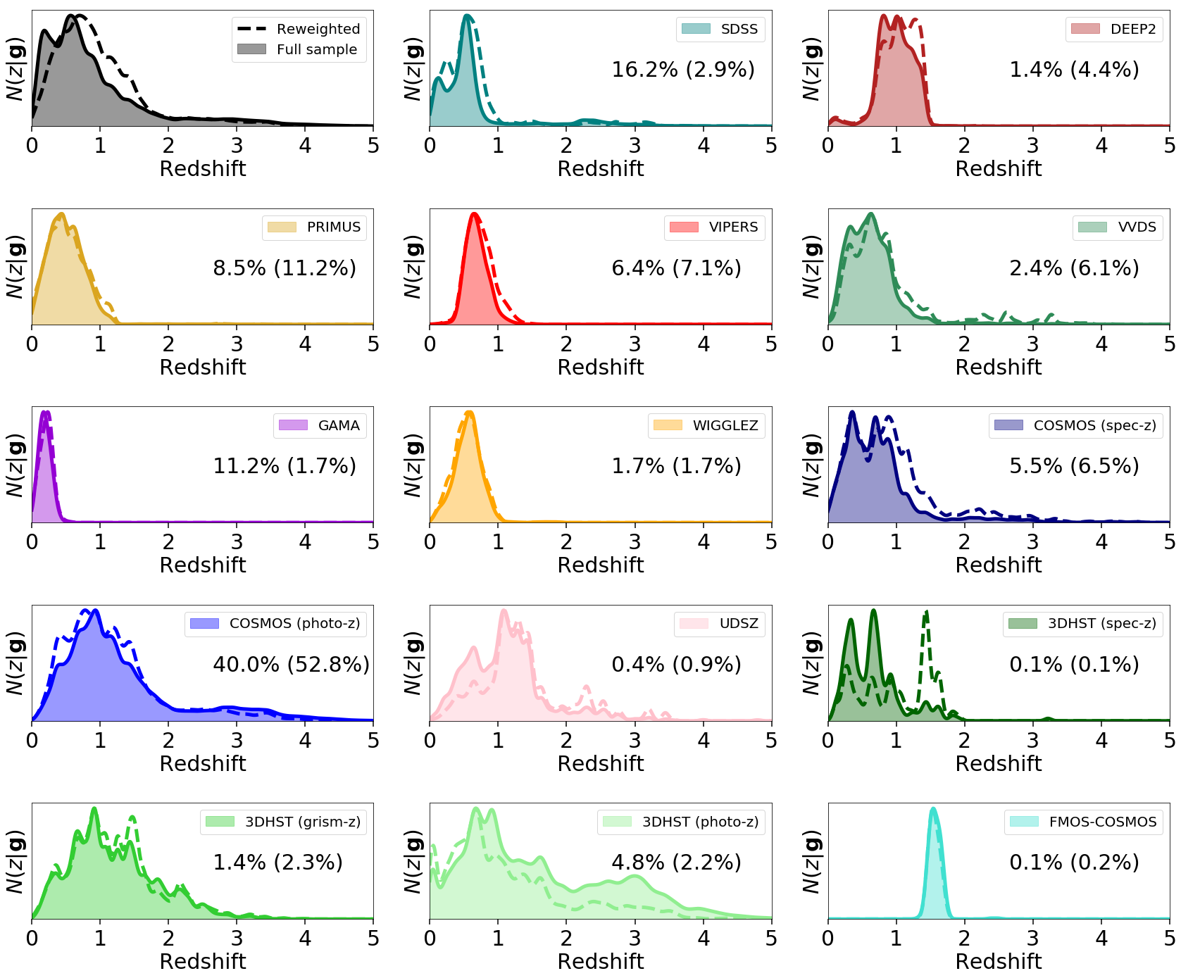
Figure 1: The redshift number density $N(z|\mathbf{g})$ of the objects $\mathbf{g}$ included in the HSC-SSP S16A redshift training set, broken down by survey of origin and source type (if appropriate). Solid lines show the original distribution of objects in the training sample, while dashed curves show the distribution after re-weighting the sample to mimic the color-magnitude distribution of the HSC-SSP S16A weak lensing photometric sample (see §2.3 and §4.4). The raw percentage (reweighted percentage) of the entire training set (gray, top left) comprised of each subsample is also listed in each figure. The color-magnitude weights shift the distribution to higher redshifts and favors deeper surveys with more diverse galaxy populations (e.g., DEEP2, VVDS) over shallower surveys (e.g., GAMA) and those with more limited galaxy population coverage (e.g., SDSS/BOSS). Over 50% of the objects in the weak lensing sample are primarily trained by COSMOS photo-$z$. This illustrates the paucity of current spec-$z$ coverage at the depths probed by the HSC-SSP survey.

The HSC-SSP Wide survey footprint is designed to maximize the overlap with other photometric and spectroscopic surveys while keeping the survey geometry simple. This allows HSC-SSP to exploit a large number of public spec-$z$’s when constructing a redshift training set. In addition, (Ultra)Deep data taken in heavily observed fields such as COSMOS (Scoville et al., 2007) further allows HSC-SSP to include large numbers of fainter objects observed at higher signal-to-noise (S/N). These observations allow for more detailed modeling of the general population observed in the Wide survey, and are especially helpful for fainter sources.

A detailed description of the training sample can be found in Tanaka et al. (2018). We briefly summarize it here. The training set contains spectroscopic, grism, and prism redshifts from a variety of overlapping public surveys including:

• zCOSMOS DR3 (Lilly et al., 2009),

• UDSz (Bradshaw et al., 2013; McLure et al., 2013),

• 3D-HST (Skelton et al., 2014; Momcheva et al., 2016),

• FMOS-COSMOS (Silverman et al., 2015),

• VVDS (Le Fèvre et al., 2013),

• VIPERS PDR1 (Garilli et al., 2014),

• SDSS DR12 (Alam et al., 2015),

• GAMA DR2 (Liske et al., 2015),

• WiggleZ DR1 (Parkinson et al., 2012),

• DEEP2 DR4 (Newman et al., 2013), and

• PRIMUS DR1 (Coil et al., 2011; Cool et al., 2013).

As each survey has its own flagging scheme to indicate redshift confidence, the different schemes were homogenized and used to select “secure” redshifts using the criteria outlined in Tanaka et al. (2018). In addition to these public surveys, a collection of private COSMOS spec-$z$’s were also included exclusively for photo-$z$ training (Mara Salvato & Peter Capak, private communication).

In addition to these spec-$z$’s, grism-$z$’s, and prism-$z$’s, the training set was supplemented with a set of high-quality, many-band photo-$z$’s taken from 3D-HST and COSMOS2015 (Laigle et al., 2016) in order to maintain sufficient magnitude and color coverage down to $i\sim 24.5$ (see §3). Without these photo-$z$’s, the magnitude and color coverage of the training set fails to adequately span the relevant parameter space of the HSC-SSP data used in this analysis. The above heterogeneity in the spec-$z$’s, grism-$z$’s, prism-$z$’s, and many-band photo-$z$’s is one of the motivating reasons for the analysis presented in this work.

Objects were iteratively matched to this catalog within 1$\arcsec$ at (1) UltraDeep, (2) Deep, and (3) Wide HSC-SSP depths in order to take advantage of higher-S/N data when available while avoiding possible duplicates. Our training data ultimately consists of $\sim$ 170k, 37k, and 170k high-quality spec-$z$, g/prism-$z$, and many-band photo-$z$’s, respectively.

As described in Tanaka et al. (2018), to perform accurate cross-validation at HSC-SSP Wide depths, each object was assigned an “emulated” Wide-depth flux error based on the error properties of similar objects observed in the HSC-SSP Wide survey. Objects were also assigned an associated color-magnitude weight using a nearest-neighbor approach based on a representative subset of the weak lensing source sample to account for domain mismatches following the methodology described in §4.4. The original and re-weighted redshift distributions of the HSC-SSP S16A training sample are shown in Figure 1.

3 How Representative are Existing Spectroscopic Redshift Samples?

As discussed in §2.3, spectroscopic “completeness” within our training set varies strongly across magnitude and color. In other words, in a given color-magnitude “bin” the fraction of objects that come from more reliable sources such as spec-$z$’s versus more unreliable sources such as many-band photo-$z$’s can change rapidly.

This behavior is concerning for several reasons. First, spec-$z$’s generally have much smaller (often negligible) errors in redshift measurements compared to photo-$z$’s, so our underlying knowledge of the redshift distribution at fixed magnitude and/or color degrades as the number and/or fraction of spec-$z$’s decreases. Second, it is a well known issue that photo-$z$ PDFs can be mis-calibrated (see, e.g., Tanaka et al. 2018). Third, there may be systematic biases of the redshift distribution of spec-$z$’s relative to photo-$z$’s in a given color-magnitude bin arising from selection effects that arise during the process of data collection. These involve choices that often generate the mismatch in the first place, from prioritizing spectroscopic targets (which often impose magnitude and color biases) to how non-detections are treated (which correlates strongly with redshift).

In particular, many studies assume that these pathological behaviors can be “calibrated out” by matching objects explicitly in terms of color (not magnitude) to obtain a representative spec-$z$ sample (see, e.g., Lima et al., 2008). Surveys such as the Complete Calibration of the Color-Redshift Relation (C3R2) Survey (Masters et al., 2017) have expanded upon this strategy, explicitly sorting possible targets into bins in color space and then pursuing them assuming that spec-$z$’s obtained at fixed color are representative of the entire photometric population in that given color bin.

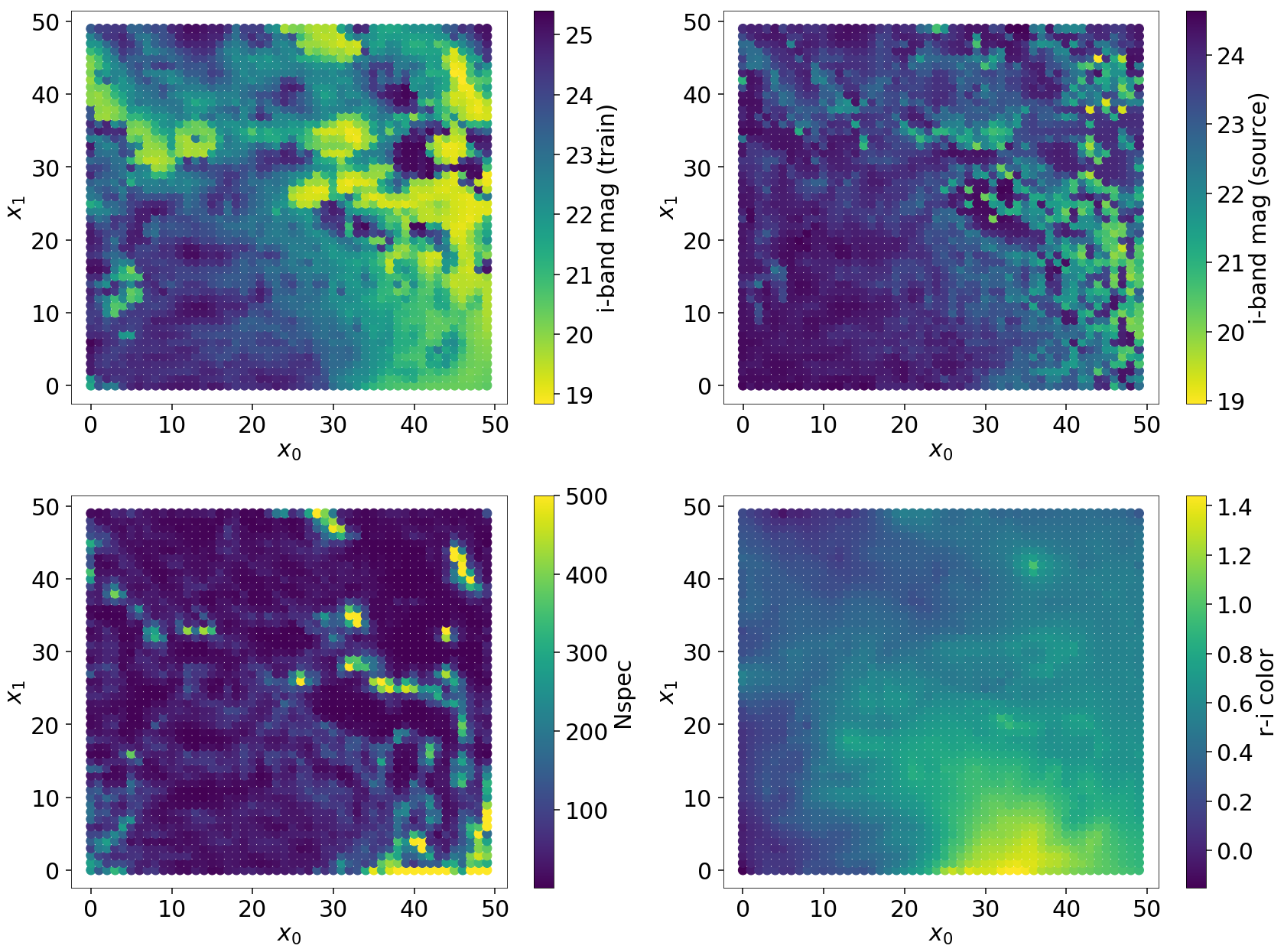
Figure 2: The mean $i$-band magnitude of the training set (top left) and a randomly-selected subset of the weak lensing source catalog (top right), the number of spec-$z$’s (capped at 500; bottom left), and $r-i$ color (bottom right) of the $50\times 50$ Self-Organizing Map (SOM) trained on the HSC-SSP S16A weak lensing photometric sample. The spec-$z$’s in our training sample occupy almost entirely mutually-exclusive regions of magnitude space from the weak lensing photometric sample and have preferentially brighter magnitudes. As with Figure 1, we see that large portions of color/magnitude space do not have sufficient coverage within our dataset, necessitating the use of many-band photo-$z$’s from surveys such as COSMOS to “bridge the gap” when computing photo-$z$’s for HSC-SSP.

While this strategy is efficient, it assumes that the intrinsic redshift distribution $P(z|\mathbf{c})$ at fixed color $\mathbf{c}$ is representative over all relevant magnitudes $m$. This is a strong assumption given that the population of galaxies evolves as a function of redshift and that we expect brighter objects of fixed color to be (on average) at lower redshifts, all else being fixed. We begin by investigating to what degree $P(m_{\rm spec}|\mathbf{c})$ differs from $P(m|\mathbf{c})$ and whether or not these differences are of importance to current lensing surveys.

More formally, this assumption implies that

$$P(z|\mathbf{c}) =\int P(z|\mathbf{c},m)P(m|\mathbf{c})dm$$ (1)

$$\approx\frac{1}{N_{\rm spec}}\sum_{i}K(z|z_{i,{\rm spec}})$$ (2)

where $K(z|z_{i,{\rm spec}})$ is a kernel density estimate (i.e. smoothing scale) for each spec-$z$ where $z_{i,{\rm spec}}$ is a spectroscopic redshift drawn from a particular spec-$z$ distribution $P(m_{\rm spec}|\mathbf{c})\neq P(m|\mathbf{c})$ based on how the data were collected. Note that, in general, (2) is only guaranteed to be approximately valid if all the spec-$z$’s comprise a representative sample from the underlying magnitude distribution at fixed color $P(m|\mathbf{c})$.

To investigate these potential issues in our training sample, we will use manifold learning to sort our training galaxies into regions of color space to investigate possible trends in $P(z|\mathbf{c},m)$. In §3.1, we describe the particular algorithm and procedure used to construct the manifold. In §3.2, we examine several examples of $P(z|\mathbf{c},m)$ and find that there can be significant evolution as a function of magnitude in particular regions of color. Our results imply that current spec-$z$ follow-up programs should be cognizant of these effects in order to avoid biasing photo-$z$ predictions at fixed color. Since the redshift success rate for a given spectrograph may depend on the redshift, at a given magnitude and color bin even surveys that are relatively homogeneously selected may be subject to these subtle biases.

3.1 Manifold Learning and Self Organized Maps

For this study, we use a Self-Organizing Map (SOM; Kohonen, 1982, 2001) to both cluster our data in color space and learn a lower-dimensional 2-D projection that can be used for visualization purposes. We summarize the main features of our specific implementation below, and direct the reader to Carrasco Kind & Brunner (2014a), Masters et al. (2015); Masters et al. (2017), and Speagle & Eisenstein (2017) for more details concerning their applications to photo-$z$’s.

The SOM is an unsupervised machine learning algorithm that projects high-dimensional data onto a lower-dimensional space using competitive training of a (large) set of “nodes” in a way that attempts to preserve general topological features and correlations present in the higher-dimensional data. It consists of a fixed number of nodes $N_{\rm nodes}=\prod_{i=1}^{D}N_{\rm nodes}^{i}$, where the product over $i$ is taken over all dimensions $D$ of the SOM, arranged on an arbitrary $D$-dimensional grid with $N_{\rm nodes}^{i}$ nodes in each dimension. Each node in the grid is assigned a position $\mathbf{x}$ on the SOM and is represented by a particular model $\mathbf{F}(\mathbf{x})$, where $\mathbf{F}$ is the set of observed features. In this paper, these are the set of $grizy$ photometric flux densities comprising a particular galaxy Spectral Energy Distribution (SED) in the HSC filters.

Once the dimensions/shape of the SOM are chosen, training then proceeds as follows:

1. Initialize the node models (most often randomly) and set the current iteration t = 0.

2. Draw (with replacement) a random object $\hat{\mathbf{F}}$ and its associated errors $\bm{\sigma}$ from the input dataset.

3. Compute

   $$\chi^{2}(\mathbf{x})=\sum_{b}\sigma_{b}^{-2}(\hat{F}_{b}-s(\mathbf{x})F_{b}(\mathbf{x}))^{2}$$ (3)

   across all nodes in the SOM over the available bands indexed by $b$, where the scale factor

   $$s=\frac{\sum_{b}\sigma_{b}^{-2}\hat{F}_{b}F_{b}(\mathbf{x})}{\sum_{b}\sigma_{b}^{-2}F_{b}^{2}(\mathbf{x})}$$ (4)

   renormalizes the model SED so that we are fitting in terms of flux density ratios (i.e. colors) rather than flux densities (i.e. magnitudes) directly.

4. Select the best-matching node

   $$\mathbf{x}_{\rm best}=\underset{\mathbf{x}}{\mathrm{argmin}}\left\{\chi^{2}(\mathbf{x})\right\}$$ (5)

   based on the minimum $\chi^{2}(\mathbf{x})$ value.

5. Update the node models $\mathbf{F}(\mathbf{x})\rightarrow\mathbf{F}^{\prime}(\mathbf{x})$ based on a learning rate $\mathcal{A}(t)$ and neighborhood function $\mathcal{H}(\mathbf{x},\mathbf{x}_{\rm best}|t)$ such that

   $$\mathbf{F}^{\prime}(\mathbf{x})=s(\mathbf{x})\mathbf{F}(\mathbf{x})+\mathcal{A}(t)\mathcal{H}(\mathbf{x},\mathbf{x}_{\rm best}|t)(\hat{\mathbf{F}}_{i}-s(\mathbf{x})\mathbf{F}_{i}(\mathbf{x}))$$ (6)

6. If $t\leq N_{\rm iter}$, increment $t$ and repeat starting from (ii).

After training, objects are typically “mapped” onto the SOM by repeating steps (iii) and (iv) for every object in the input dataset, assigning each object to its best-matching node. We use a modified version of this approach where each object $\hat{\mathbf{F}}_{j}$ is instead assigned to a set of nodes along with its corresponding weight $w_{j}(\mathbf{x})\propto e^{-\chi^{2}(\mathbf{x})/2}$ for all nodes with $w_{j}(\mathbf{x})>f_{\min}\max(w_{j}(\mathbf{x}))$. We take $f_{\min}=10^{-3}$, which approximately corresponds to thresholding galaxies that are $\sim 2.5\sigma$ away from the best-fit. This “probabilistic mapping” allows us to better capture the uncertainty in an individual object’s position on the SOM based on its photometric errors, resulting in smoother maps that are less sensitive to sampling noise and photometric errors relative to, e.g., Masters et al. (2017). A detailed discussion of these differences is beyond the scope of this paper and will be explored in future work.

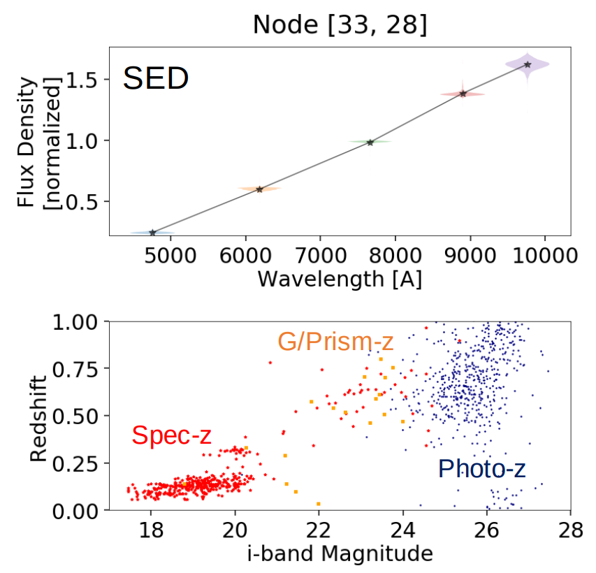
Figure 3: Top: The SED associated with a particular node in the SOM located at position $\mathbf{x}=[33,28]$. The rescaled flux densities of objects associated with the node are shown as “violin plots” around the node SED, weighted according to each object’s relative likelihood of being associated with the node. Bottom: A Monte Carlo realization of the corresponding redshifts of spec-$z$’s (red), g/prism-$z$’s (orange), and many-band photo-$z$’s (blue) and plotted based on their relative likelihood of being associated with the node. We see a clear trend towards higher redshift as a function of magnitude. While some of the evolution at fainter magnitudes is due to intra-bin scatter from photometric uncertainty, this effect is minimal at brighter magnitudes where the trend is clearest.

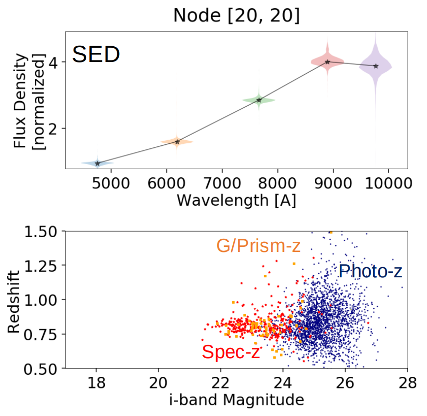
Figure 4: Top: As Figure 3, but for a particular node located at position $\mathbf{x}=[20,20]$ in the SOM. Bottom: Monte Carlo realizations from the redshift PDFs of sources associated with the node following Figure 3. In contrast to 3, for these particular colors at most magnitudes the overall behavior is consistent with having a non-evolving intrinsic redshift distribution.

We choose our SOM to be 2-D with a $50\times 50$ grid of nodes, and train it on the weak lensing source catalog photometry following the steps above for $N_{\rm iter}=10^{5}$ iterations, which we find is enough to ensure the median $\chi^{2}(\mathbf{x}_{\rm best})$ value for objects across our map is approximately the number of colors (four) available. We choose our learning rate to be the weighted harmonic mean

$$\mathcal{A}(t)=\frac{1}{(1-t/N_{\rm iter})A_{0}^{-1}+(t/N_{\rm iter})A_{1}^{-1}}$$ (7)

for $A_{0}=0.5$ and $A_{1}=0.1$ and the neighborhood function to be a Gaussian kernel

$$\mathcal{H}(\mathbf{x},\mathbf{x}_{\rm best}|t)=\exp\left(-0.5\,\sigma^{2}(t)\sum_{i}(x_{i}-x_{{\rm best},i})^{2}\right)$$ (8)

with a standard deviation that goes as the weighted harmonic mean

$$\sigma(t)=\frac{1}{(1-t/N_{\rm iter})\sigma_{0}^{-1}+(t/N_{\rm iter})\sigma_{1}^{-1}}$$ (9)

with $\sigma_{0}=35$ and $\sigma_{1}=1$. Our final SOM is shown in Figure 2.

3.2 Redshift Evolution at Fixed Color

Using our SOM, we can now investigate the questions outlined in the beginning of this section. In particular, we want to examine whether the intrinsic redshift distribution at fixed color $P(z|\mathbf{c})$ is insensitive to magnitude within our training data.

Although not common across our SOM, we do find some regions where there is evolution in $P(z|\mathbf{c},m)$ at brighter magnitudes within spec-$z$-dominated samples. One such example is shown in Figure 3. For contrast, a more “typical” node shown for contrast in Figure 4. This confirms our basic intuition, formalized in Bayesian photo-$z$ approaches such as BPZ (Benítez, 2000), that the complicated evolution of galaxy SEDs and number densities as a function of time can lead to $P(z|\mathbf{c},m)$ evolution as a function of magnitude if the underlying SED cannot be uniquely constrained. While this is likely possible in future multiwavelength datasets with full optical to near-infrared coverage (see, e.g., Hemmati et al., 2018), this likely remains a problem for current/planned weak lensing-oriented surveys such as HSC-SSP, DES, KiDS, and LSST.

Note that we do expect that noisy observations will naturally lead to a broadening of the redshift distribution at fainter magnitudes due to intra-bin scatter (i.e. an object’s PDF gets “smeared” across multiple nodes on the SOM), and possibly to one whose mean distribution evolves strongly with magnitudes, mimicking a shift in the intrinsic $P(z|\mathbf{c},m)$ distribution as a function of $m$. This effect, however, should not impact the redshift distribution at brighter magnitudes (where measurement errors are small), which is where most of our spec-$z$’s lie and where the trend seen in Figure 3 is the most apparent.

To quantify the extent to which possible redshift evolution can impact our redshift results, we focus on evolution in spec-$z$ observations at $i$-band magnitudes brighter than $m=22.5$ to mitigate redshift errors based on photometric measurement errors and incorrect redshift solutions. We compute the median redshift in bins of 0.5 mag, and fit linear trends for all SOM nodes where we could compute medians for $\geq 3$ bins using $\geq 10$ spec-$z$ observations in each bin. We find that of the 709 nodes which fit this criteria ($\approx 30\%$ of the SOM), around 40% (287) display significant redshift evolution with $dz/dm>0.05$. This trend is robust to different choices in $dz/dm$ threshold and the required number of bins used in the fit, and is substantially higher than the few percent expected due to random variation. While this test is limited in scope, it highlights that the trend shown in Figure 3 is not an isolated case and needs to be taken seriously.

These results indicate that it can be dangerous to use re-weighted spec-$z$ samples based on only a few broadband colors and expect to get the correct $P(z|\mathbf{c})$ distribution, a danger which is indeed recognized by other weak lensing analyses (e.g., Troxel et al., 2017; Köhlinger et al., 2017; Hikage et al., 2018). This implies that spec-$z$ samples may need to be representative in magnitude as well as color.

4 Photometric Redshift Framework

Based on the results in §3, we aim to develop a framework that allows us to explicitly incorporate magnitude-dependence into our photo-$z$ predictions to probe $P(z|\mathbf{c},m)$ and alleviate possible mismatches at fixed color between spec-$z$’s and many-band photo-$z$’s present within our training set. At fainter magnitudes, however, almost all objects that make up our estimates for $P(z|\mathbf{c},m)$ come from many-band photo-$z$’s. As a result, we also want to track how individual objects in the training set propagate forward to our eventual photo-$z$ predictions to investigate how much our many-band photo-$z$’s are contributing to redshift predictions in different regions of color-magnitude space.

We adopt a Bayesian-oriented nearest-neighbors (NN)-based approach that attempts to properly account for measurement errors within both training and testing sets when making photo-$z$ predictions based explicitly on observed flux densities (magnitudes). In §4.1, we discuss the Bayesian underpinning of our approach. We describe our likelihood in §4.2 and our NN-based approximations to the likelihood/posterior in §4.3. We discuss our priors in §4.4.

All photometric redshifts (and SOMs) in this study were computed using an early development version (v0.1.5) of the Python photo-$z$ package frankenz (Speagle et al. in prep.).

4.1 Bayesian Inference

Deriving photometric redshifts ultimately relies on modeling the continuous mapping between a set of observables $\mathbf{F}$ (e.g. flux densities) within some number of bands and redshift $z$. The central idea of our approach is that in the “big data” limit this comparison can instead be approximated as a discrete comparisons between individual objects. The redshift for a target galaxy indexed by $g$ out of $N$ galaxies given a set of $M$ training galaxies indexed by $h$ can then be written as

$$P(z|g)=\sum_{h=1}^{M}P(z|h)P(h|g)=\sum_{h=1}^{M}P(z|h)\frac{P(g|h)P(h)}{P(g)}$$ (10)

where $P(z|h)$ is the redshift PDF for galaxy $h$, $P(h|g)$ is the posterior, $P(g|h)$ is the likelihood, $P(h)$ is the prior for $h$, and $P(g)=\sum_{h=1}^{M}P(g|h)P(h)$ is the evidence (marginal likelihood). In other words, we are trying to find the probability that our observed galaxy $g$ is actually a realization of our training galaxy $h$ (i.e. whether $g$ and $h$ are a photometric “match”). We then assign it the corresponding redshift kernel $P(z|h)$ for galaxy $h$ with a weight proportional to the posterior probability $P(h|g)$. $P(z|g)$ then becomes a posterior-weighted mixture of our $P(z|h)$’s.

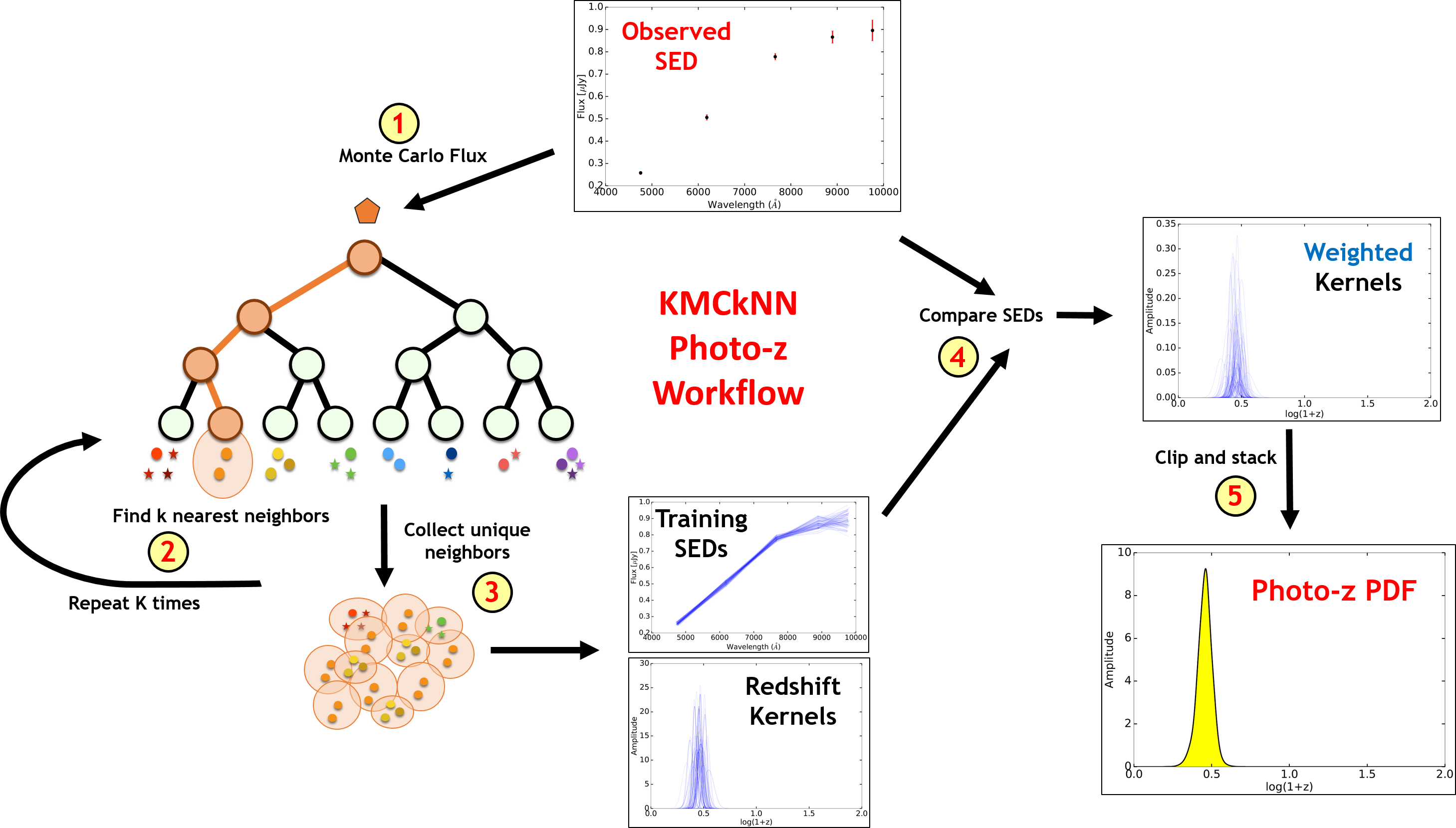
Figure 5: A schematic outline of the major steps in our KMCkNN based algorithm described in §4.3. First, a Monte Carlo realization of the target object indexed by $g$ is matched with a set of $k$ nearest neighbors based on a Monte Carlo realization of all training objects indexed by $h$. After repeating this procedure $K$ times, all unique neighbors in the training set are identified and the corresponding photometric posteriors $P(h|g)$ are computed. These are then used to derive a photo-$z$ PDF based on a posterior-weighted mixture of the corresponding redshift kernels $P(z|h)$.

4.2 Photometric Likelihood

Assuming the errors on the measured fluxes $\mathbf{\hat{F}}_{g}$ and $\mathbf{\hat{F}}_{h}$ are independent and Normal (i.e. Gaussian) and ignoring the impact of selection effects (see, e.g., Leistedt et al. 2016), the log-likelihood for $P(g|h)$ from our set of $B$ bands indexed by $b$ can be naively written as

$$-2\ln P(g|h) =\sum_{b=1}^{B}\frac{\left(\hat{F}_{g,b}-\hat{F}_{h,b}\right)^{2}}{\hat{\sigma}^{2}_{g,b}+\hat{\sigma}^{2}_{h,b}}+\ln(\hat{\sigma}^{2}_{g,b}+\hat{\sigma}^{2}_{h,b})$$ (11)

$$+B\ln 2\pi$$

This represents the standard $\chi^{2}$ statistic often used in template-fitting methods (see §3.1) but with error contributions from both the target ($g$) and training ($h$) objects and including the relevant normalization term.

Unlike most template-fitting codes and contrary to the approach taken in §3, we deliberately chose not to include a free scaling parameter $s$ to try and account for normalization offsets between $g$ and $h$ (i.e. fitting in magnitudes instead of colors). There are two reasons for this. The first is that the conditional prior $P(s|h)$ we would want to impose over $s$ when computing $P(g|h)=\int P(g|h,s)P(s|h)ds$ is unclear. For instance, a fixed prior such as the uniform $P(s|h)=P(s)=1$ prior used by most template-fitting codes is equivalent to assuming a fixed (and unphysical) luminosity function, which can create biases in inference. Trying to specify a color-dependent luminosity function $P(s|h)$ directly, however, is extremely challenging because the integral over $s$ often cannot be evaluated analytically. Fitting flux densities $\mathbf{F}$ directly avoids these complications.

More importantly for our purposes, however, is that our results from §3 show that there can be strong evolution in the underlying redshift distribution $P(z|\mathbf{c},m)$ at fixed color $\mathbf{c}$ as a function of magnitude $m$. To mitigate this effect without attempting to deal with complicated priors, for simplicity we opt to keep the likelihood “close to the data” and fit directly in $\mathbf{F}$.

4.3 Nearest-Neighbors Approximation

To avoid running over all $M$ objects in the training set, we use a modified nearest-neighbors approach to preferentially select objects that have similar flux densities with respect to their errors. As the relative errors $\hat{\bm{\sigma}}^{2}_{g}+\hat{\bm{\sigma}}^{2}_{h}$ of any two training/target objects $g$ and $h$ will differ, the relevant distance metric will be different for every pairwise training-target object combination. As nearest neighbor searches are typically done with respect to a fixed distance metric (often the Euclidean distance), this pairwise distance dependence poses a problem.

We deal with this by using Monte Carlo methods to search for neighbors across multiple realizations of the observed flux densities. We first generate a Monte Carlo realization $\tilde{\mathbf{F}}_{g}$ and $\tilde{\mathbf{F}}_{h}$ of the photometry for all objects in our target set and training set, respectively. We then determine the $k$ nearest neighbors based on the Euclidean squared distance between our set of Monte Carlo-ed flux densities to a given observed galaxy $g$ using a $k$-$d$ tree (Bentley, 1975), defining a set of $k$ indices $\tilde{\mathbf{h}}(g)$. After repeating this process $K$ times, we define an object’s set of “photometric neighbors” as the union of the $k$ nearest neighbors from each of the $K$ Monte Carlo realizations:

$$\tilde{\mathbf{H}}(g)=\tilde{\mathbf{h}}_{1}(g)\cup\cdots\cup\tilde{\mathbf{h}}_{K}(g)$$ (12)

Using our $K$ Monte Carlo $k$ nearest neighbors (KMCkNN) approximation, we only compute photometric likelihoods to a small fraction of the data preferentially selected to contain the highest likelihoods. This procedure is most robust when the set of neighbors is roughly complete out to 3-5 standard deviations (relative to all possible pairwise galaxy combinations). An object can have at most $k\times K$ possible neighbors, with the exact number a strong function of the signal-to-noise of the target object $g$ and the density of training objects $h$ in its local region of color-magnitude space.

The sparse ($kK\ll N_{\mathbf{h}}$) nature of this KMCkNN approximation enables us to keep track of the individual log-likelihoods $\ln P(g|h)$ and their corresponding indices $\tilde{\mathbf{H}}(g)$ across all target objects. Because these have been computed exclusively using observables, we can subsequently use them to construct any associated ancillary quantities “after the fact”. The most relevant example is the photo-$z$ PDFs following equation (10), but this may include a whole range of other useful quantities such as those detailed in §4.5. A schematic diagram of our KMCkNN approach is shown in Figure 5.

One significant drawback of using a nearest-neighbors approach is that it is difficult to accommodate missing data. However, since the weak lensing source catalog used in this work is only defined in regions with full depth and full color coverage (Mandelbaum et al., 2018), this restriction does not impact our results.

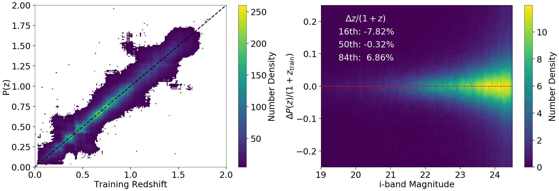
Figure 6: Left: The 2-D stacked distribution of our cross-validation photo-$z$ PDFs as a function of the training redshift for the re-weighted training samples based on the HSC-SSP Wide-depth emulated errors (see §2.3). Right: The reweighted redshift-normalized dispersion $\Delta z/(1+z)$ of our photo-$z$ PDFs relative to the training redshifts as a function of $i$-band magnitude. The 16th, 50th, and 84th percentiles of the marginalized redshift-normalized dispersion for the sample are shown in the upper portion of the figure. Our typical 68%-level uncertainty is $\approx 7.35\%$ with a median bias of $-0.3\%$, illustrating that our photo-$z$ PDFs are robust and unbiased with respect to our training data.

4.4 Photometric Priors

We incorporate the KMCkNN approximation from §4.3 into our photometric prior $P(h)$ by defining a new “sparse” prior

$$\tilde{P}_{g}(h)=\begin{cases}P(h)\quad&\text{for}\>h\in\tilde{\mathbf{H}}(g)\\ 0\quad&\text{otherwise}\end{cases}$$ (13)

Our photo-$z$ PDFs can then be written as

$$P(z|g)\approx\sum_{h\in\tilde{\mathbf{H}}(g)}P(z|h)\frac{P(g|h)P(h)}{P(g)}$$ (14)

Typically, the prior $P(h)$ is defined to adjust for “domain mismatch” between the training and target datasets. Since spec-$z$ training sets are significantly biased in both color and magnitude relative to most target photometric galaxy populations, this “reweighting” via $P(h)$ traditionally substantially improves photo-$z$ accuracy relative to cases where $P(h)$ is assumed to be uniform (Lima et al., 2008).

We compute a photometric “prior” using the magnitude-based, KMCkNN approach described in §4.2 and §4.3 by computing the approximate Bayesian evidence under a uniform prior

$$P(h)\approx\sum_{g\in\tilde{\mathbf{G}}(h)}P(h|g)$$ (15)

where our roles for $g$ and $h$ have switched: we now treat our set of training galaxies indexed by $h$ as “target” objects and a subsample of $N_{\rm ref}$ reference objects indexed by $g$ as “training” objects. We found the impact of the prior on our redshift predictions in internal testing was mostly unchanged for values of $N_{\rm ref}\gtrsim N_{\rm train}$, and so opt to use $N_{\rm ref}=5\times 10^{5}$ here.

To put this procedure another way, we determine $P(h)$ by stacking the likelihoods of neighbors in the target data around individual training objects. This procedure, while not entirely proper (we are using a subset of galaxies in our sample to determine the prior), is sufficient for our purposes and represents the first step to a proper hierarchical model (Leistedt et al., 2016).

We find our prior-weighted training data are able to reproduce the $B$-dimensional distribution of our target data quite well as long as $K$ and $k$ are sufficiently large. See Tanaka et al. (2018) for additional details.

4.5 New Quality Indicators

Unlike other machine learning-oriented approaches, we are able to compute (approximate) posterior quantities to every training-target object pair. This enables us to utilize a variety of Bayesian-oriented indicators to determine the quality of our fits. We will discuss two new quality indicators here: metrics related to basic goodness-of-fit tests (§4.5.1) and those describing the “information content” used in our predictions (§4.5.2).

4.5.1 Goodness-of-Fit

By computing posterior quantities to every pair of training-target objects, we can exploit goodness-of-fit tests used in a broad set of Bayesian model fitting applications. We will examine the two most basic indicators here: the maximum a posteriori (MAP) result $P_{\rm max}(g)\equiv\max\{\dots,P(h|g),\dots\}$ and the evidence $P(g)\equiv\sum_{h\in\mathbf{h}}P(g|h)P(h)$.

The MAP quantifies how good our best-fit result is, enabling us to determine if a given set of observables is represented in our training data. This is extremely useful when trying to remove objects with unreliable predictions that lie outside the parameter space spanned by our training data.

The evidence quantifies how well an object is represented across the entirety of our training data. This is useful when trying to identify objects which do not have meaningful “coverage” since objects that are only similar to a handful of training examples might have unreliable predictions.

In general, we find that the MAP and the evidence are highly correlated among our data: objects that are well-fit by at least one training example are very likely to be well-fit by others, and vice versa. Based on internal testing, we find that instituting a cut explicitly on the best-fit result based on the fitted $\chi^{2}$ values removes the majority of poorly-fit objects from our sample. Our final cut is based on the 95th quantile $P(\chi^{2}_{5}\leq X)=0.95$, where $\chi^{2}_{5}$ is the $\chi^{2}$ distribution with 5 degrees of freedom, which is conceptually roughly equivalent to 2-sigma clipping.

4.5.2 Information Content

As mentioned in §4.3, our sparse KMCkNN approximation allows us to keep track of individual log-likelihoods computed between sets of training-target object pairs. It is then straightforward to transform these results into photo-$z$ PDFs via equation (14).

More generally, however, keeping track of the relevant individual posterior predictions

$$\tilde{P}_{g}(h|g)=\frac{P(g|h)\tilde{P}_{g}(h)}{\sum_{h}P(g|h)\tilde{P}_{g}(h)}$$

allows us to compute almost any posterior-dependent result. This flexibility enables us to investigate auxiliary properties of interest.

In this work, we explore the impact of photo-$z$ systematics on weak lensing using our heterogeneous HSC-SSP training data. In particular, we are worried about the impact many-band photo-$z$’s might have on our results. In order to do this, we introduce two quantities to keep track of where the information content in a given photo-$z$ prediction $P(z|g)$ actually originates:

• Fphot: the fraction of neighbors in the training set with many-band photo-$z$.

• Pphot: the posterior-weighted fraction of neighbors in the training set with many-band photo-$z$.

Fphot and Pphot will help us to determine what kind of redshift (e.g. photo-$z$, spec-$z$, ..) any given object has been trained on. This will be an important ingredient for our lensing tests in Section 7.

5 Photometric Redshift Validation

In this section we outline the implementation (§5.1), validation (§5.2), and application (§5.3) of the photo-$z$ framework outlined in §4.

5.1 Tuning: Feature Selection and (Hyper-)parameter Choices

The HSC-SSP catalog contains a variety of features that can be used for photo-$z$ predictions, including a variety of photometry measurements and size information. In addition, the KMCkNN framework described in §4.3 involves several hyper-parameters that can impact performance.

We conduct a variety of internal cross-validation and hold-out tests following §5.2 to determine the subset of features and hyper-parameters that give the best performance at a reasonable computational cost. Our results are summarized below:

• Our chosen flux density measurements were PSF-matched 1.1$\arcsec$ aperture photometry among objects with successful forced photometry in all five bands. Adding additional features such as size or using different combinations of other photometry products (e.g., cmodel) gave comparable or worse results.

• We introduce a photometric smoothing kernel $\sigma_{g,b}=f_{b}\hat{F}_{g,b}$ for each object $g$ in each band $b$ to account for systematic uncertainties in measured photometric errors and to serve as a smoothing scale when computing likelihoods. We find that $f_{b}=0.02$ gives good photo-$z$ PDFs in aggregate and constitutes an effective zero-point calibration uncertainty of $\approx 0.02\,{\rm mag}$ (although see Tanaka et al. 2018).

• To ensure optimal runtime, we want to make $K$ and $k$ only as large as necessary to obtain good magnitude/color-space coverage for each object. The lower limit on $K$ is set by the number of Monte Carlo realizations needed to roughly marginalize over the measurement uncertainties when searching for neighbors, while the lower limit on $k$ is to ensure a reasonably large collection of neighbors. Based on internal testing, we find $K=25$ Monte Carlo realizations and $k=10$ neighbors selected at each iteration works as a reasonable compromise. The worst case performance ($N_{\rm nghbr}\sim 10$) generally only occurs for bright and rare objects, which usually also have poor likelihoods. The typical number of unique neighbors is $N_{\rm nghbr}\sim 100-200$.

• We take our redshift kernels to be Normal distributions $\mathcal{N}\left({z}\,\middle|\,{\mu=\hat{z}_{h}},{\sigma^{2}=(\Delta z)^{2}+\hat{\sigma}_{h,z}^{2}}\right)$ centered on the measured redshift $\hat{z}_{h}$ with a variance set by a combination of an intrinsic width $\Delta z=0.01$, similar to the redshift spacing used when storing most photo-$z$ PDFs, and the associated redshift measurement error $\hat{\sigma}_{h,z}$. This allows us to propagate uncertainties from the many-band photo-$z$’s to our final predictions.

Following Tanaka et al. (2018), our redshift PDFs $P(z|g)$ are evaluated over a redshift grid ranging from $0\leq z\leq 6$ with $\Delta z=0.01$ spacing. All redshift-based quantities described later in the text are derived from these discretized PDFs.

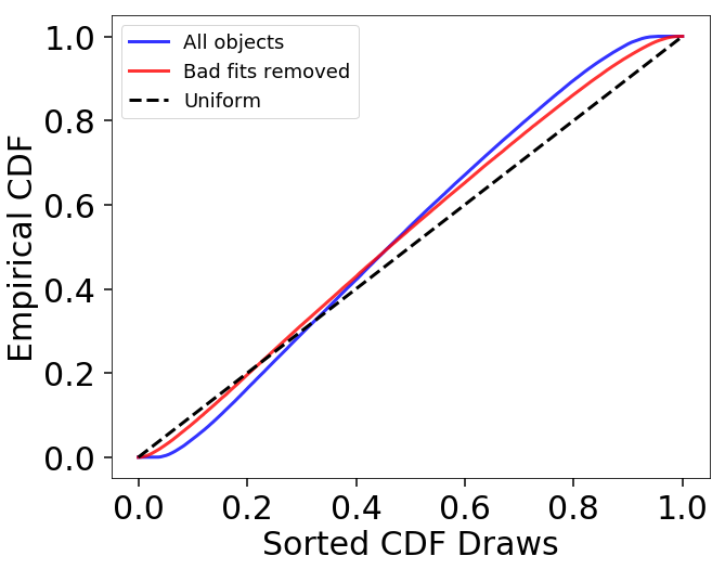
Figure 7: The empirical cumulative distribution function (eCDF) of the “true” redshifts evaluated over the cross-validation photo-$z$ PDFs across the re-weighted training sample before (blue) and after (red) removing “bad” fits ($\sim 5\%$ of the sample) using the criteria outlined in §4.5.1. The ideal behavior is shown as the dashed black line. When limiting to objects that are more represented in our training sample (i.e. have better fits), we are able to remove most outliers with poorly determined PDFs.

5.2 Calibration: Characterizing Behavior with Cross-Validation

As discussed in §2.3, to account for inhomogeneity and domain mismatch in the training set all objects are assigned an HSC-SSP Wide-depth emulated error following the procedure described in Tanaka et al. (2018) and an associated color-magnitude weight following §4.4. Unless stated otherwise, we utilize both quantities when computing any of the performance estimates reported here.

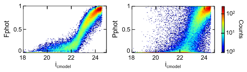
Figure 8: The number density of Fphot (left) and Pphot (right) (see §4.5) as a function of $i$-band magnitude for a representative subsample of $\sim 300$k objects in our HSC-SSP S16A weak lensing sample. As expected, the photo-$z$’s of objects at $i>23$ are trained almost entirely on the many-band photo-$z$’s in our training sample, while those at brighter magnitudes $i<23$ tend to be trained on spec-$z$’s and g/prism-$z$’s. This transition happens more smoothly in Fphot than Pphot because the exponential nature of the likelihood tends to strongly favor a few photometric neighbors over others (see §4.2). This behavior is most apparent at brighter magnitudes, where even though $\sim 15\%$ of neighbors come from many-band photo-$z$’s, they tend to contribute very little to the overall photo-$z$ prediction.

We first randomly divided our training data into validation/hold-out testing sets comprised of $(1-f)$/$f$ fractions of the data for some hold-out fraction $f$. We then use two strategies to select our hyper-parameters and evaluate our performance within the validation set: $k=5$-fold cross-validation and internal leave-one-out tests. For $k=5$-fold cross-validation, we randomly divided our validation set into $k=5$ subsets. We then train on $k-1$ of these subsets to compute photo-$z$ predictions to the remaining subset, cycling through each of the subsets until we had obtained predictions to the entire validation sample. For leave-one-out tests, we instead train on the entire validation set. However, when computing predictions to each object, we “mask out” its possible contribution within the selected group of neighboring objects used to compute the photo-$z$ prediction. Both of these procedures, along with the final hold-out test set, attempt to mitigate over-fitting and ensure realistic performance estimates.

We find that the results from §5.1 are mostly insensitive to the chosen hold-out fraction $f$ when $f\gtrsim 0.5$ (i.e. when our validation set consists of more than $\sim$ 150k objects). In addition, we also find that the performance on the hold-out test set is essentially identical to performance estimates within the validation set using both strategies when $f\gtrsim 0.8$, confirming that our approaches avoid over-fitting and that the information content appears to roughly saturate as our validation set exceeds $\sim$ 250k objects. Based on these results, we find that it is reasonable to treat our features and hyper-parameters from §5.1 as essentially fixed. Our reported performance is then estimated by applying the more conservative $k=5$-fold cross-validation tests across the entire training sample (i.e. without the $(1-f)/f$ validation/testing split).

The 2-D stacked photo-$z$ PDFs versus the input true redshifts (smoothed by their intrinsic uncertainties) along with the associated dispersion in $\Delta z/(1+z)$ as a function of magnitude are shown in Figure 6. We see that our performance over the weak lensing sample is relatively robust, with an overall $\Delta z/(1+z)\approx-0.3\%$ bias and with 68% of the PDFs contained within $\Delta z/(1+z)=[-7.8\%,6.9\%]$.

In addition to tests on the overall accuracy of our predictions, we also test the reliability of our individual PDFs. We opt to use the empirical cumulative distribution function (eCDF), which is constructed by evaluating the true redshift of each cross-validation object $i\in\mathbf{i}$ at the value of the predicted photo-$z$ CDF

$$\hat{u}_{i}\equiv\int_{0}^{z_{i}}P(z|i)dz$$ (16)

and computing

$$\hat{U}(x)=\sum_{i}\mathbb{I}(\hat{u}_{i}\leq x)$$ (17)

where $\mathbb{I}(\cdot)$ is the indicator function which returns $1$ if the condition is true and $0$ if it is false. In the case where our PDFs are properly calibrated and have the expected coverage provided by any associated confidence interval, each CDF draw $\hat{u}_{i}\sim\textrm{Unif}(0,1)$ will be uniformly distributed from 0 to 1 and $\hat{U}(x)$ will approximately define a straight line from 0 to 1.

We show the eCDF results for our photo-$z$ PDFs in Figure 7. These confirm that our PDFs are relatively robust and internally well-calibrated.

5.3 Application: Estimating Spectroscopic Incompleteness

We now turn our attention to the motivating issue behind the development of the photo-$z$ framework outlined in §4 by investigating the distribution of Fphot and Pphot (see §4.5.2) within our HSC-SSP photo-$z$’s.

We show the distribution of Fphot and Pphot as a function of magnitude in Figure 8. The results are as expected: many-band photo-$z$’s in our training sample make up an increasing large fraction of neighbors and contribute an increasing amount to the photo-$z$ PDFs at fainter magnitudes. We will use Fphot and Pphot to investigate the robustness of weak lensing measurements as a function of spectroscopic incompleteness (see §7).

6 Lensing Methodology

We now outline the methodology we will use to stack, compute, and compare our gg lensing signals based on the photo-$z$ PDFs illustrated in §5. We describe our basic computation of $\Delta\Sigma$ in §6.1 and our treatment of the bias/dilution factors in §6.2. We outline the approach used to compare gg lensing signals between two samples in §6.3.

6.1 Computing the Galaxy-Galaxy Lensing Signal

Our computation of the lensing observable, $\Delta\Sigma$, follows the methodology of Singh et al. (2017). We use the code dsigma, which was specifically written for computing gg lensing signals for HSC-SSP.

We compute $\Delta\Sigma$ as a function of physical radius $R$ as

$${\Delta\Sigma}_{\rm LR}(R)=f_{\rm bias}({\Delta\Sigma}_{\mathrm{L}}(R)-{\Delta\Sigma}_{\mathrm{R}}(R))$$ (18)

where ${\Delta\Sigma}_{\mathrm{L}}$ is the stacked signal around lens galaxies, ${\Delta\Sigma}_{\mathrm{R}}$ is the stacked profile around a much larger number of random positions, and $f_{\rm bias}$ is a correction factor (see §6.2). The ${\Delta\Sigma}$ profile for both lenses and randoms are computed as follows:

$${\Delta\Sigma}_{L}(R)=\frac{1}{2R(R)[1+K(R)]}\frac{\Sigma_{\rm Ls}^{R}w_{\rm Ls}\gamma_{t}^{(\rm Ls)}\Sigma_{\rm crit}^{(\rm Ls)}}{\Sigma_{\rm Ls}^{R}w_{\rm Ls}}$$ (19)

where $\sum_{\rm Ls}^{R}$ indicates a sum over all lens-source pairs with separation $R$. When computing ${\Delta\Sigma}_{R}(R)$, we replace $\sum_{\rm Ls}^{R}$ with $\sum_{\rm Rs}^{R}$ since we instead sum over all random-source pairs.

In Equation 19, $\gamma_{t}$ is the tangential shear of a source galaxy:

$$\gamma_{\rm t}=-e_{1}\cos{2\phi}-e_{2}\sin{2\phi}$$ (20)

where $e_{1}$, $e_{2}$, and $\phi$ are the two shear components and the angle from the direction of right ascension to the lens-source direction in sky coordinates measured by the HSC-SSP pipeline (Mandelbaum, 2018; Bosch et al., 2018). $\Sigma_{\rm crit}$ is the critical surface mass density:

$$\Sigma_{\rm crit}=\frac{c^{2}}{4\pi G}\frac{D_{\rm A}(z_{\rm s})}{D_{\rm A}(z_{\rm L})D_{\rm A}(z_{\rm L},z_{\rm s})}$$ (21)

which is computed using the angular diameter distance between the source and observer $D_{\rm A}(z_{\rm s})$, lens and observer $D_{\rm A}(z_{\rm l})$, and source and lens $D_{\rm A}(z_{\rm L},z_{\rm s})$. Each source galaxy is weighted by:

$$w_{\rm Ls}=\frac{\Sigma_{\rm crit}^{-2}}{\sigma^{2}_{e,{\rm Ls}}+\sigma^{2}_{\rm rms}}\equiv\frac{\Sigma_{\rm crit}^{-2}}{\sigma^{2}_{{\rm Ls}}}$$ (22)

where $\sigma_{\rm rms}$ is the intrinsic shape dispersion per component and $\sigma_{e,Ls}$ is the per-component shape measurement error (see Mandelbaum et al., 2018). $\mathcal{R}(R)$ is the shear responsivity factor that describes the response of galaxy ellipticity to a small amount of shear:

$$\mathcal{R}(R)=1-\frac{\Sigma_{\rm Ls}^{R}w_{\rm Ls}\sigma^{2}_{{\rm Ls}}}{\Sigma_{\rm Ls}^{R}w_{\rm Ls}}$$ (23)

We compute and apply $\mathcal{R}$ independently for each radial bin.

The $[1+K(R)]$ term is a correction for the multiplicative shear bias $m$:

$$K(R)=\frac{\Sigma_{\rm Ls}^{R}w_{\rm Ls}m_{\rm s}}{\Sigma_{\rm Ls}^{R}w_{\rm Ls}}$$ (24)

where $m_{\rm s}$ is a per source value that is calibrated using simulations. Please see Mandelbaum et al. (2018) for details about the calibration of HSC-SSP weak lensing catalog.

In this work, we use $10^{5}$ random points to compute ${\Delta\Sigma}_{\rm R}$ sampled following the HSC-SSP S16A survey geometry. Random points are assigned redshifts following the redshift distribution of lenses. Although Singh et al. (2017) use the boost factor ($\Sigma_{\rm Ls}^{R}w_{\rm Ls}/\Sigma_{\rm Rs}^{R}w_{\rm Rs}$) to correct for dilution effects (see also Mandelbaum et al. 2005), we do not apply any boost factor corrections here. Instead, in Section 7.4 we test whether or not the signal varies as we impose more stringent lens-source separation cuts.

We assume physical coordinates and compute $\Delta\Sigma$ in 10 logarithmically spaced bins from 0.05 Mpc to 15 Mpc. Errors on all $\Delta\Sigma$-related quantities are computed via bootstrap resampling. The dsigma code divides lenses and randoms to roughly equal-area regions. Here we use 40 regions with typical sizes of $\sim$ 2.5 deg and compute errors with $N_{\rm Bs}=5000$ bootstraps.

6.2 Corrections for Photometric Redshift Bias and Dilution Factors

Our procedure for estimating the bias on $\Delta\Sigma$ arising from photo-$z$’s partially follows that of Mandelbaum et al. (2008), Nakajima et al. (2012), and Leauthaud et al. (2017). We summarize our approach here.

To correct for biases in $\Delta\Sigma$ arising from photo-$z$ errors, a common procedure is to use set of galaxies with spectroscopic redshifts that have been re-weighted with appropriate color-magnitude weights (see §4.4) to match the source distribution. However, as shown in Figures 2 and 8, the currently available spec-$z$’s in our training set are so underrepresented in some regions of color-magnitude space that it is impossible to properly re-weight them (spec-$z$’s) to match the source sample.

For this reason, instead of a spectroscopic redshift catalog, we build a calibration catalog based on the set of many-band photo-$z$’s in the COSMOS field matched with observations taken at HSC-SSP Wide depths with weak lensing cuts applied (see §2.2). Our assumption here is that the COSMOS many-band photo-$z$’s have narrow enough PDFs that they can be used to compute biases on $\Delta\Sigma$ for HSC. We refer to this catalog hereafter as the COSMOS calibration sample.

We compute the bias on $\Delta\Sigma$ as follows. Let $\Delta\Sigma_{\rm P}$ ($\Sigma_{\mathrm{crit,P}}$) represent the value of $\Delta\Sigma$ measured with photo-$z$’s and $\Delta\Sigma_{\rm T}$ ($\Sigma_{\mathrm{crit,T}}$) represent the true value of $\Delta\Sigma$. We define $f_{\rm bias}\equiv\Delta\Sigma_{\rm T}/\Delta\Sigma_{\rm P}$ and estimate it via:

$$f_{\rm bias}=\frac{\sum_{\rm Ls}w_{\rm Ls}\left(\Sigma_{{\rm crit,T,Ls}}/\Sigma_{{\rm crit,P,Ls}}\right)}{\sum_{\rm Ls}w_{\rm Ls}}$$ (25)

where the sum is performed over source galaxies drawn from the COSMOS calibration sample. Unlike other versions of this equation (e.g. Equation A3 in Leauthaud et al. 2017) there is no re-weighting factor to account for color mis-matches between the source sample and the calibration sample because our COSMOS calibration sample is already representative.

For a given lens sample, we estimate $f_{\rm bias}$ using Monte Carlo methods by randomly drawing sources from our COSMOS calibration catalog and lens redshifts from the lens sample. We correct all $\Delta\Sigma$ values reported hereafter using $f_{\rm bias}$. This accounts for the dilution effect by sources that scatter above $z_{\rm L}$ but which are actually located at redshifts below $z_{\rm L}$).

More explicitly, there are three issues: the impact of photo-$z$ scatter and bias for sources that are above the lens redshift, dilution due to sources that are below the lens redshift but get scattered above it due to photo-$z$ error, and dilution due to physically-associated sources. Our approach corrects for the first two of these, but not the third.

For our signals, typical values for $f_{\rm bias}$ are around a few percent ($\sim 2-5\%$).

6.3 Comparing Lensing Signals

One of the primary concerns in this work is the robustness of the gg lensing signal with respect to possible photo-$z$ biases. Since an absolute calibration does not exist, we instead aim to demonstrate the robustness of the signal to various cuts and choices for lens-source separation. We quantify this by considering the ratio of $\Delta\Sigma$ for two different computations $i$ and $j$:

$$f_{i,j}\equiv\Delta\Sigma_{i}/\Delta\Sigma_{j}.$$ (26)

This ratio test assumes that when we change how we calculate the gg lensing signals (by, e.g., tweaking the source sample selection or the redshift estimator), the true $\Delta\Sigma(R)$ should be the same (i.e. $\Delta\Sigma_{i}(R)=\Delta\Sigma_{j}(R)$ for all $R$). This relies on the assumption that $\Delta\Sigma(R)$ does not vary much across the sample within the lens redshift bins. In other words, we assume that changing the source sample in a way that emphasizes different redshifts within the lens sample does not meaningfully change $\Delta\Sigma(R)$ given the same photo-$z$ quality across both source samples.

While it is straightforward to take the ratio between two lensing signals with different source cuts, ${\Delta\Sigma}_{i}$ and ${\Delta\Sigma}_{j}$ will be highly correlated. To deal with this effect, we derive the covariance matrix for $f$ via bootstrap resampling using the same bootstrap regions as described previously.

We assume that $f_{i,j}$ is a constant (we only consider amplitude changes) and solve for the maximum-likelihood result (MLE). We fit for amplitude shifts over our full radial range (denoted $f_{\rm all}$) and also over the radial range $R=[0.1,1]$ Mpc (denoted $f_{\rm inner}$) and $R=[1,10]$ Mpc (denoted $f_{\rm outer}$).

7 Results: How Robust is the Galaxy-Galaxy Lensing Signal?

We now investigate how robust gg lensing signals are to various photo-$z$ estimators and quality cuts. After exploring changes in the gg lensing sensitivity to a variety of choices (§7.2-§7.6), we subsequently use the results of those choices to define a “fiducial” sample (see §7.7). Our results are presented in terms of the stability of the gg lensing signal based on other possible choices with respect to our fiducial sample.

The various cuts that we test comprise 15 unique lens-source samples. These are described in detail below and summarized in Table 1.

Since we perform a large number of tests ($3\times 3\times 14=126$) in the subsequent sections, many often correlated, we might expect by pure statistical chance that some of the results reported might have deviated from the expected null result by a large amount. We attempt to control against these in two ways. First, since for each lens sample we compute $f_{\rm all}$, $f_{\rm inner}$, and $f_{\rm outer}$ under 14 configurations, we expect at most one test to display outliers at $>3\sigma$ significance. We thus adopt a $3\sigma$ threshold as reasonably indicative of a significant deviation. In addition, we also compare the distribution of our error-normalized $f/\sigma_{f}$ values to those expected under a Gaussian distribution using a Kolmogorov-Smirnov (KS) test. While the sample size is small, we find that for all cases our results are inconsistent with a Gaussian distribution, with the results driven primarily by outliers.

Table 1: Redshift estimates and selection criteria used to construct robustness tests for galaxy-galaxy lensing. V indicates that the quantity is varied for a particular test, while F indicates that it is kept fixed. These comprise a total of 15 unique lens-source samples.

Test	§7.2	§7.3	§7.4	§7.5	§7.6
Photo-z Estimate
Mean	V
Median	V
Mode	V
Best	V	F	F	F	F
MC	V
Photo-z Quality Cut
basic		V
medium	F	V	F	F	F
strict		V
Lens-Source Separation
$z_{\rm{low68}}>z_{\rm lens}+0.1$			V
$z_{\rm{low68}}>z_{\rm lens}+0.2$			V
$z_{\rm{low95}}>z_{\rm lens}+0.1$	F	F	V	F	F
$z_{\rm{low95}}>z_{\rm lens}+0.2$			V
High/Low Redshift
All	F	F	F
zlow				V
zhigh				V	F
photo-$z$ Origin
All	F	F	F	F
plow					V
pmed					V
phigh					V

7.1 Lens Sample

We use all galaxies with spectroscopic redshifts (both the LOW-Z and CMASS samples) from the Sloan Digital Sky Survey (SDSS) II and III Baryon Acoustic Oscillation Survey (BOSS) (Abazajian et al., 2009; Eisenstein et al., 2005) that overlap with the HSC-SSP survey footprint. We apply the same geometric masks to the lens sample that were used when constructing the source sample (see §2.2).

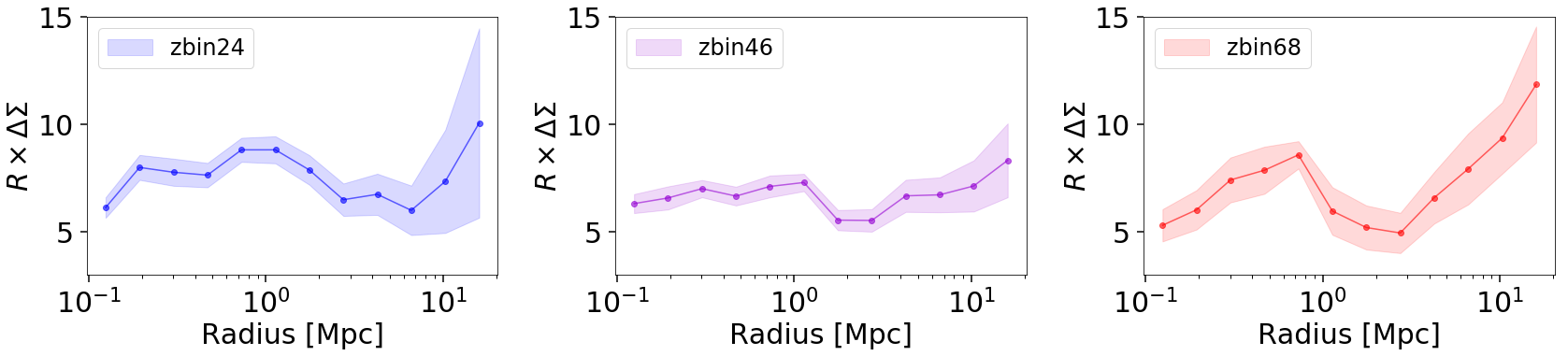
Figure 9: $\Delta\Sigma(R)$ signals computed for our fiducial sample (defined in §7.7) from BOSS CMASS and LOWZ lenses from $0.2<z_{\rm lens}\leq 0.4$ (left, blue), $0.4<z_{\rm lens}\leq 0.6$ (middle, purple), and $0.6<z_{\rm lens}\leq 0.8$ (right, red). The mean values are highlighted as solid lines and points, while the shaded region encompasses the 1-$\sigma$ errors.

To explore the stability of the lensing signal as a function of redshift, we group the lens population into three separate redshift bins:

• zbin24: $0.2<z<0.4$

• zbin46: $0.4<z<0.6$

• zbin68: $0.6<z<0.8$

They contain $\approx$ 4000, 12000, and 4000 lenses, respectively. All the tests described below and summarized in Table 1 were computed for each redshift bin, leading to a total of 45 $\Delta\Sigma(R)$ measurements. The gg lensing signal for our fiducial sample (see §7.7) in each redshift bin is shown in Figure 9.

7.2 Photometric Redshift Point Estimates

In lensing analyses, $\Delta\Sigma$ is often computed with respect to fixed point estimates derived from the photo-$z$ PDFs to avoid having to integrate over all photo-$z$ PDFs $P(z|g)$’s.

We study whether or not the particular choice of a point source estimate impacts the gg lensing signal. We compare five point estimates in this paper:

• $z_{\rm mean}$, the first moment (mean) of the photo-$z$ PDF,

• $z_{\rm med}$, the 50th percentile (median) of the photo-$z$ PDF,

• $z_{\rm mode}$, the redshift corresponding to the maximum value of the photo-$z$ PDF,

• $z_{\rm best}$, the redshift estimator that minimizes the loss assuming a Lorentzian kernel in $\Delta z/(1+z)$ with a width of $\sigma=0.15$ (see Tanaka et al. 2018 for additional details), and

• $z_{\rm mc}$, a Monte Carlo draw from the photo-$z$ PDF.

A comparison with integrating over the PDF is beyond the scope of this work and is discussed further in More et al. (in prep.).

Most of these point estimates have been used to varying degrees in weak lensing analyses in the literature, each with various benefits and drawbacks. Here we will briefly outline the arguments for each estimator (see also Tanaka et al. 2018).

While beyond the scope of this paper, it is well known that the mean estimate $z_{\rm mean}$ is the optimal point estimate for a PDF assuming “squared error” ($L_{2}$) loss. In other words, if we introduce a penalty proportional to $(z_{\rm est}-z_{\rm true})^{2}$ and assume $z_{\rm true}$ follows our PDF, then $z_{\rm est}=z_{\rm mean}$ is the estimator that is “best” given the PDF. This particular result is optimal for Gaussian distributions.

In general, however, most photo-$z$ PDFs are not Gaussian, but instead can have asymmetric tails and/or extended shapes. The mean $z_{\rm mean}$ is particularly sensitive to these tails, and so estimates that are more “robust” are sometimes preferred. As with the mean, it can likewise be shown that the median $z_{\rm med}$ is the optimal point estimate under “absolute” ($L_{1}$) loss where the penalty is proportional to $|z_{\rm est}-z_{\rm true}|$. This reduced penalty makes $z_{\rm med}$ less sensitive to the tails. The mode $z_{\rm mode}$ can likewise be shown to be the optimal point estimate under “unforgiving” loss ($L_{0}$) where the penalty is maximized and constant for all $z_{\rm est}\neq z_{\rm true}$. This penalty makes $z_{\rm mode}$ only sensitive to the peak of the PDF where the probability is maximized.

While these various estimators are optimal under different assumptions for how much we want to penalize “incorrect” guesses, none of them are specifically tuned for photo-$z$ estimation. In particular, most PDFs and photo-$z$ applications tend to have a dependence on $|z_{\rm est}-z_{\rm true}|/(1+z_{\rm true})$ rather than just $|z_{\rm est}-z_{\rm true}|$, and also care about being accurate relative to a given “tolerance” $\sigma$. $z_{\rm best}$ is the point estimate that minimizes the loss relative to these conditions.

Finally, we may want a point estimate that “explores” the entire PDF, rather than attempting to “summarize” it. Assuming “uniform” loss (i.e. a flat penalty everywhere), any Monte Carlo sample $z_{\rm mc}$ from the PDF serves as a reasonable point estimate. These may better capture the behavior of PDFs by allowing us to probe, e.g., the tails of the distribution but lead to some (additional) amount of random noise being introduced.

The $\Delta\Sigma$ ratio estimates computed based on each of these various redshift point estimates with respect to our fiducial sample in each redshift bin are shown in the top two rows of Figures 10, 11, and 12. We find that, with the exception of $z_{\rm mc}$, all of these choices result in negligible ($\lesssim 1\%$), albeit sometimes statistically significant (at 3$\sigma$), differences in the computed $\Delta\Sigma$. This is likely due to the general quality of our PDFs, which are reasonably well-constrained and unimodal for the majority of objects (see Figure 6) and also well-calibrated against the expected underlying redshift distribution (Figure 7), leading to very similar point estimates.

In general, using Monte Carlo redshifts $z_{\rm mc}$ tends to lead to an underestimate of the $\Delta\Sigma$ signal by an increasing amount as a function of the lens redshift. This is due to the (exponentially) increasing sensitivity of the $\Delta\Sigma$ signal at close lens-source separations as well as increasing photo-$z$ uncertainties at higher redshifts. Since Monte Carlo redshifts scatter sources around based on their PDFs, these tend to dilute the computed signals relative to the more “stable” point estimates above.

Since there is no (relevant) statistical difference between the photo-$z$ point estimates excluding $z_{\rm mc}$, we decide to use the $z_{\rm best}$ estimate due to its superior performance relative to the other estimators when predicting redshifts for individual objects within the full HSC-SSP S16A Wide sample. For additional comparisons between the per-object accuracy of these photo-$z$ point estimates, see Tanaka et al. (2018).

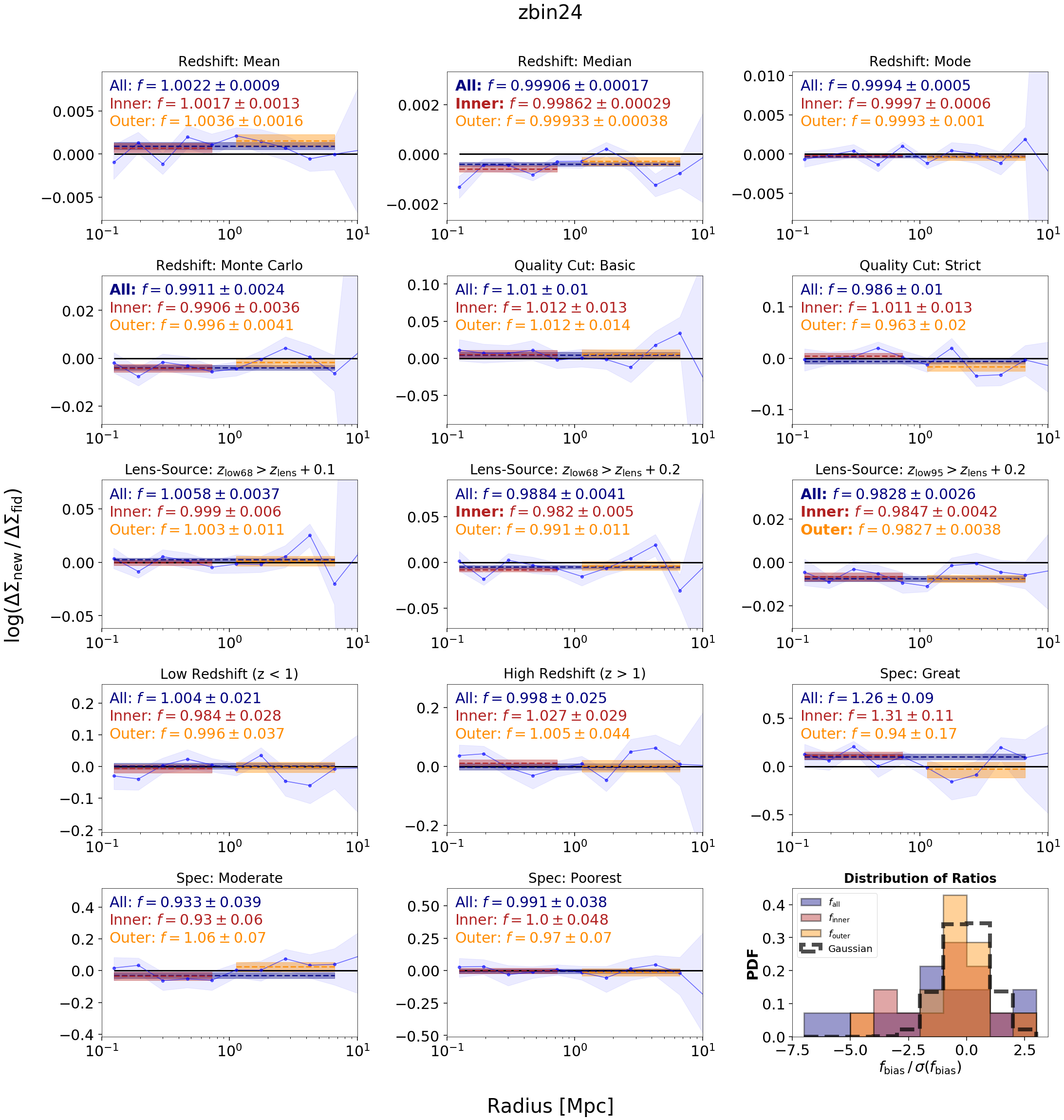
Figure 10: Bootstrap ratios $f_{\rm new,\,fid}$ between new $\Delta\Sigma_{\rm new}(R)$ signals computed using the zbin24 lens sample ($0.2<z_{\rm lens}\leq 0.4$) relative to our fiducial sample $\Delta\Sigma_{\rm fid}(R)$. The null result ($f=1$) is shown as a solid black line, while the maximum-likelihood estimator for $f_{\rm all}$ (dark blue) and $f_{\rm inner}$ and $f_{\rm outer}$ (dark red) for each sample are shown as dotted lines and listed in the upper-left-hand corner of each plot. 1-$\sigma$ errors on all quantities are shown as shaded regions. A 1-D histogram of the error-normalized distribution of $f$, $f_{\rm inner}$, and $f_{\rm outer}$ is displayed in the bottom-right corner along with a Gaussian distribution for reference. Most of the computed ratios are consistent with the expected null result at 3$\sigma$; those that disagree are highlighted in bold. Although these disagreements are statistically significant, some (e.g., with respect to $z_{\rm med}$) are negligible in practice since their impact is $\lesssim 1\%$. In general, $f_{\rm outer}$ is more unbiased for all samples than $f$ and $f_{\rm inner}$. See §7 for additional discussion and details.

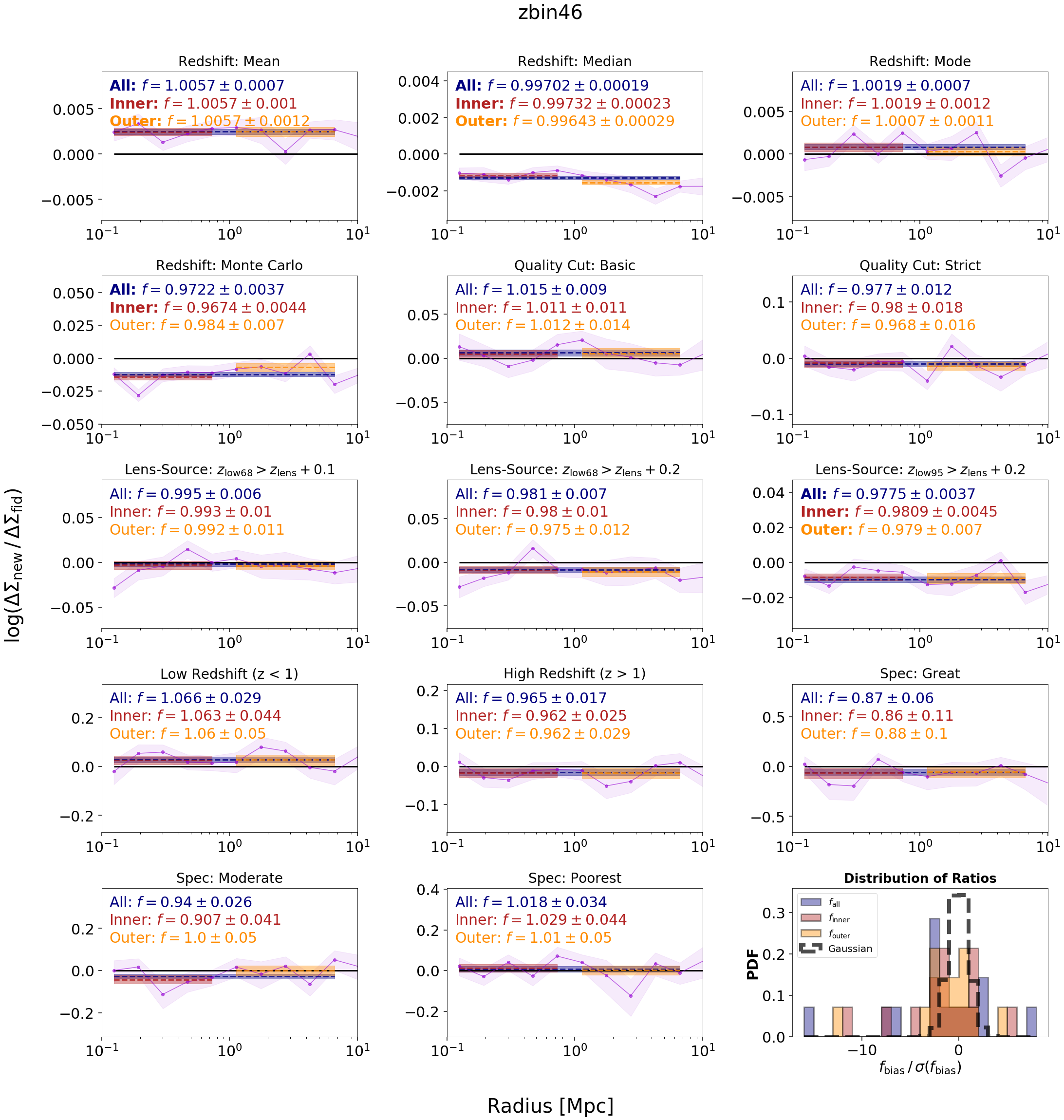
Figure 11: As Figure 10, but for zbin46 ($0.4<z_{\rm lens}\leq 0.6$).

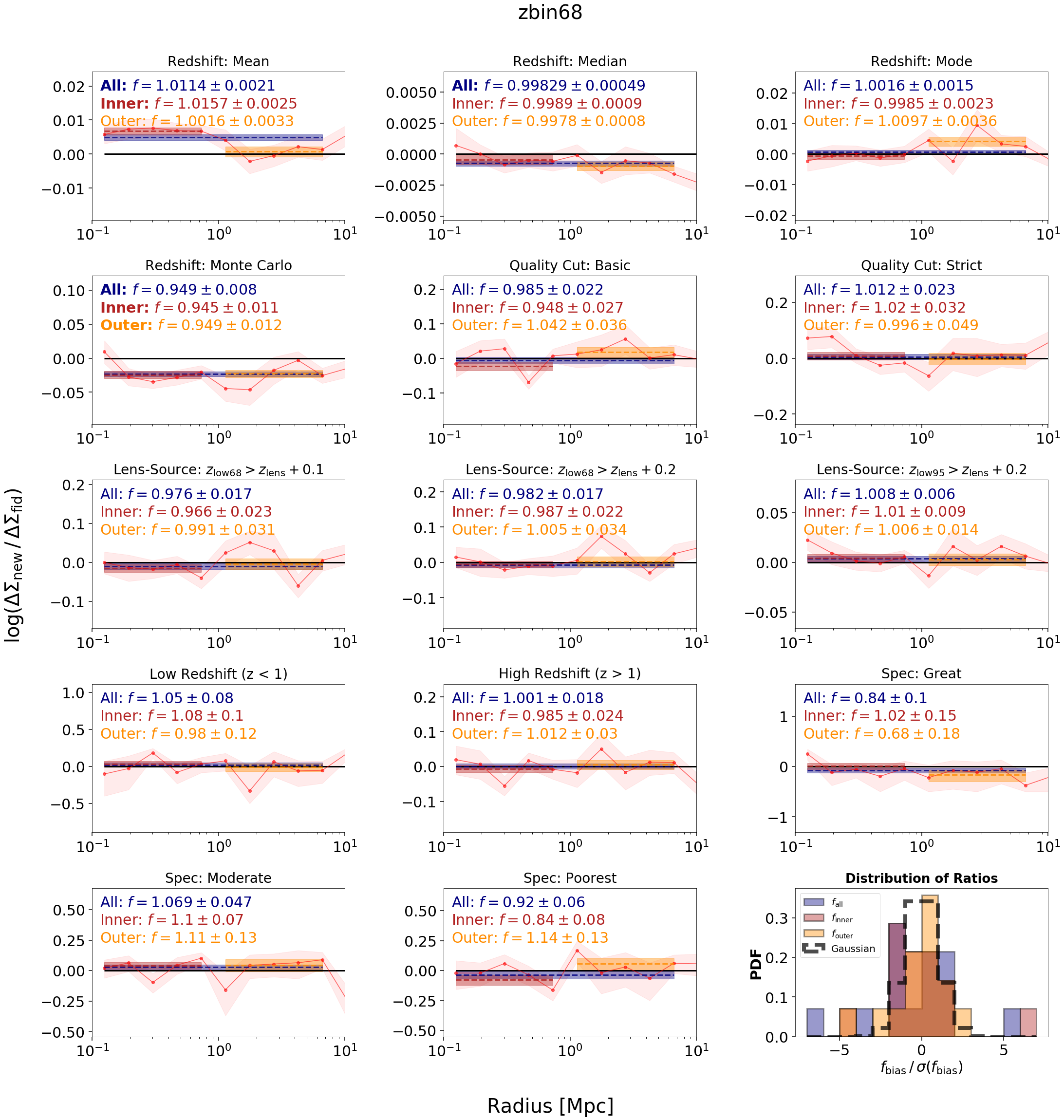
Figure 12: As Figure 10, but for zbin68 ($0.6<z_{\rm lens}\leq 0.8$).

7.3 Photometric Redshift Uncertainties

Although our photo-$z$ PDFs are well-calibrated with respect to the underlying redshift distribution (§5.2), in general using point estimates to summarize broad PDFs can lead to distortions in the underlying redshift population (Carrasco Kind & Brunner, 2014b). In addition, broad photo-$z$ PDFs where the probability density spans a large redshift range are generally seen as more unreliable, with more potential for miscalibrations that can lead to under/overestimated uncertainties on the prediction compared to narrower PDFs. As a result, it is common in many gg lensing analyses to remove “unreliable” photo-$z$’s based on the width of their PDFs.

We define two main sources of uncertainty that contribute to unreliable PDFs. The first is systemic uncertainty: having a poor understanding of the object in question and therefore an unreliable redshift prediction. This can occur if the object is not well-represented within the training set, which leads to them having large $\chi^{2}$ values when comparing to their closest color-magnitude neighbors. We can exploit this fact to flag and remove these sources explicitly.

The second source of uncertainty is statistical uncertainty: utilizing a point estimate that does not accurately represent the PDF. This can occur if the redshift PDF is overly broad or multi-modal with several possible redshift solutions. We quantify this source of uncertainty by defining the “risk” (Tanaka et al., 2018) that the point estimate is incorrect is the integral over the PDF with respect to the associated loss

$$R(z_{\rm phot})=\int P(z)L(z,z_{\rm phot})\,dz$$ (27)

where the particular loss function

$$L(z,z_{\rm phot})=1-\frac{1}{1+\left(\frac{z_{\rm phot}-z}{\gamma(1+z)}\right)^{2}}$$ (28)

is taken to be a Lorentzian kernel with a width of $\gamma=0.15$. The best redshift estimate and the associated risk $z_{\rm risk}$ are then defined jointly as

$$z_{\rm risk}=\min\{R(z)\}=R(z_{\rm best}$$ (29)

Sources with higher $z_{\rm risk}$ generally have broader PDFs with multiple peaks. See Tanaka et al. (2018) for additional discussion.

We divide our sample into a number of sub-samples based on a range of photo-$z$ quality cuts. These are:

• basic: $\chi^{2}_{5}\leq 6$. This is the $\chi^{2}_{5}$ value corresponding to the 95% cut discussed in §4.5 since $P(\chi^{2}_{5}\leq 6)\approx 0.95$ for a chi-square distributed random variable with 5 degrees of freedom. As expected, this removes $\sim 5\%$ of sources. The majority of these sources are at brighter magnitudes and lower redshifts and do not not contribute significantly to the gg lensing signal.

• medium: In addition to basic, this selection also imposes a cut on the “risk” of a particular photo-$z$ point estimate $z_{\rm risk}<0.25$. This generally removes overly broad PDFs and leaves $\sim 75\%$ of the sample.

• strict: In addition to basic, this selection imposes a stricter cut of $z_{\rm risk}<0.15$, restricting our estimates to even narrower PDFs than medium. This leaves $\sim 60\%$ of the sample.

The $\Delta\Sigma$ ratio estimates computed for each of these global photo-$z$ quality cuts with respect to our fiducial sample are shown in the second row of Figures 10, 11, and 12. We find that the computed $\Delta\Sigma$ signals appear insensitive to the global photo-$z$ quality cut chosen, and are statistically consistent with the null result (at 3$\sigma$). As with §7.2, this is likely due to the fact that our PDFs are both relatively well-constrained and well-calibrated for the majority of our sample, especially since any outlying PDFs are removed by our initial basic quality cuts.

Since our performance is similar across different global photo-$z$ quality cuts, we opt to use our medium cut for our fiducial sample to compromise between sample size and PDF quality.

7.4 Lens-Source Separation

In addition to possible biases based on how the photo-$z$ point estimates trace the underlying source population, it is also imperative to ensure that any possible differences we observe are not dominated by dilution effects or contamination from correlated objects (see §6.2). This is often done by imposing cuts that aim to ensure that the bulk of any source galaxy PDF lies behind the lens population (e.g., Medezinski et al. 2018; see also §7.2).

We parameterize this cut using two parameters. The first is a summary statistic detailing the redshift below which X% ($z_{\rm{lowX}}$) of the source galaxy PDF lies, which we use to establish how confidently we can place a source galaxy behind a given lens. In other words, X% of the photo-$z$ PDF is above a redshift of $z_{\rm{lowX}}$, which should be greater than the redshift of the lens $z_{\rm lens}$. The second is a “buffer” $\Delta z_{\rm lens}$ to establish a minimum separation threshold between the source $z_{\rm lowX}$ and the lens $z_{\rm lens}$. This term is used to avoid being extremely sensitive to photo-$z$ biases and possible miscalibrations in the corresponding PDFs since the dependence of $\Sigma_{\rm crit}$ is highly non-linear when $z_{\rm source}$ and $z_{\rm lens}$ are very close together.

We test four lens-source separation cuts:

• $z_{\rm{low68}}>z_{\rm lens}+0.1$

• $z_{\rm{low68}}>z_{\rm lens}+0.2$

• $z_{\rm{low95}}>z_{\rm lens}+0.1$

• $z_{\rm{low95}}>z_{\rm lens}+0.2$

for $X=68\%$ and 95% (roughly 1 and 2-sigma) and $\Delta z_{\rm lens}=0.1$ and 0.2, listed roughly in order from most aggressive to most conservative.

Our results are shown in the third and fourth rows of Figures 10, 11, and 12. We find that all cases are consistent (at 3$\sigma$) with the null result with the exception of the $z_{\rm{low95}}+0.2>z_{\rm lens}$ cut for the zbin24 lens sample, which is smaller by $\approx 1.5\%$. As the most conservative cut in the lowest redshift bin (which should be least-sensitive to photo-$z$ issues), it is somewhat surprising that we see a noticeable suppression. While it is possible that this is just statistical noise, it might also be the case that the photo-$z$’s in the training set have systematic discrepancies at intermediate redshifts that are accentuated when only the low-$z$ sources are removed.

In general, however, these results support the gg lensing signal being mostly insensitive to these specific combination of lens-source separation cuts for our HSC-SSP S16A data. This implies that the majority of our sources are correctly selected to be behind the bulk of the lens sample, providing additional (indirect) support that our photo-$z$ PDFs are well-calibrated. These results also suggest that our gg lensing signals do not require any boost factor corrections.

Given that these lens-source separation cuts perform comparably, we again opt to use a compromise for our fiducial sample by choosing $X=95\%$ and $\Delta z_{\rm lens}=0.1$.

7.5 High and Low Redshift Sources

One additional concern is our gg lensing analysis may be sensitive to degrading photo-$z$ quality as a function of redshift. This is in general due to a combination of spectroscopic incompleteness at higher redshifts and fainter magnitudes as well as broader PDFs arising from noisier photometry (see §3). This is a particularly acute concern for this work due to our reliance on many-band photo-$z$’s at the magnitudes and redshifts probed by a significant majority of our weak lensing source galaxies.

To investigate this effect, we divide our source sample into high-redshift and low-redshift samples to investigate this effect defined by:

• zlow: $z_{\rm best}\leq 1$, which leaves $\sim 50\%$ of the sample.

• zhigh: $z_{\rm best}>1$, which leaves $\sim 50\%$ of the sample.

The results for our high and low-redshift samples are shown in the fourth row of Figures 10, 11, and 12. Although we find the $\Delta\Sigma$ signals from zlow to be systematically higher than those from zhigh, the effect is not statistically significant and both agree with the null result (at 3$\sigma$). This provides us with confidence that we can utilize photo-$z$’s for source galaxies at all redshifts when constructing our fiducial sample.

7.6 Origin of Training Redshifts

One benefit of the KMCkNN framework outlined in §4 is that we actually have a direct proxy of spectroscopic incompleteness through metrics such as Fphot and Pphot, in addition to indirect proxies such as the high/low redshift split used in §7.5. This allows us to examine how robust our gg lensing signals are depending on the information content used to estimate the photo-$z$’s of individual source galaxies.

One complication of using Pphot to select source galaxies directly is that it tends to be strongly correlated with magnitude and redshift, with sources with lower redshifts and brighter magnitudes tending to also have lower Pphot. We attempt to alleviate this issue by limiting our analysis to the zhigh subset of galaxies ($z_{\rm best}>1$). While this substantially reduces the sample (by 50%), it mitigates some of the extreme differences that can arise due to these effects.

As a compromise between preserving number density and maximizing differences between sources that are many-band photo-$z$-dominated versus those that are not, we ultimately split our source galaxies into three subsamples based on spec-$z$ and g/prism-$z$ information content:

• “Great”: $\texttt{Pphot}<0.5$ (i.e. $>50\%$ of information comes from spec-$z$’s and g/prism-$z$’s), which leaves $\sim 10\%$ of the sample.

• “Moderate”: $0.5\leq\texttt{Pphot}<0.85$ (moderately photo-$z$-dominated), which leaves $\sim 15\%$ of the sample.

• “Poorest”: $\texttt{Pphot}\geq 0.85$ (completely photo-$z$-dominated), which leaves $\sim 25\%$ of the sample.

The results for these subsamples are shown in the bottom two rows of Figures 10, 11, and 12. We find these signals are entirely consistent with the null result (at 3$\sigma$). This demonstrates that our gg lensing signals are stable to the origin of the training redshifts (e.g. spec-z, photo-z, etc.) used to compute redshifts for source galaxies. We note, however, that the spec-$z$ samples used to train our photo-$z$’s tend to have targeted very specific populations of galaxies even at higher redshift compared with the broader photometric sample (see §3). This can lead to low Pphot serving as a proxy for selecting galaxy samples in particular regions of color-magnitude space (and thus having different intrinsic properties). These changes in the underlying galaxy population could mask some of the expected impacts from many-band photo-$z$’s alone and make it difficult to extrapolate conclusions beyond this current work.

In general, as we find that the computed $\Delta\Sigma$ signals are consistent with null results across all lens redshift and Pphot subsamples, we opt to include all sources when constructing our fiducial catalog.

7.7 Fiducial Lensing Cuts

Based on the results above, we now define the fiducial sample that all other samples are compared to in Figures 10, 11, and 12. Our reasoning is as follows:

• All point estimates (excluding $z_{\rm mc}$) investigated in this work give gg lensing signals with similar amplitudes. We thus opt to use the $z_{\rm best}$ point estimates (§7.2) given their improved performance across the broader photometric sample as outlined in Tanaka et al. (2018).

• Since the three basic quality cuts give similar $\Delta\Sigma$ estimates, we select the medium photo-$z$ quality cuts (§7.3) as a fiducial choice. This represents a compromise between retaining a larger sample size and removing overly broad photo-$z$ PDFs.

• All four combinations of lens-source separation cuts give gg lensing signals that are consistent with each other. As with the global photo-$z$ cuts, we decide to then compromise by selecting $z_{\rm low95}+0.1>z_{\rm lens}$ (§7.4), which guarantees the vast majority of the PDF is located behind the lens while being slightly less conservative about the enforced $\Delta z_{\rm lens}$ separation.

• Our tests over high ($z_{\rm best}\geq 1$) and low ($z_{\rm best}<1$) subsamples of source galaxies do not show any sign of distortion by photo-$z$ biases arising from changing populations of objects in our training data (§7.5). To maximize sample size, we thus opt to use galaxies at all available redshifts.

• Finally, our tests using subsamples binned by Pphot at $z_{\rm best}>1$ also do not find evidence for differences in $\Delta\Sigma$ among the varying subsamples (§7.6). As a result, we opt to include all photo-$z$’s regardless of their spectroscopic information content.

These cuts are implemented as defaults in dsigma.

8 Conclusion

Determining accurate photometric redshifts (photo-$z$’s) remains a key challenge for deep lensing surveys such as HSC-SSP and LSST. At the depths probed by HSC-SSP, there remains a dearth of spectroscopic redshifts available for training, validating, and testing photo-$z$ methods across the colors and magnitudes covered by weak lensing photometric samples. To reach the required coverage to compute photo-$z$’s to these objects, the HSC-SSP photo-$z$ team constructed a heterogeneous training set derived from an amalgamation of public spec-$z$ and g/prism-$z$ surveys along with photo-$z$’s derived from deep, many band COSMOS data.

Since mixing spec-$z$’s and high-quality alternatives (g/prism-$z$’s, photo-$z$’s) will likely occur in future surveys, in this paper we sought to thoroughly investigate their impact on gg lensing analyses through a variety of methods. Our conclusions are as follows:

1. Using Self-Organizing Maps (SOMs), we examine the color/magnitude-space coverage of our HSC-SSP training data relative to the HSC-SSP S16A weak lensing photometric sample (§3). We find that, as expected, our spec-$z$ coverage is highly non-representative relative to the overall sample, with the majority of our redshift information for “typical” galaxies in the weak lensing photometric sample coming from many-band photo-$z$’s.

2. We then investigated whether current spectroscopic survey strategies, which seek to systematically fill in underpopulated regions of color space, can resolve this problem (§3.2). We find that the assumption that the intrinsic redshift distribution at fixed color is constant as a function of magnitude does not always hold. This mismatch implies that certain regions of color space will likely require spec-$z$’s that also probe the magnitude distribution of future weak lensing samples, complicating current efforts. This effect is in addition to redshift-dependent success rates at fixed color and magnitude.

3. Based on these results, in §4 we develop a hybrid machine learning/Bayesian framework for tracking how subsets of galaxies in our training set contribute to individual photo-$z$ predictions explicitly as a function of magnitude. We show that in §5 our approach gives reasonable photo-$z$ predictions and well-calibrated PDFs.

4. Using our fits, we are able to define metrics to reject objects that are poorly represented by the training data and further identify how “reliable” results are based on how significantly many-band photo-$z$’s contribute to the derived PDFs (§5.2). The results imply that photo-$z$’s computed for objects with $i\lesssim 23$ tend to be spec-$z$-dominated, while those at $i\gtrsim 23$ tend to be photo-$z$-dominated.

5. Finally, using the full sample of LOWZ and CMASS BOSS galaxies, we investigate the impact various photo-$z$ estimators, quality cuts, lens-source separation constraints, redshift subsamples, and spectroscopic information content can have on gg lensing signals. We find that most cases give results that are consistent with a fiducial baseline sample, indicating that biases in the gg lensing signal due to photo-$z$ bias and scatter are sub-dominant to statistical uncertainties in the HSC-SSP S16A weak lensing data.

Although we do not find cause for concern in the analysis presented here, we hope that these methods can be used in future work to investigate similar issues when dealing with larger, deeper, and more complex samples leading up to future precision cosmology-oriented surveys such as LSST.

References

- Abazajian et al. (2009) Abazajian K. N., et al., 2009, ApJS, 182, 543
- Aihara et al. (2018) Aihara H., et al., 2018, PASJ, 70, S4
- Alam et al. (2015) Alam S., et al., 2015, ApJS, 219, 12
- Benítez (2000) Benítez N., 2000, ApJ, 536, 571
- Bentley (1975) Bentley J. L., 1975, Commun. ACM, 18, 509
- Bezanson et al. (2016) Bezanson R., et al., 2016, ApJ, 822, 30
- Bosch et al. (2018) Bosch J., et al., 2018, PASJ, 70, S5
- Bradshaw et al. (2013) Bradshaw E. J., et al., 2013, MNRAS, 433, 194
- Carrasco Kind & Brunner (2014a) Carrasco Kind M., Brunner R. J., 2014a, MNRAS, 438, 3409
- Carrasco Kind & Brunner (2014b) Carrasco Kind M., Brunner R. J., 2014b, MNRAS, 441, 3550
- Coil et al. (2011) Coil A. L., et al., 2011, ApJ, 741, 8
- Cool et al. (2013) Cool R. J., et al., 2013, ApJ, 767, 118
- Coupon et al. (2018) Coupon J., Czakon N., Bosch J., Komiyama Y., Medezinski E., Miyazaki S., Oguri M., 2018, PASJ, 70, S7
- DES Collaboration et al. (2017) DES Collaboration et al., 2017, preprint, (arXiv:1708.01530)
- Eisenstein et al. (2005) Eisenstein D. J., et al., 2005, ApJ, 633, 560
- Furusawa et al. (2018) Furusawa H., et al., 2018, PASJ, 70, S3
- Garilli et al. (2014) Garilli B., et al., 2014, A&A, 562, A23
- Hemmati et al. (2018) Hemmati S., et al., 2018, preprint, (arXiv:1808.10458)
- Hikage et al. (2018) Hikage C., et al., 2018, preprint, (arXiv:1809.09148)
- Hildebrandt et al. (2018) Hildebrandt H., et al., 2018, arXiv e-prints,
- Hoyle & Rau (2018) Hoyle B., Rau M. M., 2018, preprint, (arXiv:1802.02581)
- Ivezic et al. (2008) Ivezic Z., et al., 2008, preprint, (arXiv:0805.2366)
- Kawanomoto et al. (2018) Kawanomoto S., et al., 2018, PASJ, 70, 66
- Köhlinger et al. (2017) Köhlinger F., et al., 2017, MNRAS, 471, 4412
- Kohonen (1982) Kohonen T., 1982, Biological Cybernetics, 43, 59
- Kohonen (2001) Kohonen T., 2001, Self-Organizing Maps. Springer, 2001, xx, 501 p. Springer series in information sciences
- Komiyama et al. (2018) Komiyama Y., et al., 2018, PASJ, 70, S2
- Kwan et al. (2017) Kwan J., et al., 2017, MNRAS, 464, 4045
- Laigle et al. (2016) Laigle C., et al., 2016, preprint, (arXiv:1604.02350)
- Le Fèvre et al. (2013) Le Fèvre O., et al., 2013, A&A, 559, A14
- Leauthaud et al. (2017) Leauthaud A., et al., 2017, MNRAS, 467, 3024
- Leistedt et al. (2016) Leistedt B., Mortlock D. J., Peiris H. V., 2016, preprint, (arXiv:1602.05960)
- Lilly et al. (2009) Lilly S. J., et al., 2009, ApJS, 184, 218
- Lima et al. (2008) Lima M., Cunha C. E., Oyaizu H., Frieman J., Lin H., Sheldon E. S., 2008, MNRAS, 390, 118
- Liske et al. (2015) Liske J., et al., 2015, MNRAS, 452, 2087
- Mandelbaum (2018) Mandelbaum R., 2018, ARA&A, 56, 393
- Mandelbaum et al. (2005) Mandelbaum R., et al., 2005, MNRAS, 361, 1287
- Mandelbaum et al. (2008) Mandelbaum R., et al., 2008, MNRAS, 386, 781
- Mandelbaum et al. (2018) Mandelbaum R., et al., 2018, PASJ, 70, S25
- Masters et al. (2015) Masters D., et al., 2015, ApJ, 813, 53
- Masters et al. (2017) Masters D. C., Stern D. K., Cohen J. G., Capak P. L., Rhodes J. D., Castander F. J., Paltani S., 2017, ApJ, 841, 111
- McLure et al. (2013) McLure R. J., et al., 2013, MNRAS, 432, 2696
- Medezinski et al. (2018) Medezinski E., et al., 2018, Publications of the Astronomical Society of Japan, 70, 30
- Ménard et al. (2013) Ménard B., Scranton R., Schmidt S., Morrison C., Jeong D., Budavari T., Rahman M., 2013, preprint, (arXiv:1303.4722)
- Miyazaki et al. (2018) Miyazaki S., et al., 2018, PASJ, 70, S1
- Momcheva et al. (2016) Momcheva I. G., et al., 2016, ApJS, 225, 27
- Nakajima et al. (2012) Nakajima R., Mandelbaum R., Seljak U., Cohn J. D., Reyes R., Cool R., 2012, MNRAS, 420, 3240
- Newman et al. (2013) Newman J. A., et al., 2013, ApJS, 208, 5
- Newman et al. (2015) Newman J. A., et al., 2015, Astroparticle Physics, 63, 81
- Oke & Gunn (1983) Oke J. B., Gunn J. E., 1983, ApJ, 266, 713
- Parkinson et al. (2012) Parkinson D., et al., 2012, Phys. Rev. D, 86, 103518
- Prat et al. (2018) Prat J., et al., 2018, Phys. Rev. D, 98, 042005
- Scoville et al. (2007) Scoville N., et al., 2007, ApJS, 172, 1
- Silverman et al. (2015) Silverman J. D., et al., 2015, ApJS, 220, 12
- Singh et al. (2017) Singh S., Mandelbaum R., Seljak U., Slosar A., Vazquez Gonzalez J., 2017, MNRAS, 471, 3827
- Skelton et al. (2014) Skelton R. E., et al., 2014, ApJS, 214, 24
- Speagle & Eisenstein (2017) Speagle J. S., Eisenstein D. J., 2017, MNRAS, 469, 1186
- Tanaka et al. (2018) Tanaka M., et al., 2018, PASJ, 70, S9
- Troxel et al. (2017) Troxel M. A., et al., 2017, preprint, (arXiv:1708.01538)