Reweighted Expectation Maximization

Abstract

Training deep generative models with maximum likelihood remains a challenge. The typical workaround is to use variational inference (vi) and maximize a lower bound to the log marginal likelihood of the data. Variational auto-encoders (vae s) adopt this approach. They further amortize the cost of inference by using a recognition network to parameterize the variational family. Amortized vi scales approximate posterior inference in deep generative models to large datasets. However it introduces an amortization gap and leads to approximate posteriors of reduced expressivity due to the problem known as posterior collapse. In this paper, we consider expectation maximization (em) as a paradigm for fitting deep generative models. Unlike vi, em directly maximizes the log marginal likelihood of the data. We rediscover the importance weighted auto-encoder (iwae) as an instance of em and propose a new em-based algorithm for fitting deep generative models called reweighted expectation maximization (rem). rem learns better generative models than the iwae by decoupling the learning dynamics of the generative model and the recognition network using a separate expressive proposal found by moment matching. We compared rem to the vae and the iwae on several density estimation benchmarks and found it leads to significantly better performance as measured by log-likelihood.

Keywords: deep generative models, expectation maximization, maximum likelihood

1 Introduction

Parameterizing latent variable models with deep neural networks is becoming a major approach to probabilistic modeling (Hinton et al., 2006; Salakhutdinov and Hinton, 2009; Gregor et al., 2013; Kingma and Welling, 2013; Rezende et al., 2014). These models are very expressive. However, challenges arise when learning the posterior distribution of the latent variables and the model parameters. One main inference technique is variational inference (vi) (Jordan et al., 1999; Blei et al., 2017). It consists in choosing a variational distribution to approximate the true posterior and then finding the parameters of the variational distribution that maximize the evidence lower bound (elbo), a lower bound on the log marginal likelihood of the data. In deep latent variable models, the variational distribution is parameterized by a recognition network—a deep neural network that takes data as input and outputs the parameters of a distribution (Dayan et al., 1995; Kingma and Welling, 2013; Rezende et al., 2014). The model and recognition network parameters are learned jointly by maximizing the elbo.

Approximating the true posterior using a recognition network and maximizing the elbo enables efficient learning in large data settings. However this procedure introduces an amortization gap (Cremer et al., 2018), and leads to learned approximate posteriors that may lack expressivity due to the “posterior collapse" problem (Bowman et al., 2015; Hoffman and Johnson, 2016; Sønderby et al., 2016; Kingma et al., 2016; Chen et al., 2016; Dieng et al., 2018; He et al., 2019; Razavi et al., 2019).

Several other algorithms have been proposed to fit deep generative models (e.g. Bornschein and Bengio (2014); Burda et al. (2015); Rezende and Mohamed (2015); Kingma et al. (2016).) Some are based on importance sampling, in which several samples are drawn from the approximate posterior (Bornschein and Bengio, 2014; Burda et al., 2015).

In this paper, we propose returning to expectation maximization (em) as an alternative to variational inference for fitting deep generative models. em has been originally applied to problems where one aims to perform maximum likelihood in the presence of missing data (Dempster et al., 1977). It has since been used in other problems, for example in reinforcement learning (Dayan and Hinton, 1997). As opposed to traditional variational inference, which maximizes a lower bound to the log marginal likelihood of the data, em directly targets the log marginal likelihood. Each iteration in em is guaranteed to increase the log marginal likelihood from the previous iteration (Bishop, 2006).

Using em in the context of deep generative models should lead to better generative models. In fact we show that the importance weighted auto-encoder (iwae) (Burda et al., 2015), which achieves better performance in density estimation than the variational auto-encoder (vae) (Kingma and Welling, 2013; Rezende et al., 2014), is an instance of em.

We take advantage of this observation to propose an algorithm called reweighted expectation maximization (rem) that improves upon the iwae (and the vae) on density estimation. rem decouples the learning dynamics of the generative model and the recognition network using an expressive proposal found by moment matching. This decoupling prevents the generative model from co-adapting with the recognition network, a problem that the vae is known to suffer from (Cremer et al., 2018).

We compared rem against the vae and the iwae on several density estimation benchmarks. We found rem leads to significantly better performance as measured by log-likelihood.

The rest of the paper is organized as follows. In Section 2 we discuss some related work. In Section 3 we review vi and em and emphasize their differences. In Section 4 we propose em as an inference method for deep generative models which leads us to rediscover the iwae and propose a new inference algorithm for fitting deep generative models called rem. We then compare the performance of rem against the vae and the iwae in Section 5. Finally, we conclude in Section 6.

2 Related Work

Deep generative modeling is an approach to unsupervised representation learning that has shown great promise (Kingma and Welling, 2013; Rezende et al., 2014; Goodfellow et al., 2014; Dinh et al., 2016). Early deep generative models include belief networks (Neal, 1992; Hinton, 2009), the Hemholtz machine (Hinton et al., 1995), and the deep Boltzmann machine (Salakhutdinov and Hinton, 2009). More recently Kingma and Welling (2013); Rezende et al. (2014) proposed the vae.

vae s are the result of combining variational Bayesian methods with the flexibility and scalability of neural networks (Kingma and Welling, 2013; Rezende et al., 2014), and have been used in various applications (e.g. Bowman et al. (2015); Gregor et al. (2015); Zhao et al. (2018); Liang et al. (2018)). However vaes are notoriously known to suffer from a problem called latent variable collapse discussed in several works (Bowman et al., 2015; Hoffman and Johnson, 2016; Sønderby et al., 2016; Kingma et al., 2016; Chen et al., 2016; Alemi et al., 2017; Higgins et al., 2017; Dieng et al., 2018; He et al., 2019). As a result of latent variable collapse the learned latent representations are overly simplified and poorly represent the underlying structure of the data.

The iwae was introduced to prevent posterior collapse and learn better generative models (Burda et al., 2015). The iwae relies on importance sampling to optimize both the model parameters and the recognition network. The iwae objective is shown to be a tighter lower bound of the log marginal likelihood of the data than the elbo (Burda et al., 2015). The tightness of the bound is determined by the number of particles used for importance sampling. It has been shown that increasing the number of particles leads to poorer recognition networks due to a diminishing signal-to-noise ratio in the gradients of the iwae objective (Rainforth et al., 2018; Le et al., 2018). Le et al. (2018) also show that the reweighted wake-sleep (rws) (Bornschein and Bengio, 2014) does not suffer from this issue. The rws extends the wake-sleep algorithm (Hinton et al., 1995) to importance sampling the same way the iwae extends the vae to importance sampling.

Most of the algorithms discussed above use a variational inference perspective to fit generative models with an em objective as the starting point. We propose directly using the em perspective as an alternative. em was first introduced in the statistics literature, where it was used to solve problems involving missing data (Dempster et al., 1977). One typical application of the em algorithm is to fit mixtures of Gaussians, where the cluster assignments are considered unobserved data (Bishop, 2006; Murphy, 2012). Other applications of em arise in conjugate graphical models. (See Murphy (2012) for examples of conjugate models using em.) em has also been applied to reinforcement learning (Dayan and Hinton, 1997). More recently Song et al. (2016) used em to fit sigmoid belief networks (Song et al., 2016). In this paper we develop a general em procedure for fitting deep generative models.

3 Notation and Background

In this section we first describe notation and nomenclature and then review variational inference and expectation maximization. In particular, we review how em guarantees the maximization of the log marginal likelihood after each of its iterations.

3.1 Notation

Throughout the paper we consider a set of $N$ i.i.d datapoints $\bm{x}_{1},\dots,\bm{x}_{N}$. We posit each observation $\bm{x}_{i}$ is drawn by first sampling a latent variable $\bm{z}_{i}$ from some fixed prior $p(\bm{z})$ and then sampling $\bm{x}_{i}$ from $p_{\theta}(\bm{x}_{i}\,|\,\bm{z}_{i})$—the conditional distribution of $\bm{x}_{i}$ given $\bm{z}_{i}$. We parameterize the conditional $p_{\theta}(\bm{x}_{i}\,|\,\bm{z}_{i})$ using a deep neural network and $\theta$ represents the parameters of this network and any other parameters used to define the model. Our goal is to learn the parameters $\theta$ and the posterior distribution of the latents given the observations, $p_{\theta}(\bm{z}_{i}\,|\,\bm{x}_{i})$. We denote by proposal any auxiliary distribution involved in the learning of the parameters $\theta$. We call hyperobjective and hyperproposal any auxiliary objective and distribution used to learn the proposal, respectively.

3.2 Variational Inference

Variational inference (vi) is a scalable approach to approximate posterior inference. It first assumes a family of distributions over the latent variables and then finds the member of this family that best approximates the true posterior. The quality of the approximation is measured by how close the approximate posterior is to the true posterior. Closeness is determined by a divergence measure; typically the reverse Kullback-Leibler (kl) divergence. Minimizing this divergence is intractable as it still depends on the unknown true posterior. The approach in vi is to instead maximize a lower bound to the log marginal likelihood of the data.

More specifically consider the same set up as in Section 3.1 but focus on one observation denoted by $\bm{x}$ for simplicity. Bayes rule writes the true posterior distribution of the latent $\bm{z}$ given $\bm{x}$ as a function of the prior and the likelihood, $p_{\theta}(\bm{z}\,|\,\bm{x})\propto p_{\theta}(\bm{x}\,|\,\bm{z})\cdot p(\bm{z})$. vi approximates this posterior distribution using a variational distribution $q_{\phi}(\bm{z})$ whose parameters $\phi$ are learned jointly with the model parameters $\theta$ by maximizing the elbo,

elbo $$=\mathbb{E}_{q_{\phi}(\bm{z})}\left[\log p_{\theta}(\bm{x},\bm{z})-\log q_{\phi}(\bm{z})\right]=\mathbb{E}_{q_{\phi}(\bm{z})}\left[\log p_{\theta}(\bm{x}\,|\,\bm{z})\right]-\lx@glossaries@gls@link{acronym}{KL}{\leavevmode\textsc{kl}}(q_{\phi}(\bm{z})||p(\bm{z}))$$

vi has been the method of choice for fitting deep generative models. In these settings, the approximate posterior $q_{\phi}(\bm{z})$ explicitly conditions on $\bm{x}$ and we write $q_{\phi}(\bm{z}\,|\,\bm{x})$. It is typically a Gaussian parameterized by a recognition network that takes $\bm{x}$ as input. This is the approach of vaes where the conditional $p_{\theta}(\bm{x}\,|\,\bm{z})$ is a deep neural network that takes $\bm{z}$ as input. Maximizing the elbo in these settings enables scalable approximate posterior inference since the variational parameters are shared across all observations through a neural network, but leads to the problem known as posterior collapse. This problem occurs because the kl term in Equation (3.2) decays rapidly to zero during optimization, leaving $q_{\phi}(\bm{z}\,|\,\bm{x})$ not representative of the data. The generative model is unable to correct this behavior as it tends to co-adapt with the choice of $q_{\phi}(\bm{z}\,|\,\bm{x})$ (Cremer et al., 2018).

3.3 Expectation Maximization

em is a maximum likelihood iterative optimization technique that directly targets the log marginal likelihood and served as the departure point for the development of variational inference methods. The em objective is the log marginal likelihood of the data,

$$\log p_{\theta}(\bm{x}) =\mathbb{E}_{q_{\phi}(\bm{z})}\left[\log p_{\theta}(\bm{x},\bm{z})-\log q_{\phi}(\bm{z})\right]+\lx@glossaries@gls@link{acronym}{KL}{\leavevmode\textsc{kl}}\left(q_{\phi}(\bm{z})||p_{\theta}(\bm{z}\,|\,\bm{x})\right).$$ (1)

em alternates between an E-step, which sets the second term in Equation (1) to zero, and an M-step, which fits the model parameters $\theta$ by maximizing the first term using the proposal learned in the E-step. Note that after the E-step, the objective in Equation (1) says the log marginal is exactly equal to the elbo which is a tractable objective for fitting the model parameters. em alternates these two steps until convergence to an approximate maximum likelihood solution for $p_{\theta}(\bm{x})$.

Contrast this with vi. The true objective for vi is the kl term in Equation (1), $\lx@glossaries@gls@link{acronym}{KL}{\leavevmode\textsc{kl}}\left(q_{\phi}(\bm{z})||p_{\theta}(\bm{z}\,|\,\bm{x})\right)$, which is intractable. The argument in vi is then to say that minimizing this kl is equivalent to maximizing the elbo, the first term in Equation (1). This argument only holds when the log marginal likelihood $\log p_{\theta}(\bm{x})$ has no free parameters, in which case it is called the model evidence. Importantly, vi does not necessarily maximize $\log p_{\theta}(\bm{x})$ because it chooses approximate posteriors $q_{\phi}(\bm{z})$ that may be far from the exact conditional posterior.

In contrast em effectively maximizes $\log p_{\theta}(\bm{x})$ after each iteration. Consider given $\theta_{t}$, the state of the model parameters after the $t^{th}$ iteration of em. em learns $\theta_{t+1}$ through two steps, which we briefly review:

E-step: $$\text{ set }q_{\phi}(\bm{z})=p_{\theta_{t}}(\bm{z}\,|\,\bm{x})$$ (2)

M-step: $$\text{ define }\theta_{t+1}=\operatorname*{arg\,max}_{\theta}\mathcal{L}(\theta)=\mathbb{E}_{q_{\phi}(\bm{z})}\left[\log p_{\theta}(\bm{x},\bm{z})-\log q_{\phi}(\bm{z})\right]$$ (3)

The value of the log marginal likelihood for $\theta_{t+1}$ is greater than for $\theta_{t}$. To see this, write

$$\log p_{\theta_{t}}(\bm{x}) =\mathcal{L}(\theta_{t})+\lx@glossaries@gls@link{acronym}{KL}{\leavevmode\textsc{kl}}\left(q_{\phi}(\bm{z})||p_{\theta_{t}}(\bm{z}\,|\,\bm{x})\right)=\mathcal{L}(\theta_{t})$$

$$\leq\mathcal{L}(\theta_{t+1})\leq\mathcal{L}(\theta_{t+1})+\lx@glossaries@gls@link{acronym}{KL}{\leavevmode\textsc{kl}}\left(q_{\phi}(\bm{z})||p_{\theta_{t+1}}(\bm{z}\,|\,\bm{x})\right)=\log p_{\theta_{t+1}}(\bm{x})$$

where the second equality is due to the E-step, the first inequality is due to the M-step, and the second inequality is due to the nonnegativity of kl.

4 Reweighted Expectation Maximization

We consider em as a paradigm for fitting deep generative models. We are in the modeling regime where there are $N$ iid datapoints $(\bm{x}_{1},\dots,\bm{x}_{N})$ and a latent variable $\bm{z}_{i}$ for each datapoint $\bm{x}_{i}$, and use the same notation as Section 3. Assume given $\theta_{t}$ from the previous iteration of em and consider the E-step in Equation (2). Factorize the proposal $q_{\phi}(\bm{z})$ the same way as the true posterior factorizes, that is

$$\prod_{i=1}^{N}q_{\phi}(\bm{z}_{i}) =\prod_{i=1}^{N}p_{\theta_{t}}(\bm{z}_{i}\,|\,\bm{x}_{i}).$$ (4)

The equality in Equation (4) is achieved by setting $q_{\phi}(\bm{z}_{i})=p_{\theta_{t}}(\bm{z}_{i}\,|\,\bm{x}_{i})$ $\forall$ $i$. Now consider the M-step in Equation (3). Its goal is to find the best parameters $\theta_{t+1}$ at iteration $t+1$ that maximize

$$\mathcal{L}(\theta) =\sum_{i=1}^{N}\mathbb{E}_{p_{\theta_{t}}(\bm{z}_{i}\,|\,\bm{x}_{i})}\left[\log p_{\theta}(\bm{x}_{i},\bm{z}_{i})-\log p_{\theta_{t}}(\bm{z}_{i}\,|\,\bm{x}_{i})\right]$$ (5)

where we replaced $q_{\phi}(\bm{z}_{i})$ by $p_{\theta_{t}}(\bm{z}_{i}\,|\,\bm{x}_{i})$ using the E-step and wrote $\mathcal{L}(\theta)$ as a summation over the data using the model’s factorization (Equation (4)). The term $\log p_{\theta_{t}}(\bm{z}_{i}\,|\,\bm{x}_{i})$ is a constant with respect to $\theta$ and we can ignore it,

$$\mathcal{L}(\theta) =\sum_{i=1}^{N}\mathbb{E}_{p_{\theta_{t}}(\bm{z}_{i}\,|\,\bm{x}_{i})}\left[\log p_{\theta}(\bm{x}_{i},\bm{z}_{i})\right]=\sum_{i=1}^{N}\int\frac{p_{\theta_{t}}(\bm{z}_{i},\bm{x}_{i})}{p_{\theta_{t}}(\bm{x}_{i})}\log p_{\theta}(\bm{x}_{i},\bm{z}_{i})\text{ }d\bm{z}_{i}.$$ (6)

This objective is intractable because it involves the marginal $p_{\theta_{t}}(\bm{x}_{i})$. However we can make it tractable using self-normalized importance sampling (Owen, 2013),

$$\mathcal{L}(\theta) =\sum_{i=1}^{N}\mathbb{E}_{r_{\eta_{t}}(\bm{z}_{i}\,|\,\bm{x}_{i})}\left[\frac{\bm{w}(\bm{x}_{i},\bm{z}_{i};\theta_{t},\eta_{t})\log p_{\theta}(\bm{x}_{i},\bm{z}_{i})}{\mathbb{E}_{r_{\eta_{t}}(\bm{z}_{i}\,|\,\bm{x}_{i})}\left(\bm{w}(\bm{x}_{i},\bm{z}_{i};\theta_{t},\eta_{t})\right)}\right].$$ (7)

where $\bm{w}(\bm{x}_{i},\bm{z}_{i};\theta_{t},\eta_{t})=\frac{p_{\theta_{t}}(\bm{z}_{i},\bm{x}_{i})}{r_{\eta_{t}}(\bm{z}_{i}\,|\,\bm{x}_{i})}$. Here $r_{\eta_{t}}(\bm{z}_{i}\,|\,\bm{x}_{i})$ is a proposal distribution. Its parameter $\eta_{t}$ was fitted in the $t^{th}$ iteration. We now approximate the expectations in Equation (7) using Monte Carlo by drawing $K$ samples $\bm{z}_{i}^{(1)},\dots,\bm{z}_{i}^{(K)}$ from the proposal,

$$\bm{\alpha}_{it}^{k}=\frac{\bm{w}(\bm{x}_{i},\bm{z}_{i}^{(k)};\theta_{t},\eta_{t})}{\sum_{k=1}^{K}\bm{w}(\bm{x}_{i},\bm{z}_{i}^{(k)};\theta_{t},\eta_{t})}\quad\text{and}\quad\mathcal{L}(\theta) =\sum_{i=1}^{N}\sum_{k=1}^{K}\bm{\alpha}_{it}^{k}\cdot\log p_{\theta}(\bm{x}_{i},\bm{z}_{i}^{(k)})$$ (8)

Note the approximation in Equation (8) is biased but asymptotically unbiased. More specifically, the approximation improves as the number of particles $K$ increases.

We use gradient-based learning which requires to compute the gradient of $\mathcal{L}(\theta)$ with respect to the model parameters $\theta$, this is

$$\nabla_{\theta}\mathcal{L}(\theta) =\sum_{i=1}^{N}\sum_{k=1}^{K}\bm{\alpha}_{it}^{k}\cdot\nabla_{\theta}\log p_{\theta}(\bm{x}_{i},\bm{z}_{i}^{(k)}).$$ (9)

The expression of the gradient in Equation (9) is the same as in iwae (Burda et al., 2015). iwae was derived in Burda et al. (2015) from the point of view of maximizing a tighter lower bound to the log marginal likelihood using importance sampling. Here, we have derived the iwae update rule for the model parameters $\theta$ using the em algorithm. The remaining question is how to define and fit the proposal $r_{\eta_{t}}(\bm{z}_{i}\,|\,\bm{x}_{i})$.

input : Data $\bm{x}$

Initialize model and proposal parameters $\theta,\eta$

for iteration $t=1,2,\ldots$ do

      Draw minibatch of observations $\{\bm{x}_{n}\}_{n=1}^{B}$

      for observation $n=1,2,\ldots,B$ do

           Draw $\bm{z}^{(1)}_{n},\dots,\bm{z}^{(K)}_{n}\sim r_{\eta_{t}}(\bm{z}_{n}^{(k)}\,|\,\bm{x}_{n})$

           Compute importance weights $\bm{w}^{(k)}=\frac{p_{\theta_{t}}(\bm{z}_{n}^{(k)},\bm{x}_{n})}{r_{\eta_{t}}(\bm{z}_{n}^{(k)}\,|\,\bm{x}_{n})}$

           Compute $\bm{\mu}_{nt}=\sum_{k=1}^{K}\frac{\bm{w}^{(k)}}{\sum_{k=1}^{K}\bm{w}^{(k)}}\bm{z}^{(k)}_{n}$ and $\bm{\Sigma}_{nt}=\sum_{k=1}^{K}\frac{\bm{w}^{(k)}}{\sum_{k=1}^{K}\bm{w}^{(k)}}(\bm{z}^{(k)}_{n}-\bm{\mu}_{nt})(\bm{z}^{(k)}_{n}-\bm{\mu}_{n})^{\top}$

           Set proposal $s(\bm{z}_{n}^{(t)})=\mathcal{N}(\bm{\mu}_{nt},\bm{\Sigma}_{nt})$

          

           end for

          Compute $\nabla_{\eta}\mathcal{L}(\eta)=\frac{1}{|B|}\sum_{n\in B}\sum_{k=1}^{K}\frac{\bm{v}^{(k)}}{\sum_{k=1}^{K}\bm{v}^{(k)}}\nabla_{\eta}\log r_{\eta}(\bm{z}_{n}^{(k)}\,|\,\bm{x}_{n})$ and update $\eta$ using Adam

           Compute $\nabla_{\theta}\mathcal{L}(\bm{\theta})=\frac{1}{|B|}\sum_{n\in B}\sum_{k=1}^{K}\frac{\bm{w}^{(k)}}{\sum_{k=1}^{K}\bm{w}^{(k)}}\nabla_{\theta}\log p_{\theta}(\bm{x}_{n},\bm{z}^{(k)}_{n})$ and update $\theta$ using Adam

          

           end for

Algorithm 1 Learning with reweighted expectation maximization (rem (v1))

4.1 The iwae proposal

The iwae uses a recognition network—a neural network that takes data $\bm{x}_{i}$ as input and outputs the parameters of a distribution—as a proposal. In the iwae, this distribution is a diagonal Gaussian. The iwae fits the proposal parameters $\eta$ for the next iteration jointly with the model parameters $\theta$ using stochastic optimization. The objective for $\eta$ in the iwae is

$$\mathcal{L}_{\lx@glossaries@gls@link{acronym}{IWAE}{\leavevmode\textsc{iwae}}}(\eta) =\sum_{i=1}^{N}\log\left(\frac{1}{K}\sum_{k=1}^{K}\frac{p_{\theta}(\bm{x}_{i},\bm{z}_{i}^{(k)})}{r_{\eta}(\bm{z}_{i}^{(k)}\,|\,\bm{x}_{i})}\right).$$ (10)

As pointed out in Le et al. (2017) this does not correspond to minimizing any divergence between the iwae’s proposal and the true posterior and leads to poor approximate posteriors as the number of samples $K$ increases (Rainforth et al., 2018). We also observe this in Section 5.

4.2 Finding rich proposals via moment matching

We now propose better methods for fitting the proposal.

Moment matching as a hyperproposal . Denote by $\eta_{t}$ the proposal parameters at the previous iteration. We learn $\eta_{t+1}$ by targeting the true posterior $p_{\theta_{t}}(\bm{z}\,|\,\bm{x})$,

$$\eta_{t+1} =\operatorname*{arg\,min}_{\eta}\mathcal{L}_{\lx@glossaries@gls@link{acronym}{REM}{\leavevmode\textsc{rem}}}(\eta)=\lx@glossaries@gls@link{acronym}{KL}{\leavevmode\textsc{kl}}(p_{\theta_{t}}(\bm{z}\,|\,\bm{x})||r_{\eta}(\bm{z}\,|\,\bm{x})).$$ (11)

Unlike the iwae, the proposal here targets the true posterior using a well defined objective—the inclusive kl divergence. The inclusive kl induces overdispersed proposals which are beneficial in importance sampling (Minka et al., 2005).

The objective in Equation (11) is still intractable as it involves the true posterior $p_{\theta_{t}}(\bm{z}\,|\,\bm{x})$,

$$\mathcal{L}_{\lx@glossaries@gls@link{acronym}{REM}{\leavevmode\textsc{rem}}}(\eta) =-\sum_{i=1}^{N}\mathbb{E}_{p_{\theta_{t}}(\bm{z}_{i}\,|\,\bm{x}_{i})}\left[\log r_{\eta}(\bm{z}_{i}\,|\,\bm{x}_{i})\right]+\text{const.},$$ (12)

where const. is a constant with respect to $\eta$ that we can ignore. We use the same approach as for fitting the model parameters $\theta$. That is, we write

$$\mathcal{L}_{\lx@glossaries@gls@link{acronym}{REM}{\leavevmode\textsc{rem}}}(\eta) =\!-\!\sum_{i=1}^{N}\mathbb{E}_{s(\bm{z}_{i})}\!\left[\frac{\bm{v}(\bm{x}_{i},\bm{z}_{i};\theta_{t},\eta_{t})\log r_{\eta}(\bm{z}_{i}\,|\,\bm{x}_{i})}{\mathbb{E}_{s(\bm{z}_{i})}\left(\bm{v}\left(\bm{x}_{i},\bm{z}_{i};\theta_{t},\eta_{t}\right)\right)}\!\right]\!.$$ (13)

where $\bm{v}(\bm{x}_{i},\bm{z}_{i};\theta_{t},\eta_{t})=\frac{p_{\theta_{t}}(\bm{z}_{i},\bm{x}_{i})}{s(\bm{z}_{i})}$. Here $s(\bm{z}_{i})$ is a hyperproposal that has no free parameters. (We will describe it shortly.) The hyperobjective in Equation (13) is still intractable due to the expectations. We approximate it using Monte Carlo by drawing $K$ samples $\bm{z}_{i}^{(1)},\dots,\bm{z}_{i}^{(K)}$ from $s(\bm{z}_{i})$. Then

$$\bm{\beta}_{it}^{k} =\frac{\bm{v}\left(\bm{x}_{i},\bm{z}_{i}^{(k)};\theta_{t},\eta_{t}\right)}{\sum_{k^{\prime}=1}^{K}\bm{v}\left(\bm{x}_{i},\bm{z}_{i}^{(k^{\prime})};\theta_{t},\eta_{t}\right)}\quad\text{and}\quad\mathcal{L}_{\lx@glossaries@gls@link{acronym}{REM}{\leavevmode\textsc{rem}}}(\eta)=-\sum_{i=1}^{N}\sum_{k=1}^{K}\bm{\beta}_{it}^{k}\cdot\log r_{\eta}(\bm{z}_{i}^{(k)}\,|\,\bm{x}_{i}),$$ (14)

We choose the proposal $s(\bm{z}_{i})$ to be a full Gaussian whose parameters are found by matching the moments of the true posterior $p_{\theta_{t}}(\bm{z}_{i}\,|\,\bm{x}_{i})$. More specifically, $s(\bm{z}_{i})=\mathcal{N}(\bm{\mu}_{it},\Sigma_{it})$ where

$$\bm{\mu}_{it} =\mathbb{E}_{p_{\theta_{t}}(\bm{z}_{i}\,|\,\bm{x}_{i})}[\bm{z}_{i}]\quad\text{and}\quad\Sigma_{it}=\mathbb{E}_{p_{\theta_{t}}(\bm{z}_{i}\,|\,\bm{x}_{i})}\left[\left(\bm{z}_{i}-\bm{\mu}_{i}^{(t)}\right)\left(\bm{z}_{i}-\bm{\mu}_{i}^{(t)}\right)^{\top}\right].$$ (15)

Table 1: Comparing rem against the vae and the iwae. rem uses a rich distribution $s(\bm{z})$ found by moment matching to learn the generative model and/or the recognition network $r_{\eta}(\bm{z}\,|\,\bm{x})$.

Method	Objective	Proposal	Hyperobjective	Hyperproposal
vae	vi	$r_{\eta}(\bm{z}\,|\,\bm{x})$	$\text{KL}(r_{\eta}(\bm{z}\,|\,\bm{x})||p_{\theta}(\bm{z}\,|\,\bm{x}))$	$r_{\eta}(\bm{z}\,|\,\bm{x})$
iwae	em	$r_{\eta}(\bm{z}\,|\,\bm{x})$	$\mathcal{L}_{\lx@glossaries@gls@link{acronym}{IWAE}{\leavevmode\textsc{iwae}}}(\eta)$	$r_{\eta}(\bm{z}\,|\,\bm{x})$
rem (v1)	em	$r_{\eta}(\bm{z}\,|\,\bm{x})$	$\text{KL}(p_{\theta}(\bm{z}\,|\,\bm{x})||r_{\eta}(\bm{z}\,|\,\bm{x}))$	$s(\bm{z})$
rem (v2)	em	$s(\bm{z})$	$\text{KL}(p_{\theta}(\bm{z}\,|\,\bm{x})||r_{\eta}(\bm{z}\,|\,\bm{x}))$	$r_{\eta}(\bm{z}\,|\,\bm{x})$

The expressions for the mean and covariance matrix are still intractable. We estimate them using self-normalized importance sampling, with proposal $r_{\eta_{t}}(\bm{z}_{i}\,|\,\bm{x}_{i})$, and Monte Carlo. We first write

$$\bm{\mu}_{it} =\mathbb{E}_{r_{\eta_{t}}(\bm{z}_{i}\,|\,\bm{x}_{i})}\left(\frac{\bm{w}(\bm{x}_{i},\bm{z}_{i};\theta_{t},\eta_{t})}{\mathbb{E}_{r_{\eta_{t}}(\bm{z}_{i}\,|\,\bm{x}_{i})}\left(\bm{w}(\bm{x}_{i},\bm{z}_{i};\theta_{t},\eta_{t})\right)}\bm{z}_{i}\right),$$ (21)

(the covariance $\bm{\Sigma}_{it}$ is analogous), and then estimate the expectations using Monte Carlo,

$$\bm{\mu}_{it} \approx\sum_{k=1}^{K}\bm{\alpha}_{it}^{k}\cdot\bm{z}_{i}^{(k)}\text{ and }\bm{\Sigma}_{it}\approx\sum_{k=1}^{K}\bm{\alpha}_{it}^{k}\left[(\bm{z}_{i}^{(k)}-\bm{\mu}_{it})(\bm{z}_{i}^{(k)}-\bm{\mu}_{it})^{\top}\right].$$ (22)

Note Equation (23) imposes the implicit constraint that the number of particles $K$ be greater than the square of the dimensionality of the latents for the covariance matrix $\bm{\Sigma}_{it}$ to have full rank. We lift this constraint by adding a constant $\epsilon$ to the diagonal of $\bm{\Sigma}_{it}$ and setting

$$\bm{\Sigma}_{it}\approx\sum_{k=1}^{K}(\bm{z}_{i}^{(k)}-\bm{\mu}_{it})(\bm{z}_{i}^{(k)}-\bm{\mu}_{it})^{\top}.$$ (23)

Algorithm 1 summarizes the procedure for fitting deep generative models with rem where $\bm{v}^{(k)}$ is computed the same way as $\bm{v}(\bm{x}_{i},\bm{z}_{i};\theta_{t},\eta_{t})$. We call this algorithm rem (v1).

To further illustrate how rem (v1) improves upon the iwae, consider replacing $s(\bm{z}_{i})$ in the definition of $\bm{v}(\bm{x}_{i},\bm{z}_{i};\theta_{t},\eta_{t})$ with $r_{\eta_{t}}(\bm{z}_{i}\,|\,\bm{x}_{i})$. Then taking gradients of Equation (14) with respect to $\eta$ reduces to the iwae gradient for updating the recognition network $r_{\eta}(\bm{z}_{i}\,|\,\bm{x}_{i})$. Instead of using $r_{\eta_{t}}(\bm{z}_{i}\,|\,\bm{x}_{i})$, rem (v1) uses a more expressive distribution found via moment matching to update the recognition network. This further has the advantage of decoupling the generative model and the recognition network as they do not use the same objective for learning.

Moment matching as a proposal . We now consider using the rich moment matched distribution $s(\bm{z})$ to update the generative model. This changes the objective $\mathcal{L}(\theta)$ in Equation (8) to

$$\mathcal{L}(\theta) =\sum_{i=1}^{N}\sum_{k=1}^{K}\bm{\beta}_{it}^{k}\cdot\log p_{\theta}(\bm{x}_{i},\bm{z}_{i}^{(k)})$$ (24)

where $\bm{z}_{i}^{(1)},\dots,\bm{z}_{i}^{(K)}\sim s(\bm{z}_{i})$ and $\bm{\beta}_{it}^{k}$ is as defined in Equation (14). We let the recognition network $r_{\eta_{t}}(\bm{z}_{i}\,|\,\bm{x}_{i})$ be learned the same way as done for rem (v1). Algorithm 2 summarizes the procedure for fitting deep generative models with rem (v2). Table 4.2 highlights the differences between the vae, the iwae, rem (v1), and rem (v2).

input : Data $\bm{x}$

Initialize model and proposal parameters $\theta,\eta$

for iteration $t=1,2,\ldots$ do

      Draw minibatch of observations $\{\bm{x}_{n}\}_{n=1}^{B}$

      for observation $n=1,2,\ldots,B$ do

           Draw $\bm{z}^{(1)}_{n},\dots,\bm{z}^{(K)}_{n}\sim r_{\eta_{t}}(\bm{z}_{n}^{(k)}\,|\,\bm{x}_{n})$

           Compute importance weights $\bm{w}^{(k)}=\frac{p_{\theta_{t}}(\bm{z}_{n}^{(k)},\bm{x}_{n})}{r_{\eta_{t}}(\bm{z}_{n}^{(k)}\,|\,\bm{x}_{n})}$

           Compute $\bm{\mu}_{nt}=\sum_{k=1}^{K}\frac{\bm{w}^{(k)}}{\sum_{k=1}^{K}\bm{w}^{(k)}}\bm{z}^{(k)}_{n}$ and $\bm{\Sigma}_{nt}=\sum_{k=1}^{K}\frac{\bm{w}^{(k)}}{\sum_{k=1}^{K}\bm{w}^{(k)}}(\bm{z}^{(k)}_{n}-\bm{\mu}_{nt})(\bm{z}^{(k)}_{n}-\bm{\mu}_{n})^{\top}$

           Set proposal $s(\bm{z}_{n}^{(t)})=\mathcal{N}(\bm{\mu}_{nt},\bm{\Sigma}_{nt})$

          

           end for

          Compute $\nabla_{\eta}\mathcal{L}(\eta)=\frac{1}{|B|}\sum_{n\in B}\sum_{k=1}^{K}\frac{\bm{v}^{(k)}}{\sum_{k=1}^{K}\bm{v}^{(k)}}\nabla_{\eta}\log r_{\eta}(\bm{z}_{n}^{(k)}\,|\,\bm{x}_{n})$ and update $\eta$ using Adam

           Compute $\nabla_{\theta}\mathcal{L}(\bm{\theta})=\frac{1}{|B|}\sum_{n\in B}\sum_{k=1}^{K}\frac{\bm{v}^{(k)}}{\sum_{k=1}^{K}\bm{v}^{(k)}}\nabla_{\theta}\log p_{\theta}(\bm{x}_{n},\bm{z}^{(k)}_{n})$ and update $\theta$ using Adam

          

           end for

Algorithm 2 Learning with reweighted expectation maximization (rem (v2))

5 Empirical Study

We consider density estimation on several benchmark datasets and compare rem against the vae and the iwae. We find that rem leads to significantly better performance as measured by log-likelihood on all the datasets.

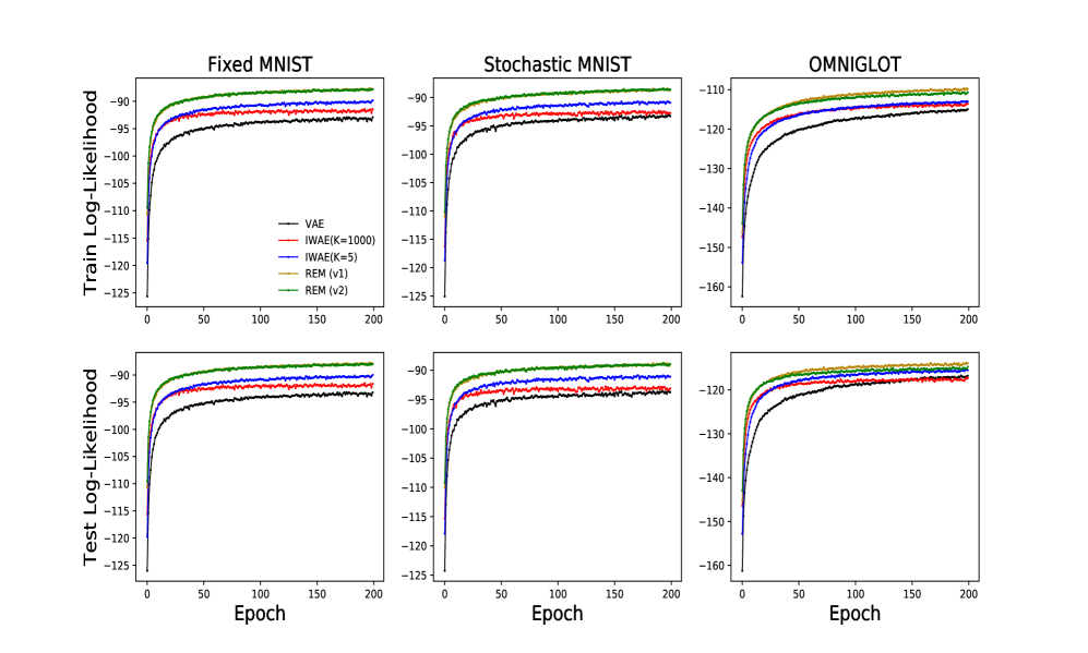
Figure 1: rem achieves significantly better performance than the vae and the iwae on three benchmark datasets in terms of log-likelihood (the higher the better).

5.1 Datasets

We evaluated all methods on the omniglot dataset and two versions of mnist. The omniglot is a dataset of handwritten characters in a total of $50$ different alphabets (Lake et al., 2013). Each of the characters is a single-channel image with dimension $28\times 28$. There are in total $24{,}345$ images in the training set and $8{,}070$ images in the test set. mnist is a dataset of images of handwritten digits introduced by LeCun et al. (1998). The first version of mnist we consider is the fixed binarization of the mnist dataset used by Larochelle and Murray (2011). The second version of mnist corresponds to random binarization; a random binary sample of digits is newly created during optimization to get a minibatch of data. In both cases the images are single-channel and have dimension $28\times 28$. There are $60{,}000$ images in the training set and $10{,}000$ images in the test set. All these datasets are available online at https://github.com/yburda/iwae.

5.2 Settings

We used the same network architecture for all methods. We followed Burda et al. (2015) and set the generative model, also called a decoder, to be a fully connected feed-forward neural network with two layers where each layer has $200$ hidden units. We set the recognition network, also called an encoder, to be a fully connected feed-forward neural network with two layers and $200$ hidden units in each layer. We use two additional linear maps to get the mean and the log-variance for the distribution $r_{\eta}(\bm{z}\,|\,\bm{x})$. The actual variance is obtained by exponentiating the log-variance.

We used a minibatch size of $20$ and set the learning rate following the schedule describes in Burda et al. (2015) with an initial learning rate of $10^{-3}$. We use this same learning rate schedule for both the learning of the generative model and the recognition network. We set the dimension of the latents used as input to the generative model to $20$. We set the seed to $2019$ for reproducibility. We set the number of particles $K$ to $1{,}000$ for both training and testing. We ran all methods for $200$ epochs. We used Amazon EC-2 P3 GPUs for all our experiments.

5.3 Results

We now describe the results in terms of quality of the learned generative model and proposal.

em-based methods learn better generative models.  We assess the quality of the fitted generative model for each method using log-likelihood. We report log-likelihood on both the training set and the test set. Figure 1 illustrates the results. The vae performs the worse on all datasets and on both the training and the test set. The iwae performs better than the vae as it optimizes a better objective function to train its generative model. Finally, both versions of rem significantly outperform the iwae on all cases. This is evidence of the effectiveness of em as a good alternative for learning deep generative models.

Recognition networks are good proposals.  Here we study the effect of the proposal on the performance of rem. We report the log-likelihood on both the train and the test set in Table 5.3. As shown in Table 5.3, using the richer distribution $s(\bm{z})$ does not always lead to improved performance. These results suggest that recognition networks are good proposals for updating model parameters in deep generative models.

Table 2: rem (v1) outperforms rem (v2) on all but one dataset. This suggests that recognition networks are effective proposals for the purpose of learning the generative model.

rem		Fixed MNIST		Stochastic MNIST		Omniglot
Proposal	Hyperproposal	Train	Test	Train	Test	Train	Test
$r_{\eta}(\bm{z}\,|\,\bm{x})$	$s(\bm{z})$	87.77	87.91	$88.68$	$88.95$	109.84	113.94
$s(\bm{z})$	$r_{\eta}(\bm{z}\,|\,\bm{x})$	$87.84$	$87.99$	88.58	88.92	$110.63$	$114.73$

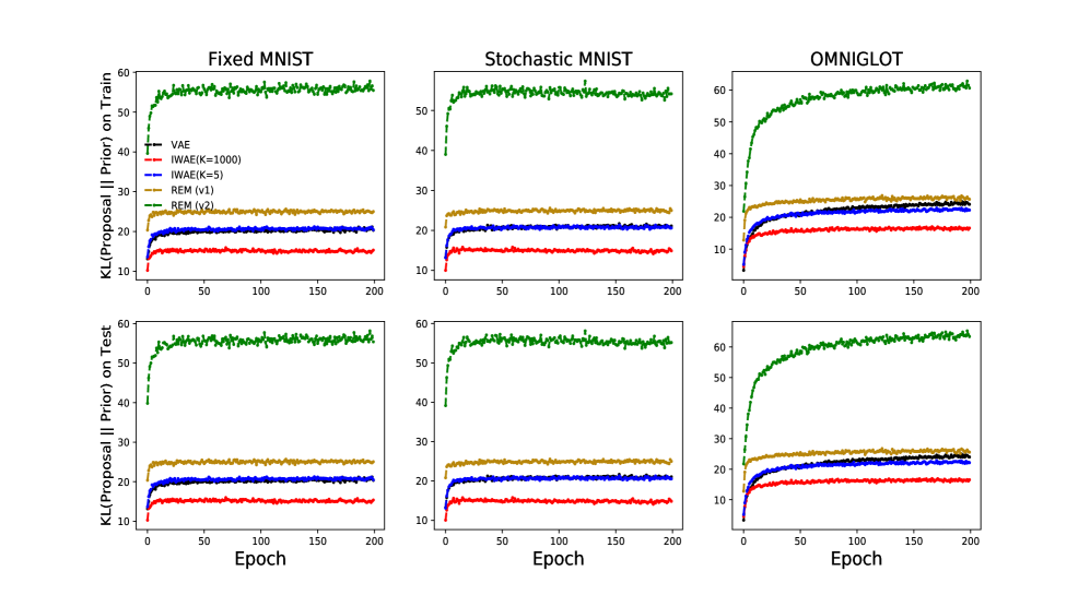
Figure 2: rem learns a better proposal than the vae and the iwae. This figure also shows that the quality of the iwae’s fitted posterior deteriorates as $K$ increases.

The inclusive KL is a better hyperobjective.  We also assessed the quality of the learned proposal for each method. We use the kl from the fitted proposal to the prior as a quality measure. This form of kl is often used to assess latent variable collapse. Figure 2 shows rem learns better proposals than both the iwae and the vae. It also confirms the quality of the iwae degrades when the number of particles $K$ increases.

6 Discussion

We considered expectation maximization (em) as an alternative to variational inference (vi) for fitting deep generative models. We rediscovered the importance weighted auto-encoder (iwae) as an instance of em and proposed a better algorithm for fitting deep generative models called reweighted expectation maximization (rem). rem decouples the learning dynamics of the generative model and the recognition network using a rich distribution found by moment matching. This avoids co-adaptation between the generative model and the recognition network. In several density estimation benchmarks, we found rem significantly outperforms the variational auto-encoder (vae) and the iwae in terms of log-likelihood. Our results suggest we should reconsider vi as the method of choice for fitting deep generative models. In this paper, we have shown em is a good alternative.

Future work includes applying the moment matching technique used in rem to improve variational sequential Monte Carlo techniques (Naesseth et al., 2017; Maddison et al., 2017; Le et al., 2017) or using rem together with doubly-reparameterized gradients (Tucker et al., 2018) to fit discrete latent variable models.

Acknowledgements.   We thank Scott Linderman, Jackson Loper, and Francisco Ruiz for their comments. ABD is supported by a Google PhD Fellowship.

References

- Alemi et al. (2017) Alemi, A. A., Poole, B., Fischer, I., Dillon, J. V., Saurous, R. A., and Murphy, K. (2017). Fixing a broken elbo. arXiv preprint arXiv:1711.00464.
- Bishop (2006) Bishop, C. M. (2006). Pattern recognition and machine learning. springer.
- Blei et al. (2017) Blei, D. M., Kucukelbir, A., and McAuliffe, J. D. (2017). Variational inference: A review for statisticians. Journal of the American Statistical Association, 112(518):859–877.
- Bornschein and Bengio (2014) Bornschein, J. and Bengio, Y. (2014). Reweighted wake-sleep. arXiv preprint arXiv:1406.2751.
- Bowman et al. (2015) Bowman, S. R., Vilnis, L., Vinyals, O., Dai, A. M., Jozefowicz, R., and Bengio, S. (2015). Generating sentences from a continuous space. arXiv preprint arXiv:1511.06349.
- Burda et al. (2015) Burda, Y., Grosse, R., and Salakhutdinov, R. (2015). Importance weighted autoencoders. arXiv preprint arXiv:1509.00519.
- Chen et al. (2016) Chen, X., Kingma, D. P., Salimans, T., Duan, Y., Dhariwal, P., Schulman, J., Sutskever, I., and Abbeel, P. (2016). Variational lossy autoencoder. arXiv preprint arXiv:1611.02731.
- Cremer et al. (2018) Cremer, C., Li, X., and Duvenaud, D. (2018). Inference suboptimality in variational autoencoders. arXiv preprint arXiv:1801.03558.
- Dayan and Hinton (1997) Dayan, P. and Hinton, G. E. (1997). Using expectation-maximization for reinforcement learning. Neural Computation, 9(2):271–278.
- Dayan et al. (1995) Dayan, P., Hinton, G. E., Neal, R. M., and Zemel, R. S. (1995). The Helmholtz machine. Neural Computation, 7(5):889–904.
- Dempster et al. (1977) Dempster, A. P., Laird, N. M., and Rubin, D. B. (1977). Maximum likelihood from incomplete data via the em algorithm. Journal of the Royal Statistical Society: Series B (Methodological), 39(1):1–22.
- Dieng et al. (2018) Dieng, A. B., Kim, Y., Rush, A. M., and Blei, D. M. (2018). Avoiding latent variable collapse with generative skip models. arXiv preprint arXiv:1807.04863.
- Dinh et al. (2016) Dinh, L., Sohl-Dickstein, J., and Bengio, S. (2016). Density estimation using real nvp. arXiv preprint arXiv:1605.08803.
- Goodfellow et al. (2014) Goodfellow, I., Pouget-Abadie, J., Mirza, M., Xu, B., Warde-Farley, D., Ozair, S., Courville, A., and Bengio, Y. (2014). Generative adversarial nets. In Advances in neural information processing systems, pages 2672–2680.
- Gregor et al. (2015) Gregor, K., Danihelka, I., Graves, A., Rezende, D. J., and Wierstra, D. (2015). Draw: A recurrent neural network for image generation. arXiv preprint arXiv:1502.04623.
- Gregor et al. (2013) Gregor, K., Danihelka, I., Mnih, A., Blundell, C., and Wierstra, D. (2013). Deep autoregressive networks. arXiv preprint arXiv:1310.8499.
- He et al. (2019) He, J., Spokoyny, D., Neubig, G., and Berg-Kirkpatrick, T. (2019). Lagging inference networks and posterior collapse in variational autoencoders. arXiv preprint arXiv:1901.05534.
- Higgins et al. (2017) Higgins, I., Matthey, L., Pal, A., Burgess, C., Glorot, X., Botvinick, M., Mohamed, S., and Lerchner, A. (2017). beta-vae: Learning basic visual concepts with a constrained variational framework. In International Conference on Learning Representations, volume 3.
- Hinton (2009) Hinton, G. E. (2009). Deep belief networks. Scholarpedia, 4(5):5947.
- Hinton et al. (1995) Hinton, G. E., Dayan, P., Frey, B. J., and Neal, R. M. (1995). The" wake-sleep" algorithm for unsupervised neural networks. Science, 268(5214):1158–1161.
- Hinton et al. (2006) Hinton, G. E., Osindero, S., and Teh, Y.-W. (2006). A fast learning algorithm for deep belief nets. Neural computation, 18(7):1527–1554.
- Hoffman and Johnson (2016) Hoffman, M. D. and Johnson, M. J. (2016). Elbo surgery: yet another way to carve up the variational evidence lower bound. In Workshop in Advances in Approximate Bayesian Inference, NIPS.
- Jordan et al. (1999) Jordan, M. I., Ghahramani, Z., Jaakkola, T. S., and Saul, L. K. (1999). An introduction to variational methods for graphical models. Machine learning, 37(2):183–233.
- Kingma et al. (2016) Kingma, D. P., Salimans, T., Jozefowicz, R., Chen, X., Sutskever, I., and Welling, M. (2016). Improved variational inference with inverse autoregressive flow. In Advances in neural information processing systems, pages 4743–4751.
- Kingma and Welling (2013) Kingma, D. P. and Welling, M. (2013). Auto-encoding variational bayes. arXiv preprint arXiv:1312.6114.
- Lake et al. (2013) Lake, B. M., Salakhutdinov, R. R., and Tenenbaum, J. (2013). One-shot learning by inverting a compositional causal process. In Advances in neural information processing systems, pages 2526–2534.
- Larochelle and Murray (2011) Larochelle, H. and Murray, I. (2011). The neural autoregressive distribution estimator. In Proceedings of the Fourteenth International Conference on Artificial Intelligence and Statistics, pages 29–37.
- Le et al. (2017) Le, T. A., Igl, M., Rainforth, T., Jin, T., and Wood, F. (2017). Auto-encoding sequential monte carlo. arXiv preprint arXiv:1705.10306.
- Le et al. (2018) Le, T. A., Kosiorek, A. R., Siddharth, N., Teh, Y. W., and Wood, F. (2018). Revisiting reweighted wake-sleep. arXiv preprint arXiv:1805.10469.
- LeCun et al. (1998) LeCun, Y., Bottou, L., Bengio, Y., Haffner, P., et al. (1998). Gradient-based learning applied to document recognition. Proceedings of the IEEE, 86(11):2278–2324.
- Liang et al. (2018) Liang, D., Krishnan, R. G., Hoffman, M. D., and Jebara, T. (2018). Variational autoencoders for collaborative filtering. In Proceedings of the 2018 World Wide Web Conference on World Wide Web, pages 689–698. International World Wide Web Conferences Steering Committee.
- Maddison et al. (2017) Maddison, C. J., Lawson, J., Tucker, G., Heess, N., Norouzi, M., Mnih, A., Doucet, A., and Teh, Y. (2017). Filtering variational objectives. In Advances in Neural Information Processing Systems, pages 6573–6583.
- Minka et al. (2005) Minka, T. et al. (2005). Divergence measures and message passing. Technical report, Technical report, Microsoft Research.
- Murphy (2012) Murphy, K. P. (2012). Machine learning: a probabilistic perspective. MIT press.
- Naesseth et al. (2017) Naesseth, C. A., Linderman, S. W., Ranganath, R., and Blei, D. M. (2017). Variational sequential monte carlo. arXiv preprint arXiv:1705.11140.
- Neal (1992) Neal, R. M. (1992). Connectionist learning of belief networks. Artificial intelligence, 56(1):71–113.
- Owen (2013) Owen, A. B. (2013). Monte Carlo theory, methods and examples. Book in preparation.
- Rainforth et al. (2018) Rainforth, T., Kosiorek, A. R., Le, T. A., Maddison, C. J., Igl, M., Wood, F., and Teh, Y. W. (2018). Tighter variational bounds are not necessarily better. arXiv preprint arXiv:1802.04537.
- Razavi et al. (2019) Razavi, A., Oord, A. v. d., Poole, B., and Vinyals, O. (2019). Preventing posterior collapse with delta-vaes. arXiv preprint arXiv:1901.03416.
- Rezende and Mohamed (2015) Rezende, D. J. and Mohamed, S. (2015). Variational inference with normalizing flows. arXiv preprint arXiv:1505.05770.
- Rezende et al. (2014) Rezende, D. J., Mohamed, S., and Wierstra, D. (2014). Stochastic backpropagation and approximate inference in deep generative models. arXiv preprint arXiv:1401.4082.
- Salakhutdinov and Hinton (2009) Salakhutdinov, R. and Hinton, G. (2009). Deep boltzmann machines. In Artificial intelligence and statistics, pages 448–455.
- Sønderby et al. (2016) Sønderby, C. K., Raiko, T., Maaløe, L., Sønderby, S. K., and Winther, O. (2016). How to train deep variational autoencoders and probabilistic ladder networks. In 33rd International Conference on Machine Learning (ICML 2016).
- Song et al. (2016) Song, Z., Henao, R., Carlson, D., and Carin, L. (2016). Learning sigmoid belief networks via monte carlo expectation maximization. In Artificial Intelligence and Statistics, pages 1347–1355.
- Tucker et al. (2018) Tucker, G., Lawson, D., Gu, S., and Maddison, C. J. (2018). Doubly reparameterized gradient estimators for monte carlo objectives. arXiv preprint arXiv:1810.04152.
- Zhao et al. (2018) Zhao, T., Lee, K., and Eskenazi, M. (2018). Unsupervised discrete sentence representation learning for interpretable neural dialog generation. arXiv preprint arXiv:1804.08069.