Global Energetics of Solar Flares: VII. Aerodynamic Drag in Coronal Mass Ejections

Abstract

The free energy that is dissipated in a magnetic reconnection process of a solar flare, generally accompanied by a coronal mass ejection (CME), has been considered as the ultimate energy source of the global energy budget of solar flares in previous statistical studies. Here we explore the effects of the aerodynamic drag force on CMEs, which supplies additional energy from the slow solar wind to a CME event, besides the magnetic energy supply. For this purpose we fit the analytical aerodynamic drag model of Cargill (2004) and Vrsnak et al. (2013) to the height-time profiles $r(t)$ of LASCO/SOHO data in 14,316 CME events observed during the first 8 years (2010-2017) of the SDO era (ensuring EUV coverage with AIA). Our main findings are: (i) a mean solar wind speed of $w=472\pm 414$ km s^-1, (ii) a maximum drag-accelerated CME energy of $E_{drag}\lower 1.72218pt\hbox{$\;\buildrel<\over{\scriptstyle\sim}\;$}2\times 10^{32}$ erg, (iii) a maximum flare-accelerated CME energy of $E_{flare}\lower 1.72218pt\hbox{$\;\buildrel<\over{\scriptstyle\sim}\;$}1.5\times 10^{33}$ erg; (iv) the ratio of the summed kinetic energies of all flare-accelerated CMEs to the drag-accelerated CMEs amounts to a factor of 4; (v) the inclusion of the drag force slightly lowers the overall energy budget of CME kinetic energies in flares from $\approx 7\%$ to $\approx 4\%$; and (vi) the arrival times of CMEs at Earth can be predicted with an accuracy of $\approx 23\%$.

1 INTRODUCTION

The motivation for this study is the determination of the energy budget of coronal mass ejections (CMEs) in the overall global energetics and energy partitioning of solar flare/CME events. Previous statistical work on flare energies has been pioneered by Emslie et al. (2004, 2005, 2012), and has been focused to the dissipation of magnetic energies (Aschwanden et al. 2014), thermal energies (Aschwanden et al. 2015), non-thermal energies (Aschwanden et al. 2016), CMEs (Aschwanden 2016, 2017), and the global energy closure between these various forms of energies (Aschwanden et al. 2017). It goes without saying that we cannot claim to understand the physics of flares and CMEs if we cannot pin down the relative amounts of energies in such a way that we obtain closure in the total energy budget. In the big picture we assumed that the magnetic free energy (which is defined as the difference between the non-potential and potential magnetic energy) provides the ultimate source and upper limit of energy that can be dissipated during a flare/CME event, most likely to be driven by a magnetic reconnection process. Consequently, the potential gravitational force and the kinetic energy of a CME have to be supplied entirely by the magnetic free energy and the associated Lorentz forces, in addition to the energy needed for the acceleration of particles and direct heating of the flare plasma. In the meantime it became clear that additional energy (besides the dissipated magnetic energy) can supply part of the CMEs kinematics, in form of the aerodynamic drag force that is exerted onto CMEs from the ambient slow solar wind (Vrsnak and Gopalswamy 2002; Cargill 2004; Vrsnak et al. 2008, 2010, 2013). For a brief review see Aschwanden (2019, Section 15.5). The main focus of this study is therefore the question to what extent the presence of the aerodynamic drag force affects the energy partition ratios of flare/CME events, compared with previous studies where this effect was not taken into account.

The role of the aerodynamic drag force on coronal mass ejections (CMEs) and interplanetary coronal mass ejections (ICME) has been brought to recent attention (Cargill 2004; Chen 1997; Gopalswamy et al. 2001a). Cargill (2004) demonstrated that tenuous ICMEs rapidly equalize in velocity due to the very effective drag force, while ICMEs that are denser than the ambient solar wind are less affected by the aerodynamic drag, although the drag coefficient is approximately independent of the propagation distance. An anti-correlation between the CME acceleration and velocity was established from LASCO/SOHO data (Gopalswamy et al. 2000, 2001a), which confirms that massive CMEs are less affected by the aerodynamic drag (Vrsnak et al. 2008). Massive CMEs have been found to be accelerated for masses of $m_{cme}>3\times 10^{14}$ g, while less massive CMEs are generally decelerated (Michalek 2012). The shortest transit times and hence the fastest velocities have been identified in narrow and massive ICMEs (i.e., high-density eruptions) propagating in high-speed solar wind streams (Gopalswamy et al. 2000, 2001a; Vrsnak et al. 2010). Extremely short transit times of 14 hours (Gopalswamy et al. 2005a) and 21 hours have been observed (Temmer and Nitta 2005), with maximum speeds of $v\approx 2600$ km s^-1, but agreement with the aerodynamic drag model requires a decrease of the solar wind density near 1 AU (Temmer and Nitta 2015), but see Gopalswamy et al. (2016) for an alternative interpretation. Fast CMEs were found to show a linear dependence for the velocity difference between CMEs and solar wind, while slow CMEs show a quadratic dependence (Maloney and Gallagher 2010). A quadratic dependence is expected in a collisionless environment, where drag is caused primarily by emission of magnetohydrodynamic (MHD) waves (Vrsnak et al. 2013). A distinction between the aerodynamic drag force and the hydrodynamic Stokes drag force has been suggested (Iju et al. 2014), but was found to be equivalent in other cases (Gopalswamy et al. 2001b). Analytical models for the drag coefficient include the viscosity in the turbulent solar wind (Subramanian et al. 2012). The aerodynamic drag model has been used increasingly as the preferred physical model to quantify the propagation of ICMEs and to forecast their arrival times at Earth, and this way it became a key player in space weather predictions (Michalek et al. 2004; Vrsnak et al. 2010; Song 2010; Shen et al. 2012; Kilpua et al. 2012; Lugaz and Kintner 2013; Hess and Zhang 2014 ; Tucker-Hood et al. 2014; Mittal and Narain 2015; Zic et al. 2015; Sachdeva et al. 2015; Dumbovic et al. 2018; Verbeke et al. 2019). Arrival times at Earth inferred from the “drag-based model” have been compared with the numerical “WSA-ENLIL+Cone model” (Wang-Sheeley-Arge), which enables early space-weather forecast 2-4 days before the arrival of the disturbance at Earth (Vrsnak et al. 2014; Dumbovic et al. 2018). The Stokes form was the basis for the empirical shock arrival model, whose prediction is comparable to that of the ENLIL+cone model (Gopalswamy et al. 2005b, 2013). New models, such as the Forecasting a CMEs Altered Trajectory (ForeCAT) deal also with CME reflections based on magnetic forces and non-radial drag coefficients (Kay et al. 2015). Geometric models, such as the Graduated Cylindrical Shell (GCS) model are fitted to LASCO and STEREO data, finding that the Lorentz forces generally peak at $(1.65-2.45)R_{\odot}$, and become negligible compared with the aerodynamic drag already at distances of $(3.5-4.0)R_{\odot}$, but only at $(12-50)R_{\odot}$ for slow CME events (Sachdeva et al. 2017).

In this paper we are fitting the aerodynamic drag model to all CMEs observed with LASCO/SOHO during the SDO era (2010-1017), which yields the physical parameters that are necessary to determine the kinetic energies, the energy ratios of flare-associated and drag-accelerated CMEs, as well as their arrival times near Earth. We present the analytical description of the constant-acceleration and aerodynamic drag model in Section 2, the data analysis of forward-fitting the analytical models to LASCO data and the related results in Section 3, a discussion of some relevant issues in Section 4 and conclusions in Section 5.

2 THEORY AND METHODS

2.1 The Constant-Acceleration Model

The simplest model of the kinematics of a coronal mass ejection (CME) has a minimum number of three free parameters, which includes a constant (time-averaged) acceleration $a_{0}$, an initial height $r(t=t_{0})=r_{0}$, and a starting time at a reference time $t=t_{0}$. A slightly more general model (with 4 free parameters) allows also for a non-zero velocity $v_{0}=v(t=t_{0})$ at the starting time $t=t_{0}$, which constitutes four free model parameters $[a_{0},v_{0},r_{0},t_{0}]$, defining the time dependence of the acceleration $a(t)$,

$$a(t)=a_{0}\ ,$$ (1)

the velocity $v(t)$ of the CME leading edge,

$$v(t)=\int_{t_{0}}^{t}a(t)dt=v_{0}+a_{0}(t-t_{0})\ ,$$ (2)

and the radial distance $r(t)$ from Sun center,

$$r(t)=\int_{t_{0}}^{t}v(t)\ dt=r_{0}+v_{0}(t-t_{0})+{a_{0}\over 2}(t-t_{0})^{2}\ .$$ (3)

The radial distance $r(t)$, which is directly obtained from the observations, can be fitted with a simple second-order polynomial,

$$r(t)=c_{0}+c_{1}t+c_{2}t^{2}\ ,$$ (4)

where the free parameters as functions of the coefficients $c_{0},c_{1},c_{2}$ follow directly from Eqs. (3) and (4),

$$a_{0}=2c_{2}\ ,$$ (5)

$$t_{0}=(v_{0}-c_{1})/a_{0}\ ,$$ (6)

$$r_{0}=c_{0}+v_{0}t_{0}-{a_{0}\over 2}t_{0}^{2}\ .$$ (7)

A practical example of the height-time profile $r(t)$, the velocity profile $v(t)$, and the acceleration profile $a(t)$ of the constant-acceleration CME kinematic model is shown for an event in Fig. 1 (left), where the observed datapoints $r_{i}=r(t=t_{i})$ are marked with crosses (top left panel), and the fitted model is rendered with thick curves, covering the fitted time range $[t_{1},t_{2}]$. For the fitting of an acceleration model to LASCO data we have to be aware that CMEs are observed at a heliocentric distance of $\lower 1.72218pt\hbox{$\;\buildrel>\over{\scriptstyle\sim}\;$}2.5R_{\odot}$, by which time most CMEs have finished acceleration (Bein et al. 2011) and we are observing a residual acceleration only, combined with gravity and drag.

For the calculation of the CME starting time $t_{s}$ we extrapolate the model $r(t)$, which is observed in the time range $[t_{1},t_{2}]$, to an expanded range $[t_{0},t_{2}]$ with double length (with lower boundary $t_{0}=t_{1}-(t_{2}-t_{1})$). The actual starting time $t_{s}$ of the CME launch can now be derived from the height-time profile $r(t)$ within the expanded time range $[t_{0},t_{2}]$, where two possible cases can occur. One case is when the extrapolated minimum height at the start of the CME is lower than the solar limb, in which case the solution $r(t)$ can simple be extrapolated to the nominal height $r_{s}=1R_{\odot}$, as it is shown for the case depicted in Fig. 1 (left), for the CME event on 2011 September 24, 18:36 UT.

The other case is when the minimum height $r_{s}=min[r(t)]=r(t=t_{s})$ is higher than the solar limb $(r_{min}>R_{\odot})$, in which case the starting time $t_{s}$ coincides with the height minimum, where the velocity is zero, i.e., $v_{s}=v(t=t_{s})=0$. An example of the second case is shown in Fig. 2 (left), where the starting height is estimated to $r_{s}=1.963R_{\odot}$ for the event of 2010 January 3, 05:30 UT. Note that the starting time, defined by the extrapolated zero velocity $v_{s}(t=t_{s})=0$, is dependent on the model, estimated at $t_{s}=2.375$ hrs for the constant-acceleration model, and $t_{s}=6.287$ hrs for the aerodynamic drag model. So there is an uncertainty of the order of $\approx 4$ hrs for the start of this particular event.

2.2 The Aerodynamic Drag Model

We define now, besides the constant-acceleration model, a second model that is based on a physical mechanism. The interaction of a coronal mass ejection (CME) (or an interplanetary coronal mass ejection (ICME)) with the solar wind leads to an adjustment or equalization of their velocities at heliocentric distances from a few solar radii out out to one astronomical unit. When an ICME has initially a higher velocity (or take-off speed) than the solar wind, it is then slowed down to a lower value that is closer to the solar wind speed (Fig. 1). Vice versa, ICMEs with slower speeds than the ambient solar wind speed become accelerated to about the solar wind speed (Fig. 2). There are also cases where the CME accelerates to high speeds, but quickly slows down even before the solar wind formation (Gopalswamy et al. 2012; 2017). Following the physical model of aerodynamic drag formulated by Cargill (2004) and the analytical solution of Vrsnak et al. (2013), we can describe the velocity time profile $v(t)$,

$$v(t)=\left({dr(t)\over dt}\right)={(v_{s}-w)\over 1\pm\gamma(v_{s}-w)(t-t_{s})}+w\ ,$$ (8)

where $v_{s}$ is the CME velocity at an initial start time $t_{s}$ (also called “take-off” velocity), $w$ is the (constant) solar wind speed, $\gamma\approx 1\times 10^{-7}$ cm^-1 is the drag parameter (in units of inverse length), and $r_{s}$ is the initial height at the starting time $t=t_{s}$. The drag parameter $\gamma$ has been defined as

$$\gamma={c_{d}A\rho_{w}\over M+M_{v}}\ ,$$ (9)

where $c_{d}$ is the dimensionless drag coefficient (Cargill 2004), $A$ is the ICME cross-sectional area, $\rho_{s}$ is the ambient solar-wind density, and $M$ is the ICME mass. The so called virtual mass, $M_{v}$, can be expressed approximately as $M_{v}\approx\rho_{w}V/2$, where $V$ is the ICME volume. Here we assumed a constant solar wind speed $w$ and a constant $\gamma$, which is justified to some extent by MHD simulations (Cargill 2004), which show the constant drag coefficient $c_{d}$ varies slowly between the Sun and 1 AU, and is of order unity. When the ICME and solar wind densities are similar, $c_{d}$ becomes larger, but remains approximately constant with radial distance. For ICMEs denser than the ambient solar wind, $\gamma$ is approximately independent of radius, while $\gamma$ falls off linearly with distance for tenuous ICMEs (Cargill 2004). Regarding the variability of the solar wind speed $w(r)$ as a function of the distance $r$, the largest deviation from a constant value $w(r)$ is expected in the corona, where the solar wind transitions from subsonic to supersonic speed at a distance of a few solar radii from Sun center, but this coronal zone is also the place where flare-associated acceleration of CMEs occurs and aerodynamic drag is less dominant, which alleviates the influence of the (non-constant) solar wind.

Vrsnak et al. (2003) integrated the velocity dependence $v(t)$ (Eq. 8) to obtain an analytical function for the height-time profile $r(t)$ explicitly,

$$r(t)=\pm{1\over\gamma}\ln{[1\pm\gamma(v_{s}-w)(t-t_{s})]}+w(t-t_{s})+r_{s}\ .$$ (10)

Differentiating the speed $v(t)$, we obtain an analytical expression for the acceleration time profile $a(t)$,

$$a(t)=\left({dv(t)\over dt}\right)={\mp\gamma(v_{s}-w)^{2}\over[1\pm\gamma(v_{s}-w)(t-t_{s})]^{2}}\ .$$ (11)

We see that this model has 5 free parameters $[t_{s},v_{s},r_{s},w,\gamma]$. The two regimes of $\pm$ correspond to the deceleration/acceleration regime, i.e., it is plus for $v_{s}>w$, and minus for $v_{s}<w$. Comparing with the constant-acceleration model, we see that three parameters are equivalent, i.e., $[t_{s},r_{s},v_{s}]=[t_{0},r_{0},v_{0}]$, while the acceleration $a_{0}$ is constrained by the drag coefficient $\gamma$ and the solar wind speed $w$.

Two examples of CME kinematic models with the aerodynamic drag model are shown in Figs. 1 and 2 (right-hand panels). The case shown in Fig. 1 (middle right panel) reveals deceleration from and initial value of $v_{s}=801$ km s^-1 towards the solar wind speed of $w=405$ km s^-1, while the other case shows acceleration from $v_{s}=0$ km s^-1 to $w=421$ km s^-1, according to the aerodynamic drag model (Fig.2, middle right panel).

For the calculation of the free parameters we define a fitting time range $[t_{s},t_{2}]$ that is bound by the starting time $t_{s}$ of the CME (inferred from the constant-acceleration model) and the last observed time $t_{2}$ of the LASCO/SOHO data. The remaining four free parameters $[r_{s},v_{s},w,\gamma]$ are optimized by forward-fitting of the height-time profile $r(t)$ (Eq. 10) to the observed heights $r_{i}=r(t_{i}),i=0,...,n_{t}$ of the LASCO/SOHO data, using the Direction Set (Powell’s) methods in multidimensions (Press et al. 1986). A robust performance of this optimization algorithm is achieved by optimizing the parameters [$ln(w)$, $\ln(v_{s}/w)$, $\ln{(\gamma)}$, $r_{s}/R_{\odot}$]. The iteration of logarithmic parameters avoids (unphysical) negative values for the velocities and the drag parameter, [$v_{s},w,\gamma$].

3 OBSERVATIONS AND DATA ANALYSIS RESULTS

3.1 LASCO/SOHO Data

In the following we describe the observations from LASCO/SOHO and characterize the statistical results of our data analysis. We make use of the SOHO/LASCO CME catalog that is publicly available at https://cdaw.gsfc.nasa.gov/CME$\_$list, based on visually selected CME events, created and maintained by Seiji Yashiro and Nat Gopalswamy (Yashiro et al. 2008; Gopalswamy et al. 2009a, 2010). A brief description of the algorithm of measuring height-time profiles $r(t)$ is given on the same website. From the LASCO/SOHO data archive, only C2 and C3 data have been used for uniformity, because LASCO/C1 has been disabled in June 1998. We downloaded the time sequences of height time profiles, $r_{i}=r(t=t_{i}),i=1,...,n_{t}$, that are available for every CME detected with LASCO/SOHO during the first 8 years (2010-2017) of the Solar Dynamics Observatory (SDO) mission. This data set comprises 14,316 events, covering almost a full solar cycle.

3.2 Fitting of CME Kinematic Models

The forward-fitting of both the constant-acceleration model (Section 2.1) and the aerodynamic drag model (Section 2.2) to the LASCO height-time profiles yields dynamical parameters that are important for extrapolating the CME kinematics from the LASCO-covered distance range of $r\approx(3-32)R_{\odot}$ to the lower corona at $r\lower 1.72218pt\hbox{$\;\buildrel<\over{\scriptstyle\sim}\;$}1.5R_{\odot}$ (for identification of simultaneous flare events), and extrapolating out into the heliosphere to $r\approx 1$ AU (for forecasting of the CME arrival time at Earth).

We fitted the constant-acceleration model (Section 2.1) to the LASCO/SOHO CME height-time profiles in the same way as the second-order polynomial fits have been carried out in the LASCO CME catalog, and we verified consistency between our fits and those listed in the CDAW LASCO CME catalog. We found that the forward-fitting of both models is fairly robust. Unsatisfactory fits have been found in very few cases, identified by a low fitting accuracy ($\sigma\lower 1.72218pt\hbox{$\;\buildrel<\over{\scriptstyle\sim}\;$}5\%$, in 6% of the cases for the constant-acceleration model, and in 7% of the cases for the aerodynamic drag model), or a low drag coefficient ($\gamma\leq 10^{-8}$ cm^-1, in 10% of the cases).

The fitting quality of the two (analytical) theoretical models used here is defined as follows. We calculate the average ratios of the fitted (modeled) distances $r_{i}^{model}$ and compare them with the observed distances, $r_{i}^{obs}=r(t_{i}),i=1,...,n_{t}$,

$$q={1\over n_{t}}\sum_{i=1}^{n_{t}}\left({r_{i}^{model}\over r_{i}^{obs}}\right)\approx 1.0\pm\sigma\ .$$ (12)

This measure of the accuracy has been found to be very suitable, yielding a standard deviation of $\sigma_{CA}=2.7\%\pm 2.7\%$ for the constant-acceleration model, and a very similar value of $\sigma_{AD}=2.9\%\pm 2.5\%$ for the aerodynamic drag model. The accuracies were calculated for all 14,316 events, based on an average of $n_{t}\approx 23$ distance measurements per event. The fact that both models fit the data with equal accuracy suggests that either model is suitable. The example shown in Fig. 1 reveals an equal accuracy of $\sigma_{AC}=\sigma_{AD}=4.4\%$ for both models. The example shown in Fig. 2 yields a better performance for the constant-acceleration model ($\sigma_{CA}=3.3\%$), versus $\sigma_{AD}=5.4\%$ for the aerodynamic drag model. However, the aerodynamic drag model represents a physical model and yields the five parameters $[t_{s},r_{s},v_{s},w,\gamma]$, while the constant-acceleration model requires four parameters $[t_{0},r_{0},v_{0},a_{0}]$. A fundamental difference between the two models is that the acceleration $a_{0}$ is not time-dependent in the constant-acceleration model, while it is variable in the aerodynamic drag model, and the CME speed asymptotically approaches the solar wind speed constraining the solar wind speed $w$ and the aerodynamic drag coefficient $\gamma$.

3.3 Eruptive and Failed CMEs

A distinction is generally made by the dynamical characteristics of CME events, which defines the type of eruptive flares or CMEs when the final CME speed exceeds the gravitational escape velocity ($v_{2}\geq v_{esc}$), and alternatively the type failed eruptions, when the escape velocity is not reached ($v_{s}<v_{esc}$). Failed eruptions have mass motions, but do not escape (Gopalswamy et al. 2009b). The escape speed depends only on the radial distance from the Sun center,

$$v_{esc}(r)=\sqrt{{2GM_{\odot}\over r}}\approx 618\ \left({r\over R_{\odot}}\right)^{-1/2}{\rm km\ s}^{-1}\ ,$$ (13)

where $G$ is the gravitational constant, $M_{\odot}$ the solar mass, and $R_{\odot}$ the solar radius. Examples of the escape speed dependence on the radial distance are shown in Figs. 1 and 2 (middle panels), where the escape speed is indicated with dotted curves. In the first event, the CME speed exceeds the escape velocity all the times (Fig. 1 middle right), while the second case reaches escape speed at $t=12.1$ hrs (Fig. 2, middle right), which is reached at a distance of $r=7.2R_{\odot}$ (Fig. 2 top right). So, both events are eruptive CMEs.

We determined the time $t_{esc}$ and distance $r_{esc}$ where the CME gained sufficient speed to overcome the combined Lorentz force, gravitational force, and drag force, as a function of the time (Fig. 3a) and as a function of the distance (Fig. 3b), for all analyzed 14,316 CME events. The start time $t_{s}$ has been extrapolated from the aerodynamic drag model to a starting height of $r_{s}\approx 1R_{\odot}$. We see that $\approx 10\%$ of the CMEs reach escape velocity below the solar limb (Fig. 3b), that $\approx 30\%$ of the CMEs reach escape velocity at $r_{1}\lower 1.72218pt\hbox{$\;\buildrel<\over{\scriptstyle\sim}\;$}3R_{\odot}$, at the location of the LASCO first detection, and that 100% reach escape speed at a distance of $r_{2}\lower 1.72218pt\hbox{$\;\buildrel<\over{\scriptstyle\sim}\;$}10R_{\odot}$, at the location of the LASCO last detection. Conversely, all CMEs reach escape velocity at $\lower 1.72218pt\hbox{$\;\buildrel<\over{\scriptstyle\sim}\;$}25$ hrs after launch (Fig. 3a). This confirms the selection criterion of the CDAW CME list, where eruptive CME events have been measured only, by definition. No confined flare is contained in the CDAW CME list, but we will encounter such events when we compare the association of soft X-ray flare events with CME detections, using GOES flare data (see Section 3.5).

3.4 Statistical Results of LASCO Fitting

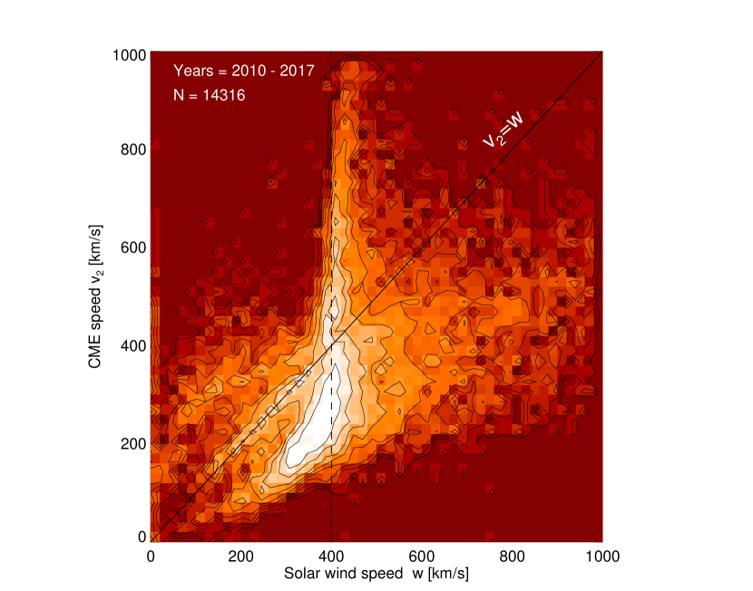
Figure 4: Comparison of final CME speed $v_{2}$ (at the last detection with LASCO) with the solar wind speed $w$, for all CME events. Equivalence of CME speed $v_{2}$ and wind speed $w$ is indicated with a diagonal line, while the vertical dashed line indicates a slow solar wind speed of $w=400$ km.

We summarize the statistical results of our fitting of the two CME kinematic models (Eqs. 3 and 10) in Table 1 and in the Figures 4 to 7. In Fig. 4 we show the near-final speed $v_{2}$ (that is measured from the last detection in LASCO data), versus the ambient slow solar wind speed $w$ for all CME events. Although the last detection with LASCO yields a wide range of final speeds $v_{2}\approx 100-1000$ km s^-1 (Fig. 4), the slow slow solar wind is mostly concentrated in the velocity range of $w\approx 200-500$ km s^-1. This implies that the aerodynamic drag model accelerates CMEs with $v_{s}<w$ and decelerates CMEs with $v_{s}>w$ towards the near-final speed of $v_{2}\approx 200-500$ km s^-1, as indicated with the concentration of data along the vertical ridge of $w\approx 400$ km s^-1 (Fig. 4). This agrees also with the conclusion obtained from the empirical acceleration formula derived by Gopalswamy et al. (2001b), i.e., $a=-0.0054(v_{cme}-406)$.

This confirms that the solar wind speed $w$ is reliably retrieved from forward-fitting of the kinematic model (Eq. 8) to the LASCO data, regardless what the value of the CME speed $v_{2}$ is. The most frequent starting height is in the lower corona, at a median distance of $r_{s}\lower 1.72218pt\hbox{$\;\buildrel<\over{\scriptstyle\sim}\;$}1.2R_{\odot}$ from Sun center ($h_{S}\lower 1.72218pt\hbox{$\;\buildrel<\over{\scriptstyle\sim}\;$}140,000$ km) (Fig. 5a, Table 1). The first detection with LASCO occurs at a mean distance of $r_{1}=(3.0\pm 0.8)R_{\odot}$ (Fig. 5b), while the last detection with LASCO is around $r_{2}=(10.3\pm 6.4)R_{\odot}$ (Fig. 5c, Table 1).

Statistics of the velocities are particularly interesting here because the propagation of most CMEs depends on their relative speed to the slow solar wind speed. The distribution of starting speeds $v_{s}$ has two peaks (Fig. 6a), one near $v_{s}\approx 0$, and a second peak at $v_{s}\approx 200$ km s^-1. This bimodality depends on the time resolution, which is typically 0.2 hrs or 12 minutes (Table 1) for LASCO data. If the initial acceleration of CMEs in the lower solar corona peaks before 12 minutes, we do not resolve the initial speed increase from $v_{s}=0$ to $v_{1}\approx 200$ km s^-1, while a peak acceleration later than 12 minutes after the starting time $t=t_{s}$ will reveal an initial value of $v_{s}\approx 0$ (e.g., Fig. 2). This explains the large range of obtained starting velocities $v_{s}=482\pm 1294$ km s^-1, which has a higher mean than that at the first detection with LASCO, $v_{1}=320\pm 283$ km s^-1 (Fig. 6b), or at the last detection with LASCO, $v_{2}=368\pm 198$ km s^-1 (Fig. 6c), due to the aerodynamic drag that streamlines the CME velocities.

The most interesting statistical result is the distribution of slow solar wind speeds, which have an average of $w=472\pm 414$ km s^-1 or a median of $w=405$ km s^-1 (Fig. 6d), obtained at heliocentric distances in the range of $r_{2}\approx 3-30R_{\odot}$, according to the last LASCO detection (shown in Fig. 5c). Note that these forward-fitting results of the aerodynamic drag model, based on 14,306 LASCO CME events, represent one of the largest statistical measurements of the slow solar wind speeds.

We present the statistical time scales related to the LASCO detection delay $(t_{1}-t_{s})$ and propagation duration in the LASCO field-of-view in Fig. 7 and Table 1. The average detection delay is $(t_{1}-t_{s})=1.0\pm 1.3$ hrs (Fig. 7a). The mean duration of CME propagation in the LASCO observed zone is $(t_{2}-t_{1})=4.3\pm 3.7$ hrs (Fig. 7b).

3.5 CME Start Times and GOES Flare Times

While the previously described results make exclusively use of LASCO/SOHO data, we compare now these measurements with other data sets based on HMI/SDO, AIA/SDO, and GOES data. In particular we focus on a subset of 576 M and X-class GOES flare events that have been observed during the first 7 years of the SDO mission (2010-2016), for which measurements of temporal, spatial, and energetic parameters were published previously (Aschwanden 2016, 2017).

In order to identify LASCO CME events that are associated with each of the 576 M and X-class GOES flares we use the GOES flare start reference times $t_{s}^{GOES}$ issued by NOAA, and find the CME events (of the entire LASCO catalog of 14,316 events during 2010-2017) that have their first LASCO detection time $t_{1}^{LASCO}$ closest to the starting time $t_{s}^{GOES}$ of the GOES flares. The relative time difference can be significantly improved by extrapolating the LASCO height-time plot $r(t)$ to the LASCO starting time $t_{s}^{LASCO}$ at the initial height of $r_{s}=r(t=t_{s})$, which yields a time difference between the GOES and LASCO starting times,

$$\Delta t=t_{s}^{LASCO}-t_{s}^{GOES}\ .$$ (14)

A histogram of the time differences between the GOES start times $t_{s}^{GOES}$ and the extrapolated LASCO starting times $t_{s}^{LASCO}$ is shown in Fig. 8. Out of the 576 events we find a total of 480 events (83%) with relative time delays within a time window of $\pm 4$ hrs. We calculate a Gaussian fit to the core distribution within a time window of $\pm 0.7$ hrs, which encompasses 231 events (40%) that may be considered as a lower limit of events with good time coincidence. The association rate of a CME with a flare increases from 20% for C-flares to 100% in large X-class events (Yashiro et al. 2005). Therefore, the flare-associated fraction of LASCO CME events may vary between the limits of 20% and 100%. On the other hand, the complementary fraction of GOES flare events that have no CME detected with LASCO may vary in the range of 17% to 60%. These CME-less events that are not associated with a $>$M.1 GOES class flare may consist of confined flares or weak non-detected CME events.

The distribution of starting delays is $\tau=t_{s}^{LASCO}-t_{s}^{GOES}=0.07\pm 0.28$ hrs (Fig. 8), evaluated with a Gaussian fit at the peak of the distribution. This is consistent with previous measurements of 275 flare/CME events, where also no significant delay was found, i.e., $\tau=0.02\pm 0.77$ hrs (Fig. 17c in Aschwanden 2016). In this relative timing analysis we neglected the difference of the heliographic position of CME source locations, since the propagation time difference from disk center to the limb, i.e., $\Delta t_{prop}=R_{\odot}/v_{cme}\approx 0.2$ hrs (for $v_{cme}\approx 1000$ km s^-1) is smaller than the bin width of the histogram shown in Fig. 8.

Four examples of flare/CME events are shown in form of GOES flux time profiles and CME height-time plots (Fig. 9), which illustrate different uncertainties in the time coincidence. The first example (Fig. 9a) exhibits a simple single-peak GOES time profile, where the GOES and LASCO starting times coincide within 0.174 hrs (or 10 minutes). The second example (Fig. 9b) has an extremely impulsive peak, but the extrapolated LASCO starting time has due to the low initial speed ($v_{1}=71$ km s^-1 at the first detection with LASCO) a large uncertainty, so that the coincidence is within 0.542 hrs or 33 minutes). The third case (Fig. 9c) exhibits a substantial uncertainty in the GOES starting time, so that the coincidence is within 0.40 hrs (or 24 minutes). The fourth example (Fig. 9d) shows an X-class flare with a well-defined starting time, but the initial CME speed is so low that it implies a large negative delay of -1.56 hrs (or 94 minutes). In summary, the accuracy of the relative time coincidence between soft X-ray emission (detected with GOES) and the starting height of CMEs (detected with LASCO) depends on the definition of the flaring time (starting, peak, or end time) and the uncertainties of the CME speed extrapolation, particularly in the case of slow CMEs.

Another time marker of CME starting times is the EUV dimming, which has been measured with large statistics using AIA data. A significant delay has been observed between the AIA dimming and the GOES starting time, with a mean of $\tau=(t_{s}^{AIA}-t_{s}^{GOES})=0.35\pm 0.40$ hrs (or $21\pm 24$ minutes) (Fig. 17d in Aschwanden 2016).

3.6 Energetics of CMEs

Our main interest of this study is how much the aerodynamic drag force affects the global energetics of flare/CME events. In order to evaluate this effect quantitatively, we have to discriminate between the flare-associated acceleration in the lower corona and the solar wind-associated acceleration in the heliosphere. Given a cadence of $\Delta t=12$ minutes for LASCO data, and assuming a minimal CME velocity of $v_{min}\approx 100$ km $s^{-1}$, the altitude range of flare-associated acceleration is estimated to be $h_{min}=v_{min}\Delta t\lower 1.72218pt\hbox{$\;\buildrel>\over{\scriptstyle\sim}\;$}72,000$ km or $0.1R_{\odot}$, which corresponds to a radial distance of $r\leq 1.1R_{\odot}$. Since the velocity corresponds to the product of the acceleration $a$ and the acceleration time interval $\Delta t$, i.e., $v=a\Delta t$, the absolute value of the unresolved acceleration $a$ cannot be determined from LASCO observations alone, but only the product. Using EUV dimming data in addition, however, the acceleration can be resolved, as shown from AIA/SDO data (Aschwanden 2017), where a median acceleration rate of $a=0.8$ km s^-1, median acceleration times of 500 s (or 7 minutes), and an acceleration height of $h_{acc}=0.75R_{\odot}$ have been determined (Table 1 in Aschwanden 2017). These measurements justify the assumption that the flare-associated acceleration occurs at low coronal heights of $r\lower 1.72218pt\hbox{$\;\buildrel<\over{\scriptstyle\sim}\;$}1.5R_{\odot}$ (Gopalswamy et al. 2009; Bein et al. 2011), even for ground-level enhancement (GLE) events (Gopalswamy et al. 2013). For clarification, we emphasize that the term acceleration refers to the combination of the Lorentz force, the gravitational force, and the drag force.

A clear indication of dominant flare-associated acceleration is given when the CME velocity profile shows the maximum velocity at the starting time $t_{s}$, i.e., $v_{s}=v(t=t_{s})$, while the velocity decreases during the outward propagation, which can be observed from the velocity difference between the first ($v_{1}$) and last ($v_{2}$) LASCO detection, i.e., when $v_{2}<v_{1}$, as used in Gopalswamy et al. (2017),

$$E_{flare}={1\over 2}\ m_{cme}\left\{\begin{array}[]{cc}v_{s}^{2}&\mbox{for $v_{1}>v_{2}$}\\ 0&\mbox{for $v_{1}<v_{2}$}\end{array}\right.$$ (15)

On the other hand, the aerodynamic drag acceleration becomes progressively more important after the first detection of LASCO (at velocity $v_{1}$), while the last detection with LASCO (at velocity $v_{2}$) approaches the final CME speed, often close to the slow solar wind $w$,

$$E_{drag}={1\over 2}\ m_{cme}\left\{\begin{array}[]{cc}0&\mbox{for $v_{1}>v_{2}$}\\ w^{2}&\mbox{for $v_{1}<v_{2}$}\end{array}\right.$$ (16)

Using these criteria we find $N_{flare}=313$ that show flare-associated acceleration (Fig. 10a), and $N_{drag}=263$ that exhibit aerodynamic drag acceleration (Fig. 10b), out of the total number of 576 cases (Fig. 10c). We show the (logarithmic) size distributions of these three data sets, which reveal that flare-associated acceleration processes produce the largest CME energies (Fig. 10a), while aerodynamic drag acceleration appears to have an upper limit of $E_{drag}\lower 1.72218pt\hbox{$\;\buildrel<\over{\scriptstyle\sim}\;$}2\times 10^{32}$ erg (Fig. 10b, vertical dashed line). When we integrate the CME kinetic energies over all events of each subgroup, we find the flare-associated acceleration processes make up for a fraction of $E_{flare}/E_{all}=80.5\%$, while aerodynamic drag acceleration accounts for the remainder $E_{drag}/E_{all}=19.5\%$, which obviously is dominated by the largest events (or the most energetic CMEs). This result is consistent with the expectation that the fastest and most energetic CMEs are less influenced by aerodynamic drag, because they have higher masses and higher velocities, (although the drag fraction is larger for faster CMEs before the solar wind takes over).

For comparison, we show also the distribution of CME energies in Fig. 10c (histogram with thin line style) from a previous study (Aschwanden 2017), which has the same number of 576 events, but contains about 1.5 times the total energy, which appears to be produced by a factor of 1.25 higher velocities for the largest events at energies $E_{max}\approx 2\times 10^{32}$ erg.

In summary, the energy ratio of the flare-accelerated CMEs to the drag-accelerated CMEs is a factor of 4 for the CME kinetic energies. Since the CME kinetic energy accounts for 7% of the total flare energy budget (Aschwanden et al. 2017), the inclusion of the aerodynamic drag effect lowers the CME contribution from 7% to $7\%\times 0.8=5.6\%$. In addition, the absolute value of the CME energies is a factor of 1/1.5=0.67 lower in this study, which lowers the CME contribution to $7\%\times 0.8\times 0.67\approx 3.8\%$, causing an overall change of 7%-3.8%=3.2% in the global flare/CME energy budget.

The kinetic energies of CMEs shown in Fig. (10) have been derived from the AIA dataset of $\approx 576$ M and X-class flares, and thus are all associated with flares. If we ask whether flare-less CME events have a different distribution of kinetic energies, because they are all accelerated by the aerodynamic drag force, we would need a data set of LASCO-detected CMEs that have no associated flares, but heliographic flare locations are unfortunately not provided in the LASCO CME catalog, and thus we are not able to derive kinetic energies of events that are not associated with flares. However, since the association rate is near 100% for X-class flares, we do not expect that the size distributions shown in Fig.10 change at the upper end. For C-class flares, however, where the flare-association rate is 20%, we would expect a lot of smaller CME events without flares, which would steepen the size distributions of kinetic energies at the lower end (Fig. 10).

3.7 Extrapolated CME-Earth Arrival Times

We may ask whether the LASCO/SOHO data (providing height-time series of the leading edge of propagating CMEs in a distance range of $\approx(3-20)R_{\odot}$) are sufficient to predict the arrival times of Interplanetary Coronal Mass Ejections (ICME) near Earth (e.g., Gopalswamy et al. 2013). Using data acquired with the instruments onboard WIND, ACE, SOHO/CELIAS/MTOF/PM, we obtain timing information for the arrival times at Earth from the ICME catalog http://www.srl.caltech.edu/ACE/ASC/DATA/level3/icmetable2.html (produced by I. Richardson and H. Cane), which contains ICME observations during 1996-2018. During the SDO+LASCO era (2010-2017), which is of primary interest here, information on the LASCO (or GOES) starting time are available for 78 ICME events, whereof 19 events are associated with GOES $>M1.0$ class flares. Eliminating events that have insufficient data points ($n_{t}<5$) or have extremely low drag coefficient values ($\gamma\lower 1.72218pt\hbox{$\;\buildrel<\over{\scriptstyle\sim}\;$}10^{-8}$ cm^-1), we are left with 11 events, which are listed in Table 2. In Table 2 we list the GOES flare starting times (which are good proxies for the CME starting times $t_{s}$) and the ICME arrival times at Earth, based on the time of the associated geomagnetic storm sudden commencement, which is typically related to the arrival of a shock at Earth (see footnotes in ICME catalog by Richardson and Cane). The resulting observed ICME propagation time delay $\tau_{obs}$ ranges from 35 to 87 hours (Fig. 11). For the predicted delay we assume radial propagation of CMEs, which corresponds to an interplanetary path length $L_{path}$ of one astronomical unit $d_{AU}$,

$$L_{path}=d_{AU}\ ,$$ (17)

and the mean CME speed is approximated by the last LASCO detection $v_{2}$, which yields a predicted propagation delay $\tau_{pred}$ of

$$\tau_{pred}={L_{path}\over v_{2}}={d_{AU}\ q_{corr}\over v_{2}}\ ,$$ (18)

where the correction factor $q_{corr}$ includes various effects that have to be determined empirically, such as velocity corrections due to projection effects (since all CME velocities are measured in the plane-of-sky and may underestimate the true 3-D velocity, by factors up to 2), the temporal variability of the CME speed, velocity changes due to CME-CME interactions, and the temporal evolution of the solar wind speed. We find that an empirical value of $q_{corr}=0.81$ provides the optimum correction factor. The resulting ratio of the theoretically predicted to the observationally measured ICME propagation delays has then a mean and standard deviation of $\tau_{pred}/\tau_{obs}=1.00\pm 0.23$ (Fig. 11a), which implies that we can predict the arrival times at Earth with an accuracy of $\approx 23\%$.

Comparing our result with the empirical formula of transit times $\tau_{pred}$ as a function of the CME speed $v$ fitted in Gopalswamy et al. 2005a (Fig. 8 therein) for 4 ICME events, i.e., $\tau_{pred}=ab^{v}+c$ (with the best-fitting coefficients a=151.02, b=0.998625, c=11.5981), we find an almost identical result, with a mean and standard deviation of $\tau_{pred}/\tau_{obs}=1.01\pm 0.23$ (Fig. 11b).

4 DISCUSSION

4.1 Eruptive and Failed CMEs

This classification into eruptive and failed CMEs is not trivial, because both the CME speed and the escape speed are spatially and temporally varying. In previous studies, the kinetic energy $E_{kin}(r)$ and the CME gravitational energy $E_{grav}(r)$ were calculated as a function of the distance $r$ from the Sun (Vourlidas et al. 2000; Aschwanden 2016). In the study of Vourlidas et al. (2000) it was concluded that the potential (gravitational) energy is larger than the kinetic energy of the CMEs for relatively slow CMEs (which is expected for failed eruptions), while the kinetic energy was found to exceed the gravitational energy for a relatively fast CME (as expected for eruptive CMEs). In the study of Aschwanden (2016) the gravitational energy was found to make up a fraction of $E_{grav}/E_{cme}=0.75\pm 0.28$ of the total energy $E_{cme}=E_{grav}+E_{kin}$, so that the most energetic CMEs (of GOES M and X-class flares) have a kinetic energy larger than the gravitational energy, which was the case in 22% of the events. This low fraction is most likely caused by the neglect of the solar wind drag force. Emslie et al. (2012) estimated the CME kinetic energy in the rest frame of the solar wind by subtracting 400 km s^-1 from the measured CME speed, which lowers the energy demand to overcome the flare-associated Lorentz force and thus increases the percentage of eruptive CME events (compared with the percentage of failed eruptions). In the study of Aschwanden (2017), the deceleration due to the gravitational force was included in the dynamical model of initial CME acceleration, leading to a very small fraction of $\approx 2.3\%$ for failed eruptions. These are relatively low values compared with the study of Cheng et al. (2010), who found a fraction of 43% for confined flare events. The lowest values of $\approx 2.3\%$ for failed CME eruptions may be a consequence of dynamic models that over-estimate the CME velocity (Aschwanden 2017). In the present study we estimate a fraction of 40%-83% CME events to be associated with ($>$M1.0 class) flares, depending on the chosen uncertainty of the time overlap ($\Delta t\approx 0.7-4.0$ hrs; see Fig. 8), but is largely consistent with earlier results, i.e., 43% (Cheng et al. 2010) and 22% (Aschwanden 2016).

4.2 Aerodynamic Drag and Global Flare Energetics

How does the phenomenon of the aerodynamic drag force, which we neglected in this series of statistical studies so far, effect the global energy budget of a flare/CME event? In the study of Emslie et al. (2012), the CME is estimated to dissipate 19% of the magnetic flare energy in the statistical average. The total primary dissipated energy (by acceleration of nonthermal electrons and ions, as well as the kinetic energy of CMEs) amount only to 25% of the magnetic energy in the study of Emslie et al (2012), while the CME kinetic energy (with the slow solar wind energy subtracted) is estimated to consume 19% of the available magnetic energy. Since the effects of the slow solar wind has already been corrected, no additional correction is needed to account for the aerodynamic drag force, and thus the discrepancy in energy closure does not change, mostly caused by a massive over-estimate of the magnetic energy, which was estimated ad hoc to 30% of the potential energy.

In the study of Aschwanden (2017), energy closure is almost reached (87%$\pm$18%), where the CMEs are estimated to dissipate 7% of the available magnetic free energy. Including the energy supply by aerodynamic drag, the CME energy budget changes from 7% to 4% of the total flare energy budget, and thus it just drops slightly in the energy closure from 87% to 83%. Hence there is no dramatic change in the global flare energetics.

4.3 Coincidence of Flare and CME Starting Times

The association of flares and CMEs is fairly well established by observing the initial rise of soft X-ray emission (such as from a GOES light curve) and identifying a near-simultaneous EUV dimming, because these two time markers are produced cospatially. It is more difficult to find the corresponding flare-associated CME event from white-light observations (such as with a height-time profile of the CME leading edge, because the two associated phenomena are not cospatial. The time delay between the GOES flare starting time and the first detection with LASCO at $r\approx 3.0R_{\odot}$ is $(t_{1}^{LASCO}-t_{s}^{GOES})=1.0\pm 1.3$ hrs (Fig. 7a), during which multiple flares can occur. One way to improve the simultaneity is to extrapolate the LASCO height-time profile to the initial starting height $r_{s}$, which indeed improves the coincidence to $(t_{s}^{LASCO}-t_{s}^{GOES})=0.07\pm 0.28$ hrs = $4\pm 15$ minutes (Fig. 8a). The extrapolation from the first detection at $t_{1}^{LASCO}$ to the expected CME starting time $t_{s}^{LASCO}$, however, is model-dependent, and hence the timing uncertainties can amount from $(t_{s}^{LASCO}-t_{s}^{GOES})=0.174$ hrs (Fig. 9a) to $(t_{s}^{LASCO}-t_{s}^{GOES})=-1.659$ hrs (Fig. 9d). More accurate starting time measurements could be achieved by using occulter disks closer to the solar surface, such as LASCO/C1, which unfortunately was disabled on June 1998.

4.4 Estimating CME arrival times at Earth

An important parameter for space weather predictions is the estimated propagation time from the solar CME site to the Earth at a distance of 1 AU. In our study we compare the observed travel time (Fig. 11, x-axis) with the predicted travel time (Fig. 11, y-axis) based on the velocity profile $v(t)$ obtained from fitting the aerodynamic drag model, which essentially is close to the travel time one obtains from the slow solar wind speed of $w\approx 400$ km s^-1. The comparison demonstrates that an accuracy of $\pm 23\%$ of the observed travel time can be achieved, which translates for a range of travel times ($\approx 35-87$) hrs to an uncertainty of $\approx 8-20$ hrs.

Our results compare favorably with other measurements. Tucker-Hood et al. (2014) report an average error of 22 hrs in the predicted transit time, which exceeds the largest uncertainty of our measurements. Kim et al. (2007) compared 91 predictions of shocks made with the empirical shock arrival model and found that 60% of the predicted travel times were within $\pm 12$ hrs. McKenna-Lawlor et al. (2006) found only 40% of the cases within $\pm 12$ hrs. One advantage of our method is that the solar wind speed $w$ is measured from fitting the aerodynamic drag model, so that no assumptions need to be made about the time-dependent variation of the slow solar wind.

5 CONCLUSIONS

Our motivation for this study is the role of the aerodynamic drag force on the acceleration of CMEs, in the context of global energetics of flares and CMEs. In previous studies on the energy closure and partition in solar flares and CMEs we neglected this effect. Here we investigate three data sets: one CME set that covers all (14,316) LASCO CME detections during the SDO era (2010-2017), one flare data set with (576) GOES M- and X-class flares, and one set with (11) interplanetary CMEs with known arrival times at Earth. We obtain the following results:

1. We apply two different forward-fitting models: (i) A second-order polynomial fit based on the assumption of constant acceleration during the propagation across the LASCO/C2 and C3 coronagraph, and (ii) the aerodynamic drag model of Cargill (2004) and Vrsnak et al. (2013). Both are analytical models that can be fitted to the observed height-time profiles $r(t)$ from LASCO and yield either the acceleration constant $a$, or the ambient slow solar wind speed $w$ and the drag coefficient $\gamma$. Both models fit the data with an accuracy of $\approx 3\%$ in the ratio of modeled to observed distances $r$. Both models can be applied to extrapolate the starting time $t_{s}$ to the CME at a coronal base level $r_{s}=1R_{\odot}$ and to predict the arrival time of a CME at Earth.

2. The extrapolated starting times $t_{s}^{LASCO}$ are found to coincide with the flare starting time $t_{s}^{GOES}$ in soft X-rays within $\pm 4$ hrs in 83%, or within $\pm 0.7$ hrs in 40%, which implies that a fraction of 17%-60% of flare events have no GOES $>$1 M class counterpart in LASCO-detected CMEs, possibly representing failed eruptions or confined flare events. All LASCO-detected CMEs were found to develop final speeds above the gravitational escape velocity, latest after a distance of $r\lower 1.72218pt\hbox{$\;\buildrel>\over{\scriptstyle\sim}\;$}10R_{\odot}$ or a travel time of $t\lower 1.72218pt\hbox{$\;\buildrel>\over{\scriptstyle\sim}\;$}25$ hrs.

3. The LASCO-detected CME events can be subdivided into two classes, (i) one with dominant flare-associated acceleration in the lower corona at heights of $r\lower 1.72218pt\hbox{$\;\buildrel<\over{\scriptstyle\sim}\;$}1.5R_{\odot}$, inferred in 313 out of the 576 events, and (ii) one with dominant aerodynamic drag acceleration in the upper corona of $r\approx(1.5-10.0)R_{\odot}$, identified in 263 out of the 576 cases. The aerodynamic drag acceleration appears to have an upper limit of CMEs kinetic energies at $E_{drag}\lower 1.72218pt\hbox{$\;\buildrel<\over{\scriptstyle\sim}\;$}2\times 10^{32}$ erg, while the flare-associated acceleration can produce CME kinetic energies up to $E_{flare}\approx 1.5\times 10^{33}$ erg. The ratio of the summed kinetic energies for the two acceleration processes is $E_{flare}/E_{all}\approx 80\%$ for flare acceleration, and $E_{drag}/E_{all}\approx 20\%$ for the aerodynamic drag model, so that $E_{flare}/E_{drag}\approx 4$.

4. The aerodynamic drag model predicts the velocity $v(t)$ of the CME leading edges from the locations of LASCO detection all the way to Earth, approaching asymptotically the solar wind speed at a distance of $r\lower 1.72218pt\hbox{$\;\buildrel>\over{\scriptstyle\sim}\;$}10R_{\odot}$. For a subset of 11 events, for which the arrival times $\tau_{obs}$ at Earth are known, we predict the arrival times $\tau^{pred}$ within an accuracy of $\approx 23\%$, which translates into an uncertainty of 8-20 hrs.

5. For the global energetics of flare/CME events we found that CMEs contribute in the average $\approx 7\%$ to the total energy budget, for which we reached closure within $87\%\pm 18\%$ (Aschwanden et al. 2017). Including the effects of the aerodynamic drag, which boosts the CME kinetic energies in addition to the dissipated magnetic energies, we find a correction of the estimated total energy by $\approx-4\%$, which modifies energy closure from 87% slightly downward to 83%.

In summary, neglecting the aerodynamic drag does not modify the overall energy budget by a large amount, i.e., the total dissipated magnetic energy is reduced from a closure value of 87% to 83%, the fraction of CME energies reduces from 7% to $\approx 4\%$, but the kinetic energies in flare-accelerated CMEs are a factor of 4 higher than the total kinetic energies transferred from the slow solar wind aerodynamic drag to the final CME kinetic energies. This preponderance of flare-accelerated CME energies results from the inability of the aerodynamic drag to accelerate CMEs to larger kinetic energies than $\lower 1.72218pt\hbox{$\;\buildrel<\over{\scriptstyle\sim}\;$}2\times 10^{32}$ erg, while flares can produce CME kinetic energies that are up to an order of magnitude higher.

We acknowledge helpful discussions with Ian Richardson and Nariaki Nitta. This CME catalog is generated and maintained at the CDAW Data Center by NASA and The Catholic University of America in cooperation with the Naval Research Laboratory. SOHO is a project of international cooperation between ESA and NASA. Support for the CDAW catalog is provided by NASA/LWS and by the Air Force Office of Scientific Research (AFOSR). This work was partially supported by NASA contracts NNX11A099G, 80NSSC18K0028, NNX16AF92G, and NNG04EA00C (SDO/AIA).

References

Aschwanden, M.J., Xu, Y., and Jing, J. 2014, ApJ 797, 50. Global energetics of solar flares: I. Magnetic Energies

Aschwanden, M.J., Boerner, P., Ryan, D., Caspi, A., McTiernan, J.M., and Warren, H.P., 2015, ApJ 802, 53. Global energetics of solar flares: II. Thermal Energies

Aschwanden, M.J., O’Flannagain, A., Caspi, A., McTiernan, J.M., Holman, G., Schwartz, R.A., and Kontar, E.P. 2016, ApJ 832, 27. Global energetics of solar flares: III. Nonthermal Energies

Aschwanden, M.J. 2016, ApJ 831, 105. Global energetics of solar flares. IV. Coronal mass ejection energetics

Aschwanden, M.J., Caspi, A., Cohen, C.M.S., Holman, G.D., Jing, J., Kretzschmar, M., Kontar, E.P., McTiernan, J.M., O’Flannagain, A., Richardson, I.G., Ryan, D., Warren, H.P., and Xu,Y. 2017, ApJ 836, 17. Global energetics of solar flares: V. Energy closure

Aschwanden, M.J. 2017, ApJ 847, 27. Global energetics of solar flares. VI. Refined energetics of coronal mass ejections.

Aschwanden, M.J. 2019, New Millennium Solar Physics, Astrophysics and Space Science Library Vol. 458, ISBN 978-3-030-13954-4; New York: Springer.

Bein, B.M., Berkebile-Stoiser, S., Veronig, A.M., et al. (2011), ApJ 738, 191. Impulsive acceleration of coronal mass ejections. I. Statistics and coronal mass ejection source region characteristics

Cargill, P.J. 2004, SoPh 221, 135. On the aerodynamic drag force acting on interplanetary coronal mass ejections

Chen,J. 1997, in Coronal Mass Ejections, Geophys.Monogr.Ser. 99 (eds. Crooker, N., Joslyn, J.A., and Feynman J., p.65, AGU, Washington DC. Coronal mass ejections: Causes and consequences - A theoretical view

Cheng, X., Zhang, J., Ding, M.D., and Poomvises, W. 2010, ApJ 712, 752. A statistical study of the post-impulsive-phase acceleration of flare-associated coronal mass ejections

Emslie, A.G., Kucharek, H., Dennis, B.R., Gopalswamy, N., Holman, G.D., Share, G.H., Vourlidas, A., Forbes, T.G., Gallagher, P.T., Mason, G.M., Metcalf, T.R., Mewaldt, R.A., Murphy, R.J., Schwartz, R.A., and Zurbuchen, T.H. 2004, JGR (Space Physics), 109, A10, A10104. Energy partition in two solar flare/CME events

Emslie, A.G., Dennis, B.R., Holman, G.D., and Hudson, H.S., 2005, JGR (Space Physics), 110, 11103. Refinements to Flare Energy Estimates - a Follow-up to ”Energy Partition in Two Solar Flare/CME Events”

Emslie, A.G., Dennis, B.R., Shih, A.Y., Chamberlin, P.C., Mewaldt, R.A., Moore, C.S., Share, G.H., Vourlidas, A., and Welsch, B.T. 2012, ApJ 759, 71. Global Energetics of Thirty-eight Large Solar Eruptive Events

Gopalswamy, N., Lara, A., Lepping, R.P. et al. 2000, GRL 27/2, 145. Interplanetary acceleration of coronal mass ejections

Gopalswamy, N., Yashiro, S., Kaiser, M.L., et al. 2001a, JGR 106, A12, 29219, Characteristics of coronal mass ejections associated with long-wavelength type II radio bursts

Gopalswamy, N., Lara, A., Yashiro, S., et al. 2001b, JGR 106, A12, 29207. Predicting the 1-AU arrival times of coronal mass ejections

Gopalswamy, N., Yashiro, S., Liu, Y., et al. 2005a, JGR 110/A9, A09S15. Coronal mass ejections and other extreme characteristics of the 2003 October-November solar eruptions

Gopalswamy, N., Lara, A., Manoharan, P.K. et al. 2005b, Adv.Space Res. 36/12, 2289. An empirical model to predict the 1-AU arrival of interplanetary shocks

Gopalswamy, N., Yashiro, S., Michalek, G. et al. 2009a, Earth, Moon, and Planets 104, 295. The SOHO/LASCO catalog

Gopalswamy, N., Akiyama, S., and Yashiro, S. 2009b, in Proc. Universal heliophysical processes, IAU Symp. 257, 283. Major solar flares without coronal mass ejections

Gopalswamy, N., Thompson, W.T., Davila, J.M., et al. 2009, SoPh 259, 227. Relation between type II bursts and CMEs inferred from STEREO observations

Gopalswamy, N., Yashiro, S., Michalek, G., Xie, H., Mäkelä, P., Vourlidas, A., and Howard, R.A. 2010, Sun and Geosphere 5, 7. A catalog of halo coronal mass ejections from SOHO

Gopalswamy, N., Nitta, N., Akiyama, S., et al. 2012, ApJ 744, 72. Coronal magnetic field measurement from EUV images made by the SDO

Gopalswamy, N., Mäkelä, P., Xie, H., and Yashiro, S. 2013, Space Weather 11/11, 661. Testing the empirical shock arrival model using quadrature observations

Gopalswamy, N., Yashiro, S., Thakur, N., et al. 2016, ApJ 833, 216. The 2012 July 23 backside eruption: An extreme energetic particle event ?

Gopalswamy, N., Mäkelä, P., Yashiro, S., et al. 2017, J.Physics, Conf. Ser. 900, 012009. A hierarchical relationship between the fluence spectra and CME kinematics in large solar energetic particle events: A radio perspective

Hess,P. and Zhang, J. 2014, ApJ 792, 49. Stereoscopic study of the kinematic evolution of a coronal mass ejection and its driven shock from the Sun to the Earth and the prediction of their arrival times

Iju, T., Tokumaru, M., and Fujiki, K. 2014, Solar Phys. 289, 2157. Kinematic Properties of Slow ICMEs and an Interpretation of a Modified Drag Equation for Fast and Moderate ICMEs

Kay, C., dos Santos, L.F.G. and Opher, M. 2015, ApJ 801, L21. Constraining the Masses and the Non-radial Drag Coefficient of a Solar Coronal Mass Ejection

Kilpua, E.K.J., Mierla, M., Rodriguez, L., Zhukov, A.N., Srivastava, N., and West, M.J. 2012, Solar Phys. 279, 477. Estimating Travel Times of Coronal Mass Ejections to 1 AU Using Multi-spacecraft Coronagraph Data

Kim, K.H., Moon, Y.J., and Cho, K.S. 2007, J. Geophys. Res. 112, A05104. Prediction of the 1-AU arrival times of CME-associated interplanetary shock propagation model

Lugaz, N. and Kintner, P. 2013, Solar Phys. 285, 281. Effect of Solar Wind Drag on the Determination of the Properties of Coronal Mass Ejections from Heliospheric Images

Maloney, S.A. and Gallagher, P.T. 2010, ApJ 724, L127. Solar Wind Drag and the Kinematics of Interplanetary Coronal Mass Ejections

Masson, S., Demoulin, P., Dasso, S., and Klein, K.L. 2012, A&A 538, A32. The interplanetary magnetic structure that guides solar relativistic particles

McKenna-Lawlor, S.M.P., Dryer, M., Kartalev, M.D., Smith, Z., Fry, C.D. et al. 2006, J. Geophys. Res. 111, A11103. Near real-time predictions of the arrival at Earth of flare-related shocks during solar cycle 23

Michalek, G., Gopalswamy, N., Lara, A., and Manoharan, P.K. 2004, A&A 423, 2. Arrival time of halo CMEs in the vicinity of the Earth

Michalek, G. 2012, Solar Phys. 276, 277. Dynamics of CMEs in the LASCO Field of View - Statistical Analysis

Mittal, N., and Narain, U. 2015, Nat.Res.Inst.Aston.Geophys. 4, 100. On the arrival times of halo CME in the vicinity of the Earth

Press, W.H., Flannery, B.P., Teukolsy, S.A., and Vetterling, W.T. 1986, Cambridge University Press, Cambridge. Numerical Recipes. The Art of Scientific Computing

Sachdeva, N., Subramanian, P., Colaninno, R., and Vourlidas, A. 2015, ApJ 809, 158. CME Propagation: Where does Aerodynamic Drag ’Take Over’?

Sachdeva, N., Subramanian, P., Vourlidas, A., and Bothmer, C. 2017, Solar Phys. 292, 118. CME Dynamics Using STEREO and LASCO Observations: The Relative Importance of Lorentz Forces and Solar Wind Drag

Shen, F., Wu, S.T., Feng, Z., and Wu, C.C. 2012, JGR 117, A11, CiteID A11101. Acceleration and deceleration of coronal mass ejections during propagation and interaction

Song, W.B. 2010, Solar Phys. 261, 311. An analytical model to predict the arrival time of interplanetary CMEs

Subranmanian, P., Lara, A., and Borgazzi, A. 2012, GRL 39/9, CiteID L19107. Can solar wind viscous drag account for coronal mass ejection deceleration?

Temmer, M. and Nitta, N.V. 2015, Solar Phys. 290, 919. Interplanetary propagation behavior of the fast coronal mass ejection on 23 July 2012

Tucker-Hood, K., Scott, C., Owens, M., Jackson, D., Barnard, L., Davies, J.A., Crothers, S., Lintott, C., et al. 2014, Space Weather, 10.1002/2014SW001106. Validation of a priori CME arrival predictions made using real-time heliospheric imager observations

Verbeke, C., Mays, M.L., Temmer, M., Bingham, S., Steenburgh, R., Umbovic, M.N., Nez, M.N., Jian K,J., Hess, P., Wiegard, C., Tatakishvili, A., and Andries, J. 2019, eprint-archive/ Benchmarking CME arrival time and impact: Progress on metadata, metric, and events

Vourlidas, A., Subramanian, P., Dere, K.P., and Howrd, R.A. 2000, ApJ 534, 456. Large-angle spectrometric coronagraph measurements of the energetics of coronal mass ejections

Vrsnak, B., and Gopalswamy, N. 2002, JGR (Space Physics) 107, A2, CiteID 1019. Influence of the aerodynamic drag on the motion of interplanetary ejecta

Vrsnak, B., Vrbanec, D., and Calogovic, J. 2008, A&A 490, 811. Dynamics of coronal mass ejections. The mass-scaling of the aerodynamic drag

Vrsnak, B., Zic, T., Falkenberg, T.V., Möstl, C., Vennerstrom, S., and Vrbanec, D. 2010, A&A 512, A43. The role of aerodynamic drag in propagation of interplanetary coronal mass ejections

Vrsnak, B., Zic, T., Vrbanec, D., et al. 2013, SoPh 285, 295. Propagation of interplanetary coronal mass ejections: The Drag-based model.

Vrsnak, B., Temmer, M., Zic, T., Tatakishvili, A., Dumbovic M., Möstl, C., Veronig, A.M., Mays, M.L., and Odstrcil, D. 2014, ApJSS 213, 21. Heliospheric Propagation of Coronal Mass Ejections: Comparison of Numerical WSA-ENLIL+Cone Model and Analytical Drag-based Model

Yashiro, S., Gopalswamy, N., Akiyama, S., et al. 2005, JRG 110, A12, A12S05. Visibility of coronal mass ejections as a function of flare location and intensity

Yashiro, S., Michalek, G., and Gopalswamy, N. 2008, Ann.Geophys. 26, 3103. A comparison of coronal mass ejections identified by manual and automatic methods

Zic, T., Vrsnak, B., and Temmer, M. 2915, ApJSS 218, 32. Heliospheric Propagation of Coronal Mass Ejections: Drag-based Model Fitting

Table 1: Statistics of CME parameters (mean, standard deviation, median) for 14,316 eruptive CME events detected with LASCO/SOHO during 2010-2017.

Parameter	Mean and standard dev.	Median
Starting height $r_{s}$	$1.7\pm 1.4$ $R_{\odot}$	1.2 $R_{\odot}$
Height of first LASCO detection $r_{1}$	$3.0\pm 0.8$ $R_{\odot}$	2.7 $R_{\odot}$
Height of last LASCO detection $r_{2}$	$10.3\pm 6.4$ $R_{\odot}$	8.1 $R_{\odot}$
Starting velocity $v_{s}$	$482\pm 1294$ km/s	202 km/s
Velocity at first LASCO detection $v_{1}$	$320\pm 283$ km/s	284 km/s
Velocity at last LASCO detection $v_{2}$	$368\pm 198$ km/s	326 km/s
Slow solar wind speed $w$	$472\pm 414$ km/s	405 km/s
Acceleration $|a|$	$0.013\pm 0.029$ km/s-2	$0.005$ km/s-2
LASCO detection delay $t_{1}-t_{s}$	$1.0\pm 1.3$ hrs	0.9 hrs
LASCO detection duration $t_{2}-t_{1}$	$4.3\pm 3.7$ hrs	3.2 hrs
Aerodynamic drag coefficient $\gamma$	$(2.6\pm 3.3)\times 10^{-7}$ cm-1	$1.3\times 10^{-7}$ cm-1
Accuracy of constant-acceleration model $\sigma_{CA}$	$2.7\%\pm 2.7\%$	2.4%
Accuracy of aerodynamic drag model $\sigma_{AD}$	$2.9\%\pm 2.5\%$	2.5%
Number of observed LASCO images $n_{t}$	$23\pm 17$	19
Average cadence	$0.21\pm 0.07$ hrs	0.20 hrs = 12 min
Starting time delay $(t_{s}^{LASCO}-t_{s}^{GOES})$	0.07$\pm$0.27 hrs	-0.06 hrs

Table 2: Observed and predicted arrival time at Earth for 14 eruptive CME events, (data extracted from Interplanetary Coronal Mass Ejection web site, provided by Ian Richardson and Hillary Cane), and based on an empirical correction factor of $q_{corr}=0.81$ due to velocity projection effects.

#	Start time	Arrival time	Velocity	Solar wind	Observed	Predicted	Ratio
	GOES	ICME at Earth	$v_{2}$	speed $w$	delay	delay
	(UT)	(UT)	(km/s)	(km/s)	(hrs)	(hrs)
12	2011-02-15T01:44:00	2011-02-18T01:30:00	581	436	71	69	0.961
54	2011-08-02T05:19:00	2011-08-04T21:53:00	611	438	64	67	1.038
58	2011-08-04T03:41:00	2011-08-05T17:51:00	1110	467	38	47	1.231
66	2011-09-06T22:12:00	2011-09-09T12:42:00	565	425	62	64	1.024
98	2011-10-02T00:37:00	2011-10-05T07:36:00	264	389	78	103	1.304
115	2011-11-09T13:04:00	2011-11-12T05:59:00	789	448	64	55	0.847
147	2012-03-07T00:02:00	2012-03-08T11:03:00	2405	487	35	22	0.628
273	2013-04-11T06:55:00	2013-04-13T22:54:00	775	439	63	57	0.891
409	2014-02-04T01:16:00	2014-02-07T17:05:00	488	419	87	74	0.843
421	2014-02-12T06:54:00	2014-02-15T13:16:00	432	818	78	64	0.817
504	2014-09-10T17:21:00	2014-09-12T15:53:00	955	403	46	64	1.375
mean							1.00$\pm$0.23

Figure 1: The height-time profile $r(t)$ (top panels), the velocity profile $v(t)$ (middle panels), and the acceleration profile $a(t)$ (bottom panels) of two CME kinematic models, the constant-acceleration model (left panels), and the aerodynamic drag model (right panels), showing an example of CME decelaration ($v_{2}<v_{1}$). The observed data points (crosses in top panels) are detected during the time interval $[t_{1},t_{2}]$, while the approximate starting time $t_{s}$ is constrained by the initial height $r_{s}=r(t=t_{s})$.

Figure 2: An example of a CME with acceleration is shown, $v_{2}>v_{1}$. Representation otherwise similar to Fig. 1.

Figure 3: Fraction $q_{t}=N_{esc}(t)/N_{all}$ of eruptive CME events that exceed the escape velocity, as a function of the travel time, with $v(t)>v_{esc}(t)$ (a), and as a function of the travel distance, with $v(r)>v_{esc}(r)$ (b).

Figure 5: Distributions of CME starting heights $r_{s}$ (a), heights $r_{1}$ of first LASCO detection (b), and heights $r_{2}$ of last LASCO detection (c). The median values of the distributions are marked with a vertical dashed line.

Figure 6: Distributions of CME starting velocities $v_{s}$ (a), velocities $v_{1}$ of LASCO first detection (b), velocities $v_{2}$ of LASCO last detection (c), and ambient solar wind speed $w$ (d). The median values of the distributions are marked with a vertical dashed line.

Figure 7: Distributions of LASCO detection delays (a), and durations (b) of CME detection detected in LASCO C2,C3 field-of-views. The medians of the distributions are indicated with vertical dashed lines.

Figure 8: Distribution of time delays between the LASCO extrapolated starting time and the GOES flare start time, $\tau=t_{s}^{LASCO}-t_{s}^{GOES}$, with a Gaussian fit in the core of the distribution. The median is indicated with a vertical dashed line.

Figure 9: Four examples of flares with GOES flux time profiles and height-time profiles $R/R_{\odot}$ are shown. The fitted range is demarcated with vertical dotted lines and cross symbols, the GOES starting time $t_{s}^{GOES}$ with a vertical solid line, and the extrapolated CME starting time $t_{s}^{LASCO}$ at a height of $r_{s}\approx 1R_{\odot}$ with a vertical dashed line. The GOES and LASCO starting times coincide within the indicated fraction of hours, $(t_{s}^{LASCO}-t_{s}^{GOES})$. The heliographic flare location is indicated in the bottom left of the GOES panels.

Figure 10: The logarithmic distribution of CME kinetic energies (histograms with thick linestyle) for flare-associated acceleration events (a), aerodynamic drag acceleration events (b), and the sum of both event types. The fraction of the total CME energies integrated over the entire distributions are indicated, along with the number of events. For comparison, the distribution of a previous study (Aschwanden 2017) is shown also (histogram with thin linestyle in bottom panel (c). Note that aerodynamic drag acceleration shows an upper limit of $E\lower 1.72218pt\hbox{$\;\buildrel<\over{\scriptstyle\sim}\;$}2\times 10^{32}$ erg (vertical dashed line).

Figure 11: (a) The predicted ICME travel time from the Sun to Earth as a function of the observed travel time for 11 ICME events, normalized the empirical factor $q_{corr}=0.81$. The resulting average ratio is $T_{pred}/T_{obs}=1.00\pm 0.23$, which implies that the ICME travel time can be predicted with an accuracy of $\approx 23\%$. (b) Using prediction from empirical formula of Gopalswamy et al. (2005). Note the identical values for the standard deviation.