The effect of confinement on the solid-liquid transition in a core-softened potential system

Abstract

We present a comparative computer simulation study of the phase diagrams and anomalous behavior of two-dimensional ($2D$) and quasi-two-dimensional ($q2D$) classical particles interacting with each other through isotropic core-softened potential which is used for a qualitative description of the anomalous behavior of water and some other liquids. We have shown that at the low density part of the phase diagram an increase in the width of the confining slit pore leads to a considerable decrease in the melting temperature while at high densities the melting temperature is almost unchanged.

I Introduction

Two-dimensional and quasi-two-dimensional systems that exist under the conditions of strong spatial constraint in one direction (confinement) are widespread in nature and technology. Processes involving adsorbed ions, nano- and microparticles, as well as colloidal suspensions and emulsions are ubiquitous in physical, chemical and biological systems, and in technologies of new materials r1 ; r2 ; r3 ; r4 . Confinement leads to the pronounced role of long-range fluctuations in the physics of phase transitions in two-dimensional ($2D$) systems, which transitions, because of this, turn out to be even more diverse than $3D$ analogs.

Despite the abundance of publications over the past years, the nature of $2D$ melting is one of the most intriguing problems in condensed matter physics. In contrast to the $3D$ case, where melting always occurs through a standard first order transition, several scenarios are known for the microscopic description of $2D$ melting. The main reason for this difference is a significant increase in fluctuations in $2D$ systems compared to the case of three dimensions. Peierls p1 ; p2 , Landau lan , and later Mermin mermin showed that in two dimensions, long-range crystalline (translational) order could not exist due to thermodynamic fluctuations and was transformed into a quasi-long-range order, characterized by a slow power decrease in correlations. On the other hand, the real long-range orientational order (the orientations of the ‘bonds’ between the nearest particles) exists in two dimensions. At high temperatures, the system turns into ordinary isotropic liquid.

The most popular theory of $2D$ melting (we will call it the first scenario) is the Berezinsky-Kosterlitz-Tauless-Halperin-Nelson-Young theory (the BKTHNY theory) b1 ; kosthoul73 ; halpnel1 ; halpnel2 ; halpnel3 (see reviews kost ; ufn1 ; ufn2 ; strRMP ). In accordance with the BKTHNY theory, $2D$ melting occurs through two continuous transitions with an intermediate hexatic phase. The transitions in two-dimensional systems occur due to the formation of topological defects. During the transition from crystal to hexatic phase, bound dislocation pairs dissociate at certain temperature $T_{m}$, turning quasi-long-range translational order into short-range translational order, as well as long-range orientational order into quasi-long-range orientational order. The new phase, which has quasi-long-range orientational order and a zero shear modulus, is called a hexatic phase. The resulting free dislocations can be considered as bound disclination pairs that dissociate at certain temperature $T_{i}$, and the system is transformed into isotropic liquid with short-range correlations. Both transitions are continuous, of the Berezinskii-Kosterlitz-Thouless type, in contrast to ordinary melting in 3D which is a first-order phase transition. The BKTHNY theory has been confirmed in a number of experiments, for example, in experiments with colloidal model systems with repulsive magnetic dipole-dipole interaction keim1 ; zahn ; keim2 ; keim3 ; keim4 .

On the other hand, first order $2D$ melting can also occur (the second scenario). For example, as it was shown in Ref. chui83 , at low dislocation core energy the dissociation of bound dislocation pairs was preempted by the proliferation of grain boundaries leading to first-order melting transition. A similar scenario was discussed in Refs.ryzhovTMP ; ryzhovJETP . Within the framework of the density functional theory of crystallization in $2D$, the possible dependence of the melting scenarios on the shape of the potentials was studied in Refs. rto1 ; rto2 ; RT3 ; RT4 . A unified approach to the description of first-order and Berezinskii-Kosterlitz-Thouless type melting with the help of Landau’s theory of phase transitions was proposed in Refs. RT1 ; RT2 .

It should be noted that many early experiments and computer simulations show contradictory results that reveal the following trend: while the melting scenario of systems with long-range potentials basically corresponds to the BKTHNY theory, for a long time most researchers adhered to the view that systems with short-range potentials and hard sphere potentials melted via a first-order phase transition (see the discussions in reviews  ufn1 ; ufn2 ; strRMP ).

Several years ago another (third) scenario of melting was proposed  foh1 ; foh2 ; foh3 ; foh4 ; hsn . In contrast to the BKTHNY theory, computer simulations have shown that the melting of hard disk and short-range potential systems can occur through two transitions: the solid-to-hexatic phase transition occurs through the continuous Berezinskii-Kosterlitz-Thouless transition and the hexatic phase - isotropic liquid transition – via a first-order phase transition. One should note work  foh4 (see also physa2018 ; mp2019 ), where the melting of a soft disk system described by the potential of the form $1/r^{n}$ was considered. It was shown that for $n<6$ the system melted in accordance with the BKTHNY theory, and for $n>6$ - in accordance with the third scenario.

In Refs. foh7 ; hertz2018 , a $2D$ system with the Hertz potential was discussed. The Hertz potential describes the elastic energy of elastically deformed particles and can be used to describe soft macromolecules, for example, micelles or star polymers, as well as some colloidal systems. It was found that the system under study could form a large number of ordered phases, including a dodecagonal quasicrystal phase. In addition, the melting scenarios of this system were analyzed. It was shown that, depending on the position in the phase diagram, the system could melt not only in accordance with the BKTHNY scenario and first-order phase transition, but also in accordance with the third scenario with one transition of the first order and one continuous transition. Tricritical points at which the melting scenario of the system changes, and a water-like density anomaly (the thermal expansion coefficient is negative) were found hertz2018 .

When discussing experimental realizations of two-dimensional systems it is necessary to keep in mind that real systems are quasi-two dimensional, in which out-of-plane molecular motion cannot be eliminated. The question to be answered is whether small amplitude out-of-plane particle motion only produces small quantitative corrections to the phase diagram predicted under the assumption that particle motion is strictly two-dimensional, or it generates qualitative changes to the phase diagram and transition scenarios. For instance, in Ref. rice1 Zangi and Rice presented the results of extensive simulations of several phase transitions in a quasi-two-dimensional system with the Marcus-Rice (MR) potential rice3 . They found first-order liquid-to-hexatic and hexatic-to-solid transitions, in agreement with the experimental results of Marcus and Rice rice3 . The results of the simulations also reveal an isostructural solid-to-solid transition. Frydel and Rice rice2 have compared the phase diagrams of $q2D$ and $2D$ systems composed of particles with the MR interaction. Both systems undergo first order solid I – solid II and solid II – solid III isostructural transitions. The introduction of out-of-plane motion shifts the low-density portion of the phase boundaries to lower temperatures. The liquid - solid I coexistence line is nearly the same for the two systems. The solid II – solid III transition is shifted to lower temperature and to higher density in the $q2D$ system. Frydel and Rice rice2 suggested that the change from $2D$ to $q2D$ confinement had non-negligible effect on the nature of phase transitions in the MR system.

On the other hand, in Ref. foh3 it was shown that the third melting scenario observed for a real $2D$ hard disk system foh1 persisted for a quasi-$2D$ hard sphere system with deviation of particle motions from the plane to a distance of up to half the particle diameter.

It is well known that confined systems can have many unusual structures, which are not observed in ordinary $3D$ substances. One of the most important examples is the discovery of square ice which is formed when water is confined between graphene planes geim . Many other complex structures were predicted to be formed when water is confined in nanotubes nt1 ; nt2 ; nt3 ; nt4 .

Even simple systems like noble gases modeled by the Lennard-Jones (LJ) potential demonstrate complex behavior under confinement ljslit1 ; ljslit2 ; ljslit3 ; ljslit4 . When the LJ system is placed into a slit pore it demonstrates splitting into a different number of layers. Moreover, examining the two-dimensional ($2D$) structure of these layers showed that their structure changed with the pore width. As the width of the pore increases the structure changes from $n$ layers with a square structure to $n$ layers with a triangular structure, $n+1$ square layers, etc.

The main goal of the present paper is to compare the behavior of a purely $2D$ system with the core-softened potential and a one layer quasi-two-dimensional system ($q2D$) composed of the same particles and confined in slit pores. This comparison can give some qualitative hints for understanding the role of confinement in the behavior of systems with core-softened potentials with two length scales, which are used for a qualitative description of water-like anomalous liquid behavior.

In the present paper we consider a core-softened system which is characterized by the interaction potential jcp2008 ; pre2009 (see Fig. 1):

$$U(r)/\varepsilon=\left(\frac{d}{r}\right)^{n}+0.5\left(1-\tanh(k(r-\sigma))\right),$$ (1)

where $n=14$, $k=10$ and parameter $\sigma/d=1.35$ determines the width of the potential’s repulsive shoulder. Below we express all quantities in reduced units related to the potential parameters, i.e. $\varepsilon$ and $d$ are used as energy and length units.

Figure 1: The potential (1) with $\sigma=1.35$.

The properties of the $2D$ system described by the potential (1) were extensively studied in a series of papers we1 ; we2 ; we3 ; we4 ; we5 . The phase diagram of this system contains several ordered structures: two triangular phases (with low and high density), a square crystal and a dodecagonal quasicrystal. The triangular phase with low density is of special importance. This phase demonstrates reentrant melting behavior, and the melting scenarios at $\rho<\rho_{max}$ (the left branch) and $\rho>\rho_{max}$ (the right branch) ($\rho_{max}$ is the density of the melting line maximum) are different: at the left branch a first-order transition takes place, while at the right branch melting occurs in accordance with the third scenario. The water-like anomalies such as those of density, structure and diffusion were also found.

The water-like anomalies were found in a $q2D$ core softened system confined between two fixed hydrophobic plates barbosa . The number of layers (two or three) depended on the range of confining distances. In the case of three layers crystallization occurred in the contact layers, the middle layer stayed liquid. Also the temperatures of density and diffusion maxima decreased compared with the bulk values. Although the authors did not calculate the melting temperature one can suppose that it becomes lower with pore width expansion because the temperature of a density maximum and of diffusion coefficient maximum and minimum decreases with an increase in the pore width.

In the present paper we consider a $q2D$ system with the interaction potential (1) in slit pores of different width. We have shown that the pore width strongly affects the low density triangular phase while the high density part of the phase diagram remains nearly unaffected.

II System and methods

We simulated a system of 20000 particles in a slit pore by means of a molecular dynamics method. An $NVT$ - constant ensemble and the Nose-Hoover thermostat were used in order to keep the temperature fixed. Periodic boundary conditions were maintained along the x and y axes. Two structureless walls parallel to the XY plane were placed at $z=0$ and $z=H$. The width of pore $H$ varied from $H/\sigma=0.3$ up to $H/\sigma=3.0$. The interaction of a wall with particles is described by the Lennard-Jones 9-3 potential (see Fig. 2):

$$U_{pore}/\varepsilon=\left(\frac{\sigma}{r}\right)^{9}-\left(\frac{\sigma}{r}\right)^{3}.$$ (2)

Figure 2: Potential $U_{pore}(r)$ of particle-wall interaction from equation (2)

The system was equilibrated for $2\cdot 10^{7}$ time steps, with a subsequent $3\cdot 10^{7}$ simulation run. The time step was set to $dt=0.001$. In the present paper we concentrate on the case where only one layer of particles is formed. It takes place when the pore width is $H\leq 1.8$. The case of $H>1.8$ will be considered in a further publication. Therefore we introduced a two-dimensional number density of the system: $\rho=N/A$, where A is the square of the system. All densities below mean this planar density. The density was varied from $\rho_{min}=0.4$ up to $\rho_{max}=1.24$.

We have found that the system can form several different crystalline phases - triangular and square ones and a dodecagonal quasicrystal. We investigated the limits of stability of these phases and the melting scenarios using the method employed in our previous publications. This method is based on a combination of the data from the equation of state, in particular, the presence or absence of the Mayer-Wood loop, the diffraction patterns, the radial distribution functions, the orientational and translational order parameters and their correlation functions.

The diffraction pattern is calculated as $S(\bf{k})=<\frac{1}{N}\left(\sum_{i}^{N}cos(\bf{kr}_{i})\right)^{2}+\left(\sum_{i}^{N}sin(\bf{kr}_{i})\right)^{2}>$. In the case of an ordered structure the diffraction pattern shows clear peaks of intensity, while in liquid phase it demonstrates a uniform distribution of intensities.

One can define the orientational order parameter (OOP) of a triangular lattice as halpnel1 ; halpnel2 ; ufn1

$$\Psi_{6}({\bf r_{i}})=\frac{1}{n(i)}\sum_{j=1}^{n(i)}e^{in\theta_{ij}},$$ (3)

where $\theta_{ij}$ is the angle of the vector between particles $i$ and $j$ with respect to a reference axis and the sum over $j$ is counting the $n(i)$ nearest neighbors of $j$. The nearest neighbors are defined by the Voronoi tesselation. The average OOP over the whole system gives global orientational order:

$$\psi_{6}=\frac{1}{N}\left<\left|\sum_{i}\Psi_{6}({\bf r}_{i})\right|\right>.$$ (4)

The translational order parameter (TOP) is defined as halpnel1 ; halpnel2 ; ufn1 :

$$\psi_{T}=\frac{1}{N}\left<\left|\sum_{i}e^{i{\bf Gr}_{i}}\right|\right>,$$ (5)

where ${\bf r}_{i}$ is the position vector of particle $i$ and G is the reciprocal-lattice vector of the first shell of the crystal lattice.

The correlation functions of OOP and TOP which contain information on long-range or quasi-long-range ordering in the system were also calculated in the present work. Orientational correlation function (OCF) $G_{6}(r)$ is given by the following expression:

$$G_{6}(r)=\frac{\left<\Psi_{6}({\bf r})\Psi_{6}^{*}({\bf 0})\right>}{g(r)},$$ (6)

where $g(r)=<\delta({\bf r}_{i})\delta({\bf r}_{j})>$ is a radial distribution function. In the hexatic phase the long range behavior of $G_{6}(r)$ has the form $G_{6}(r)\propto r^{-\eta_{6}}$ with $\eta_{6}\leq\frac{1}{4}$ halpnel1 ; halpnel2 , while in isotropic liquid it decays exponentially. Since $2D$ crystals are characterized by long-range orientational order, OCF has flat shape in crystalline phase.

The translational correlation function (TCF) is calculated as

$$G_{T}(r)=\frac{<\exp(i{\bf G}({\bf r}_{i}-{\bf r}_{j}))>}{g(r)},$$ (7)

where $r=|{\bf r}_{i}-{\bf r}_{j}|$. Since $2D$ crystals demonstrate quasi long-range translational order TCF decays algebraically in crystalline phase: $G_{T}(r)\propto r^{-\eta_{T}}$ with $\eta_{T}\leq\frac{1}{3}$ halpnel1 ; halpnel2 . In the hexatic phase and isotropic liquid $G_{T}$ decays exponentially.

III Results and Discussion

First of all we investigated the distribution of density along the z axis at high two-dimensional density $\rho=1.05$. Obviously in the case of small H the system formed a single layer and we intended to find out at what H the system would split into two layers. Figs. 3 (a) and (b) show density distribution at several values of $H$ ($H=1$, $H=2$). Our investigation has shown that at $H\leq 1.8$ the distribution of density demonstrated one peak while at $H>1.8$ two peaks were detected, i.e., two layers were formed. Below we will discuss only systems with a single layer, i.e. we restrict ourselves to $H\leq 1.8$. We have also found that the behavior of all systems with $H\leq 1.8$ was qualitatively similar. Because of this most of the results are demonstrated for the system with $H=1.0$.

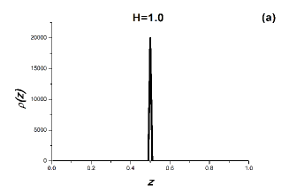
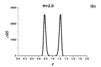
Figure 3: The density distribution at $H=1$ (a) and $H=2$ (b).

Fig. 4 shows several isotherms of the system with $H=1.0$. One can observe several peculiarities along these isotherms, which are marked with labels PT1, …, PT5. Such peculiarities mean that phase transitions are highly likely at these densities. Below we study these phase transitions and identify all phases present in the system.

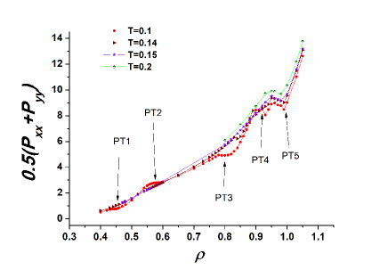
Figure 4: Isotherms of the system in the pore with $H=1$. Labels PT1,…,PT5 show the peculiarities of the equation of state which signalize the appearance of phase transitions.

The first phase transition (PT1) is crystallization of low-density liquid into a triangular crystal. Figs. 5 (a) and (b) show the rdf and the diffraction pattern of the system at $T=0.1$ and $\rho=0.5$. From these figures one can clearly see that the system is in triangular phase at this point.

Figs. 6 (a) and (b) show the rdf of the system at $T=0.1$ and $\rho=0.65$. The system is in a liquid state at this point. It means that reentrant melting takes place in the system.

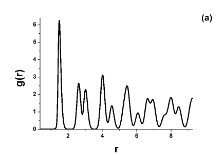
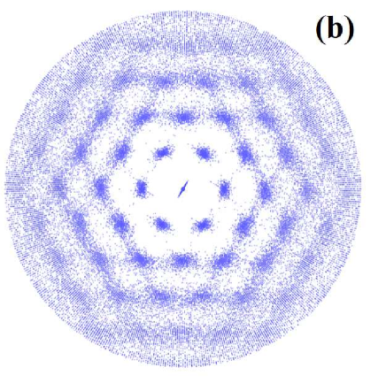
Figure 5: (a) The radial distribution function of the system with $H=1.0$ at $\rho=0.5$ and $T=0.1$; (b) the diffraction pattern of the same system.

Further densification of the system leads to the appearance of a square crystal (PT3). Figs. 7 (a) and (b) show the rdfs and diffraction patterns at $\rho=0.85$. The next phase transition transforms the square crystal into a dodecagonal quasicrystal (see Fig. 8 for the rdfs and diffraction patterns). Finally at high densities the system transforms into a triangular crystal (see Fig. 9 for the rdfs and diffraction patterns). This sequence of phases is analogous to the purely two-dimensional system studied in our previous publications we1 ; we2 ; we3 ; we4 ; we5 .

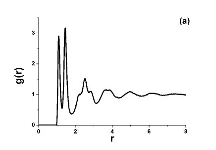
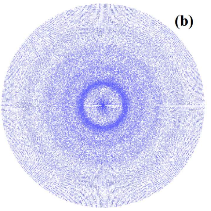
Figure 6: (a) The radial distribution function of the system with $H=1.0$ at $\rho=0.65$ and $T=0.1$; (b) the diffraction pattern of the same system.

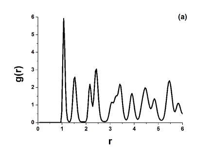
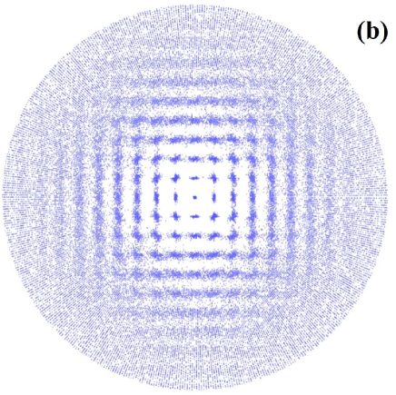
Figure 7: (a) The radial distribution function of the system with $H=1.0$ at $\rho=0.85$ and $T=0.1$; (b) the diffraction pattern of the same system.

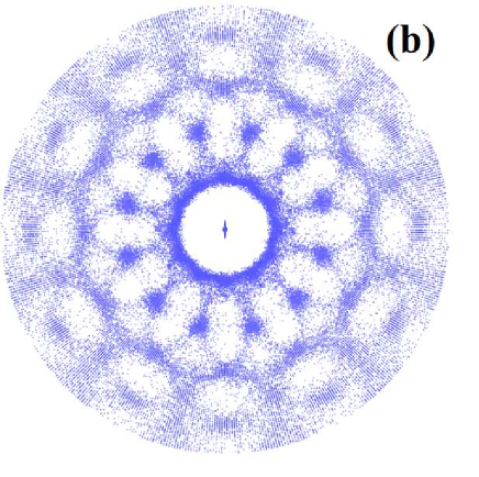
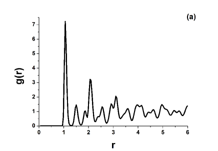
Figure 8: (a) The radial distribution function of the system with $H=1.0$ at $\rho=0.93$ and $T=0.1$; (b) the diffraction pattern of the same system.

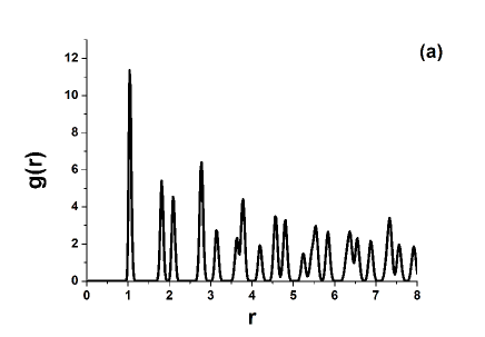
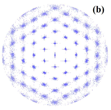
Figure 9: (a) The radial distribution function of the system with $H=1.0$ at $\rho=1.05$ and $T=0.1$; (b) the diffraction pattern of the same system.

Having identified all structures in the system we studied their limits of stability and melting scenarios. First we considered the low density triangular phase and its melting. Similar to the case of the purely $2D$ system this phase demonstrated a maximum on the melting line. Below we will call the branch of the melting line with $\rho<\rho_{max}$ ($\rho_{max}$ is the density of the melting line maximum) a left branch and the one with $\rho>\rho_{max}$ – a right branch. As we discussed in the Introduction, in the case of the purely $2D$ system the melting scenarios for the left and right branches are different: at the left branch a first-order transition takes place, while at the right branch melting occurs in accordance with the third scenario. The water-like anomalies were also found.

Fig. 10 shows the equation of state along several isotherms crossing the stability region of the low density triangular crystal. One can see that two sets of loops appear on these isotherms, which correspond to the crystallization of low density liquid and reentrant melting of the crystal. Since the Mayer-Wood loops are present in the system, both branches demonstrate first order phase transition, i.e. melting should be either first order transition, or the third scenario. In order to determine the transition scenario we consider the correlation functions of the orientational and translational order parameters.

Figs. 11 (a) and (b) show the correlation functions of OOP (a) and TOP (b) at $T=0.1$ crossing the left branch of the melting line. Comparing the densities of the Mayer-Wood loop existence region with the stability limits of the crystal and hexatic phase obtained from correlation function behavior we conclude that at the left branch of the low density phase diagram melting occurs through a single first order phase transition because both stability limits are located within the Mayer-Wood loop existence region.

Figs. 12 (a) and (b) present the same correlation functions at the right branch of the melting line. From comparison of the stability limits obtained from the correlation functions with the position of the Mayer-Wood loop we conclude that at the right branch of the low density phase diagram melting occurs in accordance with the third scenario because the crystal’s stability limit goes beyond the Mayer-Wood loop existence region.

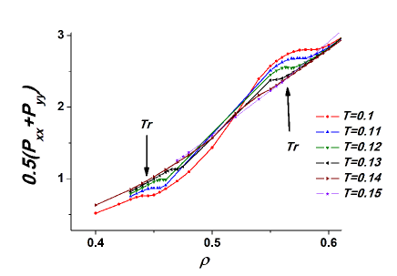
Figure 10: The equation of state along several isotherms crossing the low density triangular phase ($Tr$).

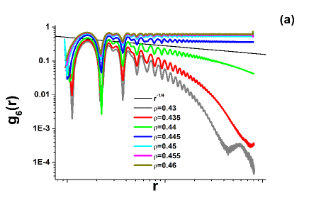
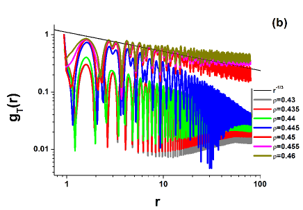
Figure 11: (a) The orientational correlation functions of the system with $H=1.0$ at the left branch of the melting line of the low density triangular crystal at $T=0.1$. (b) The same for the translational correlation functions.

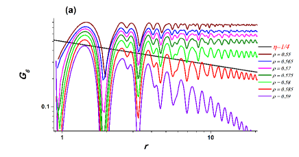
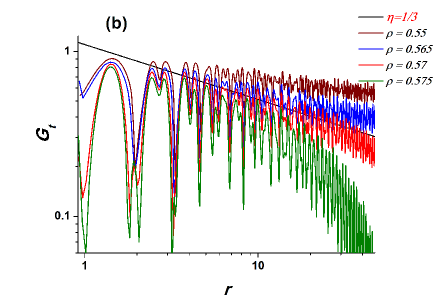
Figure 12: (a) The orientational correlation functions of the system with $H=1.0$ at the right branch of the melting line of the low density triangular crystal at $T=0.1$. (b) The same for the translational correlation functions.

Fig. 13 shows the phase diagrams in the vicinity of the low density triangular crystal for the system with $H=0.3$ and $H=1.0$. In the case of $H=0.3$ the melting lines perfectly coincide with those of the purely $2D$ system (not shown here) ufn1 ; we5 . In the case of $H=1.0$ the qualitative behavior of the system is the same, however, the region of stability of the crystal is shifted to lower temperatures. Thus at a small $H$ the system is strongly confined and out-of-plane motions are negligible. Therefore, the phase diagram coincides with that of the purely $2D$ system. However, at a larger $H$ even if the distribution of density shows a high narrow peak, the out-of-plane motion destabilizes the crystal at lower densities. It is also interesting to note that the temperature of the density anomaly region decreases with an increase in the pore width.

Similar analysis is employed to study the melting lines and coexistence regions of other phases. The phase diagram of the system with $H=1.0$ is shown in Fig. 14, where the phase diagram of the purely $2D$ system is also given for comparison. One can see that at high density the phase diagram of the confined system is in close agreement with that of the purely $2D$ system. Thus one can suppose that at high density the effective strength of confinement appears to be greater, and no strong influence of out-of-plane motion is detected.

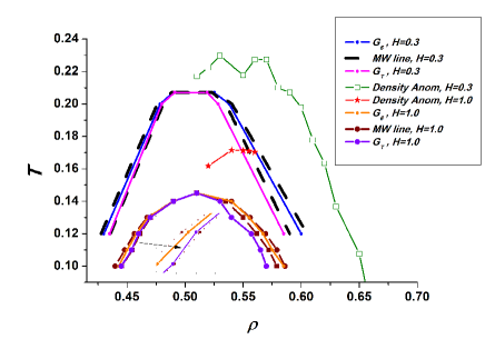
Figure 13: The phase diagrams of the system with $H=0.3$ and $H=1.0$ in the vicinity of the low density triangular crystal. The inset enlarges the part of the left branch of the melting line at $H=1.0$. It enables us to see that a single first order transition preempts the appearance of the hexatic phase in the system. The lines of density anomalies are also shown.

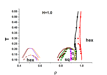
Figure 14: The symbols on the phase diagram of the system with $H=1.0$ in comparison with the phase diagram of the purely $2D$ system (solid lines).

IV Conclusions

In conclusion, we performed a study of the phase diagram of a core-softened system described by the potential (1) Only the case of strong confinement when a single layer of particles is formed is considered. No changes of the phase diagram compared to the purely $2D$ system were detected at very small slit pore width ($H=0.3$). At larger pore width ($H=1.0$) melting of the low density triangular crystal occurred at lower temperatures compared with the purely $2D$ case and the confined system at $H=0.3$ due to intensive out-of-plane motions. The phase diagram at high density remains nearly unaltered regardless of the pore width demonstrating the negligible influence of out-of-plane motions on the melting lines of crystalline phases. These results are in qualitative agreement with the previous studies by other authors rice1 ; rice3 ; rice2 . To provide a fuller picture we plan to perform investigations of confined systems with a wider slit pore, which leads to the appearance of two or more layers.

This work has been carried out using computing resources of the federal collective usage center Complex for Simulation and Data Processing for Mega-science Facilities at NRC ”Kurchatov Institute”, http://ckp.nrcki.ru/, and supercomputers at Joint Supercomputer Center of the Russian Academy of Sciences (JSCC RAS). The work was supported by the Russian Science Foundation (Grant No 19-12-00092).

References

- (1) M. Alcoutlabi and G. B. McKenna, Journal of Physics: Condensed Matter 17, R461 (2005).
- (2) S. A. Rice, Chemical Physics Letters 479, 1 (2009).
- (3) L. B. Krott and M. C. Barbosa, The Journal of Chemical Physics 138, 084505 (2013), https://doi.org/10.1063/1.4792639.
- (4) A. M. Almudallal, S. V. Buldyrev, and I. Saika-Voivod, The Journal of Chemical Physics 137, 034507 (2012), https://doi.org/10.1063/1.4735093.
- (5) R.E. Peierls, Helv. Phys. Acta 7, Suppl. II, 81 (1934).
- (6) R. E. Peierls, Ann. Inst. Henri Poincar e 5, 177 (1935).
- (7) L.D. Landau, Phys. Z. Sowjetunion 11, 26 (1937).
- (8) N. D. Mermin, Phys. Rev. 176, 250 (1968).
- (9) V. L. Berezinskii, Sov. Phys. JETP 32, 493 (1971).
- (10) M. Kosterlitz and D.J. Thouless, J. Phys. C 6 1181 (1973).
- (11) B.I. Halperin and D.R.Nelson, Phys. Rev. Lett. 41 121 (1978).
- (12) D.R.Nelson and B.I. Halperin, Phys. Rev. B 19 2457 (1979).
- (13) A.P. Young, Phys. Rev. B 19 1855 (1979).
- (14) J. M. Kosterlitz, Rep. Prog. Phys. 79, 026001 (2016).
- (15) V. N. Ryzhov, E. E. Tareyeva, Y. D. Fomin and E. N. Tsiok, Phys.-Usp. 60, 857 885 (2017).
- (16) V. N. Ryzhov, Phys.-Usp. 60, 114 (2017).
- (17) K.J. Strandburg, Rev. Mod. Phys. 60, 161 (1988).
- (18) Urs Gasser, C. Eisenmann, G. Maret, and P. Keim, ChemPhysChem 11, 963 (2010).
- (19) K. Zahn and G. Maret, Phys. Rev. Lett. 85 3656 (2000).
- (20) P. Keim, G. Maret, and H.H. von Grunberg, Phys. Rev. E 75, 031402 (2007).
- (21) S. Deutschlander, T. Horn, H. Lowen, G. Maret, and P. Keim, Phys. Rev. Lett. 11, 098301 (2013).
- (22) T. Horn, S. Deutschlander, H. Lowen, G. Maret, and P. Keim, Phys. Rev. E 88, 062305 (2013).
- (23) S.T. Chui, Phys. Rev. B 28, 178 (1983).
- (24) V.N. Ryzhov, Theor. Math. Phys. 88, 990 (1991) (DOI: 10.1007/BF01027701).
- (25) V.N. Ryzhov, Zh. Eksp. Teor. Fiz. 100, 1627 (1991) [Sov. Phys. JETP 73, 899 (1991)].
- (26) V.N. Ryzhov and E.E. Tareyeva, Phys. Rev. B 51 8789 (1995).
- (27) V.N. Ryzhov and E.E. Tareeva, Zh. Eksp. Teor. Fiz. 108, 2044 (1995) [J. Exp. Theor. Phys. 81, 1115 (1995)].
- (28) E.S. Chumakov, Y.D. Fomin, E.L. Shangina, E.E. Tareyeva, E.N. Tsiok, V.N. Ryzhov, Physica A 432, 279 (2015).
- (29) V.N. Ryzhov, E.E. Tareyeva, Yu.D. Fomin, E.N. Tsiok, and E.S. Chumakov, Theoretical and Mathematical Physics 191, 842 (2017) (DOI: 10.1134/S0040577917060058).
- (30) V.N. Ryzhov and E.E. Tareyeva, Physica A 314, 396 (2002).
- (31) V.N. Ryzhov and E.E. Tareyeva, Theor. Math. Phys. 130, 101 (2002) (DOI: 10.1023/A:1013884616321).
- (32) E.P. Bernard and W. Krauth, Phys. Rev. Lett. 107, 155704 (2011).
- (33) M. Engel, J.A. Anderson, S.C. Glotzer, M. Isobe, E.P. Bernard, W. Krauth, Phys. Rev. E 87, 042134 (2013).
- (34) W. Qi, A. P. Gantapara and M. Dijkstra, Soft Matter 10, 5449 (2014).
- (35) S.C. Kapfer and W. Krauth, Phys. Rev. Lett. 114, 035702 (2015).
- (36) A. L. Thorneywork et al, Phys. Rev. Lett. 118, 158001 (2017).
- (37) E. N. Tsiok, Y. D. Fomin, V. N. Ryzhov, Physica A 490, 819 (2018).
- (38) E. A. Gaiduk, Yu.D. Fomin, E. N. Tsiok, V. N. Ryzhov, Molecular Physics (2019) (in press) DOI: 10.1080/00268976.2019.1607917
- (39) M. Zu, J. Liu, H. Tong, and N. Xu, Phys. Rev. Lett. 117, 085702 (2016).
- (40) Yu. D. Fomin, E. A. Gaiduk, E. N. Tsiok, V. N. Ryzhov, Molecular Physics, 116, 3258 (2018) DOI: 10.1080/00268976.2018.1464676
- (41) R. Zangi and S. A. Rice, Phys. Rev. E 58, 7529 (1998).
- (42) A. H. Marcus and S. A. Rice, Phys. Rev. E 55, 637 (1997).
- (43) D. Frydel and S. A. Rice, Phys. Rev. E 68 061405 (2003).
- (44) G. Algara-Siller, O. Lehtinen, F. C. Wang, R. R. Nair, U. Kaiser, H. A.Wu, A. K. Geim and I. V. Grigorieva, Nature 519, 443 (2015).
- (45) K. Koga, G. T. Gao, H. Tanaka, and X. C. Zeng, Nature 412, 802 (2001).
- (46) D. Takaiwa, I. Hatano, K. Koga and H. Tanaka, PNAS 105, 39 (2008).
- (47) H. Kyakuno, K. Matsuda and H. Yahiro, J. Chem. Phys. 134, 244501 (2011).
- (48) Y. Nakamura and T. Ohno, Materials Chemistry and Physics 132, 682 (2012).
- (49) Ch. Ghatak and K. G. Ayappa, Phys. Rev. E 64, 051507 (2001).
- (50) Ch. Ghatak and K. G. Ayappa, Colloids and Surfaces A: Physicochemical and Engineering Aspects 205, 111 117 (2002).
- (51) A. Vishnyakov and A. V. Neimark, J. Chem. Phys. 118, 7585 (2003).
- (52) T. Kaneko, T. Mima, K. Yasuoka, Chem. Phys. Lett. 490, 165 171 (2010).
- (53) Y.D. Fomin, N.V. Gribova, V.N. Ryzhov, S.M Stishov, and D. Frenkel, J. Chem. Phys. 129, 064512 (2008).
- (54) N.V. Gribova, Y.D. Fomin, D. Frenkel, and V.N. Ryzhov, Phys. Rev. E 79 051202 (2009).
- (55) L.B. Krott and M.C. Barbosa, J. Chem. Phys., 138 084505 (2013).
- (56) D.E. Dudalov, Yu.D. Fomin, E.N. Tsiok, and V.N. Ryzhov, Journal of Physics: Conference Series 510, 012016 (2014).
- (57) D. E. Dudalov, E. N. Tsiok, Yu. D. Fomin, and V. N. Ryzhov, J. Chem. Phys. 141, 18C522 (2014).
- (58) E. N. Tsiok, D. E. Dudalov, Yu. D. Fomin, and V. N. Ryzhov, Phys. Rev. E 92, 032110 (2015).
- (59) D.E. Dudalov, Yu.D. Fomin, E.N. Tsiok, and V.N. Ryzhov, Soft Matter 10, 4966 (2014).
- (60) N. P. Kryuchkov, S. O. Yurchenko, Yu. D. Fomin, E. N. Tsiok, and V. N. Ryzhov, Soft Matter 14, 2152 (2018).
- (61) http://lammps.sandia.gov/