Non-convex optimization via strongly convex majoirziation-minimization

Abstract.

In this paper, we introduce a class of nonsmooth nonconvex least square optimization problem using convex analysis tools and we propose to use the iterative minimization-majorization (MM) algorithm on a convex set with initializer away from the origin to find an optimal point for the optimization problem. For this, first we use an approach to construct a class of convex majorizers which approximate the value of non-convex cost function on a convex set. The convergence of the iterative algorithm is guaranteed when the initial point $x^{(0)}$ is away from the origin and the iterative points $x^{(k)}$ are obtained in a ball centred at $x^{(k-1)}$ with small radius. The algorithm converges to a stationary point of cost function when the surregators are strongly convex. For the class of our optimization problems, the proposed penalizer of the cost function is the difference of $\ell_{1}$-norm and the Moreau envelope of a convex function, and it is a generalization of GMC non-separable penalty function previously introduced by Ivan Selesnick in [11].

Keywords: Cost function, local majorizer and minimizer, surregator, Moreau envelope, infimal convolution, convex function, stationary point

MSC2010: 65K05, 65K10, 26B25, 90C26, 90C30

1. introduction

Consider the following optimization problem

(1.1) $$\min_{x\in{\mathcal{C}}}F(x)$$

where ${\mathcal{C}}$ is a closed convex subset of $\mathbb{R}^{N}$ and $F:\mathbb{R}^{N}\to\mathbb{R}$ is a real valued objective or cost function. In general $F$ is continuous but not convex nor smooth. Most optimization problems rely heavily on convexity condition of the function $F$ and the lack of convexity for $F$ makes it usually an NP hard problem to find a global minimum point for the optimization problem (1.1). The convexity condition is in particular useful in some practical problems such as in image reconstruction and sparse recovery. In the absence of the convexity condition, majorization-minimization (MM) algorithm has been proved to be a useful tool in finding local minimization vectors or signals. This algorithm is an iterative algorithm and it converts a difficult optimization problem into a simple one, as we will demonstrate some cases in this paper.

The goal of this paper is for given $y\in\mathbb{R}^{M}$ to solve the following class of least square problems

(1.2) $$\operatorname*{arg\,min}_{x\in\mathbb{R}^{N}}F(x),\quad\text{where}\ \ F(x)=\cfrac{1}{2}\|y-Ax\|_{2}^{2}+\lambda(\|x\|_{1}-f_{\alpha}(x)),\quad\forall x\in\mathbb{R}^{N},$$

using an iterative algorithm. Here, $f_{\alpha}$ is the Moreau envelope of a convex function as defined in (2.3), and $\alpha>0,\lambda>0$ are constants and predetermined. $A\in\mathbb{R}^{M}\times\mathbb{R}^{N}$ is a low rank wide matrix (e.g. a finite frame or wavelet). In our setting, we use tools from convex analysis to introduce the new class of non-convex penalties:

(1.3) $$\psi_{\lambda}(x)=\lambda(\|x\|_{1}-f_{\alpha}(x)).$$

The optimization problem (1.2) is a nonconvex nonsmooth optimization problems subject to the penalty $\psi_{\lambda}(x)$. The cost function $F$ given by (1.2) is in general nonconvex nonsmooth. However, the convexity can hold under some conditions depending on $A$, $\lambda$ and $\alpha$. Note that the main idea of using such nonconvex penalty functions is to promote the sparsity of the solutions in (1.2). A non-convex penalty can induce a nonconvex cost function, thus unnecessary suboptimal local minimizers for the cost function. The main goal of the present paper is twofold. First we introduce a class of functions which majorize the cost function locally. Then we use these majorizers (surrogaters) in an MM algorithm to solve the optimization problem (1.2) and prove that the iteration points convergence to the stationary point of the objective function under some sufficient condition. Before we explain the main contributions of the current work in details, let us first recall some known and special cases of (1.2).

Special cases. When $\lambda=0$, the problem is alternately referred to as minimizer of the residual sum of squared errors (RSS). The solution for minimization can be obtained by least square method. In this case, the minimization is continuously differentiable unconstrained convex optimization problem. For a solution of this case, see e.g. ([6]). When $f_{\alpha}$ is a constant function (which happens in our case, for example, when $\alpha=0$), the problem turns into the classical $\ell_{1}$ regularizer case. This case among the cases with convex regularizer (or penalty term) is more effective in inducing sparse solutions for (1.1) and (1.2) ([2]). However, the $\ell_{1}$ regularizer underestimates the high amplitude components of the solution. The least square problem with an $\ell_{1}$ penalty is known as Least Absolute Selection and Shrinkage Operator (LASSO) ([13]) and Basis Pursuit Denoising ([12]), respectively. Several methods have been introduced in [13, 12] for optimizing the problem. When $f(x)=\|x\|_{1}$, the Moreau envelope $f_{\alpha}$ is the well-known Huber function. The Huber function and its general form as regulizers of sparse recovery problems have been treated in [11], and it has been proved that with these regularizers, using proximal algorithms, the problem (1.2) has an optimal solution provided that $F$ is convex. In this case, the penalty term (1.3) is called GMC penalty.

Main contribution. The first contribution of this paper is to construct a class of convex functions which majorize (surrogate) the cost function $F$ (1.2) locally. We obtain these functions by constructing local minimizers for the penalty term $\psi_{\lambda}$. The local majorizers are tangent to the cost function only at one point and each has a global minimum. The existence of a global minimum for the majorizers is obtained by convexity of majorizers, which we also study here.

The second contribution of this paper is to use the MM algorithm to find a sequence of iteration points which converges to the local minimum of the cost function (1.2). In this algorithm, the initial point $x^{(0)}$ is taken away from zero and each iteration point $x^{(k)}$ is obtained by local minimization of surregator function $F^{M}(\cdot,x^{(k-1)})$ in some small neighbourhood of $x^{(k-1)}$. We prove that the sequence $\{x^{(k)}\}_{k}$ has an accumulation point and it is a stationary point for the cost function $F$ in (1.2), provided that the majorizers are $a$-strongly convex.

Outline. The paper is organized as follows. After introducing some notations and preliminaries in Section 2, in Section 3 we introduce a class of minimizer functions for the penalty term (1.3) and obtain majorizers for the cost function $F$ (1.2). In this section, we also study sufficient conditions for the majorizers to be convex. These results are collected in Lemma 3.1 and Theorem 3.2. In Section 4 we propose to use the iterative MM algorithm with initial point away from zero to guarantee the convergence of iteration points to a stationary point of $F$. These results are collected in Proposition 4.1, Theorem 4.4 and Corollary 4.5.

1.1. Related work

The current paper is proposing the use of majorization-minimization (MM) algorithm to solve the class of nonconvex nonsmooth optimization problems of type (1.2). This approach has been used for example in [5, 7, 9] for solving some optimization problems different than what we consider here. There are another types of methods that have been proved effective in solving nonconvex problems. For example, iteratively reweighted least squares (IRLS) method ([4]) and iteratively reweighted $\ell_{1}$ (IRL1) ([3]). For a list of other methods, we refer the reader to see [9] and the reference therein.

1.2. Acknowledgement

The author wishes to thank Prof. Ivan Selesnick for several insightful discussions and for introducing her the MM algorithm.

2. preliminaries and notations

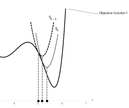
Figure 1. The MM algorithm procedure. The points represent the iteration points $x^{(k-1)},x^{(k)},x^{(k+1)}$.

For any vector $x\in\mathbb{R}^{N}$, the $\ell_{1}$ and $\ell_{2}$ norms of $x$ are defined by $\|x\|_{1}=\sum_{i}|x_{i}|$ and $\|x\|_{2}^{2}=\sum_{i}|x_{i}|^{2}$. By $A\in\mathbb{R}^{M}\times\mathbb{R}^{N}$ we denote the matrix of dimension $M\times N$ and we say it is semindefinite positive and denote it by $A\succeq 0$ if for all $x\in\mathbb{R}^{N}$, $\langle Ax,x\rangle\geq 0$. Here, $\langle\ ,\ \rangle$ denotes the inner product of two vectors. The positive definite is also equivalent to say that all eigenvalues of $A$ are non-negative.

Local majorizers and minimizers: Given a fixed point $w\in\mathbb{R}^{N}$, a function $g(\cdot,w):\mathbb{R}^{N}\to\mathbb{R}$ is called a local majorizer of an objective function $f:\mathbb{R}^{N}\to\mathbb{R}$ at $w$ if the following conditions hold:

(2.1) $$f(x) \leq g(x,w)\quad\forall x\in\mathbb{R}^{N},$$

$$f(x) =g(x,w)\quad\text{if and only if }x=w.$$

The functions $f$ and $g(\cdot,w)$ are tangent at the point $w$ when $f$ and $g(\cdot,w)$ both have directional derivatives at $w$ and for any direction $d\in\mathbb{R}^{N}$ with small $\|d\|_{2}$,

$$\nabla g(w;d,w)=\nabla f_{\alpha}(w;d).$$

From the point of view of geometry, a majorizer means that the surface obtained by the map $x\mapsto g(x,w)$ lies above the surface generated by $x\mapsto f(x)$ and these two surfaces are touching and have tangent point only at $x=w$.

We say a function $g(\cdot,w):\mathbb{R}^{N}\to\mathbb{R}$ minorizes the function $f$ at $w$ when $-g(\cdot,w):\mathbb{R}^{N}\to\mathbb{R}$ majorizes $-f$ at $w$.

Iterative MM algorithm. In minimization algorithm, we choose the majorizer $g_{k-1}:=g(\cdot,x^{(k-1)})$ tangent to objective function at $x^{(k-1)}$ and minimize it on a convex set $\mathcal{D}$ to obtain next iteration point $x^{(k)}$. That is $x^{(k)}:=\operatorname*{arg\,min}_{x\in\mathcal{D}}g(x,x^{(k-1)})$, provided that $x^{(k)}$ exists. We define $g_{k}:=g(\cdot,x^{(k)})$ (see Figure  1).

When the minmization points $x^{(k)}$ exists, the following descending property holds:

(2.2) $$f(x^{(k)})\leq g_{k-1}(x^{(k)})=g(x^{(k)},x^{(k-1)})\leq g_{k-1}(x^{(k-1)})=g(x^{(k-1)},x^{(k-1)})=f(x^{(k-1)}).$$

One of the significant properties of the MM algorithm is its stability due to the descending property of the objective function $f$ (2.2). If an objective function is strictly convex, then the MM algorithm will converge to the unique optimal point (global minimum), assuming that it exists. In the absence of convexity, all stationary points are isolated, then the MM algorithm will converge to one of them. For a complete philosophy of the MM algorithm, we refer the reader, for example, to [8, 7].

Moreau envelope. For a function $\tilde{f}:\mathbb{R}^{N}\to\mathbb{R}$ and $\alpha>0$, the Moreau envelope of the function $\tilde{f}$ is denoted by $f_{\alpha}$ and is defined by infimal convolution

(2.3) $$f_{\alpha}(x):=\left(\tilde{f}\small\Box\cfrac{\alpha}{2}\|\cdot\|_{2}^{2}\right)(x)=\inf_{v\in\mathbb{R}^{N}}\{\tilde{f}(v)+\cfrac{\alpha}{2}\|v-x\|_{2}^{2}\},\quad\forall x\in\mathbb{R}^{N}.$$

The function $f_{\alpha}$ is convex when $f$ is convex and it is the infimal convolution of the function $f$ and the map $x\mapsto\cfrac{\alpha}{2}\|x\|_{2}^{2}$. For example, when $\tilde{f}(x)=\|x\|_{1}$, the Moreau envelope $f_{\alpha}:\mathbb{R}^{N}\to\mathbb{R}\cup\{\infty\}$ is well-known (generalized) Hubber function. For the definition of infimal convolution and its other properties see, e.g., [1].

Let $y\in\mathbb{R}^{M}$ be an observed vector data and $A\in\mathbb{R}^{M}\times\mathbb{R}^{N}$ be a matrix, which is usually a wide low rank matrix. The following result for cost functions $F$ given in (1.2) with penalty term $\psi_{\lambda}(x)=\lambda(\|x\|_{1}-f_{\alpha}(x))$ is a mild improvement of Theorem 1 in [11]. In [11], $\psi_{\lambda}$ is the GMC penalty and the Moreau envelope $f_{\alpha}$ is the generalized Huber function.

Theorem 2.1.

The function $F$ is (strictly) convex if the convexity condition

(2.4) $$A^{T}A-\lambda\alpha I\succeq 0,$$

holds. For strictly convex the inequality $\succeq 0$ is replaced by $\succ 0$. Here, $I$ is the identity matrix.

The proof of this theorem can be obtained by a similar technique which was used to prove Theorem 1 in [11]. Note that the condition (2.4) ensures the uniqueness of the minimizer of cost function $F$.

The convexity condition (2.4) indicates that all eigenvalues of matrix $A^{T}A$ must be at least $\lambda\alpha$. In the absence of convexity condition (2.4), the function $F$ is as sum of a concave function with a convex function and may not be convex, and therefore it may not have any local minimum. In this case, one needs an approach to prove the existence of a global minimum or global optimum point for $F$. This paper proposes the use of MM algorithm technique to solve the minimization problem for $F$, when $F$ is nonconvex.

To reach our goal and prove the existence of a local minimizer for nonconvex objective (or cost) function $F$ (1.2), we first construct local minimizers for the Moreau envelope $f_{\alpha}$, and then use them to obtain local majorizers for $F$. Let $\gamma_{m}>0$ be a constant to be determined later. For any $w\in\mathbb{R}^{N}$, let

(2.5) $$f_{\alpha}^{m}(x,w):=f_{\alpha}(x)-\gamma_{m}\|x-w\|_{2}^{2}.$$

We define $F^{M}(\cdot,w)$ by replacing $f_{\alpha}$ by $f_{\alpha}^{m}(x,w)$ in the definition of the objective function $F$ (1.2) as follows:

(2.6) $$F^{M}(x,w):=\cfrac{1}{2}\|y-Ax\|_{2}^{2}+\lambda\left(\|x\|_{1}-f_{\alpha}^{m}(x,w)\right).$$

It is obvious that for all $x\in\mathbb{R}^{N}$, $F^{M}(x,w)\geq F(x)$. In Theorem 3.2 we prove that the surface generated by the function $F^{M}(\cdot,w)$ is lying about the surface generated by the function $F$ and they touch only at one point $x=w$.

Remark 2.2.

In the same fashion, one can define minorizers $F^{m}(x,w)$ for $F$. For this, let $\gamma_{M}>0$ and define $f_{\alpha}^{M}(x,w):=f_{\alpha}(x)+\gamma_{M}\|x-w\|_{2}^{2}$. Then $f_{\alpha}^{M}(x,w)\geq f_{\alpha}(x)$ for all $x$. Define

$$F^{m}(x,w):=\cfrac{1}{2}\|y-Ax\|_{2}^{2}+\lambda\left(\|x\|_{1}-f_{\alpha}^{M}(x,w)\right).$$

With a similar techniques of proofs for majorizers in the rest of the present paper, one can obtain local minorizers for the cost function $F$ with tangential point at $w$. This is a useful tool in finding local maximums of an optimization problem.

3. Construction of a local majorizer for cost function

Our first result in this section proves the existence of local minorizers for the Moearu envelope function $f_{\alpha}$.

Lemma 3.1 (Minorizer of $f_{\alpha}$).

Fix $w\in\mathbb{R}^{n}$ and define $f_{\alpha}^{m}(\cdot,w)$ as in (2.5). $f_{\alpha}^{m}(\cdot,w)$ is a minorizer for $f_{\alpha}$, and for any direction $d\in\mathbb{R}^{N}$ with $\|d\|_{2}$ small, we have

(3.1) $$\nabla f_{\alpha}(w;d)=\nabla f_{\alpha}^{m}(w;d,w).$$

Proof.

The proof of the local miniorizers for $f_{\alpha}$ is obtained directly from the definition of $f^{m}(\cdot,w)$. To prove (3.1), let $d\in\mathbb{R}^{N}$ with $\|d\|_{2}$ small. Then

(3.2) $$\nabla f_{\alpha}^{m}(w;d,w) =\liminf_{\theta\to 0^{+}}\frac{f_{\alpha}^{m}(w+\theta d,w)-f_{\alpha}^{m}(w,w)}{\theta}$$

$$=\liminf_{\theta\to 0^{+}}\frac{f_{\alpha}^{m}(w+\theta d,w)-f_{\alpha}(w)}{\theta}$$

$$=\liminf_{\theta\to 0^{+}}\frac{\left(f_{\alpha}(w+\theta d)-\gamma_{m}\|\theta d\|_{2}^{2}\right)-f_{\alpha}(w)}{\theta}$$

$$=\liminf_{\theta\to 0^{+}}\frac{\left(f_{\alpha}(w+\theta d)-f_{\alpha}(w)\right)-\gamma_{m}\|\theta d\|_{2}^{2}}{\theta}$$

$$=\liminf_{\theta\to 0^{+}}\frac{\left(f_{\alpha}(w+\theta d)-f_{\alpha}(w)\right)}{\theta}-\liminf_{\theta\to 0^{+}}\gamma_{m}\theta\|d\|_{2}^{2}$$

$$=\liminf_{\theta\to 0^{+}}\frac{\left(f_{\alpha}(w+\theta d)-f_{\alpha}(w)\right)}{\theta}$$

$$=\nabla f_{\alpha}(w;d).$$

This completes the proof of the theorem. ∎

Our next result illustrates that the local minorizers of the Moreau envelope function $f_{\alpha}$ induce local majorizers for $F$.

Theorem 3.2.

The function $F^{M}(\cdot,w)$ (2.6) is local majorizer for the cost function $F$ at $w$, and we have

• $\nabla F(w;d)=\nabla F^{m}(w;d,w)$ for all $d$ with $\|d\|_{2}$ sufficiently small.

• $F^{M}(\cdot,w)$ is (strictly) convex if

  (3.3) $$A^{T}A+\lambda(2\gamma_{m}-\alpha)I\succeq 0.$$

Proof.

By Proposition 3.1 it is immediate that the function $F^{M}(\cdot,w)$ is a local majorizer for $F$. The item (i) also holds by (3.1). To prove the item (ii), we will adapt an approach used to prove Theorem 1 in [11].

Notice the discrepancy with respect to the data in the surregator function $F^{M}(\cdot,w)$ can be written as

(3.4) $$F^{M}(x,w)=x^{T}\left(\frac{1}{2}A^{T}A+\lambda(\gamma_{m}-\frac{\alpha}{2})I\right)x+\lambda\|x\|_{1}+\max_{v\in\mathbb{R}^{N}}g(v,x,w).$$

Notice the function $Q(x):=\max_{v\in\mathbb{R}^{N}}g(v,x,w)$ is not affine although for any fixed $(v,w)$, the map $x\to g(v,x,w)$ is an affine (or linear) function. However, the convexity of $Q$ can be obtained as a result of Proposition 8.14 in [1], since $Q$ is pointwise maximum of convex functions. Therefore by (3.4), $F^{M}(\cdot,w)$ is convex when the quadratic part is convex. This means when the matrix $A^{T}A+\lambda(2\gamma_{m}-\alpha)I$ is positive definite and this completes the proof of (ii). The majorizer function is strictly convex when the inequality is strict. ∎

4. MM algorithm and stationary points

In this section, we prove the existence of a sequence of iteration points which are obtained by minimizing surregator functions at each iteration step. Under strongly convexity condition for the surregators we show that the iteration points have a convergent subsequence and the limit point is a stationary point of $F$. The stationary point is local minimum for $F$ by the descending property (2.2). To prove the existence of the sequence, we continue as follows. First we introduce a notation. For $\epsilon>0$ and $u\in\mathbb{R}^{N}$, we denote by $B_{\epsilon}(u)$ the ball of radius $\epsilon$ with respect to the $\ell_{2}$ norm with center $u$. That is, the set of all points $x\in\mathbb{R}^{N}$ with $\ell_{2}$ norm distance from the center $u$ less than $\epsilon$.

Proposition 4.1.

Let $\alpha>0$ and $\epsilon>0$. Then the sequence obtained by the following iterative algorithm converges.

Set $\gamma_{m}$ such that the convexity condition (3.3) holds;

Initialize $x^{(0)}\in\mathbb{R}^{N}$ such that $\|x^{(0)}\|_{2}>2\epsilon$;

for $k=0,\cdots,$ do

       $x^{(k+1)}=\operatorname*{arg\,min}_{x\in B_{\frac{\varepsilon}{2^{k}}}(x^{(k)})}F^{M}(x,x^{(k)})$;

      

end for

where $k$ is the iteration counter.

Proof.

To prove the proposition, first we claim that the sequence $\{x^{(k)}\}_{k}$ has a convergent subsequence. Then we show that the sequence $\{x^{(k)}\}_{k}$ is that subsequence.

(Boundedness) The iteration points $x^{(k)}$ satisfy

(4.1) $$\|x^{(k+1)}-x^{(k)}\|_{2}\leq\frac{\varepsilon}{2^{k}},\ \ \forall k\geq 0.$$

Using this, iteratively one can show that for any $k$

(4.2) $$0<\|x^{(0)}\|_{2}-\varepsilon\leq\|x^{(k)}\|_{2}.$$

Indeed, the the left side of (4.4) is a positive constant since the initial point $x^{(0)}$ is chosen such that $0<\varepsilon<\frac{\|x^{(0)}\|_{2}}{2}$. From the other hand, the relation (4.1) implies that the sequence is also bounded above. Therefore, by The Bolzano-Weierstrass Theorem the $\{x^{(k)}\}_{k}$ has a convergent subsequence with accumulation point $x^{\ast}$. In what follows we prove that the sequence $\{x^{(k)}\}_{k}$ converges to $x^{\ast}$.

(Convergence) Assume $\{x^{(k_{n})}\}_{n}$ be a subsequence of $\{x^{(k)}\}_{k}$ such that $x^{(k_{n})}\to x^{*}$ as $k_{n}\to\infty$. Fix $k$ and let $k_{n}>k$. An easy calculation shows that

$$\|x^{(k)}-x^{*}\|\leq\|x^{(k_{n})}-x^{\ast}\|+\mathcal{O}(\frac{\epsilon}{2^{k_{n}}})\quad\text{as}\ k\to\infty.$$

This implies that $x^{\ast}$ is the accumulation point for $\{x^{(k)}\}_{k}$ and we are done. ∎

Notice the limit point may not be a stationary (local minimum) point. However, this can be obtained under some sufficient assumptions on the majorizers. First we have a lemma.

Lemma 4.2.

Let $a>0$ and $w\in\mathbb{R}^{N}$. The local majorizer $F^{M}(\cdot,w)$ is $a$-strongly convex provided that $A^{T}A+\lambda(\gamma_{m}-\alpha)I\succeq 2aI$.

Proof.

Recall the discrepancy of data given in (3.4)

$$F^{M}(x,w)=x^{T}\left(\frac{1}{2}A^{T}A+\lambda(\gamma_{m}-\frac{\alpha}{2})I\right)x+\lambda\|x\|_{1}+\max_{v\in\mathbb{R}^{N}}g(v,x,w).$$

This representation implies that $F_{k}^{M}$ is $a$-strongly convex when

(4.3) $$\frac{1}{2}A^{T}A+\lambda(\gamma_{m}-\frac{\alpha}{2})I\succeq al,$$

and we are done. ∎

Strong convexity is one of the most important tools in optimization and in particular it guarantees linear convergence rate of many gradient decent based algorithms. Here, we recall a result:

Lemma 4.3 ([10], Lemma B.5).

Let $f$ be an $a$-strongly convex on a convex domain $\mathcal{D}$. Let $x^{*}$ be the minimizer of $f$ on $\mathcal{D}$. Then

$$a\|x-x^{*}\|_{2}^{2}\leq f(x)-f(x^{*})\quad\forall x\in\mathcal{D}.$$

As an outcome of the lemma we prove that the limit point $x^{*}$ in Theorem 4.1 is a stationary point (thus a local minimizer) for $F$:

Theorem 4.4.

Assume that $a$-strongly convexity condition (4.3) hold, and $\{x^{(k)}\}$ converges to $x^{\ast}$. Then $x^{\ast}$ is a stationary point for $F$ and we have $\nabla F(x^{\ast};d)\geq 0$.

Proof.

For all $x\in\mathbb{R}^{N}$, $f_{\alpha}^{m}(x,x^{(k)})\to f_{\alpha}(x)-\gamma_{m}\|x-x^{\ast}\|_{2}^{2}$ as $k\to\infty$. Thus, $F_{k}^{M}(x)\to F(x)+\lambda\gamma_{m}\|x-x^{\ast}\|_{2}^{2}$, $k\to\infty$. From the other side, by applying Lemma 4.3 to $F_{k}^{M}$ and using the majorization property of this function we obtain

$$a\|x-x^{(k+1)}\|_{2}^{2}\leq F^{M}(x,x^{(k)})-F^{M}(x^{(k+1)},x^{(k)})\leq F^{M}(x,x^{(k)})-F(x^{(k+1)})\quad\forall x\in\mathbb{R}^{N}.$$

So,

$$a\|x-x^{(k+1)}\|_{2}^{2}\leq F^{M}(x,x^{(k)})-F(x^{(k+1)})\quad\forall x\in\mathbb{R}^{N}.$$

By the continuity of $F$, by letting $k\to\infty$ in the preceding inequality, we obtain

$$a\|x-x^{\ast}\|_{2}^{2}\leq F(x)+\lambda\gamma_{m}\|x-x^{\ast}\|_{2}^{2}-F(x^{\ast}),$$

or equivalently

(4.4) $$F(x)-F(x^{\ast})\geq(a-\lambda\gamma_{m})\|x-x^{\ast}\|_{2}^{2}.$$

Let $d\in\mathbb{R}^{N}$ be a direction with $\|d\|_{2}\leq\epsilon$ and $\theta>0$. By (4.4),

$$F(x^{\ast}+\theta d)-F(x^{\ast})\geq(a-\lambda\gamma_{m})\theta^{2}\|d\|_{2}^{2}.$$

This implies that

$$\nabla F(x^{\ast};d)=\liminf_{\theta\to 0^{+}}\cfrac{F(x^{\ast}+\theta d)-F(x^{\ast})}{\theta}\geq(a-\lambda\gamma_{m})\|d\|_{2}^{2}(\liminf_{\theta\to 0^{+}}\theta)=0,$$

and we are done. ∎

The following result is a summary of the results presented in this and previous sections.

Corollary 4.5 (Convergence).

Assume that the local majorizers $\{F^{M}(\cdot,x^{(k)})\}_{k}$ of $F$ are $a$-strongly convex. The sequence of iteration points $\{x^{(k)}\}$ converges and the limit point is a local minimizer of $F$.

Proof.

By Theorem 4.4, $\nabla F(x^{\ast};d)\geq 0$, thus $x^{\ast}$ is an stationary point. By the descending property (2.2), the stationary point is a local minimum. ∎

We conclude this section by illustrating some examples. First we have a notation. For a given matrix $A$, we denote by $\Sigma(A)$ the set of all singular values of matrix $A$.

Example 4.6 (Tight frame).

Assume that the rows of matrix $A$ form a tight frame with frame constant $C$. Then $A^{T}A=CI$ and $\Sigma(A):=\{C\}$. (When $C=1$, the rows of matrix $A$ form a normalized tight frame, also known as Parseval frame.) Let $\alpha$ and $\lambda$ are given such that $\alpha>C\lambda^{-1}$. Then the sufficient convexity condition (2.4) fails for $F$ and the function $F$ may have no local minimum.

In the following example we present a positive lower bound for $\gamma_{m}$ for which the convexity condition (3.3) holds for the majorizers.

Example 4.7.

Assume that the convexity condition (2.4) fails. Thus, for some $\sigma\in\Sigma(A)$ we must have $\alpha>\frac{\sigma}{\lambda}$. This implies that for smallest singular value $\sigma_{0}$ we also have $\alpha>\frac{\sigma_{0}}{\lambda}$. Define $c:=\frac{\lambda\alpha-\sigma_{0}}{2\lambda}$. The constant $c$ is positive and with a straightforward computation one can show that for all pairs $(\gamma_{m},a)$ satisfying

$$\gamma_{m}\geq\frac{a}{\lambda}+c$$

the $a$-strong convexity condition holds for surregators $F^{M}$. The strict convexity also holds when the inequality is strict.

References

- [1] Heinz H Bauschke and Patrick L Combettes, Convex analysis and monotone operator theory in Hilbert spaces, volume 408., Springer, 2011.
- [2] A. Bruckstein, D. Donoho, and M. Elad. From sparse solutions of systems of equations to sparse modeling of signals and images. SIAM Review, 51(1):34-81, 2009.
- [3] Candes, E.J., Wakin, M.B., Boyd, S. Enhancing sparsity by reweighted minimization. J. Fourier Anal. Appl. 14(5), 877-905 (2008)
- [4] Daubechies, I., DeVore, R., Fornasier,M., Gunturk, C.: Iteratively reweighted least squares minimization for sparse recovery. Commun. Pure Appl. Math. 63(1), 1?38 (2010)
- [5] Figueiredo, M.,Bioucas-Dias, J., Nowak, R., Majorization-minimization algorithms forwavelet-based image restoration. IEEE Trans. Image Process. 16(12), 2980-2991 (2007)
- [6] T. Hastie, R. Tibshirani, and J. H. Friedman, The Elements of Statistical Learning. Springer, August 2001.
- [7] Lange, K., Chi, E.C., Zhou, H., A brief survey of modern optimization for statisticians. Int.Stat.Rev. 82(1), 46-70 (2014)
- [8] K. Lang, Optimization, second edition, Springer, 2004.
- [9] A. Lanza, S. Morigi, I. Selesnick, F. Sgallari, Nonconvex nonsmooth optimization via convex-nonconvex majorization-minimization Numerische Mathematik, Volume 136, Issue 2, pp 343-381, 2017
- [10] J. Mairal, Optimization with first-order surrogate functions, ICML 2013-International Conference on Machine Learning, June 2013, Atlanta, United States. 28, pp.783-791, 2013, JMLR Proceedings.
- [11] Ivan Selesnick, Sparse regularization via convex analysis, IEEE Transactions on Signal Processing, 65(17):4481-4494, September 2017
- [12] Scott Shaobing Chen, David L. Donoho, and Michael A. Saunders, Atomic decomposition by basis pursuit, SIAM Journal on Scientific Computing, 20(1):33-61, 1999.
- [13] R. Tibshirani, Regression shrinkage and selection via the lasso, Technical report, University of Toronto, 1994