A COMPREHENSIVE AND UNIFORM SAMPLE OF BROAD-LINE ACTIVE GALACTIC NUCLEI FROM THE SDSS DR7

Abstract

A new, complete sample of 14,584 broad-line active galactic nuclei (AGNs) at $z<0.35$ is presented, which are uncovered homogeneously from the complete database of galaxies and quasars observed spectroscopically in the Sloan Digital Sky Survey Seventh Data Release. The stellar continuum is properly removed for each spectrum with significant host absorption line features, and careful analyses of the emission line spectra, particularly in the H$\alpha$ and H$\beta$ wavebands, are carried out. The broad Balmer emission line, particularly H$\alpha$, is used to indicate the presence of an AGN. The broad H$\alpha$ lines have luminosities in a range of $10^{38.5}$ – $10^{44.3}$ erg s^-1, and line widths (FWHMs) of 500–34,000 $\mathrm{km~{}s^{-1}}$. The virial black hole masses, estimated from the broad-line measurements, span a range of $10^{5.1}$ – $10^{10.3}$ $M_{\odot}$, and the Eddington ratios vary from $-3.3$ to $1.3$ in logarithmic scale. Other quantities such as multiwavelength photometric properties and flags denoting peculiar line profiles are also included in this catalog. We describe the construction of this catalog and briefly discuss its properties. The catalog is publicly available online. This homogeneously selected AGN catalog, along with the accurately measured spectral parameters, provides the most updated, largest AGN sample data, which will enable further comprehensive investigations of the properties of the AGN population in the low-redshift universe.

1 INTRODUCTION

Active galactic nuclei (AGNs) refer to a class of energetic phenomena at the central region of galaxies, which are believed to be powered by the accretion of galactic material onto supermassive black holes (SMBHs). Ever since the recognition of AGNs, including Seyfert galaxies (Seyfert, 1943) and quasars (Schmidt, 1963), AGNs have become one of the most actively studied topics in the astronomy community (e.g, Peterson, 1997; Osterbrock & Ferland, 2006; Netzer, 2013), and enormous effort has been put into compiling large samples of AGNs. Large and uniformly selected samples not only allow systematic and detailed studies on the phenomenological properties of AGNs, but also can yield important insights into the intrinsic physical picture of central black holes (BHs) as well as their surrounding galactic environments. In addition, it is suggested that most BH mass is accumulated during the luminous AGN phases (e.g., Soltan, 1982; Yu & Tremaine, 2002; Merloni, 2004; Shankar et al., 2009). Therefore a complete census of the AGN population and its properties is particularly important to disentangle the BH growth puzzle. In particular, large and well-defined samples can help to measure the luminosity function and the BH mass function of AGNs, as well as the distribution function of the accretion rates, which are useful tools to investigate the AGN demographics and can further provide essential constraints on the growth history of SMBHs (e.g., Schulze et al., 2015). Furthermore, the fact that SMBH mass correlates tightly with the mass, luminosity, and velocity dispersion of the host bulge (e.g., Magorrian et al., 1998; Ferrarese & Merritt, 2000; Gebhardt et al., 2000; Gültekin et al., 2009), indicates that there exists a connection between the growth of SMBHs and the evolution of their host galaxies. This is also supported by semianalytical and numerical simulations on how AGN feedback influences the galaxy formation and evolution (e.g., Di Matteo et al., 2005; Springel et al., 2005; Cattaneo et al., 2006; Croton et al., 2006; Khalatyan et al., 2008; Booth & Schaye, 2009). Large datasets of AGNs, which will drastically extend the physical parameter space of the SMBHs (e.g., BH mass, Eddington ratio, spin) and their host galaxies (ecoevolution.g., morphology, stellar population, distance, and luminosity), can offer unique opportunities to investigate the coevolution between SMBHs and their host galaxies.

In general, AGNs present observational characteristics different from those of stars and normal galaxies, which leads to various methods to search for AGNs. Particularly, optical photometric and spectroscopic observations are efficient in compiling large AGN samples. As a common practice, color selection in the optical band is often used to search for quasar candidates (e.g., Schmidt & Green, 1983; Boyle et al., 1990) and followed by spectroscopical observations, which are essential for identifying their AGN nature and further investigating their properties in detail. Systematic study on a well-defined broad-line AGN sample based on optical spectroscopy was pioneered by Boroson & Green (1992), on the basis of a sample of 87 AGNs with redshifts $z<0.5$ from the Bright Quasar Survey (Green et al., 1986). Recent progress on large samples of quasars is largely attributed to large-scale optical wide-field surveys such as the Sloan Digital Sky Survey (SDSS; York et al., 2000). The SDSS has opened a new frontier in the study of AGNs by providing a huge volume of high-quality spectra of quasars and galaxies. The SDSS makes it feasible to select and study in large and homogeneous AGN samples. A quasar catalog selected from the SDSS DR7 (DR7Q; Schneider et al., 2010) contains 105,783 spectroscopically confirmed quasars, which are luminous AGNs ($M_{i}<−22.0$) that exhibit at least one emission line with FWHM $>1000$ $\mathrm{km~{}s^{-1}}$, or present complex absorption features. Shen et al. (2011) conducted spectral measurements around the H$\alpha$, H$\beta$, Mg II, and C IV regions for DR7Q and estimated the BH masses using various calibrations. A latest SDSS quasar catalog (DR14Q; Pâris et al., 2018) derived from the extended Baryon Oscillation Spectroscopic Survey (eBOSS) of the SDSS-IV has enlarged the number of known quasars to 526,356.

Many studies were also performed focusing on selecting AGNs that are fainter than typical quasars, namely, the so-called Seyfert galaxies. The optical spectra of these underluminous AGNs are generally contaminated by host starlight, thus properly modeling and subtracting the stellar components are essential to detect the broad-line features of AGNs. To achieve this goal, Hao et al. (2005a) developed a set of eigenspectra with main features of absorption line galaxies utilizing the principal component analysis (PCA; e.g., Yip et al., 2004). They compiled a sample of 1317 low-redshift AGNs with the FWHM of broad H$\alpha$ $>1200$ $\mathrm{km~{}s^{-1}}$ from the SDSS DR2 (Abazajian et al., 2004), which was used to investigate the emission line luminosity function of AGNs, especially at a low-luminosity regime (Hao et al., 2005b). Likewise, the PCA methods were adopted to deal with the AGN spectra with significant starlight in later studies. In an effort to study the relation between AGN luminosity and host properties, Vanden Berk et al. (2006) applied the eigenspectrum templates to the spectral decomposition of AGNs and host galaxies, yielding a sample of 4666 low-luminosity type 1 AGNs with FWHM $>1000$ $\mathrm{km~{}s^{-1}}$ from the SDSS DR3. Using a similar method to deal with the galaxy continuum, Greene & Ho (2007a) built a low-redshift broad-line AGN sample from the SDSS DR4 (Adelman-McCarthy et al., 2006). It includes $\sim$8500 objects at $z<0.352$ and was used to investigate the BH mass function for broad-line active galaxies in the local universe. Their broad-line AGN is defined based on the detection of a broad H$\alpha$ component, and their BH masses can extend to the so-called low-mass black hole (LMBH) regime ($M_{\mathrm{BH}}$ $\sim 10^{6}$ $M_{\odot}$). Stern & Laor (2012) presented a type 1 AGN sample of 3579 objects using the SDSS DR7 (Abazajian et al., 2009), which extended the DR7Q sample to the low-luminosity end. They used an approach similar to that of Hao et al. (2005a) to model the host absorption features and set a threshold on the significance of excess flux in the H$\alpha$ region to ensure reliable detection of the broad H$\alpha$ line. Many other attempts were also made to select various types of AGNs by modeling and subtracting the stellar spectra using different techniques. Zhou et al. (2006) selected $\sim$2000 narrow-line Seyfert 1 galaxies (NLS1s) utilizing the Ensemble Learning Independent Component Analysis technique (EL-ICA; Lu et al., 2006) to decompose the stellar and nuclear components in an accurate way. Using a similar decomposition method, Dong et al. (2012) compiled a sample of 8862 sources at $z<0.35$ from the SDSS DR4, which was further used to uniformly select LMBH AGNs, particularly those with low accretion rates as confirmed by X-ray observations (Yuan et al., 2014). Recently, Oh et al. (2015) identified 1835 new type 1 AGNs with FWHM $>800$ $\mathrm{km~{}s^{-1}}$ featuring weak broad-line regions (BLRs) at $z<0.2$ from the SDSS DR7. They fit the stellar spectrum by directly matching the observed spectrum with stellar templates derived from the Bruzual & Charlot (2003) stellar population synthesis models and the MILES stellar library (Sánchez-Blázquez et al., 2006). Their objects have spectra predominantly exhibiting host stellar features but also with a weak broad H$\alpha$ component.

In previous studies focused on compiling type 1 AGN samples, an operational line width (FWHM $\sim 1000$ $\mathrm{km~{}s^{-1}}$; e.g., Hao et al., 2005a; Schneider et al., 2010; Oh et al., 2015) is often adopted as a demarcation between broad and narrow emission lines. This selection criterion works well for luminous AGNs, as the emission line width dominated by the broad-line region (BLR) are broad enough and thus can effectively exclude those type 2 objects. However, type 1 AGNs in the lower-luminosity and lower-BH-mass regimes would fail to meet the FWHM $>1000$ $\mathrm{km~{}s^{-1}}$ criterion. This is particularly true for LMBHs of which the typical broad-line FWHM is $\sim$1000 $\mathrm{km~{}s^{-1}}$, and the minimum width of their broad H$\alpha$ line can even be $\sim 500$ $\mathrm{km~{}s^{-1}}$ (Dong et al., 2012; Greene & Ho, 2007b; Liu et al., 2018). These LMBHs with weak broad-line features have been confirmed to be bona fide AGNs by their X-ray observations (e.g., Greene & Ho, 2007c; Desroches et al., 2009; Yuan et al., 2014). Hence, broad-line AGN catalogs selected using the FWHM $>1000$ $\mathrm{km~{}s^{-1}}$ criterion would be increasingly incomplete with the decreasing AGN luminosity and BH mass. In this study, we do not simply adopt an arbitrary line width as the cutoff between the broad and narrow lines but select broad-line AGNs based on the robustness of the broad components in the Balmer line regions. Particularly, broad-line AGNs thus selected may be used to systematically explore the low-mass end of the local BH mass function (W.-J. Liu 2020, in preparation).

In this paper, we present a large, uniform and well-defined sample, which includes 14,584 broad-line AGNs from the SDSS DR7 at $z<0.35$. We conducted comprehensive spectral analysis and derived complete results of the spectral parameters (e.g., line width, line luminosity, etc.), along with a compilation of photometric data in a multiwavelength band for each object. As described above, the spectra of galaxies and AGNs in the local universe mostly show stellar absorption features in their continua that are not negligible, thus it is essential to precisely subtract the starlight in order to detect possible broad-line features. To model the host continuum, we apply a set of synthesized galaxy spectral templates built from the library of simple stellar populations (SSP; Bruzual & Charlot, 2003) using the EL-ICA technique developed in our previous work (Lu et al., 2006). The robustness and high efficiency of this technique make it ideal for modeling and extracting the stellar characteristics for large data sets. In addition, in order to obtain accurate emission line measurements, we have developed a series of procedures to deal with the decomposition of the coupled broad and narrow components in the Balmer line regions, which have been applied successfully to the spectral analyses in our previous studies of AGNs using the SDSS data (e.g., Dong et al., 2005, 2008, 2012; Zhou et al., 2006; Liu et al., 2018). The paper is organized as follows. In Section 2, we briefly introduce the characteristics of the SDSS, focusing on those aspects most relevant to our study. The spectral analysis and sample selection are outlined in Section 3. In Section 4, we briefly discuss the sample properties and describe the catalog format, followed by a summary in Section 5. Throughout the paper, we assume a cosmology with $H_{0}=70$ $\mathrm{km~{}s^{-1}}$ Mpc^-1, $\Omega_{m}=0.3$, and $\Omega_{\Lambda}=0.7$.

2 THE SDSS DATA

Here we briefly summarize on the characteristics of the SDSS photometry and spectroscopy in this section, and refer readers to Abazajian et al. (2009) for details. The SDSS is a comprehensive imaging and spectroscopic survey using a dedicated 2.5 m telescope (Gunn et al., 2006) located at Apache Point Observatory to image over 10,000 ${\rm deg^{2}}$ of sky and to perform follow-up spectroscopic observations. The telescope uses two instruments. The first is a wide-field imager (Gunn et al., 1998) with 24 $2048\times 2048$ CCDs at the focal plane with 0.396″ pixel covering the sky in a drift-scan mode in five filters $ugriz$ (Fukugita et al., 1996). For each filter, the effective exposure time is 54.1 s, and 18.75 deg² are imaged per hour. The typical 95% completeness limits of the images are $u$, $g$, $r$, $i$, $z=$ 22.0, 22.2, 22.2, 21.3, 20.5, respectively (Abazajian et al., 2004). The imaging data carried out on moonless and cloudless nights of good seeing (Hogg et al., 2001), are calibrated photometrically (Tucker et al., 2006; Padmanabhan et al., 2008) through a series of standard pipelines. The photometric calibration is uncertain at the $\sim$1% level in $griz$ and $\sim$2% in $u$. After astrometric calibration (Pier et al., 2003), the properties of detected objects including the brightnesses, positions and shapes are measured in detail (Stoughton et al., 2002).

The second is a 640-fiber-fed pair of multiobjects double spectrographs covering the wavelength 3800–9200 Å with a resolution of $\lambda/\Delta\lambda$ varying from 1850 to 2200 with a typical signal-to-noise ratio (S/N) of 10 per pixel for a galaxy near the main sample flux limit. Each optical fiber that feeds the spectrograph subtends a diameter of 3″ on the sky, corresponding to 6.5 kpc at $z=0.1$. The instrumental dispersion is $\sim 69~{}\mathrm{km~{}s^{-1}~{}pixel^{-1}}$. The targets chosen for spectroscopic observations are selected based on their photometric data. Galaxy candidates were usually targeted as resolved sources with $r$-band Petrosian magnitudes $r<17.77$, while luminous red ellipticals were specially selected in color– magnitude space with $r<19.2$ and $r<19.5$, respectively, which produce two deeper galaxy candidate samples: one is an approximately volume-limited sample to $z=0.38$, and the other is a flux-limited sample extending to $z=0.55$ (Eisenstein et al., 2001). Quasar candidates are selected by their nonstellar colors in $ugriz$ broad-band photometry and by their radio emissions (unresolved radio counterparts detected by the FIRST survey). This selection targets quasars with $z<3$ to $i$-band point spread function (PSF) magnitude $i=19.1$ and higher redshift quasars ($3<z<5.5$) to $i=20.2$ (Richards et al., 2002). In addition, targeted quasar candidates include optical counterparts to $ROSAT$-detected X-ray sources (Anderson et al., 2007), and other serendipitous objects when free fibers were available on a plate. These targets are arranged on tiles of radius 1.49^∘, and each tile contains 640 objects. The typical spectroscopic exposures are 15 minutes, and more time will be taken for faint plates in order to reach predefined requirements of S/N, namely, $\rm(S/N)^{2}$¿ 15 per 1.5 Å pixel for stellar objects of fiber magnitude $g=20.2$, $r=20.25$, and $i=19.9$.

The SDSS spectra are well calibrated in wavelength and flux. The flux are calibrated by matching the flux of the spectra of standard stars integrated over the filter curves to their PSF magnitudes (Adelman-McCarthy et al., 2008). The flux calibration is accurate to 4% rms, and the wavelength calibration is good to 2 $\mathrm{km~{}s^{-1}}$. The spectra are classified and redshifts determined by a series of pipelines (Stoughton et al., 2002; SubbaRao et al., 2002). The vast majority of these pipeline-determined redshifts are reliable with an accuracy of 99% for galaxies and slightly lower for quasars.

3 SPECTRAL ANALYSIS

Our aim is to build a complete and well-defined sample of broad-line active galaxies in the local universe, based on the SDSS DR7. The SDSS pipeline has determined the redshift $z$ and the classification for each spectrum, and the accuracy is good enough for this study. We start from the spectra classified as “galaxies” or “quasars” with redshifts below 0.35 to ensure the H$\alpha$ lying within the wavelength coverage range of 3800–9200 Å. This results in a parent sample consisting of 854,664 “galaxies” and 11,638 “quasars.” These spectra are first corrected for the Galactic extinction using the extinction map of Schlegel et al. (1998) and the reddening curve of Fitzpatrick (1999) and are then transformed to the rest frame with the redshifts provided by the SDSS pipeline.

There are two key procedures in the spectral analysis: one is the modeling and subtracting of the host stellar continuum, and the other is the decomposition of the broad and narrow components in the H$\alpha$ and H$\beta$ regions. The aperture diameter of the SDSS fibers that feed the spectrograph is 3″ on the sky, which is in general large enough to include significant starlight from the host galaxy in the spectrum. This is particularly true for AGNs fainter than quasars. In fact, several interesting subclasses of AGNs, for instance, LMBHs (e.g, Liu et al., 2018; Dong et al., 2012; Greene & Ho, 2007b), NLS1s (e.g, Zhou et al., 2006), and partially obscured AGNs (e.g, Dong et al., 2005), all show significant starlight in their optical spectra. Hence careful removal of the stellar continuum is necessary, which is important for the reliable follow-up measurement of emission lines and identification of the broad-line features. For this purpose, we (Lu et al., 2006) have developed a set of starlight templates using the EL-ICA algorithm, which can be used to properly decompose the spectra into stellar and nonstellar nuclear components. The details of the continuum fitting method are described in Section 3.1.

The broad Balmer emission lines always blend with narrow-line components and/or the flanking forbidden lines. Thus it is essential to accurately deblend the broad Balmer lines from the narrow lines. In general, we adopt the technique similar to that described in Dong et al. (2012). The profiles of the narrow lines can easily affect the measurement of broad lines, and this can be particularly significant for those objects with weak broad-line features. Hence the narrow-line profile model is crucial for spectral analysis of those sources at the low-luminosity end. We use several different narrow-line profiles to model narrow H$\alpha$ and H$\beta$, and the fits with the minimum $\chi^{2}$ are adopted as the final result. This is physically reasonable, because the narrow Balmer line, for example, H$\alpha$, can arise from emitting regions with a larger range of critical density and ionization than forbidden lines such as [S II], and hence they may have a different profile other than [S II] (Ho et al., 1997). A detailed account of the spectral-line fitting technique is presented in Section 3.2.

For most of the objects, we employ a two-step iteration procedure: first to model and subtract the continuum and next to fit the emission lines. Then the emission line results are adopted as the initial values of the parameters for the second iteration in order to improve the continuum fitting. The iterations are looped until the fits of both the continuum and the emission-line spectrum are statistically and visually acceptable. For a small fraction of objects (about $\sim$20% in the final sample) showing quasar-like spectra, that is, with negligible starlight contribution and prominent and strongly broadened emission lines, a large part of the continuum and Fe II regions would be masked out as emission line regions using the above s tandard procedure. In addition, the Fe II $\lambda\lambda$ 4434–4684 multiplets are often blended with other broad lines such as H$\gamma$, He II  $\lambda 4686$, and H$\beta$, making it complicated to fit the pseudo-continuum in this region. For them, we fit simultaneously the continuum together with the emission lines, including the Fe II multiplets, and the forbidden and the Balmer lines. These procedures are detailed in the following three absorption line subsections.

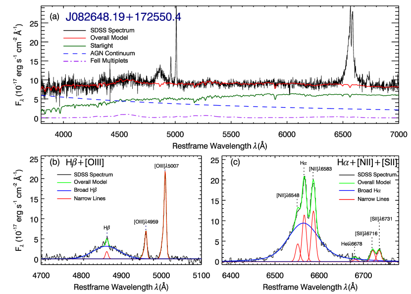
Figure 1: Illustration of the continuum and emission line fitting results for an example of the broad-line AGNs with significant stellar contribution in the spectra. This kind of spectra is dealt with by the two-step iteration procedure as detailed in the text. Panel (a): the observed SDSS spectrum (black), the overall model (red), the decomposed components of the host galaxy (dark green), the AGN continuum (blue dashed), and the Fe II multiplets (purple dotted-dashed). Panel (b): emission line profile fit to the H$\beta$ $+$ [O III] region. Panel (c): emission line profile fit to the H$\alpha$ $+$ [N II] $+$ [S II] region. (The illustration of the continuum and emission-line fits for all the SDSS DR7 broad-line AGNs are available at http://hea.bao.ac.cn/~hyliu/AGN_catalog.html and http://users.ynao.ac.cn/~wjliu/data.html.)

3.1 Starlight and Continuum Subtraction

The vast majority of the parent SDSS sample galaxies ($\sim$99%) have stellar absorption features in their spectra because they are predominately normal galaxies. Hence, proper starlight templates are essential for the continuum fitting. One rough approach is to use the spectra of absorption line galaxies as templates to directly fit the emission-line-free regions of galaxy spectra (e.g., Filippenko & Sargent, 1988). However, it is difficult and time-consuming to find a proper template because the spectra of absorption line and emission line galaxies are quite different. Many attempts have been made to improve the stellar templates in the past decades. PCA is one of these efforts. Hao et al. (2005a) applied the PCA technique to a sample of pure absorption line galaxies and obtained a stellar template library composed of eight eigenspectra. PCA is a statistical method that converts the data into a set of orthogonal and linearly uncorrelated principal components (PCs): the first PC (PC1) contains the maximum variance of the data; PC2 is the second best explanation of the variability of the data and must be orthogonal to PC1; and so forth for each succeeding PC. When applied to stellar template construction, PCA can greatly reduce the number of the galaxy templates but include most of the stellar features in the original galaxy spectra library. This can significantly cut down the computational time cost of the fit and is ideal to deal with large data sets. The ICA algorithm adopted in this study is a blind separation technique that can transform the multidimensional statistical data to a set of statistically independent components (ICs). ICA can be considered as an extension of PCA and inherits its strength of convenience and low time cost in spectral fits. They both attempt to find a set of vectors for the original data so that each point in the data can be described as a linear combination of these vectors. However, ICA is more powerful. PCA requires their PCs to be linearly uncorrelated and orthogonal, while ICA is based on the assumption that the ICs are statistically independent with non-Gaussian distributions but do not need to be orthogonal. Independence is much more concrete than uncorrelatedness, and orthogonality is invalid for a general mixing process. Thus ICA can obtain underlying information from the data when PCA fails. The EL algorithm is a low-cost method that approximates an unknown intractable posterior distribution $p$ by a tractable separable distribution $q$ qualified by a relative entropy $d(q||p)$. EL can be applied to ICA and helps to find the simplest function for the ICs as an interpretation of the data, which thus can greatly mitigate overfit. We (Lu et al., 2006) applied the EL-ICA technique to a library of 1326 stellar spectra spanning a wide range of ages and metallicities (Bruzual & Charlot, 2003), and a set of six nonnegative six ICs, which can explain 97.6% of the 1326 SSP spectra, are chosen as the final galaxy templates. The spectra of these ICs are visually distinctive from each other and imply a tight correlation between stellar population age and the ICs. In general, the galaxy templates constructed using the EL-ICA method can be used to fit a spectrum of any stellar system with a low computational cost and thus are suitable for dealing with large data sets.

As described above, the nuclear emissions from AGNs, especially low-luminosity Seyfert galaxies, are often contaminated by the stellar absorption lines of the host galaxy. Thus before AGN selection, we first model and subtract the stellar continua from the SDSS spectra. A pseudo-continuum model, which takes both the contribution from the host galaxy and the nucleus into account, is adopted to fit the continuum. The so-called pseudo-continuum is a nonnegative linear combination of several properly generated templates, including the stellar component, nuclear continuum, and the optical Fe II multiplets. The Balmer continua and high-order Balmer emission lines are added if they can improve the fit by decreasing the reduced $\chi^{2}$ by at least 20%. The starlight component is modeled by a combination of six synthesized galaxy templates broadened by convolving with a Gaussian of width to match the stellar velocity dispersion of the host galaxy. These synthesized galaxy templates, as detailed above, are built up from the spectral template library of SSPs (Bruzual & Charlot, 2003) using the EL-ICA algorithm (Lu et al., 2006) and have included the vast majority of the stellar features in SSPs and can greatly reduce the chance of overfit. Particularly, we slightly shift the starlight model in adaptive steps to correct for the effect brought by the possible uncertainty of the redshifts provided by the SDSS pipeline, and the fit with the minimum reduced $\chi^{2}$ is adopted as the final result. This can help to measure the host galaxy velocity dispersion and to detect weak emission lines more accurately. A reddened power law of $f(\lambda)\sim\lambda^{-1.7}$ (Francis, 1996), with $E(B-V)$ varying from 0 to 2.5 assuming an extinction curve of the Small Magellanic Cloud (Pei, 1992), is adopted to model the AGN continuum emission. The optical Fe II multiplets are modeled with two separate sets of templates in analytical forms, one for broad lines and the other for narrow lines. These Fe II templates are constructed based on the measurements of I Zw 1 by Véron-Cetty et al. (2004); see Dong et al. (2008, 2011) for details. The merit of the analytical-form Fe II templates is that they enable us to fit the Fe II multiplets with any line width. This is particularly useful in the case of LMBHs, where the spectra tend to show significantly narrower Fe II than those of I Zw 1 (see Greene & Ho, 2007b).

During the pseudo-continuum fitting, two kinds of spectral regions are masked out: (1) bad pixels as flagged by the SDSS pipeline and (2) wavelength ranges emission line that may be seriously affected by prominent emission lines. A composite SDSS quasar spectrum introduced by Vanden Berk et al. (2001) is initially adopted to determine the second mask region. After modeling and subtracting the continuum, the leftover pure emission line spectrum is fitted using the method described in Section 3.2. Then the measured emission line spectrum is used to replace the composite quasar spectrum in the next iteration of the continuum fitting. This two-step procedure is reiterated until that both the continuum and the emission line fitting results are statistically acceptable (either the reduced $\chi^{2}$ $<1.1$ or the fit cannot be significantly improved with a chance probability less than 0.05 according to the $F$-test, $P_{F-{\rm test}}$$<0.05$). An illustration of the starlight-nucleus decomposition is shown in Figure 1.

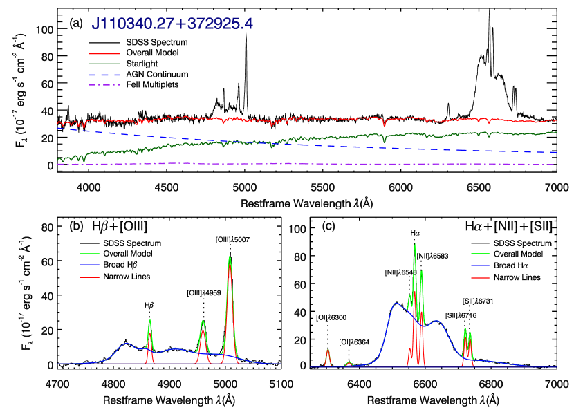
Figure 2: An example of AGNs with complicated broad line profiles. The symbols and lines are the same as those in Figure 1.

3.2 Emission Line Fitting

The emission line fitting procedure adopted in this work is based on and improves upon that used in Dong et al. (2005) and Dong et al. (2012), which is summarized below. We primarily focus on two emission line regions, namely, H$\alpha$ + [N II] (or H$\alpha$ + [N II] + [S II]  if the line width of broad H$\alpha$ is very large) and H$\beta$ + [O III]. The H$\alpha$ + [N II] region is generally complicated because the possible broad H$\alpha$ always blend with the narrow H$\alpha$ and the flanking [N II] doublets. Thus it is necessary to impose some constraints on the narrow lines in order to reduce the number of free parameters. A common approach is to model and fix the profiles of narrow H$\alpha$ and [N II]  using that of [S II], because empirically the line profile of [S II] $\lambda\lambda 6716,6731$ is generally well matched to those of [N II] $\lambda\lambda 6548,6583$ and narrow H$\alpha$. This has been confirmed by Zhou et al. (2006) using a sample of $\sim$3000 type 2 AGNs selected from the SDSS, which shows that both the line widths of both [N II] and [S II] are statistically well consistent with that of narrow H$\alpha$. In some cases, [S II] is undetectable or too weak to yield a reliable measurement, and the [O III] profile is used as a substitute. The [O III] emission lines seem to be significant in almost all the spectra with possible broad-line features. However, they often present an asymmetrical profile and have broad, blue shoulders, which are suggested to originate from outflows. Thus the centroid profile of [O III] $\lambda$5007 is adopted if [O III] is fitted using multiple Gaussians. In general, our fitting strategies for emission lines are as follows:

1. Generally, each narrow line is fitted with a single Gaussian. More Gaussians are added if the [S II] or [O III] doublets show complex profiles and are detected with S/N $>10$ (up to 3 for [O III] and 2 for [S II], respectively). The multi-gaussian scheme is adopted if it improves the fit by $P_{F-{\rm test}}$$<0.05$. The [S II]  doublets are assumed to have the same profile and fixed in separation by their laboratory wavelengths. The same is applied to the [O III] $\lambda\lambda$4959,5007 doublet lines. In addition, the flux ratio of the [O III] doublets $\lambda 5007/\lambda 4959$ is fixed at the theoretical value of 2.98.

2. The narrow H$\alpha$ and [N II] $\lambda\lambda 6548,6583$ are assumed to have the same profiles and redshifts as the [S II] doublets, or the core of [O III] $\lambda\lambda 4959,5007$ if [S II] is absent or weak. The profiles and redshifts of H$\alpha$ and the [N II] doublets are assumed to be the same as [S II] or [O III]. Similar to the [O III]  doublets, the flux ratio of the [N II] doublets $\lambda 6583/\lambda 6548$ is fixed to be 2.96.

3. If the broad H$\beta$ is not detected and the narrow H$\beta$ can be well fitted with one Gaussian, the narrow H$\alpha$ will be given the same profile as the narrow H$\beta$.

4. If the broad and narrow H$\beta$ components cannot be separated by the fit, then the centroid wavelength and profile of the narrow H$\beta$ will be tied to those of H$\alpha$, [O III], or [S II], in this order.

5. The broad H$\alpha$ line is usually fitted using one or two Gaussians, and the broad H$\beta$ is assumed to have the same redshift and profile as the broad H$\alpha$ or set to be free if it can significantly improve the fit of the H$\beta$ + [O III] region by $P_{F-{\rm test}}$$<0.05$. In fact, the line widths of broad H$\beta$ are systematically slightly larger than those of broad H$\alpha$ (e.g., Greene & Ho, 2005), hence the profiles of broad H$\beta$ are set to be free in a moderate fraction of the final broad-line sample. In some spectra, the broad Balmer lines show asymmetric or irregular profiles such as double or even more velocity peaks, and multiple Gaussians (up to 5) are adopted in these cases (see Figure 2).

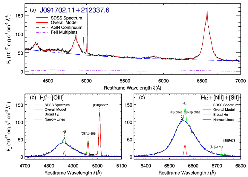
Figure 3: A representative example of AGN spectra without starlight contamination, for which simultaneous fitting of the continuum and emission lines is conducted. Panel (a): the observed SDSS spectrum (black), the overall model (red), the AGN continuum (blue dashed), and the Fe II multiplets (purple dotted-dashed). Panel (b): emission line profile fit to the H$\beta$ $+$ [O III] region. Panel (c): emission line profile fit to the H$\alpha$ $+$ [N II] $+$ [S II] region.

The emission line fitting procedure is composed of three steps. First, we fit the H$\alpha$ + [N II] region using pure narrow-line profiles without a broad component. The narrow H$\alpha$ component and the [N II] $\lambda\lambda 6548,6583$ doublets are modeled and fixed using the [S II], [O III], or narrow H$\beta$, in this order. In the second step, an additional component is added for each spectrum to account for possible broad H$\alpha$ if the $\chi^{2}$ decreases significantly with $P_{F-{\rm test}}$$<0.05$. Thus a subsample of broad-line candidates is selected from the parent sample based on the new added broad H$\alpha$ components that are requested to conform to the criteria that (1) FWHM of the broad component is relatively larger than those of narrow lines, particularly [O III] $\lambda 5007$, and (2) flux of the broad H$\alpha$ is statistically significant, namely, greater than the flux error by a factor of 3, and meanwhile greater than $10^{-16}$ erg s^-1 cm^-2.

Finally, we apply the refined fitting procedure for each candidate broad-line source to improve the accuracy of the line measurement. The profiles of the narrow emission lines in AGNs vary with critical density and ionization parameters. Narrow Balmer lines can arise from emitting regions that may have different physical conditions from those of forbidden-line emitters. Thus the profile of the narrow H$\alpha$ or H$\beta$ may be different from that of [S II] or [O III]. Considering this fact, we employ several different schemes to model the narrow H$\alpha$. The narrow H$\alpha$ is fitted using (1) a model built from the best-fit [S II] with one or double Gaussians; (2) a single-Gaussian model from the best-fit core component of [O III]; (3) a multiple-Gaussian model from the best-fit global profile of [O III]; and (4) a single-Gaussian model built from narrow H$\beta$, if broad H$\beta$ is not detected and narrow H$\beta$ can be fitted well with one Gaussian, respectively. In each scheme, the fitting is constrained following the strategies described above. The fitting results of these different schemes are compared with each other, and the one with the minimum $\chi^{2}$ is adopted as the final result.

3.3 Simultaneous Fit of Continuum and Emission lines

As mentioned above, for objects showing quasar-like spectra, we fit simultaneously the nuclear continuum and the Fe II multiplets, together with other emission lines (see Figure 3). The method is similar to that described in Dong et al. (2008), but with some modifications to improve the accuracy of the measurement of the broad components of H$\alpha$ and H$\beta$, which is described as follows. Each spectrum is fitted in the rest-frame wavelength range of 4200$-$7200 Å using a combination of nuclear continuum, Fe II multiplets, and prominent emission lines in the H$\alpha$ and H$\beta$ regions. The nuclear continuum is modeled by a broken power law with a break wavelength of 5650 Å, for example, $a_{1}\lambda^{-\alpha_{\lambda,1}}$ for the H$\beta$ region and $a_{2}\lambda^{-\alpha_{\lambda,2}}$ for the H$\alpha$ region. The break wavelength of 5650 Å is adopted because it can ideally avoid the wavelength regions of the prominent emission lines based on the AGN composite spectrum given by Vanden Berk et al. (2001). The optical Fe II emission is modeled as $C(\lambda)=c_{b}C_{b}(\lambda)+c_{n}C_{n}(\lambda)$, where $C_{b}(\lambda)$ and $C_{n}(\lambda)$ represent the broad and narrow Fe II line templates in analytical form constructed using the measurements of I Zw 1 provided by Véron-Cetty et al. (2004), as in their Table A1 and A2, respectively. The emission lines other than iron lines are modeled following the strategy described in Section 3.2.

Figure 4: Distributions of the line luminosity, FWHM, EW, and S/N of broad H$\alpha$ line for the present DR7 broad-line AGN sample objects. Contours are local point density contours, and the values of the contour levels are marked for each isoline (the same in the following contour plots).

To ensure the reliability of the line measurements, we recalculate the reduced $\chi^{2}$ of the fits around the H$\alpha$ and the H$\beta$ regions, respectively, and spectra with reduced $\chi^{2}$ $>1.1$ in either region are picked out for further refined fitting. The refined fitting procedures are similar to those described in Section 3.2. Briefly, we fit each pseudo-continuum-subtracted spectrum using various narrow-line models, and the one with the minimum reduced $\chi^{2}$ is adopted. The broad components are fitted using up to five Gaussians; the results are accepted when the reduced $\chi^{2}$ $<1.1$ or it cannot be improved significantly by adding in one more Gaussian with a chance probability $<0.05$ according to the $F$-test.

3.4 Broad-line Selection Criteria

The conventionally broad line criterion of FWHM $\sim 1000$ $\mathrm{km~{}s^{-1}}$ (e.g., Hao et al., 2005a; Schneider et al., 2010; Oh et al., 2015) would inevitably reject a large fraction of type 1 AGNs at the low-mass and low-luminosity end, and hence results in significant incompleteness of the sample. In this work, we adopt the selection criteria following Dong et al. (2012) and Liu et al. (2018), based directly on the presence of a broad component (c.f. the narrow lines) from the results of emission line fitting, particularly, broad H$\alpha$, which is generally the strongest broad line in the optical spectra of AGNs. The criteria are as follows:

1. $P_{F\rm-test}<0.05$,
2. Flux(H$\alpha^{\rm b}$) $>10^{-16}$ erg s^-1 cm^-2,
3. S/N(H$\alpha^{\rm b}$) $\geq 5$,
4. $h_{\rm B}\geq 2$ rms, and
5. FWHM(H$\alpha^{\rm b}$) $>$ FWHM(NL),

where $P_{F{\rm-test}}$ is the chance probability given by the $F$-test and is used to test whether adding a broad H$\alpha$ component in the pure narrow-line model can significantly improve the fit or not; S/N(H$\alpha^{\rm b}$) $=$ Flux(H$\alpha^{\rm b}$)$/\sigma_{\rm total}$, H$\alpha^{\rm b}$ denotes the broad component of H$\alpha$ line, $\sigma_{\rm total}$ is the total uncertainty of broad H$\alpha$ arising from statistical noise, continuum subtraction, and subtraction of nearby narrow lines, as will be elaborated below; $h_{\rm B}$ is the height of the best-fit broad H$\alpha$ component, and rms is the quadratic mean deviation of the continuum-subtracted spectra in the emission-line–free region near H$\alpha$; FWHM is full width at half maximum, and NL refers to narrow line.

Figure 5: Distributions of the line luminosity, FWHM, EW, and S/N of the broad H$\beta$ line for the present DR7 broad-line AGN sample objects.

Criterion 1 gives the statistical significance of detecting a broad H$\alpha$ given by the $F$-test. We have found through simulations that these criteria based on the $F$-test work well, although theoretically, these goodness-of-fit tests hold only for linear models (see Hao et al., 2005a). The flux limit in criterion 2 is set to eliminate possible spurious detections caused by underlying inappropriate continuum subtraction. The broad H$\alpha$ component detected at $10^{-16}$ erg s^-1 cm^-2  appears to be a fake broad feature because a slight fluctuation in the continuum may result in a marginal broad H$\alpha$ detection with such a flux. In fact, even the minimum broad H$\alpha$ flux in our final broad-line AGN sample is much larger than this threshold. Criterion 3 is to ensure the reliability of the existence of the broad component in terms of S/N. S/N(H$\alpha^{\rm b}$) $=$ Flux(H$\alpha^{\rm b}$)$/\sigma_{\rm total}$, and $\sigma_{\rm total}$ is the quadrature sum of statistical noise ($\sigma_{\rm stat}$), the uncertainties arising from the subtraction of continuum ($\sigma_{\rm cont\_sub}$) and narrow lines ($\sigma_{\rm NL\_sub}$), namely, $\sigma^{2}_{\rm total}=\sigma^{2}_{\rm stat}+\sigma^{2}_{\rm NL\_sub}+\sigma^{2}_{\rm cont\_sub}$ . The $\sigma_{\rm stat}$ is given by the fitting code MPFIT. The significance of the $\sigma_{\rm NL\_sub}$ depends on the width and intensity of the broad H$\alpha$ line. In cases where broad H$\alpha$ are broad and strong, the decomposition between broad and narrow lines is apparent and has little influence on the measured flux of broad H$\alpha$; this term is small and negligible. However, for a broad H$\alpha$ line that is both narrow and weak, this term may be significant, because the line deblending is highly dependent on the narrow-line model. Hence we estimate the $\sigma_{\rm NL\_sub}$ based on fitting results using different narrow models. In the stage of refined fitting for emission lines, we have employed several different narrow-line models to deal with each spectrum. The rest $n$ sets of fitting results that are worse than the best one with a chance probability of the $F$-test greater than 0.1 are selected to estimate the $\sigma_{\rm NL\_sub}$,

$$\footnotesize\sigma_{\rm NL\_sub}=\sqrt{\frac{\sum_{i=1}^{n}({\rm Flux(H\alpha^{\rm b}})_{i}-{\rm Flux(H\alpha^{\rm b})}_{\rm best})^{2}}{n}}~{}.$$ (1)

As for $\sigma_{\rm cont\_sub}$, in practice, this term is difficult to estimate. The H$\alpha$ absorption lines in those spectra with old stellar populations may moderately affect the flux measurements. However, this situation is rare in our final sample. On the whole, we suppose the error term caused by the continuum subtraction is negligible because the H$\alpha$ absorption features are weak in most cases and the flux uncertainty of broad H$\alpha$ introduced by continuum decomposition is much below 1 $\sigma$ (also see the discussion in footnote 12 of Dong et al., 2012). Criterion 4 is a supplementary constraint, which can help to minimize spurious detections mimicked by narrow-line wings or fluctuation in the continuum. In the vast majority of cases, the selected broad-line objects based on the S/N threshold in criterion 3 have $h_{\rm B}$ much larger than 2 rms. Criterion 5 is set to ensure the “broad” feature of the broad component in terms of line width. It requires that the FWHM of the broad H$\alpha$ be larger than those of narrow lines. Our analysis yielded a total of 14,584 sources (with duplicates removed) that pass these criteria.

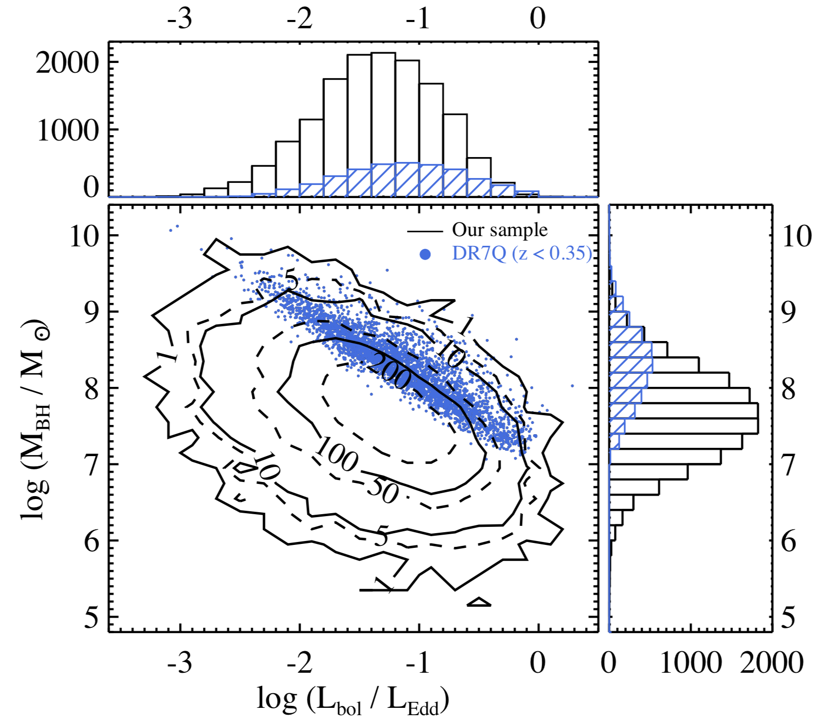
Figure 6: Distributions of the BH mass and Eddington ratio for our broad-line AGN sample (black contour) and the DR7Q sample at $z<0.35$ (blue circles, Schneider et al., 2010; Shen et al., 2011). The deficit of data points at the upper right corner indicates that there exist few fast accreting massive AGNs in the local universe, while the absence of objects at the lower left region is due to the flux limit of the SDSS. The right and top panels show the BH mass and Eddington ratio histograms for our broad-line AGNs (black histograms), respectively. The blue hatched histograms represent the distribution of the DR7Q objects at $z<0.35$. The DR7Q terminates at $M_{\mathrm{BH}}$ $\approx 10^{7}$ $M_{\odot}$, while the BH masses of the broad-line AGNs in our sample span a wide range of $10^{5.1}-10^{10.3}$ $M_{\odot}$.

4 THE SAMPLE

4.1 Sample Properties

We have compiled a sample of 14,584 type 1 AGNs based on detection of a broad H$\alpha$ line from a total of about one million SDSS DR7 spectroscopic objects. The median $z$ of the final broad-line AGN sample is 0.2. The line luminosities, FWHMs, and EWs are measured for the entire sample. The FWHMs are measured from the multi-Gaussian models as described in Section 3.2, and their uncertainties are derived from simulations. Figure 4 and Figure 5 show the distributions of these quantities for broad H$\alpha$ and H$\beta$. The FWHMs of H$\alpha^{\rm b}$ span a range of $\sim$500$-$34000 $\mathrm{km~{}s^{-1}}$, with a median of 2760 $\mathrm{km~{}s^{-1}}$. The broad H$\alpha$ line luminosities $L_{\rm H\alpha^{\rm b}}$ reside in the range of $\sim 10^{38.5}-10^{44.3}$ erg s^-1 with a median lying at $10^{42.1}$ erg s^-1. EWs of broad H$\alpha$ cover a range of $5-900$ Å with a median of 232 Å. For the broad H$\beta$ line, the FWHMs, luminosities, and EWs are located in the range of $\sim 500-$34000 $\mathrm{km~{}s^{-1}}$, $10^{38.9}-10^{43.7}$ erg s^-1, and $\sim 1-780$ Å, respectively; and their medians are 3020 $\mathrm{km~{}s^{-1}}$, $10^{41.5}$ erg s^-1, and 43 Å, respectively. The distributions of the median S/N per pixel around the H$\alpha$ and H$\beta$ regions show that most of the emission line measurements except for line luminosity have no significant dependence on the S/N, which indicates that the selection of broad-line AGNs is unbiased by the S/N of the spectra. As for the dependence of line luminosity on S/N, we consider that it is more likely to be caused by the selection effect due to the SDSS flux limit.

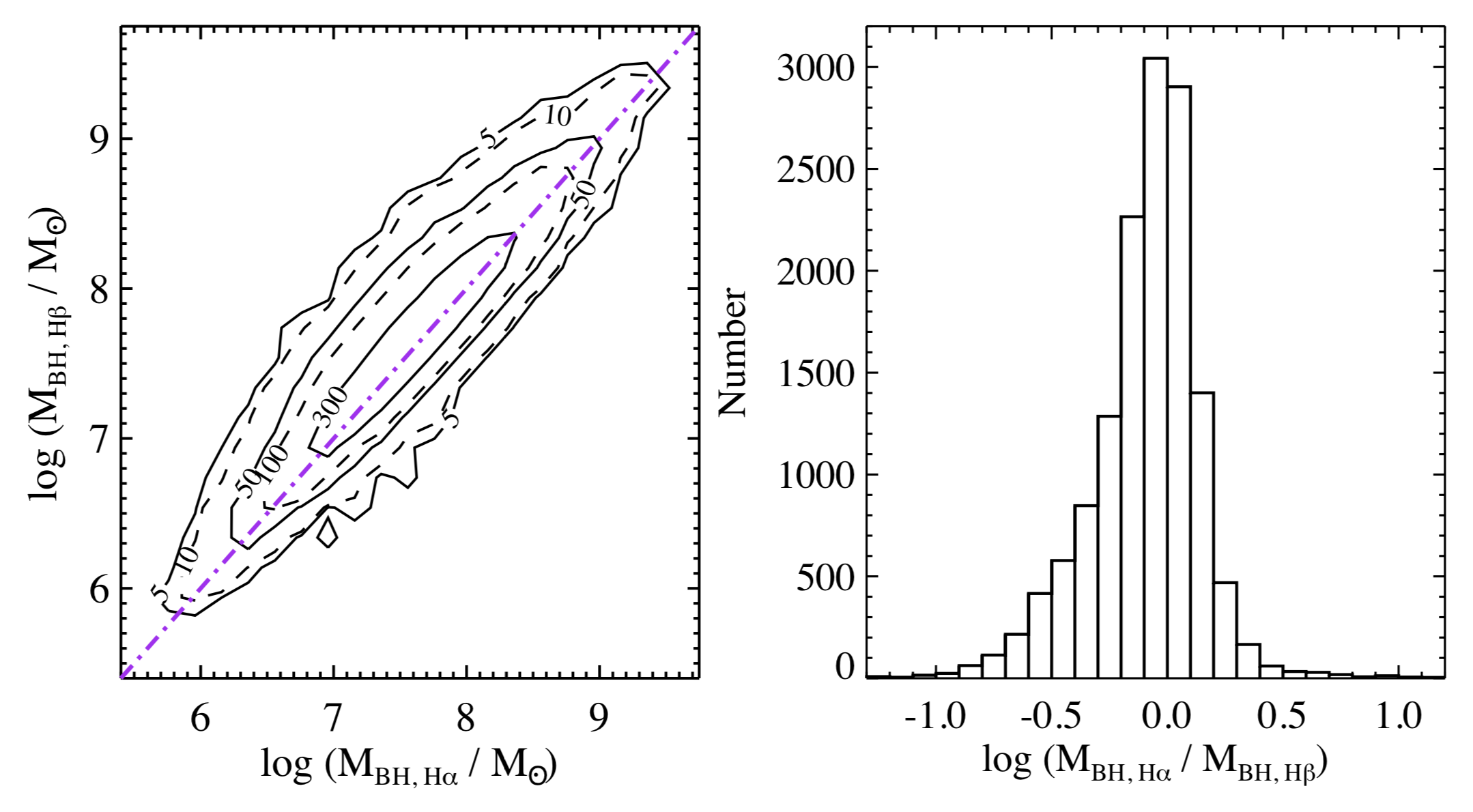
Figure 7: Comparison of virial masses derived from two different line estimators based on the broad H$\alpha$ and H$\beta$ lines, respectively, for our broad-line AGN sample objects of which both line estimates are available. The contour in the left panel presents their distribution on the $M_{\rm BH,H\alpha}$ versus $M_{\rm BH,H\beta}$ space, and the marked values on the isolines are corresponding number densities. The dotted-dashed line denotes 1:1. The right panel shows the distribution of mass ratios between these two lines. The BH masses derived from broad H$\beta$ are slightly larger than those obtained from broad H$\alpha$.

The BH masses can be estimated using the spectral measurements based on the virial method. This method assumes that the BLR system is virialized; the BLR radius is estimated from the continuum luminosity using the radius-luminosity (R-L) relation derived from reverberation mapping (RM) studies of AGNs (e.g., Kaspi et al., 2005; Bentz et al., 2006, 2009, 2013; Wang et al., 2009), and the virial velocity is indicated by the broad-line width (FWHM or line dispersion). The scaling factor depends on the structure of the BLR system and can be calibrated by other BH mass estimators such as $M-\sigma_{*}$ relation (e.g., Ferrarese & Merritt, 2000; Gebhardt et al., 2000). Here we adopt the BH estimator outlined in Ho & Kim (2015), which was calibrated using a larger and more current sample of reverberation mapping AGNs than previous studies and taking into account the recent determination of the virial coefficient for pseudo and classical bulges. This estimator is subject to an intrinsic scatter of 0.35 dex. The $M_{\mathrm{BH}}$ based on broad H$\beta$ are derived as follows:

$$\footnotesize\rm log{\it M}_{BH}=log\left[\left(\frac{FWHM(H\beta)}{1000~{}\mathrm{km~{}s^{-1}}}\right)^{2}\left(\frac{L_{5100}}{10^{44}erg~{}s^{-1}}\right)^{0.533}\right]+6.91,$$ (2)

where $L_{5100}$ is the continuum luminosity at rest frame 5100 Å ($L_{5100}\equiv$ $\lambda L_{\lambda}$(5100 Å)), which is derived from the AGN continua decomposed from the spectra or from the broad H$\beta$/H$\alpha$ luminosity using the scaling relation given in Greene & Ho (2005) if the spectra are dominated by starlight. $M_{\mathrm{BH}}$  are also estimated based on the broad H$\alpha$ using the above formalism and the empirical correlation between FWHM of broad H$\alpha$ and H$\beta$ given by Greene & Ho (2005). The final nominal $M_{\mathrm{BH}}$ for each object is adopted as the mean of $M_{\mathrm{BH}}$(H$\beta$) and $M_{\mathrm{BH}}$(H$\alpha$) whenever both are possible. The BH masses span a range of $10^{5.1}-10^{10.3}$ $M_{\odot}$, with a median of $10^{7.6}$ $M_{\odot}$. The Eddington ratio ($L\mathrm{{}_{bol}}$$/$$L\mathrm{{}_{Edd}}$) is calculated using the measured $L_{5100}$ and the nominal BH masses. It is defined as the ratio of the bolometric luminosity ($L_{\rm bol}$) to the Eddington luminosity ($L\mathrm{{}_{Edd}}=1.26\times 10^{38}M_{\mathrm{BH}}/M_{\odot}$). $L_{\rm bol}$ is derived from the optical continuum luminosity at 5100 Å using a bolometric correction factor of 9.8 (McLure & Dunlop, 2004), $L_{\rm bol}=9.8L_{5100}$. The Eddington ratios thus estimated range from $-$3.3 to 1.3 in logarithmic scale, with a median of $-$1.3. Figure 6 shows the distributions of BH masses and Eddington ratios.

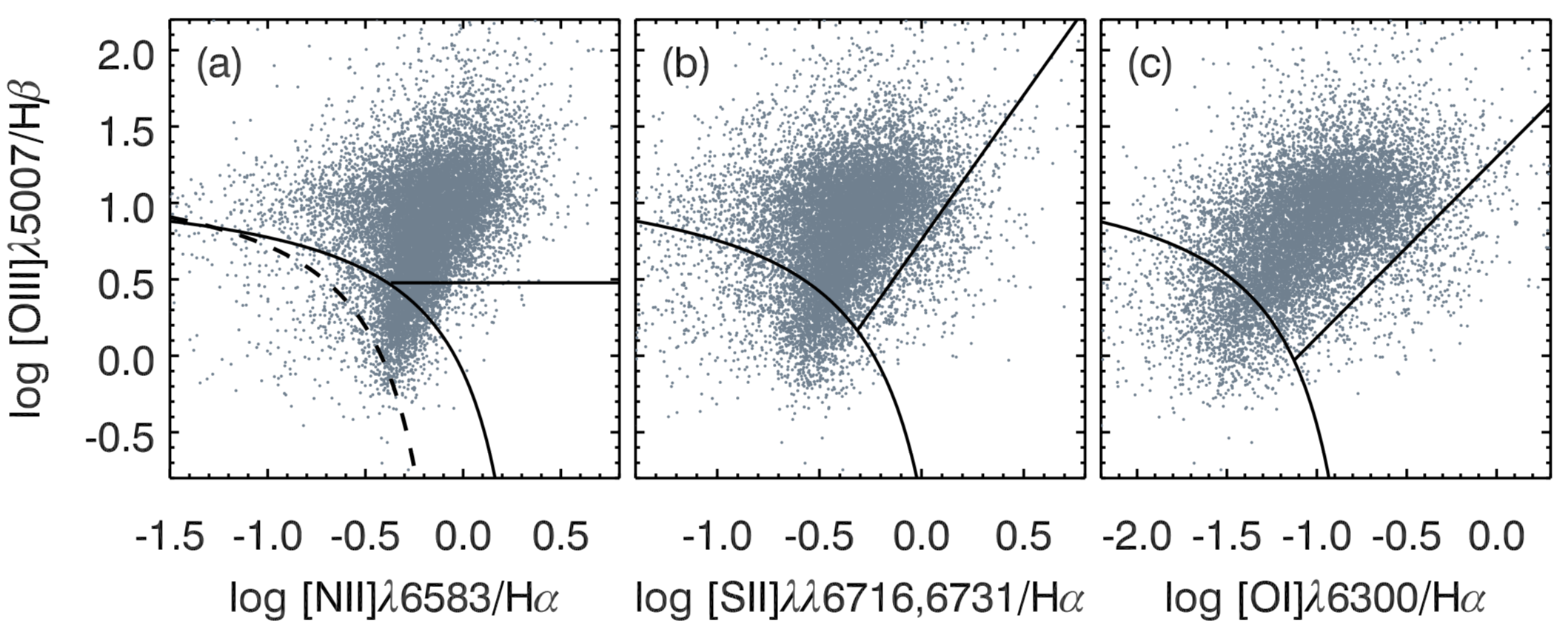
Figure 8: Narrow-line diagnostic diagrams of [O III] $\lambda 5007/$H$\beta$ versus [N II] $\lambda 6583/$H$\alpha$ (a), versus [S II] $\lambda\lambda 6716,6731/$H$\alpha$ (b), and versus [O I] $\lambda 6300/$H$\alpha$ (c) for the broad-line AGN sample in this study. The extreme starburst classification line (solid curve from Kewley et al., 2001 and the Seyfert–LINER line (solid straight line in panel $b$ and $c$) obtained by Kewley et al. (2006) are adopted to separate the H II regions, AGNs and LINERs. In panel ($a$), the dashed line corresponds to the pure star formation line given by Kauffmann et al. (2003), and the horizontal line represents [O III] $\lambda 5007/$H$\beta$ $=3$, which is conventionally used to separate Seyfert galaxies and LINERs.

Figure 7 presents the comparison between the BH masses estimated from H$\alpha$ and H$\beta$. The BH masses derived from broad H$\beta$ are slightly larger than those obtained from broad H$\beta$. The direct reason is that the H$\alpha$-based BH mass formalism is not calibrated independently, but by substituting into the H$\beta$-based BH mass estimator using the empirical FWHM relation between broad H$\alpha$ and broad H$\beta$ (Eq. 3 of Greene & Ho, 2005). The intrinsic mechanism is complicated; in fact, there are a lot of systematics involved in deriving these H$\alpha$- or H$\beta$-based BH masses. For instance, the local R-L relation is biased toward the most variable AGNs (Bentz et al., 2013), thus derived BH mass estimators using single-epoch spectra suffer large uncertainties; the relative profile of H$\alpha$ and H$\beta$ depends on both the kinematic and ionization structure of the BLR (Osterbrock & Ferland, 2006), which can vary quite significantly among different objects; dust extinction can also alter the profile of Balmer emission lines, and the Balmer decrements for the objects in our sample span a wide range. Many ($\sim$68%) are larger than the typical H$\alpha$/H$\beta$ of 3.5 for objects in Greene & Ho (2005).

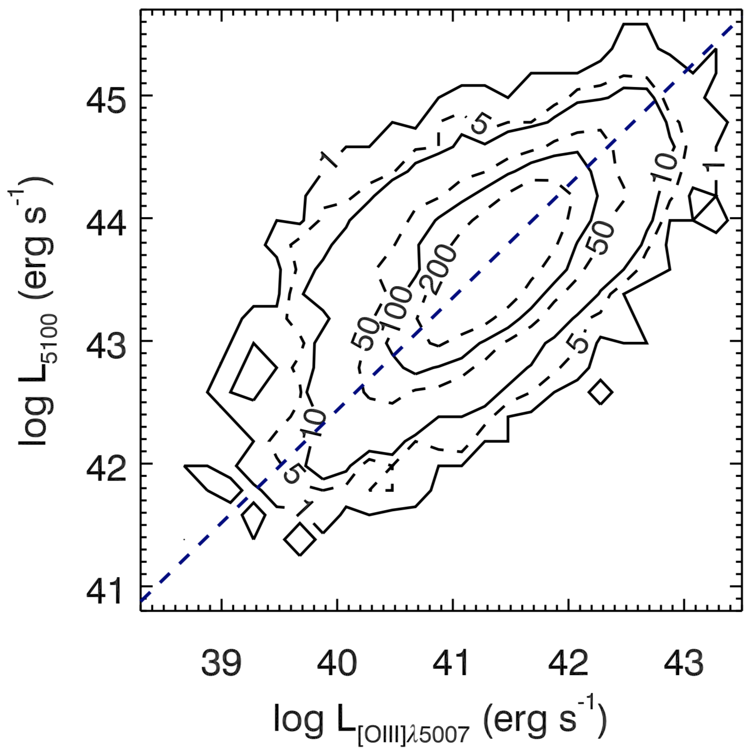
Figure 9: Correlation between the [O III] line luminosity ($L_{\rm[O\,{\footnotesize III}]\,\lambda 5007}$) and the continuum luminosity at 5100 Å ($L_{5100}$). The navy dashed line denotes a bisector linear regression fit described in the text, and the best-fit relation is ${\rm log}(L_{5100})=0.92{\rm log}(L_{\rm[O\,{\footnotesize III}]\,\lambda 5007})+5.76$, with a scatter of $\sim$0.43 dex.

AGNs can also be identified from their loci in the diagnostic diagrams constructed by the relative strengths of various prominent narrow emission lines, namely, so-called BPT diagrams, which are commonly used to select narrow-line AGNs. The BPT diagrams involving the narrow-line ratios of H$\alpha$, H$\beta$, [O III], [N II], [S II], and [O I] are shown in Figure 8. The vast majority of our type 1 AGNs are located in the region of either Seyfert galaxies or composite objects. Only a small fraction (3%) fall into the pure star-forming region, which can be explained by the large aperture of 3″ of the SDSS that inevitably includes light from the host galaxies. This result confirms the AGN nature of our sample. Moreover, the AGN nature was partly verified by the X-ray properties of some of these broad-line objects, which is particularly important, or those showing weak broad-line features such as LMBHs (Yuan et al., 2014; Liu et al., 2018).

Figure 9 shows the correlation between the [O III] $\lambda 5007$ luminosity and the continuum luminosity at 5100 Å. This scaling relation is generally used to estimate the bolometric luminosity using the [O III] $\lambda 5007$ luminosity as a proxy for type 2 AGNs (e.g.,Kauffmann et al., 2003; Heckman et al., 2004; Reyes et al., 2008. However, as noted in previous studies (e.g., Heckman et al., 2004; Reyes et al., 2008), this correlation suffers from a large scatter. The [O III] $\lambda 5007$ line is expected to be affected by interstellar dust extinction and the complicated condition makes it difficult to correct. This would introduce uncertainty in this correlation as well. Here we give a rough linear relation between $L_{\rm[O\,{\footnotesize III}]\,\lambda 5007}$ and $L_{5100}$, namely, ${\rm log}(L_{5100})=0.92{\rm log}(L_{\rm[O\,{\footnotesize III}]\,\lambda 5007})+5.76$, with a scatter of $\sim$0.43 dex.

Figure 10 shows the dependence of the intensity ratio Fe II $\lambda 4570$ to [O III] $\lambda 5007$ ($L_{{\rm Fe\,{\footnotesize II}}\,\lambda 4570}/L_{\rm[O\,{\footnotesize III}]\,\lambda 5007}$) on $L_{5100}$, $M_{\mathrm{BH}}$, $L\mathrm{{}_{bol}}$$/$$L\mathrm{{}_{Edd}}$, which is in the framework of the eigenvector 1 AGN parameter space introduced by Boroson & Green (EV1 or PC1; 1992). The flux of the Fe II $\lambda 4570$ is integrated in the rest-frame wavelength range 4434–4684 Å. EV1 was suggested to be physically driven by the relative accretion rate or the Eddington ratio (e.g., Boroson & Green, 1992; Boroson, 2002). This was confirmed by Dong et al. (2011) utilizing a large, homogenous AGN sample selected from the SDSS, who found that the intensity ratio of Fe II $\lambda 4570$ to [O III] $\lambda 5007$ indeed correlates most strongly with $L\mathrm{{}_{bol}}$$/$$L\mathrm{{}_{Edd}}$, rather than with $M_{\mathrm{BH}}$ or $L_{5100}$. However, in this work, we find that $L_{{\rm Fe\,{\footnotesize II}}\,\lambda 4570}/L_{\rm[O\,{\footnotesize III}]\,\lambda 5007}$ is correlated with both $L_{5100}$ and $L\mathrm{{}_{bol}}$$/$$L\mathrm{{}_{Edd}}$ at similar levels (with Spearman’s rank coefficients of $r_{\rm S}=0.35$, 0.27, and chance probabilities of $p=9\times 10^{-37}$, $5\times 10^{-31}$, respectively). No correlation is found with $M_{\mathrm{BH}}$ ($r_{\rm S}=-0.05$ and $p=0.003$). The physical mechanisms driving these correlations in the parameter space are currently not clear and deserve further study in the future.

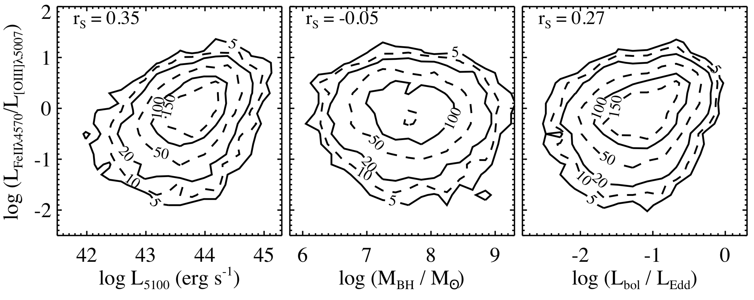
Figure 10: Dependence of the line ratio of Fe II $\lambda 4570$ to [O III] $\lambda 5007$ on the continuum luminosity $L_{5100}$, BH mass ($M_{\mathrm{BH}}$), and Eddington ratio ($L\mathrm{{}_{bol}}$$/$$L\mathrm{{}_{Edd}}$), respectively. Also denoted are the Spearman correlation coefficient $r_{\rm S}$. The relative strength of Fe II $\lambda 4570$ to [O III] $\lambda 5007$ shows moderate dependence on $L_{5100}$ and $L\mathrm{{}_{bol}}$$/$$L\mathrm{{}_{Edd}}$ but no correlation with $M_{\mathrm{BH}}$.

4.2 Comparisons with Other Broad-line AGN Samples

4.2.1 Comparison with the SDSS DR7 quasar sample

The quasar catalog based upon the SDSS DR7 (DR7Q, Schneider et al., 2010; Shen et al., 2011), which contains 105,783 objects with luminosities higher than $M_{i}=-22.0$ and redshifts at $0.065<z<5.46$, was selected using the classical broad-line criterion of FWHM $>1000$ $\mathrm{km~{}s^{-1}}$. It is interesting to compare the current sample with DR7Q because our study adopts a different strategy, which is based directly on the detection of broad Balmer lines for the selection of type 1 AGNs. Figure 11 presents the distributions on the $L_{\rm H\alpha^{\rm b}}$ versus $z$ plane for DR7Q and our sample. The loci of these two samples coincide at $z>0.3$; however, our sample becomes distinct at $z<0.3$ due to the deficit of low-luminosity AGNs in DR7Q. DR7Q includes 3532 objects at $z<0.35$, 3419 out of which are also included in our sample. The right panel in Figure 11 compares the distribution of $L_{\rm H\alpha^{\rm b}}$ spanned by our sample with DR7Q at $z<0.35$. The median $L_{\rm H\alpha^{\rm b}}$ of DR7Q at $z<0.35$ is 42.9 in logarithmic scale, systematically higher than the 42.1 of our sample; in particular, our sample includes 6733 objects at $L_{\rm H\alpha^{\rm b}}$$<10^{42}$ erg s^-1, in sharp contrast with 25 in DR7Q. The distributions of FHWM(H$\alpha^{\rm b}$) for DR7Q at $z<0.35$ and for our sample are generally consistent within 0.06 dex (their medians are 3150 $\mathrm{km~{}s^{-1}}$ and 2760 $\mathrm{km~{}s^{-1}}$, respectively). Furthermore, the DR7Q objects at $z<0.35$ have BH masses spanning from $10^{7.1}$ $M_{\odot}$ to $10^{10.5}$ $M_{\odot}$ with a median of $10^{8.3}$ $M_{\odot}$, while our sample extends down by almost 2 orders in magnitude in $M_{\mathrm{BH}}$ and includes 2154 objects with $M_{\mathrm{BH}}$ below $10^{7}$ $M_{\odot}$ (see Figure 6). In terms of the Eddington ratios, the difference between these two samples is not so significant as in BH mass; the median $L\mathrm{{}_{bol}}/L\mathrm{{}_{Edd}}$ of our sample is about 0.2 dex lower than that of DR7Q ($-$1.35 vs. $-$1.13). In summary, our sample is a good complement to DR7Q, in the sense that it enlarges the number of low-$z$ type 1 AGNs by a factor of 4 (thus more complete) and extends the SDSS AGN sample to the lower-luminosity and lower-BH-mass end.

The present sample, which puts more efforts into finding faint AGNs, provides a large database of local AGNs spanning wide ranges of various quantities, for example, luminosity, line width, BH mass, Eddington ratio, and so on, especially in the low-BH-mass regime. This can help to investigate the properties of AGNs of particular interest such as low-luminosity AGNs with low Eddington ratios (LINERs), active BHs at the lowest-mass regime (LMBHs), and NLS1s that are suggested to be accreting at their Eddington limits. In particular, the LMBHs in this sample can help study the connection between SMBHs and their host galaxies in the low-mass regime, which is poorly explored so far. LMBHs are suggested to be predominately located in pseudobulges, which seem not to follow the correlations between SMBHs and the quantities of classical bulges (e.g, mass, luminosity, velocity dispersion). In addition, being well defined and more complete in the low-BH-mass regime than previous ones, our sample can be used to construct the BH mass function and luminosity function for BHs in the local universe. These studies, especially for AGNs with $M_{\mathrm{BH}}$ $<10^{6}$ $M_{\odot}$, can provide important constraints for models of the formation and evolution of BHs (Greene & Ho, 2007a; Volonteri, 2010).

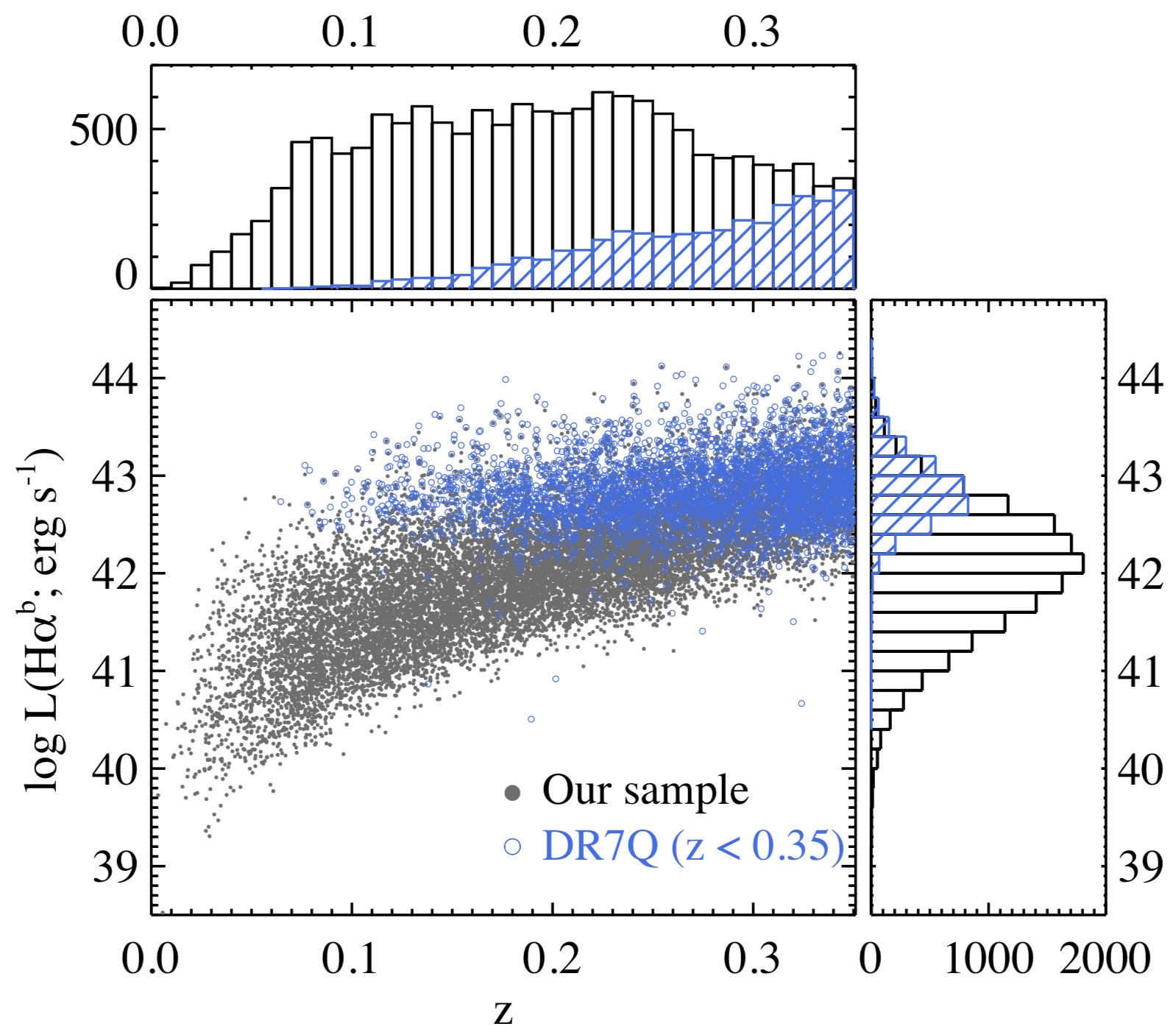
Figure 11: Distributions of type 1 AGNs in this study (gray filled circles) and DR7Q objects at $z<0.35$ (blue open circles) on the $L_{\rm H\alpha^{\rm b}}$ versus $z$ plane. The loci of these two samples overlap at $z>0.3$, and our sample becomes distinct due to the lack of faint AGNs in DR7Q at $z<0.3$. The right and top panels show the luminosity and redshift histograms, respectively. Note that the vast majority of DR7Q objects at $z<0.35$ reside at $L_{\rm H\alpha^{\rm b}}$ $>10^{42}$ erg s^-1, while our sample extends further down to $L_{\rm H\alpha^{\rm b}}$ $\approx 10^{39}$ erg s^-1.

4.2.2 Comparisons with other low-luminosity type 1 AGN samples

Greene & Ho (2007a) constructed a sample of $\sim$8500 broad-line active galaxies (hereafter GH07) from the SDSS DR 4 with redshift $z<0.352$, of which 92% (7839) are included in our sample as well. The broad-line detection rates of GH07 and our samples are comparable; this is not surprising because the broad-line selection strategies of these two samples are similar. The medians of redshift, broad H$\alpha$ luminosity, and FWHM of GH07 sample are 0.2, 42.06, and 2830, respectively, which are similar to those of our sample (the differences are within 0.1 dex). Note that our sample have more objects located in the low-luminosity regime (the fraction of sources with $L_{\rm H\alpha^{\rm b}}$ $<10^{41}$ erg s^-1 in our sample is 8.1% vs. 4.5% of the GH07 sample), which indicates that our approach has the advantage of detecting fainter AGNs with weaker broad H$\alpha$, as demonstrated in Dong et al. (2012) and Liu et al. (2018) as well (LMBH AGN samples).

Stern & Laor (2012) obtained a sample of 3579 type 1 AGNs with $z<0.31$ (hereafter SL12), selected also from the SDSS DR 7 based on the detection of broad H$\alpha$ emission. Their sample objects have a broad H$\alpha$ luminosity of $10^{40}-10^{44}$ erg s^-1 with a median of $10^{42}$ erg s^-1, and a broad H$\alpha$ width (FWHM) of 1000–25000 $\mathrm{km~{}s^{-1}}$ with a median of 3200 $\mathrm{km~{}s^{-1}}$. The vast majority of the objects in the SL12 sample (3468) are included in our sample as well, while we note that the SL12 sample is much smaller than ours. The absence of a large fraction of the broad-line AGNs in our sample in SL12 may be due to their stricter criteria on selecting the broad H$\alpha$line: the FWHM of broad H$\alpha$ larger than 1000 $\mathrm{km~{}s^{-1}}$ and the broad H$\alpha$ flux larger than four times the scatters of the continuum-subtracted spectrum near H$\alpha$. These two further criteria excluded AGNs with narrower or weaker broad lines. In addition, they applied several filters on the DR7 database, which resulted in a substantial decrease in the size of the parent sample.

4.3 Description of the Catalog

We have tabulated the measured quantities from the spectral fitting for the 14,584 broad-line AGNs, along with their photometric data in multiwavelength bands. This catalog is composed of three parts: the first contains the basic information of each object; the second part is the emission line measurements derived from the spectral analysis in this work; the third part is a compilation of the multi-wavelength photometric measurements obtained from other surveys.

Table 1: The SDSS DR7 Broad-line AGN Sample (Part I)

ID	Designation	R.A.	Decl.	$z$	Plate	MJD	FiberID	$N_{\rm spec}$
(1)	(2)	(3)	(4)	(5)	(6)	(7)	(8)	(9)
1	J000048.16$-$095404.0	0.20064719	$-$9.9011221	0.205	650	52143	494	1
2	J000102.19$-$102326.9	0.2591277	$-$10.390799	0.294	650	52143	166	1
3	J000111.15$-$100155.5	0.29645887	$-$10.032093	0.049	650	52143	174	1

Note. — Col. (1): Identification number assigned in this paper. Col. (2): Official SDSS designation in J2000.0. Col. (3): Right ascension in decimal degrees (J2000.0). Col. (4): Declination in decimal degrees (J2000.0). Col. (5): Redshift measured by the SDSS pipeline. Col. (6): Spectroscopic plate number. Col. (7): Modified Julian date (MJD) of spectroscopic observation. Col. (8): Spectroscopic fiber number. Col. (9): Number of spectroscopic observations. (This table is available in its entirety in a machine-readable form in the online journal. A portion is shown here for guidance regarding its form and content.)

4.3.1 Object Information

Part I of the catalog (see Table 1) is composed of the basic information of these sources including the identification number assigned in this paper, the SDSS name, coordinates, redshift, spectroscopic plate, modified Julian date (MJD) and fiberid, together with the number of spectroscopic observations. The objects in this catalog are sorted by their R.A. and Dec, and their redshifts are taken from the SDSS pipeline. Plate is an integer indicating the SDSS plug plate that was used to collect the spectrum; MJD denotes the modified Julian date of the night when the observation was carried out; fiberid denotes the fiber id (1–640 for SDSS DR7). Any given spectrum can be identified by the combination of these three numbers. In the SDSS, spectra for many objects are taken simultaneously, and thus some objects were observed more than once with different plate-MJD-fiberid combinations. For those objects with multiple observations, we adopt the spectrum of the highest median S/N and record the number of spectroscopic observations in the flag $N_{\rm spec}$.

Table 2: Catalog Format for the SDSS DR7 broad-line AGN sample (Part II)

Column	Name	Format	Description
1	ID	LONG	Identification number assigned in this paper.
2	CENTROID_BHA	DOUBLE	Centroid wavelength of broad H$\alpha$ (Å)
3	CENTROID_BHA_ERR	DOUBLE	Uncertainty in Centroid wavelength of broad H$\alpha$ (Å)
4	LBHA	DOUBLE	Line luminosity of broad H$\alpha$ [$\log(L_{{\rm H\alpha,broad}}/\rm erg~{}s^{-1})$]
5	LBHA_ERR	DOUBLE	Uncertainty in $\log L_{{\rm H\alpha,broad}}$
6	FWHM_BHA	DOUBLE	FWHM of broad H$\alpha$ ($\mathrm{km~{}s^{-1}}$)
7	FWHM_BHA_ERR	DOUBLE	Uncertainty in the ${\rm FWHM_{H\alpha,broad}}$
8	EW_BHA	DOUBLE	Restframe equivalent width of broad H$\alpha$ (Å)
9	EW_BHA_ERR	DOUBLE	Uncertainty in ${\rm EW_{H\alpha,broad}}$
10	CENTROID_NHA	DOUBLE	Centroid wavelength of narrow H$\alpha$ (Å)
11	CENTROID_NHA_ERR	DOUBLE	Uncertainty in Centroid wavelength of narrow H$\alpha$ (Å)
12	LNHA	DOUBLE	Line luminosity of narrow H$\alpha$ [$\log(L_{{\rm H\alpha,narrow}}/\rm erg~{}s^{-1})$]
13	LNHA_ERR	DOUBLE	Uncertainty in $\log L_{{\rm H\alpha,narrow}}$
14	FWHM_NHA	DOUBLE	FWHM of narrow H$\alpha$ ($\mathrm{km~{}s^{-1}}$)
15	FWHM_NHA_ERR	DOUBLE	Uncertainty in the ${\rm FWHM_{H\alpha,narrow}}$
16	EW_NHA	DOUBLE	Restframe equivalent width of narrow H$\alpha$ (Å)
17	EW_NHA_ERR	DOUBLE	Uncertainty in ${\rm EW_{H\alpha,narrow}}$
18	LNII6583	DOUBLE	Line luminosity of $\rm[N\,{\footnotesize II}]\lambda$6583 [$\log(L_{{\rm[N\,{\footnotesize II}]\lambda 6583}}/\rm erg~{}s^{-1})$]
19	LNII6583_ERR	DOUBLE	Uncertainty in $\log L_{{\rm[N\,{\footnotesize II}]\lambda 6583}}$
20	EW_NII6583	DOUBLE	Restframe equivalent width of $\rm[N\,{\footnotesize II}]\lambda$6583 (Å)
21	EW_NII6583_ERR	DOUBLE	Uncertainty in ${\rm EW_{[N\,{\footnotesize II}]\lambda 6583}}$
22	LSII6716	DOUBLE	Line luminosity of $\rm[S\,{\footnotesize II}]\lambda$6716 [$\log(L_{{\rm[S\,{\footnotesize II}]\lambda 6716}}/\rm erg~{}s^{-1})$]
23	LSII6716_ERR	DOUBLE	Uncertainty in $\log L_{\rm[S\,{\footnotesize II}]\lambda 6716}$
24	EW_SII6716	DOUBLE	Restframe equivalent width of $\rm[S\,{\footnotesize II}]\lambda$6716 (Å)
25	EW_SII6716_ERR	DOUBLE	Uncertainty in ${\rm EW_{[S\,{\footnotesize II}]\lambda 6716}}$
26	LSII6731	DOUBLE	Line luminosity of $\rm[S\,{\footnotesize II}]\lambda$6731 [$\log(L_{{\rm[S\,{\footnotesize II}]\lambda 6731}}/\rm erg~{}s^{-1})$]
27	LSII6731_ERR	DOUBLE	Uncertainty in $\log L_{\rm[S\,{\footnotesize II}]\lambda 6731}$
28	EW_SII6731	DOUBLE	Restframe equivalent width of $\rm[S\,{\footnotesize II}]\lambda$6731 (Å)
29	EW_SII6731_ERR	DOUBLE	Uncertainty in ${\rm EW_{[S\,{\footnotesize II}]\lambda 6731}}$
30	LOI6300	DOUBLE	Line luminosity of $\rm[O\,{\footnotesize I}]\lambda$6300 [$\log(L_{{\rm[O\,{\footnotesize I}]\lambda 6300}}/\rm erg~{}s^{-1})$]
31	LOI6300_ERR	DOUBLE	Uncertainty in $\log L_{\rm[O\,{\footnotesize I}]\lambda 6300}$
32	EW_OI6300	DOUBLE	Restframe equivalent width of $\rm[O\,{\footnotesize I}]\lambda$6300 (Å)
33	EW_OI6300_ERR	DOUBLE	Uncertainty in ${\rm EW_{[O\,{\footnotesize I}]\lambda 6300}}$
34	Centroid_BHB	DOUBLE	Centroid wavelength of broad H$\beta$ (Å)
35	Centroid_BHB_ERR	DOUBLE	Uncertainty in Centroid wavelength of broad H$\beta$ (Å)
36	LBHB	DOUBLE	Line luminosity of broad H$\beta$ [$\log(L_{{\rm H\beta,broad}}/\rm erg~{}s^{-1})$]
37	LBHB_ERR	DOUBLE	Uncertainty in $\log L_{{\rm H\beta,broad}}$
38	FWHM_BHB	DOUBLE	FWHM of broad H$\beta$ ($\mathrm{km~{}s^{-1}}$)
39	FWHM_BHB_ERR	DOUBLE	Uncertainty in the ${\rm FWHM_{H\beta,broad}}$
40	EW_BHB	DOUBLE	Restframe equivalent width of broad H$\beta$ (Å)
41	EW_BHB_ERR	DOUBLE	Uncertainty in ${\rm EW_{H\beta,broad}}$
42	CENTROID_NHB	DOUBLE	Centroid wavelength of narrow H$\beta$ (Å)
43	LNHB	DOUBLE	Line luminosity of narrow H$\beta$ [$\log(L_{{\rm H\beta,narrow}}/\rm erg~{}s^{-1})$]
44	LNHB_ERR	DOUBLE	Uncertainty in $\log L_{{\rm H\beta,narrow}}$
45	EW_NHB	DOUBLE	Restframe equivalent width of narrow H$\beta$ (Å)
46	EW_NHB_ERR	DOUBLE	Uncertainty in ${\rm EW_{H\beta,narrow}}$
47	CENTROID_OIII5007	DOUBLE	Centroid wavelength of $\rm[O\,{\footnotesize III}]\lambda$5007 (Å)
48	CENTROID_OIII5007_ERR	DOUBLE	Uncertainty in Centroid wavelength of $\rm[O\,{\footnotesize III}]\lambda$5007 (Å)
49	LOIII5007	DOUBLE	Line luminosity of $\rm[O\,{\footnotesize III}]\lambda$5007 [$\log(L_{{\rm[O\,{\footnotesize III}]5007}}/\rm erg~{}s^{-1})$]
50	LOIII5007_ERR	DOUBLE	Uncertainty in $\log L_{\rm[O\,{\footnotesize III}]5007}$
51	FWHM_OIII5007	DOUBLE	FWHM of $\rm[O\,{\footnotesize III}]\lambda$5007 ($\mathrm{km~{}s^{-1}}$)
52	FWHM_OIII5007_ERR	DOUBLE	Uncertainty in the ${\rm FWHM_{[O\,{\footnotesize III}]\lambda 5007}}$
53	EW_OIII5007	DOUBLE	Restframe equivalent width of $\rm[O\,{\footnotesize III}]\lambda$5007 (Å)
54	EW_OIII5007_ERR	DOUBLE	Uncertainty in ${\rm EW_{[O\,{\footnotesize III}]\lambda 5007}}$
55	LFeII4570	DOUBLE	Line luminosity of $\rm{\rm Fe\,{\footnotesize II}}\lambda$4570 [$\log(L_{{\rm{\rm Fe\,{\footnotesize II}}4570}}/\rm erg~{}s^{-1})$]
56	LFeII4570_ERR	DOUBLE	Uncertainty in $\log L_{\rm{\rm Fe\,{\footnotesize II}}4570}$
57	EW_FeII4570	DOUBLE	Restframe equivalent width of $\rm{\rm Fe\,{\footnotesize II}}\lambda$4570 (Å)
58	EW_FeII4570_ERR	DOUBLE	Uncertainty in ${\rm EW_{{\rm Fe\,{\footnotesize II}}\lambda 4570}}$
59	L5100	DOUBLE	Monochromatic luminosity at 5100 Å in log-scale
60	L5100_ERR	DOUBLE	Uncertainty in monochromatic luminosity at 5100 Å in log-scale
61	MultiPeak	Long	0 = no peculiar profile; 1 = $\rm[O\,{\footnotesize III}]\lambda$5007 with multiple peak profile;
			2 = broad Balmer line with multiple peak profile
62	MBH_BHB	DOUBLE	Virial black hole mass in log-scale based on H$\beta$ (Ho & Kim, 2015)
63	MBH_BHA	DOUBLE	Virial black hole mass in log-scale based on H$\alpha$ (derived from Ho & Kim, 2015 and Greene & Ho, 2005)
64	MBH	DOUBLE	The adopted fiducial virial black hole mass in log-scale
65	LAMBDA_EDD	DOUBLE	Eddington ratio based on the fiducial virial BH mass ($\log$ $L\mathrm{{}_{bol}}$/$L\mathrm{{}_{Edd}}$)

Note. — This table is available in its entirety in a machine-readable form in the online journal.

4.3.2 Emission line Measurements

The measured quantities obtained from the spectral analysis in this work are included in the second part, and the format is described in Table 2. Here we briefly describe the specifics of the cataloged quantities. These line fluxes are observed values and are not corrected for intrinsic extinction or dust reddening. The line FWHM and luminosity that can be inferred from other lines are not included, for example, [N II] $\lambda$6548, whose FWHM and luminosity can be obtained from those of [N II] $\lambda$6583. The flux of Fe II $\lambda 4570$ is calculated by integrating the flux density of the corresponding Fe II multiplets from 4434 Å to 4684 Å in the rest frame. We do not give the uncertainty arising from the statistical measurement for $M_{\mathrm{BH}}$, because the uncertainty of the virial BH mass estimator is dominated by systematic effects (0.3 – 0.5 dex; e.g., Greene & Ho, 2006; Wang et al., 2009; Grier et al., 2013). Quantities for those undetectable lines are set to be $-$999. The format of the line measurement catalog is as follows.

1. Identification number assigned in this paper.

2. Centroid wavelength, line luminosity, FWHM, rest-frame equivalent width, and their uncertainties for the broad H$\alpha$ component.

3. Centroid wavelength, line luminosity, FWHM, rest-frame equivalent width, and their uncertainties for the narrow H$\alpha$ component.

4. Line luminosity, rest-frame equivalent width, and their uncertainties for [N II]$\lambda$6583.

5. Line luminosity, rest-frame equivalent width, and their uncertainties for [S II]$\lambda$6716.

6. Line luminosity, rest-frame equivalent width, and their uncertainties for [S II]$\lambda$6731.

7. Line luminosity, rest-frame equivalent width, and their uncertainties for [O I]$\lambda$6300.

8. Centroid wavelength, line luminosity, FWHM, rest-frame equivalent width, and their uncertainties for the broad H$\beta$ component.

9. Centroid wavelength, together with line luminosity, FWHM, rest-frame equivalent width, and their uncertainties for the narrow H$\beta$ component.

10. Centroid wavelength, line luminosity, FWHM, rest-frame equivalent width, and their uncertainties for [O III]$\lambda$5007.

11. Line luminosity, rest-frame equivalent width, and their uncertainties for Fe II$\lambda$4570.

12. $L_{5100}$ and its uncertainty measured by the power-law continuum or broad H$\alpha$ from the spectral fits.

13. This flag denotes if the emission lines show multiple peak profiles: 0 $=$ no emission line with multiple peaks; 1 $=$ [O III]$\lambda$5007 with multiple peak profile; 2 = broad Balmer line with multiple peak profile.

14. Virial black hole mass derived based on H$\alpha$.

15. Virial black hole mass derived based on H$\beta$.

16. The adopted fiducial virial black hole mass. The fiducial virial black hole mass is obtained from the mean of Item 62 and Item 63.

17. Eddington ratio derived from the fiducial virial BH mass.

4.3.3 Multiwavelength Photometric Measurements

In Part III of the catalog, we supplement photometric measurements in the optical, ultraviolet (UV), near-infrared (NIR), mid-infrared (MIR), X-ray and radio, and the format is detailed in Table 3. In the optical band, we provide both the PSF (point spread function) and Petrosian magnitudes in SDSS $ugriz$ for these objects, given that our sample is a mixture of quasars and Seyfert galaxies. The PSF magnitude can well describe the luminosity of a pointed source with aperture correction that can effectively mimic the dependence of measured magnitude on the aperture radius and seeing variations. The Petrosian magnitude is defined as the flux within a consistent aperture radius (Petrosian, 1976; Blanton et al., 2001) and can give a good measurement for the photometry of nearby galaxies. The photometric measurements in other bands are drawn from GALEX, 2MASS, $WISE$, ROSAT, and FIRST. The specific details of these surveys are described below.

We collect photometry data in the UV band from the archive of the $GalaxyEvolutionExplorer$ mission ($GALEX$; Martin et al., 2005), which has imaged over two-thirds of the sky in two bands: far-ultraviolet (FUV; $\lambda_{\rm eff}=1528$ Å) and near-ultraviolet (NUV; $\lambda_{\rm eff}=2271$ Å). Its FUV detector stopped working in 2009 May, and the subsequent observations have only NUV data. The latest data release is GR 7. Here we use the revised catalog constructed by Bianchi et al. (2017), which includes all the sources detected by GALEX based on the latest GR 6 and GR 7 and duplicate measurements of the same objects have been properly removed. We search for the UV counterpart of our AGNs with a matching radius of 5″ (e.g., Morrissey et al., 2007; Stern & Laor, 2012). A subsample of 11,551 objects are found to have GALEX detections.

The NIR photometric information is obtained from the Two Micron All-Sky Survey (2MASS; Skrutskie et al., 2006). The 2MASS is an all-sky near-infrared survey in the $J$ (1.25 $\mu$m), $H$ (1.65 $\mu$m), and $K_{\rm s}$ (2.16 $\mu$m) photometric bands with a positional accuracy of 0.5″  and photometric accuracy of $\sim$5% for bright sources. The 2MASS includes two catalogs: the Point Source Catalog (PSC) and the Extended Source Catalog (XSC). Candidate point sources are identified and subtracted from images by the pipeline, and eventually included in the PSC. The XSC contains sources that are extended with respect to the instantaneous PSF, such as galaxies and Galactic nebulae. Here we search for a 2MASS counterpart for each object in our sample from both PSC and XSC, using a matching radius of 2″ and 6″, respectively (e.g., Skrutskie et al., 2006; Stern & Laor, 2012); both results are included. The PSC magnitude was measured in standard aperture with a radius of 4″, and a curve-of-growth correction was applied to compensate possible light loss (Skrutskie et al., 2006). Note that unlike the PSC, the XSC does not provide a “default” magnitude; we present the photometric data based on the extrapolation of the surface brightness profile that reflect the total fluxes of the sources.

The $Wide-fieldInfraredSurveyExplorer$ ($WISE$; Wright et al., 2010) provides a sensitive all-sky survey in the MIR including $W1$, $W2$, $W3$, and $W4$ centered at 3.4, 4.6, 12, and 22 $\mu$m, of which the angular resolution is 6.1, 6.4, 6.5, and 12.0″, respectively. The 5$\sigma$ point source achieved by $WISE$ has sensitivities better than 0.08, 0.11, 1, and 6 mJy (corresponding to Vega magnitudes of 16.5, 15.5, 11.2, and 7.9) at these four bands, respectively, in unconfused regions on the ecliptic plane. We cross-match our sample with the $WISE$ All-Sky catalog using a radius of 6″(e.g., Wright et al., 2010; Wen et al., 2013), which results in a subsample of 14,545 objects.

The $ROSAT$ All-Sky Survey (RASS; Boller et al., 2016) was the first to scan the entire celestial sphere in the 0.1–2.4 keV range with the Position Sensitive Proportional Counter (PSPC; Pfeffermann et al., 1987). The typical flux limit is typically a few times $10^{-13}$ erg s^-1 cm^-2 and the positional uncertainties are typically 10–30 arcsec. We search for a possible RASS counterpart of our sample objects with a matching radius of 30″ (e.g., Shen et al., 2006; Anderson et al., 2007). Given the relatively large uncertainty in the fluxes of the RASS objects, we take the pointed observational data (2RXP) into account as well whenever available. For each source detected in both the surveys, the data from the pointed observation are adopted. A total of 4221 objects have ROSAT measurements.

The radio properties are derived from the VLA FIRST survey (White et al., 1997), using the Very Large Array with a typical rms of 0.15 mJy, and a resolution of 5″. About 90 objects are detected in each square degree with a detection threshold of 1 mJy, and $\sim 35$% of these are resolved on scales from 2″to 30″. We match our DR7 AGN catalog with the FIRST catalog using two different matching radii: one of 5″, for core-dominant radio sources, and the other is with a matching radius of 30″ for lobe-dominant radio sources (Shen et al., 2011). The radio detection fraction is $\sim$12%, consistent with 10%–15% of Seyfert galaxies and quasars in previous literature (e.g., Ivezić et al., 2002).

Table 3: Catalog Format for the SDSS DR7 broad-line AGN sample (Part III)

Column	Name	Format	Description
1	ID	LONG	Identification number assigned in this paper.
2	PSFMAG_u	DOUBLE	PSF magnitude in $u$ band, uncorrected for Galactic extinction
3	PSFMAGERR_u	DOUBLE	Uncertainty in $u$-band PSF magnitude
4	PSFMAG_g	DOUBLE	PSF magnitude in $g$ band, uncorrected for Galactic extinction
5	PSFMAGERR_g	DOUBLE	Uncertainty in $g$-band PSF magnitude
6	PSFMAG_r	DOUBLE	PSF magnitude in $r$ band, uncorrected for Galactic extinction
7	PSFMAGERR_r	DOUBLE	Uncertainty in $r$-band PSF magnitude
8	PSFMAG_i	DOUBLE	PSF magnitude in $i$ band, uncorrected for Galactic extinction
9	PSFMAGERR_i	DOUBLE	Uncertainty in $i$-band PSF magnitude
10	PSFMAG_z	DOUBLE	PSF magnitude in $z$ band, uncorrected for Galactic extinction
11	PSFMAGERR_z	DOUBLE	Uncertainty in $z$-band PSF magnitude
12	PETROMAG_u	DOUBLE	Petrosian magnitude in $u$ band, uncorrected for Galactic extinction
13	PETROMAGERR_u	DOUBLE	Uncertainty in $u$-band Petrosian magnitude
14	PETROMAG_g	DOUBLE	Petrosian magnitude in $g$ band, uncorrected for Galactic extinction
15	PETROMAGERR_g	DOUBLE	Uncertainty in $g$-band Petrosian magnitude
16	PETROMAG_r	DOUBLE	Petrosian magnitude in $r$ band, uncorrected for Galactic extinction
17	PETROMAGERR_r	DOUBLE	Uncertainty in $r$-band Petrosian magnitude
18	PETROMAG_i	DOUBLE	Petrosian magnitude in $i$ band, uncorrected for Galactic extinction
19	PETROMAGERR_i	DOUBLE	Uncertainty in $i$-band Petrosian magnitude
20	PETROMAG_z	DOUBLE	Petrosian magnitude in $z$ band, uncorrected for Galactic extinction
21	PETROMAGERR_z	DOUBLE	Uncertainty in $z$-band Petrosian magnitude
22	MAG_FUV	DOUBLE	Magnitude in GALEX FUV ($\lambda_{\rm eff}=1528$ Å), uncorrected for Galactic extinction
23	MAGERR_FUV	DOUBLE	Uncertainty in GALEX FUV magnitude
24	MAG_NUV	DOUBLE	Magnitude in GALEX NUV ($\lambda_{\rm eff}=2271$ Å), uncorrected for Galactic extinction
25	MAGERR_NUV	DOUBLE	Uncertainty in GALEX NUV magnitude
26	MAG_J	DOUBLE	Magnitude in 2MASS $J$ band (1.26 $\mu$m) derived from PSC
27	MAGERR_J	DOUBLE	Uncertainty in $J$-band magnitude derived from PSC
28	MAG_H	DOUBLE	Magnitude in 2MASS $H$ band (1.65 $\mu$m) derived from PSC
29	MAGERR_H	DOUBLE	Uncertainty in $H$-band magnitude derived from PSC
30	MAG_Ks	DOUBLE	Magnitude in 2MASS $K_{s}$ band (2.16 $\mu$m) derived from PSC
31	MAGERR_Ks	DOUBLE	Uncertainty in $K_{s}$-band magnitude derived from PSC
32	MAG_J_EXT	DOUBLE	Magnitude in 2MASS $J$ band (1.26 $\mu$m) derived from XSC
33	MAGERR_J_EXT	DOUBLE	Uncertainty in $J$-band magnitude derived from XSC
34	MAG_H_EXT	DOUBLE	Magnitude in 2MASS $H$ band (1.65 $\mu$m) derived from XSC
35	MAGERR_H_EXT	DOUBLE	Uncertainty in $H$-band magnitude derived from XSC
36	MAG_Ks_EXT	DOUBLE	Magnitude in 2MASS $K_{s}$ band (2.16 $\mu$m) derived from XSC
37	MAGERR_Ks_EXT	DOUBLE	Uncertainty in $K_{s}$-band magnitude derived from XSC
38	MAG_W1	DOUBLE	Magnitude in $WISE$ $W1$ band (3.4 $\mu$m)
39	MAGERR_W1	DOUBLE	Uncertainty in $WISE$ $W1$-band magnitude
40	MAG_W2	DOUBLE	Magnitude in $WISE$ $W2$ band (4.6 $\mu$m)
41	MAGERR_W2	DOUBLE	Uncertainty in $WISE$ $W2$-band magnitude
42	MAG_W3	DOUBLE	Magnitude in $WISE$ $W3$ band (12 $\mu$m)
43	MAGERR_W3	DOUBLE	Uncertainty in $WISE$ $W3$-band magnitude
44	MAG_W4	DOUBLE	Magnitude in $WISE$ $W4$ band (22 $\mu$m)
45	MAGERR_W4	DOUBLE	Uncertainty in $WISE$ $W4$-band magnitude
46	COUNT	DOUBLE	ROSAT count rate in 0.1–2.4 keV (count s-1)
47	COUNTERR	DOUBLE	Uncertainty in the ROSAT X-ray count rate
48	FLAG_FIRST	DOUBLE	FIRST flag ($-1=$ not in FIRST footprint; 0 $=$ FIRST undetected; 1 $=$ core-dominant; 2 $=$ lobe-dominant)
49	Fpeak	DOUBLE	Peak flux density at 20 cm from FIRST (mJy)
50	Fint	DOUBLE	Integrated flux density at 20 cm from FIRST (mJy)
51	RMS	DOUBLE	Local noise estimate at the source position measured by FIRST (mJy)

Note. — This table is available in its entirety in a machine-readable form in the online journal.

The format of Part III of the AGN catalog is as follows.

1. Identification number assigned in this paper.

2. The SDSS PSF magnitudes in ugriz and their uncertainties.

3. The SDSS Petrosian magnitudes in ugriz and their uncertainties.

4. Magnitudes in NUV and FUV and their uncertainties given by GALEX.

5. Magnitudes in $J$, $H$, and $K_{\rm s}$, and their uncertainties given by 2MASS.

6. Magnitudes in $W1$, $W2$, $W3$, and $W4$, and their uncertainties given by $WISE$.

7. $ROSAT$ count rate (count s^-1) and its uncertainty.

8. $F_{\rm peak}$ and $F_{\rm int}$ in units of mJy, and their uncertainties given by FIRST. $F_{\rm peak}$ and $F_{\rm int}$ are the peak and integrated flux densities at 20 cm, which are estimated by fitting an elliptical Gaussian model to the source. Note that 0.25 mJy has been added to the peak flux density and the integrated flux density has been multiplied by ($1+0.25$/$F_{\rm peak}$), in order to correct for the so-called CLEAN bias effect; for details see White et al. (1997). The uncertainty in $F_{\rm peak}$ is given by the rms noise at the source position, while the uncertainty in $F_{\rm int}$ can be considerably greater depending on the source size and morphology. The significance of detection for a source is ($F_{\rm peak}$-0.25)/rms due to the CLEAN bias correction.

5 SUMMARY

Large and homogeneous optical spectroscopic surveys such as the SDSS enable a census of active BHs located at the centers of galaxies over a wide range of physical parameters. In this work, we carry out a systematic and comprehensive analysis of the spectroscopic data from the tremendous galaxy and quasar database in the SDSS DR7, based on the matured spectral modeling procedures and algorithms that have been developed over the last decades (Dong et al., 2005, 2008, 2012; Zhou et al., 2006; Liu et al., 2018). Elaborate attention is paid to proper decomposition of the stellar continua and accurate deblending of the broad and narrow lines. The stellar templates are built by applying the EL-ICA algorithm to SSPs and emission lines are modeled and measured from the residual pure emission-line spectrum after subtracting the pseudo-continuum. In order to obtain proper broad-line measurements, a series of narrow-line models are used and the one with the minimum reduced $\chi^{2}$ is adopted as the best fit. Eventually, a large sample of 14,584 broad-line AGNs with $z<0.35$ is identified based on our well-defined broad-line criteria. We construct a catalog of all the sample objects in which various parameters are derived and tabulated, including the continuum and emission line parameters from spectral fits as well as derived BH mass and Eddington ratio. Moreover, photometric data in multiwavelength bands, and objects of special interest (spectra showing peculiar profiles) are flagged.

This AGN catalog, homogeneously selected, along with the accurately measured spectral parameters, provides the most updated, largest AGN sample data, which will enable further comprehensive investigations of the properties of the AGN population in the low-redshift universe, such as the BH mass function (W.-J. Liu et al. 2020, in preparation), multiwavelength SED, and connection between SMBHs and host galaxies.

References

- Abazajian et al. (2004) Abazajian, K., Adelman-McCarthy, J. K., Agüeros, M. A., et al. 2004, AJ, 128, 502, doi: 10.1086/421365
- Abazajian et al. (2009) Abazajian, K. N., Adelman-McCarthy, J. K., Agüeros, M. A., et al. 2009, ApJS, 182, 543, doi: 10.1088/0067-0049/182/2/543
- Adelman-McCarthy et al. (2006) Adelman-McCarthy, J. K., Agüeros, M. A., Allam, S. S., et al. 2006, ApJS, 162, 38, doi: 10.1086/497917
- Adelman-McCarthy et al. (2008) —. 2008, ApJS, 175, 297, doi: 10.1086/524984
- Anderson et al. (2007) Anderson, S. F., Margon, B., Voges, W., et al. 2007, AJ, 133, 313, doi: 10.1086/509765
- Becker et al. (1995) Becker, R. H., White, R. L., & Helfand, D. J. 1995, ApJ, 450, 559, doi: 10.1086/176166
- Bentz et al. (2009) Bentz, M. C., Peterson, B. M., Netzer, H., Pogge, R. W., & Vestergaard, M. 2009, ApJ, 697, 160, doi: 10.1088/0004-637X/697/1/160
- Bentz et al. (2006) Bentz, M. C., Peterson, B. M., Pogge, R. W., Vestergaard, M., & Onken, C. A. 2006, ApJ, 644, 133, doi: 10.1086/503537
- Bentz et al. (2013) Bentz, M. C., Denney, K. D., Grier, C. J., et al. 2013, ApJ, 767, 149, doi: 10.1088/0004-637X/767/2/149
- Bianchi et al. (2017) Bianchi, L., Shiao, B., & Thilker, D. 2017, ApJS, 230, 24, doi: 10.3847/1538-4365/aa7053
- Blanton et al. (2001) Blanton, M. R., Dalcanton, J., Eisenstein, D., et al. 2001, AJ, 121, 2358, doi: 10.1086/320405
- Boller et al. (2016) Boller, T., Freyberg, M. J., Trümper, J., et al. 2016, A&A, 588, A103, doi: 10.1051/0004-6361/201525648
- Booth & Schaye (2009) Booth, C. M., & Schaye, J. 2009, MNRAS, 398, 53, doi: 10.1111/j.1365-2966.2009.15043.x
- Boroson (2002) Boroson, T. A. 2002, ApJ, 565, 78, doi: 10.1086/324486
- Boroson & Green (1992) Boroson, T. A., & Green, R. F. 1992, ApJS, 80, 109, doi: 10.1086/191661
- Boyle et al. (1990) Boyle, B. J., Fong, R., Shanks, T., & Peterson, B. A. 1990, MNRAS, 243, 1, doi: 10.1093/mnras/243.1.1
- Bruzual & Charlot (2003) Bruzual, G., & Charlot, S. 2003, MNRAS, 344, 1000, doi: 10.1046/j.1365-8711.2003.06897.x
- Cattaneo et al. (2006) Cattaneo, A., Dekel, A., Devriendt, J., Guiderdoni, B., & Blaizot, J. 2006, MNRAS, 370, 1651, doi: 10.1111/j.1365-2966.2006.10608.x
- Croton et al. (2006) Croton, D. J., Springel, V., White, S. D. M., et al. 2006, MNRAS, 365, 11, doi: 10.1111/j.1365-2966.2005.09675.x
- Desroches et al. (2009) Desroches, L.-B., Greene, J. E., & Ho, L. C. 2009, ApJ, 698, 1515, doi: 10.1088/0004-637X/698/2/1515
- Di Matteo et al. (2005) Di Matteo, T., Springel, V., & Hernquist, L. 2005, Nature, 433, 604, doi: 10.1038/nature03335
- Dong et al. (2008) Dong, X., Wang, T., Wang, J., et al. 2008, MNRAS, 383, 581, doi: 10.1111/j.1365-2966.2007.12560.x
- Dong et al. (2012) Dong, X.-B., Ho, L. C., Yuan, W., et al. 2012, ApJ, 755, 167, doi: 10.1088/0004-637X/755/2/167
- Dong et al. (2011) Dong, X.-B., Wang, J.-G., Ho, L. C., et al. 2011, ApJ, 736, 86, doi: 10.1088/0004-637X/736/2/86
- Dong et al. (2005) Dong, X.-B., Zhou, H.-Y., Wang, T.-G., et al. 2005, ApJ, 620, 629, doi: 10.1086/427174
- Eisenstein et al. (2001) Eisenstein, D. J., Annis, J., Gunn, J. E., et al. 2001, AJ, 122, 2267, doi: 10.1086/323717
- Ferrarese & Merritt (2000) Ferrarese, L., & Merritt, D. 2000, ApJ, 539, L9, doi: 10.1086/312838
- Filippenko & Sargent (1988) Filippenko, A. V., & Sargent, W. L. W. 1988, ApJ, 324, 134, doi: 10.1086/165886
- Fitzpatrick (1999) Fitzpatrick, E. L. 1999, PASP, 111, 63, doi: 10.1086/316293
- Francis (1996) Francis, P. J. 1996, PASA, 13, 212
- Fukugita et al. (1996) Fukugita, M., Ichikawa, T., Gunn, J. E., et al. 1996, AJ, 111, 1748, doi: 10.1086/117915
- Gebhardt et al. (2000) Gebhardt, K., Bender, R., Bower, G., et al. 2000, ApJ, 539, L13, doi: 10.1086/312840
- Green et al. (1986) Green, R. F., Schmidt, M., & Liebert, J. 1986, ApJS, 61, 305, doi: 10.1086/191115
- Greene & Ho (2005) Greene, J. E., & Ho, L. C. 2005, ApJ, 630, 122, doi: 10.1086/431897
- Greene & Ho (2006) —. 2006, ApJ, 641, L21, doi: 10.1086/500507
- Greene & Ho (2007a) —. 2007a, ApJ, 667, 131, doi: 10.1086/520497
- Greene & Ho (2007b) —. 2007b, ApJ, 670, 92, doi: 10.1086/522082
- Greene & Ho (2007c) —. 2007c, ApJ, 656, 84, doi: 10.1086/509064
- Grier et al. (2013) Grier, C. J., Martini, P., Watson, L. C., et al. 2013, ApJ, 773, 90, doi: 10.1088/0004-637X/773/2/90
- Gültekin et al. (2009) Gültekin, K., Richstone, D. O., Gebhardt, K., et al. 2009, ApJ, 698, 198, doi: 10.1088/0004-637X/698/1/198
- Gunn et al. (1998) Gunn, J. E., Carr, M., Rockosi, C., et al. 1998, AJ, 116, 3040, doi: 10.1086/300645
- Gunn et al. (2006) Gunn, J. E., Siegmund, W. A., Mannery, E. J., et al. 2006, AJ, 131, 2332, doi: 10.1086/500975
- Hao et al. (2005a) Hao, L., Strauss, M. A., Tremonti, C. A., et al. 2005a, AJ, 129, 1783, doi: 10.1086/428485
- Hao et al. (2005b) Hao, L., Strauss, M. A., Fan, X., et al. 2005b, AJ, 129, 1795, doi: 10.1086/428486
- Heckman et al. (2004) Heckman, T. M., Kauffmann, G., Brinchmann, J., et al. 2004, ApJ, 613, 109, doi: 10.1086/422872
- Ho et al. (1997) Ho, L. C., Filippenko, A. V., Sargent, W. L. W., & Peng, C. Y. 1997, ApJS, 112, 391, doi: 10.1086/313042
- Ho & Kim (2015) Ho, L. C., & Kim, M. 2015, ApJ, 809, 123, doi: 10.1088/0004-637X/809/2/123
- Hogg et al. (2001) Hogg, D. W., Finkbeiner, D. P., Schlegel, D. J., & Gunn, J. E. 2001, AJ, 122, 2129, doi: 10.1086/323103
- Ivezić et al. (2002) Ivezić, Ž., Menou, K., Knapp, G. R., et al. 2002, AJ, 124, 2364, doi: 10.1086/344069
- Izotov & Thuan (2009) Izotov, Y. I., & Thuan, T. X. 2009, ApJ, 707, 1560, doi: 10.1088/0004-637X/707/2/1560
- Kaaret et al. (2017) Kaaret, P., Feng, H., & Roberts, T. P. 2017, ARA&A, 55, 303, doi: 10.1146/annurev-astro-091916-055259
- Kaspi et al. (2005) Kaspi, S., Maoz, D., Netzer, H., et al. 2005, ApJ, 629, 61, doi: 10.1086/431275
- Kauffmann et al. (2003) Kauffmann, G., Heckman, T. M., Tremonti, C., et al. 2003, MNRAS, 346, 1055, doi: 10.1111/j.1365-2966.2003.07154.x
- Kewley et al. (2001) Kewley, L. J., Dopita, M. A., Sutherland, R. S., Heisler, C. A., & Trevena, J. 2001, ApJ, 556, 121, doi: 10.1086/321545
- Kewley et al. (2006) Kewley, L. J., Groves, B., Kauffmann, G., & Heckman, T. 2006, MNRAS, 372, 961, doi: 10.1111/j.1365-2966.2006.10859.x
- Khalatyan et al. (2008) Khalatyan, A., Cattaneo, A., Schramm, M., et al. 2008, MNRAS, 387, 13, doi: 10.1111/j.1365-2966.2008.13093.x
- Liu et al. (2018) Liu, H.-Y., Yuan, W., Dong, X.-B., Zhou, H., & Liu, W.-J. 2018, ApJS, 235, 40, doi: 10.3847/1538-4365/aab88e
- Lu et al. (2006) Lu, H., Zhou, H., Wang, J., et al. 2006, AJ, 131, 790, doi: 10.1086/498711
- Magorrian et al. (1998) Magorrian, J., Tremaine, S., Richstone, D., et al. 1998, AJ, 115, 2285, doi: 10.1086/300353
- Martin et al. (2005) Martin, D. C., Fanson, J., Schiminovich, D., et al. 2005, ApJ, 619, L1, doi: 10.1086/426387
- McLure & Dunlop (2004) McLure, R. J., & Dunlop, J. S. 2004, MNRAS, 352, 1390, doi: 10.1111/j.1365-2966.2004.08034.x
- Merloni (2004) Merloni, A. 2004, MNRAS, 353, 1035, doi: 10.1111/j.1365-2966.2004.08147.x
- Morrissey et al. (2007) Morrissey, P., Conrow, T., Barlow, T. A., et al. 2007, ApJS, 173, 682, doi: 10.1086/520512
- Netzer (2013) Netzer, H. 2013, The Physics and Evolution of Active Galactic Nuclei
- Oh et al. (2015) Oh, K., Yi, S. K., Schawinski, K., et al. 2015, ApJS, 219, 1, doi: 10.1088/0067-0049/219/1/1
- Osterbrock & Ferland (2006) Osterbrock, D. E., & Ferland, G. J. 2006, Astrophysics of gaseous nebulae and active galactic nuclei
- Padmanabhan et al. (2008) Padmanabhan, N., Schlegel, D. J., Finkbeiner, D. P., et al. 2008, ApJ, 674, 1217, doi: 10.1086/524677
- Pâris et al. (2018) Pâris, I., Petitjean, P., Aubourg, É., et al. 2018, A&A, 613, A51, doi: 10.1051/0004-6361/201732445
- Pei (1992) Pei, Y. C. 1992, ApJ, 395, 130, doi: 10.1086/171637
- Peterson (1997) Peterson, B. M. 1997, An Introduction to Active Galactic Nuclei
- Petrosian (1976) Petrosian, V. 1976, ApJ, 209, L1, doi: 10.1086/182253
- Pfeffermann et al. (1987) Pfeffermann, E., Briel, U. G., Hippmann, H., et al. 1987, in Proc. SPIE, Vol. 733, Soft X-ray optics and technology, ed. E.-E. Koch & G. Schmahl, 519
- Pier et al. (2003) Pier, J. R., Munn, J. A., Hindsley, R. B., et al. 2003, AJ, 125, 1559, doi: 10.1086/346138
- Reyes et al. (2008) Reyes, R., Zakamska, N. L., Strauss, M. A., et al. 2008, AJ, 136, 2373, doi: 10.1088/0004-6256/136/6/2373
- Richards et al. (2002) Richards, G. T., Fan, X., Newberg, H. J., et al. 2002, AJ, 123, 2945, doi: 10.1086/340187
- Sánchez-Blázquez et al. (2006) Sánchez-Blázquez, P., Peletier, R. F., Jiménez-Vicente, J., et al. 2006, MNRAS, 371, 703, doi: 10.1111/j.1365-2966.2006.10699.x
- Schlegel et al. (1998) Schlegel, D. J., Finkbeiner, D. P., & Davis, M. 1998, ApJ, 500, 525, doi: 10.1086/305772
- Schmidt (1963) Schmidt, M. 1963, Nature, 197, 1040, doi: 10.1038/1971040a0
- Schmidt & Green (1983) Schmidt, M., & Green, R. F. 1983, ApJ, 269, 352, doi: 10.1086/161048
- Schneider et al. (2010) Schneider, D. P., Richards, G. T., Hall, P. B., et al. 2010, AJ, 139, 2360, doi: 10.1088/0004-6256/139/6/2360
- Schulze et al. (2015) Schulze, A., Bongiorno, A., Gavignaud, I., et al. 2015, MNRAS, 447, 2085, doi: 10.1093/mnras/stu2549
- Seyfert (1943) Seyfert, C. K. 1943, ApJ, 97, 28, doi: 10.1086/144488
- Shankar et al. (2009) Shankar, F., Weinberg, D. H., & Miralda-Escudé, J. 2009, ApJ, 690, 20, doi: 10.1088/0004-637X/690/1/20
- Shen et al. (2006) Shen, S., White, S. D. M., Mo, H. J., et al. 2006, MNRAS, 369, 1639, doi: 10.1111/j.1365-2966.2006.10463.x
- Shen et al. (2011) Shen, Y., Richards, G. T., Strauss, M. A., et al. 2011, ApJS, 194, 45, doi: 10.1088/0067-0049/194/2/45
- Skrutskie et al. (2006) Skrutskie, M. F., Cutri, R. M., Stiening, R., et al. 2006, AJ, 131, 1163, doi: 10.1086/498708
- Soltan (1982) Soltan, A. 1982, MNRAS, 200, 115, doi: 10.1093/mnras/200.1.115
- Springel et al. (2005) Springel, V., Di Matteo, T., & Hernquist, L. 2005, ApJ, 620, L79, doi: 10.1086/428772
- Stern & Laor (2012) Stern, J., & Laor, A. 2012, MNRAS, 423, 600, doi: 10.1111/j.1365-2966.2012.20901.x
- Stoughton et al. (2002) Stoughton, C., Lupton, R. H., Bernardi, M., et al. 2002, AJ, 123, 485, doi: 10.1086/324741
- SubbaRao et al. (2002) SubbaRao, M., Frieman, J., Bernardi, M., et al. 2002, in Proc. SPIE, Vol. 4847, Astronomical Data Analysis II, ed. J.-L. Starck & F. D. Murtagh, 452–460
- Tucker et al. (2006) Tucker, D. L., Kent, S., Richmond, M. W., et al. 2006, Astronomische Nachrichten, 327, 821, doi: 10.1002/asna.200610655
- Vanden Berk et al. (2001) Vanden Berk, D. E., Richards, G. T., Bauer, A., et al. 2001, AJ, 122, 549, doi: 10.1086/321167
- Vanden Berk et al. (2006) Vanden Berk, D. E., Shen, J., Yip, C.-W., et al. 2006, AJ, 131, 84, doi: 10.1086/497973
- Véron-Cetty et al. (2004) Véron-Cetty, M.-P., Joly, M., & Véron, P. 2004, A&A, 417, 515, doi: 10.1051/0004-6361:20035714
- Volonteri (2010) Volonteri, M. 2010, A&A Rev., 18, 279, doi: 10.1007/s00159-010-0029-x
- Wang et al. (2009) Wang, J.-G., Dong, X.-B., Wang, T.-G., et al. 2009, ApJ, 707, 1334, doi: 10.1088/0004-637X/707/2/1334
- Wen et al. (2013) Wen, X.-Q., Wu, H., Zhu, Y.-N., et al. 2013, MNRAS, 433, 2946, doi: 10.1093/mnras/stt939
- White et al. (1997) White, R. L., Becker, R. H., Helfand, D. J., & Gregg, M. D. 1997, ApJ, 475, 479, doi: 10.1086/303564
- Wright et al. (2010) Wright, E. L., Eisenhardt, P. R. M., Mainzer, A. K., et al. 2010, AJ, 140, 1868, doi: 10.1088/0004-6256/140/6/1868
- Yip et al. (2004) Yip, C. W., Connolly, A. J., Szalay, A. S., et al. 2004, AJ, 128, 585, doi: 10.1086/422429
- York et al. (2000) York, D. G., Adelman, J., Anderson, Jr., J. E., et al. 2000, AJ, 120, 1579, doi: 10.1086/301513
- Yu & Tremaine (2002) Yu, Q., & Tremaine, S. 2002, MNRAS, 335, 965, doi: 10.1046/j.1365-8711.2002.05532.x
- Yuan et al. (2014) Yuan, W., Zhou, H., Dou, L., et al. 2014, ApJ, 782, 55, doi: 10.1088/0004-637X/782/1/55
- Zhou et al. (2006) Zhou, H., Wang, T., Yuan, W., et al. 2006, ApJS, 166, 128, doi: 10.1086/504869