Counting integer points of flow polytopes

Abstract.

The Baldoni–Vergne volume and Ehrhart polynomial formulas for flow polytopes are significant in at least two ways. On one hand, these formulas are in terms of Kostant partition functions, connecting flow polytopes to this classical vector partition function fundamental in representation theory. On the other hand the Ehrhart polynomials can be read off from the volume functions of flow polytopes. The latter is remarkable since the leading term of the Ehrhart polynomial of an integer polytope is its volume! Baldoni and Vergne proved these formulas via residues. To reveal the geometry of these formulas, the second author and Morales gave a fully geometric proof for the volume formula and a part generating function proof for the Ehrhart polynomial formula. The goal of the present paper is to provide a fully geometric proof for the Ehrhart polynomial formula of flow polytopes.

1. Introduction

Polytopes are ubiquitous in mathematics. Two immediate questions about any integer polytope $P$ are to compute its volume and the number of integer points in $P$ and its dilations. The Baldoni–Vergne formulas (Theorem 1.1) answer these questions for flow polytopes. This paper is concerned with understanding the aforementioned formulas geometrically, as their original proof [1] is via residues and only a partial geometric proof is known to date [10].

Flow polytopes are fundamental in combinatorial optimization [13, 2]. Postnikov and Stanley discovered the connection of volumes of flow polytopes to Kostant partition functions (unpublished; see [1, 9]), inspiring the work of Baldoni and Vergne [1]. Flow polytopes are also related to Schubert and Grothendieck polynomials [12] and the space of diagonal harmonics [11, 8].

The connection between flow polytopes and Kostant partition functions is a motivating force of this paper. While it is abundantly clear from the definition of a flow polytope (given in (1.1) below) that the number of its integer points is an enumeration of the Kostant partition function, the relation of its volume to the Kostant partition function is less than obvious. Before we explain the above, we define the Kostant partition function and highlight its importance.

The Kostant partition function $K_{n}({\bf a})$ of type $A_{n}$ is the number of ways to write the vector ${\bf a}=(a_{1},\ldots,a_{n+1})\in\mathbb{Z}^{n+1}$ as a nonnegative integral combination of the vectors $e_{i}-e_{j}$ for $1\leq i<j\leq n+1$, where $e_{i}$ is the $i$-th standard basis vector in $\mathbb{R}^{n+1}$. It is a special vector partition function introduced by Bertram Kostant in 1958 in order to get an expression for the multiplicity of a weight of an irreducible representation of a semisimple Lie algebra [6, 7], now known as the Weyl character formula. Kostant partition functions appear not only in representation theory, but in algebraic combinatorics, toric geometry and approximation theory, among other areas.

The Kostant partition function is a piecewise polynomial function [14], whose domains of polynomiality are maximal convex cones in the common refinement of all triangulations of the convex hull of the positive roots [3]. Despite the above description of the domains of polynomiality of the Kostant partition function, enumerating these domains has remained elusive [5, 3, 4]. In this paper we will be concerned with the Kostant partition function and its generalizations evaluated at vectors ${\bf a}=(a_{1},\ldots,a_{n+1})\in\mathbb{Z}^{n+1}$, where $a_{i}\geq 0$ for all $i\in[n]$. These vectors form the “nice chamber” [1], which is a distinguished domain of polynomiality of the Kostant partition function.

We now define our main geometric object, the flow polytope, as well as relate it to the generalized Kostant partition function $K_{G}(\cdot)$ defined below.

Let $M_{G}$ denote the incidence matrix of the graph $G$ on the vertex set $[n+1]$; that is let the columns of $M_{G}$ be the vectors $e_{i}-e_{j}$ for $(i,j)\in E(G)$, $i<j$, where $e_{i}$ is the $i$-th standard basis vector in $\mathbb{R}^{n+1}$. Then, the flow polytope $\mathcal{F}_{G}({\bf a})$ associated to the graph $G$ and the netflow vector ${\bf a}=(a_{1},\ldots,a_{n+1})\in\mathbb{Z}^{n+1}$ is defined as

(1.1) $$\mathcal{F}_{G}({\bf a})=\{f\in\mathbb{R}^{|E(G)|}_{\geq 0}:\,M_{G}f={\bf a}\}.$$

The flows $f$ given in (1.1) are also referred to as $\bf{a}$-flows on the graph $G$.

The normalized volume of a $d$-dimensional polytope $P\subset\mathbb{R}^{n}$ is the volume form ${\rm vol}(\cdot)$ that assigns a volume of one to the smallest $d$-dimensional simplex whose vertices are in the lattice equal to the intersection of $\mathbb{Z}^{n}$ with the affine span of the polytope $P$. The number of lattice points of the $t^{th}$ dilate of ${P}\subset\mathbb{R}^{n}$, $t{P}:=\{(tx_{1},\ldots,tx_{n})\mid(x_{1},\ldots,x_{n})\in{P}\}$, is given by the Ehrhart function ${\rm Ehr}({P},t)$. If ${P}$ has integral vertices then ${\rm Ehr}({P},t)$ is a polynomial. The leading coefficient of the Ehrhart polynomial ${\rm Ehr}({P},t)$ is $\dim(P)!{\rm vol}(P)$.

Note that the number of integer points in $\mathcal{F}_{G}({\bf a})$ is exactly the number of ways to write ${\bf a}$ as a nonnegative integral combination of the vectors $e_{i}-e_{j}$ for edges $(i,j)$ in $G$, $i<j$, that is the generalized Kostant partition function $K_{G}({\bf a})$. It thus follows that ${\rm Ehr}(\mathcal{F}_{G}({\bf a}),t)=K_{G}(t{\bf a})$. The classical Kostant partition function $K_{n}({\bf a})$ corresponds to the case of the complete graph $K_{n+1}$. Following Baldoni and Vergne [1] for brevity we will simply refer to the generalized Kostant partition function as the Kostant partition function.

The magic of the Baldoni–Vergne formulas is that for flow polytopes $\mathcal{F}_{G}({\bf a})$, their Ehrhart polynomial
${\rm Ehr}(\mathcal{F}_{G}({\bf a}),t)=K_{G}(t{\bf a})$ can be deduced from their volume function!

Theorem 1.1 (Baldoni–Vergne formulas [1, Thm. 38]).

Let $G$ be a connected graph on the vertex set $[n+1]$, with $m=|E(G)|$ edges directed $i\to j$ when $i<j$, with at least one outgoing edge at vertex $i$ for $i=1,\ldots,n$, and let ${\bf a}=(a_{1},\ldots,a_{n},-\sum_{i=1}^{n}a_{i})$, $a_{i}\in\mathbb{Z}_{\geq 0}$. Then

(1.2) $${\rm vol}\mathcal{F}_{G}({\bf a}) =\sum_{{\bf j}}\binom{m-n}{j_{1},\ldots,j_{n}}a_{1}^{j_{1}}\cdots a_{n}^{j_{n}}\cdot K_{G}\left(j_{1}-{\bf out}_{G}(1),\ldots,j_{n}-{\bf out}_{G}(n),0\right),$$

(1.3) $$K_{G}({\bf a}) =\sum_{{{\bf j}}}\mathchoice{\left(\kern-5.0pt{\binom{a_{1}-{\bf in}_{G}(1)}{j_{1}}}\kern-5.0pt\right)}{\bigl{(}\kern-3.00003pt{\binom{a_{1}-{\bf in}_{G}(1)}{j_{1}}}\kern-3.00003pt\bigr{)}}{\bigl{(}\kern-3.00003pt{\binom{a_{1}-{\bf in}_{G}(1)}{j_{1}}}\kern-3.00003pt\bigr{)}}{\bigl{(}\kern-3.00003pt{\binom{a_{1}-{\bf in}_{G}(1)}{j_{1}}}\kern-3.00003pt\bigr{)}}\cdots\mathchoice{\left(\kern-5.0pt{\binom{a_{n}-{\bf in}_{G}(n)}{j_{n}}}\kern-5.0pt\right)}{\bigl{(}\kern-3.00003pt{\binom{a_{n}-{\bf in}_{G}(n)}{j_{n}}}\kern-3.00003pt\bigr{)}}{\bigl{(}\kern-3.00003pt{\binom{a_{n}-{\bf in}_{G}(n)}{j_{n}}}\kern-3.00003pt\bigr{)}}{\bigl{(}\kern-3.00003pt{\binom{a_{n}-{\bf in}_{G}(n)}{j_{n}}}\kern-3.00003pt\bigr{)}}\cdot K_{G}\left(j_{1}-{\bf out}_{G}(1),\ldots,j_{n}-{\bf out}_{G}(n),0\right),$$

for ${\bf out}_{G}(i)=\it outdeg_{G}(i)-1$ and ${\bf in}_{G}(i)=\it indeg_{G}(i)-1$ where $\it outdeg_{G}(i)$ and $\it indeg_{G}(i)$ denote the outdegree and indegree of vertex $i$ in $G$. Each sum is over weak compositions ${\bf j}=(j_{1},j_{2},\ldots,j_{n})$ of $m-n$ that are $\geq({\bf out}_{G}(1),\ldots,{\bf out}_{G}(n))$ in dominance order (that is $\sum_{k=1}^{l}j_{k}\geq\sum_{k=1}^{l}{\bf out}_{G}(k)$ for all $l\in[n]$) and $\mathchoice{\left(\kern-5.0pt{\binom{n}{k}}\kern-5.0pt\right)}{\bigl{(}\kern-3.00003pt{\binom{n}{k}}\kern-3.00003pt\bigr{)}}{\bigl{(}\kern-3.00003pt{\binom{n}{k}}\kern-3.00003pt\bigr{)}}{\bigl{(}\kern-3.00003pt{\binom{n}{k}}\kern-3.00003pt\bigr{)}}:=\binom{n+k-1}{k}$.

The proof provided by Baldoni–Vergne [1] for Theorem 1.1 relies on residue computations, leaving the combinatorial nature of their formulas a mystery. The aim of the authors in [10] was to demystify Theorem 1.1 by proving it via polytopal subdivisions of $\mathcal{F}_{G}({\bf a})$. They do this by constructing a special subdivision of $\mathcal{F}_{G}({\bf a})$ referred to as the canonical subdivision, which allows for a geometric computation of the volume of $\mathcal{F}_{G}({\bf a})$. In order to deduce (1.3) the generating functions of the Kostant partition functions are also used in [10]. While the use of the aforementioned generating functions in [10] is natural, our goal and result in the present paper is to avoid them and give a purely geometric proof of (1.3).

Outline of the paper. Section 2 explains subdivisions of flow polytopes, Section 3 provides further polytopal insights and Section 4 provides a new, completely geometric proof of (1.3). We conclude in Section 5 with general remarks.

2. Subdividing flow polytopes

The guiding principle beneath subdivisions of polytopes is a simple one: we aim to subdivide polytopes into smaller ones in hopes of using our understanding of the smaller polytopes to gain understanding of the polytope we started with. For example, we may be interested in the volume of a polytope $P$, and one way to calculate it would be if we could count the top dimensional simplices of a unimodular triangulation of $P$ (provided one exists). This is exactly what Morales and the second author of this paper accomplish for flow polytopes in order to prove their volume formula (1.2) geometrically in [10]. However, understanding the top dimensional simplices of a unimodular triangulation of $P$ is not sufficient for counting the number of integer points of $P$, since we cannot simply sum over the top dimensional simplices as we do for volume! This is why getting a geometric proof of (1.3) requires further insights. The main insight is the realization that we can reinterpret the left hand side of (1.3) as a volume of a flow polytope (different from $\mathcal{F}_{G}({\bf a})$), and then the right hand side can be obtained by summing volumes of polytopes in a subdivision of our new flow polytope. This way we do not have the issue of overcounting integer points on the intersections of the polytopes in a subdivision of $\mathcal{F}_{G}({\bf a})$! More details on this construction are coming in Section 3. This section is devoted to reviewing and generalizing the subdivision construction of [10], whose exposition we follow.

The crucial lemma that we are building up to in this section is the Subdivision Lemma, Lemma 2.1. The following sequence of definitions are necessary in order to understand the right hand side of (2.1).

A bipartite noncrossing tree is a tree with a distinguished bipartition of vertices into left vertices $x_{1},\ldots,x_{\ell}$ and right vertices $x_{\ell+1},\ldots,x_{\ell+r}$ with no pair of edges $(x_{p},x_{\ell+q}),(x_{t},x_{\ell+u})$ where $p<t$ and $q>u$. Denote by $\mathcal{T}_{L,R}$ the set of bipartite noncrossing trees where $L$ and $R$ are the ordered sets $(x_{1},\ldots,x_{\ell})$ and $(x_{\ell+1},\ldots,x_{\ell+r})$ respectively. Note that $\#\mathcal{T}_{L,R}=\binom{\ell+r-2}{\ell-1}$.

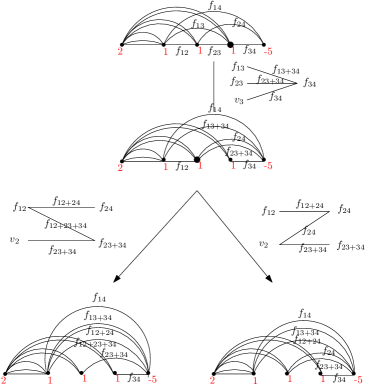
Figure 1. Reduction tree with root labeled by the graph $K_{4}(3,2,2):=([0,4],E(K_{4})\cup\{\{(0,1),(0,1),(0,1),(0,2),(0,2),(0,3),(0,3)\}\})$. The notation $f_{ij+jk}$ stands for the formal sum of edges $f_{ij}+f_{jk}$. The vertex of the graph where the reduction is taking place is enlarged. The flow polytopes corresponding to the leaves of the reduction tree dissect the flow polytope corresponding to the root of the tree, see Lemma 2.1.

Consider a graph $G$ on the vertex set $[n+1]$ with edges oriented from smaller to larger vertices and an integer netflow vector ${\bf a}=(a_{1},\ldots,a_{n},-\sum_{i}a_{i})$, with $a_{i}\geq 0$, $i\in[n]$. Pick an arbitrary vertex $i$,$1<i<n+1$, of $G$ as well as a submultiset $\mathcal{I}_{i}$ of the multiset of incoming edges to $i$ and submultiset $\mathcal{O}_{i}$ of the multiset of outgoing edges from $i$. Given an ordering on the sets $\mathcal{I}_{i}$ and $\mathcal{O}_{i}$ and a bipartite noncrossing tree $T\in\mathcal{T}_{\mathcal{I}_{i}\cup\{i\},\mathcal{O}_{i}}$, where $\mathcal{I}_{i}\cup\{i\}$ is ordered according to the order on $\mathcal{I}_{i}$ with $i$ appended as its last element,we describe the construction of new graphs $G^{(i)}_{T}(\mathcal{I}_{i},\mathcal{O}_{i})$ from $G$ as follows.

For each tree-edge $(e_{1},e_{2})$ of $T$ where $e_{1}=(r,i)\in\mathcal{I}_{i}$ and $e_{2}=(i,s)\in\mathcal{O}_{i}$ let $edge(e_{1},e_{2})=(r,s)$ and we let $edge(i,(i,j))=(i,j)$. We think of $edge(e_{1},e_{2})$ as a formal sum of the edges $e_{1}$ and $e_{2}$, where $edge(i,(i,j))=(i,j)$ as the edge $(i,j)$.

The graph $G^{(i)}_{T}(\mathcal{I}_{i},\mathcal{O}_{i})$ is then defined as the graph obtained from $G$ by deleting all edges in $\mathcal{I}_{i}\cup\mathcal{O}_{i}$ of $G$ and adding the multiset of edges $\{\{edge(e_{1},e_{2})~{}|~{}(e_{1},e_{2})\in E(T)\}\}\cup\{\{edge(i,(i,j))~{}|~{}(i,(i,j))\in E(T)\}\}.$ See Figure 1.

The difference in the above and that of [10, Section 3] is that in [10] the multisets $\mathcal{I}_{i}$ and $\mathcal{O}_{i}$ are always taken to equal to the multiset of incoming and the multiset of outgoing edges of $i$, whereas here we allow them to be proper submultisets of the multiset of incoming and the multiset of outgoing edges of $i$. Note that in the example on Figure 1 we have that $\mathcal{I}_{3}$ and $\mathcal{I}_{2}$ are proper subsets of the incoming edges at vertices 3, and 2, respectively.

The Subdivision Lemma, Lemma 2.1, states that $\mathcal{F}_{G}({\bf a})$ is a union over $T\in\mathcal{T}_{\mathcal{I}_{i}\cup\{i\},\mathcal{O}_{i}}$ of the smaller polytopes $\phi_{T}(\mathcal{F}_{G^{(i)}_{T}(\mathcal{I}_{i},\mathcal{O}_{i})}({\bf a})),$ where $\phi_{T}$ is an integral equivalence between $\mathcal{F}_{G^{(i)}_{T}(\mathcal{I}_{i},\mathcal{O}_{i})}({\bf a})$ and its image $\phi_{T}(\mathcal{F}_{G^{(i)}_{T}(\mathcal{I}_{i},\mathcal{O}_{i})}({\bf a}))$. We now define integrally equivalence of polytopes and the maps $\phi_{T}$.

Two polytopes $P_{1}\subseteq\mathbb{R}^{k_{1}}$ and ${P_{2}\subseteq\mathbb{R}^{k_{2}}}$ are integrally equivalent if there is an affine transformation $t:\mathbb{R}^{k_{1}}\to\mathbb{R}^{k_{2}}$ that is a bijection $P_{1}\to P_{2}$ and a bijection $\mathop{\mathrm{aff}}(P_{1})\cap\mathbb{Z}^{k_{1}}\to\mathop{\mathrm{aff}}(P_{2})\cap\mathbb{Z}^{k_{2}}$. Integrally equivalent polytopes have the same face lattice, volume, and Ehrhart polynomial.

Fix $T\in\mathcal{T}_{\mathcal{I}_{i}\cup\{i\},\mathcal{O}_{i}}$. Recall that $\mathcal{F}_{G^{(i)}_{T}(\mathcal{I}_{i},\mathcal{O}_{i})}({\bf a})\subset\mathbb{R}^{|E(G^{(i)}_{T}(\mathcal{I}_{i},\mathcal{O}_{i}))|}$ and denote the coordinates of $\mathbb{R}^{|E(G^{(i)}_{T}(\mathcal{I}_{i},\mathcal{O}_{i}))|}$ by $({\rm coord}_{e})_{e\in E(G^{(i)}_{T}(\mathcal{I}_{i},\mathcal{O}_{i}))}$; moreover, $\mathcal{F}_{G}({\bf a})\subset\mathbb{R}^{|E(G)|}$ and denote the coordinates of $\mathbb{R}^{|E(G)|}$ by $({\rm coord}_{d})_{d\in E(G)}$. Recall that each edge of $e\in G^{(i)}_{T}(\mathcal{I}_{i},\mathcal{O}_{i})$ is a sum of (one or more) edges of the original graph $G$; denote by $s(e)$ the subset of edges of $G$ which we sum in order to get $e$. Define the affine transformation $\phi_{T}:\mathbb{R}^{|E(G^{(i)}_{T}(\mathcal{I}_{i},\mathcal{O}_{i}))|}\to\mathbb{R}^{|E(G)|}$ via

$$\phi_{T}(({\rm c}_{e})_{e\in E(G^{(i)}_{T}(\mathcal{I}_{i},\mathcal{O}_{i}))})=({\rm c}_{d})_{d\in E(G)},\qquad\text{where}\qquad{\rm c}_{d}=\sum_{e:d\in s(e)}{\rm c}_{e}.$$

Note that $\phi_{T}$ is an invertible linear map between vector spaces of the same dimension which restricts to a bijection on the underlying lattice. Therefore $\phi_{T}$ is an integral equivalence between $\mathcal{F}_{G_{T}^{(i)}}(\mathcal{I}_{i},\mathcal{O}_{i})$ and its image in $\mathbb{R}^{|E(G)|}$. By definition, $\phi_{T}(\mathcal{F}_{G^{(i)}_{T}(\mathcal{I}_{i},\mathcal{O}_{i})}({\bf a}))\subseteq\mathcal{F}_{G}({\bf a})$. An illustration of the map $\phi_{T}$ appears on Figure 2.

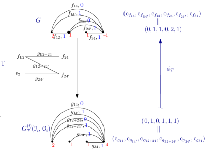
Figure 2. Illustration of $\phi_{T}(0,1,0,1,1,1)=(0,1,1,0,2,1)$. Note that we ordered the coordinates of $\mathbb{R}^{|E(G^{(i)}_{T}(\mathcal{I}_{i},\mathcal{O}_{i}))|}$ (where $i=2$, $\mathcal{I}_{i}=(f_{1,2})$ and $\mathcal{O}_{i})=(f_{24},f_{24^{\prime}})$) by ordering the edges of $G^{(i)}_{T}(\mathcal{I}_{i},\mathcal{O}_{i})$ in the order $({\rm c}_{g_{14}},{\rm c}_{g_{14^{\prime}}},{\rm c}_{g_{12+24}},{\rm c}_{g_{12+24^{\prime}}},{\rm c}_{g_{24^{\prime}}},{\rm c}_{g_{34}})$; we ordered the coordinates of $\mathbb{R}^{|E(G)|}$ by ordering the edges of $G$ in the order $({\rm c}_{f_{14}},{\rm c}_{f_{14^{\prime}}},{\rm c}_{f_{12}},{\rm c}_{f_{24}},{\rm c}_{f_{24^{\prime}}},{\rm c}_{f_{34}})$. We have that $s({g_{14}})=\{f_{14}\},s({g_{14^{\prime}}})=\{f_{14^{\prime}}\},s({g_{12+24}})=\{f_{12},f_{24}\},$ $s({g_{12+24^{\prime}}})=\{f_{12},f_{24^{\prime}}\},s({g_{24^{\prime}}})=\{f_{24^{\prime}}\},s({g_{34}})=\{f_{34}\}$.

By abuse of notation instead of writing $\phi_{T}(\mathcal{F}_{G^{(i)}_{T}(\mathcal{I}_{i},\mathcal{O}_{i})}({\bf a}))$ we write $\mathcal{F}_{G^{(i)}_{T}(\mathcal{I}_{i},\mathcal{O}_{i})}({\bf a})$ from now on, including in Lemma 2.1. With this convention we have $\mathcal{F}_{G^{(i)}_{T}(\mathcal{I}_{i},\mathcal{O}_{i})}({\bf a})\subseteq\mathcal{F}_{G}({\bf a})$.

The following Subdivision Lemma generalizes [10, Lemma 3.4]. The proof is analogous to that of [10, Lemma 3.4], and we leave it to the interested reader.

Lemma 2.1 (Subdivision Lemma).

Let $G$ be a graph on the vertex set $[n+1]$. Fix an integer netflow vector ${\bf a}=(a_{1},\ldots,a_{n},-\sum_{i=1}^{n}a_{i})$, $a_{i}\in\mathbb{Z}_{\geq 0}$ as well as a vertex $i\in\{2,\ldots,n\}$ and ordered multisets $\mathcal{I}_{i},\mathcal{O}_{i}$, which are submultisets of the multiset of incoming and outgoing edges incident to $i$. Then,

(2.1) $$\mathcal{F}_{G}({\bf a})=\bigcup_{T\in\mathcal{T}_{\mathcal{I}_{i}\cup\{i\},\mathcal{O}_{i}}}\mathcal{F}_{G^{(i)}_{T}(\mathcal{I}_{i},\mathcal{O}_{i})}({\bf a}).$$

Moreover, $\{\mathcal{F}_{G^{(i)}_{T}(\mathcal{I}_{i},\mathcal{O}_{i})}({\bf a})\}_{T\in\mathcal{T}_{\mathcal{I}_{i}\cup\{i\},\mathcal{O}_{i}}}$ are interior disjoint.

We refer to replacing $G$ by $\{G^{(i)}_{T}(\mathcal{I}_{i},\mathcal{O}_{i})\}_{T\in\mathcal{T}_{\mathcal{I}_{i}\cup\{i\},\mathcal{O}_{i}}}$ as in Lemma 2.1 as a reduction. We can encode a series of reductions on a flow polytope $\mathcal{F}_{G}({\bf a})$ in a rooted tree called a reduction tree with root $G$; see Figure 1 for an example. The root of this tree is the original graph $G$. After doing reductions on vertex $i$ with fixed $\mathcal{I}_{i},\mathcal{O}_{i}$ ordered submultisets of the multiset of incoming and outgoing edges incident to $i$, the descendant nodes of the root are the graphs ${G^{(i)}_{T}(\mathcal{I}_{i},\mathcal{O}_{i})}$, for $T\in\mathcal{T}_{\mathcal{I}_{i}\cup\{i\},\mathcal{O}_{i}}$. For each new node we decide whether to stop or repeat this process to define its descendants. The leaves of the reduction tree are those with no children. Note that the flow polytopes $\mathcal{F}_{H}({\bf a})$ of the graphs $H$ at the leaves of the reduction tree are interior disjoint and their union is $\mathcal{F}_{G}({\bf a})$ by repeated application of Lemma 2.1.

In [10] the authors used their less general version of Lemma 2.1 to define the canonical subdivision of flow polytopes $\mathcal{F}_{G}({\bf a})$. This allowed them in particular to derive (1.2) purely geometrically. We include their construction here and will use it in the next section.

Definition 2.2.

The canonical reduction tree $R_{G}$ for a graph $G$ on the vertex set $[n+1]$ is obtained by repeated use of Lemma 2.1 on the vertices $n,n-1,\ldots,2$ in this order and on the sets of edges $\mathcal{I}_{i}=\{\{(j,i)\in E(G)\mid j<i\}\}$ and $\mathcal{O}_{i}=\{\{(i,j)\in E(G)\mid i<j\}\}$, $i\in\{n,n-1,\ldots,2\},$ where both $\mathcal{I}_{i}$ and $\mathcal{O}_{i}$ are ordered by decreasing edge lengths.

For an example of a canonical reduction tree see Figure 3. Note that at each vertex $i$ the set $\mathcal{I}_{i}$ is all of the coming edges at $i$ (unlike in Figure 1) and the set $\mathcal{O}_{i}$ is the set of all outgoing edges at $i$.

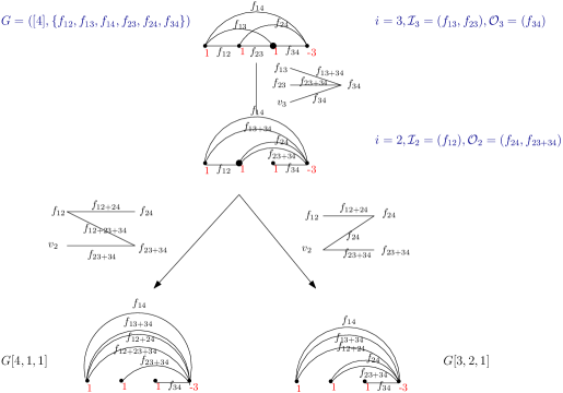
Figure 3. The canonical reduction tree for complete graph $K_{4}$ with nonnegative netflows on the first 3 vertices.

Definition 2.3.

Given a tuple ${\bf m}=(m_{1},\ldots,m_{n})$ of positive integers, let $G[{\bf m}]$ be the graph with vertices $[n+1]$ and $m_{i}$ edges $(i,n+1)$.

Note that the leaves of the canonical reduction tree in Figure 3 are both of the form $G[{\bf m}]$ for some ${\bf m}$; in particular the leaf on the left is $G[4,1,1]$ and the leaf on the right if $G[3,2,1]$. The following theorem states that this is no coincidence.

Recall that given graph $G$ on the vertex set $[n+1]$ we let ${\bf out}_{G}(i)=\it outdeg_{G}(i)-1$, where $\it outdeg_{G}(i)$ is the outdegree of vertex $i$ in $G$. We denote ${\bf out}_{G}=({\bf out}_{G}(1),\ldots,{\bf out}_{G}(n))$.

Theorem 2.4.

[10, Section 4] The canonical reduction tree $R_{G}$ of $G$ on the vertex set $[n+1]$ with $m$ edges has

$$\sum_{\begin{subarray}{c}{\bf j}\geq{\bf out}_{G}\\ j_{1}+\dots+j_{n}=m-n\end{subarray}}K_{G}(j_{1}-{\bf out}_{G}(1),\dots,j_{n}-{\bf out}_{G}(n),0)$$

leaves, where:

• the sum is over weak compositions ${\bf j}=(j_{1},j_{2},\ldots,j_{n})$ of $m-n$ that are $\geq({\rm out}(1),\ldots,{\rm out}(n))$ in dominance order, that is, $\sum_{k=1}^{l}j_{k}\geq\sum_{k=1}^{l}{\bf out}_{G}(k)$ for all $l\in[n]$;

• $K_{G}(j_{1}-{\bf out}_{G}(1),\dots,j_{n}-{\bf out}_{G}(n),0)$ of the leaves of $R_{G}$ are ${G[{\bf j+1}]}$;

• the polytopes $\mathcal{F}_{G[{\bf j+1}]}({\bf a})$ are interior disjoint and their union is $\mathcal{F}_{G}({\bf a})$;

• if $a_{i}>0$, $i\in[n]$, then the polytopes $\mathcal{F}_{G[{\bf j+1}]}({\bf a})$ are of the same dimension as $\mathcal{F}_{G}({\bf a})$.

The polytopes specified in Theorem 2.4 are the top dimensional polytopes in the canonical subdivision of $\mathcal{F}_{G}({\bf a})$ [10].

Example 2.5.

Let us apply Theorem 2.4 to the canonical reduction tree $R_{K_{4}}$ from Figure 3. Here $n=3$ and $m=6$. We have that $(\it outdeg_{K_{4}}(1),\it outdeg_{K_{4}}(2),\it outdeg_{K_{4}}(3))=(3,2,1)$ and thus, $({\bf out}_{K_{4}}(1),{\bf out}_{K_{4}}(2),{\bf out}_{K_{4}}(3))=(2,1,0)$. The sum in Theorem 2.4 is over compositions ${\bf j}=(j_{1},j_{2},j_{3})$ of $3$ that are $\geq(2,1,0)$ in dominance order. Thus, the two possible ${\bf j}$’s are $(3,0,0)$ and $(2,1,0)$. The first two points of Theorem 2.4 thus state that there are $K_{K_{4}}(3-2,0-1,0-0,0)=1$ leaves of $R_{K_{4}}$ that are ${G[4,1,1]}$ and $K_{K_{4}}(2-2,1-1,0-0,0)=1$ leaves of $R_{K_{4}}$ that are ${G[3,2,1]}$; see Figure 3.

3. A few geometric insights

This section collects the main insights necessary for proving (1.3) purely geometrically. The proof of (1.3) relies on stringing all the following statements together in order to give a proof of it in Theorem 4.1. As mentioned in the previous section: we reinterpret the left hand side of (1.3) as a volume of a flow polytope (namely, of $\mathcal{F}_{{G({\bf c})}}(e_{1}-e_{n+2})$, see Definition 3.1 for the meaning of ${G({\bf c})}$), and then the right hand side can be obtained by summing volumes of polytopes in a subdivision of our new flow polytope.

Definition 3.1.

Fix a vector ${\bf c}=(c_{1},\dots,c_{n})\in\mathbb{Z}^{n}_{>0}$ and a graph $G$ on the vertex set $[n+1]$. The graph ${G({\bf c})}$ is defined to be the graph obtained by adding a source vertex $0$ to $V(G)$, so that $V({G({\bf c})})=[0,n+1]$, along with $c_{i}$ edges edges $(0,i)$, for every $i\in[n]$, to $E(G)$. Formally, we have

$$G({\bf c}):=(V(G)\cup\{0\},E(G)\cup\{\{(0,i)^{c_{i}}\mid i\in[n]\}\}),$$

where $(0,i)^{c_{i}}$ signifies $c_{i}$ copies of the edge $(0,i)$. Note that the graph ${G({\bf c})}$ restricted to the vertex set $[n+1]$ is equal to the graph $G$.

Of importance in Definition 3.1 is that when we restrict ${G({\bf c})}$ to the vertex set $[n+1],$ we get $G$ back. This allows us to use our full knowledge of canonical reduction trees, as given in Theorem 2.4. This is because Lemma 2.1 allows for not using all the incoming (or outgoing) edges at a vertex – and yet if we use all incoming and outgoing edges that are in a given subgraph of the graph, we can still invoke Theorem 2.4 for the mentioned subgraph! Details are spelled out in Theorem 3.5 below.

Recall that given graph $G$ on the vertex set $[n+1]$ we let ${\bf in}_{G}(i)=\it indeg_{G}(i)-1$, where $\it indeg_{G}(i)$ is the indegree of vertex $i$ in $G$.

With Definition 3.1 we have that:

Lemma 3.2.

Fix a vector ${\bf c}=(c_{1},\dots,c_{n})\in\mathbb{Z}^{n}_{>0}$ and a graph $G$ on the vertex set $[n+1]$. Define $a_{i}\colonequals{\bf in}_{G}(i)+c_{i}$. The number of integer points in $\mathcal{F}_{G}(a_{1},\dots,a_{n},-\sum_{i=1}^{n}a_{i})$ is equal to the number of integer points in the flow polytope $\mathcal{F}_{G({\bf c})}(0,{\bf in}_{{G({\bf c})}}(1),\dots,{\bf in}_{{G({\bf c})}}(n),-\sum_{i=1}^{n}{\bf in}_{{G({\bf c})}}(i))$. In other words,

$$K_{G}\bigg{(}a_{1},\dots,a_{n},-\sum_{i=1}^{n}a_{i}\bigg{)}=K_{{G({\bf c})}}\bigg{(}0,{\bf in}_{{G({\bf c})}}(1),\dots,{\bf in}_{{G({\bf c})}}(n),-\sum_{i=1}^{n}{\bf in}_{{G({\bf c})}}(i)\bigg{)}.$$

Proof.

Consider an integer $(0,{\bf in}_{{G({\bf c})}}(1),\dots,{\bf in}_{{G({\bf c})}}(n),-\sum_{i=1}^{n}{\bf in}_{{G({\bf c})}}(i))$-flow $f$ on the graph $G({\bf c})$. Note that when we restrict $f$ to $G\subset{G({\bf c})}$ it is an $({\bf in}_{{G({\bf c})}}(1),\dots,{\bf in}_{{G({\bf c})}}(n),-\sum_{i=1}^{n}{\bf in}_{{G({\bf c})}}(i))$-flow on $G$. By the definition of ${G({\bf c})}$, we have ${\bf in}_{{G({\bf c})}}(i)={\bf in}_{G}(i)+c_{i}=a_{i}$. Thus, an integer $(0,{\bf in}_{{G({\bf c})}}(1),\dots,{\bf in}_{{G({\bf c})}}(n),-\sum_{i=1}^{n}{\bf in}_{{G({\bf c})}}(i))$-flow on ${G({\bf c})}$ restricts to an integer $(a_{1},\dots,a_{n},$ $-\sum_{i=1}^{n}a_{i})$-flow on $G$. This is clearly a bijection showing that the number of integer $(0,{\bf in}_{{G({\bf c})}}(1),\dots,$ ${\bf in}_{{G({\bf c})}}(n),-\sum_{i=1}^{n}{\bf in}_{{G({\bf c})}}(i))$-flows on ${G({\bf c})}$ equals to the number of integer $(a_{1},\dots,a_{n},-\sum_{i=1}^{n}a_{i})$-flows on $G$. The latter equal $K_{{G({\bf c})}}(0,{\bf in}_{{G({\bf c})}}(1),\dots,{\bf in}_{{G({\bf c})}}(n),-\sum_{i=1}^{n}{\bf in}_{{G({\bf c})}}(i))$ and $K_{G}(a_{1},\dots,a_{n},-\sum_{i=1}^{n}a_{i})$, respectively. ∎

3.3. Dissecting $\mathcal{F}_{{G({\bf c})}}(e_{1}-e_{n+2})$.

In this section we show how to dissect $\mathcal{F}_{{G({\bf c})}}(e_{1}-e_{n+2})$, ${\bf c}\in\mathbb{Z}^{n}_{>0}$, into

$$\sum_{\begin{subarray}{c}{\bf j}\geq{\bf out}_{G}\\ j_{1}+\dots+j_{n}=m-n\end{subarray}}\frac{(c_{1})_{j_{1}}}{j_{1}!}\dots\frac{(c_{n})_{j_{n}}}{j_{n}!}K_{G}(j_{1}-{\bf out}_{G}(1),\dots,j_{n}-{\bf out}_{G}(n),0)$$

many unimodular simplices. The notation $(k)_{j}$ stands for $(k)_{j}:=k(k-1)\cdots(k-j+1)$.

Definition 3.4.

Given a graph $G$ on the vertex set $[n+1]$ define the reduction tree $R_{G}^{\bf c}$ with root ${G({\bf c})}$ as the reduction tree obtained by repeated use of Lemma 2.1 on the vertices $n,n-1,\ldots,2$ in this order and on the sets of edges $\mathcal{I}_{i}=\{\{(j,i)\in E(G)\mid j<i\}\}$ and $\mathcal{O}_{i}=\{\{(i,j)\in E(G)\mid i<j\}\}$, $i\in\{n,n-1,\ldots,2\},$ where both $\mathcal{I}_{i}$ and $\mathcal{O}_{i}$ are ordered by decreasing edge lengths.

We note that Definition 3.4 is set up so that if we delete all edges incident to $0$ in the graphs labeling the nodes of $R_{G}^{\bf c}$ we obtain the canonical reduction tree $R_{G}$ of $G$ as in Definition 2.2. For an example of the reduction tree $R_{K_{4}}^{(3,2,2)}$ see Figure 1; compare this with the canonical reduction tree $R_{K_{4}}$ on Figure 3.

Theorem 3.5.

Fix ${\bf c}\in\mathbb{Z}^{n}_{>0}$. Given a graph $G$ on the vertex set $[n+1]$ with $m$ edges, the reduction tree $R_{G}^{\bf c}$ of ${G({\bf c})}$ has

$$\sum_{\begin{subarray}{c}{\bf j}\geq{\bf out}_{G}\\ j_{1}+\dots+j_{n}=m-n\end{subarray}}K_{G}(j_{1}-{\bf out}_{G}(1),\dots,j_{n}-{\bf out}_{G}(n),0)$$

leaves, where:

• the sum is over weak compositions ${\bf j}=(j_{1},j_{2},\ldots,j_{n})$ of $m-n$ that are $\geq({\rm out}_{1},\ldots,{\rm out}_{n})$ in dominance order;

• $K_{G}(j_{1}-{\bf out}_{G}(1),\dots,j_{n}-{\bf out}_{G}(n),0)$ of the leaves of $R_{G}^{\bf c}$ are ${G[{\bf j+1}]({\bf c})}$;

• the polytopes $\mathcal{F}_{G[{\bf j+1}]({\bf c})}({e_{1}-e_{n+2}})$ are interior disjoint and their union is $\mathcal{F}_{{G({\bf c})}}(e_{1}-e_{n+2})$;

• the polytopes $\mathcal{F}_{G[{\bf j+1}]({\bf c})}({e_{1}-e_{n+2}})$ are of the same dimension as $\mathcal{F}_{{G({\bf c})}}(e_{1}-e_{n+2})$.

Before proceeding with the proof of Theorem 3.5, we illustrate it with an example. Compare this to Example 2.5.

Example 3.6.

Let us apply Theorem 3.5 to the reduction tree $R_{K_{4}}^{(3,2,2)}$ from Figure 1. Here $n=3$ and $m=6$. We have that $(\it outdeg_{K_{4}}(1),\it outdeg_{K_{4}}(2),\it outdeg_{K_{4}}(3))=(3,2,1)$ and thus, $({\bf out}_{K_{4}}(1),{\bf out}_{K_{4}}(2),{\bf out}_{K_{4}}(3))=(2,1,0)$. The sum in Theorem 3.5 is over compositions ${\bf j}=(j_{1},j_{2},j_{3})$ of $3$ that are $\geq(2,1,0)$ in dominance order. Thus, the two possible ${\bf j}$’s are $(3,0,0)$ and $(2,1,0)$. The first two points of Theorem 3.5 thus state that there are $K_{K_{4}}(3-2,0-1,0-0,0)=1$ leaves of $R_{K_{4}}^{(3,2,2)}$ that are ${G[4,1,1]}(3,2,2)$ and $K_{K_{4}}(2-2,1-1,0-0,0)=1$ leaves of $R_{K_{4}}^{(3,2,2)}$ that are ${G[3,2,1]}(3,2,2)$; see Figure 1.

Proof of Theorem 3.5 Definitions 2.2 and 3.4 are set up so that appealing to Lemma 2.1 and Theorem 2.4 instantly implies the first three statements of Theorem 3.5. It remains to show that the polytopes $\mathcal{F}_{G[{\bf j+1}]({\bf c})}({e_{1}-e_{n+2}})$ are of the same dimension as $\mathcal{F}_{{G({\bf c})}}(e_{1}-e_{n+2})$. Since the dimension of $\mathcal{F}_{H}(e_{1}-e_{n+2})$, where $H$ is a graph on the vertex set $[0,n+1]$ is $|E(H)|-|V(H)|+1$, the same dimensionality of $\mathcal{F}_{G[{\bf j+1}]({\bf c})}({e_{1}-e_{n+2}})$ and $\mathcal{F}_{{G({\bf c})}}(e_{1}-e_{n+2})$ readily follows for ${\bf j}\geq{\bf out}_{G},j_{1}+\dots+j_{n}=m-n.$ ∎

Lemma 3.7.

Fix ${\bf c}\in\mathbb{Z}^{n}_{>0}$. There is a dissection of $\mathcal{F}_{G[{\bf j+1}]({\bf c})}(e_{1}-e_{n+2})$ into $\frac{(c_{1})_{j_{1}}}{j_{1}!}\dots\frac{(c_{n})_{j_{n}}}{j_{n}!}$ many unimodular simplices.

Before giving a proof of Lemma 3.7 we include a version of the Subdivision Lemma appearing in [10, Lemma 3.4].

Lemma 3.8.

[10, Lemma 3.4] Let $\{\mathcal{F}_{G^{(i)}_{T}(\mathcal{I}_{i},\mathcal{O}_{i})}({\bf a})\}_{T\in\mathcal{T}_{\mathcal{I}_{i}\cup\{i\},\mathcal{O}_{i}}}$ as in Lemma 2.1. Let $\mathcal{I}_{i},\mathcal{O}_{i}$ be the multiset of incoming and outgoing edges incident to $i$, with fixed arbitrary ordering. Assume that $a_{i}=0$. Then, it is exactly those of the polytopes among $\{\mathcal{F}_{G^{(i)}_{T}(\mathcal{I}_{i},\mathcal{O}_{i})}({\bf a})\}_{T\in\mathcal{T}_{\mathcal{I}_{i}\cup\{i\},\mathcal{O}_{i}}}$ that are of the same dimension as $\mathcal{F}_{G}({\bf a})$ for which there is exactly one edge incident to $i$ in $T\in\mathcal{T}_{\mathcal{I}_{i}\cup\{i\},\mathcal{O}_{i}}$. Such polytopes form a dissection of $\mathcal{F}_{G}({\bf a})$.

Proof of Lemma 3.7. Repeatedly use Lemma 3.8 for the case of netflow vector coordinate value $0$ on the vertices $1,2,\ldots,n$ of $G[{\bf j+1}]({\bf c})$. This amounts to picking tuples of bipartite noncrossing trees $(T_{1},\ldots,T_{n})\in\mathcal{T}_{L_{1},R_{1}}\times\cdots\times\mathcal{T}_{L_{n},R_{n}}$, where $|L_{i}|=c_{i}$ and $|R_{i}|=j_{i}+1$, for $i\in[n]$. The number of such tuples is $\frac{(c_{1})_{j_{1}}}{j_{1}!}\dots\frac{(c_{n})_{j_{n}}}{j_{n}!},$ since $\frac{(c_{i})_{j_{i}}}{j_{i}!}=\#\mathcal{T}_{L_{i},R_{i}}$.∎

Theorem 3.9.

Fix ${\bf c}\in\mathbb{Z}^{n}_{>0}$. There is a dissection of $\mathcal{F}_{{G({\bf c})}}(e_{1}-e_{n+2})$ into

$$\sum_{\begin{subarray}{c}{\bf j}\geq{\bf out}_{G}\\ j_{1}+\dots+j_{n}=m-n\end{subarray}}\frac{(c_{1})_{j_{1}}}{j_{1}!}\dots\frac{(c_{n})_{j_{n}}}{j_{n}!}K_{G}(j_{1}-{\bf out}_{G}(1),\dots,j_{n}-{\bf out}_{G}(n),0)$$

many unimodular simplices.

Proof.

Follows readily from Theorem 3.5 and Lemma 3.7.∎

4. The geometric proof of (1.3)

In this section we prove the Baldoni–Vergne–Lidskii integer point formula (1.3) from Theorem 1.1. As mentioned in the Introduction, the original proof by Baldoni and Vergne [1] relies on residue calculations and a second, combinatorial proof by Mészáros and Morales [10] makes use of a canonical subdivision of flow polytopes and generating functions of Kostant partition functions to prove (1.3). In contrast, here we give a purely geometric proof of (1.3). For the reader’s reference we rewrite (1.3) in Theorem 4.1 in the form that we prove it:

Theorem 4.1.

Let $G$ be a connected graph on vertex set $[n+1]$ so that $G$ has at least one outgoing edge at vertex $i$ for $i\leq n$. For $i\in[n]$ we set ${\bf in}_{G}(i)\colonequals\it indeg_{G}(i)-1$ and ${\bf out}_{G}(i)\colonequals\it outdeg_{G}(i)-1$. Fix positive integers $c_{1},\dots,c_{n}$. Let $a_{i}\colonequals{\bf in}_{G}(i)+c_{i}$. Then we have

$$K_{G}\bigg{(}a_{1},\dots,a_{n},-\sum_{i=1}^{n}a_{i}\bigg{)}=\sum_{\begin{subarray}{c}{\bf j}\geq{\bf out}_{G}\\ j_{1}+\dots+j_{n}=m-n\end{subarray}}\frac{(c_{1})_{j_{1}}}{j_{1}!}\dots\frac{(c_{n})_{j_{n}}}{j_{n}!}K_{G}(j_{1}-{\bf out}_{G}(1),\dots,j_{n}-{\bf out}_{G}(n),0),$$

where $\geq$ denotes the dominance order, that is, $j_{1}+\dots+j_{k}\geq{\bf out}_{G}(1)+\dots+({\bf out}_{G})_{k}$ for all $k\in[n]$, and $(n)_{k}\colonequals n(n+1)\dots(n+k-1)$.

Proof.

Given a vector ${\bf c}:=(c_{1},\dots,c_{n})\in\mathbb{Z}^{n}_{>0}$ and a graph $G$ on the vertex set $[n+1]$, we defined $G(\bf c)$ on the vertex set $[0,n+1]$ so that

$$K_{G}\bigg{(}a_{1},\dots,a_{n},-\sum_{i=1}^{n}a_{i}\bigg{)}=K_{{G({\bf c})}}\bigg{(}0,{\bf in}_{{G({\bf c})}}(1),\dots,{\bf in}_{{G({\bf c})}}(n),-\sum_{i=1}^{n}{\bf in}_{{G({\bf c})}}(i)\bigg{)},$$

where $a_{i}\colonequals{\bf in}_{G}(i)+c_{i}$. See Definition 3.1 and Lemma 3.2.

By (1.2) the normalized volume of $\mathcal{F}_{{G({\bf c})}}(e_{1}-e_{n+2})$ is precisely

$$K_{{G({\bf c})}}(0,{\bf in}_{{G({\bf c})}}(1),\dots,{\bf in}_{{G({\bf c})}}(n),-\sum_{i=1}^{n}{\bf in}_{{G({\bf c})}}(i)).$$

(Recall that the proof of (1.2) given in [10] via the canonical subdivision is fully geometric.) In particular, the number of simplices in a unimodular triangulation of $\mathcal{F}_{{G({\bf c})}}(e_{1}-e_{n+2})$ is

$$K_{{G({\bf c})}}(0,{\bf in}_{{G({\bf c})}}(1),\dots,{\bf in}_{{G({\bf c})}}(n),-\sum_{i=1}^{n}{\bf in}_{{G({\bf c})}}(i)).$$

By Theorem 3.9 there is a dissection of $\mathcal{F}_{{G({\bf c})}}(e_{1}-e_{n+2})$ into

$$\sum_{\begin{subarray}{c}{\bf j}\geq{\bf out}_{G}\\ j_{1}+\dots+j_{n}=m-n\end{subarray}}\frac{(c_{1})_{j_{1}}}{j_{1}!}\dots\frac{(c_{n})_{j_{n}}}{j_{n}!}K_{G}(j_{1}-{\bf out}_{G}(1),\dots,j_{n}-{\bf out}_{G}(n),0)$$

many unimodular simplices.

Thus, chaining all the equalities we get that

$$K_{G}\bigg{(}a_{1},\dots,a_{n},-\sum_{i=1}^{n}a_{i}\bigg{)} =K_{{G({\bf c})}}\bigg{(}0,{\bf in}_{{G({\bf c})}}(1),\dots,{\bf in}_{{G({\bf c})}}(n),-\sum_{i=1}^{n}{\bf in}_{{G({\bf c})}}(i)\bigg{)}$$

$$=\sum_{\begin{subarray}{c}{\bf j}\geq{\bf out}_{G}\\ j_{1}+\dots+j_{n}=m-n\end{subarray}}\frac{(c_{1})_{j_{1}}}{j_{1}!}\dots\frac{(c_{n})_{j_{n}}}{j_{n}!}K_{G}(j_{1}-{\bf out}_{G}(1),\dots,j_{n}-{\bf out}_{G}(n),0),$$

to obtain Theorem  4.1. ∎

5. Concluding remarks

Faced with the formulas for volume and integer point count of flow polytopes given in equations (1.2) and (1.3), one instantly observes the nonnegativity of the quantities involved. Yet, the original proof of Baldoni and Vergne [1] is via residue calculations: involving complex numbers and subtractions.

When we study manifestly nonnegative quantities, as in equations (1.2) and (1.3), it is natural to seek a manifestly nonnegative proof: a proof devoid of subtraction (and complex numbers). A geometric proof can make this aspiration a reality. A geometric construction was used by Mészáros and Morales [10] to prove (1.2) in a manifestly nonnegative way and the present paper accomplishes the same goal via geometric constructions for (1.3).

References

- [1] W. Baldoni and M. Vergne. Kostant partitions functions and flow polytopes. Transform. Groups, 13(3-4):447–469, 2008.
- [2] W. Baldoni-Silva, J. A. De Loera, and M. Vergne. Counting integer flows in networks. Found. Comput. Math., 4(3):277–314, 2004.
- [3] J. A. De Loera and B. Sturmfels. Algebraic unimodular counting. Math. Program., 96(2, Ser. B):183–203, 2003. Algebraic and geometric methods in discrete optimization.
- [4] S. C.. Gutekunst, K. Mészáros, and T. K. Petersen. Root cones and the resonance arrangement. ArXiv e-prints, 2019.
- [5] A. N. Kirillov. Ubiquity of Kostka polynomials. In Physics and combinatorics 1999 (Nagoya), pages 85–200. World Sci. Publ., River Edge, NJ, 2001.
- [6] B. Kostant. A formula for the multiplicity of a weight. Proc. Nat. Acad. Sci. U.S.A., 44:588–589, 1958.
- [7] B. Kostant. A formula for the multiplicity of a weight. Trans. Amer. Math. Soc., 93:53–73, 1959.
- [8] R. I. Liu, K. Mészáros, and A. H. Morales. Flow polytopes and the space of diagonal harmonics. Canadian Journal of Mathematics, 71(6):1495–1521, 2019.
- [9] K. Mészáros and A. H. Morales. Flow polytopes of signed graphs and the Kostant partition function. Int. Math. Res. Not. IMRN, (3):830–871, 2015.
- [10] K. Mészáros and A. H. Morales. Volumes and Ehrhart polynomials of flow polytopes. Math. Z.,, (293):1369–1401, 2019.
- [11] K. Mészáros, A. H. Morales, and B. Rhoades. The polytope of Tesler matrices. Selecta Math. (N.S.), 23(1):425–454, 2017.
- [12] K. Mészáros and A. St. Dizier. From generalized permutahedra to grothendieck polynomials via flow polytopes. Algebraic Combinatorics, 3(5):1197–1229, 2020.
- [13] A Schrijver. Combinatorial optimization. Polyhedra and efficiency. Vol. B, volume 24 of Algorithms and Combinatorics. Springer-Verlag, Berlin, 2003. Matroids, trees, stable sets, Chapters 39–69.
- [14] B. Sturmfels. On vector partition functions. J. Combin. Theory Ser. A, 72(2):302–309, 1995.