1

Associated Learning: Decomposing End-to-end Backpropagation Based on Autoencoders and Target Propagation

Yu-Wei Kao, Hung-Hsuan Chen
Department of Computer Science and Information Engineering, National Central University

Keywords: Backpropagation, pipelined training, parallel training, backward locking, associated learning

Abstract

Backpropagation (BP) is the cornerstone of today’s deep learning algorithms, but it is inefficient partially because of backward locking, which means updating the weights of one layer locks the weight updates in the other layers. Consequently, it is challenging to apply parallel computing or a pipeline structure to update the weights in different layers simultaneously. In this paper, we introduce a novel learning structure called associated learning (AL), which modularizes the network into smaller components, each of which has a local objective. Because the objectives are mutually independent, AL can learn the parameters in different layers independently and simultaneously, so it is feasible to apply a pipeline structure to improve the training throughput. Specifically, this pipeline structure improves the complexity of the training time from $O(n\ell)$, which is the time complexity when using BP and stochastic gradient descent (SGD) for training, to $O(n+\ell)$, where $n$ is the number of training instances and $\ell$ is the number of hidden layers. Surprisingly, even though most of the parameters in AL do not directly interact with the target variable, training deep models by this method yields accuracies comparable to those from models trained using typical BP methods, in which all parameters are used to predict the target variable. Consequently, because of the scalability and the predictive power demonstrated in the experiments, AL deserves further study to determine the better hyperparameter settings, such as activation function selection, learning rate scheduling, and weight initialization, to accumulate experience, as we have done over the years with the typical BP method. Additionally, perhaps our design can also inspire new network designs for deep learning. Our implementation is available at https://github.com/SamYWK/Associated_Learning.

1 Introduction

Deep neural networks are usually trained using backpropagation (BP) (Rumelhart et al., 1986), which, although common, increases the training difficulty for several reasons, among which backward locking highly limits the training speed. Essentially, the end-to-end training method propagates the error-correcting signals layer by layer; consequently, it cannot update the network parameters of the different layers in parallel. This backward locking problem is discussed in (Jaderberg et al., 2016). Backward locking becomes a severe performance bottleneck when the network has many layers. Beyond these computational weaknesses, BP-based learning seems biologically implausible. For example, it is unlikely that all the weights would be adjusted sequentially and in small increments based on a single objective (Crick, 1989). Additionally, some components essential for BP to work correctly have not been observed in the cortex (Balduzzi et al., 2015). Therefore, many works have proposed methods that more closely resemble the operations of biological neurons (Lillicrap et al., 2016; Nøkland, 2016; Bartunov et al., 2018; Nøkland and Eidnes, 2019). However, empirical studies show that the predictions of these methods are still unsatisfactory compared to those using BP (Bartunov et al., 2018).

In this paper, we propose associated learning (AL), a method that can be used to replace end-to-end BP when training a deep neural network. AL decomposes the network into small components such that each component has a local objective function independent of the local objective functions of the other components. Consequently, the parameters in different components can be updated simultaneously, meaning that we can leverage parallel computing or pipelining to improve the training throughput. We conducted experiments on different datasets to show that AL gives test accuracies comparable to those obtained by end-to-end BP training, even though most components in AL do not directly receive the residual signal from the output layer.

The remainder of this paper is organized as follows. In Section 2, we review the related works regarding the computational issues of training deep neural networks. Section 3 gives a toy example to compare end-to-end BP with our proposed AL method. Section 4 explains the details of AL. We conducted extensive experiments to compare AL and BP-based end-to-end learning using different types of neural networks and different datasets, and the results are shown in Section 5. Finally, we discuss the discoveries and suggest future work in Section 6.

2 Related Work

BP (Rumelhart et al., 1986) is an essential algorithm for training deep neural networks and is the foundation of the success of many models in recent decades (Hochreiter and Schmidhuber, 1997; LeCun et al., 1998; He et al., 2016). However, because of “backward locking” (i.e., the weights must be updated layer by layer), training a deep neural network can be extremely inefficient (Jaderberg et al., 2016). Additionally, empirical evidence shows that BP is biologically implausible (Crick, 1989; Balduzzi et al., 2015; Bengio et al., 2015). Thus, many studies have suggested replacing BP with a more biologically plausible method or with a gradient-free method (Taylor et al., 2016; Ororbia and Mali, 2019; Ororbia et al., 2018) in the hope of decreasing the computational time and memory consumption and better resembling biological neural networks (Bengio et al., 2015; Huo et al., 2018a, b).

To address the backward locking problem, the authors of (Jaderberg et al., 2016) proposed using a synthetic gradient, which is an estimation of the real gradient generated by a separate neural network for each layer. By adopting the synthetic gradient as the actual gradient, the parameters of every layer can be updated simultaneously and independently. This approach eliminates the backward locking problem. However, the experimental results have shown that this approach tends to result in underfitting—probably because the gradients are difficult to predict.

It is also possible to eliminate backward locking by computing the local errors for the different components of a network. In (Belilovsky et al., 2018), the authors showed that using an auxiliary classifier for each layer can yield good results. However, this paper added one layer to the network at a time, so it was challenging for the network to learn the parameters of different layers in parallel. In (Mostafa et al., 2018), every layer in a deep neural network is trained by a local classifier. However, experimental results have shown that this type of model is not comparable with BP. The authors of (Belilovsky et al., 2019) and the authors of (Nøkland and Eidnes, 2019) also proposed to update parameters based on (or partially based on) local errors. These models indeed allow the simultaneous updating of parameters of different layers, and experimental results showed that these techniques improved testing accuracy. However, these designs require each local component to receive signals directly from the target variable for loss computation. Biologically, it is unlikely that neurons far away from the target would be able to access the target signal directly. Therefore, even though these methods do not require global BP, they may still be biologically implausible.

Feedback alignment (Lillicrap et al., 2016) suggests propagating error signals in a similar manner as BP, but the error signals are propagated with fixed random weights in every layer. Later, the authors of (Nøkland, 2016) suggested delivering error signals directly from the output layer using fixed weights. The result is that the gradients are propagated by weights, while the signals remain local to each layer. The problem with this approach is that it is similar to the issue discussed in the preceding paragraph—biologically, distant neurons are unlikely to be able to obtain signals directly from the target variable.

Another biologically motivated algorithm is target propagation (Bengio, 2014; Lee et al., 2015; Bartunov et al., 2018). Rather than computing the gradient for every layer, the target propagation computes the target that each layer should learn. This approach relies on an autoencoder (Baldi, 2012) to calculate the inverse mapping of the forward pass and then pass the ground truth information to every layer. Each training step includes two losses that must be minimized for each layer: the loss of inverse mapping and the loss between activations and targets. This learning method alleviates the need for symmetric weights and is both biologically plausible and more robust than BP when applied to stochastic networks. Nonetheless, the targets are still generated layer by layer.

Overviews of the biologically plausible (or at least partially plausible) methods are presented in (Bengio et al., 2015; Bartunov et al., 2018). Although most of these methods perform worse than conventional BP, optimization beyond BP is still an important research area, mainly for computational efficiency and biological compatibility reasons.

Most studies on parallelizing deep learning distribute different data instances into different computing units. Each of these computing units computes the gradient based on the allocated instances, and the final gradient is determined by an aggregation of the gradients computed by all the computing units (Shallue et al., 2018; Zinkevich et al., 2010). Although this indeed increases the training throughput via parallelization, this is different from our approach because our method parallelizes the computation in different layers of a deep network. Our AL technique and the technique of parallelizing data instances can complement each other and further improve the throughput given enough computational resources. A recent work, GPipe, utilizes pipeline training to improve the training throughput (Huang et al., 2019). However, all the parameters in GPipe are still influenced in a layerwise fashion. Our method is different because the parameters in the different layers are independent.

Our work is highly motivated by target propagation, but we create intermediate mappings instead of directly transforming features into targets. As a result, the local signals in each layer are independent of the signals in the other layers, and most of these signals are not obtained directly from the output label.

3 A Toy Example to Compare the Training Throughput of End-to-end Backpropagation and Associated Learning

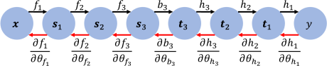
Figure 1: An example of a deep neural network with 6 hidden layers. We denote each forward function ($f_{1},f_{2},f_{3},b_{3},h_{3},h_{2},h_{1}$) and the output of each function ($s_{1},s_{2},s_{3},t_{3},t_{2},t_{1},y$) by different symbols for ease of later explanation. Let $\theta^{(f)}$ denote the parameters of a function $f$; then, the backward path requires computing the local gradient $\frac{\partial f}{\partial\theta^{(f)}}$ for each function $f$.

Figure 1 gives a typical structure of a deep neural network with 6 hidden layers. The input feature vector $\boldsymbol{x}$ goes through a series of transformations ($\boldsymbol{x}\xrightarrow{f_{1}}\boldsymbol{s}_{1}\xrightarrow{f_{2}}\boldsymbol{s}_{2}\xrightarrow{f_{3}}\boldsymbol{s}_{3}\xrightarrow{b_{3}}\boldsymbol{t}_{3}\xrightarrow{h_{3}}\boldsymbol{t}_{2}\xrightarrow{h_{2}}\boldsymbol{t}_{1}\xrightarrow{h_{1}}y$) to approximate the corresponding output $y$. We denote the functions ($f_{1},f_{2},f_{3},b_{3},t_{3},t_{2},t_{1}$) and the outputs of these functions ($s_{1},s_{2},s_{3},t_{3},t_{2},t_{1},y$) by different symbols for the ease of later explanation on AL. If stochastic gradient descent (SGD) and BP are applied to search for the proper parameter values, we need to compute the local gradient $\frac{\partial f}{\partial\theta^{(f)}}$ as the backward function for every forward function $f$ (whose parameters are denoted by $\theta^{(f)}$). As a result, each training epoch requires a time complexity of $O(n\times((\ell+1)+(\ell+1)))\approx O(n\ell)$, in which $n$ is the number of training instances and $\ell$ is the number of hidden layers (i.e., $\ell=6$ in our example). Since both forward pass and backward pass require $\ell+1$ transformations, we have two $\ell+1$ terms. Consequently, the training time increases linearly with the number of hidden layers $\ell$.

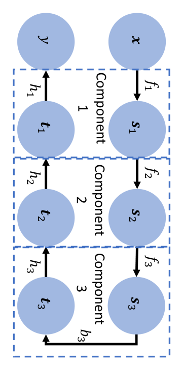
Figure 2: A simplified structure of the AL technique, which decomposes 6 hidden layers into 3 components such that each component has a local objective function that is independent of the objective functions of the other components. Consequently, we may update the parameters in component $i$ $(\theta^{(f)}_{i},\theta^{(h)}_{i})$ and the parameters in component $j$ $(\theta^{(f)}_{j},\theta^{(h)}_{j})$ simultaneously for $i\neq j$.

Table 1: An example of simultaneously updating the parameters by pipelining

Time unit	1	2	3	4	5	6	7	…
$1^{\textrm{st}}$ mini-batch	Task 1	Task 2	Task 3
$2^{\textrm{nd}}$ mini-batch		Task 1	Task 2	Task 3
$3^{\textrm{rd}}$ mini-batch			Task 1	Task 2	Task 3
$4^{\textrm{th}}$ mini-batch				Task 1	Task 2	Task 3
$5^{\textrm{th}}$ mini-batch					Task 1	Task 2	Task 3
…

Figure 2 shows a simplified structure of the AL technique, which “folds” the network and decomposes the network into 3 components such that each component has a local objective function that is independent of the local objectives in the other components. As a result, for $i\neq j$, we may update the parameters in component $i$ $(\theta^{(f)}_{i},\theta^{(h)}_{i})$ and the parameters in component $j$ $(\theta^{(f)}_{j},\theta^{(h)}_{j})$ independently and simultaneously, since the parameters of component $i$ ($(\theta^{(f)}_{i},\theta^{(h)}_{i})$) determine the loss of component $i$, which is independent of the loss of component $j$, which is determined by the parameters of component $j$ ($(\theta^{(f)}_{j},\theta^{(h)}_{j})$).

Table 1 gives an example of applying pipelining for parameter updating to improve the training throughput using AL. Let Task $i$ be the task of updating the parameters in Component $i$. At the $1^{\textrm{st}}$ time unit, the network performs Task 1 (updating $\theta^{(f)}_{1}$ and $\theta^{(h)}_{1}$) based on the $1^{\textrm{st}}$ training instance (or the instances in the $1^{\textrm{st}}$ mini-batch). At the $2^{\textrm{nd}}$ time unit, the network performs Task 1 (updating $\theta^{(f)}_{1}$ and $\theta^{(h)}_{1}$) based on the $2^{\textrm{nd}}$ training instance (or the training instances in the 2nd mini-batch) and performs Task 2 (updating $\theta^{(f)}_{2}$ and $\theta^{(h)}_{2}$) based on the $1^{\textrm{st}}$ instance (or the $1^{\textrm{st}}$ mini-batch). As shown in the table, starting from the $3^{\textrm{rd}}$ time unit, the parameters in all the different components can be updated simultaneously. Consequently, the first instance requires $O(\ell/2)$ units of computational time, and, because of the pipeline, each of the following $n-1$ instances requires only $O(1)$ units of computational time. Therefore, the time complexity of each training epoch becomes $O(\ell/2+(n-1))\approx O(n+\ell)$.

Compared to end-to-end BP during which the time complexity grows linearly to the number of hidden layers, the time complexity of the proposed AL with pipelining technique grows to only a constant time as the number of hidden layers increases.

4 Methodology

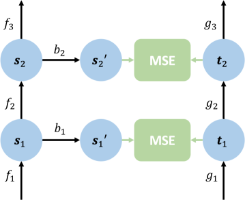
Figure 3: Adding a “bridge” to the structure. The bridge includes nonlinear layers to transform $s_{i}$ into $s_{i}^{\prime}$ such that $s_{i}^{\prime}\approx t_{i}$. The black arrows indicate the forward path.

A typical deep network training process requires features to pass through multiple nonlinear layers, allowing the output to approach the ground-truth labels. Therefore, there is only one objective. With AL, however, we modularize the training path by splitting it into smaller components and assign independent local objectives to each small component. Consequently, the AL technique divides the original long gradient flow into many independent short gradient flows and effectively eliminates the backward locking problem. In this section, we introduce three types of functions (associated function, encoding and decoding functions, and bridge function) that together compose the AL network.

4.1 Associated Function and Associated Loss

Referring to Figure 2, let $\boldsymbol{x}$ and $y$ be the input features and the output target, respectively, of a training sample. We split a network with $\ell$ hidden layers into $\ell/2$ components (assuming $\ell$ is an even number). The details of each component are illustrated in Figure 4. Each component $i$ consists of two local forward functions, $f_{i}$ and $g_{i}$ ($f_{i}$ and $g_{i}$ will be called the associated function and encoding function, respectively, for better differentiation; we will further explain the encoding function in Section 4.3), and a local objective function independent of the objective functions of the other components. A local associated function can be a simple single-layer perceptron, a convolutional layer, or another function. We compute $s_{i}$ using Equation 1:

$$s_{i}=f_{i}(s_{i-1}),\textrm{ }i=1,\ldots,\ell/2.$$ (1)

Note that here, $s_{0}$ equals $\boldsymbol{x}$.

We define the associated loss function for each pair of $(s_{i},t_{i})$ by Equation 2. This concept is similar to target propagation (Bengio, 2014; Lee et al., 2015; Bartunov et al., 2018), in which the goal is to minimize the distance between $s_{i}$ and $t_{i}$ for every component $i$.

$$L_{i}(s_{i},t_{i})=||s_{i}-t_{i}||^{2},\textrm{ }i=1,\ldots,\ell/2.$$ (2)

The optimizer in the $i^{\textrm{th}}$ component updates the parameters in $f_{i}$ to reduce the associated loss function (Equation 2).

Referring to Figure 2, Equation 2 attempts to make $\boldsymbol{s}_{i}\approx\boldsymbol{t}_{i}$ for all $i$. This design may look strange for several reasons. First, if we can obtain an $f_{1}$ such that $\boldsymbol{s}_{1}\approx\boldsymbol{t}_{1}$, all the other $f_{i}$s $(i>1)$ seem unnecessary. Second, since $\boldsymbol{s}_{1}$ and $\boldsymbol{t}_{1}$ are far apart, fitting these two terms seems counterintuitive.

For the first question, one can regard each component as one layer in a deep neural network. As we add more components, the corresponding $\boldsymbol{s}_{i}$ and $\boldsymbol{t}_{i}$ may become closer. For the second question, indeed, it seems more reasonable to fit the values of neighboring cells. However, our design breaks the gradient flow among different components so that it is possible to perform a parallel parameter update for each component.

4.2 Bridge Function

Our early experiments showed that $\boldsymbol{s}_{i}$ has difficulty fitting the corresponding target $\boldsymbol{t}_{i}$, especially for a convolutional neural network (CNN) and its variants. Thus, we insert nonlinear layers to improve the fitting between $\boldsymbol{s}_{i}$ and $\boldsymbol{t}_{i}$. As shown in Figure 3, we create a bridge function, $b_{i}$, to perform a nonlinear transform on $\boldsymbol{s}_{i}$ such that $b_{i}(\boldsymbol{s}_{i})=\boldsymbol{s}_{i}^{\prime}\approx\boldsymbol{t}_{i}$. As a result, the associated loss is reformulated to the following equation to replace the original Equation 2:

$$L_{i}(\boldsymbol{s}_{i},\boldsymbol{t}_{i})=||b_{i}(\boldsymbol{s}_{i})-\boldsymbol{t}_{i}||^{2},\textrm{ }i=1,\ldots,\ell/2,$$ (3)

where the function $b_{i}(.)$ serves as the bridge.

Although this approach greatly increases the number of parameters and the nonlinear layers to decrease the forward loss, except for the last bridge, these parameters do not affect the inference function, as we will explain in Section 4.5, so the bridges only slightly increase the hypothesis space. For a fair comparison, we also increase the number of parameters when the models are trained by BP so that the models trained by AL and trained by BP have the same number of parameters. The details will be explained in Section 5.

4.3 Encoding/Decoding Functions and Autoencoder Loss

Referring to Figure 2, in addition to the parameters of the $f_{i}$s and $b_{i}$s, we also need to obtain parameters in $h_{i}$s to have the mapping $\boldsymbol{t}_{i}\rightarrow\boldsymbol{t}_{i-1}$ at the inference phase. This mapping is achieved by the following two functions, which together can be regarded as an autoencoder:

$$\boldsymbol{t}_{i}=g_{i}(\boldsymbol{t}_{i-1}),~{}i=1,\ldots,\ell/2.$$ (4)

$$\boldsymbol{t}^{\prime}_{i-1}=h_{i}(\boldsymbol{t}_{i}),~{}i=i,\ldots,\ell/2.$$ (5)

Referring to Figure 4, the above two equations form an autoencoder because we want $\boldsymbol{t}_{i-1}\xrightarrow{g_{i}}\boldsymbol{t}_{i}\xrightarrow{h_{i}}\boldsymbol{t}_{i-1}^{\prime}\approx\boldsymbol{t}_{i-1}$, so $g_{i}$ and $h_{i}$ are called the encoding function and decoding function, respectively. The autoencoder loss $L^{\prime}_{i}$ for layer $i$ is defined by Equation 6:

$$L_{i}^{\prime}(h_{i}(g_{i}(\boldsymbol{t}_{i-1})),\boldsymbol{t}_{i-1})=||\boldsymbol{t}_{i-1}^{\prime}-\boldsymbol{t}_{i-1}||^{2},i=1,\ldots,\ell/2.$$ (6)

4.4 Putting Everything Together

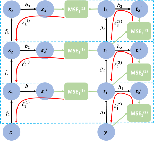
Figure 4: A training example using associated learning. The black arrows indicate the forward paths that involve learnable parameters; the green arrows connect the variables that should be compared to minimize their associated distance; the red arrows denote the backward gradient flows. We group each component by dashed lines. The parameters of the different components are independent so that they can be updated simultaneously. The variable $\ell_{u}^{(v)}$ denotes the $v$th gradient flow of the $u$th component. $\textrm{MSE}_{u}^{(v)}$ denotes the $v$th mean-squared error of the $u$th component. Consequently, the first gradient flow of each component, $\ell_{u}^{(1)}$, determines the updates of the parameters of $f_{u}$ and $b_{u}$; the second gradient flow of each component, $\ell_{u}^{(2)}$, determines the updates of $g_{u}$ and $h_{u}$.

Figure 4 shows the entire training process of AL based on our earlier example. We group each component by a dashed line. The parameters in each component are independent of the parameters in the other components. For each component $i$, the local objective function is defined by Equation 7.

$$\textrm{local-obj}_{i}=\textrm{MSE}_{i}^{(1)}+\textrm{MSE}_{i}^{(2)}=||b_{i}(\boldsymbol{s}_{i})-\boldsymbol{t}_{i}||^{2}+||\boldsymbol{t}_{i-1}^{\prime}-\boldsymbol{t}_{i-1}||^{2},$$ (7)

where $||b_{i}(\boldsymbol{s}_{i})-\boldsymbol{t}_{i}||^{2}$ is the associated loss shown by Equation 3 and $||\boldsymbol{t}_{i-1}^{\prime}-\boldsymbol{t}_{i-1}||^{2}$ is the autoencoder loss demonstrated by Equation 6.

As shown in Figure 4, the associated loss in each component creates the gradient flow $\ell_{i}^{(1)}$, which guides the updates of the parameters of $f_{i}$ and $b_{i}$. The autoencoder loss in each component leads to the second gradient flow $\ell_{i}^{(2)}$, which determines the updates of $g_{i}$ and $h_{i}$.

A gradient flow travels only within a component, so the parameters in different components can be updated simultaneously. Additionally, since each gradient flow is short, the vanishing gradient and exploding gradient problems are less likely to occur.

Since each component incrementally refines the association loss of the component immediately below it, the input $\boldsymbol{x}$ approaches the output $y$.

4.5 Inference Function, Effective Parameters, and Hypothesis Space

We can categorize the abovementioned parameters into two types: effective parameters and affiliated parameters. The affiliated parameters help the model determine the values of the effective parameters, which in turn determine the hypothesis space of the final inference function. Therefore, while increasing the number of affiliated parameters may help to obtain better values for the effective parameters, it will not increase the hypothesis space of the prediction model. Such a setting may be relevant to the overparameterization technique, which introduces redundant parameters to accelerate the training speed (Allen-Zhu et al., 2018; Arora et al., 2018; Chen, 2017; Chen and Chen, 2020), but here, the purpose is to obtain better values of the effective parameters rather than faster convergence.

Specifically, in the training phase, we search for the parameters of the $f_{i}$s and $b_{i}$s that minimize the associated loss and search for the parameters of the $g_{i}$s and $h_{i}$s to minimize the autoencoder loss. However, in the inference phase, we make predictions based only on Equation 1, Equation 5, and $b_{\ell/2}(\boldsymbol{s}_{\ell/2})$. Therefore, the effective parameters include only the parameters in the $f_{i}$s, the $h_{i}$s ($i=1,\ldots,\ell/2$), and $b_{\ell/2}$ (i.e., the last bridge). The parameters in the other functions (i.e., the $g_{i}$s $(i=1,\ldots,\ell/2)$ and the $b_{j}$s $(j=1,\ldots,\ell/2-1)$) are affiliated parameters; they do not increase the expressiveness of the model but only help determine the values of the effective parameters.

The predicting process can be represented in Figure 2. Equation 8 shows the prediction function:

$$\hat{y}=\left(h_{1}\circ h_{2}\circ\ldots\circ h_{\ell/2}\circ b_{\ell/2}\circ f_{\ell/2}\circ\ldots\circ f_{2}\circ f_{1}\right)(\boldsymbol{x}),$$ (8)

where $\circ$ denotes the function composition operation and $\ell=6$ in the example is illustrated by Figure 2 and Figure 4. Only the parameters involved in Equation 8 are the effective parameters that determine the hypothesis space.

5 Experiments

In this section, we introduce the experimental settings, implementation details, and show the results of the performance comparisons between BP and AL.

5.1 Experimental Settings

We conducted experiments by applying AL and BP to different deep neural network structures (a multilayer perceptron (MLP), a vanilla CNN, a Visual Geometry Group (VGG) network (Simonyan and Zisserman, 2015), a 20-layer residual neural network (ResNet-20), and a 32-layer ResNet (ResNet-32) (He et al., 2016)) and different datasets (the Modified National Institute of Standards and Technology (MNIST) (LeCun et al., 1998), the 10-class Canadian Institute for Advanced Research (CIFAR-10), and the 100-class CIFAR (CIFAR-100) (Krizhevsky and Hinton, 2009) datasets). Surprisingly, although the AL approach aims at minimizing the local losses, its prediction accuracy is comparable to, and sometimes even better than, that of BP-based learning, whose goal is directly minimizing the prediction error.

In each experiment, we used the settings that were reported in recent papers. We spent a reasonable amount of time searching for the hyperparameters not stated in previous papers based on random search (Bergstra and Bengio, 2012). Eventually, we initialized all the weights based on the He normal initializer and use Adam as the optimizer. We experimented with different activation functions and adopted the exponential linear unit (ELU) for all the local forward functions (i.e., $f_{i}$) and a sigmoid function for the functions related to the autoencoders and bridges (i.e., $g_{i}$, $h_{i}$, and $b_{i}$). The models trained by BP yielded test accuracies close to the state-of-the-art (SOTA) results under the same or similar network structures (He et al., 2016; Carranza-Rojas et al., 2019). In addition, because AL includes extra parameters in the function $b_{\ell/2}$ (the last bridge), as explained in Section 4.5, we increased the number of layers in the corresponding baseline models when training by BP so that the models trained by AL and those trained by BP have identical parameters, so the comparisons are fair.

The implementations are freely available at https://github.com/SamYWK/Associated_Learning.

5.2 Test Accuracy

Table 2: Test accuracy comparison on the MNIST dataset. We highlight the winner in bold font. We applied only the DTP algorithm on the MLP because this is the setting used in the original paper. Applying DTP on other networks might require different designs.

	BP	AL	DTP
MLP	$98.5\pm 0.0\%$	$\boldsymbol{98.6\pm 0.0\%}$	$96.43\pm 0.04\%$
Vanilla CNN	$99.4\pm 0.0\%$	$\boldsymbol{99.5\pm 0.0\%}$	-

To test the capability of AL, we compared AL and BP on different network structures (MLP, vanilla CNN, ResNet, and VGG) and different datasets (MNIST, CIFAR-10, and CIFAR-100). When converting a network with an odd number of layers into the ”folded” architecture used by AL, the middle layer is simply absorbed by the bridge layer at the top component shown in Figure 4. We also experimented with differential target propagation (DTP) (Lee et al., 2015) on the MLP network based on the MNIST dataset. We tried only the MLP network, as the original paper applied only DTP to the MLP structure and applying DTP to other network structures requires different designs.

On the MNIST dataset, we conducted experiments with only two networks structures, MLP and vanilla CNN, because using even these simple structures yielded decent test accuracies. Their detailed settings are described in the following paragraphs. The results are shown in Table 2. For both the MLP and the vanilla CNN structure, AL performs slightly better than BP, which performs better than DTP on the MLP network.

The MLP contains 5 hidden layers and 1 output layer; there are $1024$, $1024$, $5120$, $1024$, and $1024$ neurons in the hidden layers and $10$ neurons in the output layer. Referring to Figure 4, this network corresponds to the following structure when using the AL framework: the network has two components; both the $\boldsymbol{s}_{i}$ and $\boldsymbol{t}_{i}$ in a component $i$ ($i=1,2$) have $1024$ neurons, and $\boldsymbol{b}_{2}$ the output of the top bridge function contains $5120$ neurons.

The vanilla CNN contains 13 hidden layers and 1 output layer. The first 4 layers are convolutional layers with a size of $3\times 3\times 32$ (i.e., a width of 3, a height of 3, and 32 kernels) in each layer, followed by 4 convolutional layers with a size of $3\times 3\times 64$ in each layer, followed by a fully connected layer with $1280$ neurons, followed by 4 fully connected layers with $256$ neurons in each layer and ending with a fully connected layer with 10 neurons. When training by AL, this structure corresponds to the following: the first five layers (layers 1 to 5) and the last five layers (layers 9 to 13) form five components, where layer $i$ and layer $14-i$ ($i=1,\ldots,5$) belong to component $i$ and the $6^{\textrm{th}}$, $7^{\textrm{th}}$, and $8^{\textrm{th}}$ layers construct the component $6$. The initial learning rate is $10^{-4}$, which is reduced after $80$, $120$, $160$, and $180$ epochs.

Table 3: Test accuracy comparison on the CIFAR-10 dataset. We highlight the winner in bold font. We applied only the DTP algorithm on the MLP because this is the setting used in the original paper. Applying DTP on other networks might require different designs.

	BP	AL	DTP
MLP	$60.6\pm 0.3\%$	$\boldsymbol{62.8\pm 0.2\%}$	$58.2\pm 0.2\%$
Vanilla CNN	$85.2\pm 0.4\%$	$\boldsymbol{85.8\pm 0.1\%}$	-
ResNet-20	$\boldsymbol{91.2\pm 0.4\%}$	$89.1\pm 0.5\%$	-
ResNet-32	$\boldsymbol{92.0\pm 0.2\%}$	$88.7\pm 0.4\%$	-
VGG	$92.3\pm 0.2\%$	$\boldsymbol{92.6\pm 0.1\%}$	-

Table 4: Test accuracy comparison on the CIFAR-100 dataset. We highlight the winner in bold font.

	BP	AL
MLP	$26.5\pm 0.4\%$	$\boldsymbol{29.7\pm 0.2\%}$
Vanilla CNN	$51.1\pm 0.2\%$	$\boldsymbol{52.2\pm 0.5\%}$
ResNet-20	$\boldsymbol{63.7\pm 0.2\%}$	$61.0\pm 0.6\%$
ResNet-32	$\boldsymbol{63.7\pm 0.3\%}$	$59.0\pm 1.6\%$
VGG	$65.8\pm 0.3\%$	$\boldsymbol{67.1\pm 0.3\%}$

The CIFAR-10 dataset is more challenging than the MNIST dataset. The input image size is $32\times 32\times 3$ (Krizhevsky and Hinton, 2009); i.e., the images have a higher resolution, and each pixel includes red, green, and blue (RGB) information. To make good use of these abundant features, we included not only MLP and vanilla CNN in this experiment but also VGG and the ResNets. The input images are augmented by 2-pixel jittering (Sabour et al., 2017). We applied the L2-norm using $5\times 10^{-4}$ and $1\times 10^{-4}$ as the regularization weights for VGG and the ResNet models.

Because ResNet uses batch normalization and the shortcut trick, we set its learning rate to $10^{-3}$, which slightly larger than that of the other models. In addition, to ensure that the models trained by BP and AL have identical numbers of parameters for a fair comparison, we added extra layers to ResNet-20, ResNet-32, and VGG when using BP for learning.

Table 3 shows the results of the CIFAR-10 dataset. AL performs marginally better than BP on the MLP, vanilla CNN, and VGG structures. With the ResNet structure, AL performs slightly worse than BP. The CIFAR-100 dataset includes 100 classes. We used model settings that were nearly identical to the settings used on the CIFAR-10 dataset but increased the number of neurons in the bridge. Table 4 shows the results. As in CIFAR-10, AL performs better than BP on the MLP, vanilla CNN, and VGG structures but slightly worse on the ResNet structures.

Currently, the theoretical aspects of the AL method are weak, so we are unsure of the fundamental reasons why AL outperforms BP on MLP, vanilla CNN, and VGG but BP outperforms AL on ResNet. Our speculations are below. First, since BP aims to fit the target directly, and most of the layers in AL can leverage only indirect clues to update the parameters, AL is less likely to outperform BP. However, this reason does not explain why AL performs better than BP on other networks. Second, perhaps the bridges can be regarded implicitly as the shortcut connections of ResNet, so applying AL on ResNet appears such as refining residuals of residuals, which could be noisy. Finally, years of study on BP has made us gain experience on the hyperparameter settings for BP. A similar hyperparameter setting may not necessarily achieve the best setting for AL.

As reported in (Bartunov et al., 2018), earlier studies on BP alternatives, such as target propagation (TP) and feedback alignment (FA), performed worse than BP in non-fully connected networks (e.g., a locally connected network such as a CNN) and more complex datasets (e.g., CIFAR). Recent studies, such as those on decoupled greedy learning (DGL) and the Predsim model (Belilovsky et al., 2019; Nøkland and Eidnes, 2019), showed a similar performance to BP on more complex networks, e.g., VGG, but these models require each layer to access the target label $y$ directly, which could be biologically implausible because distant neurons are unlikely to obtain the signals directly from the target. As far as we know, our proposed AL technique is the first work to show that an alternative of BP works on various network structures without directly revealing the target $y$ to each hidden layer, and the results are comparable to, and sometimes even better than, the networks trained by BP.

5.3 Number of Layers vs. the Associated Loss and vs. the Accuracy

Table 5: The associated loss at different layers on the MNIST dataset after 200 epochs. Referring to Figure 4, for each layer, its corresponding $\boldsymbol{s}_{i}$ and $\boldsymbol{t}_{i}$ both contain $1024$ neurons.

Number of component layers	1 layer	2 layers	3 layers
$||\boldsymbol{s}_{1}^{\prime}-\boldsymbol{t}_{1}||_{2}^{2}$	$1.2488\times 10^{-5}$	$1.5469\times 10^{-5}$	$1.2219\times 10^{-5}$
$||\boldsymbol{s}_{2}^{\prime}-\boldsymbol{t}_{2}||_{2}^{2}$	-	$3.5818\times 10^{-7}$	$3.8033\times 10^{-7}$
$||\boldsymbol{s}_{3}^{\prime}-\boldsymbol{t}_{3}||_{2}^{2}$	-	-	$6.7192\times 10^{-10}$

Table 6: Number of layers vs. the training accuracy and vs. the test accuracy on the MNIST dataset after 200 epochs. Referring to Figure 4, for each layer, the corresponding $\boldsymbol{s}_{i}$ and $\boldsymbol{t}_{i}$ both contain $1024$ neurons. The bridge layer in the top layer includes $5120$ neurons.

Number of component layers	1 layer	2 layers	3 layers
Training accuracy	1.0	1.0	1.0
Test accuracy	0.9849	0.9860	0.9871

This section presents the results of experiments with different numbers of component layers on the MNIST dataset. For each component layer $i$, both the corresponding $\boldsymbol{s}_{i}$ and $\boldsymbol{t}_{i}$ have $1024$ neurons, and $\boldsymbol{s}^{\prime}_{\ell}$ (i.e., the output of the bridge at the top layer) contains $5120$ neurons.

First, we show that each component indeed incrementally refines the associated loss of the one immediately below it. Specifically, we applied AL to the MLP and experimented with different numbers of component layers. As shown in Table 5, adding more layers truly decreases the associated loss, and the associated loss at an upper layer is smaller than that at a lower layer.

Second, we show that adding more layers helps transform $\boldsymbol{x}$ into $y$. As shown in Table 6, adding more layers increases the test accuracy.

5.4 Metafeature Visualization and Quantification

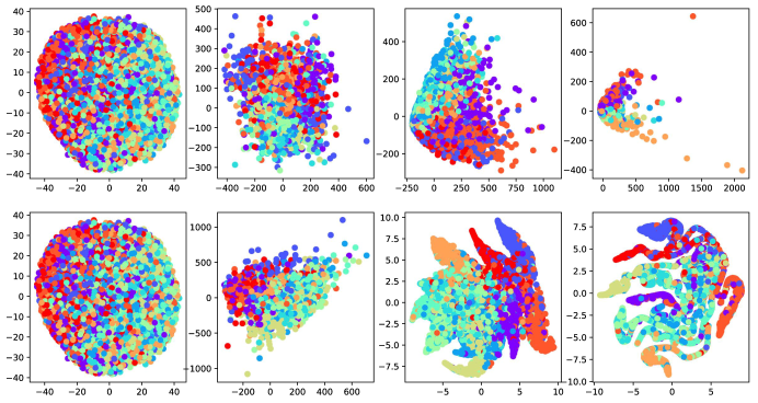
Figure 5: t-SNE visualization of the MLP on the CIFAR-10 dataset. The different colors represent different labels. The figures in the first row are the results of the raw data, $2^{\textrm{nd}}$ layer, $4^{\textrm{th}}$ layer, and output layer when using BP. The second row shows the corresponding results for AL.

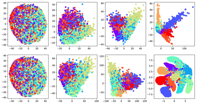
Figure 6: t-SNE visualization of Vanilla CNN with CIFAR-10 dataset. The different colors represent different labels. The figures in the first row are the results of the raw data, $4^{\textrm{th}}$ layer, $8^{\textrm{th}}$ layer, and $12^{\textrm{th}}$ layers when using BP. The second row shows the corresponding results for AL.

Table 7: A comparison of the inter- and intraclass distances and the ratio of the two. We highlight the winner in bold font.

Dataset	Network	Method	Interclass distance	Intraclass distance	Inter:Intra ratio
CIFAR-10	MLP	BP	$39.36$	$67.97$	$0.58$
		AL	$0.73$	$0.66$	$\boldsymbol{1.11}$
	Vanilla CNN	BP	$41.82$	$26.87$	$1.56$
		AL	$1.17$	$0.36$	$\boldsymbol{3.25}$
CIFAR-100	MLP	BP	$114.42$	$342.65$	$0.33$
		AL	$0.23$	$0.28$	$\boldsymbol{0.82}$
	Vanilla CNN	BP	$114.71$	$163.43$	$0.70$
		AL	$0.55$	$0.51$	$\boldsymbol{1.08}$

To determine whether the hidden layers truly learn useful metafeatures when using AL, we used t-SNE (Maaten and Hinton, 2008) to visualize the $2^{\textrm{nd}}$, $4^{\textrm{th}}$ hidden layers and output layer in the 6-layer MLP model and the $4^{\textrm{th}}$, $8^{\textrm{th}}$, and $12^{\textrm{th}}$hidden layers in the 14-layer Vanilla CNN model on the CIFAR-10 dataset. For comparison purposes, we also visualize the corresponding hidden layers trained using BP. As shown in Figure 5 and Figure 6, the initial layers seem to extract less useful metafeatures than the later layers because the labels are difficult to distinguish in the corresponding figures. However, a comparison of the last few layers shows that AL groups the data points of the same label more accurately than BP, which suggests that AL likely learns better metafeatures.

To assess the quality of the learned metafeatures, we calculated the intra- and interclass distances of the data points based on the metafeatures. We computed the intraclass distance $d_{k}^{intra}$ as the average distance between any two data points in class $k$ for each class. The interclass distance is the average distance between the centroids of the classes. We also computed the ratio between inter- and intraclass distance to determine the quality of the metafeatures generated by AL and BP (Michael and Lin, 1973; Luo et al., 2019). As shown in Table 7, AL performs better than BP on both the CIFAR-10 and CIFAR-100 datasets because AL generates metafeatures with a larger ratio between inter- and intraclass distance.

6 Discussion and Future Work

Although BP is the cornerstone of today’s deep learning algorithms, it is far from ideal, and therefore, improving BP or searching for alternatives is an important research direction. This paper discusses AL, a novel process for training deep neural networks without end-to-end BP. Rather than calculating gradients in a layerwise fashion based on BP, AL removes the dependencies between the parameters of different subnetworks, thus allowing each subnetwork to be trained simultaneously and independently. Consequently, we may utilize pipelines to increase the training throughput. Our method is biologically plausible because the targets are local and the gradients are not obtained from the output layer. Although AL does not directly minimize the prediction error, its test accuracy is comparable to, and sometimes better than, that of BP, which does directly attempt to minimize the prediction error. Although recent studies have begun to use local losses instead of backpropagating the global loss (Nøkland and Eidnes, 2019), these local losses are computed mainly based on (or are at least partially based on) the difference between the target variable and the predicted results. Our method is unique because in AL, most of the layers do not interact with the target variable.

Current strategies to parallelize the training of a deep learning model usually distribute the training data into different computing units and aggregate (e.g., by averaging) the gradients computed by each computing unit. Our work, on the other hand, parallelizes the training step by computing the parameters of the different layers simultaneously. Therefore, AL is not an alternative to most of the other parallel training approaches but can integrate with the abovementioned approach to further improve the training throughput.

Years of research have allowed us to gradually understand the proper hyperparameter settings (e.g., network structure, weight initialization, and activation function) when training a neural network based on BP. However, these settings may not be appropriate when training by AL. Therefore, one possible research direction is to search for the right settings for this new approach.

We implemented AL in TensorFlow. However, we were unable to implement the “pipelined” AL that was shown in Table 1 within a reasonable period because of the technical challenges of task scheduling and parallelization in TensorFlow. We decided to leave this part as future work. However, we ensure that the gradients propagate only within each component, so theoretically, a pipelined AL should be able to be implemented.

Another possible future work is validating AL on other datasets. (e.g., ImageNet, Microsoft Common Objects in Context (MS COCO), and Google’s Open Images) and even on datasets unrelated to computer vision, such as those used in signal processing, natural language processing, and recommender systems. Yet another future work is the theoretical work of AL, as this may help us understand why AL outperforms BP under certain network structures. In the longer term, we are highly interested in investigating optimization algorithms beyond BP and gradients.

Acknowledgments

We acknowledge partial support by the Ministry of Science and Technology under grant no. MOST 107-2221-E-008-077-MY3. We thank the reviewers for their informative feedback.

References

- Allen-Zhu et al. (2018) Allen-Zhu, Z., Li, Y., and Song, Z. (2018). A convergence theory for deep learning via over-parameterization. arXiv preprint arXiv:1811.03962.
- Arora et al. (2018) Arora, S., Cohen, N., and Hazan, E. (2018). On the optimization of deep networks: implicit acceleration by overparameterization. arXiv preprint arXiv:1802.06509.
- Baldi (2012) Baldi, P. (2012). Autoencoders, unsupervised learning, and deep architectures. In Proceedings of ICML workshop on unsupervised and transfer learning, pages 37–49.
- Balduzzi et al. (2015) Balduzzi, D., Vanchinathan, H., and Buhmann, J. M. (2015). Kickback cuts backprop’s red-tape: biologically plausible credit assignment in neural networks. In Proceedings of the Twenty-Ninth AAAI Conference on Artificial Intelligence, pages 485–491.
- Bartunov et al. (2018) Bartunov, S., Santoro, A., Richards, B., Marris, L., Hinton, G. E., and Lillicrap, T. (2018). Assessing the scalability of biologically-motivated deep learning algorithms and architectures. In Advances in Neural Information Processing Systems, pages 9390–9400.
- Belilovsky et al. (2018) Belilovsky, E., Eickenberg, M., and Oyallon, E. (2018). Greedy layerwise learning can scale to imagenet. arXiv preprint arXiv:1812.11446.
- Belilovsky et al. (2019) Belilovsky, E., Eickenberg, M., and Oyallon, E. (2019). Decoupled greedy learning of CNNs. arXiv preprint arXiv:1901.08164.
- Bengio (2014) Bengio, Y. (2014). How auto-encoders could provide credit assignment in deep networks via target propagation. arXiv preprint arXiv:1407.7906.
- Bengio et al. (2015) Bengio, Y., Lee, D.-H., Bornschein, J., Mesnard, T., and Lin, Z. (2015). Towards biologically plausible deep learning. arXiv preprint arXiv:1502.04156.
- Bergstra and Bengio (2012) Bergstra, J. and Bengio, Y. (2012). Random search for hyper-parameter optimization. Journal of Machine Learning Research, 13(Feb):281–305.
- Carranza-Rojas et al. (2019) Carranza-Rojas, J., Calderon-Ramirez, S., Mora-Fallas, A., Granados-Menani, M., and Torrents-Barrena, J. (2019). Unsharp masking layer: injecting prior knowledge in convolutional networks for image classification. In International Conference on Artificial Neural Networks, pages 3–16. Springer.
- Chen (2017) Chen, H.-H. (2017). Weighted-svd: matrix factorization with weights on the latent factors. arXiv preprint arXiv:1710.00482.
- Chen and Chen (2020) Chen, P. and Chen, H.-H. (2020). Accelerating matrix factorization by overparameterization. In International Conference on Deep Learning Theory and Applications, pages 89–97.
- Crick (1989) Crick, F. (1989). The recent excitement about neural networks. Nature, 337(6203):129–132.
- He et al. (2016) He, K., Zhang, X., Ren, S., and Sun, J. (2016). Deep residual learning for image recognition. In Proceedings of the IEEE Conference on Computer Vision and Pattern Recognition, pages 770–778.
- Hochreiter and Schmidhuber (1997) Hochreiter, S. and Schmidhuber, J. (1997). Long short-term memory. Neural Computation, 9(8):1735–1780.
- Huang et al. (2019) Huang, Y., Cheng, Y., Bapna, A., Firat, O., Chen, D., Chen, M., Lee, H., Ngiam, J., Le, Q. V., Wu, Y., et al. (2019). Gpipe: efficient training of giant neural networks using pipeline parallelism. In Advances in Neural Information Processing Systems, pages 103–112.
- Huo et al. (2018a) Huo, Z., Gu, B., and Huang, H. (2018a). Training neural networks using features replay. In Advances in Neural Information Processing Systems, pages 6659–6668.
- Huo et al. (2018b) Huo, Z., Gu, B., Yang, Q., and Huang, H. (2018b). Decoupled parallel backpropagation with convergence guarantee. arXiv preprint arXiv:1804.10574.
- Jaderberg et al. (2016) Jaderberg, M., Czarnecki, W. M., Osindero, S., Vinyals, O., Graves, A., Silver, D., and Kavukcuoglu, K. (2016). Decoupled neural interfaces using synthetic gradients. arXiv preprint arXiv:1608.05343.
- Krizhevsky and Hinton (2009) Krizhevsky, A. and Hinton, G. (2009). Learning multiple layers of features from tiny images. Technical report, University of Toronto.
- LeCun et al. (1998) LeCun, Y., Bottou, L., Bengio, Y., and Haffner, P. (1998). Gradient-based learning applied to document recognition. Proceedings of the IEEE, 86(11):2278–2324.
- Lee et al. (2015) Lee, D.-H., Zhang, S., Fischer, A., and Bengio, Y. (2015). Difference target propagation. In Joint European Conference on Machine Learning and Knowledge Discovery in Databases, pages 498–515. Springer.
- Lillicrap et al. (2016) Lillicrap, T. P., Cownden, D., Tweed, D. B., and Akerman, C. J. (2016). Random synaptic feedback weights support error backpropagation for deep learning. Nature Communications, 7:13276.
- Luo et al. (2019) Luo, Y., Wong, Y., Kankanhalli, M., and Zhao, Q. (2019). G-softmax: improving intraclass compactness and interclass separability of features. IEEE Transactions on Neural Networks and Learning Systems.
- Maaten and Hinton (2008) Maaten, L. v. d. and Hinton, G. (2008). Visualizing data using t-sne. Journal of Machine Learning Research, 9(Nov):2579–2605.
- Michael and Lin (1973) Michael, M. and Lin, W.-C. (1973). Experimental study of information measure and inter-intra class distance ratios on feature selection and orderings. IEEE Transactions on Systems, Man, and Cybernetics, pages 172–181.
- Mostafa et al. (2018) Mostafa, H., Ramesh, V., and Cauwenberghs, G. (2018). Deep supervised learning using local errors. Frontiers in Neuroscience, 12:608.
- Nøkland (2016) Nøkland, A. (2016). Direct feedback alignment provides learning in deep neural networks. In Advances in Neural Information Processing Systems, pages 1037–1045.
- Nøkland and Eidnes (2019) Nøkland, A. and Eidnes, L. H. (2019). Training neural networks with local error signals. arXiv preprint arXiv:1901.06656.
- Ororbia and Mali (2019) Ororbia, A. G. and Mali, A. (2019). Biologically motivated algorithms for propagating local target representations. In Proceedings of the AAAI conference on artificial intelligence, volume 33, pages 4651–4658.
- Ororbia et al. (2018) Ororbia, A. G., Mali, A., Kifer, D., and Giles, C. L. (2018). Conducting credit assignment by aligning local representations. arXiv preprint arXiv:1803.01834.
- Rumelhart et al. (1986) Rumelhart, D. E., Hinton, G. E., and Williams, R. J. (1986). Learning representations by back-propagating errors. Nature, 323(6088):533.
- Sabour et al. (2017) Sabour, S., Frosst, N., and Hinton, G. E. (2017). Dynamic routing between capsules. In Advances in Neural Information Processing Systems, pages 3856–3866.
- Shallue et al. (2018) Shallue, C. J., Lee, J., Antognini, J., Sohl-Dickstein, J., Frostig, R., and Dahl, G. E. (2018). Measuring the effects of data parallelism on neural network training. arXiv preprint arXiv:1811.03600.
- Simonyan and Zisserman (2015) Simonyan, K. and Zisserman, A. (2015). Very deep convolutional networks for large-scale image recognition. In International Conference on Learning Representations.
- Taylor et al. (2016) Taylor, G., Burmeister, R., Xu, Z., Singh, B., Patel, A., and Goldstein, T. (2016). Training neural networks without gradients: a scalable admm approach. In International Conference on Machine Learning, pages 2722–2731.
- Zinkevich et al. (2010) Zinkevich, M., Weimer, M., Li, L., and Smola, A. J. (2010). Parallelized stochastic gradient descent. In Advances in Neural Information Processing Systems, pages 2595–2603.