Interpretable ICD Code Embeddings with Self- and Mutual-Attention Mechanisms

Abstract

We propose a novel and interpretable embedding method to represent the international statistical classification codes of diseases and related health problems ($i.e.$, ICD codes). This method considers a self-attention mechanism within the disease domain and a mutual-attention mechanism jointly between diseases and procedures. This framework captures the clinical relationships between the disease codes and procedures associated with hospital admissions, and it predicts procedures according to diagnosed diseases. A self-attention network is learned to fuse the embeddings of the diseases for each admission. The similarities between the fused disease embedding and the procedure embeddings indicate which procedure should potentially be recommended. Additionally, when learning the embeddings of the ICD codes, the optimal transport between the diseases and the procedures within each admission is calculated as a regularizer of the embeddings. The optimal transport provides a mutual-attention map between diseases and the procedures, which suppresses the ambiguity within their clinical relationships. The proposed method achieves clinically-interpretable embeddings of ICD codes, and outperforms state-of-the-art embedding methods in procedure recommendation.

1 Introduction

The International Classification of Diseases (ICD) is provided by the World Health Organization (WHO), and contains codes for diseases, procedures, and external causes of injury or disease. ICD codes play an important role in patient electrical health records (EHRs). For example, the hospital admission of a patient is often summarized as a set of disease ICD codes and a set of procedure ICD codes. The disease ICD codes represent the diagnosis provided by doctors, and the procedure ICD codes indicate the treatments applied to the patient.

A significant and interesting problem is predicting procedures given diagnosed diseases, which can be useful for improving the effectiveness and the efficiency of hospital admission. From the viewpoint of machine learning, this problem can be formulated as an ICD code embedding task. Specifically, given a patient admission record, we aim to represent the ICD codes of the diseases and procedures appearing in the record as embedding vectors. Accordingly, one may anticipate a procedure for a given disease when the two have similar embedding vectors.

Unfortunately, most existing embedding methods may not be suitable for the proposed problem because of the special properties of ICD codes. For each admission, the corresponding disease ICD codes and procedure ICD codes are ranked according to a manually-defined priority, rather than their real clinical relationships. Additionally, a disease often leads to multiple procedures and a procedure may correspond to multiple diseases. In other words, the diseases and the procedures in an admission often have complicated clinical relationships, but the mapping between these two code sets is unavailable. Such uncertainties in the admission records are challenging for existing embedding methods, because they require well-structured observations, $e.g.$, sequential data like words in sentences (Mikolov et al., 2013; Pennington et al., 2014), pairwise interactions like user-item pairs in recommender systems (Rendle et al., 2009; Chen et al., 2018a), and node interactions in graphs (Perozzi et al., 2014; Tang et al., 2015; Grover and Leskovec, 2016). As a result, applying existing methods to embed ICD codes directly suffers from a high risk of model misspecification. Moreover, like other clinical data analysis tasks (Choi et al., 2016a; Mullenbach et al., 2018; Mahmood et al., 2018), the proposed embeddings of ICD codes should be interpretable, $e.g.$, it is desirable that the clinical relationships between diseases and procedures can be explicitly captured by the distance/similarity between their embedding vectors. Although some existing embedding methods can capture simple pairwise relationships between their embedded entities, it is still difficult to describe more complicated relationships among multiple entities.

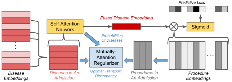
Figure 1: Scheme of proposed method. The mutual-attention module and the blue arrows are only used in the training phase. The remaining modules and the black arrows are used in both the training and testing phases.

Focusing on the challenges of ICD code embeddings, we propose an interpretable embedding method with novel self- and mutual-attention mechanisms. As illustrated in Figure 1, our method contains a self-attention network to fuse observed disease embeddings together. Accordingly, the similarity between the fused disease embedding and each procedure embedding is calculated, and procedures with high similarity are predicted to fit the observed procedures. When learning the embeddings and the self-attention network, we take advantage of the optimal-transport distance (Villani, 2008) between observed diseases and procedures as the regularizer of our model, achieving a mutual-attention map between them. The self- and the mutual-attention mechanisms are connected via the estimated probabilities of diseases. The proposed method has the advantages of interpretability of learned embeddings. Specifically, for each admission, the self-attention network estimates the probabilities of observed diseases, which can be interpreted as the significance of the disease in the admission. Additionally, the mutual-attention regularizer estimates the optimal transport between the observed diseases and procedures, which estimates their clinical relationships.

The proposed method can be used to recommend suitable procedures according to diagnosed diseases, which can be used to improve the efficiency of hospital admission, $i.e.$, for some typical diseases, clinicians, especially those junior and with limited clinical experience, can query suitable procedures quickly. Additionally, the recommended procedure codes can help to double-check the codes entered by clinicians.For other clinical data analysis tasks like ICD code assignment (Baumel et al., 2017; Huang et al., 2018), which requires ICD code embeddings as the input of down-stream models and applications, the proposed embeddings generated by our method can either provide high-quality inputs or improve the training of their ICD code embeddings via good initialization.

2 Target Data Set and Problem Statement

The proposed work employs the publicly-available MIMIC-III dataset (Johnson et al., 2016), developed by the MIT Lab for Computational Physiology. It comprises over 58,000 hospital admissions recorded from June 2001 to October 2012 for 38,645 adults and 7,875 neonates. For each admission, its ICD codes are generated for billing purposes at the end of the hospital stay, which includes a set of disease ICD codes and a set of procedure ICD codes. The ICD codes employ the ICD-9 format. In the MIMIC-III dataset, 14,567 disease ICD codes and 3,882 procedure ICD codes are observed. Each admission contains 1 to 41 diseases and 1 to 40 procedures.

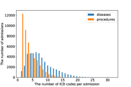
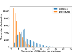
[Small set] [Medium set] [Large set]

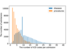
Figure 2: Histograms of admissions, with respect to the number of diseases (blue) and procedures (orange) per admission for the three subsets.

We consider three subsets of the MIMIC-III dataset. For each subset, we select the admissions having non-empty diseases and procedures. The small dataset contains 28,315 admissions with 247 diseases and 75 procedures, and each ICD code appears at least 500 times. The medium dataset contains 30,555 admissions with 874 diseases and 258 procedures, and each ICD code appears at least 100 times. The large dataset contains 31,213 admissions with 2,765 diseases and 819 procedures, and each ICD code appears at least 10 times. For these three subsets, the histograms of admissions with respect to the number of diseases and that of procedures are shown in Figure 2. We find that the histograms of admissions corresponding to the number of procedure ICD code per admission are consistent across different subsets, implying that the empirical distribution of procedures is stable and may yield an exponential distribution. On the other hand, the histograms of admissions with respect to the number of diseases per admission have changes with the increase of data size.

We denote the set of disease and procedure ICD codes as $\mathcal{D}=\{d_{1},d_{2},...\}$ and $\mathcal{P}=\{p_{1},p_{2},...\}$, respectively, where the sizes of the two sets are $|\mathcal{D}|$ and $|\mathcal{P}|$. Each element $d\in\mathcal{D}$ represents a specific disease and each $p\in\mathcal{P}$ represents a specific procedure. Suppose that we observed $I$ hospital admissions. For the $i$-th admission, $i\in\{1,...,I\}$, the diseases and the procedures associated with the admission are denoted $\mathcal{D}_{i}$ and $\mathcal{P}_{i}^{+}$, respectively. Here, $\mathcal{P}_{i}^{+}$ contains the “positive” procedures corresponding to $\mathcal{D}_{i}$. Accordingly, we can define/generate “negative” procedures that are potentially irrelevant to $\mathcal{D}_{i}$, $i.e.$, $\mathcal{P}_{i}^{-}\subset\mathcal{P}\setminus\mathcal{P}_{i}^{+}$, used in the following learning algorithm.

Given such observations, we aim to $i$) embed ICD codes of diseases and procedures; $ii$) predict reasonable procedures from diagnosed diseases according to proposed embeddings; and $iii$) it is desired that the prediction is clinically-interpretable. In the following sections, we denote the embeddings of diseases and procedures as $\bm{U}=[\bm{u}_{d}]\in\mathbb{R}^{M\times|\mathcal{D}|}$ and $\bm{V}=[\bm{v}_{p}]\in\mathbb{R}^{M\times|\mathcal{P}|}$, respectively, where $M$ is the embedding dimension.

3 Proposed Model and Learning Algorithm

3.1 Predicting procedures from diseases

Our embedding method learns a predictive model of procedures. For the $i$-th admission, we predict the set of procedures $\mathcal{P}_{i}^{+}$ from the set of diseases $\mathcal{D}_{i}$. Specifically, for each procedure $p\in\mathcal{P}$, we represent the probability of $p$ conditioned on $\mathcal{D}_{i}$ via the following parametric model:

$$\begin{aligned} \mbox{Prob}_{\theta}(p|\mathcal{D}_{i})=\mbox{sigmoid}(\bm{v}_{p}^{\top}f(\bm{U}_{\mathcal{D}_{i}})),~{}\forall~{}p\in\mathcal{P}.\end{aligned}$$ (1)

where $\bm{v}_{p}\in\mathbb{R}^{M}$ is the embedding of the procedure $p$, $\bm{U}_{\mathcal{D}_{i}}=[\bm{u}_{d}]_{d\in\mathcal{D}_{i}}\in\mathbb{R}^{M\times|\mathcal{D}_{i}|}$ contains the columns of $\bm{U}$ corresponding to $\mathcal{D}_{i}$, and $f(\cdot)$ is a function fusing columns of $\bm{U}_{\mathcal{D}_{i}}$ to a single vector. For convenience, we denote the parameters of the predictive model as $\theta=\{\bm{U}\in\mathbb{R}^{M\times|\mathcal{D}|},~{}\bm{V}\in\mathbb{R}^{M\times|\mathcal{P}|},~{}f(\cdot)\}$.

For the positive procedure $p\in\mathcal{P}_{i}^{+}$, it is desirable that the proposed model makes $\mbox{Prob}_{\theta}(p|\mathcal{D}_{i})$ approach $1$. By contrast, for the negative procedure $p\in\mathcal{P}\setminus\mathcal{P}_{i}^{+}$, the proposed model should suppress $\mbox{Prob}_{\theta}(p|\mathcal{D}_{i})$ to $0$. It should be noted that for each admission the number of negative procedures is much larger than that of positive procedures ($i.e.$, $|\mathcal{P}\setminus\mathcal{P}_{i}^{+}|\gg|\mathcal{P}_{i}^{+}|$). Therefore, in practice we must apply the negative sampling strategy used in other embedding methods (Rendle et al., 2009; Mikolov et al., 2013), randomly selecting a subset of negative procedures, $i.e.$, $\mathcal{P}_{i}^{-}\subset\mathcal{P}\setminus\mathcal{P}_{i}^{+}$ and ensuring $|\mathcal{P}_{i}^{-}|=|\mathcal{P}_{i}^{+}|$.

Accordingly, we can learn the model via maximum likelihood estimation (MLE): for the $i$-th admission, its predictive loss is

$$\begin{aligned} L_{P}(\mathcal{D}_{i},\mathcal{P}_{i}^{+},\mathcal{P}_{i}^{-};\theta)=-\sideset{}{{}_{p\in\mathcal{P}_{i}^{+}}}{\sum}\log\mbox{Prob}_{\theta}(p|\mathcal{D}_{i})-\sideset{}{{}_{p\in\mathcal{P}_{i}^{-}}}{\sum}\log(1-\mbox{Prob}_{\theta}(p|\mathcal{D}_{i})).\end{aligned}$$ (2)

By minimizing $L_{P}$, we maximize the log-likelihood of the observed procedures given the corresponding diagnosed diseases, and suppress the log-likelihood of the irrelevant procedures.

3.2 Fusing disease embeddings with a self-attention mechanism

The key of the above predictive model is the fusion function $f(\cdot)$, which has a large influence on the interpretability of the model and the final performance on prediction. The simplest fusion strategy is average pooling, $i.e.$, $f(\bm{U}_{\mathcal{D}_{i}})=\frac{1}{|\mathcal{D}_{i}|}\sum_{d\in\mathcal{D}_{i}}\bm{u}_{d}$, which (questionably) assumes that the different diseases have the same influence on the prediction of procedures. Another strategy is max-pooling, which keeps the maximum value for each feature dimension while ignoring the contributions from other diseases. To overcome the problems of the two strategies above and improve the performance of our predictive model, we propose a novel self-attention network as the fusion function, achieving an adaptive fusion strategy for disease embeddings.

The proposed self-attention network is inspired by the multi-head attention architecture in (Vaswani et al., 2017) and the self-attentive embedding structure in (Lin et al., 2017). As shown in Figure 3, our self-attention network is a two-layer architecture. The first layer contains $K$ heads, each of which is a self-attention function that generates a weight vector $\bm{w}_{k}\in\Sigma^{|\mathcal{D}_{i}|}$ from $\bm{U}_{\mathcal{D}_{i}}$:

$$\begin{aligned} \bm{w}_{k}=\mbox{softmax}(\bm{a}_{k}^{\top}\mbox{tanh}(\bm{A}_{k}\bm{U}_{\mathcal{D}_{i}})),~{}\forall~{}k=1,...,K,\end{aligned}$$ (3)

where $\bm{A}_{k}\in\mathbb{R}^{M\times M}$ and $\bm{a}_{k}\in\mathbb{R}^{M}$ are the parameters of the $k$-th head. The second layer is a single self-attention function, which takes the concatenation of $\bm{w}_{k}$ as input and generates the final weight vector. Denote $\bm{W}=\mbox{concatenate}(\bm{w}_{1},...,\bm{w}_{K})\in\mathbb{R}^{K\times|\mathcal{D}_{i}|}$, the final weight is derived via

$$\begin{aligned} \bm{\mu}_{\mathcal{D}_{i}}=\mbox{softmax}(\bm{b}^{\top}\mbox{tanh}(\bm{B}\bm{W})),\end{aligned}$$ (4)

where $\bm{B}\in\mathbb{R}^{K\times K}$ and $\bm{b}\in\mathbb{R}^{K}$ is the parameter of this layer. For convenience, we represent the whole process as $\bm{\mu}_{\mathcal{D}_{i}}=\mbox{MHA}(\bm{U}_{\mathcal{D}_{i}})\in\Sigma^{|\mathcal{D}_{i}|}$, and accordingly $f(\bm{U}_{\mathcal{D}_{i}})=\bm{U}_{\mathcal{D}_{i}}\bm{\mu}_{\mathcal{D}_{i}}$.

From a probabilistic viewpoint, $\bm{\mu}_{\mathcal{D}_{i}}$ may be interpreted as a distribution of the diseases in $\mathcal{D}_{i}$: the higher probability a disease has, the more significant influence the disease has on predicting procedures.

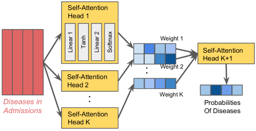
[Self-attention] [mutual-attention]

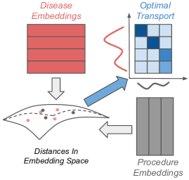
Figure 3: Illustration of the self- and mutual-attention mechanisms in our model. In (a), each self-attention head is a feed-forward neural network, whose architecture is shown in head 1.

3.3 Learning with an optimal transport-based mutual-attention mechanism

Besides the predictive loss in (2), we further design a regularizer based on the optimal-transport distance between observed diseases and procedures, achieving a mutual-attention mechanism in the training phase. As mentioned above, a disease may lead to multiple procedures and a procedure can be shared by different diseases. Therefore, for the $i$-th admission, there exists a complicated map from $\mathcal{D}_{i}$ to $\mathcal{P}_{i}^{+}$. We estimate this map explicitly via minimizing the optimal-transport distance (Villani, 2008) between $\mathcal{D}_{i}$ and $\mathcal{P}_{i}^{+}$, and the estimated map is used to regularize the learning of embeddings.

Denote the distributions of diseases and corresponding procedures in the $i$-th admission as $\bm{\mu}_{\mathcal{D}_{i}}$ and $\bm{\mu}_{\mathcal{P}_{i}^{+}}$, respectively. Here, $\bm{\mu}_{\mathcal{D}_{i}}$ is the weighted vector derived via our self-attention networks, and the $\bm{\mu}_{\mathcal{P}_{i}^{+}}$ is assumed to be a uniform distribution. As illustrated in Figure 3, given the embeddings of the diseases and the procedures, $i.e.$, $\bm{U}_{\mathcal{D}_{i}}$ and $\bm{V}_{\mathcal{P}_{i}^{+}}$, we calculate the distance matrix between them, denoted $\bm{C}_{\theta}(\mathcal{D}_{i},\mathcal{P}_{i}^{+})=[c_{dp}]\in\mathbb{R}^{|\mathcal{D}_{i}|\times|\mathcal{P}_{i}^{+}|}$. Because the probability in (1) is calculated based on the inner product between disease embedding and procedure embedding, we calculate the elements of the distance matrix based on the cosine similarity (normalized inner product) between the embeddings:

$$\begin{aligned} c_{dp}=1-\frac{\bm{u}_{d}^{\top}\bm{v}_{p}}{\|\bm{u}_{d}\|_{2}\|\bm{v}_{p}\|_{2}},~{}\forall~{}d\in\mathcal{D}_{i}~{}\mbox{and}~{}p\in\mathcal{P}_{i}^{+}.\end{aligned}$$ (5)

Based on the distance matrix, the optimal-transport distance provides a measure of the dissimilarity between $\bm{\mu}_{\mathcal{D}_{i}}$ and $\bm{\mu}_{\mathcal{P}_{i}^{+}}$, defined as

$$\begin{aligned} L_{OT}(\mathcal{D}_{i},\mathcal{P}_{i}^{+};\theta)=\sideset{}{{}_{\bm{T}\in\Pi(\bm{\mu}_{\mathcal{D}_{i}},\bm{\mu}_{\mathcal{P}_{i}^{+}})}}{\min}\langle\bm{C}_{\theta}(\mathcal{D}_{i},\mathcal{P}_{i}^{+}),\bm{T}\rangle,\end{aligned}$$ (6)

where $\Pi(\bm{\mu}_{\mathcal{D}_{i}},\bm{\mu}_{\mathcal{P}_{i}^{+}})=\{\bm{T}|\bm{T}\bm{1}_{|\mathcal{P}_{i}^{+}|}=\bm{\mu}_{\mathcal{D}_{i}},~{}\bm{T}^{\top}\bm{1}_{|\mathcal{D}_{i}|}=\bm{\mu}_{\mathcal{P}_{i}^{+}}\}$ is the set of all possible joint distributions with $\bm{\mu}_{\mathcal{D}_{i}}$ and $\bm{\mu}_{\mathcal{P}_{i}^{+}}$ as marginals; $\langle\cdot,\cdot\rangle$ represents the inner product between matrices. The optimal transport, $i.e.$, $\widehat{\bm{T}}_{i}=\arg\min_{\bm{T}\in\Pi(\bm{\mu}_{\mathcal{D}_{i}},\bm{\mu}_{\mathcal{P}_{i}^{+}})}\langle\bm{C}_{\theta}(\mathcal{D}_{i},\mathcal{P}_{i}^{+}),\bm{T}\rangle$, is the joint distribution that minimizes the distance between $\bm{\mu}_{\mathcal{D}_{i}}$ and $\bm{\mu}_{\mathcal{P}_{i}^{+}}$. A detailed introduction to the optimal-transport distance is found in Appendix A and within (Villani, 2008; Cuturi, 2013; Benamou et al., 2015).

With the help of the optimal-transport distance, we achieve a mutual-attention mechanism for embedding ICD codes: the optimal transport $\widehat{\bm{T}}_{i}$ explicitly represents the clinical relationships between $\mathcal{D}_{i}$ and $\mathcal{P}_{i}^{+}$ – if disease $d\in\mathcal{D}_{i}$ mainly yields procedure $p\in\mathcal{P}_{i}^{+}$, element $t_{dp}$ in $\widehat{\bm{T}}$ will ideally have a corresponding large value.

3.4 Proposed learning method

Given a set of admissions, $\{(\mathcal{D}_{i},\mathcal{P}_{i}^{+},\mathcal{P}_{i}^{-})\}_{i=1}^{I}$, we jointly consider the predictive loss in (2) and the optimal-transport distance in (6), and learn the proposed model by solving the following optimization problem:

$$\begin{aligned} \sideset{}{{}_{\theta}}{\min}\sideset{}{{}_{i=1}^{I}}{\sum}L_{P}(\mathcal{D}_{i},\mathcal{P}_{i}^{+},\mathcal{P}_{i}^{-};\theta)+\alpha L_{OT}(\mathcal{D}_{i},\mathcal{P}_{i}^{+};\theta){.}\end{aligned}$$ (7)

This is a nested minimization problem, because the second term involves the optimization of optimal transport. We solve this problem via alternating optimization, which involves the following two steps:

• Update optimal transport. For each admission, given current embeddings $\bm{U}_{\mathcal{D}_{i}}$ and $\bm{V}_{\mathcal{P}_{i}^{+}}$, and the estimated distribution of $\bm{\mu}_{\mathcal{D}_{i}}$, we update the optimal transport by solving (6), $i.e.$, $\widehat{\bm{T}}_{i}=\arg\sideset{}{{}_{\bm{T}\in\Pi(\bm{\mu}_{\mathcal{D}_{i}},\bm{\mu}_{\mathcal{P}_{i}^{+}})}}{\min}\langle\bm{C}_{\theta}(\mathcal{D}_{i},\mathcal{P}_{i}^{+}),\bm{T}\rangle$. This optimization problem can be solved effectively via the proximal gradient method (Xie et al., 2018), with linear convergence. The detailed introduction of the proximal gradient method is given in Appendix A.

• Update embeddings and self-attention network. Given updated optimal transport matrices $\{\widehat{\bm{T}}_{i}\}_{i=1}^{I}$, we plug them into the second term of (7), and update the ICD code embeddings and the self-attention network via mini-batch gradient descent. Specifically, we solve the following problem:

  $$\begin{aligned} \sideset{}{{}_{\theta}}{\min}\sideset{}{{}_{i\in\mathcal{B}}}{\sum}L_{P}(\mathcal{D}_{i},\mathcal{P}_{i}^{+},\mathcal{P}_{i}^{-};\theta)+\alpha\langle\bm{C}_{\theta}(\mathcal{D}_{i},\mathcal{P}_{i}^{+}),\widehat{\bm{T}}_{i}\rangle{,}\end{aligned}$$ (8)

  where $\mathcal{B}$ represents a batch of admissions.

The learning algorithm is summarized in Algorithm 1. Note that the updating of optimal transport for different admissions can be done in parallel, and the gradient of (8) can be calculated efficiently via backpropagation on graphical processing units (GPUs).

Algorithm 1 Proposed ICD code embedding method

1:  Input: Observed admissions $\{\mathcal{D}_{i},\mathcal{P}_{i}^{+}\}_{i=1}^{I}$. The dimension of embeddings $M$. The number of self-attention heads $K$. The weight of regularizer $\alpha$.

2:  Output: The parameters of proposed model $\theta$.

3:  Initialize $\theta=\{\bm{U},\bm{V},f(\cdot)\}$ randomly.

4:  while not converge do

5:     Sample a batch of admissions randomly, $i.e.$, $\{\mathcal{D}_{i},\mathcal{P}_{i}^{+}\}_{i\in\mathcal{B}}$.

6:     Sample negative procedures $\mathcal{P}_{i}^{-}$ for each admission, and get $\{\mathcal{D}_{i},\mathcal{P}_{i}^{+},\mathcal{P}_{i}^{-}\}_{i\in\mathcal{B}}$.

7:     Update optimal transport matrices:

8:     for $i\in\mathcal{B}$ do

9:        Solve (6) via proximal gradient method.

10:     end for

11:     Update model’s parameters:

12:     Solve (8) via mini-batch gradient descent.

13:  end while

4 Related Work

4.1 Embedding techniques

Embeddings have been widely used to represent and analyze real-world entities. For user-item pairs in recommendation systems, low-rank factorization models are applied to estimate user and item embeddings from their observed interactions (Herlocker et al., 1999; Rendle et al., 2009). When side information is available, such as reviews of items provided by users or the images of items, the embeddings can be further parametrized via neural networks (Kang and McAuley, 2018; Chen et al., 2018a, b). For natural language processing, word embeddings have been widely used to represent words in sentences. Typical word embedding techniques include Word2Vec (Mikolov et al., 2013) and GloVe (Pennington et al., 2014), which maximize the coherency of the words and their contexts in sentences. Following the same strategy, many node embedding methods have been proposed to represent nodes in graphs, $e.g.$, DeepWalk (Perozzi et al., 2014), LINE (Tang et al., 2015), and Node2Vec (Grover and Leskovec, 2016). Most of these embedding methods employ the same framework – first generate sequential observations through random walks in the graph, and then apply word embeddings by maximizing the coherency of adjacent nodes on the random walks. Focusing on clinical data analysis, embedding techniques have been applied to many tasks, like ICD code assignment (Shi et al., 2017; Baumel et al., 2017; Mullenbach et al., 2018; Huang et al., 2018), clinical data clustering, and treatment prediction (Bajor et al., 2018; Harutyunyan et al., 2017; Choi et al., 2016a). Recently, the work in (Xu et al., 2018, 2019) makes efforts to learn ICD code embeddings directly through admission records based on optimal transport-based methods. However, the methods don’t scale well, and therefore it is hard to apply in practical systems.

4.2 Attention models

Attention models have proven useful for many machine learning tasks. Such models are typically applied to a set or sequence of vectors, and the associated weights on the vectors characterize their importance for a given task (Vinyals et al., 2015). The weights highlight the important parts of the sequence of vectors, and effectively provide an adaptive pooling strategy to obtain a global representation of all observations (Lin et al., 2017). A successful example of attention models is its application to natural language processing (NLP) tasks, like question-answering and document comprehension (Devlin et al., 2018; Choi et al., 2017b) – the attention model has been core to advanced NLP modules like the “transformer” (Vaswani et al., 2017). Leading language models like GPT (Radford et al., 2018) and BERT (Devlin et al., 2018) also rely on various attention mechanisms. Besides NLP, attention models have recently been applied to other tasks, including recommendation systems (Kang and McAuley, 2018), imitation learning (Kool and Welling, 2018), and multi-instance learning (Ilse et al., 2018). Attention models are also applicable for healthcare, a, $e.g.$, ECG rhythm classification (Goodfellow et al., 2018), admission prediction (Choi et al., 2016b), and heart failure prediction (Choi et al., 2017a).

4.3 Optimal transport-based learning

Learning based on the optimal-transport distance has recently attracted much attention, such as in distribution estimation (Boissard et al., 2015) and clustering (Ye et al., 2017). It can also be used as a loss function when learning deep generative models (Courty et al., 2017; Arjovsky et al., 2017). The main bottleneck of the application of optimal-transport distance is its high computational complexity. This problem has been eased greatly by the Sinkhorn-Knopp algorithm (Sinkhorn and Knopp, 1967). Specifically, by adding an entropy regularizer (Cuturi, 2013), the optimal-transport distance can be approximated via iterative Bregman projection (Benamou et al., 2015). The algorithm achieves near-linear-time complexity (Altschuler et al., 2017), and its convergence and stability can be further improved via the inexact proximal point method (Xie et al., 2018). However, the application of optimal transport to problems in healthcare has not been widely investigated.

5 Experiments

5.1 Comparisons on procedure recommendation

To demonstrate the effectiveness of the proposed embedding method, we test it on the three datasets introduced in Section 2 and compare it with its variants and existing embedding methods. Specifically, we denote our Embedding method with Self- and Mutual-Attention mechanisms as E+SA+MA. Its variants include: 1) setting the fusion function to a max-pooling function, and learning without optimal transport-based mutual-attention regularizer ($i.e.$, E+Pooling); 2) using the proposed self-attention network as the fusion function, but learning without the mutual-attention regularizer ($i.e.$, E+SA); and 3) using max-pooling as the fusion function but considering the mutual-attention regularizer ($i.e.$, E+MA). These variants provide understanding of the significance of the self- and mutual-attention mechanisms. The key hyperparameters of the proposed method include the dimension of the embedding vector $M$, the weight of the mutual-attention regularizer $\alpha$ and the number of heads in the self-attention network $K$. In all models we set $M=200$, $\alpha=0.1$, and $K=8$. The robustness of our method to these hyperparameters is analyzed in Section 5.2. All the methods learn ICD code embeddings via Adam (Kingma and Ba, 2014), setting the learning rate to $0.001$, batch size as $300$, and the number of epochs as $25$.

We also consider the following methods as baselines: 1) the Word2Vec method (Mikolov et al., 2013), which enumerates all possible disease-procedure pairs in each admission, and learns the ICD code embeddings to maximize the log-likelihood of the pairs; 2) the classical Bayesian personalized ranking method (BPR) (Rendle et al., 2009), which maximizes the coherency between the averaged disease embedding and the procedure embeddings in each admission; 3) the distilled Wasserstein method (DWL) (Xu et al., 2018), that learns the ICD code embeddings via a hierarchical optimal transport-based method; and 4) the Gromov-Wasserstein learning method (GWL) (Xu et al., 2019), that learns the ICD code embeddings with structural regularization on the embeddings within the domain of diseases and that of procedures. Similar to our method, these baselines also learn ICD code embeddings with dimension $M=200$.

Table 1: Comparison for various methods on recommendation results

Dataset	Method	Top-1 (%)			Top-3 (%)			Top-5 (%)			Top-10 (%)
		R	P	F1	R	P	F1	R	P	F1	R	P	F1
	Word2Vec	19.5	47.8	24.7	35.4	34.9	30.8	47.1	29.6	32.0	62.3	21.1	28.5
28,315	DWL	19.7	48.2	25.0	35.9	35.2	31.3	47.5	30.3	32.4	63.0	20.9	28.7
Admissions	GWL	13.1	44.9	18.0	19.2	25.2	18.8	23.9	21.6	19.5	40.1	20.0	24.3
247	BPR	23.5	57.6	29.8	44.8	43.5	38.7	56.8	35.7	38.8	73.1	24.8	33.6
Diseases	E+Pooling	24.5	58.5	30.9	46.2	44.0	39.6	58.0	35.7	39.1	74.5	25.1	34.0
75	E+SA	24.4	58.4	30.8	45.8	43.7	39.2	57.2	35.7	38.9	73.6	24.9	33.7
Procedures	E+MA	23.7	57.4	30.0	45.2	43.2	38.8	57.4	35.6	38.8	74.2	25.0	33.8
	E+SA+MA	24.8	59.7	31.3	46.4	44.1	39.7	58.7	36.3	39.7	74.9	25.3	34.2
	Word2Vec	7.8	27.6	10.9	27.7	30.5	25.1	38.3	26.9	27.7	52.8	20.1	26.1
30,535	DWL	8.0	27.5	11.1	27.9	30.8	25.2	39.5	27.0	27.9	53.9	20.9	27.4
Admissions	GWL	9.2	36.9	13.2	11.8	15.9	11.6	12.7	10.9	10.0	15.8	7.8	8.9
874	BPR	10.2	35.8	14.9	38.6	40.2	34.3	49.3	33.3	34.9	65.2	23.8	31.4
Diseases	E+Pooling	10.1	35.4	14.3	38.0	39.7	33.9	50.0	33.6	35.3	65.6	24.1	31.7
258	E+SA	18.2	50.0	23.6	36.6	39.1	33.0	48.7	33.1	34.6	66.0	24.1	31.8
Procedures	E+MA	12.4	32.4	15.7	38.7	39.3	34.0	50.9	33.9	35.7	67.6	24.7	32.5
	E+SA+MA	20.3	53.1	26.1	40.7	42.3	36.2	53.0	35.4	37.2	68.9	25.1	33.1
	Word2Vec	5.3	22.9	8.7	14.6	21.1	15.3	24.8	21.0	20.1	41.1	17.7	22.2
31,213	DWL	5.6	23.0	9.0	14.9	21.3	15.6	24.8	21.4	20.5	42.0	18.2	23.0
Admissions	GWL	5.5	19.0	7.5	5.6	6.6	5.1	5.7	4.2	4.1	6.0	2.3	2.9
2,765	BPR	7.3	26.7	10.2	23.0	27.1	21.2	38.4	27.6	27.9	56.6	21.7	28.0
Diseases	E+Pooling	7.4	27.3	10.4	16.5	23.3	17.1	38.7	27.3	27.8	58.3	22.0	28.6
819	E+SA	8.0	28.2	11.1	20.0	26.0	19.7	36.5	26.5	26.6	56.6	21.7	28.0
Procedures	E+MA	6.9	25.7	9.7	18.5	22.7	17.5	33.2	23.4	23.8	56.5	21.5	27.8
	E+SA+MA	8.5	27.9	11.4	23.1	27.2	21.4	39.1	27.9	28.4	60.0	22.8	29.6

For each dataset, we use 80% of the admissions for training and 20% for testing. In the testing phase, we evaluate each embedding method for the task of recommending procedures according to diagnosed diseases. Similar to other works of recommendation systems, we evaluate the performance of each method in the testing phase via top-$L$ precision, recall, and F1-score. For the $i$-th testing admission, $i\in\{1,...,I\}$, each method recommends a set of procedures with length $L$, denoted $\widehat{\mathcal{P}}_{i}^{+}$. Given the ground-truth set $\mathcal{P}_{i}^{+}$, we calculate the top-$L$ precision, recall and F1-score as follows:

$$\begin{aligned} P\text{=}\sum_{i=1}^{I}P_{i}\text{=}\sum_{i=1}^{I}\frac{|\widehat{\mathcal{P}}_{i}^{+}\cap\mathcal{P}_{i}^{+}|}{|\widehat{\mathcal{P}}_{i}^{+}|}\times 100\%,~{}R\text{=}\sum_{i=1}^{I}R_{i}\text{=}\sum_{i=1}^{I}\frac{|\widehat{\mathcal{P}}_{i}^{+}\cap\mathcal{P}_{i}^{+}|}{|\mathcal{P}_{i}^{+}|}\times 100\%,~{}F1\text{=}\sum_{i=1}^{I}\frac{2P_{i}R_{i}}{P_{i}+R_{i}}.\end{aligned}$$

For each method, the embedding model is learned on the training admissions with 10-fold cross validation. In particular, the model is learned on 9-fold of training admission, validated on the remaining fold, and tested on the testing admission. The averaged top-$L$ measurements of each model, with $L=1,~{}3,~{}5,~{}10$, are recorded in Table 1. We find that the proposed E+SA+MA method outperforms the alternatives consistently across different datasets and for all measurements. Specifically, among existing methods, only BPR is comparable to that of E+Pooling (the simplest variant of our method). Considering self-attention or mutual-attention mechanism indeed boosts the recommendation result in most situations, as shown in the rows of E+SA and E+MA. Accordingly, combining these two mechanisms jointly ($i.e.$, our E+SA+MA) can achieve the best performance.

5.2 Robustness to hyperparameters

As discussed above, the dimension $M$ of the embedding vectors, the weight of mutual-attention regularizer $\alpha$, and the number of self-attention heads $K$ are important for our method, having significant influence on the recommendation results. Figure 4 illustrates the influence of these hyperparameters on the F1-scores derived by our method on the small dataset. In Figure 4, we find that when the dimension of embedding falls in the range from $100$ to $300$, the performance of our method is relatively stable. Setting $M=200$ achieves slightly better performance. When the dimension is too small, $e.g.$, $M=20$ or $50$, the embeddings are not representative enough, which leads to under-fitting. In Figure 4 we set $\alpha=0.01,0.1,1,10$. The proposed method obtains comparable F1-scores when $\alpha$ falls in the range $0.1$ to $1$. When $\alpha$ is too large, $e.g.$, $\alpha=10$, the proposed regularizer is too strong and becomes dominant in the loss function. As a result, the model suffers from serious model misspecification and the recommendation results degrade accordingly. In Figure 4, we set $K=1,4,8,12,16$. When $K=1$, the self-attention network only contains one attention layer with one head. With the increase of $K$, the number of parameters in the self-attention network becomes larger and the model becomes more representative. When $K=8$, the best performance is achieved. If we further increase $K$, our model will have too many parameters and suffer from over-fitting. The illustrations on the medium and the large datasets are similar to Figure 4. Based on the analysis above, we empirically set $M=200$, $\alpha=0.1$ and $K=8$.

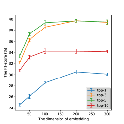
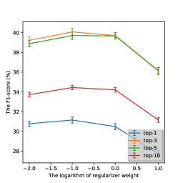
[F1 v.s. dimension $M$, with $\alpha=0.1$, $K=8$] [F1 v.s. weight $\alpha$, with $M=200$, $K=8$] [F1 v.s. head number $K$, with $M=200$, $\alpha=0.1$]

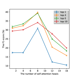
Figure 4: Illustrations of the robustness of our method to its hyperparameters, including the dimension of embedding $M$, the weight of the mutual-attention regularizer $\alpha$ and the number of heads in the self-attention network $K$.

5.3 Interpretability

The embeddings we learn are found to have good interpretability. Specifically, given a set of diseases, our self-attention network estimates the significance of the diseases. Given predicted procedures, we can further calculate the optimal transport between the observed diseases and the predicted procedures explicitly via the mutual-attention regularizer. Figure 5 shows typical procedure recommendation results. Each row corresponds to the result of an admission. For each admission, we observe some diagnosed diseases and recommended top-5 procedures. Given the diagnosed diseases, their significance ($i.e.$, $\bm{\mu}_{\mathcal{D}_{i}}$) and their optimal transport ($i.e.$, $\widehat{\bm{T}}_{i}$) to the recommended procedures are shown. We find that the significance reflects the seriousness of diseases: in Figure 5, the urgent disease “Cardiac arrest” is assigned with the highest significance; in Figure 5, dangerous diseases like “Acute kidney failure” are assigned with high significance. Additionally, the optimal transport estimates reasonable clinical relationships between diseases and procedures. For example, in Figure 5, we find that the disease “End stage renal disease” will transport to its regular procedure “Hemodialysis”, and the disease “Cardiac arrest” will transport to the suitable procedure “Cardiopulmonary resuscitation”. In Figure 5, the disease “Acute and chronic respiratory failure” may yield procedure “Continuous invasive mechanical ventilation”. In Figure 5, the disease “Other pulmonary insufficiency” may lead to “Insertion of endotracheal tube”. More examples can be found in Appendix B.

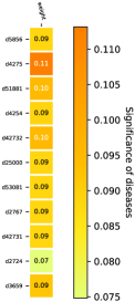
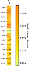
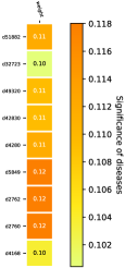
[Descriptions of ICD codes] d5856 End stage renal disease d4275 Cardiac arrest d51881 Acute respiratory failure d4254 Other primary cardiomyopathies d42732 Atrial flutter d25000 Diabetes mellitus without complication, type II d53081 Esophageal reflux d2767 Hyperpotassemia d42731 Atrial fibrillation d2724 Other and unspecified hyperlipidemia d3659 Unspecified glaucoma p3893 Venous catheterization, not elsewhere classified p9960 Cardiopulmonary resuscitation, not otherwise specified p9671 Continuous invasive mechanical ventilation p9604 Insertion of endotracheal tube p3995 Hemodialysis [$\bm{\mu}_{\mathcal{D}_{i}}$] [$\widehat{\bm{T}}_{i}$]
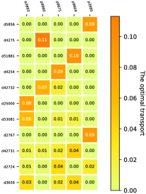
[Descriptions of ICD codes] d0389 Unspecified septicemia d78552 Septic shock d43411 Cerebral embolism with cerebral infarction d51884 Acute and chronic respiratory failure d41071 Subendocardial infarction, initial episode of care d5845 Acute kidney failure with lesion of tubular necrosis d4280 Congestive heart failure, unspecified d5990 Urinary tract infection, site not specified dV5867 Long-term (current) use of insulin d2948 Other persistent mental disorders d4019 Unspecified essential hypertension dV4501 Cardiac pacemaker d99592 Severe sepsis p17 Infusion of vasopressor agent p9604 Insertion of endotracheal tube p9672 Continuous invasive mechanical ventilation p966 Enteral infusion of concentrated nutritional substances p3893 Venous catheterization, not elsewhere classified [$\bm{\mu}_{\mathcal{D}_{i}}$] [$\widehat{\bm{T}}_{i}$]
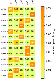
[Descriptions of ICD codes] d51882 Other pulmonary insufficiency, not elsewhere classified d32723 Obstructive sleep apnea (adult)(pediatric) d49320 Chronic obstructive asthma, unspecified d42830 Diastolic heart failure, unspecified d4280 Congestive heart failure, unspecified d5849 Acute kidney failure, unspecified d2762 Acidosis d2760 Hyperosmolality and/or hypernatremia d4168 Other chronic pulmonary heart diseases p3891 Arterial catheterization p9671 Continuous invasive mechanical ventilation p9604 Insertion of endotracheal tube p3893 Venous catheterization, not elsewhere classified p9390 Non-invasive mechanical ventilation [$\bm{\mu}_{\mathcal{D}_{i}}$] [$\widehat{\bm{T}}_{i}$]

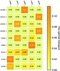
Figure 5: Typical examples showing the interpretability of our method. For each row, the descriptions of diagnosed diseases and recommended procedures, the estimated significance of the diseases, and the optimal transport between the diseases and the procedures are shown from left to right.

6 Conclusions and Future Work

A novel embedding method has been proposed for ICD codes, which has self- and mutual-attention mechanisms and outperforms existing embedding methods in procedure recommendation. The self-attention network in the proposed method achieves an adaptive fusion strategy of disease embeddings, which estimates the significance of various diseases in different admissions. An optimal transport-based mutual-attention regularizer is considered in the training phase of our model, estimating the clinical relationship between the diseases and the procedures appearing in the same admissions. These two mechanisms enhance the interpretability of the learned embeddings and improve the recommendation accuracy. In the future, we plan to design more-effective attention mechanisms and further improve the representation power of embeddings. Additionally, beyond the MIMIC-III, we will explore the performance of our method in real-world large-scale data.

Appendix A Proximal Gradient Method for Optimal Transport

Mathematically, the optimal-transport distance can be defined as follows (Villani, 2008):

Definition A.1.

Let $(\Omega,D)$ be an arbitrary space with metric $D$ and $P(\Omega)$ the set of Borel probability measures on $\Omega$. For probability measures $u$ and $v$ in $P(\Omega)$, their optimal-transport distance is

$$\begin{aligned} W(u,v):=\sideset{}{{}_{\pi\in\Pi(u,v)}}{\inf}\int_{\Omega\times\Omega}D(x,y)d\pi(x,y),\end{aligned}$$ (9)

where $\Pi(u,v)$ is the set of all probability measures on $\Omega\times\Omega$ with $u$ and $v$ as marginals.

When the metric $D$ is Euclidean, the optimal transport distace corresponds to well-known Wasserstein distance (Villani, 2008; Cuturi, 2013). When $D$ is not a valid metric, the optimal-transport distance corresponds to the classcial Monge–Kantorovich transportation problem.

For the discrete case in our work, given a set of diseases $\mathcal{D}_{i}$, a set of procedures $\mathcal{P}_{i}^{+}$, and their distributions $\bm{\mu}_{\mathcal{D}_{i}}\in\Sigma^{|\mathcal{D}_{i}|}$ and $\bm{\mu}_{\mathcal{P}_{i}^{+}}\in\Sigma^{|\mathcal{P}_{i}^{+}|}$, the definition in (9) can be reformulated as (6), where the cost matrix $\bm{C}(\mathcal{D}_{i},\mathcal{P}_{i}^{+})$ is calculated via (5).

Algorithm 2 Proximal gradient method for optimal transport

1:  Input: Cost matrix $\bm{C}_{\theta}(\mathcal{D}_{i},\mathcal{P}_{i}^{+})$, the distributions of diseases and procedures $\bm{\mu}_{\mathcal{D}_{i}}$ and $\bm{\mu}_{\mathcal{P}_{i}^{+}}$, the weight of proximal term $\beta=0.5$.

2:  Output: Optimal transport $\bm{T}$

3:  Calculate $\bm{G}=\exp(-\frac{\bm{C}_{\theta}(\mathcal{D}_{i},\mathcal{P}_{i}^{+})}{\beta})$, and initialize $\bm{a}=\bm{1}_{|\mathcal{D}_{i}|}$, $\bm{T}=\bm{\mu}_{\mathcal{D}_{i}}\bm{\mu}_{\mathcal{P}_{i}^{+}}^{\top}$

4:  while not converge do

5:     $\bm{K}=\bm{G}\odot\bm{T}$

6:     while not converge do

7:        Sinkhorn-Knopp Iteration: $\bm{b}=\frac{\bm{\mu}_{\mathcal{P}_{i}^{+}}}{\bm{K}^{\top}\bm{a}}$, and then $\bm{a}=\frac{\bm{\mu}_{\mathcal{D}_{i}}}{\bm{K}\bm{b}}$.

8:     end while

9:     $\bm{T}=(\bm{a}\bm{b}^{\top})\odot\bm{K}$

10:  end while

We solve (6) via the proximal gradient method proposed in (Xie et al., 2018). In particular, this method solves (6) iteratively. In the $j$-th iteration, a proximal term is added to original problem as

$$\begin{aligned} \bm{T}^{(j)}=\arg\sideset{}{{}_{\bm{T}\in\Pi(\bm{\mu}_{\mathcal{D}_{i}},\bm{\mu}_{\mathcal{P}_{i}^{+}})}}{\min}\langle\bm{C}_{\theta}(\mathcal{D}_{i},\mathcal{P}_{i}^{+}),\bm{T}\rangle+\beta\mbox{KL}(\bm{T}\lVert\bm{T}^{(j-1)}),\end{aligned}$$ (10)

where $\bm{T}^{(j-1)}$ is the optimal transport learned in previous iteration, and the proximal term is $\mbox{KL}(\bm{T}\lVert\bm{T}^{(j-1)})=\sum_{d,p}t_{dp}\log\frac{t_{dp}}{t_{dp}^{(j-1)}}$.

The optimization problem in (10) can be rewritten as

$$\begin{aligned} \bm{T}^{(j)}=\arg\sideset{}{{}_{\bm{T}\in\Pi(\bm{\mu}_{\mathcal{D}_{i}},\bm{\mu}_{\mathcal{P}_{i}^{+}})}}{\min}\langle\bm{C}_{\theta}(\mathcal{D}_{i},\mathcal{P}_{i}^{+})-\beta\log\bm{T}^{(j-1)},\bm{T}\rangle+\beta\langle\log\bm{T},\bm{T}\rangle,\end{aligned}$$ (11)

where the second term is the entropy regularizer used in (Cuturi, 2013). Accordingly, Sinkhorn-Knopp iteration can be applied to solve (11) effectively. In summary, the proposed proximal gradient method is shown in Algorithm 2. This method has linear convergence and has good numerical stability. More detailed analysis can be found in (Xie et al., 2018; Xu et al., 2019).

Appendix B Typical Examples of Learning Results

In Figures 6 and 7, we visualize the learning results of 6 admissions. For each admission, the significance of its diagnosed diseases ($i.e.$, $\bm{\mu}_{\mathcal{D}_{i}}$) and the optimal transport between the diseases and the recommended top-5 procedures ($i.e.$, $\widehat{\bm{T}}_{i}$) are shown. We can find that the significance learned by our method often indicates the main diseases or the most serious diseases in the admissions. The nonzero elements in the optimal transports often correspond to the pairs of the diseases and their related procedures.

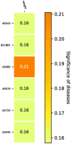
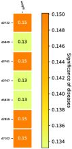
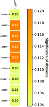
[Descriptions of ICD codes] d0543 Herpetic meningoencephalitis d51881 Acute respiratory failure d3485 Cerebral edema d4019 Unspecified essential hypertension d2720 Pure hypercholesterolemia d4240 Mitral valve disorders p331 Incision of lung p9671 Continuous invasive mechanical ventilation p9604 Insertion of endotracheal tube p966 Enteral infusion of concentrated nutritional substances p3893 Venous catheterization, not elsewhere classified [$\bm{\mu}_{\mathcal{D}_{i}}$] [$\widehat{\bm{T}}_{i}$]
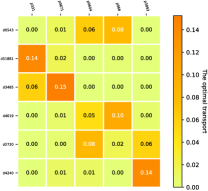
[Descriptions of ICD codes] d2732 Other paraproteinemias d5849 Acute kidney failure, unspecified d2761 Hyposmolality and/or hyponatremia d2767 Hyperpotassemia d5839 Nephritis and nephropathy d2859 Anemia, unspecified d7102 Sicca syndrome p9971 Therapeutic plasmapheresis p3893 Venous catheterization, not elsewhere classified p5523 Closed [percutaneous] [needle] biopsy of kidney p3895 Venous catheterization for renal dialysis p3995 Hemodialysis [$\bm{\mu}_{\mathcal{D}_{i}}$] [$\widehat{\bm{T}}_{i}$]
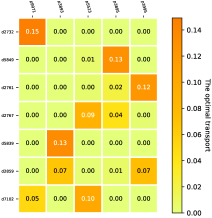
[Descriptions of ICD codes] d4240 Mitral valve disorders d5859 Chronic kidney disease, unspecified d42731 Atrial fibrillation d2449 Unspecified acquired hypothyroidism d4019 Unspecified essential hypertension d2720 Pure hypercholesterolemia dV5861 Long-term (current) use of anticoagulants d2859 Anemia, unspecified d2749 Gout, unspecified p3733 Excision or destruction of other lesion or tissue of heart p8872 Diagnostic ultrasound of heart p3523 Open and replacement of mitral valve with tissue graft p9904 Transfusion of packed cells p3961 Extracorporeal circulation auxiliary to open heart surgery [$\bm{\mu}_{\mathcal{D}_{i}}$] [$\widehat{\bm{T}}_{i}$]

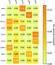
Figure 6: Typical examples showing the interpretability of our method. For each row, the descriptions of diagnosed diseases and recommended procedures, the estimated significance of the diseases, and the optimal transport between the diseases and the procedures are shown from left to right.

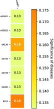
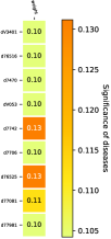
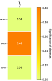
[Descriptions of ICD codes] d41401 Coronary atherosclerosis of native coronary artery d42822 Chronic systolic heart failure d4139 Other and unspecified angina pectoris d2720 Pure hypercholesterolemia d2749 Gout, unspecified d4280 Congestive heart failure, unspecified d412 Old myocardial infarction p3612 (Aorto)coronary bypass of two coronary arteries p8856 Coronary arteriography using two catheters p3722 Left heart cardiac catheterization p3961 Circulation auxiliary to open heart surgery p3615 Single internal mammary-coronary artery bypass [$\bm{\mu}_{\mathcal{D}_{i}}$] [$\widehat{\bm{T}}_{i}$]
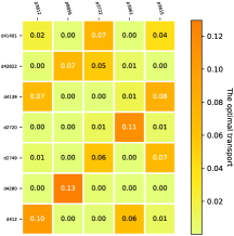
[Descriptions of ICD codes] dV3401 Other multiple birth (three or more), mates all liveborn d76516 Other preterm infants, 1,500-1,749 grams d7470 Patent ductus arteriosus dV053 Need for prophylactic vaccination against viral hepatitis d7742 Neonatal jaundice associated with preterm delivery d7706 Transitory tachypnea of newborn d76525 29-30 completed weeks of gestation d77081 Primary apnea of newborn d77981 Neonatal bradycardia p9604 Insertion of endotracheal tube p9390 Non-invasive mechanical ventilation p966 Enteral infusion of concentrated nutritional substances p9983 Other phototherapy p9955 Prophylactic administration of vaccine [$\bm{\mu}_{\mathcal{D}_{i}}$] [$\widehat{\bm{T}}_{i}$]
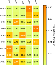
[Descriptions of ICD codes] d41401 Coronary atherosclerosis of native coronary artery d4019 Unspecified essential hypertension d2720 Pure hypercholesterolemia p3612 (Aorto)coronary bypass of two coronary arteries p8856 Coronary arteriography using two catheters p3722 Left heart cardiac catheterization p3961 Circulation auxiliary to open heart surgery p3615 Single internal mammary-coronary artery bypass [$\bm{\mu}_{\mathcal{D}_{i}}$] [$\widehat{\bm{T}}_{i}$]

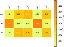
Figure 7: Typical examples showing the interpretability of our method. For each row, the descriptions of diagnosed diseases and recommended procedures, the estimated significance of the diseases, and the optimal transport between the diseases and the procedures are shown from left to right.

References

- Altschuler et al. (2017) Jason Altschuler, Jonathan Weed, and Philippe Rigollet. Near-linear time approximation algorithms for optimal transport via Sinkhorn iteration. arXiv preprint arXiv:1705.09634, 2017.
- Arjovsky et al. (2017) Martin Arjovsky, Soumith Chintala, and Léon Bottou. Wasserstein generative adversarial networks. In ICML, pages 214–223, 2017.
- Bajor et al. (2018) Jacek M Bajor, Diego A Mesa, Travis J Osterman, and Thomas A Lasko. Embedding complexity in the data representation instead of in the model: A case study using heterogeneous medical data. arXiv preprint arXiv:1802.04233, 2018.
- Baumel et al. (2017) Tal Baumel, Jumana Nassour-Kassis, Michael Elhadad, and Noemie Elhadad. Multi-label classification of patient notes a case study on ICD code assignment. arXiv preprint arXiv:1709.09587, 2017.
- Benamou et al. (2015) Jean-David Benamou, Guillaume Carlier, Marco Cuturi, Luca Nenna, and Gabriel Peyré. Iterative Bregman projections for regularized transportation problems. SIAM Journal on Scientific Computing, 37(2):A1111–A1138, 2015.
- Boissard et al. (2015) Emmanuel Boissard, Thibaut Le Gouic, Jean-Michel Loubes, et al. Distribution’s template estimate with wasserstein metrics. Bernoulli, 21(2):740–759, 2015.
- Chen et al. (2018a) Xu Chen, Hongteng Xu, Yongfeng Zhang, Jiaxi Tang, Yixin Cao, Zheng Qin, and Hongyuan Zha. Sequential recommendation with user memory networks. In WSDM, pages 108–116. ACM, 2018a.
- Chen et al. (2018b) Xu Chen, Yongfeng Zhang, Hongteng Xu, Zheng Qin, and Hongyuan Zha. Adversarial distillation for efficient recommendation with external knowledge. ACM Transactions on Information Systems (TOIS), 37(1):12, 2018b.
- Choi et al. (2016a) Edward Choi, Mohammad Taha Bahadori, Elizabeth Searles, Catherine Coffey, Michael Thompson, James Bost, Javier Tejedor-Sojo, and Jimeng Sun. Multi-layer representation learning for medical concepts. In KDD, 2016a.
- Choi et al. (2016b) Edward Choi, Mohammad Taha Bahadori, Jimeng Sun, Joshua Kulas, Andy Schuetz, and Walter Stewart. Retain: An interpretable predictive model for healthcare using reverse time attention mechanism. In NIPS, pages 3504–3512, 2016b.
- Choi et al. (2017a) Edward Choi, Mohammad Taha Bahadori, Le Song, Walter F Stewart, and Jimeng Sun. Gram: graph-based attention model for healthcare representation learning. In KDD, pages 787–795. ACM, 2017a.
- Choi et al. (2017b) Eunsol Choi, Daniel Hewlett, Jakob Uszkoreit, Illia Polosukhin, Alexandre Lacoste, and Jonathan Berant. Coarse-to-fine question answering for long documents. In ACL, volume 1, pages 209–220, 2017b.
- Courty et al. (2017) Nicolas Courty, Rémi Flamary, and Mélanie Ducoffe. Learning Wasserstein embeddings. arXiv preprint arXiv:1710.07457, 2017.
- Cuturi (2013) Marco Cuturi. Sinkhorn distances: Lightspeed computation of optimal transport. In NIPS, pages 2292–2300, 2013.
- Devlin et al. (2018) Jacob Devlin, Ming-Wei Chang, Kenton Lee, and Kristina Toutanova. Bert: Pre-training of deep bidirectional transformers for language understanding. arXiv preprint arXiv:1810.04805, 2018.
- Goodfellow et al. (2018) Sebastian D Goodfellow, Andrew Goodwin, Robert Greer, Peter C Laussen, Mjaye Mazwi, and Danny Eytan. Towards understanding ecg rhythm classification using convolutional neural networks and attention mappings. In Machine Learning for Healthcare Conference, pages 83–101, 2018.
- Grover and Leskovec (2016) Aditya Grover and Jure Leskovec. node2vec: Scalable feature learning for networks. In KDD, pages 855–864, 2016.
- Harutyunyan et al. (2017) Hrayr Harutyunyan, Hrant Khachatrian, David C Kale, and Aram Galstyan. Multitask learning and benchmarking with clinical time series data. arXiv preprint arXiv:1703.07771, 2017.
- Herlocker et al. (1999) Jonathan L Herlocker, Joseph A Konstan, Al Borchers, and John Riedl. An algorithmic framework for performing collaborative filtering. In SIGIR, pages 230–237. Association for Computing Machinery, Inc, 1999.
- Huang et al. (2018) Jinmiao Huang, Cesar Osorio, and Luke Wicent Sy. An empirical evaluation of deep learning for ICD-9 code assignment using MIMIC-III clinical notes. arXiv preprint arXiv:1802.02311, 2018.
- Ilse et al. (2018) Maximilian Ilse, Jakub M Tomczak, and Max Welling. Attention-based deep multiple instance learning. arXiv preprint arXiv:1802.04712, 2018.
- Johnson et al. (2016) Alistair EW Johnson, Tom J Pollard, Lu Shen, H Lehman Li-wei, Mengling Feng, Mohammad Ghassemi, Benjamin Moody, Peter Szolovits, Leo Anthony Celi, and Roger G Mark. MIMIC-III, a freely accessible critical care database. Scientific data, 3:160035, 2016.
- Kang and McAuley (2018) Wang-Cheng Kang and Julian McAuley. Self-attentive sequential recommendation. arXiv preprint arXiv:1808.09781, 2018.
- Kingma and Ba (2014) Diederik P Kingma and Jimmy Ba. Adam: A method for stochastic optimization. arXiv preprint arXiv:1412.6980, 2014.
- Kool and Welling (2018) WWM Kool and M Welling. Attention solves your tsp. arXiv preprint arXiv:1803.08475, 2018.
- Lin et al. (2017) Zhouhan Lin, Minwei Feng, Cicero Nogueira dos Santos, Mo Yu, Bing Xiang, Bowen Zhou, and Yoshua Bengio. A structured self-attentive sentence embedding. arXiv preprint arXiv:1703.03130, 2017.
- Mahmood et al. (2018) Rafid Mahmood, Aaron Babier, Andrea McNiven, Adam Diamant, and Timothy CY Chan. Automated treatment planning in radiation therapy using generative adversarial networks. In Machine Learning for Healthcare Conference, pages 484–499, 2018.
- Mikolov et al. (2013) Tomas Mikolov, Kai Chen, Greg Corrado, and Jeffrey Dean. Efficient estimation of word representations in vector space. arXiv preprint arXiv:1301.3781, 2013.
- Mullenbach et al. (2018) James Mullenbach, Sarah Wiegreffe, Jon Duke, Jimeng Sun, and Jacob Eisenstein. Explainable prediction of medical codes from clinical text. arXiv preprint arXiv:1802.05695, 2018.
- Pennington et al. (2014) Jeffrey Pennington, Richard Socher, and Christopher Manning. Glove: Global vectors for word representation. In EMNLP, pages 1532–1543, 2014.
- Perozzi et al. (2014) Bryan Perozzi, Rami Al-Rfou, and Steven Skiena. Deepwalk: Online learning of social representations. In KDD, pages 701–710, 2014.
- Radford et al. (2018) Alec Radford, Karthik Narasimhan, Tim Salimans, and Ilya Sutskever. Improving language understanding by generative pre-training. https://blog.openai.com/language-unsupervised/, 2018.
- Rendle et al. (2009) Steffen Rendle, Christoph Freudenthaler, Zeno Gantner, and Lars Schmidt-Thieme. Bpr: Bayesian personalized ranking from implicit feedback. In Proceedings of the twenty-fifth conference on uncertainty in artificial intelligence, pages 452–461. AUAI Press, 2009.
- Shi et al. (2017) Haoran Shi, Pengtao Xie, Zhiting Hu, Ming Zhang, and Eric P Xing. Towards automated ICD coding using deep learning. arXiv preprint arXiv:1711.04075, 2017.
- Sinkhorn and Knopp (1967) Richard Sinkhorn and Paul Knopp. Concerning nonnegative matrices and doubly stochastic matrices. Pacific Journal of Mathematics, 21(2):343–348, 1967.
- Tang et al. (2015) Jian Tang, Meng Qu, Mingzhe Wang, Ming Zhang, Jun Yan, and Qiaozhu Mei. Line: Large-scale information network embedding. In WWW, pages 1067–1077, 2015.
- Vaswani et al. (2017) Ashish Vaswani, Noam Shazeer, Niki Parmar, Jakob Uszkoreit, Llion Jones, Aidan N Gomez, Łukasz Kaiser, and Illia Polosukhin. Attention is all you need. In NIPS, pages 5998–6008, 2017.
- Villani (2008) Cédric Villani. Optimal transport: Old and new, volume 338. Springer Science & Business Media, 2008.
- Vinyals et al. (2015) Oriol Vinyals, Meire Fortunato, and Navdeep Jaitly. Pointer networks. In NIPS, pages 2692–2700, 2015.
- Xie et al. (2018) Yujia Xie, Xiangfeng Wang, Ruijia Wang, and Hongyuan Zha. A fast proximal point method for computing wasserstein distance. arXiv preprint arXiv:1802.04307, 2018.
- Xu et al. (2018) Hongteng Xu, Wenlin Wang, Wei Liu, and Lawrence Carin. Distilled wasserstein learning for word embedding and topic modeling. In NIPS, pages 1723–1732, 2018.
- Xu et al. (2019) Hongteng Xu, Dixin Luo, Hongyuan Zha, and Lawrence Carin. Gromov-wasserstein learning for graph matching and node embedding. arXiv preprint arXiv:1901.06003, 2019.
- Ye et al. (2017) Jianbo Ye, Panruo Wu, James Z Wang, and Jia Li. Fast discrete distribution clustering using Wasserstein barycenter with sparse support. IEEE Transactions on Signal Processing, 65(9):2317–2332, 2017.