Utilizing Edge Features in Graph Neural Networks via Variational Information Maximization

Abstract

Graph Neural Networks (GNNs) achieve an impressive performance on structured graphs by recursively updating the representation vector of each node based on its neighbors, during which parameterized transformation matrices should be learned for the node feature updating. However, existing propagation schemes are far from being optimal since they do not fully utilize the relational information between nodes. We propose the information maximizing graph neural networks (IGNN), which maximizes the mutual information between edge states and transform parameters. We reformulate the mutual information as a differentiable objective via a variational approach. We compare our model against several recent variants of GNNs and show that our model achieves the state-of-the-art performance on multiple tasks including quantum chemistry regression on QM9 dataset, generalization capability from QM9 to larger molecular graphs, and prediction of molecular bioactivities relevant for drug discovery. The IGNN model is based on an elegant and fundamental idea in information theory as explained in the main text, and it could be easily generalized beyond the contexts of molecular graphs considered in this work. To encourage more future work in this area, all datasets and codes used in this paper will be released for public access.

1 Introduction

Many real-world datasets naturally come in the form of graphs, such as social networks, maps, knowledge graphs, molecules, protein-protein interactions etc., all of which consist of a number of nodes and edges equipped with their inherent features. It has been a fundamental task to predict some properties of a single node or a whole graph, such as predicting the community belonging of a user in a social network and predicting the binding score in a virtual-docking task for a drug discovery. Recently, impressive performance has been achieved by Graph Neural Networks (GNNs) Gori et al., (2005); Scarselli et al., (2009) and their various variants Duvenaud et al., (2015); Defferrard et al., (2016); Li et al., (2016); Kipf and Welling, (2017); Hamilton et al., (2017); Gilmer et al., (2017); Veličković et al., (2018); Schlichtkrull et al., (2018); Liao et al., (2019). Compared with previous efforts, such as node2vec Grover and Leskovec, (2016), GNNs learn the state of a node by recursively aggregating the states of its neighbor nodes, which incorporates the graph structure with node features. Intuitively, edge features also play crucial roles in determining the classification or regression results. For example, chemical bonds in a molecule are important when we want to predict molecular properties. Unfortunately, not much efforts have been devoted to building models that better utilize the edge attributes on a graph until now. Our proposed model utilizes edge features better than all existing models in the literature.

The expressive power of GNNs largely depends on how the message is passed between nodes, namely the transformation of node states during propagation. A widely adopted transformation is multiplying node states with a parameterized matrix before aggregation. Despite tremendous success of GNNs on graph structured data, message passing schemes in existing models are far from being optimal since they do not fully utilize the edge information between nodes. For example, many early variants of GNNs such as Graph Convolutional Networks (GCN) Kipf and Welling, (2017), Chebyshev Networks (ChebyNet) Defferrard et al., (2016) and Graph Attention Network (GAT) Veličković et al., (2018) do not even support categorized edge types. In these models, states of all neighbor nodes are transformed by multiplying the same transform matrix, which is simply a trainable parameterized matrix or parameterized by a fully connected neural network layer.

Augmenting GNNs’ representability by incorporating edge features has been demonstrated in some previous works. To consider edge features in highly multi-relational data, different transform matrices are introduced for different edge types. This strategy is adopted in several variants such as Relational Graph Convolutional Networks (RGCN) Schlichtkrull et al., (2018), Gated Graph Neural Networks (GGNN) Li et al., (2016) and Lanczos Networks (LanczosNet) Liao et al., (2019), all of which, however, take into account discrete edge types and cannot handle continuous edges states. To handle general feature vectors of edges, Message Passing Neural Networks (MPNN) Gilmer et al., (2017) introduces an edge network that takes edge features as input and outputs transform matrices, then the edge-specific transform matrices are used to transform states of neighbor nodes.

Thanks to the edge network, MPNN Gilmer et al., (2017) exhibits high flexibility in handling various kinds of edge states. For example, in molecular graphs, discrete bond type is encoded as one-hot vector while continuous distance between atoms is encoded as a scalar. These distinct edge features can be easily merged as one edge feature vector. However, simply feeding the feature vectors of edges to a neural network and obtaining large transform matrices seems to be primitive, and such a scheme still does not ensure the features of edges are fully utilized in the propagation of GNNs. While in many real-world applications such as inferring properties of molecules, edge features are of great importance. For example, in molecular graphs, distances between atoms are closely related to the degree of bond strength that could not be inferred from the topological structures of a molecular graph alone. Therefore, a GNN model that could better utilize the edge features should deliver better performance on molecular property prediction.

In this paper, we attempt to preserve as much edge information in the propagation of GNNs as possible. To achieve this, we follow the widely-accepted message passing framework (transformation and aggregation) and propose to maximize the mutual information between edge states and transform parameters of node states, namely Information Maximizing Graph Neural Networks (IGNN). However, computing the mutual information requires access to the posterior distribution of edge states conditional on transform parameters, which is intractable in practice. To address this issue, we adopt a variational approach Agakov, (2004) to reformulate the mutual information as an easily accessible differentiable objective, which is applied as a regularization term during training. In this way, IGNN explicitly reduces information loss of edge features during propagation, hence exhibits superiority to existing GNNs on highly multi-relational graphs. Our main contributions can be summarized as follows:

• We propose a variational mutual information maximizing approach for GNNs, which maximizes the mutual information between edge states and transform parameters of node states. The approach is proposed with a theoretical information lower bound.

• We experimentally demonstrate that our IGNN achieves the state-of-the-art performance on the benchmark dataset QM9 Ramakrishnan et al., (2014) when compared with extensive baselines. Our results explicitly manifest that edge features are crucial for predicting molecule properties.

• We empirically demonstrate that generalization on molecules with larger size still remains as a challenging task, and our IGNN achieves impressive performance in comparison to most baselines.

• Finally, we demonstrate the potential usefulness of IGNNs on drug discovery, i.e., predicting the molecular bioactivity with respect to the lung cancer related target ERBB1. IGNN consistently achieves the state-of-the-art performance in this task.

2 Related works

Preliminaries.

Let $G=(\mathcal{V},\mathcal{E})$ be a graph with node feature vectors $x_{v}\in\mathbb{R}^{d}$ for node $v\in\mathcal{V}$ and edge feature vectors $e_{vw}\in\mathcal{E}$ for the edge connecting node $v$ and $w$. In the propagation of GNNs, the state of each node are updated recursively using the states of neighbor nodes. Let $\mathcal{N}_{v}$ be the set of neighbor nodes of $v$ and $h_{v}^{(l)}\in\mathbb{R}^{d_{l}}$ be the hidden state of $v$ at $l$-th layer, where $d_{l}$ is the dimension of the hidden layer. For simplicity of notation, we use a single $d$ to denote the dimension such that $h_{v}^{(l)}\in\mathbb{R}^{d}$. We also have $h_{v}^{(0)}=x_{v}$ at the input layer. In node classification and regression tasks, we usually focus on a single graph $G$ and each node $v\in V$ is associated with a label $y_{v}$. In graph classification and regression tasks, we have a collection of graphs $\{G_{1},...,G_{N}\}$ and their labels $\{y_{1},...,y_{N}\}$, one for each graph.

2.1 Propagation in Graph Neural Networks

In this part, we briefly review some of the most common GNNs with focus on handling edge features during the propagation, which is closely related to our method.

Single-relational modeling.

Many variants such as GCN Kipf and Welling, (2017), GAT Veličković et al., (2018), ChebyNet Defferrard et al., (2016), GraphSAGE Hamilton et al., (2017) focus on learning node state. These models can assign weight to neighbors, but they do not discuss categorized edge types. For example, in the propagation of GCN, the typical neighborhood aggregation scheme is written as

$$h_{v}^{(l+1)}=\sigma\left(\sum_{w\in\mathcal{N}_{v}}\dfrac{1}{c_{vw}}W_{1}^{(l)}h_{w}^{(l)}+W_{0}^{(l)}h_{v}^{(l)}\right),$$ (1)

where $\sigma$ denotes an activation function such as ReLU, $c_{vw}$ is a normalization constant such as $c_{vw}=\sqrt{deg(v)deg(u)}$ and $deg(v)$ is the degree of node $v$ in $G$. Without considering different edge types, states of all neighboring nodes are multiplied by the same transform matrix $W_{1}^{(l)}$, which is simply a trainable parameterized matrix or parameterized by a fully connected neural network layer. Sometimes the self-connection are also treated in the same way so that we have $W_{0}^{(l)}=W_{1}^{(l)}=W^{(l)}$. Following the same framework, skip connections or trainable neighboring weighting schemes are introduced in other variants such as GAT, ChebyNet and GraphSAGE, yet the handle of highly multi-relational graph are not discussed in this line of work.

Multi-relational modeling.

A simple strategy to handle multi-relational graph is assigning each edge type with a specific transform matrix. This strategy is adopted in several variants such as RGCN Schlichtkrull et al., (2018), GGNN Li et al., (2016) and LanczosNet Liao et al., (2019). For example, RGCN updates node states according to the following scheme

$$h_{v}^{(l+1)}=\sigma\left(\sum_{r\in\mathcal{R}}\sum_{w\in\mathcal{N}_{v}^{r}}\dfrac{1}{c_{vw,r}}W_{r}^{(l)}h_{w}^{(l)}+W_{0}^{(l)}h_{v}^{(l)}\right),$$ (2)

where $\mathcal{N}_{v}^{r}$ is the collection of neighboring nodes of $v$ with relation $r\in\mathcal{R}$ and $c_{vw,r}$ is a normalization constant such as $c_{vw}=\lvert\mathcal{N}_{v}^{r}\rvert$. Such a scheme can not handle continuous edges states since assigning different transform matrices $W_{r}^{(l)}$ for all edge types is impossible in continuous case, where $\lvert\mathcal{R}\rvert$ is $\infty$. Although continuous edge features may be embedded in the normalization constant $c$, this does not really solve the problem since in this way, we are actually assigning a scale factor to $W_{r}^{(l)}$, which limits the diversity of the mapping from edge features to $W$. GGNN introduces Gated Recurrent Unit (GRU) Cho et al., (2014) to treat states of each node across layers as a sequence, yet does not focus on the improvement of edge expressibility. Instead, GGNN simplifies the edge expressibility by sharing the transform matrix across layers, such that $W_{r}$ is related to the relation but invariant across layers. LanczosNet takes into account multi-scale connections. A novelty of LanczosNet is using the Lanczos algorithm Lanczos, (1950) to construct low rank approximations of the graph Laplacian, enabling efficient exploitation of multi-scale information in graphs. LanczosNet adopts the same strategy to model multi-relational graph as RGCN, hence still can not handle complex edge features.

Complex-relational modeling.

The relation in graph can be quite complex, such as for molecules, we have discrete bond types (single, double, triple, or aromatic) and continuous distance between atoms. These edge features can be expressed as general feature vectors $e_{vw}$. To handle complex edge feature vectors, MPNN Gilmer et al., (2017) introduces an edge network which takes as input feature vectors of edges and output transform matrices. A single edge network is shared throughout the MPNN model. The propagation is formalized as

$$m_{v}^{(l+1)}=\sigma\left(\sum_{w\in\mathcal{N}_{v}}f(e_{vw})h_{w}^{(l)}+W_{0}^{(l)}h_{v}^{(l)}\right),$$ (3)

$$h_{v}^{(l+1)}={\mathrm{GRU}}(h_{v}^{(l)},m_{v}^{(l+1)}),$$

where $f:e\rightarrow W$ denotes the edge network expressed as a neural network. In this way, $e_{vw}$, taking the form of a general feature vector, is associated with a transform matrix $W_{vw}=f(e_{vw})$. In MPNN, the update of node states follows the method proposed by GGNN Li et al., (2016), where states of each node across layers are treated as a sequence and updated by GRUCho et al., (2014).

Summary.

Due to the introduction of an edge network, MPNN Gilmer et al., (2017) does outperform other methods by a large margin on QM9 Ramakrishnan et al., (2014). However, simply feeding the feature vectors of edges to a neural network and obtaining large transform matrices seems to be primitive, and such a scheme still does not ensure the features of edge are fully utilized in the propagation of GNNs. Therefore, we are motivated to optimize the propagation by maximizing the mutual information between edge features and transform matrices. The detailed approach will be discussed in Sec. 3.

2.2 Readout functions.

After several propagations, we obtain final states of all nodes, which are suitable for node classification and regression. For tasks such as graph classification and regression, we can apply a readout function Ying et al., (2018); Vinyals et al., (2015) such that

$$\hat{y}=R(\{h_{v}^{L},|v\in G\}),$$ (4)

where $h_{v}^{L}$ is the state of $v$ at the end of propagation, $R$ is the readout function that takes as input a set of node states and outputs a graph-level representation $\hat{y}$. For example, we can use the set2set model Vinyals et al., (2015), or simply sum up the final node states Liao et al., (2019); Xu et al., (2019).

3 Our method

Mutual information inspired objective functions have long been adopted in unsupervised learning Bridle et al., (1992); Barber and Agakov, (2006); Hjelm et al., (2019); Veličković et al., (2019), semi-supervised classification Krause et al., (2010) and generative adversarial networks Chen et al., (2016). Notably, Deep Graph Infomax (DGI) Veličković et al., (2019) proposes to learn node-wise representations in an unsupervised manner by maximizing the mutual information between node representations and corresponding high-level summaries of graphs. Our objective and method are absolutely different from DGI.

Our method targets at preserving edge information in the propagation of GNNs, which is important in many real-world graphs such as molecules - apart from node (atom) features, attributes of edges (bonds) are quite important for predicting properties of graphs. To achieve the goal of fully utilizing edge features, we propose to maximize the mutual information between the edge feature vector $e$ and the transform matrix $W$, where $W=f(e)$ is given by $f:e\rightarrow W$ and $W$ is used to transform the node states during propagation, as introduced in Sec. 2. To show the wide applicability of our method, here we do not have any assumption on the specific form of $f$. Depending on the implementation, $f$ can be a neural network that takes as input a general form of edge feature vector, such as in MPNN Gilmer et al., (2017); or simply a discrete mapping such that $f$ maps any relation $r\in\mathcal{R}$ to a transform matrix $W_{r}$, such as in GGNN Li et al., (2016). Our method can be easily generalized to any GNNs that require a edge-related transform matrix $W$.

3.1 Variational mutual information

Computing the mutual information $I(e;W)$ requires access to the posterior $p(e|W)$, which is intractable in practice. Thus, we adopt a variational approach Agakov, (2004) to reformulate $I(e;W)$ as a differentiable objective.

In our setting, the prior $p(W|e)$ is simply given by $f$ such that

$$p(W|e)=\delta(W-f(e)),$$ (5)

where $\delta(\cdot)$ is the Dirac delta function. The posterior $p(e|W)$ is intractable, so we define a variational distribution $q(e|W)$, which can be obtained by defining a neural network $g:W\rightarrow e$. Specifically, $q(e|W)$ substitutes to some distribution (such as Gaussian distribution) with parameter $g(W)$. In this way, $f$ and $g$ are similar to the probabilistic encoder and decoder in the Variational Auto-Encoder (VAE) Kingma and Welling, (2013). Then we can approximate $I(e;W)$ with a differentiable objective $L_{I}(f,g;e)$ as follows.

Lemma 1.

Let $e$ be the edge feature vector, $W$ be the transform matrix with conditional distribution $p(W|e)$ specified by the probabilistic encoder $f$ as shown in Eq. (5) and $q(e|W)$ be the variational distribution specified by the probabilistic decoder $g$, then we have

$$I(e;W)\geq H(e)+\mathbb{E}_{e\sim p(e)}[\mathcal{L}_{I}(f,g;e)],$$ (6)

where $\mathcal{L}_{I}(f,g;e)=\log q(e|f(e))$ and $H(\cdot)$ denotes the entropy.

Proof.

Let $D_{KL}(\cdot\parallel\cdot)$ denote the KL-divergence, which should be nonnegative, then we have

$$I(e;W) =H(e)-H(e|W)$$

$$=H(e)+\mathbb{E}_{W\sim p(W)}[\mathbb{E}_{e\sim p(e|W)}[\log p(e|W)]]$$

$$=H(e)+\mathbb{E}_{W\sim p(W)}[\mathbb{E}_{e\sim p(e|W)}[\log p(e|W)-\log q(e|W)+\log q(e|W)]]$$

$$=H(e)+\mathbb{E}_{W\sim p(W)}[D_{KL}(p(e|W)\parallel q(e|W))+\mathbb{E}_{e\sim p(e|W)}[\log q(e|W)]]$$

$$\geq H(e)+\mathbb{E}_{W\sim p(W)}[\mathbb{E}_{e\sim p(e|W)}[\log q(e|W)]]$$

$$=H(e)+\mathbb{E}_{e\sim p(e),W\sim p(W|e)}[\log q(e|W)]$$

$$\overset{(a)}{=}H(e)+\mathbb{E}_{e\sim p(e)}[\log q(e|f(e))]$$

where the final equality $(a)$ follows from Eq. (5). ∎

According to Lemma 1, we propose to maximize the variational lower bound for the mutual information $I(e;W)$. The bound becomes tight when the variational distribution $q(e|W)$ approaches the true posterior $p(e|W)$. $H(e)$ is a constant since the distribution of edge feature vector $e$ is fixed for given graphs, hence we can equivalently maximize $\mathcal{L}_{I}(f,g;e)$. To implement it as a differentiable objective using the neural networks $f$ and $g$, we should choose the prior distribution of the probabilistic decoder $g$. Here we give an example of the widely used Gaussian prior such that

$$q(e|W)=\mathcal{N}(e;g(W),\sigma^{2}I).$$ (7)

Then we have

$$\mathcal{L}_{I}(f,g;e)=\log q(e|f(e))=\log\mathcal{N}(e;g(f(e)),\sigma^{2}I)=-\lambda\lVert e-g(f(e))\rVert_{2}^{2}$$ (8)

where $\lambda>0$ is a constant determined by $\sigma$ and the dimension of $e$, taken as a tunable parameter.

3.2 Information Maximizing Graph Neural Networks

In this section, we show how to implement the variational mutual information objective in GNN, and derive our Information Maximizing Graph Neural Networks (IGNN). As a concrete example, the propagation of our model follows the formulation in Eq. (3), where $f:e\rightarrow W$ is expressed as a neural network, shared across all layers. According to the theoretical analysis in Sec. 3.1 , we introduce a neural network $g:W\rightarrow e$. The $f$ and $g$ can be implemented with multi-layer perceptrons (MLPs).

For graph regression or classification tasks, the propagation and readout yield a prediction $\hat{y}$ for each graph $G$, which has label $y$. Without variational mutual information maximization, we denote the traditional loss as $\mathcal{L}_{0}(\hat{y},y;G)$. Common choice of $\mathcal{L}_{0}$ includes Mean Square Error (MSE), Mean Absolute Error (MAE) and Cross Entropy (CE). In IGNN, we should maximize $\mathcal{L}_{I}(f,g;e)$ and minimize $\mathcal{L}_{0}(\hat{y},y;G)$ simultaneously. For a graph $G=(\mathcal{V},\mathcal{E})$, the objective function of IGNN is given by

$$\mathcal{L}(\hat{y},y;G)=\mathcal{L}_{0}(\hat{y},y;G)-\mathbb{E}_{e\in\mathcal{E}}[\mathcal{L}_{I}(f,g;e)],$$ (9)

where $\mathbb{E}_{e\in\mathcal{E}}[\cdot]$ denotes taking the mean over all edges in $G=(\mathcal{V},\mathcal{E})$. We minimize the loss $\mathcal{L}(\hat{y},y;G)$ during training. When IGNN is trained using mini-batches, $\mathcal{L}_{0}(\hat{y},y;G)$ is averaged over all graphs in the batch while $\mathcal{L}_{I}(f,g;e)$ is averaged over all edges of all graphs in the batch.

Similarly, for node regression or classification tasks, the propagation of IGNN directly yields node-level representations $\hat{y}$ for each node $v\in\mathcal{V}$ and the objective function of IGNN can be written as

$$\mathcal{L}(\hat{y},y;G)=\mathbb{E}_{v\in\mathcal{V}}[\mathcal{L}_{0}(\hat{y},y;v)]-\mathbb{E}_{e\in\mathcal{E}}[\mathcal{L}_{I}(f,g;e)],$$ (10)

where $\mathcal{L}_{0}(\hat{y},y;v)$ is a traditional loss associated with node $v$ and $\mathbb{E}_{v\in\mathcal{V}}[\cdot]$ denotes taking the mean over all nodes in $G=(\mathcal{V},\mathcal{E})$.

4 Experiments

Our proposed model is evaluated and compared with existing baselines under two scenarios — predicting quantum-mechanism properties and drug discovery. Feature engineering of nodes and edges exactly follows the setting in Gilmer et al., (2017) for both scenarios. We compare against nine state-of-the-art baselines, i.e., Graph Convolutional Networks (GCN) Kipf and Welling, (2017), Relational Graph Convolutional Networks (RGCN) Schlichtkrull et al., (2018), Chebyshev networks (ChebyNet) Defferrard et al., (2016), Graph Attention Network (GAT) Veličković et al., (2018), Gated Graph Neural Networks (GGNN) Li et al., (2016), Lanczos Networks (LanczosNet) Liao et al., (2019), Graph Isomorphism Network (GIN) Xu et al., (2019), simplified Message Passing Neural Networks (sMPNN) with only categorical edge features, and Message Passing Neural Networks (MPNN) Gilmer et al., (2017) with both categorical and continuous edge features.

For the fairness of our experiments, we use Adam Kingma and Ba, (2014) as the optimization method, and the dimension of hidden layers is 64 for all the experiments. The same random seed is shared for all models. For LanczosNet and GGNN, the implementation of the readout function follows the original paper. While for all other models, we use the same readout, set2set Vinyals et al., (2015), which has been demonstrated to work well in Gilmer et al., (2017). The tunable parameter $\lambda$ is chosen as $1$ naively for all experiments.

4.1 Quantum chemistry

Quantum property regressions are computed on benchmark dataset QM9 Ramakrishnan et al., (2014), which contains 134K molecules comprised of up to 9 heavy atoms excluding the Hydrogen H. All models are trained to predict the 12 target properties, including harmonic frequencies, dipole moments, polarizabilities, electronic energies, enthalpy, and free energies of atomization. Each target property is normalized to zero mean and unit variance. We randomly choose 10,000 molecules for validation, 10,000 molecules for testing, and keep the rest for training. The validation set is used for early stopping and model selection. We use mean square error (MSE) loss to train the models over 300 epochs, and the performances are measured by mean absolute error (MAE).

Table 1: Quantum property regressions for 12 targets on QM9.

Method	GCN	RGCN	ChebyNet	GAT	GGNN	LanczosNet	GIN	sMPNN	MPNN	IGNN
nMAE	0.1404	0.1024	0.1325	0.1297	0.1003	0.1011	0.0999	0.0892	0.0400	0.0352
MAE	5.5665	3.8075	4.9839	5.1818	3.7037	3.7379	3.4623	3.1561	0.7162	0.6083
mu	0.5695	0.5088	0.5365	0.5582	0.5261	0.4716	0.4841	0.4722	0.1076	0.0999
alpha	0.9216	0.6421	0.9032	0.8482	0.6192	0.6486	0.6239	0.5171	0.3336	0.2896
HOMO $(10^{-3})$	5.4527	4.4305	5.0602	5.1977	4.5269	3.9553	4 2102	3.7973	2.4983	2.1932
LUMO $(10^{-3})$	6.4143	5.2910	6.0505	5.9956	5.2528	4.2660	4.7796	4.6577	2.8437	2.5304
gap $(10^{-3})$	8.1872	6.5703	7.6031	7.7851	6.6978	6.4862	6.1536	5.7094	3.6178	3.2005
R2	54.793	40.076	48.779	52.257	40.354	36.013	34.754	33.348	6.2450	5.3776
ZPVE $(10^{-3})$	2.6059	1.4666	3.0258	2.0900	1.3166	1.4557	1.7297	1.3708	0.6778	0.6199
U0	2.4986	1.0324	2.2690	2.0100	0.6517	1.8753	1.3400	0.8142	0.4408	0.3514
U	2.4986	1.0324	2.2690	2.0100	0.6502	1.8191	1.3400	0.8142	0.4407	0.3514
H	2.4986	1.0324	2.2690	2.0100	0.6535	1.8495	1.3400	0.8142	0.4407	0.3514
G	2.4986	1.0324	2.2691	2.0101	0.6497	1.8383	1.3401	0.8143	0.4407	0.3514
Cv	0.4970	0.3154	0.4905	0.4558	0.3220	0.3230	0.3077	0.2627	0.1356	0.1183

4.1.1 Joint learning

We first study the setting of joint learning on all 12 targets simultaneously. We report the normalized MAE (nMAE; averaged over normalized target properties), MAE (averaged over target properties in their original scale), and the individual MAE for each target in their original scale, in Table 1.

Experimental results demonstrate that our proposed IGNN outperforms existing baselines on all 12 targets by a significant margin. GCN, ChebyNet, and GAT focus on learning node representation, with edge information like bond types and distances largely ignored. RGCN, GGNN, and LanczosNet incorporate bond types into the model by learning a separate set of parameters for a specific type of bond, and thus have better performances (nMAEs and MAEs are about 0.10 and 3.7, respectively). However, they cannot deal with continuous edge features.

Continuous edge features such as distances between atoms are closely related to quantum properties. For example, the smaller the distance between the two atoms, the stronger the bond is, and consequently a higher bond energy is associated with this atom pair. MPNN improves previous models by proposing an edge network, allowing inputs of vector valued edge features. Compared sMPNN to MPNN, we further validate the importance of distances in the molecular graphs. By maximizing the mutual information of edge features and the transform matrix, our proposed IGNN achieves the lowest error, decreasing by 12% in nMAE and 15% in MAE compared to the second best model, MPNN.

Table 2: Regression results for R2 on QM9.

Method	GCN	RGCN	ChebyNet	GAT	GGNN	LanczosNet	GIN	sMPNN	MPNN	IGNN
MAE	40.9216	24.3837	28.9985	34.0738	25.5890	26.5068	22.7349	22.9573	1.2002	0.8595

4.1.2 Learning properties separately

Next, we train one model for each individual target, and select the property R2 for demonstration since R2 seems to be the most challenging task in the previous experiments. Experimental results are shown in Table 2. We found that for all models, training a sperate model per target has a superior performance than jointly training on all 12 targets, which is consistent with the observation in Gilmer et al., (2017). IGNN substantially outperforms other state-of-the-art baselines.

Table 3: Generalization capability from QM9 to larger molecular graphs. Models are fine tuned on 1000 larger molecules of our own dataset.

Method	GCN	RGCN	ChebyNet	GAT	GGNN	LanczosNet	GIN	sMPNN	MPNN	IGNN
nMAE	0.2444	0.2351	0.2706	0.2387	0.2268	0.1887	0.1901	0.2019	0.1825	0.1860
MAE	16.662	13.980	17.084	15.717	14.486	10.612	11.027	11.351	5.3396	5.0229
mu	0.9538	0.9521	0.9995	0.9421	1.0000	0.7719	0.7945	0.9554	0.8039	0.8007
alpha	1.9321	1.9090	2.2516	2.0125	1.7081	1.5038	1.6473	1.4864	1.5252	1.6968
HOMO $(10^{-2})$	1.0324	1.1512	1.1588	1.0244	1.0033	0.9049	0.8727	1.0040	1.0774	1.1399
LUMO $(10^{-2})$	1.1829	1.2819	1.3766	1.1027	1.2317	1.0042	1.0212	1.1078	1.2546	1.2611
gap $(10^{-2})$	1.6022	1.7861	1.7880	1.5540	1.6073	1.4115	1.3972	1.5423	1.6965	1.7111
R2	151.61	120.76	137.36	135.77	132.59	95.431	98.487	104.92	31.074	31.407
ZPVE $(10^{-3})$	4.2120	2.7141	5.2599	3.9581	2.4051	2.2108	3.0573	2.2797	2.7610	3.3199
U0	11.122	10.835	15.848	12.239	9.4366	7.3919	7.6757	7.0417	7.3896	6.4027
U	11.122	10.835	15.848	12.239	9.4312	7.1778	7.6728	7.0417	7.3853	6.4007
H	11.122	10.835	15.848	12.239	9.4419	7.1148	7.6759	7.0418	7.3880	6.4051
G	11.122	10.834	15.848	12.239	9.4266	7.2728	7.6741	7.0412	7.3853	6.4014
Cv	0.9118	0.7516	0.9570	0.8779	0.7566	0.6406	0.6553	0.6447	0.6770	0.7166

4.1.3 Generalization on larger molecular graphs

In practical applications of material science and drug discovery, researchers are often interested in generalizing the knowledge learned from small-size molecules to large-size molecules. While most GNNs are designed to address homogeneous datasets, which contains similar-size molecules, the development of models with excellent generalization capability is of great importance, especially for the scenarios when it is expensive to obtain sufficient data for large-size molecules.

In this experiment, we aim to test the generalization capability of the models on larger and more diverse graphs. The results are shown in Table 3. We use the model trained in Sec. 4.1 on QM9 as an initialization, and select 1000 more molecules from a proprietary dataset to train 300 epochs. Performance is evaluated on a test set of 10,000 molecules. Our proprietary dataset contains molecules with 10 heavy atoms. Different from QM9, the target properties are of higher precision and the molecules are larger and more diverse. Note that this task is challenging since only a small subset (1000 molecules) of the data can be seen by the models, and the distribution of the target properties is different from QM9.

We observe that LanczosNet, GIN, sMPNN, MPNN, and IGNN can achieve satisfying results. However, only MPNN and IGNN perform well on the property R2. It is because MPNN and IGNN is good at exploiting the distance information on edges, whereas others cannot. Especially, IGNN outperforms other baselines on MAE and 1/3 of the tasks since maximizing mutual information in IGNN can be interpreted as regularization on edges, and thereby better generalization ability can be achieved.

Table 4: pIC₅₀ prediction on ChEMBL

Method	GCN	RGCN	ChebyNet	GAT	GGNN	LanczosNet	GIN	sMPNN	MPNN	IGNN
Test MAE	0.7053	0.6702	0.6408	0.6465	0.6727	0.6317	0.6226	0.6589	0.6435	0.6174
Test R	0.7946	0.8091	0.8153	0.8272	0.8085	0.8196	0.8246	0.8133	0.8206	0.8350

4.2 Drug discovery

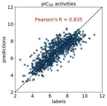
Figure 1: Correlation analysis between true and predicted pIC₅₀.

Epidermal Growth Factor Receptor (EGFR; ErbB-1) is a protein target found on the surface of some cells and to which epidermal growth factor binds, causing the cells to divide excessively. ErbB-1 are found in many human cancers, and their over-expression or constitutive activation may be critical factors in the development and malignancy of these tumors. Inhibition of ErbB pathways with targeted agents has been shown to be validated anti-cancer therapy.

In order to discover new inhibitors to the target ErbB-1, we use pIC₅₀ to measure the potency of a molecule in inhibiting ErbB-1. Accurate prediction of the pIC₅₀ can significantly accelerate the drug design process, as no in vitro determination of pIC₅₀ is needed. We extracted 7,698 molecules with pIC₅₀ value from the ChEMBL database Gaulton et al., (2011) in total. The retained dataset contains molecules with up to 100 heavy atoms. We randomly select 1000 samples for validation, 1000 samples for testing, and the remaining for training. We follow the same setting as in Sec. 4.1 except the number of the target property is one. Besides MAE, we also report the Pearson’s correlation coefficient ($R\in[-1,1]$) between the true and predicted pIC₅₀ in Table 4. A higher R represents the predicted value being more positively correlated with the true value.

Molecular graphs in real-world drug discovery task are generally large and of high diversity. From Table 4, we observe that our proposed IGNN is able to predict pIC₅₀ with $R=0.835$ and $\text{MAE}=0.6174$, achieving the best perfomrance. The illustration of the correlation analysis for IGNN is depicted in Figure 1. Our experimental study shows that IGNN works well in such complex setting, verifying the importance of information maximization on edges.

5 Conclusions

In this work, we designed an Information Maximizing Graph Neural Networks (IGNN) to maximize the mutual information between edge feature vectors and transform matrices. Currently, no other GNN variants utilize the edge information as efficiently as IGNN. The key element critical to IGNN’s success is the reformulation of the mutual information as a differentiable objective by adopting a variational approach. We tested IGNN in various scenarios including quantum property regressions and drug discovery. The promising results demonstrated the effectiveness of IGNN.

References

- Agakov, (2004) Agakov, D. B. F. (2004). The im algorithm: a variational approach to information maximization. NeurIPS.
- Barber and Agakov, (2006) Barber, D. and Agakov, F. V. (2006). Kernelized infomax clustering. In NeurIPS.
- Bridle et al., (1992) Bridle, J. S., Heading, A. J., and MacKay, D. J. (1992). Unsupervised classifiers, mutual information and’phantom targets. In NeurIPS.
- Chen et al., (2016) Chen, X., Duan, Y., Houthooft, R., Schulman, J., Sutskever, I., and Abbeel, P. (2016). Infogan: interpretable representation learning by information maximizing generative adversarial nets. In NeurIPS.
- Cho et al., (2014) Cho, K., Van Merriënboer, B., Bahdanau, D., and Bengio, Y. (2014). On the properties of neural machine translation: Encoder-decoder approaches. arXiv preprint arXiv:1409.1259.
- Defferrard et al., (2016) Defferrard, M., Bresson, X., and Vandergheynst, P. (2016). Convolutional neural networks on graphs with fast localized spectral filtering. In NeurIPS.
- Duvenaud et al., (2015) Duvenaud, D. K., Maclaurin, D., Iparraguirre, J., Bombarell, R., Hirzel, T., Aspuru-Guzik, A., and Adams, R. P. (2015). Convolutional networks on graphs for learning molecular fingerprints. In NeurIPS.
- Gaulton et al., (2011) Gaulton, A., Bellis, L. J., Bento, A. P., Chambers, J., Davies, M., Hersey, A., Light, Y., McGlinchey, S., Michalovich, D., Al-Lazikani, B., et al. (2011). Chembl: a large-scale bioactivity database for drug discovery. Nucleic acids research, 40(D1):D1100–D1107.
- Gilmer et al., (2017) Gilmer, J., Schoenholz, S. S., Riley, P. F., Vinyals, O., and Dahl, G. E. (2017). Neural message passing for quantum chemistry. In ICML.
- Gori et al., (2005) Gori, M., Monfardini, G., and Scarselli, F. (2005). A new model for learning in graph domains. In Proceedings. 2005 IEEE International Joint Conference on Neural Networks, 2005., volume 2, pages 729–734. IEEE.
- Grover and Leskovec, (2016) Grover, A. and Leskovec, J. (2016). node2vec: Scalable feature learning for networks. In Proceedings of the 22nd ACM SIGKDD international conference on Knowledge discovery and data mining, pages 855–864. ACM.
- Hamilton et al., (2017) Hamilton, W., Ying, Z., and Leskovec, J. (2017). Inductive representation learning on large graphs. In NeurIPS, pages 1024–1034.
- Hjelm et al., (2019) Hjelm, R. D., Fedorov, A., Lavoie-Marchildon, S., Grewal, K., Trischler, A., and Bengio, Y. (2019). Learning deep representations by mutual information estimation and maximization. In ICLR.
- Kingma and Ba, (2014) Kingma, D. P. and Ba, J. (2014). Adam: A method for stochastic optimization. arXiv preprint arXiv:1412.6980.
- Kingma and Welling, (2013) Kingma, D. P. and Welling, M. (2013). Auto-encoding variational bayes. arXiv preprint arXiv:1312.6114.
- Kipf and Welling, (2017) Kipf, T. N. and Welling, M. (2017). Semi-supervised classification with graph convolutional networks. In ICLR.
- Krause et al., (2010) Krause, A., Perona, P., and Gomes, R. G. (2010). Discriminative clustering by regularized information maximization. In NeurIPS.
- Lanczos, (1950) Lanczos, C. (1950). An iteration method for the solution of the eigenvalue problem of linear differential and integral operators. United States Governm. Press Office Los Angeles, CA.
- Li et al., (2016) Li, Y., Tarlow, D., Brockschmidt, M., and Zemel, R. (2016). Gated graph sequence neural networks. In ICLR.
- Liao et al., (2019) Liao, R., Zhao, Z., Urtasun, R., and Zemel, R. S. (2019). Lanczosnet: Multi-scale deep graph convolutional networks. In ICLR.
- Ramakrishnan et al., (2014) Ramakrishnan, R., Dral, P. O., Rupp, M., and Von Lilienfeld, O. A. (2014). Quantum chemistry structures and properties of 134 kilo molecules. Scientific data, 1:140022.
- Scarselli et al., (2009) Scarselli, F., Gori, M., Tsoi, A. C., Hagenbuchner, M., and Monfardini, G. (2009). The graph neural network model. IEEE Transactions on Neural Networks, 20(1):61–80.
- Schlichtkrull et al., (2018) Schlichtkrull, M., Kipf, T. N., Bloem, P., Van Den Berg, R., Titov, I., and Welling, M. (2018). Modeling relational data with graph convolutional networks. In European Semantic Web Conference, pages 593–607. Springer.
- Veličković et al., (2018) Veličković, P., Cucurull, G., Casanova, A., Romero, A., Lio, P., and Bengio, Y. (2018). Graph attention networks. In ICLR.
- Veličković et al., (2019) Veličković, P., Fedus, W., Hamilton, W. L., Liò, P., Bengio, Y., and Hjelm, R. D. (2019). Deep graph infomax. In ICLR.
- Vinyals et al., (2015) Vinyals, O., Bengio, S., and Kudlur, M. (2015). Order matters: Sequence to sequence for sets. arXiv preprint arXiv:1511.06391.
- Xu et al., (2019) Xu, K., Hu, W., Leskovec, J., and Jegelka, S. (2019). How powerful are graph neural networks? In ICLR.
- Ying et al., (2018) Ying, Z., You, J., Morris, C., Ren, X., Hamilton, W., and Leskovec, J. (2018). Hierarchical graph representation learning with differentiable pooling. In NeurIPS, pages 4800–4810.