Order parameter dynamics of the non-linear sigma model in the large $N$ limit

Abstract

We study non-equilibrium order parameter dynamics of the non-linear sigma model in the large $N$ limit, using Keldysh formalism. We provide a scheme for obtaining stable numerical solutions of the Keldysh saddle point equations, and use them to study the order parameter dynamics of the model either following a ramp, or in the presence of a periodic drive. We find that the transient dynamics of the order parameter in the presence of a periodic drive is controlled by the drive frequency displaying the phenomenon of synchronization. We also study the approach of the order parameter to its steady state value following a ramp and find out the effective temperature of the steady state. We chart out the steady state temperature of the ordered phase as a function of ramp time and amplitude, and discuss the relation of our results to experimentally realizable spin models.

I Introduction

The study of quantum field theoretic systems driven out of equilibrium has received a lot of interest, both in the context of high energy physics and ultracold atom systems sdas1 ; sdas2 ; sengupta1 ; polkovnikov1 ; rigol1 . There are several reasons for such a surge of interest in this field. The first is the recent experimental realizability of isolated quantum systems using suitable combination of lasers and ultracold atoms. Such a setup may emulate strongly correlated condensed matter models isolated from its environment. The low energy properties of such correlated systems are often described by quantum field theories. Furthermore, the parameters of these ultracold atom systems are easily tunable; therefore they serve as perfect test beds for studying quantum dynamics of these models. The study of quantum field theories driven out of equilibrium is therefore expected to provide relevant input for understanding such experimental systems. The second motivation is more theoretical in nature and involves developing an understanding of non-equilibrium dynamics of quantum field theoretic systems. An example of such endeavor involves the study of the rate of excitation production in such systems due to the presence of the drive. Such studies are particularly interesting near the critical points of these models and in the presence of a linear or a periodic drive. The former type of drives leads to the well-known Kibble-Zurek (KZ) scaling kz1 ; anatoli1 ; ks1 , and the latter leads to a realization of Stückleberg interference phenomenon in these systems stu1 ; ks2 . In addition, the study of such system allows us to address the notion of universality in such out-of-equilibrium systems, whose details may differ significantly from their equilibrium counterpart rg1 ; ks3 .

Moreover, there are two other broad theoretical motivations for studying such dynamics in field theoretic models. The first of them involves understanding the transient dynamics of a driven field theory. Such dynamics can in principle be complicated due to the interplay of the drive frequency with several inherent frequency scales of the model (arising out of its mass and interaction parameters). The second involves the approach of such a driven system to its steady state and eventual onset of thermalization. It is usually expected that for a non-integrable model, such a steady state would be thermal and shall thus be characterized by an effective temperature rigol1 . These issues have been studied recently in the context of the SYK model syk1 . However, the dependence of this effective temperature on the drive amplitude and frequency is a model dependent phenomenon, and has not been widely studied for non-integrable quantum field theories beyond $d=1$ cardyref1 .

The study of out-of equilibrium dynamics in interacting field theories, however, is technically challenging even at zero temperature. The difficulty involved stems from the fact that the properties of the driven system may depend, in principle, on all its states. This situation is to be contrasted with the study of equilibrium field theories, where one requires the knowledge of the ground state of the theory, which can be computed using several known perturbative techniques. For this reason, most of the studies on dynamics of such field theories have concentrated on free field theories which are integrable. Such studies are interesting in their own right and lead to a wealth of information about dynamical aspects of several systems ft1 . However, several properties of such integrable field theories are fundamentally different from their non-integrable counterparts. One key example involves the property of steady states that the driven system reaches at sufficiently long time; for integrable theories, such states are not necessarily thermal and are described by a generalized Gibbs ensemble (GGE). In contrast, the steady state of driven non-integrable models are usually thermal in accordance with the eigenstate thermalization hypothesis (ETH) ethlit . However a detailed study of such steady state behavior for $d>1$ quantum field theoretical systems turns out to be difficult.

In this work, we carry out such a study for quantum rotors described by the non-linear sigma model in the large $N$ limit subir1 . This model serves as an effective description for several spin systems sref1 . Moreover, it is conjectured to be dual to higher spin gauge theories in $AdS_{4}$ hspinref1 . It is well known that such higher spin gauge theories are often intractable; thus we expect the study of non-equilibrium dynamics of the more tractable large $N$ vector model to provide useful information about several dynamic properties of its dual counterpart. The dynamics of the paramagnetic phase of this model has been studied in Ref. sdas3, . Here, we concentrate on the ordered phase of the model, and study the behavior of its order parameter, either following a ramp or in the presence of a periodic drive. Such a drive or ramp is implemented by making the coupling parameter of the model time-dependent. In this work, we always restrict ourselves to the case where we are within the ordered phase at all times, and are sufficiently away from the critical point.

The main results of our work are as follows. First, we set the Keldysh saddle point equations for the driven model and provide a prescription for obtaining stable numerical solutions of these equations. We find that our numerical method leads to stable convergent solutions for the order parameter dynamics as long as the drive or ramp amplitude is sufficiently small. Second, using this method, we study the long time steady state behavior of the order parameter following a ramp. We study the approach of the order parameter to its steady state value and compute the effective temperature ${\mathcal{T}}_{\mathrm{eff}}$ of the steady state. We chart out this effective temperature as a function of the ramp time and amplitude. Third, we study the transient dynamics of the order parameter in the presence of a periodic drive. We find that the transient dynamics is controlled by the drive frequency and the order parameter oscillation displays synchronization. We explain the reason for such synchronization using the large $N$ Keldysh saddle point equation of motion. Finally, we discuss our main results and point out their experimental implications.

The plan of the rest of the paper is as follows. In Sec. II, we study the dynamics of the large $N$ non-linear sigma model using Keldysh formalism and chart out our numerical method. This is followed by Sec. III where we present our main results for periodic drive and quench dynamics. Finally, we discuss our main results and conclude in Sec. IV.

II General formalism

In this section, we first set up the Keldysh formalism following the treatment of the paramagnetic phase of the model in Ref. sdas3, , and obtain the saddle point equations of the order parameter in Sec. II.1. This is followed by a prescription for an efficient numerical solution of these saddle point equations in Sec. II.2.

II.1 Quench dynamics in the ferromagnetic phase

The action of the large $N$ non-linear sigma model in equilibrium is given by subir1

$$S[\phi^{\ast},\phi]=\int d^{d}x\,dt\left[\frac{N}{2\,g(t)}(\partial_{\mu}{{\mathbf{\phi}}}({{\mathbf{x}}},t))\cdot(\partial^{\mu}{{\mathbf{\phi}}}({{\mathbf{x}}},t))+\lambda({{\mathbf{x}}},t)\left({{\mathbf{\phi}}}\cdot{{\mathbf{\phi}}}-1\right)\right],$$ (1)

where ${{\mathbf{\phi}}}({{\mathbf{x}}},t)$ is an $N$ dimensional vector with real components. In the large $N$ limit, $N\rightarrow\infty$ while $g(t)$ remains finite ($O(1)$). The field $\lambda({{\mathbf{x}}},t)$ is a Lagrange multiplier which imposes the constraint ${{\mathbf{\phi}}}({{\mathbf{x}}},t)\cdot{{\mathbf{\phi}}}({{\mathbf{x}}},t)=1$. The saddle point equation of the model implements this constraint on the average, and leads to a solution with uniform $\lambda$. It is well known that the critical coupling at equilibrium is given by:

$$\frac{1}{g_{c}({\mathcal{T}})} = \int\frac{d^{d}k}{(2\pi)^{d}}\frac{\coth\left(\beta\,k\right)}{2\,k}\,,$$ (2)

where $k=|{\mathbf{k}}|$, $\mathcal{T}$ is the temperature, $\beta=1/{\mathcal{T}}$, and we have set the velocity $c=1$.

In this work, we are going to concentrate on the magnetically ordered phase which occurs at $g<g_{c}$. In this phase, we write $\phi=(\rho,\Pi_{1},\Pi_{2},\cdots,\Pi_{N-1})$ to allow for a finite expectation value $\rho$ of one of the components of the vector field $\phi$: $\langle\phi_{1}\rangle=\rho$. In equilibrium, the magnetization $\rho$ is a constant; however, a time-dependent $g(t)$ is expected to lead to a time-dependence of $\rho$. Also, we note that we shall discuss global protocols in this work, which allow $\rho$ to be independent of space. The action in the ordered phase in the presence of the drive is then given by

$$S=\int d^{d}x\,dt\left[\frac{N}{2\,g(t)}\Big{\{}(\partial_{\mu}\Pi({{\mathbf{x}}},t))\cdot(\partial^{\mu}\Pi({{\mathbf{x}}},t))+(\partial_{t}\rho(t))^{2}\Big{\}}+\lambda({{\mathbf{x}}},t)\left(\Pi\cdot\Pi+\rho^{2}-1\right)\right].$$ (3)

where $\Pi({{\mathbf{x}}},t)=(\Pi_{1},\Pi_{2},\cdots,\Pi_{N-1})$ is an $(N-1)$-dimensional vector with real components. In the large $N$ limit, $N\rightarrow\infty$ with $g(t)$ remaining $O(1)$. Redefining the fields as

$$\Pi\rightarrow{{\mathbf{\psi}}}=\sqrt{\frac{N}{g(t)}}\,\Pi\,,$$ (4)

the action becomes

$$S[\psi^{\ast},\psi]=\int dt{\mathcal{L}},\quad{\mathcal{L}}=\frac{1}{2}(\partial{{\mathbf{\psi}}})^{2}+\frac{N}{2g(t)}\dot{\rho}^{2}-\frac{1}{2}\Sigma({{\mathbf{x}}},t)\left({{\mathbf{\psi}}}^{2}+(\rho^{2}-1)\frac{N}{g(t)}\right)+\frac{N\alpha(t)}{g(t)}\,,$$ (5)

where

$$\alpha(t)=\frac{1}{4}\left[\frac{3}{2}\left(\frac{\dot{g}}{g}\right)^{2}-\left(\frac{\ddot{g}}{g}\right)\right],~{}~{}~{}~{}~{}~{}~{}~{}-\frac{1}{2}\Sigma({{\mathbf{x}}},t)=\frac{g(t)}{N}\lambda({{\mathbf{x}}},t)+\alpha(t)\,.$$ (6)

The last term in Eq. (5) is field independent, and can be therefore ignored. We note that we have ignored all total derivative terms in writing the expression for ${\mathcal{L}}$.

Following Ref. sdas3, , we express the partition function using the Schwinger-Keldysh path integral technique. This involves defining the fields $\psi_{+(-)}$ on the forward and backward contours. The partition function can be then written as

$${\mathcal{Z}}=\int{\mathcal{D}}{{\mathbf{\psi}}}_{\pm}{\mathcal{D}}\Sigma_{\pm}~{}e^{i\left[S({{\mathbf{\psi}}}_{+},\Sigma_{+})-S({{\mathbf{\psi}}}_{-},\Sigma_{-})\right]},$$ (7)

where $S[\psi_{\pm},\Sigma_{\pm}]\equiv S_{\pm}$ are given by Eq. (6), and are defined on the forward and backward Keldysh contours. Next, integrating out the fields ${{\mathbf{\psi}}}_{\pm}$ leads to the effective action for $\Sigma_{\pm}$ and $\rho_{\pm}$ as

$$S_{\mathrm{eff}} =\frac{(N-1)}{2}{\rm Tr}~{}\log(D^{-1})+N\int d^{d}x\,dt\,\frac{\dot{\rho}_{+}^{2}-\dot{\rho}_{-}^{2}}{2g(t)}-N\int d^{2}x\,dt\,\frac{\left(1-\rho^{2}_{+}(t)\right)\,\Sigma_{+}-\left(1-\rho^{2}_{-}(t)\right)\,\Sigma_{-}}{2g(t)}\,,$$ (8)

where $D$ is the propagator matrix whose inverse is

$$D^{-1}=\left(\begin{array}[]{cc}\partial^{2}-\Sigma_{+}&0\\ \vskip 6.0pt plus 2.0pt minus 2.0pt\cr 0&-\partial^{2}+\Sigma_{-}\end{array}\right)\,.$$ (9)

In the large $N$ limit, saddle point equations therefore take the form:

$$\frac{1-\rho^{2}_{+}(t)}{g(t)}=-{\rm Tr}~{}D_{++}\,,~{}~{}~{}~{}~{}~{}~{}\frac{1-\rho^{2}_{-}(t)}{g(t)}={\rm Tr}~{}(D_{--})\,,$$

$$\rho_{+}\,\Sigma_{+}=\ddot{\rho}_{+}\,,\quad\rho_{-}\,\Sigma_{-}=\ddot{\rho}_{-}\,,$$ (10)

where $D^{-1}_{++}=\partial^{2}-\Sigma_{+}$ and $D^{-1}_{--}=-\partial^{2}+\Sigma_{-}$. At the saddle point, we should have $\rho_{+}=\rho_{-}=\rho$ and $\Sigma_{+}=\Sigma_{-}=\Sigma$, similar to the structure in the paramagnetic phase. This means we need to solve the two coupled equations:

$$1-\rho^{2}(t)=g(t)\,{\rm Tr}~{}\mathcal{D}\,,\quad\rho(t)\,\Sigma(t)=\ddot{\rho}(t)\,,$$

$$\mathcal{D}=-D_{++}=D_{--}\,.$$ (11)

Following Ref. sdas3, , the first of the two coupled equations can be written as:

$$\rho^{2}(t)+g(t)\int\frac{d^{d}k}{(2\pi)^{d}}\frac{1}{2\,\Omega_{k}(t)}\coth\left(\frac{\beta\,k}{2}\right) = 1\,,$$ (12)

where $\Omega_{k}(t)$ satisfies the equation:

$$\frac{1}{2}\frac{\ddot{\Omega}_{k}}{\Omega_{k}}-\frac{3}{4}\left(\frac{\dot{\Omega}_{k}}{\Omega_{k}}\right)^{2}+\Omega_{k}^{2}=k^{2}+\Sigma(t)\,.$$ (13)

In equilibrium, we have $\dot{\rho}=0$. Therefore, the saddle has $\Sigma_{+}=\Sigma_{-}\equiv 0$ for, say, when $g=$constant in the ordered phase with non-zero $\rho$, and the other equation to solve is:

$$\rho^{2}+g\,\int d^{d}x~{}\langle{{\mathbf{x}}},t|D|{{\mathbf{x}}},t\rangle_{\beta}=1\,.$$ (14)

However, here we seek a solution such that $g(t)$, and hence $\Omega_{k}(t)$, are slowly-varying functions of $t$. Let us assume an expansion

$$\rho(t) = \sum\limits_{n=0}^{\infty}\epsilon^{n}\,\rho^{(n)}(t)\,,\quad\Omega_{k}(t)=\sum\limits_{n=0}^{\infty}\epsilon^{n}\,\Omega_{k}^{(n)}(t)\,.$$ (15)

The initial conditions are: $\Sigma(0)=0$ so that $\rho(0)=\sqrt{1-g(0)/g_{c}({\mathcal{T}},t=0)}$, and $\dot{\rho}(0)=0$. We note that a time-dependent $g$ generates a non-zero $\Sigma(t)$, which is not necessarily small. Nevertheless, for protocols with small $\omega$, $\dot{\Sigma}$ is expected to be small [${\rm O}(\epsilon)$]. This implies that $\dot{\Omega}_{k}$ and $\ddot{\Omega}_{k}$ are ${\rm O}(\epsilon)$ and ${\rm O}(\epsilon^{2})$, respectively. It is only under this condition that one can consider the derivative terms in $\Omega_{k}(t)$ as higher order. Performing an expansion and collecting all terms with the same order in $\epsilon$, we find, at zeroth order,

$$\Omega_{k}^{(0)}(t) = \sqrt{k^{2}+\Sigma(t)},\,\,\dot{\Omega}_{k}^{(0)}=\frac{\dot{\Sigma}}{2\sqrt{k^{2}+\Sigma}},\,\,\ddot{\Omega}_{k}^{(0)}=\frac{\ddot{\Sigma}}{2\sqrt{k^{2}+\Sigma}}-\frac{\dot{\Sigma}^{2}}{4\,(k^{2}+\Sigma)^{3/2}}.$$ (16)

Then using these in Eq.  13 at next order, we get:

$$\frac{1}{\Omega_{k}}=\frac{1}{\sqrt{k^{2}+\Sigma^{2}}}\Big{[}1+\frac{\ddot{\Sigma}}{8\,(k^{2}+\Sigma)^{2}}-\frac{5\,\dot{\Sigma}^{2}}{32\,(k^{2}+\Sigma)^{3}}\Big{]}\,.$$ (17)

Thus one can develop a systematic perturbative expansion of the saddle point equations for small $\omega$. We shall, however, be interested in behavior of the system beyond this regime. Thus in Sec. II.2 we develop a prescription for exact numerical solution of the saddle point equations.

II.2 Numerical solution of the saddle point equations

In this section, we provide a numerically efficient prescription to solve Eqs. (12) and (13). In what follows, we shall focus on $d=3$, for which the ordered phase exists at finite temperatures. We first consider the initial condition: $\dot{\rho}=0,\Sigma=0$ at $t=0$. From the discussion regarding the zeroth order solution (before Eq. (17)), it becomes clear that one has $\Omega_{k}(0)=k$ and $\dot{\Omega}_{k}(0)=\frac{\dot{\Sigma}(0)}{2\,k}$. At this point, we note two essential points. First, for numerical solution of these equations, it is useful to have an initial condition for $\dot{\Sigma}(0)$ which we shall take to be a small initial value. The qualitative features of our numerical results would not depend on the precise value of $\dot{\Sigma}(0)$. Second, since we are in $d=3$, the coupling has the dimension of mass. For numerical calculations, we rescale all length and time scales by $\sqrt{g_{c}(0)}$, where $g_{c}(0)$ is the zero temperature critical coupling value at equilibrium and hereafter we will set $g_{c}(0)=1$.

We start with a zero initial temperature where the system is in its ground state. One can then write a set of three self-consistent equations that we need to solve. These are given by

$$\rho^{2}(t)+g(t)\int\frac{d^{3}k}{(2\pi)^{3}}\frac{1}{2\,\Omega_{k}(t)}=1\,,$$

$$\frac{1}{2}\frac{\ddot{\Omega}_{k}}{\Omega_{k}}-\frac{3}{4}\left(\frac{\dot{\Omega}_{k}}{\Omega_{k}}\right)^{2}+\Omega_{k}^{2}=k^{2}+\frac{\ddot{\rho}(t)}{\rho(t)}\,,$$

$$g(t)=g_{0}+\left(g_{1}-g_{0}\right)\zeta(t)\,,$$ (18)

where $g_{0}=g(t=0)$, and $\zeta(t)$ is a function of time that satisfies $\zeta(0)=0$. The form of the second equation suggests the introduction of new variables:

$$\rho(t)\equiv\rho(0)\,e^{D(t)}\,,\quad\Omega_{k}(t)\equiv k\,e^{B_{k}(t)}\,,$$ (19)

with initial conditions $D(0)=B_{k}(0)=0$. Taking derivatives, we get:

$$\ddot{\rho}(t) = \rho(t)\left[\ddot{D}(t)+\dot{D}^{2}(t)\right],\quad\dot{\Omega}_{k}(t)=\Omega_{k}(t)\dot{B}_{k}(t),\quad\ddot{\Omega}_{k}(t)=\Omega_{k}(t)\left[\ddot{B}_{k}(t)+\dot{B}_{k}^{2}(t)\right].$$ (20)

Using these, the second equation of Eq. (18) transforms into (omitting time arguments for simplicity)

$$\ddot{B}_{k}-\frac{1}{2}\dot{B}_{k}^{2}+2k^{2}\left(e^{2B_{k}}-1\right)=2\left[\ddot{D}+\dot{D}^{2}\right]\,.$$ (21)

We transform the above second order ordinary differential equation (ODE) to first order ODEs, by introduction of a new set of variables, namely,

$$\chi_{k} = \dot{B}_{k}\,,\quad\nu=\dot{D}\,.$$ (22)

The new equation takes the form:

$$\dot{\chi}_{k}-\frac{\chi^{2}_{k}}{2}+2\,k^{2}\left(e^{2\,B_{k}}-1\right)=2\left[\dot{\nu}+\nu^{2}\right].$$ (23)

Using a simple central difference scheme with discretized time and step size $\Delta t$:

$$f^{\prime}(n)=\frac{f(n+1)-f(n-1)}{2\Delta t}+\mathcal{O}\left(\Delta t^{2}\right),$$ (24)

the ODEs read (the time arguments are shifted for convenience):

$$B_{k}(n+1)-B_{k}(n-1) = 2\,\Delta t\,\chi_{k}(n)\,$$

$$D(n+1)-D(n-1) = 2\Delta t\,\nu(n)\,,$$ (25)

$$\chi_{k}(n)-\chi_{k}(n-2)-\Delta t\left[\chi_{k}^{2}(n-1)+4k^{2}\left(1-e^{2\,B_{k}\,(n-1)}\right)\right] = 2\,\nu(n)-2\,\nu(n-2)+4\,\Delta t\,\nu^{2}\,(n-1)\,.$$

In order to fulfill the constraint equation, we seek an equation of the form $B_{k}(n,D(n))$. Inserting the second expressions for $\nu(n)$ into the last equation of Eq. (25), we get:

$$\chi_{k}(n) = \chi_{k}(n-2)+\Delta t\,\chi_{k}^{2}(n-1)+4\,\Delta t\,k^{2}\left(1-e^{2B_{k}(n-1)}\right)$$ (26)

$$+2\,\frac{D(n+1)-D(n-1)}{2\Delta t}-2\,\nu\,(n-2)+4\,\Delta t\,\nu^{2}\,(n-1)\,.$$

Using Eqs. (25) and (26), for $B_{k}(n)$, we obtain:

$$B_{k}(n) = \left[B_{k}(n-2)+2\,D(n)-2\,D(n-2)\right]+2\,\Delta t\left[\chi_{k}\,(n-3)-2\,\nu\,(n-3)\right]$$ (27)

$$\quad+2\,\Delta t^{2}\left[\chi_{k}^{2}\,(n-2)+4\,k^{2}\left(1-e^{2B_{k}(n-2)}\right)+4\,\nu^{2}\,(n-2)\right].$$

Note that the term $\propto\Delta t^{2}k^{2}$ in Eq. (27) is small for sufficiently small $\Delta t$ and for the k modes which participate in the dynamics till the time we carry out the numerics.

The equation for the constraint can be written in terms of $\rho(n)$ as

$$\rho^{4}(n)-\rho^{2}(n)+\tilde{G} = 0\,,\quad\tilde{G}=\frac{g(n)}{(2\,\pi)^{3}}\int_{0}^{\Lambda}d^{3}{k}\,\frac{\rho^{2}(0)}{2\,k}\,e^{2D(n)-B_{k}(n,D(n))}\,,$$ (28)

where $\Lambda=\sqrt{8\pi^{2}}$ is the ultraviolet cutoff. The last equation can be solved symbolically in terms of $\tilde{G}$. It yields:

$$\rho^{2}(n)=\frac{1}{2}\left[1\pm\sqrt{1-4\,\tilde{G}}\right].$$ (29)

Hence, the integration for $\tilde{G}$ has to be performed only once per time step. The sign of the solution is chosen such that $\Delta\rho(n)\equiv|\rho(n)-\rho(n-1)|$ is minimized. The condition $4\,\tilde{G}\leq 1$ must be fulfilled at all times. This restricts the validity of this approach to quenches or drives which keep the system well within the ordered phase.

The initial conditions $\left(\ddot{\rho}(0)=\dot{\rho}(0)=\ddot{\Omega}_{k}(0)=\dot{\Omega}_{k}(0)=0\right)$ are chosen to be:

$$\rho_{0} = \sqrt{1-\frac{g(0)}{g_{c}}}\,,\quad\chi_{k}(0)=\chi_{k}(1)=0\,,\quad\nu(0)=\nu(1)=0\,,$$

$$B_{k}(2) = B_{k}(1)=B_{k}(0)=0\,,\quad D(2)=D(1)=D(0)=0\,.$$ (30)

The full problem has been reduced to a simple numerical integration and iteration per time step. This procedure can be computed very fast and at a low computational cost. In the next section, we shall use this computational procedure to study the dynamics of the order parameter in the presence of a periodic drive or following a sudden quench of $g$. We shall restrict our study here within the ordered phase for which $g(t)/g_{c}\leq 1/2$ at all times during the evolution; we have checked numerically that this is enough to ensure the stability of the above-mentioned procedure.

III Numerical Results

In this section, we chart out our numerical results, which involve two separate classes of studies. The first involves steady state of the driven system, while the second pertains to short-time transient dynamics.

Figure 1: Plot of the order parameter $\rho(t)$ as a function of $t/T$, showing approach of $\rho$ to its steady state value for $T=4$, $g_{i}/g_{c}=0.1$ and $g_{f}/g_{c}=0.45$. See text for details.

For addressing the steady state of this model, we use the following protocol. We drive the system using a drive protocol with time period $T$:

$$g(t)=g_{i}+(g_{f}-g_{i})\,\sin^{2}\left(2\,\pi\,t/T\right)$$ (31)

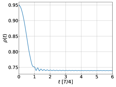
for $t\leq T/4\,,$ and then let the system evolve with a time independent Hamiltonian $H[g_{f}]$. This amounts to Hamiltonian evolution of the system following a ramp with a characteristic time $T$. One expects the system to reach a steady state in the course of such an evolution, and the goal of our study is to understand the behavior of the magnetization in this steady state. Here we choose the initial ($g_{i}$) and the final ($g_{f}$) values of the coupling such that $g(t)\leq g_{c}/2$ for all times; this ensures numerical stability as discussed in Sec. II.2. We track the evolution of the order parameter (magnetization) $\rho(t)$ during its subsequent evolution following the ramp. The behavior of $\rho(t)$, for $T=4$ and $g_{i}(g_{f})=0.1(0.45)g_{c}\,,$ is shown in Fig. 1. We find that $\rho(t)$ shows a fast decay (within $t\leq T/4$), and then displays small oscillations around a steady state value. The amplitude of these oscillations decay with $t$, and for $t\geq 10$, the magnetization reaches its steady state value. Thus we find a relatively fast onset of steady state behavior for order parameter dynamics of this model in its ordered phase. This behavior is to be contrasted with that in the paramagnetic phase, where such fast onset was not observed sdas3 .

Figure 2: Plot of the steady state value of $\rho$ as a function of the drive amplitude $(g_{f}-g_{i})/g_{c}$ and ramp time $T$, for $g_{i}/g_{c}=0.1$. The plot shows $\rho$ to be a monotonically decreasing function of the drive amplitude for any $T$ in the ordered phase. See text for details.

Figure 3: Plot of the steady state value of $\rho$ as a function of the ramp time $T$, for $g_{f}/g_{c}=0.45$ and $g_{i}/g_{c}=0.1$ (fixed). The plot shows that $\rho$ plateaus at large $T$. See text for details.

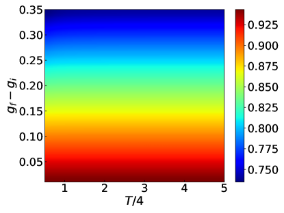
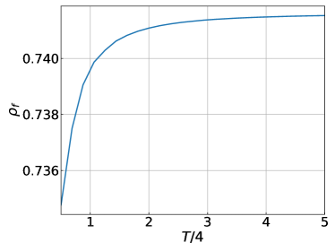
In Fig. 2, we plot the steady state order parameter value as a function of the ramp amplitude $\left(g_{f}-g_{i}\right)$ and the time period $T$, for $g_{i}/g_{c}=0.1$. We find that the steady state order parameter value is a monotonically decreasing function of the ramp amplitude. This behavior may be understood by noting that for any fixed $T$, a larger ramp amplitude amounts to pumping more energy in the system. Consequently, the steady state, which is a thermal state for non-integrable models, exhibits higher effective temperature for larger ramp amplitude. Both a larger $g_{f}$ and higher effective temperature lead to a lower steady state value of $\rho$. In contrast, we find that for a fixed $g_{f}-g_{i}$, the steady state value of $\rho$ is almost a constant within the range of $T$ studied. This feature is specifically pointed out in Fig. 3, where we find that the steady state value of $\rho$ plateaus to a constant value with increasing $T$. This is a consequence of the gapped nature of the system, leading to almost no energy absorption at low drive frequencies (large $T$).

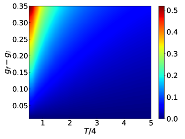
Next, in Fig. 4, we plot the effective temperature ${\mathcal{T}}_{\mathrm{eff}}$ of the steady state as a function of the ramp amplitude and $T$. ${\mathcal{T}}_{\mathrm{eff}}$ can be calculated from $\rho_{f}^{2}=1-g_{f}/g_{c}({\mathcal{T}}_{\mathrm{eff}})\,,$ with $\rho_{f}$ being the steady state value of $\rho$, and $g_{c}({\mathcal{T}}_{\mathrm{eff}})$ is obtained from Eq. (2). We find that ${\mathcal{T}}_{\mathrm{eff}}$ increases with both decreasing $T$ and large ramp amplitude. This behavior is expected since for gapped closed systems, efficient energy absorption can not occur at $T\geq[\Delta_{0}(g_{i})]^{-1}$, where $\Delta_{0}$ denotes the zero temperature equilibrium energy gap for $g=g_{i}$.

Figure 4: Plot of the effective temperature of the steady state as a function of $T$ and $(g_{f}-g_{i})/g_{c}$, for a fixed $g_{i}/g_{c}=0.1$. The plot shows that the effective temperature increases with decreasing $T$ and increasing drive amplitude. See text for details.

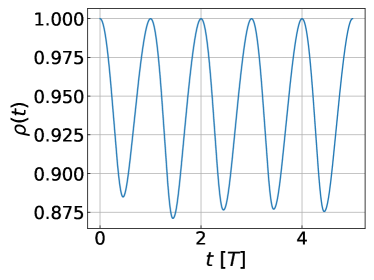
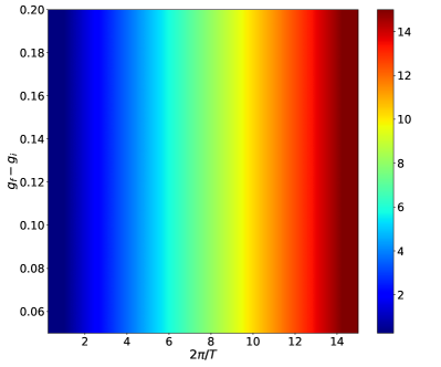
Finally, we discuss the transient dynamics of the model. For this, we drive the system using the protocol given by Eq. (31), and track the dynamics of the order parameter in the presence of the drive. The oscillation of the magnetization $\rho(t)$ is plotted in the left panel of Fig. 5 as a function of time. The right panel of Fig. 5 indicates the plot of the oscillation frequency of $\rho$ as a function of both drive amplitude and frequency. From these plots, we find that the oscillations have the same time period as the drive for a wide range of drive amplitudes and frequencies. This synchronization can be understood from our saddle point solution in the following manner. First, we note from Eq. (29), the dynamics of $\rho(t)$ is controlled by $\tilde{G}$. Next, from Eq. (28), we note that $\tilde{G}\sim g(t)$ at any instant. Moreover, from Eq. (27), it is easy to see that the exponent $\left[2\,D(n)-B(n,D(n))\right]$, which appears in $\tilde{G}$ within the integral is always small. This follows directly from Eq. (27), the boundary condition $B(0)=0$, and the fact that $\Delta t$ is always a small quantity. Consequently, the time dependence of $\tilde{G}$ is always controlled by $g$. Moreover, since we scale all quantities by the cutoff $\Lambda$, it is easy to see that $\tilde{G}\ll 1$ for any $g(t)$. As a result, one can expand $\sqrt{1-4\,\tilde{G}}\simeq 1-2\,\tilde{G}+O(\tilde{G}^{2})$. Thus, from Eq. (29), one finds that the time dependence of $\rho$ is essentially the same as that of $\tilde{G}$. Thus, synchronization occurs in this model as a structure of its saddle point equations, which governs the dynamics.

Figure 5: Left: Plot of the $\rho(t)$ as a function of $t/T$, for $(g_{f}-g_{i})/g_{c}=0.2$, $g_{i}/g_{c}=0$ and $T\in[2\,\pi/15,4\cdot 2\,\pi]$. The plot shows transient oscillations of $\rho$. Right: Plot of the oscillation frequency of $\rho$ as a function of drive amplitude and $2\,\pi/T$, indicating almost perfect synchronization. See text for details.

IV Discussion

In this work, we have studied the magnetization dynamics in the ordered phase of the non-linear sigma model within a large $N$ approximation, in the presence of either a ramp or a periodic drive. Our analysis uses Keldysh path integral techniques, and obtains the saddle point equations describing the magnetization dynamics. A key result of this work is to provide a scheme to obtain stable numerical solution of these saddle point equations. The method we chart out is effective in the ordered phase of the model as long as $g(t)/g_{c}<1/2$. We find that any further proximity to the critical points leads to numerical instability. Thus the dynamics of magnetization in such systems near the critical point still remains an open question which we leave for future study.

Using this method, we obtain several results regarding both transient dynamics and long-time steady states of the order parameter. For the former, we find that the oscillation of the magnetization synchronizes with the time period $T$ of the drive for all ranges of drive amplitudes. We tie this behavior to the structure of our saddle point equation, and show that this phenomenon is expected to be robust in the ordered phase. Such a robustness is confirmed in our numerical simulation for a wide range of $T$.

We also study the behavior of the steady states that the system reaches via evolution, subsequent to a ramp with characteristic time $T$. We find that the steady state is always thermal, and that the onset of thermalization occurs within a small value of of $t/T$. We compute the temperature of the steady state as a function of both the ramp time and the amplitude. We find that the steady state temperature increases with increasing ramp amplitude; in contrast, within the range of ramp times we study, it displays a relatively weak dependence on the ramp time $T$. The latter behavior can be attributed to the presence of a gapped spectrum in the ordered phase of the system.

There are several spin models which can be described under various approximations by such non-linear sigma model sref1 ; subir1 , within the large $N$ approximation. Such systems often have a large effective $S$ due to spin-orbit coupling, which makes them ideal candidates for large $N$ analysis. Our analysis indicates that the magnetization dynamics of such systems in the ordered phase should show fast approach to a thermal steady state for evolution, following a ramp. Moreover, the transient order parameter dynamics in the presence of a periodic drive would display synchronization.

To conclude, we have used the Keldysh technique to study non-equilibrium magnetization dynamics in the ordered phase of the non-linear sigma model within the large $N$ approximation. We have studied both transient dynamics of the order parameter in the presence of periodic drive, and its approach to a steady state following a ramp. Our results indicate that the transient order parameter oscillation synchronizes with the drive frequency. Moreover, the system evolves to a thermal steady state following a ramp, whose temperature is charted out as a function of the ramp time and the amplitude.

V Acknowledgments

We thank Subhodip Saha for participating in the initial stages of the project.

VI Author contribution statement

The author names in this paper are alphabetically ordered. All authors have equal contributions.

References

- (1)
- (2) A. Buchel, L. Lehner and R. C. Myers, JHEP 1208, 049 (2012); ibid, JHEP 1305, 067 (2013); A. Buchel, R. C. Myers and A. van Niekerk, Phys. Rev. Lett. 111, 201602 (2013); G. Mandal, R. Sinha and N. Sorokhaibam, JHEP 1508, 013 (2015); P. Basu, D. Das, S. R. Das, and T. Nishioka, JHEP 1303, 146 (2013).
- (3) S. R. Das, D. A. Galante and R. C. Myers, Phys. Rev. Lett. 112, 171601 (2014); ibid JHEP 1502, 167 (2015); ibid, JHEP 1508, 073 (2015); ibid JHEP 1605, 164 (2016); J. S. Cotler, M. P. Hertzberg, M. Mezei and M. T. Mueller, JHEP 1611, 166 (2016); P. Basu and S. R. Das Das, JHEP 2012, 103 (2012).
- (4) A. Polkovnikov, K. Sengupta, A. Silva, and M. Vengalla- tore, Rev. Mod. Phys. 83, 863 (2011);S. Mondal, D. Sen and K. Sengupta, Quantum Quenching, Anealing and Computation, Lecture notes in Physics, 802, 21 (2010); A Dutta, G Aeppli, BK Chakrabarti, U Divakaran, TF Rosenbaum, and D Sen, Quantum phase transitions in transverse field spin models : from statistical physics to quantum information, Cambridge, Cambridge University Press (2015)
- (5) J. Dziarmaga, Adv. Phys. 59, 1063 (2010); A. Lamacraft and J.E. Moore, Ultracold Bosonic and Fermionic Gases, Contemporary Concepts in Condensed Matter Science, Elsevier (Editors: A. Fletcher, K. Levin and D. Stamper-Kurn); M. Esposito, U. Harbola, and M.Mukamel, Rev. Mod. Phys. 81, 1665 (2009); M. Campisi, P. Hanggi, and P. Talkner, ibid. 83, 771 (2011).
- (6) M. Rigol, V Dunjko, and M Olshanii, Nature 452, 854 (2008).
- (7) T. W. B. Kibble, J. Phys. A 9, 1387 (1976); W. H. Zurek, Nature (London) 317, 505 (1985).
- (8) B. Damski, Phys. Rev. Lett. 95, 035701 (2005); A. Polkovnikov, Phys. Rev. B 72, 161201(R) (2005); C De Grandi, A Polkovnikov Quantum Quenching, Annealing and Computation, Lecture Notes in Physics, 802 75 (2010); A. Polkovnikov and V. Gritsev, Nature Phys. 4, 477 (2008).
- (9) K. Sengupta, D. Sen, and S. Mondal, Phys. Rev. Lett. 100, 077204 (2008); S. Mondal, D. Sen, and K. Sengupta, Phys. Rev. B 78, 045101 (2008); D. Sen, K. Sengupta, and S. Mondal, Phys. Rev. Lett. 101, 016806 (2008); S. Mondal, K. Sengupta, and D. Sen, Phys. Rev. B 79, 045128 (2009); D. Das, S. R. Das, D. A. Galante, R. C. Myers and K. Sengupta, JHEP 11 157 (2017).
- (10) E. C. G. Stueckelberg, Helv. Phys. Acta 5, 369 (1932); S. N. Shevchenko, S. Ashhab, and F. Nori, Phys. Reports 492, 1 (2010); W. D. Oliver, Y. Yu, J. C. Lee, K. K. Berggren, L. S. Levitov, and T. P. Orlando, Science 310, 1653 (2005); M. S. Rudner, A. V. Shytov, L. S. Levitov, D. M. Berns, W. D. Oliver, S. O. Valenzuela, and T. P. Orlando, Phys. Rev. Lett. 101, 190502 (2008), A. Dutta, A. Das, and K. Sengupta, Phys. Rev. E 92, 012104 (2015).
- (11) T. Kitagawa, E. Berg, M. Rudner, and E. Demler, Phys. Rev. B 82, 235114 (2010); N. H. Lindner, G. Refael, and V. Galitski, Nat. Phys. 7, 490 (2011); B. Mukherjee, A. Sen, D. Sen, and K. Sengupta, Phys. Rev B 94, 155122 (2016); B. Mukherjee, P. Mohan, D. Sen, K. Sengupta, Phys. Rev. B 97, 205415 (2018).
- (12) L. M. Sieberer, S. D. Huber, E. Altman, and S. Diehl, Phys. Rev. Lett. 110, 195301 (2013); S. de Sarkar, R. Sensarma, and K. Sengupta, J. Phys.: Condens. Matter 26, 325602 (2014);
- (13) M. Heyl, A. Polkovnikov, and S. Kehrein, Phys. Rev. Lett. 110, 135704 (2013); C. Karrasch and D. Schuricht, Phys. Rev. B 87, 195104 (2013); J. N. Kriel, C. Karrasch, and S.Kehrein, ibid. 90, 125106 (2014); S. Sharma, U. Divakaran, A. Polkovnikov, and A. Dutta, Phys. Rev. B 93, 144306 (2016).
- (14) A. Haldar, P. Haldar, I. Mandal, S. Banerjee, arXiv:1903.09652 (unpublished).
- (15) For a review see, P. Calabrese and J. Cardy, J. Phys A 42 504005 (2009); P Calabrese and J Cardy, Journal of Statistical Mechanics: Theory and Experiment, 06, P06002 (2004); ibid Journal of Statistical Mechanics: Theory and Experiment 06 P06008 (2007) (06).
- (16) A. Sen, S. Nandy, and K. Sengupta, Phys. Rev. B 94, 214301 (2016); ibid, J. Phys. A: Math. Theor. 51, 334002S (2018); S. Nandy, A.Sen, and D. Sen, Phys. Rev. X 7 031034 (2017); A. Lazarides, A. Das, and R Moessner, Phys. Rev. E 90, 012110 (2014); ibid Phys. Rev. Lett. 112, 150401 (2014).
- (17) For a review, see L. D’Alessio, Y. Kafri, A. Polkovnikov, and M. Rigol, Adv. Phys. 65, 239 (2016)
- (18) See for example Subir Sachdev, Quantum Phase Transition, Cambridge University Press (2011).
- (19) D.P. Arovas and A. Auerbach Phys. Rev. B 52, 10114 (1995); S. Pati, R.R.P. Singh, D.I. Khomskii Phys. Rev. Lett. 81, 5406, (1998).
- (20) I. R. Klebanov, A. M. Polyakov, Phys. Lett. B 550 213 (2002).
- (21) S. R Das and K. Sengupta, Journal of High Energy Physics 9, 72 (2012).