MASCARA-3b

We report the discovery of MASCARA-3b, a hot Jupiter orbiting its bright ($V=8.33$) late F-type host every $5.55149\pm 0.00001$ days in an almost circular orbit ($e=0.050^{+0.020}_{-0.017}$). This is the fourth exoplanet discovered with the Multi-site All-Sky CAmeRA (MASCARA), and the first of these that orbits a late-type star. Follow-up spectroscopic measurements were obtained in and out of transit with the Hertzsprung SONG telescope. Combining the MASCARA photometry and SONG radial velocities reveals a radius and mass of $1.36\pm 0.05$ $R_{\text{Jup}}$ and $4.2\pm 0.2$ $M_{\text{Jup}}$. In addition, SONG spectroscopic transit observations were obtained on two separate nights. From analyzing the mean out-of-transit broadening function, we obtain $v\sin i_{\star}=20.4\pm 0.4$ km s^-1. In addition, investigating the Rossiter-McLaughlin effect, as observed in the distortion of the stellar lines directly and through velocity anomalies, we find the projected obliquity to be $\lambda=1.2^{+8.2}_{-7.4}$ deg, which is consistent with alignment.

1 Introduction

With more than 4000 planets confirmed to date, the field of exoplanets has experienced a huge growth since the first detection two decades ago. This large number of discoveries has in particular been the product of extensive ground- and space-based transit photometry surveys, such as the missions of HAT (Bakos et al., 2004), WASP (Pollacco et al., 2006), CoRoT (Barge et al., 2008), Kepler (Borucki et al., 2010), and K2 (Howell et al., 2014). However, because of saturation limits, these surveys have for the most part been unable to monitor the brightest stars.

Transiting planets orbiting bright stars are important because these stars offer follow-up opportunities that are not available for fainter sources, allowing for detailed characterization of their atmosphere and the orbital architecture of the system. This includes the detection of water in the planetary atmosphere through high-resolution transmission spectroscopy (e.g., Snellen et al., 2010), for instance, and measurements of its spin-orbit angle through observations of the Rossiter-McLaughlin (RM) effect.

From space, the brightest exoplanet host stars are currently being probed thanks to the launch of TESS (Ricker et al., 2015), while ground-based projects with the same aims include KELT (Pepper et al., 2007) and the Multi-Site All-sky CAmeRA (MASCARA) survey (Talens et al., 2017b). The latter aspires to find close-in transiting giant planets orbiting bright stars that are well suited for detailed atmospheric characterization. This has so far led to the discovery and characterization of MASCARA-1, MASCARA-2, and MASCARA-4, three hot Jupiters orbiting A-type stars (Talens et al., 2017a, 2018b; Dorval et al., 2019).

In this paper we report the discovery and confirm and characterize MASCARA-3, the fourth planetary system found through the MASCARA survey. MASCARA-3b is a hot Jupiter with a 5.6-day period. It orbits a bright late F-type star ($V=8.33$). In Sect. 2 the discovery observations from MASCARA and the spectroscopic follow-up observations with SONG (Stellar Observation Network Group, Andersen et al., 2014) are described. The analysis and results for the host star are presented in Sect. 3, while Sect. 4 contains the investigation and characterization of its planet. The results are presented and discussed in Sect. 5.

2 Observations

In this section two different types of observations are presented: the MASCARA photometry, and the SONG spectroscopy (see Table 1).

MASCARA

The MASCARA survey is described in Talens et al. (2017b). In short, it consists of two instruments: one covering the northern sky at the Observatory del Roque de los Muchachos (La Palma, Spain), and one targeting the southern hemisphere located at the European Southern Observatory (La Silla, Chile). Each instrument consists of five wide-field CCDs that record images of the local sky throughout the night employing 6.4 s exposure times. Aperture astrometry is performed on all known stars brighter than $V=8.4$. The light-curves are extracted from the raw flux following the procedure described in Talens et al. (2018a), and transit events are searched for using the Box Least-Squares (BLS) algorithm of Kovács et al. (2002). MASCARA-3 has been monitored since early 2015 by the northern instrument, totalling more than 27247 calibrated photometric data points, each consisting of 50 binned 6.4 s measurements (i.e., 320 s per data point). A frequency analysis was performed on the light-curve measurements by computing its BLS periodogram, revealing a peak at a period of 5.55149 days. Phase-folding the light-curve using this period, we performed a preliminary analysis on the system and obtained parameter values that are useful for spectroscopic follow-up (see Table 2). The resulting phase-folded light-curve is shown in Fig. 1.

SONG

Succeeding the transit detection in the light-curve of MASCARA-3, follow-up spectroscopy was executed using the robotic 1-meter Hertzsprung SONG telescope (Andersen et al., 2019) at the Observatory del Teide (Tenerife, Spain). The observations were made in order to validate and characterize the planetary system. The telescope is equipped with a high-resolution echelle spectrograph that covers the wavelength range $4400-6900$Å. A total of 110 spectra were obtained between April 2018 and May 2019, employing a slit width of 1.2 arcsec that resulted in a resolution of $R\sim 77,000$. The exposure times have been varied between 600 and 1800 s. We used longer exposure time out of transits and shorter exposure times during transits to reduce phase smearing. Forty-five of the observations were gathered during two planetary transits that occurred on May 29, 2018, and November 28, 2018. For the first transit our spectroscopic observations cover the entire transit. However, due to bad weather, only a single spectrum was taken out of transit. On the second night we obtained a partial transit and post-egress spectra.

We planned to analyze the RM effect in this system using the Doppler tomography technique, therefore we did not use an iodine cell for observations taken during transit nights, but sandwiched each observation with ThAr exposures for wavelength calibration. From these spectra we obtained cross-correlation functions (CCFs) and broadening functions (BFs;  Rucinski, 2002). Spectra not taken during transit nights were obtained with an iodine cell inserted into the light path for high radial velocity (RV) precision.

The spectra and RV extraction was performed following Grundahl et al. (2017). The RV data points are estimated to have internal instrumental uncertainties of $\sim 31$ m sec^-1. The resulting RVs and their uncertainties are listed in Table 5.

Table 1: Observation log of MASCARA-3 containing the different types of observation, instrument, number of observations made, and observing dates.

Type	Inst.	No. of obs.	Obs. date
Phot.	MASCARA	27247	February 2015 – March 2018
RV Spec.	SONG	65	April 2018 – May 2019
RM Spec.	SONG	23	May 29, 2018
RM Spec.	SONG	22	Nov 28, 2018

Table 2: Best-fit values for the initial analysis of the MASCARA photometric data, with the eccentricity kept fixed at 0. Of these parameters, $P$ and $T_{0}$ were used as priors in the joint fit between the spectroscopy and phase-folded photometry.

Parameter	Value
Orbital period, $P$ (days)	5.55149$\pm 0.00002$
Time of mid-transit, $T_{0}$ (BJD)	2458268.455${}_{-0.003}^{+0.002}$
Total transit duration, $T_{14}$ (hr)	4.3$\pm 0.1$
Scaled planetary radius, $R_{\text{p}}/R_{\star}$	0.091$\pm 0.002$
Scaled orbital distance, $a/R_{\star}$	10.4${}_{-1.0}^{+0.4}$
Orbital inclination, $i$ (deg)	88$\pm 1.0$
Impact parameter, $b$	0.3$\pm 0.2$

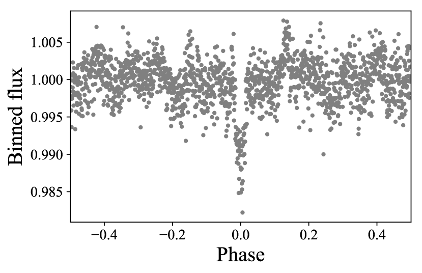
Figure 1: Calibrated and phase-folded MASCARA-3 photometry. The phase-folded data have been binned to 5 min. intervals, which reduced the number of data points from 27247 to 1596. The period of 5.55149 days used in the phase-folding is the highest peak obtained from constructing the BLS periodogram of the data.

3 Stellar characterization

We determined the spectroscopic effective temperature $T_{\rm eff}=6415\pm 110\,$K and metalliticy [Fe/H] $=0.09\pm 0.09\,$dex using SpecMatch-emp (Yee et al., 2017), classifying it as an F7 star. SpecMatch-emp compares the observed spectrum with an empirical spectral library of well-characterized stars. Using the BAyesian STellar Algorithm BASTA (Silva Aguirre et al., 2015) with a grid of BaSTI isochrones (Pietrinferni et al., 2004; Hidalgo et al., 2018), we combined the spectroscopically derived $T_{\rm eff}$ and [Fe/H] with the 2MASS $JHK$ magnitudes (see Table 3) and $Gaia$ DR2 parallax ($\pi=10.33\pm 0.11\,$mas) to obtain a final set of stellar parameters. Because the star is so close, we assumed zero extinction along the line of sight. In this way, we derived a stellar mass $M_{\star}=1.30^{+0.04}_{-0.03}M_{\sun}$, radius $R_{\star}=1.52^{+0.03}_{-0.02}R_{\sun}$, and stellar age $=2.8^{+0.5}_{-0.6}$ Gyr. We note that the uncertainties on the stellar parameters do not include systematic effects due to the choice of input physics in the stellar models. The model-dependent systematic uncertainties are at the level of a few percent.

Table 3: Literature and best-fit parameters for the stellar analysis of MASCARA-3. Sources: *Extracted from Gaia DR2 (Gaia Collaboration, 2018, https://gea.esac.esa.int/archive/). ^†Parameters from 2MASS (Cutri et al., 2003). ^‡From the Tycho catalog (Høg et al., 2000). The remaining parameter values are from this work.

Parameter	Value
Identifiers	HD 93148
Spectral type	F7
Right ascension, $\alpha$ (J2000.0)*	10${}^{\text{h}}$ 47${}^{\text{m}}$ 38.351${}^{\text{s}}$
Declination, $\delta$ (J2000.0)*	+71∘ 39′ 21.16′′
Parallax, $\pi$ (mas)*	10.3$\pm 0.1$
Distance (pc)*	97$\pm 1$
$V$-band mag., $V$†	8.33$\pm 0.01$
$J$-band mag., $J$‡	7.41$\pm 0.02$
$H$-band mag., $H$‡	7.20$\pm 0.04$
$K$-band mag., $K$‡	7.15$\pm 0.02$
Effective temperature, $T_{\text{eff},\star}$ (K)	$6415\pm 110$
Surface gravity $\log{\text{g}}_{\star}$ (cgs)	$4.18^{+0.01}_{-0.02}$
Metallicity, $[$Fe/H$]$ (dex)	$0.09\pm 0.09$
Age (Gyr)	$2.8^{+0.5}_{-0.6}$
Stellar mass, $M_{\star}$ ($M_{\sun}$)	$1.30^{+0.04}_{-0.03}$
Stellar radius, $R_{\star}$ ($R_{\sun}$)	$1.52^{+0.03}_{-0.02}$
Stellar density, $\rho_{\star}$ (g cm-3)	$0.52^{+0.04}_{-0.03}$

4 Photometric and spectroscopic analysis

The overall analysis of the photometry and RV data was made in a similar fashion as for MASCARA-1b (Talens et al., 2017a) and MASCARA-2b (Talens et al., 2018b) and is outlined in the following section. Because of the transit phase coverage and the low signal-to-noise ratio (S/N) of the RM detection, we modified our analysis for this data set accordingly. We give details on this in Sects. 4.2.1 and 4.2.2.

4.1 Joint photometric and RV analysis

The binned phase-folded MASCARA light-curve was modeled employing the model by Mandel & Agol (2002), using a quadratic limb-darkening law. The free parameters for the transit model were the orbital period ($P$), a particular mid-transit time ($T_{0}$), the semimajor axis scaled by the stellar radius ($a/R_{\star}$), the scaled planetary radius ($R_{p}/R_{\star}$), the orbital inclination ($i$), the eccentricity ($e$) and the argument of periastron ($\omega$), and finally, the quadratic limb-darkening parameters ($c_{1}$) and ($c_{2}$). For efficiency, the inclination, eccentricity, and argument of periastron were parameterized through $\cos i$, $\sqrt{e}\cos\omega$ and $\sqrt{e}\sin\omega$.

To model the RV observations, we only used spectra obtained with an iodine cell inserted in the light path (Table 5). This excludes data taken during transit nights. The RV data were compared to a Keplerian model where the stellar RV variations are caused by the transiting object. The additional parameters needed to describe the RV data are the RV semi-amplitude ($K$) and a linear offset in RV ($\gamma$). In addition, we allowed for a linear drift of the RV data points, $\dot{\gamma}$, caused by an unseen companion with a long period, for example.

To characterize the planetary system, we jointly modeled the the light-curve and the RVs. Because we fit to the phase-folded light-curve, we imposed Gaussian priors $P=5.55149\pm 0.00002$ days and $T_{0}=2458268.455^{+0.002}_{-0.003}$ BJD retrieved from the photometric analysis described in Sect. 2. In addition, we imposed Gaussian priors of $c_{1}=0.3797$ and $c_{2}=0.2998$ (Claret & Bloemen, 2011; Eastman et al., 2013) with conservative uncertainties of $0.1$. Furthermore, by using the spectroscopic value of the density $\rho_{\star}=0.52_{-0.03}^{+0.04}$ g cm^-3 as a prior, we constrained the orbital shape and orientation (see, e.g., Van Eylen & Albrecht, 2015, and references therein).

The log-likelihood for each data set is given as

$$\ln\mathcal{L}=-\dfrac{1}{2}\sum\limits_{i=1}^{N}\left(\ln\left(2\pi\left[\sigma_{i}^{2}+\sigma_{\text{jit}}^{2}\right]\right)+\dfrac{\left[O_{i}-C_{i}\right]^{2}}{\left[\sigma_{i}^{2}+\sigma_{\text{jit}}^{2}\right]}\right),$$ (1)

with $O_{i}$ and $C_{i}$ being the $i^{\prime}$th of $N$ data and model points in each data set. For the two data sets we introduced two jitter terms $\sigma_{\text{jit,p}}$ and $\sigma_{\text{jit,RV}}$ to capture any unaccounted noise. These jitter terms were added in quadrature to the internal errors $\sigma_{i}$ when we calculated the maximum likelihood. The total log-likelihood is the sum of Eq. 1 for the photometry and RV together with an additional likelihood term that accounts for priors.

The posterior distribution of the parameters was sampled through emcee, a Markov chain Monte Carlo (MCMC) multi-walker Python package (Foreman-Mackey et al., 2013). We initialized 200 walkers close to the maximum likelihood. They were evaluated for 10 000 steps, with a burn-in of 5000 steps that we disregard. By visually inspecting trace plots, we checked that the solutions converged at that point. In Table 4 we report the maximum likelihood values of the MCMC sampling. The quoted uncertainty intervals represent the range that excludes 15.85% of the values on each side of the posterior distribution, and the intervals encompass 68.3% of the probability. Figures 2 and 3 display the data and best-fit models for the joint analysis of the light-curve and the RVs. We note that the same analysis without a prior on the stellar density reveals results consistent within 1$\sigma$.

Table 4: Best-fitting and derived stellar, planetary, and system parameters for MASCARA-3. The parameters are extracted from the joint analysis of the photometry and RV (Sect. 4.1), the analysis of the mean out-of-transit BF (Sect. 4.2.1), the analysis of the grid of the shifted and binned Doppler shadow residuals (Sect. 4.2.2), and the analysis of the extracted RVs from the spectroscopic transit on the night of May 29, 2018 (Sect. 4.3).

Parameter	Value	Section
Fitting parameters
Quadratic limb darkening (MASCARA), ($c_{1}$, $c_{2}$)	($0.40\pm 0.07$, $0.31\pm 0.07$)	4.1
Systemic velocity, $\gamma$ (km s-1)	$-5.63\pm 0.01$	4.1
Linear trend in RV, $\dot{\gamma}$ (m s-1 yr-1)	$61\pm 19$	4.1
Orbital period, $P$ (days)	$5.55149\pm 0.00001$	4.1
Time of mid-transit, $T_{0}$ (BJD)	$2458268.455\pm 0.002$	4.1
Scaled planetary radius, $R_{\text{p}}/R_{\star}$	$0.092\pm 0.003$	4.1
Scaled orbital distance, $a/R_{\star}$	$9.5\pm 0.2$	4.1
RV semi-amplitude, $K_{\star}$ (m s-1)	$415\pm 13$	4.1
$\sqrt{e}\sin{\omega}$	$0.10^{+0.07}_{-0.09}$	4.1
$\sqrt{e}\cos{\omega}$	$0.20\pm 0.04$	4.1
$\cos i$	$0.042^{+0.012}_{-0.008}$	4.1
Jitter term phot., $\sigma_{\text{jit,p}}$	$0.0021\pm 0.0001$	4.1
Jitter term RV, $\sigma_{\text{jit,RV}}$ (km s-1)	$0.060\pm 0.008$	4.1
Quadratic limb darkening (SONG), ($c_{1,\text{s}}$, $c_{2,\text{s}}$)	($0.66\pm 0.09$, $0.40\pm 0.09$)	4.2.1
Microturbulence, $\beta$ (km s-1)	$4.3\pm 0.6$	4.2.1
Macroturbulence, $\zeta$ (km s-1)	$9.4\pm 0.4$	4.2.1
Proj. rotation speed (BF), $v\sin i_{\star}$ (km s-1)	$20.4\pm 0.4$	4.2.2
Jitter term RM out of transit, $\sigma_{\text{jit,out}}$ (m s-1)	$0.003\pm 0.002$	4.2.1
Proj. rotation speed (grid), $v\sin i_{\star}$ (km s-1)	$20.9\pm 3.2$	4.2.2
Projected obliquity (grid), $\lambda$ (deg)	$17.8\pm 20.0$	4.2.2
Impact parameter (grid), $b$	$0.30\pm 0.16$	4.2.2
3D rotation angles (deg)	($-1.4,-0.01,0.002$)	4.2.2
Proj. rotation speed (RV-RM), $v\sin i_{\star}$ (km s-1)	$20.3\pm 0.4$	4.3
Projected obliquity (RV-RM), $\lambda$ (deg)	$1.2^{+8.2}_{-7.4}$	4.3
Impact parameter (RV-RM), $b$	$0.39\pm 0.08$	4.3
RV offset on May 29, 2018, $\gamma_{{\text{RM}}}$ (km/sec)	$-15.181\pm 0.010$	4.3
Derived parameters (from the results in Sect. 4.1)
Orbital eccentricity, $e$	$0.050^{+0.020}_{-0.017}$
Argument of periastron, $\omega$ (deg)	$27^{+38}_{-27}$
Orbital inclination, $i$ (deg)	$87.6^{+1.0}_{-0.8}$
Impact parameter, $b$	$0.40\pm 0.10$
Total transit duration, $T_{14}$ (hr)	$4.55\pm 0.20$
Full transit duration, $T_{23}$ (hr)	$3.65\pm 0.23$
Semi-major axis, $a$ (au)	$0.067\pm 0.002$
Planetary mass, $M_{\text{p}}$ ($M_{\text{Jup}}$)	$4.2\pm 0.2$
Planetary radius, $R_{\text{p}}$ ($R_{\text{Jup}}$)	$1.36\pm 0.05$
Planetary mean density, $\rho_{\text{p}}$ (g cm-3)	$2.3\pm 0.3$
Equilibrium temperature, $T_{\text{eq}}$ (K)	$1473\pm 28$

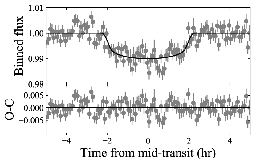
Figure 2: Phase-folded MASCARA-3 photometry data (gray) with the best-fit transit model (black) from the joint photometric and RV analysis. The corresponding best-fit parameters can be found in Table 4. The bottom plot displays the residuals.

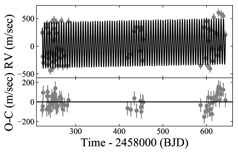
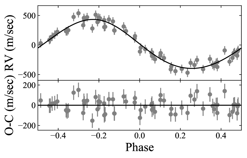
Figure 3: Radial velocity data from the SONG telescope (gray) with the best-fit Keplerian model (black) from the joint photometric and RV analysis. The data are plotted as a function of time (left) and phase-folded (right) to highlight that we allowed for the possibility of a linear trend in the RV. In the panel on the right side the best-fitting RV trend was removed from the data and model. The best-fit parameters are displayed in Table 4. The bottom plot shows the residuals.

4.2 Analyzing the stellar absorption line

We modeled the stellar absorption lines in a similar way as reported in Albrecht et al. (2007) and Albrecht et al. (2013). However, we modified our approach of comparing the model to the data because we found that the S/N of the BFs we created from our data was too low to be useful in determining $\lambda$ through an analysis of the RM effect. Nevertheless, they represent the width of the stellar absorption lines more faithfully than the CCFs, which have large wings (see Fig. 4). We were unable to determine the exact reason for this, but we suspect that the low S/N in the spectra is to blame. Determining the correct continuum level in spectra with low S/N and high resolution is extremely difficult. For the case of MASCARA-3, this problem is exacerbated by the fast stellar rotation and therefore wide stellar absorption lines. A mismatch in the continuum would lead to a low S/N in the derived BF. The same mismatch in the continuum correction would lead to enlarged wings in the CCFs. We therefore first obtained a measure for $v\sin i_{\star}$ by comparing our out-of-transit stellar line model to an average out-of-transit BF. We then analyzed the planet shadow in the transit data.

For the model with which we compared the out-of-transit and in-transit data we created a 201$\times$201 grid containing a pixelated model of the stellar disk. The brightness of each pixel on the stellar disk is scaled according to a quadratic limb-darkening law with the parameters $c_{1,\text{s}}$ and $c_{2,\text{s}}$ and set to zero outside the stellar disk. Each pixel was also assigned an RV assuming solid-body rotation and a particular projected stellar rotation speed, $v\sin i_{\star}$. The RVs of each pixel were further modified following the model for turbulent stellar motion as described in Gray (2005). This model has two terms. A microturbulence term that is modeled by a convolution with a Gaussian, whose $\sigma$ width we describe here with the parameter $\beta$. The second term in this model encompasses radial and tangential macroturbulent surface motion. We assign its $\sigma$ width the parameter $\zeta$. The modeled stellar absorption line was then obtained by disk integration. Finally, the Gaussian convolution also included the point spread function (PSF) of the spectrograph added in quadrature. We did not include convective blueshift in our model because the S/N of our spectra is low.

4.2.1 Out-of-transit stellar absorption line

To measure $v\sin i_{\star}$ we compared our out-of-transit line model to the BFs taken out of transit. We used only data from the second transit night because little data were obtained out of transit during the first transit night (Fig. 5). In addition to the five model parameters, $c_{1,\text{s}}$, $c_{2,\text{s}}$, $v\sin i_{\star}$, $\beta$, and $\zeta$, we also varied a jitter term $\sigma_{\text{jit,out}}$ during the fitting routine. We imposed Gaussian priors of $\beta=2.7$ km sec^-1 (Coelho et al., 2005) and $\zeta=6.1$ km sec^-1 (Gray, 1984), both with uncertainty widths of $0.5$ km sec^-1. The best-fit parameters were again found by maximizing the log-likelihood from Eq. 1 using emcee in the same way as in Sect. 4.1. The best-fit parameters are given in Table 4, and the data and best-fit model are shown in Fig. 4.

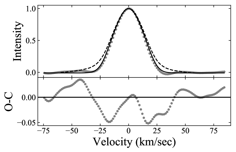
Figure 4: Mean out-of-transit BF (grey) with the best-fitting stellar absorption line model (black). For comparison the dashed line shows the mean out-of-transit CCF, which erroneously leads to an enlarged line width because of its wings, which we assume are caused by an imperfect normalization of the low S/N spectra (see Sect. 4.2).

4.2.2 The Doppler shadow

We observed spectroscopic transits during the nights of May 29, 2018, and November 28, 2018, to verify whether the companion is a planet orbiting the host star and to obtain the projected spin-orbit angle (or projected obliquity, $\lambda$) of the system. During transit, the planet blocks some of the star, which deforms the absorption line by reducing the amount of blue- or redshifted light that is visible to the observer at a particular phase of a transit. Subtracting the distorted in-transit absorption lines from the out-of-transit line will therefore reveal the planetary shadow that is cast onto the rotating stellar photosphere. For solid-body rotation this shadow travels on a line in a time-velocity diagram, and its zero-point in velocity and orientation depends on the projected obliquity and projected stellar rotation speed, as well as on the impact parameter. See Eq. 4 in Albrecht et al. (2011). The planet shadows we obtained during the two transit nights are shown in Fig. 5. Here we scaled and removed the average out-of-transit CCF from the second transit night from all observations. Clearly, MASCARA-3 b travels on a prograde orbit. During the first half of the transit, the distortion has negative RVs, and the RVs are positive during the second half of the transit. However, as our detection of the planet shadow has a low S/N, we did not strictly follow Albrecht et al. (2013) and Talens et al. (2017a) in deriving $\lambda$. Rather we used an approach similar to the one pioneered by Johnson et al. (2014).

In this method, a dense 3D grid is created consisting of $v\sin i_{\star}$, $\lambda$ and the impact parameter $b$. For each of these ($v\sin i_{\star}$, $\lambda$, $b$) triples, we computed the RV rest frame of the subplanetary point. For each observation the shadow data were then shifted into this RV rest frame. Subsequently, the observations were collapsed and the signals from both nights were coadded. The closer the values for $\lambda$, $v\sin i_{\star}$ , and $b$ in the grid to the actual values of these parameters, the more significant the peak. To illustrate this, Fig. 6 displays a 2D ($v\sin i_{\star}$, $\lambda$) contour plot with the peak values, using the best-fit value of $b$ from the analysis below.

To obtain the best-fit parameters for $v\sin i_{\star}$, $\lambda,$ and $b$, we then fit a 3D Gaussian to the 3D grid of peak values we just obtained. For this 3D Gaussian fit we used next to $v\sin i_{\star}$, $\lambda,$ and $b$ the width of the Gaussian in each direction $\sigma_{v\sin i_{\star}}$, $\sigma_{\lambda}$ , and $\sigma_{b}$, and nuisance rotation angles in each dimension. In this way, we obtained $v\sin i_{\star}=20.9\pm 3.2$ km s^-1, $\lambda=17.8\pm 20.0$ deg, and $b=0.30\pm 0.16$, as reported in Table 4. When we created the 3D grid, we kept the remaining shadow parameters fixed. At first sight this might suggest that we underestimated the uncertainties of $v\sin i_{\star}$, $\lambda,$ and $b$. However, the effects from the errors for the remaining parameters are negligible because they either 1) are on the order $<2$ minutes, which is much shorter than the exposure time ($P$, $T_{0}$), 2) change only the RV offset of the shadow CCFs, which is accounted for when we scale and normalize it ($e$, $\omega$, $K_{\star}$), 3) only introduce an overall normalization offset or scaling of the 3D grid ($R_{p}/R_{\star}$, $c_{1}$, $c_{2}$), and 4) are incorporated in $b$ ($\cos i_{\star}$, $a/R_{\star}$). We are therefore confident that the obliquity is $17.8$ deg within a 1$\sigma$ uncertainty of $20.0$ deg, but in the following section we describe how RV extractions decrease this uncertainty. We prefer the $v\sin i_{\star}$ value obtained from the fit to the out-of-transit BF as our final value for the projected stellar rotation speed because it is hard to constrain $v\sin i_{\star}$ from in-transit data alone.

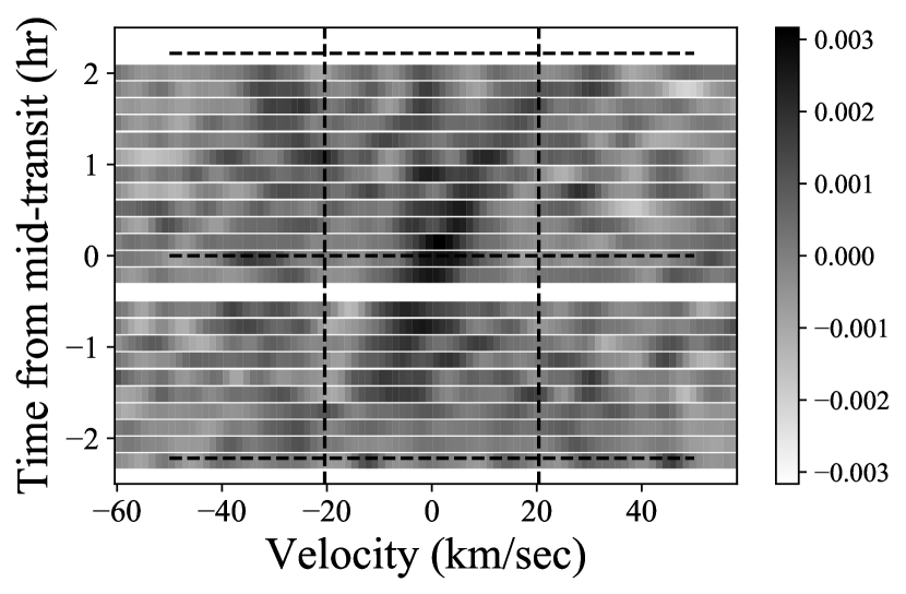
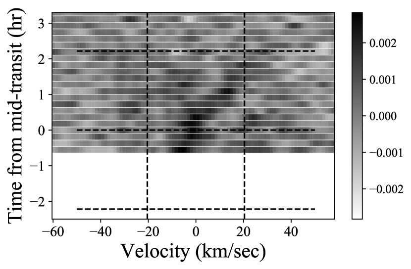
Figure 5: Spectroscopic transits of MASCARA-3 observed on the night of May 29, 2018 (left), and November 28, 2018 (right). Both plots show the observed CCFs, with the subtraction of the mean out-of-transit CCF obtained from the second night. Before subtraction, these CCFs were scaled and offset from their model counterpart in intensity (all CCFs) and scaled in velocity space (in-transit CCFs) in order to account for uneven normalization due to differences in flux levels and PSF changes. The vertical dashed lines mark the best-fit value of the $v\sin i_{\star}$ from the BF analysis, and the horizontal dashed lines mark the best-fit value for the transit ingress, mid-transit time, and egress.

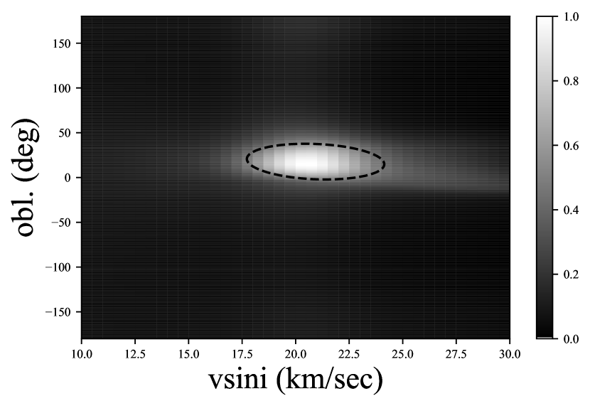
Figure 6: Enhancement ($v\sin i_{\star}$, $\lambda$) grid for the best-fit value of $b$ together with the best-fit $1\sigma$ 2D Gaussian model (dashed). For each ($v\sin i_{\star}$, $\lambda$, $b$) triple the grid values were constructed by shifting the model and shadow bump a corresponding amount, such that the model shadow bump is centered at zero. This was followed by collapsing the shifted data shadow in intensity space. The contour signal at a specific ($v\sin i_{\star}$, $\lambda$, $b$) value is then the resulting value of the collapsed shifted data shadow at a velocity of zero.

4.3 The RV-RM effect

To obtain a better constraint on the obliquity than what was possible from the Doppler shadow, we examined the possibility of extracting the RVs from the spectroscopic transit observations. Although we obtained large errors due to using ThAr during transit instead of an iodine cell, and although the RV errors are usually too high for this approach for fast-rotating stars, we were able to achieve an internal precision of 50 m s^-1. This precision, coupled with the small baseline and low number of data points, meant that obtaining $\lambda$ from the RVs was not possible for the transit night of November 28, 2018. However, it did prove sufficient for determining $\lambda$ from the observations of the full transit on the night of May 29, 2018.

The RV anomaly due to the RM-effect was modeled following Hirano et al. (2011). During the fitting routine, we varied $\lambda$, $v\sin i_{\star}$ , and $b$ as well an RV offset for the specific night $\gamma_{{\text{RM}}}$. We used the best-fitting values from the procedures described in Sects. 4.1 and 4.2 for the remaining parameters. We also applied a Gaussian prior of $v\sin i_{\star}=20.4\pm 0.4$ km s^-1 from the analysis of the stellar absorption and a Gaussian prior of $b=0.4\pm 0.1$ from the RV and light-curve analysis. We obtained $b=0.39\pm 0.08$, $v\sin i_{\star}=20.3\pm 0.4$ km s^-1 , and $\lambda=1.2^{+8.2}_{-7.4}$ deg, consistent with the results from Sect. 4.2.2, but with a much better constraint on the spin-orbit angle. Because out-of-transit data on the night of May 29, 2018, are scarce, leaving $K$ as an additional free parameter naturally made it poorly constrained, but it was still within 1$\sigma$ of the results from Sect. 4.1. The RV-RM data are given in Table 6 and are shown in Fig. 7 together with the best-fit model. The parameters are displayed in Table 4 and were obtained in the same way as in the previous sections.

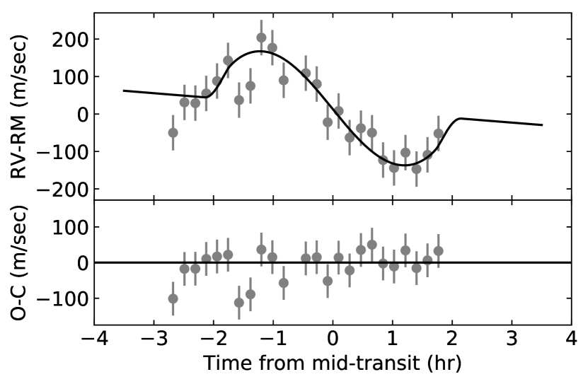
Figure 7: Radial velocities from the night of May 29, 2018, together with the best-fit model of the velocity anomaly. The uncertainties of $\sim 50$ m sec^-1 are higher than those of Fig. 3 because the calibrations during transit were performed with ThAr instead of the iodine cell.

5 Discussion and conclusions

From the joint photometry and RV analysis we obtain a planetary mass of $4.2\pm 0.2$ $M_{\text{Jup}}$ and a planetary radius of $1.36\pm 0.05$ $R_{\text{Jup}}$. The planet revolves around its host star in an almost circular orbit ($e=0.085^{+0.023}_{-0.022}$) every $5.55149\pm 0.00001$ days at a distance of $0.067\pm 0.002$ au. This means that MASCARA-3b is a hot Jupiter. With an incident flux of $F=(10.6\pm 0.9)\cdot 10^{8}$ erg s^-1 cm^-2 above the inflation threshold of $F=2\cdot 10^{8}$ erg s^-1 cm^-2 (Demory & Seager, 2011), the planet might be affected by inflation mechanisms although its mean density is higher than that of Jupiter.

It is still unclear whether hot Jupiters primarily originate from high-eccentricity migration (HEM) or disk migration (for a review, see Dawson & Johnson, 2018). The former process would lead to at least occasionally high obliquities, while the latter process would lead to low obliquities, assuming good alignment between stellar spin and angular momentum of the protoplanetary disks; but see also Bate (2018). However, the interpretation of hot Jupiter obliquities might be more complicated than originally thought because tidal interactions might have aligned the stellar spin and the orbital angular momentum in some of the systems, in particular in systems where the host stars have a convective envelope, which leads to fast alignment of the orbital spin of the planets with the stellar rotation (Winn et al. (2010); Albrecht et al. (2012)).

With an effective temperature of $T_{\text{eff},\star}=6415\pm 110$ K, MASCARA-3 has a relatively slow alignment timescale for a hot Jupiter of its mass and distance. It is also interesting to note that the orbital eccentricity suggests a near circular orbit. MASCARA-3 b appears to belong to a dynamically cold population consistent with an arrival at its current orbit through disk migration instead of HEM. However, we did find a long-term RV trend of $61\pm 19$ m s${}^{-}1$ yr${}^{-}1$ that might indicate the presence of a third body in the system. This body might have initiated HEM migrations through a scatter event or secular dynamics, such as Kozai-Lidov cycles.

While finalizing the manuscript, we learned of another paper reporting the discovery of this planet-star system that was published by the KELT team. Although no observations or analyses were shared, the planet and system parameters from each group agree for the most part. The only greater difference is the RV semi-amplitude, and thereby the derived planetary mass.

Appendix A Additional material

Table 5: Radial velocities at times out of transit for MASCARA-3 using the SONG telescope. We list the barycentric time of mid-exposure and the RVs corrected for barycentric motion. All spectra were taken with the iodine cell as reference. Although the individual uncertainties have some dependence on the flux level (which is near $30$ m sec^-1 at the highest and $60$ m sec^-1 at the lowest flux level), the overall instrumental uncertainty ($\sigma_{\text{RV}}$) is estimated to be $\sim 40$ m sec^-1. To account for the possibility of underestimating this error, we introduced an additional jitter term during the fitting procedure (see Table 4).

Time (BJD)	RV+6,000 (m s-1)
2458223.357685	613.1
2458224.382018	183.3
2458225.434460	67.3
2458233.607846	704.9
2458234.418452	770.2
2458235.720058	234.6
2458236.641036	32.2
2458237.678446	153.1
2458238.692052	603.9
2458241.674223	-70.7
2458243.368995	265.3
2458245.410918	805.6
2458246.571993	240.1
2458247.398019	-31.2
2458248.368253	82.6
2458249.365280	470.8
2458250.368275	844.0
2458250.681785	837.2
2458251.366037	687.0
2458251.666389	485.7
2458252.366480	192.9
2458253.365122	120.4
2458254.365100	237.8
2458255.374490	605.4
2458256.384282	796.1
2458257.382395	330.0
2458259.383303	18.0
2458263.567251	154.9
2458265.589542	291.4
2458267.372280	829.5
2458268.609046	306.4
2458270.572919	5.0
2458274.379165	192.8
2458280.423224	17.1
2458283.600292	812.6
2458418.763646	161.4
2458426.556824	222.3
2458434.627715	639.1
2458439.611331	713.9
2458448.692687	285.5
2458449.708606	658.2
2458450.690659	709.9
2458453.742034	106.8
2458454.745732	493.1
2458586.621310	20.0
2458594.703421	710.9
2458598.446201	150.2
2458600.395783	819.7
2458602.394577	19.7
2458604.398027	462.9
2458606.403578	680.6
2458608.402462	-36.2
2458610.402961	656.7
2458612.656473	323.0
2458614.640588	99.4
2458616.679269	892.4
2458621.434468	611.2
2458623.623973	586.7
2458625.668018	199.2
2458627.634024	974.2
2458629.638527	312.8
2458631.621685	345.4
2458633.654485	949.8
2458638.605001	913.8
2458643.571329	579.7

Table 6: Radial velocities during transit on the night of May 29, 2018, for MASCARA-3 using the SONG telescope. We list the barycentric time of mid-exposure and the RVs corrected for barycentric motion. All spectra were taken with the ThAr cell as reference, causing the uncertainties to be larger than the RVs reported in Table 5, in addition to a different RV offset. The instrumental uncertainty ($\sigma_{\text{RVRM}}$) is estimated to be $50$ m sec^-1.

Time (BJD)	RV${}_{\text{RM}}$+15,200 (m s-1)
2458268.353392	-14.0
2458268.361322	67.0
2458268.368937	65.0
2458268.376572	91.0
2458268.384095	124.0
2458268.391748	179.0
2458268.399454	73.0
2458268.407431	111.0
2458268.415063	240.0
2458268.422695	213.0
2458268.430603	126.0
2458268.446077	145.0
2458268.453711	116.0
2458268.461345	14.0
2458268.468981	44.0
2458268.476690	-27.0
2458268.484558	-2.0
2458268.492292	-14.0
2458268.500027	-87.0
2458268.507691	-108.0
2458268.515674	-67.0
2458268.523373	-111.0
2458268.531075	-73.0
2458268.538705	-16.0