Online Learning and Planning in Partially Observable Domains without Prior Knowledge

Supplementary Material: Online Learning and Planning in Partially Observable Domains without Prior Knowledge

Abstract

How an agent can act optimally in stochastic, partially observable domains is a challenge problem, the standard approach to address this issue is to learn the domain model firstly and then based on the learned model to find the (near) optimal policy. However, offline learning the model often needs to store the entire training data and cannot utilize the data generated in the planning phase. Furthermore, current research usually assumes the learned model is accurate or presupposes knowledge of the nature of the unobservable part of the world. In this paper, for systems with discrete settings, with the benefits of Predictive State Representations (PSRs), a model-based planning approach is proposed where the learning and planning phases can both be executed online and no prior knowledge of the underlying system is required. Experimental results show compared to the state-of-the-art approaches, our algorithm achieved a high level of performance with no prior knowledge provided, along with theoretical advantages of PSRs. Source code is available at https://github.com/DMU-XMU/PSR-MCTS-Online.

1 Introduction

One commonly used technique for agents operating in stochastic and partially observable domains is to learn or construct an offline model of the underlying system firstly, e.g., Partially Observable Markov Decision Processes (POMDPs) (Kaelbling et al., 1998) or Predictive State Representations (PSRs) (Littman et al., 2001; Hefny et al., 2018), then the obtained model can be used for finding the optimal policy. Although POMDPs provide a general framework for modelling and planning in partially observable and stochastic domains, they rely heavily on a prior known and accurate model of the underlying environment (Ross et al., 2008; Silver & Veness, 2010). While recent research showed the successful offline PSR-based learning and planning from scratch, offline learning a model needs to store the entire training data set and the model parameters in memory at once and the data generated during the planning phase is not utilized (Liu & Zheng, 2019).

Recently, with the successful applications of online and sample-based Monte-Carlo tree search (MCTS) techniques, e.g, AlphaGo (Silver et al., 2016), the BA-POMCP (Bayes-Adaptive Partially Observable Monte-Carlo Planning) algorithm (Katt et al., 2017, 2018), where the BA-POMDP framework (Ross et al., 2011) is combined with the MCTS approach, tries to deal with the problem of planning under model uncertainty in larger-scale systems. Unfortunately, the casting of the original problem into an POMDP usually leads to a significant complexity increase (with intractable large number of possible model states and parameters) and make it even harder to be solved, also, as is well-known, to find an (approximate) optimal solution to an POMDP problem in larger-scale systems is very difficult. Moreover, to guarantee the performance of the POMDP-based approaches, strong prior domain knowledge of the underlying system should be known in advance.

Unlike the latent-state based approaches, e.g., POMDPs, PSRs work only with the observable quantities, which leads to easier learning of a more expressive model, and more importantly, allows the learning of the model from scratch with no prior knowledge required (Littman et al., 2001; Liu et al., 2015, 2016; Hamilton et al., 2014). In the work of (Liu & Zheng, 2019), an offline PSR model is firstly learned using training data, then the learned model is combined with MCTS for finding optimal policies. Although compared to the BA-POMDP based approaches, the offline PSR model-based planning approach has achieved significantly better performance and can plan from scratch (Liu & Zheng, 2019), as mentioned, offline learning the model often needs to store the entire training data and cannot utilize the data generated in the planning phase, moreover, for the offline learning of the PSR model, $|A|\times|O|$ matrices $P_{T,ao,H}$ are needed to be stored and computed, where $|A|$ the number of actions, $|O|$ the number of observations, $H$ the possible histories and $T$ the possible tests respectively (See Background for details of history and test). For large scale systems, the storing and calculating such large number of large matrices are expensive and time-consuming (Boots & Gordon, 2011). Recent research has shown the successful online learning of the PSR model, where the model can be updated incrementally when new training data arrives, and the storing and manipulation of $P_{T,ao,H}$ is not required (Boots & Gordon, 2011; Hamilton et al., 2014). Also, the space complexity of the learned model is independent of the number of training examples and its time complexity is linear in the number of training examples (Boots & Gordon, 2011).

In this paper, as an alternative and improvement to the offline technique, we introduce an online learning and planning approach for agents operating in partially observable domains with discrete settings, where the model can be learned online and the planning can be started from scratch with no prior knowledge of the domain provided. At each step, the PSR model is online updated and used as the simulator for the computation of the local policies of MCTS. Experiments on some benchmark problems show that with no prior knowledge provided in both cases, our approach performs significantly better than the state-of-the-art BA-POMDP-based algorithms. The effectiveness and scalability of our approach are also demonstrated by scaling to learn and plan in larger-scale systems, the RockSample problem (Smith & Simmons, 2004; Ross et al., 2011), which is infeasible for the BA-POMDP-based approaches. We further compared our online technique to the offline PSR-based approaches (Liu & Zheng, 2019), and experiments show the performance of the online approach is still competitive while requiring less computation and storage resources. As also can be seen from the experiments, with the increase complex of the underlying system, the online approach outperforms the offline techniques while reserving the theoretical advantages of the PSR-related approaches.

2 Background

PSRs offer a powerful framework for modelling partially observable systems by representing states using completely observable events (Littman et al., 2001). For discrete systems with finite set of observations $O=\{o^{1},o^{2},\cdots,o^{|O|}\}$ and actions $A=\{a^{1},a^{2},\cdots,a^{|A|}\}$, at time $\tau$, the observable state representation of the system is a prediction vector of some tests conditioned on current history, where a test is a sequence of action-observation pairs that starts from time $\tau+1$, a history at $\tau$ is a sequence of action-observation pairs that starts from the beginning of time and ends at time $\tau$, and the prediction of a length-$m$ test $t$ at history $h$ is defined as $p(t|h)=p(ht)/p(h)=\prod^{m}_{i=1}Pr(o_{i}|ha_{1}o_{1}\cdots a_{i})$ (Singh et al., 2004; Liu & Zheng, 2019).

The underlying dynamical system can be described by a special bi-infinite matrix, called the Hankel matrix (Balle et al., 2014), where the rows and columns correspond to the possible tests $\mathcal{T}$ and histories $\mathcal{H}$ respectively, the entries of the matrix are defined as $P_{t,h}=p(ht)$ for any $t\in\mathcal{T}$ and $h\in\mathcal{H}$, where $ht$ is the concatenation of $h$ and $t$ (Boots et al., 2011). The rank of the Hankel matrix is called the linear dimension of the system (Singh et al., 2004; Huang et al., 2018). Then a PSR of a system with linear dimension $k$ can be parameterized by a reference condition state vector $b_{*}=b(\epsilon)\in\mathbb{R}^{k}$, an update matrix $B_{ao}\in\mathbb{R}^{k\times k}$ for each $a\in A$ and $o\in O$, and a normalization vector $b_{\infty}\in\mathbb{R}^{k}$, where $\epsilon$ is the empty history and $b_{\infty}^{T}B_{ao}=1^{T}$ (Hsu et al., 2012; Boots et al., 2011). Using these parameters, the PSR state at next time step $b(hao)$ can be updated from $b(h)$ as follows (Boots et al., 2011):

$$b(hao)=\frac{B_{ao}b(h)}{b_{\infty}^{T}B_{ao}b(h)}.$$ (1)

Also, the probability of observing the sequence $a_{1}o_{1}a_{2}o_{2}\cdots a_{n}o_{n}$ in the next $n$ time steps can be predicted by (Boots et al., 2011; Liu & Zheng, 2019):

$$Pr[o_{1:t}||a_{1:t}]=b_{\infty}^{T}B_{a_{n}o_{n}}\cdots B_{a_{2}o_{2}}B_{a_{1}o_{1}}b_{*}.$$ (2)

Many approaches have been proposed for the offline PSR model learning(Boots et al., 2011; Liu et al., 2015, 2016), and recently, some online spectral learning approaches of the PSR model have been developed (Boots & Gordon, 2011; Hamilton et al., 2014). The details of those approaches are showed in Appendix A.

It is shown the learned model is consistent with the true model under some conditions (Hamilton et al., 2014; Liu & Zheng, 2019). Also note rather than offline storing and computing $|A|\times|O|$ matrices $P_{T,ao,H}$ for the offline learning of the PSR model (Liu & Zheng, 2019), for the online learning of the PSR model, these matrices are not needed (Boots & Gordon, 2011; Hamilton et al., 2014).

3 Online Learning and Planning without Prior Knowledge

For online planning in partially observable and stochastic domains with discrete settings, the most practical solution is to extend MCTS to the model of the underlying environment, where MCTS iteratively builds a search tree with node $T(h)$ that contains $N(h)$, $N(h,a)$, and $V(h,a)$ to combine Monte-Carlo simulation with game tree search (Gelly et al., 2012; Silver & Veness, 2010). At each decision step, besides for being used for state updating, the model is used to generate simulated experiments for MCTS to construct a lookahead search tree for forming a local approximation to the optimal value function, where each simulation contains two stages: a tree policy and a rollout policy (Silver & Veness, 2010; Katt et al., 2017). While current research shows the success of the model-based MCTS on some benchmark problems, either the used model is assumed to be known a prior and accurate (Silver & Veness, 2010) or some strong assumptions on the model is made to guarantee the planning performance, e.g, a nearly correct initial model (Ross et al., 2011; Katt et al., 2017, 2018) or the model can be only learned offline (Liu & Zheng, 2019).

Algorithm 1 PSR-MCTS-Online($Z$, $num\_episodes$)

  $//$Get  initial   model  parameters

  ${\textstyle\hat{\sum}_{\mathcal{H}}}$, ${\textstyle\hat{\sum}_{\mathcal{T,H}}}$ $\leftarrow$ Matrices estimated by initial training data $Z$ in an online mannner

  $(\hat{U},\hat{S},\hat{V})=SVD(\textstyle\hat{\sum}_{\mathcal{T,H}})$

  $\hat{b}_{1}$, $\hat{b}_{\infty}^{T}$, $\hat{B}_{ao}$ $\leftarrow$ Model parameters calculated using $(\hat{U},\hat{S},\hat{V})$

  for $i\leftarrow 1$ to $n\_episodes$ do

     $//$Get new training data $Z^{{}^{\prime}}$ and updated model  parameters

     $Z^{{}^{\prime}}$=PSR-MCTS($h$)

     ${\textstyle\hat{\sum}_{\mathcal{H}}}$, ${\textstyle\hat{\sum}_{\mathcal{T,H}}}$ $\leftarrow$ Updated model parameters with new arriving data $Z^{{}^{\prime}}$

     $\hat{U},\hat{S},\hat{V}$ $\leftarrow$ Execute SVD on updated ${\textstyle\hat{\sum}_{\mathcal{T,H}}}$ or using the methods of (Brand, 2002)

     $\hat{b}_{1}$, $\hat{B}_{ao}$, $\hat{b}_{\infty}^{T}$, $\leftarrow$ Model parameters re-computed in an online manner

  end for

Algorithm 2 PSR-MCTS($h$)

  $h\leftarrow()$

  $b(h)\leftarrow\hat{b}_{1}$

  repeat

     $//$Select action according to $\varepsilon$-greedy policy

     $a\leftarrow$ $\left\{\begin{array}[]{lc}1-\varepsilon&\ \ Act-Search(b\left(h\right),n\_sims,h)\\ \frac{\varepsilon}{|A|-1}&for\;all\;other\;|A|-1\;actions\;a\end{array}\right.$

     

     EXECUTE $a$

     $o\leftarrow$ observation received from the world

     $//$Update belief state based on received observations

     $b(hao)=\frac{\hat{B}_{ao}b(h)}{\hat{b}_{\infty}^{T}\hat{B}_{ao}b(h)}$

     $h\leftarrow hao$

  until the end of a plan

  return $h$

In this section, we show how the online-learned PSR model can be combined with MCTS. As mentioned, PSRs use completely observable quantities for the state representation and the spectral learned PSR model is consistent with the true model, moreover no prior knowledge is required to learn a PSR model (Hamilton et al., 2014). In our approach, with the benefits of PSRs and its online learning approach, the PSR model is firstly learned and updated in an online manner (Algorithm 3). Then at each decision step, as commonly used in the literature (Silver & Veness, 2010; Katt et al., 2017; Liu & Zheng, 2019), the (learned) model can be straightforwardly used to generate the simulated experiments for MCTS to find the good local policy (Note that functions Act-Search and Simulate are the same as in the work of (Liu & Zheng, 2019), we refer the readers to see it or Appendix B for the detail). After the found action is executed and a real observation is received, the model and the next state representation is updated. For the MCTS process, in the simulation, at each time step, after an action is selected, an observation is sampled according to $Pr[o||ha]=\hat{b}_{\infty}^{T}\hat{B}_{ao}b(h)$ by following Equ.2.

Then the state in the simulation is also updated. Note that in the POMDP-based MCTS approaches, such state update and observation sampling are also needed (Silver & Veness, 2010; Katt et al., 2017, 2018), and as shown in the work of (Liu & Zheng, 2019), when compared to the POMDP-based approaches, the state representation of the PSR-based approach is more compact and the computation of the next observation is more efficient.

In the partially observable environments, as we cannot know exactly some states, it is difficult to determine the rewards related to these states. In our approach, as used in the offline technique (Liu & Zheng, 2019), we directly treat some rewards as observations, e.g., the goal related rewards, and these observations (rewards) are used in the online model learning. In the simulation, when the sampled observation $o$ is the reward that indicates the end of a process, the simulation ends. Otherwise, the simulation ends with some pre-defined conditions. Note that some state-independent rewards, such as the rewards received at every time step or action-only-dependent rewards in some domains, are not treated as observations and not used for the model learning (Liu & Zheng, 2019). After a real observation $o$ is received from the world, $h\leftarrow hao$, $b(h)$ is updated according to Equ. 1, and the node $T(h)$ becomes the root of the new search tree.

4 Experimental Results

4.1 Experimental setting

           Tiger                             POSyadmin                        RockSample(5,5)                      RockSample(5,7)

($a$)

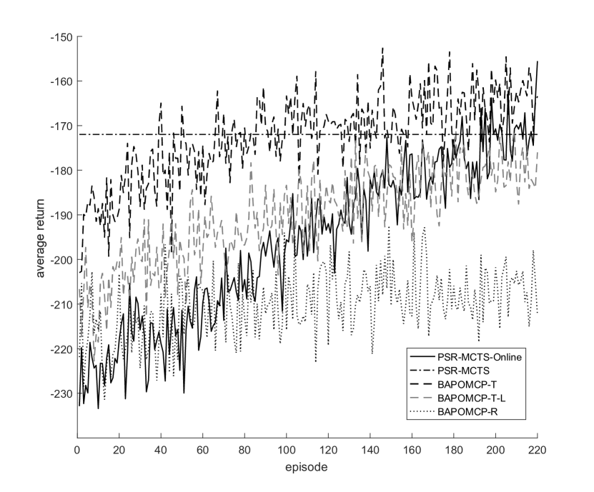
($b$)

($c$)

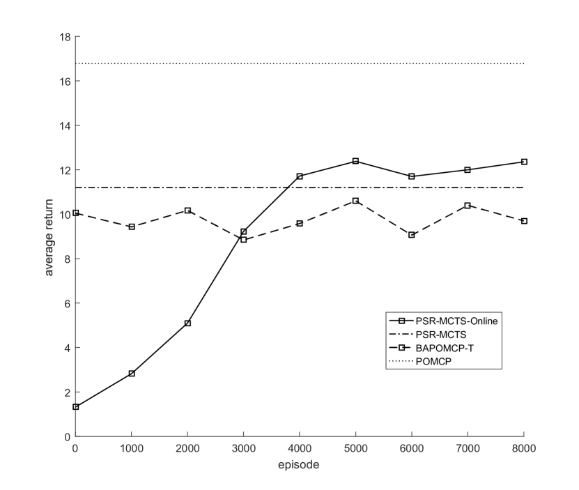
($d$)

Figure 1: Average return for different algorithms in different domains

To evaluate our proposed approach, we first executed our algorithm on Tiger and POSyadmin, the two problems used to test the state-of-the-art BA-POMCP approach (Katt et al., 2017, 2018). Then we extend our approach to RockSample(5,5) and RockSample(5,7) (Smith & Simmons, 2004; Ross et al., 2011), both of which are too complex for the BA-POMDP based approaches.

The details of the experimental settings in our approach are showed in Appendix C.

4.2 Evaluated methods

As mentioned, the performance of the BA-POMDPs based approaches rely heavily on knowing the knowledge of the underlying system (Katt et al., 2017, 2018), for example, in the work of (Katt et al., 2017), for Tiger, the transition model is assumed to be correct and the initial observation function is assumed to be nearly correct; for POSyadmin, the observation function is assumed known a prior, and the initial transition function is assumed to be nearly correct; for RockSample, in the work of (Ross et al., 2011), the transition model is assumed to be correct and the initial observation function is assumed to be nearly correct.

To evaluate our method, for the first two problems, we firstly compared our approach to the BA-POMCP method under the same conditions (BAPOMCP-R), that is, no prior knowledge is provided to the BA-POMCP approach, then our approach was compared to the BA-POMCP approach with the nearly correct initial models (BAPOMCP-T) as mentioned previously. For POSyadmin, we also compared our approach to the BA-POMCP approach with the less accurate initial model (BAPOMCP-T-L), where the true probabilities of transition function are either subtracted or added by $0.4$, and for probabilities fall below $0$, they are set to $0.001$. Then, each Dirichlet distribution is normalized with the counts summing to $20$. For the RockSample problem, our approach was compared to the BA-POMCP approach with the nearly correct initial models (BAPOMCP-T). We also show the result of the POMCP approach (Silver & Veness, 2010) where the accurate models of the underlying systems are used. To further verify the performance of the online approach, we also compared with the offline PSR model learning-based approach (PSR-MCTS) (Liu & Zheng, 2019) where the PSR model is firstly learned offline and then combined with MCTS for planning.

4.3 Performance evaluation

Figure 1:($a$) plots the average return over 10000 runs with 10000 simulations at each decision step of MCTS on Tiger. For Tiger, for the BAPOMCP-R approach, nearly no improvement has been achieved with the increase of episodes and for the BAPOMCP-T approach, with the increase of the episodes, the performance becomes stable. For our PSR-MCTS-Online approach, with the increase of the learning episodes, our approach performs significantly better than the BAPOMCP-R approach. And finally, our approach achieves the same performance with the BAPOMCP-T approach, which has strong prior knowledge provided.

Experimental results for four approaches on the (3-computer) POSysadmin problem are shown in Figure 1:($b$), where 100 simulations per step were used. For the BAPOMCP-T and BAPOMCP-T-L approach, the results tend to be stable after 150 episodes, and for the BAPOMCP-R approach, nearly no improvement has been achieved with the increase of the episodes. Our PSR-MCTS-Online approach still performs significantly better than the BAPOMCP-R approach and finally achieves nearly the same performance of the BAPOMCP-T approach. While for the BAPOMCP-T-L approach, after less than $150$ episodes, our approach has a better performance.

Figure 1:($c$) and Figure 1:($d$) plot the average return over 1000 runs with 1000 simulations on RockSample(5,5) and RockSample(5,7). For such scale systems, the state size of the BA-POMDP model is intractable large with the increase of the time step, and we may not be able even to store and initialize the state transaction matrices. For the convenience of the comparison, as used in the work of (Ross et al., 2011), only the dynamics related to the check action were modeled via the BA-POMDP approach, for the others, the black box simulation of the exact model was used to generate the simulated experiments and for state representation and updating (BAPOMCP-T). Even under such conditions, the PSR-MCTS-Online method without no prior knowledge provided finally still achieved the nearly same or better performance with the BAPOMDP-T approach. Even compared to the POMCP method where the underlying model is accurate, the performance of our approach is still competitive.

When compared with the offline based approach (Liu & Zheng, 2019), while without requiring the storing and computation of the $|A|\times|O|$ $P_{T,ao,H}$ matrices, for Tiger, POSysadmin and RockSample(5,5), the online approach eventually achieved the same performance of the offline method, and with the increase of the complexity of the underlying domain, for RockSample(5,7), with the increase of the episodes, the online approach outperforms the offline technique.

5 Conclusion

In this paper, we presented PSR-MCTS-Online, a method that can simultaneously learn and plan in an online manner while not requiring any prior knowledge provided. Experimental results show the effectiveness and scalability of the proposed method with the theoretical advantages of the PSR-related approaches. When compared to the offline approach, the effectiveness of the online approach is also demonstrated while requiring less computation and storage resource.

A Online Spectral Algorithm

Given any length training trajectory $z$ of action-observation pairs in a batch of training trajectories $Z$, three indicator functions, $\mathbb{I}_{h_{j}(z)}$, $\mathbb{I}_{h_{j},t_{i},(z)}$ and $\mathbb{I}_{h_{j},ao,t_{i},(z)}$ for $z\in Z$, are firstly defined, where $\mathbb{I}_{h_{j}(z)}$ takes a value of 1 if the action-observation pairs in $z$ correspond to $h_{j}$, $\mathbb{I}_{h_{j},t_{i},(z)}$ takes a value of 1 if $z$ can be partitioned to make that there are $\left|h_{j}\right|$ action-observation pairs corresponding to those in $h_{j}\in\mathcal{H}$ and the next $\left|t_{i}\right|$ pairs correspond to those in $t_{i}\in\mathcal{T}$, and $\mathbb{I}_{h_{j},ao,t_{i},(z)}$ takes a value of 1 if $z$ can be partitioned to make that there are $\left|h_{j}\right|+1$ action-observation pairs corresponding to $h_{j}$ appended with a particular $ao\in A\times O$ and the next $\left|t_{i}\right|$ pairs correspond to those in $t_{i}\in\mathcal{T}$ respectively (Hamilton et al., 2014). Then the following matrices can be estimated:

$${\textstyle\hat{\sum}_{\mathcal{H}}}=\sum_{z\in Z}\mathbb{I}_{h_{j}(z)}\\$$ (3)

$${\textstyle\hat{\sum}_{\mathcal{T,H}}}=\sum_{z\in Z}\;\sum_{t_{i},h_{j}\in\mathcal{T}\times\mathcal{H}}\mathbb{I}_{h_{j},t_{i},(z)}\\$$ (4)

Next, an SVD is executed on matrix $\textstyle\hat{\sum}_{\mathcal{T,H}}$ to obtain $(\hat{U},\hat{S},\hat{V})=SVD(\textstyle\hat{\sum}_{\mathcal{T,H}})$, then the corresponding model parameters are as follows:

$$\hat{b}_{1}=\hat{S}\hat{V}^{T}e$$ (5)

$$\hat{b}_{\infty}^{T}=\hat{\textstyle\sum}_{H}^{T}\hat{V}\hat{S}^{-1}$$ (6)

and for each $ao\in A\times O$:

$$\hat{B}_{ao}=\sum_{z\in Z}\;\sum_{t_{i},h_{j}\in\mathcal{T}\times\mathcal{H}}\mathbb{I}_{h_{j},ao,t_{i}}\left(z\right)\left[\hat{U}^{T}\left(t_{i}\right)\hat{S}^{-1}\hat{V}^{T}\left(h_{j}\right)\right]$$ (7)

where $e$ is a vector such that $e=(1,0,0,\cdots,0)^{T}$. This specification of $e$ assumes all $z\in Z$ are starting from a unique start state. If this is not the case, then $e$ is set such that $e=(1,1,1,\cdots,1)^{T}$. In this latter scenario, rather than learning $\hat{b}_{1}$ exactly, $\hat{b}_{*}$ is learned, which is an arbitrary feasible state as the start state (Hamilton et al., 2014). $\hat{U}^{T}\left(t_{i}\right)$ is the $t_{i}^{th}$ row of matrix $\hat{U}^{T}$, and $\hat{S}^{-1}\hat{V}^{T}$$\left(h_{j}\right)$ is the $h_{j}^{th}$ column of matrix $\hat{S}^{-1}\hat{V}^{T}$ (Boots et al., 2011; Hamilton et al., 2014).

With the arriving of new training data $Z^{{}^{\prime}}$, the model parameters can be incrementally updated in an online manner that ${\textstyle\hat{\sum}_{\mathcal{H}}}$ and ${\textstyle\hat{\sum}_{\mathcal{T,H}}}$ are updated accordingly by using Equ. 3 and 4, then a new $(\hat{U}_{new},\hat{S}_{new},\hat{V}_{new})$ can be obtained by executing SVD on the updated ${\textstyle\hat{\sum}_{\mathcal{T,H}}}$. Note that in the case of a large amount of training data, the method proposed in the work of (Brand, 2002) can be used for the updating of ${\textstyle\hat{\sum}_{\mathcal{T,H}}}$ for improving the efficiency of the calculation. Accordingly, parameters $\hat{b}_{1}$ and $\hat{b}_{\infty}$ can be re-computed by using Equ. 5 and Equ. 6, $\hat{B}_{ao}$ can be updated as follows with $Cnt_{ao}=\sum_{z\in Z}\;\sum_{t_{i},h_{j}\in\mathcal{T}\times\mathcal{H}}\mathbb{I}_{h_{j},ao,t_{i}}\left(z\right)$:

$$\begin{split}&\hat{B}_{ao}=\\ &\sum_{t_{i},h_{j}\in\mathcal{T}\times\mathcal{H}}Cn{t_{ao}}\left[t_{i},h_{j}\right]{\hat{U}^{T}}_{new}\left(t_{i}\right)\hat{S}^{-1}_{new}{\hat{V}^{T}}_{new}\left(h_{j}\right)\end{split}$$ (8)

When the total amount of training data is large, $\hat{B}_{ao}$ can also be updated directly as follows (Hamilton et al., 2014):

$$\begin{split}&\hat{B}_{ao}=\\ &\sum_{z\in Z^{{}^{\prime}}}\;\sum_{t_{i},h_{j}\in\mathcal{T}\times\mathcal{H}}\mathbb{I}_{h_{j},ao,t_{i}}\left(z\right)\left[\hat{U}_{new}^{T}\left(t_{i}\right){\hat{S}_{new}}^{-1}\hat{V}_{new}^{T}\left(h_{j}\right)\right]+\\ &\hat{U}_{new}^{T}{\hat{U}}_{old}\hat{B}_{ao}^{old}{\hat{S}}_{old}\hat{V}_{old}^{T}{\hat{V}}_{new}\hat{S}_{new}^{-1}\end{split}$$ (9)

It is shown the learned model is consistent with the true model under some conditions (Hamilton et al., 2014; Liu & Zheng, 2019). Also note that rather than offline storing and computing $|A|\times|O|$ matrices $P_{T,ao,H}$ for the offline learning of the PSR model as mentioned previously, for the online learning of the PSR model, these matrices are not needed.

B PSR-MCTS-Online Algorithm

In the algorithms, $reward(ao)$ is the reward that is not treated as observation, $\gamma$ is a discounted factor specified by the environment, $n\_sims$ is the number of simulations used for MCTS to find the executed action at each step, $max\_dep$ and $IsTerminal(h)$ are some predefined conditions for the termination (Note that Functions Act-Search, Simulate and RollOut are the same as in the work of (Liu & Zheng, 2019)).

Algorithm 3 PSR-MCTS-Online($Z$, $num\_episodes$)

  $//$Get  initial   model  parameters

  ${\textstyle\hat{\sum}_{\mathcal{H}}}$, ${\textstyle\hat{\sum}_{\mathcal{T,H}}}$ $\leftarrow$ Estimated by initial training data $Z$ using Equ. 3                           and Equ. 4

  $(\hat{U},\hat{S},\hat{V})=SVD(\textstyle\hat{\sum}_{\mathcal{T,H}})$

  $\hat{b}_{1}$, $\hat{b}_{\infty}^{T}$, $\hat{B}_{ao}$ $\leftarrow$ Calculated by Equ. 5, Equ. 6 and Equ. 7

  for $i\leftarrow 1$ to $n\_episodes$ do

     $//$Get new training data $Z^{{}^{\prime}}$ and updated model  parameters

     $Z^{{}^{\prime}}$=PSR-MCTS($h$)

     ${\textstyle\hat{\sum}_{\mathcal{H}}}$, ${\textstyle\hat{\sum}_{\mathcal{T,H}}}$ $\leftarrow$ Updated by Equ. 3 and Equ. 4 with $Z^{{}^{\prime}}$

     $\hat{U},\hat{S},\hat{V}$ $\leftarrow$ Execute SVD on updated ${\textstyle\hat{\sum}_{\mathcal{T,H}}}$ or using the methods of (Brand, 2002)

     $\hat{b}_{1}$, $\hat{b}_{\infty}^{T}$, $\leftarrow$ Re-computed by using Equ. 5, Equ. 6

     $\hat{B}_{ao}$ $\leftarrow$ Updated by using Equ. 8 or Equ. 9

  end for

Algorithm 4 PSR-MCTS($h$)

  $h\leftarrow()$

  $b(h)\leftarrow\hat{b}_{1}$

  repeat

     $//$Select action according to $\varepsilon$-greedy policy

     $a\leftarrow$ $\left\{\begin{array}[]{lc}1-\varepsilon&\ \ Act-Search(b\left(h\right),n\_sims,h)\\ \frac{\varepsilon}{|A|-1}&for\;all\;other\;|A|-1\;actions\;a\end{array}\right.$

     

     EXECUTE $a$

     $o\leftarrow$ observation received from the world

     $//$Update belief state based on received observations

     $b(hao)=\frac{\hat{B}_{ao}b(h)}{\hat{b}_{\infty}^{T}\hat{B}_{ao}b(h)}$

     $h\leftarrow hao$

  until the end of a plan

  return $h$

Algorithm 5 Act-Search($b(h)$,$n\_sims$,$h$)

  $h_{0}\leftarrow h$

  $\bar{b}(h_{0})\leftarrow Copy(b(h))$

  for $i\leftarrow 1$ to $n\_sims$ do

     $Simulate(\bar{b}(h_{0}),0,h_{0})$

  end for

  $a\leftarrow GreedyActionSelection(h_{0})$

  return $a$

Algorithm 6 Simulate($b(h),depth,h$)

  if $depth==max\_dep\|IsTerminal(h)$ then

     return $0$

  end if

  $//$Select action according to the UCT algorithm (Kocsis & Szepesvári, 2006)

  $a\leftarrow$ UCBACTIONSELECTION($h$)

  $//$Obtain observation using the PSR method

  $o\leftarrow$ sampled according to $Pr[o||ha]=\hat{b}_{\infty}^{T}\hat{B}_{ao}b(h)$

  if $o$ corresponds to some reward then

     $R\leftarrow reward(o)$

  else

     $R\leftarrow reward(ao)$

  end if

  $//$Update belief state

  $h^{\prime}\leftarrow hao$

  $b(h^{\prime})=\frac{\hat{B}_{ao}b(h)}{\hat{b}_{\infty}^{T}\hat{B}_{ao}b(h)}$

  if $h^{\prime}\in Tree$ then

     $r\leftarrow R+\gamma\cdot$Simulate($b(h^{\prime}),depth+1,h^{\prime}$)

  else

     ConstructNode($h^{\prime}$)

     $r\leftarrow R+\gamma\cdot$RollOut($b(h^{\prime}),depth+1,h^{\prime}$)

  end if

  $//$Update statistics. $N(h)$: number of times history $h$ has been visited. $V(h,a)$: value of $h$

  $N(h)\leftarrow N(h)+1$

  $N(h,a)\leftarrow N(h,a)+1$

  $V(h,a)\leftarrow V(h,a)+\frac{r-V(ha)}{N(ha)}$

  return $r$

Algorithm 7 RollOut($b(h),depth,h$)

  if $depth==max\_dep\|IsTerminal(h)$ then

     return $0$

  end if

  $//$Using the rollout policy (random policy) to select the action to perform

  $a\leftarrow\pi_{rollout}(h)$

  $//$Obtain observation using the PSR method

  $o\leftarrow$ sampled according to $Pr[o||ha]=\hat{b}_{\infty}^{T}\hat{B}_{ao}b(h)$

  if $o$ corresponds to some reward then

     $R\leftarrow reward(o)$

  else

     $R\leftarrow reward(ao)$

  end if

  $//$Update belief state

  $h^{\prime}\leftarrow hao$

  $b(h^{\prime})=\frac{\hat{B}_{ao}b(h)}{\hat{b}_{\infty}^{T}\hat{B}_{ao}b(h)}$

  $r\leftarrow R+\gamma\cdot$RollOut($b(h^{\prime}),depth+1,h^{\prime}$)

  return $r$

C Experimental setting

For POSyadmin, the agent acts as a system administrator to maintain a network of $n$ computers. The agent doesn’t know the state of any computer, and at each time step, any of the computers can ’fail’ with some probability $f$ (Katt et al., 2017). In the RockSample($n,k$) domain (Figure 2 and 3), a robot is on an $n\times n$ square board, with $k$ rocks on some of the cells. Each rock has an unknown binary quality (good or bad). The goal of the robot is to gather samples of the good rocks. The state of the robot is defined by the position of the robot on the board and the quality of all the rocks and there is an additional terminal state, reached when the robot moves into exit area, then with a $n\times n$ board and $k$ rocks, the number of states is $n^{2}2^{k}+1$ (Ross et al., 2011).

Figure 2: RockSample(5,5).

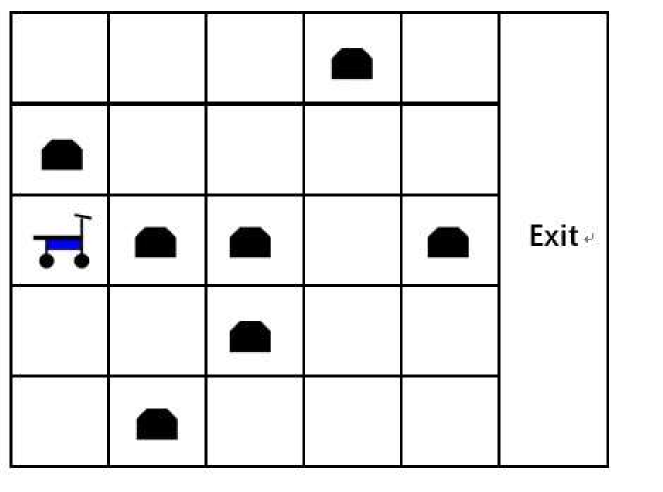
Figure 3: RockSample(5,7).

For Tiger, besides the two observations of the original domain, the reward 10 for opening the correct door and the penalty $-100$ for choosing the door with the tiger behind it are treated as observations. For POSyadmin, we added the rewards that indicate the whole status of the network as observations, which provides the information about how many computers have been failed at current step, but we still don’t know which computer has been failed, the same rewards were also used in the BA-POMCP based experiments. For RockSample, we treat the reward $10$ for sampling a good rock or moving into exit area and the penalty $-10$ for sampling a bad rock as observations. Also, as the PSR model is learned from scratch, the online learning and planning of our approach is divided into two phases. In the first phase, no model-based decision has been made, and the random policy is used to explore the environment to obtain an initial model. Then, while the model is still updated with the arriving of new training data, the $\varepsilon$-greedy policy is used in the decision process, where $\varepsilon$ will decrease to zero with the increase of the episodes.

The details of the experimental settings in our approach are as follows: For Tiger, the maximum length of $\mathcal{H}$ is set to $6$ and the maximum length of $\mathcal{T}$ is set to $2$; For POSyadmin, the maximum length of $\mathcal{H}$ is set to $12$ and the maximum length of $\mathcal{T}$ is set to $1$; For RockSample(5,5) and RockSample(5,7), the maximum length of $\mathcal{H}$ is set to $27$ and the maximum length of $\mathcal{T}$ is set to $2$. A random strategy is used in the first 20, 20, 40, and 1000 episodes for Tiger, POSyadmin, RockSample(5,5) and RockSample(5,7) respectively. For RockSample, the random policy is as follows: Each rock is checked twice at most; when the robot is in the cell of the rock, once the rock has been checked, the sample action will be performed; otherwise the sample action will be performed with a 50% probability. In all other cases, the robot randomly selects an action. For tiger, $\varepsilon$ decreases from $0.5$ to $0$ at a constant speed from the 21st episode to the 100th episode. For POSyadmin, $\varepsilon$ decreases from $0.85$ to $0$ at a constant speed from the 21st episode to the 200th episode. For RockSample(5,5), from the 41st episode to the 200th episode, $\varepsilon$ is initially set to 0.8, then at every 40 episodes $\varepsilon$ is reduced by 0.2. For RockSample(5,7), from the 1001st episode to the 5000th episode, $\varepsilon$ is initially set to 0.8, and at every 1000 episodes $\varepsilon$ is reduced by 0.2. Note that some different parameters have also been tested, and similar performance has been achieved for our approach.

D Related Works

POMDPs are a general solution for the modelling of controlled systems, however, it is known that learning offline POMDP models using some EM-like methods is very difficult and suffers from local minima, moreover, these approaches presuppose knowledge of the nature of the unobservable part of the world. As an alternative, PSRs provide a powerful framework by only using observable quantities. Much effort has been devoted to learning offline PSR models. In the work of Boots et al. (Boots et al., 2011), the offline PSR model is learned by using spectral approaches. Hamilton et al. (Hamilton et al., 2014) presented the compressed PSR (CPSR) models, and the technique learns approximate PSR models by exploiting a particularly sparse structure presented in some domains. The learned CPSR model is also combined with Fitted-Q for planning, but prior knowledge, e.g., domain knowledge, is still required. Hefny et al. (Hefny et al., 2018) proposed Recurrent Predictive State Policy (RPSP) networks, which consist of a recursive filter for the tracking of a belief about the state of the environment, and a reactive policy that directly maps beliefs to actions, to maximize the cumulative reward. In the work of (Liu & Zheng, 2019), an offline PSR model is firstly learned using training data, then the learned model is combined with MCTS for finding optimal policies. Although compared to the BA-POMDP based approaches, the offline PSR model-based planning approach has achieved significantly better better performance, offline learning the model often needs to store the entire training data and cannot utilize the data generated in the planning phase, moreover, for the offline learning of the PSR model, $|A|\times|O|$ matrices $P_{T,ao,H}$.

To alleviate the shortcoming of offline PSR model learning techniques that the entire training data is needed to store in memory at once, the online PSR model learning approach has been proposed in the work of (Boots & Gordon, 2011; Hamilton et al., 2014), where the model can be updated incrementally when new training data arrives, also, the learned model’s space complexity is independent of the number of training examples and its time complexity is linear in the number of training examples.

When the model of the underlying system is available, model-based planning approaches offer a principled framework for solving the problem of choosing optimal actions, however, most of the related methods assume an accurate model of the underlying system to be known a prior, which is usually unrealistic in real-world applications. The BA-POMDP approach tackles this problem by using a Bayesian approach to model the distribution of all possible models and allows the models to be learned during execution (Ross et al., 2011; Ghavamzadeh et al., 2015). Unfortunately, BA-POMDPs are limited to some trivial problems as the size of the state space over all possible models is too large to be tractable for non-trivial problems.

With the benefits of online and sample-based planning for solving larger problems (Kearns et al., 2002; Ross et al., 2008; Silver & Veness, 2010), some approaches have been proposed to solve the BA-POMDP model in an online manner. In the work of (Ross et al., 2011), an online POMDP solver is proposed by focusing on finding the optimal action to perform in the current belief of the agent. Katt et al. (Katt et al., 2017, 2018) extend the Monte-Carlo Tree Search method POMCP to BA-POMDPs, results in the state-of-the-art framework for learning and planning in BA-POMDPs. In the work of (Katt et al., 2018), a Factored Bayes-Adaptive POMDP model is introduced by exploiting the underlying structure of some specific domains. While these approaches show promising performance on some problems, like other Bayesian-based approaches in the literature, the performance is very dependent on the prior knowledge.

References

- Balle et al. (2014) Balle, B., Carreras, X., Luque, F. M., and Quattoni, A. Spectral learning of weighted automata. Machine Learning, 96(1-2):33–63, 2014.
- Boots & Gordon (2011) Boots, B. and Gordon, G. An online spectral learning algorithm for partially observable nonlinear dynamical systems. In Proceedings of the 25th National Conference on Artificial Intelligence (AAAI), 2011.
- Boots et al. (2011) Boots, B., Siddiqi, S., and Gordon, G. Closing the learning planning loop with predictive state representations. International Journal of Robotic Research, 30:954–956, 2011.
- Brand (2002) Brand, M. Incremental singular value decomposition of uncertain data with missing values. Computer Vision-ECCV 2002, 2350:707–720, 2002.
- Gelly et al. (2012) Gelly, S., Kocsis, L., Schoenauer, M., Silver, D., and Teytaud, O. The grand challenge of computer go: Monte carlo tree search and extensions. Communications of the Acm, 55(3):106–113, 2012.
- Ghavamzadeh et al. (2015) Ghavamzadeh, M., Mannor, S., Pineau, J., Tamar, A., et al. Bayesian reinforcement learning: A survey. Foundations and Trends® in Machine Learning, 8(5-6):359–483, 2015.
- Hamilton et al. (2014) Hamilton, W., Fard, M. M., and Pineau, J. Efficient learning and planning with compressed predictive states. The Journal of Machine Learning Research, 15(1):3395–3439, 2014.
- Hefny et al. (2018) Hefny, A., Marinho, Z., Sun, W., Srinivasa, S., and Gordon, G. Recurrent predictive state policy networks. arXiv preprint arXiv:1803.01489, 2018.
- Hsu et al. (2012) Hsu, D., Kakade, S. M., and Zhang, T. A spectral algorithm for learning hidden markov models. Journal of Computer & System Sciences, 78(5):1460–1480, 2012.
- Huang et al. (2018) Huang, C., An, Y., Zhou, S., Hong, Z., and Liu, Y. Basis selection in spectral learning of predictive state representations. Neurocomputing, 310:183 – 189, 2018. ISSN 0925-2312.
- Kaelbling et al. (1998) Kaelbling, L. P., Littman, M. L., and Cassandra, A. R. Planning and acting in partially observable stochastic domains. Artificial intelligence, 101(1-2):99–134, 1998.
- Katt et al. (2017) Katt, S., Oliehoek, F. A., and Amato, C. Learning in pomdps with monte carlo tree search. In Proceedings of the 34th International Conference on Machine Learning, volume 70 of Proceedings of Machine Learning Research, pp. 1819–1827. PMLR, 06–11 Aug 2017.
- Katt et al. (2018) Katt, S., Oliehoek, F. A., and Amato, C. Bayesian reinforcement learning in factored pomdps. CoRR, abs/1811.05612, 2018. URL http://arxiv.org/abs/1811.05612.
- Kearns et al. (2002) Kearns, M., Mansour, Y., and Ng, A. Y. A sparse sampling algorithm for near-optimal planning in large markov decision processes. Machine learning, 49(2-3):193–208, 2002.
- Kocsis & Szepesvári (2006) Kocsis, L. and Szepesvári, C. Bandit based monte-carlo planning. In European conference on machine learning, pp. 282–293. Springer, 2006.
- Littman et al. (2001) Littman, M. L., Sutton, R. S., and Singh, S. Predictive representations of state. In Proceedings of the 14th International Conference on Neural Information Processing Systems: Natural and Synthetic, pp. 1555–1561. MIT Press, 2001.
- Liu & Zheng (2019) Liu, Y. and Zheng, J. Combining offline models and online monte-carlo tree search for planning from scratch. arXiv:1904.03008, 2019.
- Liu et al. (2015) Liu, Y., Tang, Y., and Zeng, Y. Predictive state representations with state space partitioning. In Proceedings of the 2015 International Conference on Autonomous Agents and Multiagent Systems (AAMAS), pp. 1259–1266, 2015.
- Liu et al. (2016) Liu, Y., Zhu, H., Zeng, Y., and Dai, Z. Learning predictive state representations via monte-carlo tree search. In Proceedings of the 25th International Joint Conference on Artificial Intelligence (IJCAI), 2016.
- Ross et al. (2008) Ross, S., Pineau, J., Paquet, S., and Chaib-Draa, B. Online planning algorithms for pomdps. Journal of Artificial Intelligence Research, 32:663–704, 2008.
- Ross et al. (2011) Ross, S., Pineau, J., Chaib-draa, B., and Kreitmann, P. A bayesian approach for learning and planning in partially observable markov decision processes. Journal of Machine Learning Research, 12(May):1729–1770, 2011.
- Silver & Veness (2010) Silver, D. and Veness, J. Monte-carlo planning in large pomdps. In Advances in neural information processing systems, pp. 2164–2172, 2010.
- Silver et al. (2016) Silver, D., Huang, A., Maddison, C. J., Guez, A., Sifre, L., van den Driessche, G., Schrittwieser, J., Antonoglou, I., Panneershelvam, V., Lanctot, M., Dieleman, S., Grewe, D., Nham, J., Kalchbrenner, N., Sutskever, I., Lillicrap, T., Leach, M., Kavukcuoglu, K., Graepel, T., and Hassabis, D. Mastering the game of Go with deep neural networks and tree search. NATURE, 529(7587):484+, 2016.
- Singh et al. (2004) Singh, S., James, M. R., and Rudary, M. R. Predictive state representations: A new theory for modeling dynamical systems. In Proceedings of the 20th conference on Uncertainty in artificial intelligence, pp. 512–519, 2004.
- Smith & Simmons (2004) Smith, T. and Simmons, R. Heuristic search value iteration for pomdps. In Proceedings of the 20th Conference on Uncertainty in Artificial Intelligence, pp. 520–527, Arlington, Virginia, United States, 2004. ISBN 0-9749039-0-6.

References

- Balle et al. (2014) Balle, B., Carreras, X., Luque, F. M., and Quattoni, A. Spectral learning of weighted automata. Machine Learning, 96(1-2):33–63, 2014.
- Boots & Gordon (2011) Boots, B. and Gordon, G. An online spectral learning algorithm for partially observable nonlinear dynamical systems. In Proceedings of the 25th National Conference on Artificial Intelligence (AAAI), 2011.
- Boots et al. (2011) Boots, B., Siddiqi, S., and Gordon, G. Closing the learning planning loop with predictive state representations. International Journal of Robotic Research, 30:954–956, 2011.
- Brand (2002) Brand, M. Incremental singular value decomposition of uncertain data with missing values. Computer Vision-ECCV 2002, 2350:707–720, 2002.
- Gelly et al. (2012) Gelly, S., Kocsis, L., Schoenauer, M., Silver, D., and Teytaud, O. The grand challenge of computer go: Monte carlo tree search and extensions. Communications of the Acm, 55(3):106–113, 2012.
- Ghavamzadeh et al. (2015) Ghavamzadeh, M., Mannor, S., Pineau, J., Tamar, A., et al. Bayesian reinforcement learning: A survey. Foundations and Trends® in Machine Learning, 8(5-6):359–483, 2015.
- Hamilton et al. (2014) Hamilton, W., Fard, M. M., and Pineau, J. Efficient learning and planning with compressed predictive states. The Journal of Machine Learning Research, 15(1):3395–3439, 2014.
- Hefny et al. (2018) Hefny, A., Marinho, Z., Sun, W., Srinivasa, S., and Gordon, G. Recurrent predictive state policy networks. arXiv preprint arXiv:1803.01489, 2018.
- Hsu et al. (2012) Hsu, D., Kakade, S. M., and Zhang, T. A spectral algorithm for learning hidden markov models. Journal of Computer & System Sciences, 78(5):1460–1480, 2012.
- Huang et al. (2018) Huang, C., An, Y., Zhou, S., Hong, Z., and Liu, Y. Basis selection in spectral learning of predictive state representations. Neurocomputing, 310:183 – 189, 2018. ISSN 0925-2312.
- Kaelbling et al. (1998) Kaelbling, L. P., Littman, M. L., and Cassandra, A. R. Planning and acting in partially observable stochastic domains. Artificial intelligence, 101(1-2):99–134, 1998.
- Katt et al. (2017) Katt, S., Oliehoek, F. A., and Amato, C. Learning in pomdps with monte carlo tree search. In Proceedings of the 34th International Conference on Machine Learning, volume 70 of Proceedings of Machine Learning Research, pp. 1819–1827. PMLR, 06–11 Aug 2017.
- Katt et al. (2018) Katt, S., Oliehoek, F. A., and Amato, C. Bayesian reinforcement learning in factored pomdps. CoRR, abs/1811.05612, 2018. URL http://arxiv.org/abs/1811.05612.
- Kearns et al. (2002) Kearns, M., Mansour, Y., and Ng, A. Y. A sparse sampling algorithm for near-optimal planning in large markov decision processes. Machine learning, 49(2-3):193–208, 2002.
- Kocsis & Szepesvári (2006) Kocsis, L. and Szepesvári, C. Bandit based monte-carlo planning. In European conference on machine learning, pp. 282–293. Springer, 2006.
- Littman et al. (2001) Littman, M. L., Sutton, R. S., and Singh, S. Predictive representations of state. In Proceedings of the 14th International Conference on Neural Information Processing Systems: Natural and Synthetic, pp. 1555–1561. MIT Press, 2001.
- Liu & Zheng (2019) Liu, Y. and Zheng, J. Combining offline models and online monte-carlo tree search for planning from scratch. arXiv:1904.03008, 2019.
- Liu et al. (2015) Liu, Y., Tang, Y., and Zeng, Y. Predictive state representations with state space partitioning. In Proceedings of the 2015 International Conference on Autonomous Agents and Multiagent Systems (AAMAS), pp. 1259–1266, 2015.
- Liu et al. (2016) Liu, Y., Zhu, H., Zeng, Y., and Dai, Z. Learning predictive state representations via monte-carlo tree search. In Proceedings of the 25th International Joint Conference on Artificial Intelligence (IJCAI), 2016.
- Ross et al. (2008) Ross, S., Pineau, J., Paquet, S., and Chaib-Draa, B. Online planning algorithms for pomdps. Journal of Artificial Intelligence Research, 32:663–704, 2008.
- Ross et al. (2011) Ross, S., Pineau, J., Chaib-draa, B., and Kreitmann, P. A bayesian approach for learning and planning in partially observable markov decision processes. Journal of Machine Learning Research, 12(May):1729–1770, 2011.
- Silver & Veness (2010) Silver, D. and Veness, J. Monte-carlo planning in large pomdps. In Advances in neural information processing systems, pp. 2164–2172, 2010.
- Silver et al. (2016) Silver, D., Huang, A., Maddison, C. J., Guez, A., Sifre, L., van den Driessche, G., Schrittwieser, J., Antonoglou, I., Panneershelvam, V., Lanctot, M., Dieleman, S., Grewe, D., Nham, J., Kalchbrenner, N., Sutskever, I., Lillicrap, T., Leach, M., Kavukcuoglu, K., Graepel, T., and Hassabis, D. Mastering the game of Go with deep neural networks and tree search. NATURE, 529(7587):484+, 2016.
- Singh et al. (2004) Singh, S., James, M. R., and Rudary, M. R. Predictive state representations: A new theory for modeling dynamical systems. In Proceedings of the 20th conference on Uncertainty in artificial intelligence, pp. 512–519, 2004.
- Smith & Simmons (2004) Smith, T. and Simmons, R. Heuristic search value iteration for pomdps. In Proceedings of the 20th Conference on Uncertainty in Artificial Intelligence, pp. 520–527, Arlington, Virginia, United States, 2004. ISBN 0-9749039-0-6.