Asymmetric shockwave collisions in $\text{AdS}_{\bm{5}}$

Abstract

Collisions of asymmetric planar shocks in maximally supersymmetric Yang-Mills theory are studied via their dual gravitational formulation in asymptotically anti-de Sitter spacetime. The post-collision hydrodynamic flow is found to be very well described by appropriate means of the results of symmetric shock collisions. This study extends, to asymmetric collisions, previous work of Chesler, Kilbertus, and van der Schee examining the special case of symmetric collisions Chesler:2015fpa . Given the universal description of hydrodynamic flow produced by asymmetric planar collisions one can model, quantitatively, non-planar, non-central collisions of highly Lorentz contracted projectiles without the need for computing, holographically, collisions of finite size projectiles with very large aspect ratios. This paper also contains a pedagogical description of the computational methods and software used to compute shockwave collisions using pseudo-spectral methods, supplementing the earlier overview of Chesler and Yaffe Chesler:2013lia .

1 Introduction and summary

Despite the fact that QCD is not conformal, supersymmetric, or infinitely strongly coupled, and has only a small number ($N\,{=}\,3$) of colors, the comparison of heavy ion phenomenology with predictions based on AdS/CFT duality (of “holography”) has turned out to be quite fruitful Chesler:2010bi ; Chesler:2013lia ; Chesler:2015fpa ; Heller:2012km ; Chesler:2015wra ; Heller:2012je ; Casalderrey-Solana:2013aba ; Buchel:2015saa ; 1307.2539 ; 1507.08195 ; 1607.05273 ; 1609.03676 ; 1506.02209 ; 1604.06439 ; 1601.01583 . At temperatures above the QCD phase transition the lack of supersymmetry is of minor importance and effects caused by the other differences can be described perturbatively, either on the QCD or gravity side of the duality. For example, corrections due to large but finite values of the ’t Hooft coupling $\lambda=g_{\rm YM}^{2}N$ relevant for QCD can be calculated perturbatively on the gravity side, while the effects of non-conformality can be studied within QCD either perturbatively or using lattice gauge theory. Hence, it has been possible to identify which results from holographic modeling of heavy ion collisions should be more, or less, applicable to real QCD. Examples of observables with relatively modest corrections due to finite coupling and non-conformality effects include the viscosity to entropy density ratio Buchel:2004di , $4\pi\eta/s=1+15\,\zeta(3)\,\lambda^{-3/2}\approx 1.4$ for $\lambda\approx 12$, and the short hydrodynamization time predicted by AdS/CFT duality based on calculations of the lowest quasinormal mode (QNM) frequency Waeber:2018bea . For the latter quantity, finite coupling corrections are larger than for $\eta/s$, but not so much as to change the picture qualitatively.

In this paper we study the hydrodynamic flow resulting from asymmetric collisions of planar shocks in strongly coupled, maximally supersymmetric Yang-Mills theory. Our work extends previous work on planar shock collisions Chesler:2010bi ; Heller:2012je ; Heller:2012km ; Casalderrey-Solana:2013aba ; Chesler:2013lia ; Buchel:2015saa and, in particular, the observation by Chesler, Kilbertus, and van der Schee of “universal” flow with simple Gaussian rapidity dependence in the special case of symmetric collisions of planar shocks Chesler:2015fpa . For such symmetric collisions, the authors of ref. Chesler:2015fpa found that on a post-collision surface of constant proper time lying within the hydrodynamic regime, $\tau=\tau_{\rm init}\gtrsim\tau_{\rm hydro}\approx 2/\mu$, the fluid 4-velocity is very well described by boost invariant flow,

$$u^{\tau}=1\,,\quad u^{\xi}=\bm{u}^{\perp}=0\,,$$ (1)

(with $ds^{2}\equiv-d\tau^{2}+\tau^{2}\,d\xi^{2}+d\bm{x}_{\perp}^{2}$), while the proper energy density is well described by a Gaussian in spacetime rapidity,

$$\epsilon(\xi,\tau_{\rm init})=\mu^{4}\,A(\mu w)\,e^{-\frac{1}{2}\,\xi^{2}/\sigma(\mu w)^{2}}\,.$$ (2)

This proper energy density $\epsilon$ is defined as the timelike eigenvalue of the rescaled stress-energy tensor,

$$\widehat{T}^{\mu\nu}\equiv\frac{2\pi^{2}}{N_{\rm c}^{2}}\,T^{\mu\nu}\,,$$ (3)

so $\widehat{T}^{\mu\nu}\,u_{\nu}=-\epsilon\,u^{\mu}$. The energy scale $\mu$ characterizes the transverse energy density of each incoming shock and is defined by the longitudinally integrated (rescaled) energy density of either incoming shock,

$$\mu^{3}\equiv\int dz\>\widehat{T}^{00}(z\pm t)_{\rm incoming-shock}\,.$$ (4)

The longitudinal width $w$ of the incoming shocks is defined as the energy density weighted rms width Chesler:2015fpa . For the specific choice $\tau_{\rm init}=3.5/\mu$, Ref. Chesler:2015fpa found

$$A(\mu w) \approx 0.14+0.15\,\mu w-0.025\,(\mu w)^{2}\,,$$ (5a)

$$\sigma(\mu w) \approx 0.96-0.49\,\mu w+0.13\,(\mu w)^{2}\,.$$ (5b)

For studying asymmetric planar shock collisions, we choose to work in the center-of-momentum (CM) frame in which the transverse energy densities of the incoming shocks are equal,

$$\mu\equiv\mu_{+}=\mu_{-}\,.$$ (6)

In this frame the two incoming shocks will have widths $w_{+}$ and $w_{-}$, and physical results may now depend on two independent dimensionless combinations which we take to be $\mu w_{+}$ and $\mu w_{-}$.

Over a substantial range of incoming shock widths $\{w_{+},w_{-}\}$ ranging from $0.35/\mu$ down to $0.075/\mu$, we find that the spacetime region in which hydrodynamics is applicable has little or no dependence on the shock widths, or their asymmetry, and is sensitive only to the initial energy scale $\mu$. Using the same definition of a hydrodynamic residual and the 15% figure of merit chosen in Ref. Chesler:2015fpa , we find that the boundary of the hydrodynamic region of validity remains at

$$\mu\,t_{\rm hydro}\approx 2\,,$$ (7)

even for highly asymmetric collisions.

Similarly, the fluid 4-velocity resulting from asymmetric collisions remains very close to ideal boost invariant flow (1), while the post-collision proper energy density $\epsilon$ remains well-described by a Gaussian. However, the amplitude $A$, mean $\bar{\xi}$, and width $\sigma$ of the Gaussian rapidity dependence are now functions of both incoming shock widths,

$$\epsilon(\xi,\tau_{\rm init})=\mu^{4}\,A(\mu w_{+},\mu w_{-})\,e^{-\frac{1}{2}(\xi-\bar{\xi}(\mu w_{+},\mu w_{-}))^{2}/\sigma(\mu w_{+},\mu w_{-})^{2}}\,.$$ (8)

For asymmetric collisions, the outgoing energy density peaks at a non-zero mean rapidity $\bar{\xi}$ which is well-described by

$$\bar{\xi}(\mu w_{+},\mu w_{-})\approx\Xi\>\frac{w_{+}-w_{-}}{w_{+}+w_{-}}\,,$$ (9)

where the coefficient $\Xi$ is constant for $\tau>2$ (as shown below in Fig. 6) and has the value $\Xi\approx 7\times 10^{-2}$. We find that the amplitude $A$ is well-described by the geometric mean of the symmetric collision results,

$$A(\mu w_{+},\mu w_{-})\approx\sqrt{A(\mu w_{+})\,A(\mu w_{-})}\,.$$ (10)

In fact, after shifting the rapidity by $\bar{\xi}$, we find that the geometric mean of the full symmetric collision rapidity distributions provides a good approximation to the asymmetric collision results. For the width of the rapidity distribution, this implies that

$$\sigma(\mu w_{+},\mu w_{-})\approx\left[\tfrac{1}{2}\sigma(\mu w_{+})^{-2}+\tfrac{1}{2}\sigma(\mu w_{-})^{-2}\right]^{-1/2}\,.$$ (11)

For asymmetric collisions, the fit to the data provided by the this Gaussian model is good, as may be seen below in Fig. 7, but is not quite as perfect as for symmetric collisions. A more elaborate model, discussed in section 4.2, involves a weighted geometric mean of the symmetric collision profiles and provides an even better description, valid over a wider range of rapidity.

Given the above extension of the “universal” flow resulting from planar shock collisions to the asymmetric case, we now have the ingredients needed to predict initial conditions for the hydrodynamic flow resulting from collisions of bounded projectiles with finite transverse extent, provided the transverse size of the incident projectiles is large compared to their (Lorentz contracted) longitudinal widths, so that spatial gradients in transverse directions are small compared to longitudinal gradients. The following algorithm provides the leading term in an expansion in transverse gradients:

• Regard the colliding system as composed of independent subregions in the transverse plane, or “pixels”, with each pixel having a size $\delta\equiv 1/Q_{s}$ which is small compared to the transverse extent of the projectiles, but large compared to their longitudinal widths.

• Let $j$ label independent transverse-plane pixels, with $p^{\pm}_{z}(j)$ the portion of the longitudinal momentum of each incident projectile residing within pixel $j$.

• For each pixel $j$, transform to the CM frame in which the total longitudinal momentum within the pixel vanishes, and evaluate the resulting energy scale $\mu(j)$ and incident projectile widths $w_{\pm}(j)$ for this pixel. Explicitly, $\mu(j)^{6}=4\,p^{+}_{z}(j)\,p^{-}_{z}(j)/\delta^{4}$.

• Use the planar shock results (1), (8)–(11), plus the constitutive relation for a conformal fluid (58), to construct each pixel’s stress-energy tensor $T^{\mu\nu}(j)$ at the initial proper time $\tau_{\rm init}$.

• Transform each pixel’s stress-energy tensor $T^{\mu\nu}(j)$ from its CM frame back to the original (lab) frame.

The result is a representation of the full system’s stress-energy tensor on the $\tau_{\rm init}$ initial surface, with transverse variation on the pixel scale $\delta$, suitable for use as initial data for further hydrodynamic evolution. This procedure uses strongly coupled holographic dynamics to map energy density profiles of the initial projectiles, which may include initial state fluctuations and have non-vanishing impact parameter, into hydrodynamic initial data, without the need to perform full 5D numerical relativity calculations which are very challenging Chesler:2015wra . As noted above this procedure, based on planar shock results, should be viewed as the first term in an expansion in (small) transverse gradients. It would, of course, be interesting to derive, systematically, subsequent terms in this expansion.

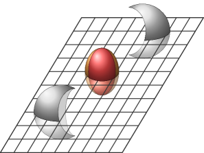
Figure 1: Sketch of a peripheral heavy ion collision. The almond shaped overlap region forms a quark-gluon plasma, not the spectator portions (shown in grey). The hydrodynamization time increases rapidly as one approaches the boundary of the overlap region, whose shape influences the value of the experimentally measured elliptic flow parameter $v_{2}$.

Pixels near the periphery of the overlap region of colliding nuclei, illustrated in Fig. 1, will have decreasing CM frame transverse energy density $\mu^{3}$ due to the rapid fall-off of the transverse energy density of the colliding nuclei near their periphery. Given the fact that the hydrodynamization time scales inversely with $\mu$ (7), this implies that pixels near the periphery of the overlap region (shown in orange) will enter the hydrodynamic regime much later than pixels in the middle of the overlap region. How this impacts an appropriate choice of the initial Cauchy surface used in hydrodynamic modeling, and the resulting uncertainties in estimates of, for example, the elliptic flow parameter $v_{2}$, is deserving of further study.

The remainder of this paper is organized as follows. In section 2 we review the characteristic formulation of general relativity in asymptotically anti-de Sitter spacetimes and the initial data for planar shock collisions, largely following Ref. Chesler:2013lia . Section 3 describes the numerical procedure and software used to compute shock collisions, highlighting several issues in greater detail than in Ref. Chesler:2013lia . Results are presented in section 4, followed by a brief final discussion in section 5. Readers primarily interested in results should feel free to turn directly to section 4. Additional computational details are presented in the appendix.

2 Planar shock collisions in asymptotically AdS spacetime

2.1 Characteristic formulation

As shown in Refs. Chesler:2010bi ; Chesler:2013lia ; Heller:2012km ; Fuini:2015hba ; Chesler:2015wra , the characteristic formulation of general relativity, originally developed by Bondi and Sachs Bondi:1960jsa ; Sachs:1962wk , provides a computationally effective method for handling the diffeomorphism invariance of general relativity when studying collisions dynamics in asymptotically AdS spacetimes.

The characteristic formulation is based on a null slicing of the geometry in which coordinates are directly tied to a congruence of null geodesics. We will use $X\equiv(x,r)$ to denote 5D coordinates, with $x=(x^{0},x^{i})\equiv(t,x^{i})$ representing ordinary Minkowski coordinates on the boundary of the AdS spacetime. Requiring that $t=\rm const.$ surfaces be null hypersurfaces implies that the one-form $k=\nabla t$ is null, $0=k_{A}\,k^{A}=g^{AB}k_{A}k_{B}$, which means that $g^{tt}=0$. Requiring the spatial coordinates $x^{i}$ to be constant along the null rays tangent to $k^{A}$ implies that $0=k^{A}\,\partial_{A}x^{i}=g^{AB}(\partial_{A}t)(\partial_{B}x^{i})$, which means that $g^{ti}=0$. These conditions on the contravariant components of the metric then imply that $g_{rr}=g_{ri}=0$. Hence, under these assumptions the most general line element may be written in the generalized infalling (or Eddington-Finkelstein) form,

$$ds^{2}=2dt\left[\beta(X)\,dr-A(X)\,dt-F_{i}(X)\,dx^{i}\right]+G_{ij}(X)\,dx^{i}dx^{j}\,.$$ (12)

It will be convenient to factor the spatial metric $G_{ij}$ into a scale factor $\Sigma$ times a unimodular matrix $\widehat{g}$,

$$G_{ij}(X)\equiv\Sigma(X)^{2}\>\widehat{g}_{ij}(X)\,,$$ (13)

with $\det(\widehat{g})\equiv 1$. One may fix one further condition, controlling the parameterization of the null geodesics tangent to $k^{A}$. Bondi and Sachs Bondi:1960jsa ; Sachs:1962wk chose to fix the scale factor $\Sigma(X)=r$, convenient for problems with spherical symmetry. We instead follow Chesler and Yaffe Chesler:2013lia and choose to set

$$\beta(X)=1\,.$$ (14)

This condition leaves a residual reparametrization invariance in the metric (12) consisting of radial shifts,

$$r\rightarrow\tilde{r}=r+\delta\lambda(x)\,,$$ (15)

with the shift $\delta\lambda$ depending in an arbitrary fashion on the boundary coordinates $x$. Under such a shift, the metric coefficient functions transform as

$$A(x,r) \rightarrow\widetilde{A}(x,\tilde{r})\equiv A(x,\tilde{r}{-}\delta\lambda)+\partial_{t}\,\delta\lambda(x)\,,$$ (16a)

$$F_{i}(x,r) \rightarrow\widetilde{F}_{i}(x,\tilde{r})\equiv F_{i}(x,\tilde{r}{-}\delta\lambda)+\partial_{i}\,\delta\lambda(x)\,,$$ (16b)

$$G_{ij}(x,r) \rightarrow\widetilde{G}_{ij}(x,\tilde{r})\equiv G_{ij}(x,\tilde{r}{-}\delta\lambda)\,.$$ (16c)

From these transformations of $A$ and $F_{i}$ it is apparent that they may be regarded as temporal and spatial components of a gauge field representing radial shifts. It is possible to write the Einstein equations in a manner which is manifestly covariant under radial shifts. To do so, it is convenient to define modified temporal and spatial derivatives,

$$d_{+}\equiv\partial_{t}+A(X)\,\partial_{r}\,,\qquad d_{i} \equiv\partial_{i}+F_{i}(X)\,\partial_{r}\,.$$ (17)

Given these definitions, the Einstein equations,

$$R^{AB}-\tfrac{1}{2}R\,g^{AB}+\Lambda\,g^{AB}=0\,,$$ (18)

acquire a nested structure with the schematic form,

$$\left(\partial_{r}^{2}+Q_{\Sigma}[\widehat{g}]\right)\Sigma =0\,.$$ (19a)

$$\left(\delta^{i}_{j}\,\partial_{r}^{2}+P_{F}[\widehat{g},\Sigma]_{i}^{j}\,\partial_{r}+Q_{F}[\widehat{g},\Sigma]_{i}^{j}\right)F_{j} =S_{F}[\widehat{g},\Sigma]_{i}\,.$$ (19b)

$$\left(\partial_{r}+Q_{d_{+}\Sigma}[\Sigma]\right)d_{+}\Sigma =S_{d_{+}\Sigma}[\widehat{g},\Sigma,F]\,.$$ (19c)

$$\left(\delta^{k}_{(i}\,\delta^{l}_{j)}\,\partial_{r}+Q_{d_{+}\widehat{g}}[\widehat{g},\Sigma]^{kl}_{ij}\right)d_{+}\widehat{g}_{kl} =S_{d_{+}\widehat{g}}[\widehat{g},\Sigma,F,d_{+}\Sigma]_{ij}\,.$$ (19d)

$$\partial_{r}^{2}A =S_{A}[\widehat{g},\Sigma,F,d_{+}\Sigma,d_{+}\widehat{g}]\,.$$ (19e)

$$\left(\delta^{j}_{i}\,\partial_{r}+Q_{d_{+}F}[\widehat{g},\Sigma]^{j}_{i}\right)d_{+}F_{j} =S_{d_{+}F}[\widehat{g},\Sigma,F,d_{+}\Sigma,d_{+}\widehat{g},A]_{i}\,.$$ (19f)

$$d_{+}\left(d_{+}\Sigma\right) =S_{d^{2}_{+}\Sigma}[\widehat{g},\Sigma,F,d_{+}\Sigma,d_{+}\widehat{g},A]\,,$$ (19g)

Each equation is a first or second order linear radial differential equation for the indicated metric component(s) or their modified time derivatives. The square brackets of each coefficient or source function indicates on which fields the term depends. Explicit form of these equations, for the case of planar shocks, are given in appendix A.

Given the rescaled spatial metric $\widehat{g}$ on any time slice, plus suitable boundary conditions, each radial differential equation may be integrated in turn, thereby determining both the other metric coefficients and the time derivative of $\widehat{g}$ on that time slice. The required boundary conditions may be inferred from the near-boundary behavior which can be obtained by solving equations (19a-19g) order by order in $r$. One finds Chesler:2013lia ,

$$A=\tfrac{1}{2}\left(r{+}\lambda\right)^{2}-\partial_{t}\lambda+a^{(4)}\,r^{-2}+\mathcal{O}(r^{-3})\,, F_{i} =-\partial_{i}\lambda+f_{i}^{(4)}\,r^{-2}+\mathcal{O}(r^{-3})\,,$$ (20a)

$$\Sigma=r{+}\lambda+\mathcal{O}(r^{-7})\,, \widehat{g}_{ij} =\delta_{ij}+\widehat{g}^{(4)}_{ij}\,r^{-4}+\mathcal{O}(r^{-5})\,,$$ (20b)

$$d_{+}\Sigma=\tfrac{1}{2}\left(r{+}\lambda\right)^{2}+a^{(4)}\,r^{-2}+\mathcal{O}\left(r^{-3}\right)\,, d_{+}\widehat{g}_{ij} =-2\,\widehat{g}^{(4)}_{ij}\,r^{-3}+\mathcal{O}(r^{-4})\,.$$ (20c)

The coefficients $a^{(4)}$, $f_{i}^{(4)}$ and $\widehat{g}_{ij}^{(4)}$ cannot be determined by a local near-boundary analysis. Note that $\widehat{g}_{ij}^{(4)}$ is necessarily traceless (because $\widehat{g}$ has unit determinant). These coefficients are mapped, via gauge/gravity duality, to the stress-energy tensor of the dual field theory. In our infalling coordinates this relation is given by Chesler:2013lia

$$\frac{2\pi^{2}}{N_{c}^{2}}\left<T_{\mu\nu}\right>\equiv\big{<}\widehat{T}_{\mu\nu}\big{>}=h_{\mu\nu}^{(4)}+\tfrac{1}{4}\,h_{00}^{(4)}\,\eta_{\mu\nu}\,,$$ (21)

with $h_{00}^{(4)}\equiv-2a^{(4)}$, $h_{0i}^{(4)}\equiv-f_{i}^{(4)}$, and $h_{ij}^{(4)}\equiv\widehat{g}_{ij}^{(4)}$. Here $N_{c}$ is the number of colors in the dual field theory, and $\eta=\mathrm{diag}(-1,+1,+1,+1)$ is the Minkowski metric tensor. Explicitly,

$$\big{<}\widehat{T}_{00}\big{>}=-\tfrac{3}{2}\,a^{(4)}\,,\quad\big{<}\widehat{T}_{0i}\big{>}=-f_{i}^{(4)}\,,\quad\big{<}\widehat{T}_{ij}\big{>}=\widehat{g}_{ij}^{(4)}-\tfrac{1}{2}\,a^{(4)}\,\delta_{ij}\,.$$ (22)

The radial shift parameter $\lambda(x)$ is completely undetermined in expansion (20) and may be chosen arbitrarily. As in previous work Chesler:2010bi ; Chesler:2013lia ; Heller:2012km ; Fuini:2015hba ; Chesler:2015wra , we use this freedom to set the radial position $r_{h}(x)$ of the apparent horizon equal to a fixed value,

$$r_{h}(x)=r_{h}\,.$$ (23)

It is sufficient to solve for the spacetime geometry in the region between the horizon and the boundary because information hidden behind the horizon cannot propagate outward and influence boundary observables. Thus, the choice (23) results in a convenient rectangular computational domain.

With our metric ansatz (12), demanding a fixed radial position of the apparent horizon leads to a condition on $d_{+}\Sigma$ Chesler:2013lia . To derive this condition, one may write the tangents to a radial infalling null congruence in the form $k_{A}(X)=\mu(X)\,\nabla_{A}\phi(X)$ for some scalar functions $\phi$ and $\mu$. Demanding that the one-form $k$ be null allows one to reexpress the time derivative of $\phi$ in terms of spatial derivatives. Requiring that the congruence satisfy the (affinely parameterized) geodesic equation $k^{A}k_{B;A}=0$ allows one to reexpress the time derivative of the multiplier function $\mu$ in terms of its spatial derivatives. Given these time derivatives, one may then compute the expansion $\theta=\nabla\cdot k$ on the time slice of interest. Demanding that the expansion vanish on a surface $\phi(X)=\rm const.$ implies that this surface is an apparent horizon. Applying this procedure to the metric ansatz (12) and specializing to the case $\phi(X)=r$ leads to the desired condition Chesler:2013lia ,

$$d_{+}\Sigma\big{|}_{r_{h}}=-\tfrac{1}{2}\,(\partial_{r}\Sigma)\,F^{2}-\tfrac{1}{3}\,\Sigma\,\nabla\cdot F\,.$$ (24)

This condition must hold at all times if the radial position of the horizon is to remain fixed at some given value $r_{h}$. Consequently, on every time slice the condition

$$\partial_{t}\,d_{+}\Sigma\big{|}_{r_{h}}=\partial_{t}\left[-\tfrac{1}{2}(\partial_{r}\Sigma)F^{2}-\tfrac{1}{3}\Sigma\,\nabla\cdot F\right]$$ (25)

is also required to hold. When combined with the Einstein equation (19g), this final condition leads to an elliptic differential equation for the value of the metric function $A$ on the (apparent) horizon. Explicit forms of the horizon equation (24) and the horizon stationarity condition (25) may be found in appendix A.

2.2 Solution strategy

To solve the nested form (19) of the Einstein equations, one requires appropriate boundary data which picks out the correct solution for each equation. The needed boundary conditions are determined by the homogeneous solutions of each equation and the asymptotic behavior of the desired solutions. This information is summarized in table 1. From this table one sees that a choice for the radial shift $\lambda$ along with values of the asymptotic coefficients $a^{(4)}$ and $f_{i}^{(4)}$ are needed as boundary conditions for the $\Sigma$, $F_{i}$, and $d_{+}\Sigma$ equations and serve to fix the coefficient of a homogeneous solution to the corresponding differential equation. The asymptotic coefficients $a^{(4)}$ and $f_{i}^{(4)}$, proportional to the boundary energy and momentum density, are dynamical degrees of freedom (in addition to the metric $\widehat{g}_{ij}$) and are determined by integrating the stress-energy continuity equation as discussed below. The radial shift $\lambda(x)$ will also be treated as a dynamical degree of freedom, as described below, and adjusted in a manner which ensures that the apparent horizon remains at a fixed radial position.

Given this boundary data, together with the value of $\widehat{g}$ on some given time slice, the radial differential equations (19a)–(19d) may each be integrated in turn, at every spatial location $x^{i}$, leading to a determination of $d_{+}\widehat{g}_{ij}$ on the time slice. Two boundary conditions are needed to integrate the second order equation (19e) for the metric function $A$. As seen in table 1, the value of the radial shift $\lambda$ supplies one condition. The second boundary condition is supplied by the value of $A$ at the apparent horizon, which is determined by solving the horizon stationarity condition (25).

Having determined both $d_{+}\widehat{g}$ and $A$, the actual time derivative for the rescaled spatial metric $\widehat{g}$ is then reconstructed as

$$\partial_{t}\,\widehat{g}_{ij}=d_{+}\widehat{g}_{ij}-A\,\partial_{r}\,\widehat{g}_{ij}\,.$$ (26)

Knowing $d_{+}\Sigma$ and $A$ (on a given time slice), the near boundary expansion (20) shows that the time derivative of the the radial shift $\lambda(x)$ may be extracted as

$$\partial_{t}\lambda=\lim_{r\to\infty}\left(d_{+}\Sigma-A\right).$$ (27)

Similarly, the asymptotic coefficient $\widehat{g}_{ij}^{(4)}$ determining the traceless stress tensor is extracted from the boundary limit of either $r^{4}\,(\widehat{g}_{ij}-\delta_{ij})$ or $-\tfrac{1}{2}r^{3}d_{+}\widehat{g}_{ij}$. This information then allows one to determine the time derivatives of $a^{(4)}$ and $f_{i}^{(4)}$ using the boundary stress-energy continuity equation, $\nabla^{\mu}\left<T_{\mu\nu}\right>=0$, which is an automatic consequence of the Einstein equations. Explicitly,

$$\partial_{t}\,a^{(4)}=\tfrac{2}{3}\,\partial_{i}\,f^{(4)}_{i}\,,\quad\partial_{t}\,f^{(4)}_{i}=\tfrac{1}{2}\,\partial_{i}a^{(4)}-\partial_{j}\,\widehat{g}_{ij}^{(4)}\,.$$ (28)

field	homogeneous solution(s)	near-boundary behavior
$\Sigma$	${}\sim\sigma^{(0)}\,r^{1}+\sigma^{(1)}\,r^{0}$	$\Sigma\sim r+\lambda$
$F_{i}$	${}\sim f_{i}^{(0)}\,r^{2}+f_{i}^{(4)}\,r^{-2}$	$F_{i}\sim-\partial_{i}\lambda+f_{i}^{(4)}r^{-2}$
$d_{+}\Sigma$	${}\sim a^{(4)}\,r^{-2}$	$d_{+}\Sigma\sim\frac{1}{2}\left(r{+}\lambda\right)^{2}+a^{(4)}\,r^{-2}$
$d_{+}\widehat{g}_{ij}$	${}\sim r^{-{3}/{2}}$	$d_{+}\widehat{g}_{ij}\sim-2\,\widehat{g}_{ij}^{(4)}\,r^{-3}$
$A$	${}\sim a^{(1)}\,r^{1}+a^{(2)}\,r^{0}$	$A\sim\frac{1}{2}\,(r{+}\lambda)^{2}-\partial_{t}\lambda$

Table 1: Near-boundary asymptotic behavior of the homogeneous solutions to the radial differential equations (19a)–(19e) for the indicated fields, together with the desired asymptotic behavior of physical solutions. The asymptotic coefficients $a^{(4)}$, $f_{i}^{(4)}$, and $\widehat{g}_{ij}^{(4)}$ determine respectively the energy density, momentum density, and traceless stress tensor of the dual field theory. The leading terms in the near-boundary behavior of all fields except $\Sigma$ are driven by the inhomogeneous source terms in the various equations and do not correspond to homogeneous solutions.

The above procedure, involving integration of a sequence of linear ordinary differential equations in the radial direction plus one spatial elliptic equation on the apparent horizon, determines the time derivatives of the dynamical data $\{\widehat{g}_{ij},\,\lambda,\,a^{(4)},\,f_{i}^{(4)}\}$ given initial values of this data on some time slice. These time derivatives are then input into a conventional time integrator, such as fourth order Runge-Kutta, to advance to the next time slice where the entire process repeats.

Overall, this characteristic formulation transforms the highly non-linear coupled Einstein equations into a set of nested linear ordinary differential equations and first order time evolution equations. We solve the radial differential equations, and the horizon stationarity equation, using spectral methods as described in some detail in section 3 and appendix C.

2.3 Planar shocks

By “planar shock” we mean an asymptotically anti-de Sitter solution of the vacuum Einstein equations whose boundary stress-energy tensor describes a “sheet” of energy density which moves at the speed of light in some longitudinal direction and is translationally invariant in the other two transverse spatial dimensions. For regular solutions, such a sheet of moving energy density will have some smooth longitudinal profile and non-zero characteristic thickness.

Let $\{x^{i}\}\equiv(\bm{x}_{\perp},z)$ denote spatial coordinates separated into transverse and longitudinal components, and consider shocks moving in the $\pm z$ direction. To specialize the general infalling metric ansatz (12) to the case of planar shock spacetimes, we impose translation invariance in transverse directions plus rotation invariance in the transverse plane, which implies that all metric components are functions of only of $r$ and $x_{\mp}\equiv t\mp z$, that $F_{i}$ only has a longitudinal component, and that the (rescaled) spatial metric has the form Chesler:2013lia ,

$$\widehat{g}=\mathrm{diag}(e^{B},e^{B},e^{-2B})\,.$$ (29)

Consequently,

$$ds^{2}=2dt\left(dr-A\,dt-F_{z}\,dz\right)+\Sigma^{2}\left(e^{B}\,d\bm{x}_{\perp}^{2}+e^{-2B}\,dz^{2}\right).$$ (30)

The boundary asymptotics (20) implies that the “anisotropy” function $B$ behaves as

$$B(x_{\mp},r)=b^{(4)}(x_{\mp})\,r^{-4}+O(r^{-5})\,.$$ (31)

For later computational convenience, let

$$u\equiv 1/{r}$$ (32)

denote an inverted radial coordinate, so that the spacetime boundary lies at $u=0$.

In general it does not seem possible to find analytic forms of planar shock solutions using the infalling Eddington-Finkelstein (EF) coordinates (30). But analytic solutions are available in Fefferman-Graham (FG) coordinates Chesler:2015wra ; Chesler:2010bi ; Janik . Using $\{\tilde{x}^{\mu},\tilde{\rho}\}\equiv\{\tilde{t},\tilde{\bm{x}}_{\perp},\tilde{z},\tilde{\rho}\}$ as our FG coordinates, with $\tilde{x}_{\pm}\equiv\tilde{t}\pm\tilde{z}$ and $\tilde{\rho}$ an inverted bulk radial coordinate, the metric

$$ds^{2}=\tilde{\rho}^{-2}\left(-d\tilde{x}_{+}\,d\tilde{x}_{-}+d\tilde{\bm{x}}^{2}_{\bot}+d\tilde{\rho}^{2}\right)+\tilde{\rho}^{2}\,h(\tilde{x}_{\pm})\,d\tilde{x}_{\mp}^{2}\,,$$ (33)

is a planar shock solution describing a shock moving in the $\pm z$ direction with arbitrary longitudinal energy density profile $h(z)$. In the calculations described below, we use simple Gaussian profiles with width $w$ and longitudinally integrated energy density $\mu^{3}$,

$$h(z)\equiv\mu^{3}(2\pi w^{2})^{-1/2}\,e^{-\frac{1}{2}z^{2}/w^{2}}\,.$$ (34)

The associated boundary stress-energy tensor is just

$$\widehat{T}^{00}(\tilde{t},\tilde{z})=\widehat{T}^{zz}(\tilde{t},\tilde{z})=\pm\widehat{T}^{0z}(\tilde{t},\tilde{z})=h(\tilde{t}{-}\tilde{z})\,,$$ (35)

with all other components vanishing.

Focusing, for ease of presentation, on shocks moving in the $+z$ direction, the translational symmetries imply that the EF and FG coordinates will be related by a transformation of the form Chesler:2013lia ,

$$\tilde{t}=t+u+\alpha(t{-}z,u)\,,\quad\tilde{z}=z-\gamma(t{-}z,u)\,,\quad\tilde{\rho}=u+\beta(t{-}z,u)\,,$$ (36)

and $\tilde{\bm{x}}_{\bot}=\bm{x}_{\bot}$.

As discussed above, the required initial data for the characteristic evolution scheme consists of the anisotropy function $B$ plus the boundary data $\{a^{(4)},\,f_{z}^{(4)}\}$ and the radial shift $\lambda$. Inserting a transformation of the form (36) into the FG metric (33), a short exercise Chesler:2013lia shows that

$$B=-\tfrac{1}{3}\ln\big{[}-(\partial_{z}\alpha)^{2}+(\partial_{z}\beta)^{2}+(1-\partial_{z}\gamma)^{2}+(u+\beta)^{4}(1-\partial_{z}\alpha-\partial_{z}\gamma)^{2}\,h\big{]}\,,$$ (37)

while the boundary data is given by

$$a^{(4)}=-\tfrac{2}{3}\,h\,,\qquad f^{(4)}_{z}=h\,,\qquad\lambda=-\tfrac{1}{2}\,\partial_{u}^{2}\beta\big{|}_{u=0}\,.$$ (38)

To solve for the transformation functions $\{\alpha,\beta,\gamma\}$, one approach, used in Refs. Chesler:2010bi ; Chesler:2013lia , is to insert the transformation (36) into the FG metric (33) and demand that the result have the EF form (30). To simplify the resulting equations, it is helpful to redefine the transformation functions $\alpha$ and $\beta$ via

$$\alpha=-\gamma+\beta+\delta\,,\qquad\beta=-\frac{u^{2}\zeta}{1+u\zeta}\,.$$ (39)

One finds Chesler:2013lia that the functions $\zeta$ and $\delta$ satisfy a pair of coupled differential equations,

$$\frac{1}{u^{2}}\frac{\partial}{\partial u}\left(u^{2}\,\frac{\partial\zeta}{\partial u}\right)+\frac{2uH}{(1+u\zeta)^{5}}=0\,,\qquad\frac{\partial\delta}{\partial u}-\frac{u^{2}}{(1+u\zeta)^{2}}\,\frac{\partial\zeta}{\partial u}=0\,,$$ (40a)

while $$\gamma$$ satisfies a decoupled equation,

$$\frac{\partial\gamma}{\partial u}-\frac{u^{2}}{(1+u\zeta)^{2}}\,\frac{\partial\zeta}{\partial u}+\frac{u^{4}}{2(1+u\zeta)^{2}}\left(\frac{\partial\zeta}{\partial u}\right)^{2}+\frac{u^{4}H}{2(1+u\zeta)^{6}}=0\,,$$ (40b)

with $$H\equiv h+\left(t-z+u+\delta-u^{2}\zeta/(1+u\zeta)\right)$$. The desired solutions have the near-boundary behavior

$$\zeta\sim\lambda+O(u^{3})\,,\quad\delta\sim O(u^{5})\,,\quad\gamma\sim O(u^{5})\,.$$ (40c)

Integrating equations (40) with boundary conditions ensuring the behavior (40c), and inserting the resulting transformation functions into Eqs. (37) and (38), yields the anisotropy function $B$ and associated boundary data describing of a single shock.

To construct initial data for colliding shocks, we superpose counter-propagating single shock data at an initial time $t_{0}$ when the two shocks are sufficiently widely separated that their overlap is negligible,

$$B(u,z,t_{0}) =B_{+}(u,t_{0}{-}z)+B_{-}(u,t_{0}{+}z)\,,$$ (41a)

$$a^{(4)}(z,t_{0}) =a_{+}^{(4)}(t_{0}{-}z)+a_{-}^{(4)}(t_{0}{+}z)\,,$$ (41b)

$$f_{z}^{(4)}(z,t_{0}) =f_{z+}^{(4)}(t_{0}{-}z)-f_{z-}^{(4)}(t_{0}{+}z)\,.$$ (41c)

However, unlike for the other functions, the overlap of the radial shifts $\lambda_{\pm}$ of the left and right moving shocks in the region close to $z\,{=}\,0$ is significant. Since we choose the shocks on the first time slice to be well separated, we may regard the geometry in between as deviating negligibly from pure AdS. This justifies modifying the initial shift function $\lambda$ in the neighborhood of $z=0$, without changing the physical data $\{B(u,z,t_{0}),\,a^{(4)}(z,t_{0}),\,f^{(4)}(z,t_{0})\}$. As in Ref. Chesler:2013lia , we adjust the initial radial shift by setting

$$\lambda(z,t_{0})=\theta_{+}(-z)\,\lambda_{+}(t_{0}{-}z)+\theta_{-}(z)\,\lambda_{-}(t_{0}{+}z)\,,$$ (42)

with $\theta_{\pm}(z)\equiv\frac{1}{2}\left[1-\mathrm{erf}(-z/(\sqrt{2}w_{\pm}))\right]$ a smoothed step function.

In practice, we slightly modify the above superposition procedure. Following Refs. Chesler:2013lia ; Chesler:2010bi , we replace Eq. (41b) with

$$a^{(4)}(z,t_{0})=a_{+}^{(4)}(t_{0}{-}z)+a_{-}^{(4)}(t_{0}{+}z)-\tfrac{2}{3}\,\epsilon_{0}\,.$$ (43)

From the form (22) of the stress-energy tensor, one sees that $\epsilon_{0}$ is a constant additive shift in $\widehat{T}^{00}$. In other words, $\epsilon_{0}$ is an (artificial) uniform background energy density. Adding a small background energy density helps alleviate numerical problems, as discussed below, and physically means that the colliding shocks will be propagating through a background thermal medium. If the background energy density $\epsilon_{0}$ is sufficiently small compared to the energy densities in the colliding shocks, then the background will effectively be very cold (compared to the energy scale $\mu$ of the shocks) and there will be little dissipation to the medium. This modification is done purely for numerical convenience and we will be interested in results extrapolated to vanishing background energy density.

3 Computational methods and software construction

The aim of this section is to describe the construction of a planar shockwave collision code in sufficient detail so that an interested reader could create their own version with relatively modest effort. Those primarily interested in results should skip to the next section.

3.1 Transformation to infalling coordinates

As explained in Ref. Chesler:2013lia and the previous section, the transformation from Fefferman-Graham to infalling coordinates may be computed by first solving for the congruence of infalling geodesics in FG coordinates. Or, in the special case of planar shock geometries, one can directly solve the simplified transformation equations (40). We implemented both approaches, and found them to have comparable numerical efficiency. Here, we focus on the direct approach of solving Eqs. (40) for the case of a right moving shock. Henceforth, for convenience, we also set $\mu\,{=}\,1$. Appropriate factors of $\mu$ can always be reinserted via dimensional analysis.

We solve the coordinate transformation equations (40) in the rectangular region $u\in[0,u_{\rm end}]$, $z\in[-L_{z}/2,L_{z}/2]$ using Newton-Raphson iteration (i.e., linearizing each equation in the deviation of the solution from the current approximation), and solving the resulting linear equations using spectral methods with domain decomposition.

Periodic boundary conditions are imposed in the longitudinal direction and functions of $z$ are approximated as truncated Fourier series. This is exactly equivalent to characterizing any function $f(z)$ by a list of its values, $\{f_{l}\equiv f(z_{l})\}$, on an evenly spaced Fourier grid composed of $N_{z}$ points,

$$z_{l}\equiv L_{z}(-\tfrac{1}{2}+l/N_{z})\,,$$ (44)

for $k=0,{\cdots},N_{z}{-}1$. Derivatives with respect to $z$ turn into the application of a Fourier grid differentiation matrix $D_{z}=\|(D_{z})_{kl}\|$ applied to the vector of function values,

$$f^{\prime}(z_{k})=\sum_{l}(D_{z})_{kl}\,f_{l}\,.$$ (45)

Explicit expressions for the Fourier grid differentiation matrix components $(D_{z})_{kl}$ are given in appendix C. A rather fine longitudinal grid is required to accurately represent thin shocks within a large longitudinal box. We used Fourier grids with $N_{z}\,{=}\,960$ for $L_{z}\,{=}\,12$ and shock widths down to $0.075$.

To represent the dependence of functions on the radial coordinate $u$ we first decompose the domain $[0,u_{\rm end}]$ into $M$ equally sized subdomains, and then use a Chebyshev-Gauss-Lobatto grid with $N_{u}$ points within each subdomain. This amounts to using a radial grid composed of the points

$$u_{jk}\equiv\frac{u_{\rm end}}{2M}\left(2j-1-\cos\frac{\pi k}{N_{u}{-}1}\right),$$ (46)

for $j=1,{\cdots},M$ and $k=0,{\cdots},N_{u}{-}1$. The radial dependence of some function $g(u)$ is represented by the list of $M\times N_{u}$ function values on this grid, $\{g_{jk}\equiv g(u_{jk})\}$, and derivatives with respect to $u$ turn into the application of a (block diagonal) Chebyshev differentiation matrix $D_{u}$ applied to this list of function values,

$$g^{\prime}(u_{jk})=\sum_{l}(D_{u})_{kl}\,g_{jl}\,.$$ (47)

Explicit expressions for the components of the Chebyshev differentiation matrix $D_{u}$ are given in Eq. (102). As discussed in Ref. Chesler:2013lia , using domain decomposition (i.e., $M>1$) helps to avoid excessive precision loss in the numerical evaluation of equations near the $u=0$ boundary, and allows the use of a larger time step without running afoul of CFL instabilities. To integrate radial equations down to $u_{\rm end}\,{=}\,2$, we used radial grids with up to $M\,{=}\,22$ domains and $N_{u}\,{=}\,12$ points within each subdomain.

The product of these 1D grids defines our 2D spectral grid. Any function $f(u,z)$ becomes a set of $N_{\rm tot}\equiv M\times N_{u}\times N_{z}$ values on these grid points,

$$\{f_{jkl}\equiv f(u_{jk},z_{l})\}\,.$$ (48)

Fortunately, the differential equations (40) are completely local in $z$. So these equations, evaluated on the 2D grid with derivatives replaced by the corresponding differentiation matrices, do not become a single set of $2N_{\rm tot}$ (for Eq. 40a) or $N_{\rm tot}$ (for Eq. 40b) coupled algebraic relations. Rather they yield $N_{z}$ decoupled systems, each involving $2MN_{u}$ (for Eq. 40a) or $MN_{u}$ (for Eq. 40b) variables.

For each set of equations, linearization around some initial, or current, guess for a solution leads to a set of linear equations of the generic form $\mathcal{M}\,f=-S$, where $f$ is the unknown vector of function deviations from the current guess, $S$ is the vector of residuals, and $\mathcal{M}$ is the spectral approximation to the linear operator which results from the linearization of the differential equation(s) at some given value of $z$.

At this point, these linear equations are singular. First, $u\,{=}\,0$ is a regular singular point of the differential equations (40a) and (40b); one cannot simply evaluate, numerically, these equations at $u\,{=}\,0$. Moreover, solutions to these differential equations are, of course, non-unique. One must complement the differential equations with suitable boundary conditions to specify a unique solution. With spectral methods, fixing one of these problems fixes the other. Prior to linearization, one simply replaces the (ill-defined) evaluation of the equations at $u\,{=}\,0$ by constraints encoding required boundary conditions.

Examining equations (40a) and (40b), one sees that the most general near-boundary behavior is

$$\zeta\sim\zeta_{-1}\,u^{-1}+\lambda+O(u^{3})\,,\quad\gamma\sim\gamma_{0}+O(u^{5})\,,\quad\delta\sim\delta_{0}+O(u^{5})\,,$$ (49)

for arbitrary values of the coefficients $\zeta_{-1}$, $\lambda$, $\gamma_{0}$ and $\delta_{0}$. We want to set the leading coefficients $\zeta_{-1}$, $\gamma_{0}$ and $\delta_{0}$ to zero. To implement this Dirichlet condition for $\gamma$ and $\delta$ in a manner which avoids unnecessary precision loss when computing derivatives of these functions at the boundary, it is convenient first to redefine

$$\gamma(z,u)\equiv u^{3}\,\tilde{\gamma}(z,u)\,,\quad\delta(z,u)\equiv u^{3}\,\tilde{\delta}(z,u)\,,$$ (50)

and then reexpress equations (40) in terms of $\tilde{\gamma}$ and $\tilde{\delta}$. Unwanted solutions with non-zero boundary values for $\gamma$ or $\delta$ are then simply not representable when using our spectral representation for $\tilde{\gamma}$ or $\tilde{\delta}$. Similarly, using our spectral representation for $\zeta$ automatically eliminates unwanted solutions where $\zeta$ has singular $1/u$ behavior.

The continuum differential equations imply that $\tilde{\gamma}$ and $\tilde{\delta}$ both vanish, and have vanishing first derivatives, at the boundary. To deal with the $u\,{=}\,0$ regular singular point in the discretized equations for $\tilde{\gamma}$ and $\tilde{\delta}$ it is sufficient to replace the equations at $u\,{=}\,0$ with constraints setting $\tilde{\gamma}$ and $\tilde{\delta}$ to zero. If we wished to fix the radial shift $\lambda$ by simply specifying its value, we could similarly redefine $\zeta=\lambda+u\,\tilde{\zeta}$ and require $\tilde{\zeta}$ to vanish at the boundary. However, we found it more convenient to fix $\lambda$ indirectly by demanding that $\zeta$ vanish at our chosen value of $u_{\rm end}$. Referring to Eqs. (36) and (39), one sees that this condition will make the $u=u_{\rm end}$ surface coincide with a surface of constant FG radial coordinate, $\tilde{\rho}=u_{\rm end}$. In other words, with this condition the FG computational domain $\tilde{\rho}\in[0,\tilde{\rho}_{\rm end}]$ is the same as the EF domain $u\in[0,u_{\rm end}]$.

The net effect of the above procedure, in the discretized equations for $\zeta$, $\tilde{\delta}$ and $\tilde{\gamma}$ at longitudinal position $z_{l}$, is to replace the the (degenerate) equations at $u\,{=}\,0$ by the respective constraints

$$\zeta_{M,N_{u}-1,l}=0\,,\quad\tilde{\delta}_{1,0,l}=0\,,\quad\tilde{\gamma}_{1,0,l}=0\,.$$ (51)

In addition to applying boundary conditions at $u\,{=}\,0$, when using domain decomposition one must also impose continuity conditions at subdomain boundaries. Our set (46) of radial grid points redundantly duplicates the interior endpoints of each subdomain, $u_{j,N_{u}-1}=u_{j+1,0}$ for $j=1,{\cdots},M{-}1$, and hence two different rows of the linear equation $\mathcal{M}f=-S$ represent the differential equation evaluated at the same physical point. One could deal with this by eliminating the duplication of subdomain endpoints and suitably redefining the differentiation matrix $D_{u}$. But it is even easier to fix the problem by simply replacing one of the rows representing an interior subdomain endpoint with a constraint equation enforcing the equality of duplicated function values at this point, $f_{j,N_{u}-1,l}-f_{j+1,0,l}=0$.

After these row replacements, the modified linear system is reasonably well conditioned and, with a sufficiently good initial guess, Newton iteration rapidly converges quadratically. To generate an initial guess, it is natural to work sequentially in $z$. If the shock is propagating in the $+z$ direction with the profile function $h(z)$ having its maximum at $z\,{=}\,0$, then at the furthest point behind the shock, $z_{0}=-L_{z}/2$, the geometry deviates negligibly from pure AdS and $\zeta=\tilde{\gamma}=\tilde{\delta}=0$ is a fine initial guess. Thereafter, we use the converged solution at each $z_{i}$ as an initial guess for the solution at $z_{i+1}$. This provides a good initial guess provided the longitudinal grid spacing is sufficiently fine.

The above procedure for solving the transformation equations (40) using spectral methods works well as long as the radial depth $u_{\rm end}$ to which one integrates is not too large. The key advantage of this approach is that the precision of the obtained solutions do not degrade near the boundary, even through $u\,{=}\,0$ is a singular point of the differential equations. That is to say, spectral methods are excellent for finding well-behaved solutions of equations having regular singular points. However, as $u_{\rm end}$ increases the linear operators one inverts in this Newton iteration scheme become increasingly ill-conditioned. Unfortunately, the depth to which one must integrate in order to locate the apparent horizon (discussed next) after superposing shocks grows with increasing separation of the initial shocks. We used two strategies to cope with this difficulty.

First, following Refs. Chesler:2013lia ; Chesler:2010bi , we added a small artificial background energy density $\epsilon_{0}$ when superposing shocks as described above. Increasing the background energy density decreases the depth at which an apparent horizon forms. Second, after using the above approach to find the transformation functions for $u<u_{\rm end}$, we integrate further into the bulk by switching to an adaptive 4th order Runge-Kutta integrator, with the spectral solution at $u_{\rm end}$ providing initial data. (A description of this standard integrator is given in appendix E.) For simplicity, we choose to integrate to a fixed value $u=u_{\rm max}$, instead of a fixed value of $\tilde{\rho}$.

For our chosen range of shock parameters, with widths down to $w\,{=}\,0.075$, using a spectral grid down to $u_{\rm end}\,{=}\,2$ worked well. With a longitudinal box size $L_{z}\,{=}\,12$ and background energy densities in the range of 1–5% of the peak energy density, it turned out that only a modest further integration with the adaptive integrator down to $u_{\rm max}=2.11$ was sufficient to reach the apparent horizon throughout the longitudinal box. Having transformed a right-moving single shock solution to infalling coordinates, and extracted the resulting initial data $\{B_{+},a_{+}^{(4)},f_{z+}^{(4)},\lambda_{+}\}$ for evolution using Eqs. (37)–(38), a simple reflection generates corresponding data for a left-moving shock,

$$B_{-}(u,z) =B_{+}(u,-z)\,, a_{-}^{(4)}(z) =a_{+}^{(4)}(-z)\,,$$ (52a)

$$\lambda_{-}(z) =\lambda_{+}(-z)\,, f_{z-}^{(4)}(z) =-f_{z+}^{(4)}(-z)\,.$$ (52b)

We construct initial data for counter-propagating shocks by combining single shock solutions as described earlier in Eqs. (41)–(43). We chose the initial time $t_{0}$ for this superposition so that the initial separation between the shocks, $\Delta z_{0}=-2t_{0}$, is large compared to the shock widths. We used $\Delta z_{0}=4$ for symmetric collisions of broad shocks, $\Delta z_{0}=2$ for symmetric collisions of thin shocks, and $\Delta z_{0}=3$ for asymmetric collisions of shocks.

For thin shockwave collisions with small background energy density, avoiding numerical instabilities associated with short wavelength perturbations is challenging. As discussed in Ref. Chesler:2013lia , it is helpful to damp discretization induced perturbations using appropriate filtering. We constructed and applied smoothing filters to the initial data in both longitudinal and radial directions. Details of these filters are presented in appendix D.2.

3.2 Horizon finding

After transforming chosen single shock solutions to infalling coordinates, as just discussed, and combining two counter-propagating shocks as shown in Eqs. (41)–(43)), the final step in the construction of initial data is locating the apparent horizon which serves as an IR cutoff in the bulk.

In our planar shock geometries, the apparent horizon condition (24) becomes

$$0=d_{+}\Sigma+\frac{e^{2B}}{6\Sigma^{2}}\left(3F^{2}\,\partial_{r}\Sigma+2\Sigma\,\partial_{z}F+4F\,\Sigma\,\partial_{z}B+2F\,\partial_{z}\Sigma\right)\Big{|}_{r=r_{h}}.$$ (53)

A radial shift, $r=\bar{r}+\delta\lambda$, corresponds in our inverted radial coordinates to

$$u=\frac{\bar{u}}{1+\bar{u}\,\delta\lambda}\,.$$ (54)

If $\bar{u}\in[0,u_{\rm max}]$ represents the radial coordinate used in the transformation to infalling coordinates, then we wish to determine the value of a further shift $\delta\lambda(z)$ such that condition (53) holds at some value of $u_{h}\equiv 1/r_{h}$ which may, for convenience, be chosen to equal the same value $u_{\rm max}$ from the coordinate transformation. With this choice, $\delta\lambda$ must be negative for the sought-after apparent horizon to lie within the coordinate transformation domain.

Equation (53) is a nonlinear but ordinary differential equation for the shift function $\delta\lambda(z)$. To solve it, we use spectral methods (with the same Fourier grid in $z$) combined with a root finding routine. Linearizing equation (53) in $\delta\lambda$ allows us to apply Newton iteration. Each iteration step starts with a trial value of the radial shift, $\delta\lambda^{(m)}$ in iteration $m$, and computes the residual (i.e., the right-hand side of Eq. (53)) and its variation with respect to $\delta\lambda$, and solves the linearized equation to find an improved value $\delta\lambda^{(m+1)}$ of the shift.

To evaluate the residual and its variation, we first integrate Eqs. (19a)–(19c), using the current value of $B(z,u)$ and $\lambda(z)$, to find the auxiliary functions $\Sigma$, $F$ and $d_{+}\Sigma$. After each step we convert the spectral representation of $B(z,u)$ to a new radial grid with grid points shifted according to Eq. (54). To do so, we perform off-grid interpolation using a sum of Chebyshev cardinal functions Boyd:Spectral with coefficients given by the on-grid values of $B(z,u)$.

For our settings of longitudinal box size and shock parameters, we found it advantageous to choose the initial guess $\delta\lambda^{(0)}$ to be $0.1$. It was also helpful to start with a relatively large background energy density $\epsilon_{0}$ of about $10\%$ of the peak shock energy density, and then gradually decrease $\epsilon_{0}$ during each iteration step until it reached the desired final value before Newton iteration convergence.

During time evolution, described next, solving the horizon stationarity condition (25) on each time step yields the time derivative of the radial shift thereby providing the information needed to integrate $\lambda$ forward in time. (The explicit form of Eq. (25) for our planar shock geometries is given in Eq. (73).) To prevent discretization errors from driving long term drift away from the desired horizon condition (53), we also directly recomputed the apparent horizon position every 10–100 time steps using the above iterative procedure.

3.3 Time evolution

As described above in section (2.2), the data on any time slice needed to integrate forward in time consists of $\{B(z,u),\,a^{(4)}(z),\,f^{(4)}(z),\,\lambda(z)\}$. To compute the time derivative of this data, we successively solve Eqs. (19a)–(19e) as discussed earlier. Explicit forms of these equations are given in Eqs. (71a)–(71e) of appendix A. We use the same multi-domain spectral methods described above in section 3.1. These methods presume that functions being represented by their values on the spectral grid are well behaved throughout the computational domain. Our functions $\Sigma$ and $A$ have divergent near-boundary behavior, as shown in Table 1, so for computational purposes we use redefined functions in which the leading near-boundary behavior is subtracted. For most functions, we also choose redefinitions such that the new functions either have known non-zero boundary values or vanish linearly at the boundary. Specifically, we use the following redefinitions,

$$B(u,z,t) =\Big{(}\frac{u}{1+u\lambda}\Big{)}^{3}\>b(u,z,t)\,,$$ (55a)

$$\Sigma(u,z,t) =\Big{(}\frac{u}{1+u\lambda}\Big{)}^{-1}+\Big{(}\frac{u}{1+u\lambda}\Big{)}^{4}\>\sigma(u,z,t)\,,$$ (55b)

$$F_{z}(u,z,t) =-\partial_{z}\lambda+\Big{(}\frac{u}{1+u\lambda}\Big{)}^{2}\>f(u,z,t)\,,$$ (55c)

$$d_{+}\Sigma(u,z,t) =\tfrac{1}{2}\Big{(}\frac{u}{1+u\lambda}\Big{)}^{-2}+\Big{(}\frac{u}{1+u\lambda}\Big{)}^{2}\>d_{+}\sigma(u,z,t)\,,$$ (55d)

$$d_{+}B(u,z,t) =\Big{(}\frac{u}{1+u\lambda}\Big{)}^{2}\>d_{+}b(u,z,t)\,,$$ (55e)

$$A(u,z,t) =\tfrac{1}{2}\Big{(}\frac{u}{1+u\lambda}\Big{)}^{-2}+a(u,z,t),$$ (55f)

We use factors of $u/(1+u\lambda)=(r+\lambda)^{-1}$ in these redefinitions, instead of pure powers of $u$, so that the new functions transform simply under radial shifts. This is natural as it preserves manifest radial shift covariance in the equations for the new functions, but is not essential. In relations (55d) and (55e), and henceforth, $d_{+}\sigma$ and $d_{+}b$ are simply names for redefined functions encoding $d_{+}\Sigma$ and $d_{+}B$, respectively, and are not themselves modified $d_{+}$ time derivatives applied to $\sigma$ or $b$.

Referring to Table 1 and Eq. (20), one sees that the new functions $b$ and $d_{+}b$ vanish linearly as $u\to 0$, while $f$ and $d_{+}\sigma$ have non-zero boundary values of $f_{z}^{(4)}$ and $a^{(4)}$, respectively. The new function $a$ has a boundary value of $-\partial_{t}\lambda$ which is an output, not an input, of the radial integration determining $a$.

Arranging to have constant or linear near-boundary behavior of redefined functions minimizes the precision loss which can occur when evaluating derivatives very near the boundary. In particular, extracting the third power of $u/(1+u\lambda)$ in the definition (55a) of $b$ is essential for the numerical stability.

After inserting the redefinitions (55) into the relevant radial equations (71a)–(71e), it is crucial to simplify the resulting equations, prior to numerical implementation, in such a way that cancellations of terms with the most divergent near-boundary behavior are performed exactly, analytically. When each radial differential equation is written in canonical form (with a unit coefficient of the highest order $u$-derivative), no term in the inhomogeneous source term of the equation should be more singular than $1/u$ for first order and $1/u^{2}$ for second order equations, otherwise unnecessary precision loss will occur during the numerical evaluation of the equation.

In solving the successive radial equations Eqs. (19a)–(19e) [or (71a)–(71e)], we implement the following boundary conditions at $u\,{=}\,0$ using the row replacement technique described in section 3.1,

$$\sigma(0,z)=0\,,\quad f(0,z)=f^{(4)}(z)\,,\quad d_{+}\sigma(0,z)=a^{(4)}(z)\,,\quad d_{+}b(0,z)=0\,.$$ (56)

Equation (19a) [or (71a)] for $\Sigma$ is a second order differential equation, but after conversion to an equation for $\sigma$ both homogeneous solutions are divergent at the boundary and lie outside our spectral representation function space. Using row replacement to encode $\sigma(0,z)\,{=}\,0$ (which is an automatic consequence of the differential equation for $\sigma$) is the easiest way to handle the singular boundary point on the spectral grid. For the $F$ equation (19b) [or (71b)], after conversion to an equation for $f$ only one boundary condition fixing the coefficient $f_{z}^{(4)}$ of the normalizable homogeneous solution is needed as the spectral representation for $f$ automatically precludes any non-normalizable homogeneous solution. Likewise for the $d_{+}\Sigma$ equation (19c) [or (71c)], a single boundary condition fixing the coefficient $a^{(4)}$ of the normalizable homogeneous solution is needed. For the $d_{+}B$ equation (19d) [or (71d)], after conversion to an equation for $d_{+}b$ the one homogeneous solution is again outside the spectral representation function space, and encoding $d_{+}b(0,z)\,{=}\,0$ via row replacement is again the easiest way to handle the singular boundary point.

Finally, for the $A$ equation (19e) [or (71e)], after conversion to an equation for the new function $a$ the non-normalizable homogeneous solution is automatically excluded by the spectral representation for $a$. One boundary condition is needed to fix the coefficient of the normalizable homogeneous solution. Referring to table 1, specifying the boundary value of $a$ is the same as fixing the time derivative of the radial shift, $a(0,z)=-\partial_{t}\lambda(z)$. But we do not wish to input some arbitrary choice for this time derivative. Instead, prior to solving the $A$ equation (19e) we first solve the horizon stationarity condition (25) which determines the value of $A$ on the horizon. This is an inhomogeneous differential equation involving $A$ and its first and second order longitudinal derivatives, evaluated on the horizon. The explicit form is given in (73) of appendix A. Then, to solve the radial equation (19e) [or (71e)], converted to an equation for $a$, we replace the $u\,{=}\,0$ row in the spectral discretization of this equation with a row fixing the value of $a$ at the horizon, i.e., equating $a(u_{\rm max},z)$ to the value determined by the horizon stationarity condition.

To recap, every time step begins with the sequential solution of equations (71a)–(71e), plus the horizon stationarity condition, using the same spectral methods and Chebyshev grid employed in the preparation of initial data. This yields $\Sigma$, $F$, $d_{+}\Sigma$, $d_{+}B$ and $A$, from which the ordinary time derivatives of $B$, $a^{(4)}$, $f_{z}^{(4)}$ and $\lambda$ are extracted using relations (26)–(28). This is the information needed to integrate forward in time.

To perform time integration we use a discrete approximation with non-zero time step $\delta t$. We specifically choose the well known fourth order Runge-Kutta method (RK4), which uses four “substeps” each involving the evaluation of time derivatives, performed as described above for each point on our longitudinal grid. (The relevant RK4 formulas are shown in appendix E.)

A time step $\delta t=0.002$ was used in all integrations, which was sufficient to deliver stable evolution for all shock widths considered. For broader shocks ($w>0.3$) a lower order time integrator would have sufficed, but for shocks with width $w<0.1$ we found using at least RK4 to be essential, with our time step, to achieve accurate results. After each time step of the evolution we filter the final results for the propagating data $\{B,a^{(4)},f^{(4)},\lambda\}$ in the longitudinal direction using a low-pass filter, as detailed in D, which damps the upper third of the spectral bandwidth. The filtering is applied to the final RK4 outputs, not during the RK4 substeps. This damps short wavelength discretization-dependent fluctuations; such filtering should be viewed as a part of the spectral discretization prescription. We do not apply filtering to any interim results while solving the radial equations (19a)–(19e).

4 Results

4.1 Calculated collisions

Using the above described techniques and associated software, planar shock collisions were computed for various combinations of incoming shock widths. All initial shocks had Gaussian profiles (34) and identical transverse energy density $\mu^{3}$. In units in which $\mu\equiv 1$, shock widths ranged between 0.075 and 0.35. For technical reasons involving the damping of numerical artifacts, as discussed above, an artificial background energy density was added whose size ranged from $5.5\%$ down to $1.2\%$ of the peak energy density of the narrower shock. Periodic boundary conditions were applied in the longitudinal direction, with this dimension then discretized with a uniformly spaced (Fourier) grid having of up to $N_{z}=720$ points. The longitudinal period $L_{z}$ was set to 10, 11, or 12 for collisions of narrow, asymmetric, or broad shocks, respectively. In the radial direction, domain decomposition with $M=22$ subdomains of uniform size in the inverted radial coordinate $u=1/r$ was used, with a Chebyshev-Gauss-Lobatto grid of $N_{u}=13$ points within each subdomain. Time evolution used RK4 time-stepping with a step size $\delta t=0.002$ and total time duration ranging from $t=5/\mu$ to $t=6/\mu$. Table 2 lists the parameters of specific calculations.

run	$w_{+}$	$w_{-}$	$N_{z}$	$\epsilon_{0}$
1	0.35	0.35	720	$\{0.055,\,0.066\}$
2	0.25	0.25	480	$\{0.039,\,0.045\}$
3	0.1	0.25	660	$\{0.015,\,0.017\}$
4	0.1	0.1	600	$\{0.015,\,0.017\}$
5	0.075	0.35	660	$\{0.012,\,0.015\}$
6	0.075	0.25	660	$\{0.012,\,0.015\}$
7	0.075	0.075	600	$\{0.012,\,0.015\}$

Table 2: Physical and computational parameters of specific computed collisions. Shown are the incoming shock widths $w_{\pm}$, number of longitudinal grid points $N_{z}$, and background energy densities $\epsilon_{0}$. Shock widths $w_{\pm}$ are measured in units of $\mu^{-1}$. The background energy density $\epsilon_{0}$ is in units of the peak energy density of the narrower shock, or $\mu^{3}w_{+}^{-1}/\sqrt{2\pi}$. Computed results at the two listed values of $\epsilon_{0}$ were used to extrapolate to vanishing background energy density.

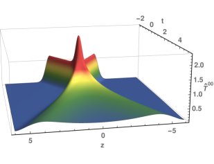
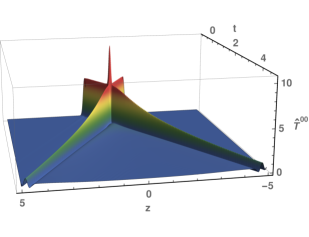
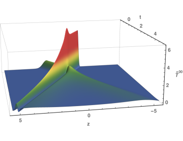
Figure 2: The energy density $\widehat{T}^{00}(t,z)$ plotted as a function of time $t$ and longitudinal position $z$ for symmetric collisions with shock width $w_{\pm}=0.35/\mu$ (upper left) and $w_{\pm}=0.075/\mu$ (upper right), and the corresponding asymmetric collision (bottom) involving shocks of widths $(w_{+},w_{-})=(0.075/\mu,0.35/\mu)$. All shocks have equal transverse energy density $\mu^{3}$.

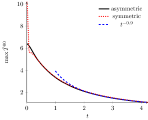
Figure 3: Comparison of time dependent amplitudes of the energy density maxima (associated with the thinnest shock) in a symmetric collision of two narrow shocks of width $w=0.075$ (solid blue line) and an asymmetric collision of shocks having widths $w=0.075$ and $w=0.25$ (dashed red line), with all incoming shocks having the same transverse energy density. Also shown is a $t^{-0.9}$ asymptotic form (long dashed blue line). Except for short time transients ($t\lesssim 0.3$), the maxima in the symmetric and in the asymmetric case behave identically. For $t\gtrsim 1.5$ the amplitude decrease is well described as $t^{-0.9}$, as previously found in Ref. Chesler:2013lia .

Figure 2 shows the energy density $\widehat{T}^{00}(t,z)$, in units of $\mu^{4}$, for three representative collisions. The top row shows symmetric collisions of shocks with widths $w_{\pm}=0.35$ (upper left) and $w_{\pm}=0.075$ (upper right), while the lower row displays results from the corresponding asymmetric collision with $(w_{+},w_{-})=(0.075,0.35)$.

Local maxima in the energy density are present on the forward lightcone, as clearly seen in Fig. 2. These local maxima lie outside the hydrodynamic region (discussed below). In asymmetric collisions, the width of a given postcollision local maxima largely reflects the width of the corresponding incoming projectile. As shown in Fig. 3, the amplitude of these local maxima decay with the same power-law time dependence seen in symmetric collisions.

4.2 Hydrodynamic flow

At every spacetime event inside the forward lightcone of a collision, the timelike eigenvector and corresponding eigenvalue of the holographically computed stress-energy tensor determine the fluid 4-velocity $u^{\mu}$ and proper energy density $\epsilon$,

$${\widehat{T}^{\mu}}{}_{\nu}\,u^{\nu}=-\epsilon\,u^{\mu}\,,$$ (57)

with normalization $u^{\mu}u_{\mu}=-1$ and $u^{0}>0$. Given the flow velocity and energy density, we use the first order hydrodynamic constitutive relation to construct the hydrodynamic approximation to the stress-energy tensor,

$$\widehat{T}^{\mu\nu}_{\rm hydro}=p\,g^{\mu\nu}+(\epsilon{+}p)\,u^{\mu}u^{\nu}+\Pi^{\mu\nu}\,,$$ (58)

where the viscous stress (to first order in gradients) is given by

$$\Pi_{\mu\nu}=-\eta\,\left[\partial_{(\mu}u_{\nu)}+u_{(\mu}u^{\rho}\partial_{\rho}u_{\nu)}-\tfrac{1}{3}\,\partial_{\alpha}u^{\alpha}(\eta_{\mu\nu}+u_{\mu}u_{\nu})\right]+\mathcal{O}(\partial^{2})\,.$$ (59)

For the conformal fluid of $\mathcal{N}\,{=}\,4$ Yang-Mills theory, the pressure $p=\epsilon/3$ and the shear viscosity $\eta=(\epsilon/3)^{3/4}/\sqrt{2}$.

Following Ref. Chesler:2015fpa , we define the spacetime region $\mathcal{R}$ in which hydrodynamics provides a good description as the largest connected region within the future lightcone in which the normalized residual,

$$\Delta\equiv\frac{1}{p}\,\sqrt{\delta T^{\mu\nu}\,\delta T_{\mu\nu}}\,,\qquad\delta T^{\mu\nu}\equiv T^{\mu\nu}-T^{\mu\nu}_{\text{hydro}},$$ (60)

measuring the difference between the holographically computed stress energy tensor and its hydrodynamic approximation, is smaller than $0.15$.

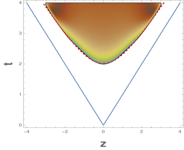
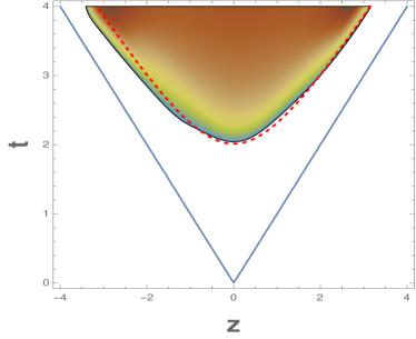
Figure 4: The largest connected spacetime region $\mathcal{R}$ in which the hydrodynamic residual $\Delta<0.15$ for a collision of narrow symmetric shocks, $w_{\pm}\,{=}\,0.075$, on the left, and asymmetric shocks, $(w_{+},w_{-})=(0.1,0.25)$, on the right. The red dotted line shows the hyperbola $(t-0.5)^{2}-z^{2}=\tau^{2}$, with $\tau=1.5$. For both asymmetric and symmetric collisions the region $\mathcal{R}$ starts at $t_{\text{hydro}}\approx 2$.

For all collisions studied, symmetric and asymmetric, with various combinations of incoming shock widths ranging from 0.35 down to 0.075, we found that the boundaries of the region $\mathcal{R}$ differ very little from one another, as illustrated in Fig. 4. At $z=0$ we find that time at which hydrodynamics first becomes valid (i.e., $\Delta<0.15$) to be essentially the same for asymmetric and symmetric collisions and given by

$$t_{\text{hydro}}\approx 2\,.$$ (61)

In the symmetric case this confirms earlier results found in Refs. Chesler:2013lia ; Chesler:2015fpa .

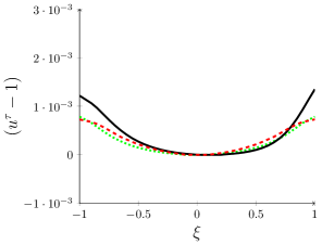
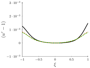
Figure 5: Left: the difference of the proper time component of the fluid velocity from unity, $u^{\tau}-1$, plotted as a function of rapidity at proper time $\tau=3$ for the asymmetric collision $(w_{+},w_{-})=(0.075,0.35)$ (black line) and the symmetric collisions $w_{\pm}=0.075$ (red dashed line) and $w_{\pm}=0.35$ (green dotted line). Right: the analogous comparison for the asymmetric collision $(w_{+},w_{-})=(0.075,0.25)$ (black line), and corresponding symmetric collisions $w_{\pm}=0.075$ (red dashed line) and $w_{\pm}=0.25$ (green dotted line). As in Ref. Chesler:2015fpa we find that $u^{\tau}\approx 1$ with a deviation of a few parts in $10^{-3}$, showing that the fluid velocity is quite well described by boost invariant flow.

For symmetric collisions, we reproduced the key results of Ref. Chesler:2015fpa : boost invariant flow (1) within the hydrodynamic region to within a precision of $\mathcal{O}(10^{-3})$, Gaussian rapidity dependence of the proper energy density (2) at fixed proper time, with the amplitude and width of this Gaussian well described by the analytic forms (5) at $\tau_{\rm init}=3$.

Turning to asymmetric collisions of shocks with differing widths, we again find that flow within the hydrodynamic region $\mathcal{R}$ is very close to ideal boost invariant flow (1), as illustrated in Fig. 5 for rapidity $\xi\in[-1,1]$. Moreover, the rapidity distribution of the proper energy density on a surface of constant proper time $\tau\gtrsim\tau_{\rm hydro}$ continues to be well approximated by a Gaussian but now with a peak which is shifted away from vanishing rapidity:

$$\epsilon(\xi,\tau)=A(w_{+},w_{-};\tau)\,e^{-\frac{1}{2}\,(\xi-\bar{\xi}(w_{+},w_{-};\tau))^{2}/\sigma(w_{+},w_{-};\tau)^{2}}\,.$$ (62)

Our results for the rapidity shift $\bar{\xi}(w_{+},w_{-};\tau)$ are shown in Fig. (6) for three examples of asymmetric collisions. To a good approximation, the width dependence of the rapidity shift has a simple factorized form for $\tau\gtrsim 2$,

$$\bar{\xi}(w_{+},w_{-};\tau)\approx\Xi\>\frac{w_{+}-w_{-}}{w_{+}+w_{-}}\,,$$ (63)

with a coefficient $\Xi\approx 0.07$ that is essentially constant for $\tau>2$.

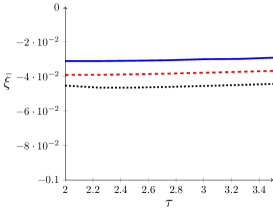
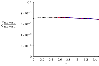
Figure 6: Left: the rapidity shift $\bar{\xi}(w_{+},w_{-};\tau)$ of the proper energy density distribution, as a function of proper time $\tau$, for asymmetric collisions with shock widths $(w_{+},w_{-})=(0.075,0.25)$ (dashed red line), $(w_{+},w_{-})=(0.1,0.25)$ (solid blue line), and $(w_{+},w_{-})=(0.075,0.35)$ (dotted black line). Right: the coefficient function $\Xi(\tau)\equiv\bar{\xi}(w_{+},w_{-};\tau)\big{(}\frac{w_{+}+w_{-}}{w_{-}-w_{+}}\big{)}$ for the same three cases.

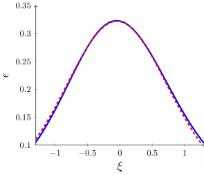
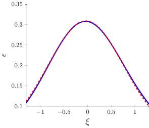
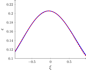
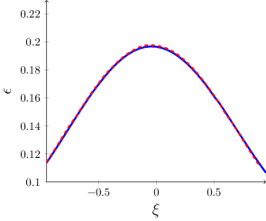
Figure 7: The proper energy density $\epsilon$ as a function of rapidity $\xi$ at constant proper time $\tau=2$ (first row) and $\tau=3$ (second row) for asymmetric collisions with $(w_{+},w_{-})=(0.075,0.35)$ (left) and $(w_{+},w_{-})=(0.075,0.25)$ (right) displayed as the solid blue curves. On each plot, the red dashed curve shows the geometric mean of the corresponding symmetric distributions shifted by $\bar{\xi}$ as given in Eq. (63). Only at $|\xi|\gtrsim 1$ is a slight deviation between the two visible.

We find that the rapidity distribution of of the proper energy density for the asymmetric collisions is well approximated by the shifted geometric mean of the corresponding symmetric collision results,

$$\epsilon(\xi,\tau;w_{+},w_{-})\approx\left[\epsilon(\xi-\bar{\xi}(w_{+},w_{-};\tau),\tau;w_{+},w_{+})\>\epsilon(\xi-\bar{\xi}(w_{+},w_{-};\tau),\tau;w_{-},w_{-})\right]^{1/2}\,.$$ (64)

The efficacy of this relation is illustrated in Fig. 7, which shows the proper energy density as a function of the rapidity $\xi$ at proper times $\tau=2$ (top) and $3$ (bottom) for the case of $(w_{+},w_{-})=(0.075,0.35)$ (left) and $(w_{+},w_{-})=(0.075,0.25)$ (right). In each plot the solid blue line shows the asymmetric collision result while the red dashed curve shows the shifted geometric mean of the corresponding symmetric collision results. For $|\xi|<1$ this model fits almost perfectly, while for $|\xi|>1$ small deviations from this simple description begin to show.

To motivate a more elaborate model which captures these deviations from the simple model (64), let

$$\langle X\rangle_{p}\equiv\left[\tfrac{1}{2}X(w_{+})^{p}+\tfrac{1}{2}X(w_{-})^{p}\right]^{1/p}$$ (65)

denote the generalized mean with power $p$ of some quantity $X$ which is observable in symmetric collisions of shocks with widths $w_{+}$ and $w_{-}$, and then define $p[X]$ as the power for which the generalized mean of symmetric collision results gives the result $X(w_{+},w_{-})$ of this observable in an asymmetric collision with shock widths $(w_{+},w_{-})$. In other words, $p[X]$ is the solution to the equation

$$\langle X\rangle_{p[X]}=X(w_{+},w_{-})\,.$$ (66)

Recall that the geometric mean is the $p\to 0$ limit of the generalized mean (65).

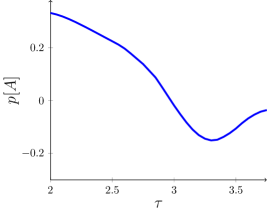
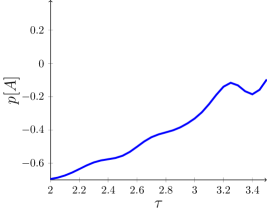
Figure 8: The exponent $p[A(\tau)]$, defined as the solution to relation (66) for the rapidity distribution amplitude $A$, as a function of proper time $\tau$, for collisions with $(w_{+},w_{-})=(0.075,0.35)$ (left) and $(w_{+},w_{-})=(0.1,0.25)$ (right).

Fig. 8 displays the resulting power $p[A(\tau)]$ for the amplitude $A$ of the distributions in rapidity of the proper energy density, as a function of proper time $\tau$, resulting from collisions with widths $(w_{+},w_{-})=(0.075,0.35)$ on the left and $(w_{+},w_{-})=(0.1,0.25)$ on the right. One sees that $p[A]$ is quite small, appearing to approach $0$ at late times. Fig. 9 directly compares the amplitude $A(\tau)$ for asymmetric collisions with the geometric mean of the corresponding symmetric collision results. For times $\tau>2$, the difference is negligible.

To construct an improved model, let

$$g_{\pm}(\xi,\tau)\equiv e^{-\frac{1}{2}\,\xi^{2}/\sigma(w_{\pm};\tau)^{2}}$$ (67)

denote the Gaussian of a symmetric collision rapidity distribution (without the corresponding amplitude). Then replace the geometric mean of the simple model (64) by a biased mean of symmetric collision Gaussians,

$$\epsilon(w_{+},w_{-};\zeta,\tau) \approx\sqrt{A(w_{+};\tau)A(w_{-};\tau)}\;g_{+}(\xi{-}\bar{\xi},\tau)^{1/2-a(w_{+},w_{-};\xi-\bar{\xi},\tau)}$$

$$\hskip 108.405pt\times g_{-}(\xi{-}\bar{\xi},\tau)^{1/2+a(w_{+},w_{-};\xi-\bar{\xi},\tau)}\,,$$ (68)

where, once again, $A(w_{\pm},\tau)$ is the amplitude of the rapidity distribution for symmetric collisions of width $w_{\pm}$, and the rapidity shift $\bar{\xi}$ is given in Eq. (63). If the bias $a(w_{+},w_{-};\xi,\tau)$ vanishes, then this form reduces to the previous simple model (64).

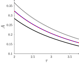
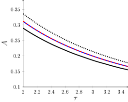
Figure 9: The amplitude $A$ (or maximum of the energy density rapidity distribution) for asymmetric collisions with $(w_{+},w_{-})=(0.075,0.35)$ (left) and $(w_{+},w_{-})=(0.1,0.25)$ (right), shown as the (middle) blue line. In each plot, the upper (dotted) line and lower (solid) line show the amplitude for the corresponding symmetric collision with wider or narrower width, respectively. In each plot, the red dashed line, overlaying the middle blue curve, shows the geometric mean of the respective symmetric collision results.

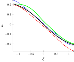
Figure 10: The bias function $a$ as a function of rapidity $\xi$, evaluated at $\tau=2$, for the cases $(w_{+},w_{-})=(0.075,0.35)$ (green line), $(w_{+},w_{-})=(0.075,0.25)$ (red dashed line), and $(w_{+},w_{-})=(0.1,0.25)$ (blue dotted line). The black line corresponds to the fitting function $f(\xi)=-\tanh(\xi)/4$.

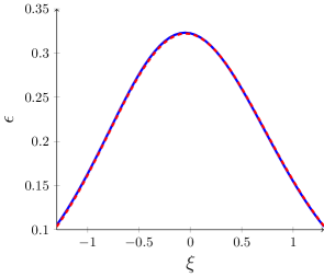
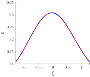
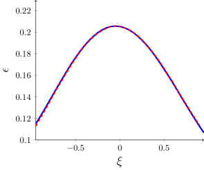
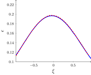
Figure 11: The proper energy density $\epsilon$ as a function of rapidity $\xi$ at constant proper time $\tau=2$ (first row) and $\tau=3$ (second row) for asymmetric collisions with $(w_{+},w_{-})=(0.075,0.35)$ (left) and $(w_{+},w_{-})=(0.075,0.25)$ (right), displayed by the solid blue curve. The overlaid red dashed curve shows the result obtained from the improved model (68), with bias function $a(\xi)=-\tfrac{1}{4}\,\tanh\xi$, and the respective Gaussian distributions for the corresponding symmetric collisions.

Fitting the improved model (68) to our numerical results, we find that the resulting bias function $a(w_{+},w_{-};\xi,\tau)$ is remarkably insensitive to the widths $(w_{+},w_{-})$ and is also constant for $\tau>2$ to quite good accuracy. Our results for $a$ are displayed in Fig. 10 for the the cases $(w_{+},w_{-})=(0.075,0.35)$, $(w_{+},w_{-})=(0.075,0.25)$, and $(w_{+},w_{-})=(0.1,0.25)$ which, as shown, differ negligibly from each other. The resulting bias function $a(\xi)$ is well described by the simple universal function

$$a(w_{+},w_{-};\xi,\tau)\approx a(\xi)\equiv-\tfrac{1}{4}\,\tanh\xi\,.$$ (69)

To show the efficacy of the improved model (68) and the improvement as compared with the simple model (64), we again compare in Fig. 11 the proper energy density rapidity distributions from asymmetric collisions along with the predictions of the above improved model (68) with bias function (69), for the same cases shown earlier in Fig. 7. As one sees, the curves are now essentially indistinguishable.

5 Discussion

The goals of this work were twofold: On the one hand by studying and quantitatively modeling asymmetric planar shock collisions via holography, we aim to help bridge the gap between descriptions of very early states of a quark gluon plasma formed during heavy ion collisions and the later hydrodynamic regime to which the system evolves. On the other hand, we also hope that a relatively didactic and detailed description of the computational techniques and software construction will be useful to others.

By studying asymmetric collisions of planar shockwaves in AdS₅, we found that the simple “universal flow” description of symmetric shock collisions, found in Ref. Chesler:2015fpa , generalizes very naturally to asymmetric shock collisions. Within the hydrodynamic regime, the fluid flow is extremely close to ideal boost invariant flow, while the proper energy density has a Gaussian rapidity dependence. Characterizing the dependence on the amplitude and widths of the initial shocks enabled the construction of a simple model for mapping initial state energy density distributions to hydrodynamic initial data, valid to leading order in transverse gradients and having potential applicability to non-central collisions of highly relativistic nuclei.

The hydrodynamization time was confirmed to be very insensitive to the widths of the colliding shocks, and dependent only on the CM frame energy density. Viewing asymmetric collisions of planar shockwaves as models for “pixels” within non-central collisions of finite sized projectiles with large aspect ratios, this result implies that the hydrodynamization time, measured in the lab frame, increases towards the fringes of the almond-shaped overlap region that forms the post-collision quark-gluon plasma. Suitably modeling the initial state transverse energy density as a function of the distance to the center of the Lorentz-contracted nuclei allows one to estimate the hydrodynamization time of different layers of the quark-gluon plasma.

Possible topics for future work include the analysis of non-local observables and entropy production during asymmetric collisions of planar shocks, explicit comparison of holographic results for localized shock collisions with our model for hydrodynamic initial data, and systematic incorporation of higher terms in an expansion in transverse gradients into this model.

Appendix A Einstein equations for planar shocks

In this section we write down explicit forms for the Einstein equations (19a)-(19g) for planar shocks. We parametrize the rescaled spatial metric $\hat{g}$ as

$$\hat{g}=\begin{pmatrix}e^{B}&0&0\\ 0&e^{B}&0\\ 0&0&e^{-2B}\end{pmatrix},$$ (70)

with a single anisotropy function $B(u,t,z)$. (Recall that $u\equiv 1/r$.) The time-space metric components $F_{x}$ and $F_{y}$ vanish due to rotational invariance in the transverse plane and, for brevity, we write just $F$ below in place of $F_{z}$ for the remaining time-space component. The resulting Einstein equations in our infalling coordinates have the schematic form:

$$\left(\partial_{r}^{2}+Q_{\Sigma}[B]\right)\Sigma =0\,,$$ (71a)

$$\left(\partial_{r}^{2}+P_{F}[B,\Sigma]\partial_{r}+Q_{F}[B,\Sigma]\right)F =S_{F}[B,\Sigma]\,,$$ (71b)

$$\left(\partial_{r}+Q_{d_{+}\Sigma}[\Sigma]\right)d_{+}\Sigma =S_{d_{+}\Sigma}[B,\Sigma,F]\,,$$ (71c)

$$\left(\partial_{r}+Q_{d_{+}B}[B,\Sigma]\right)d_{+}B =S_{d_{+}B}[B,\Sigma,F,d_{+}\Sigma]\,,$$ (71d)

$$\partial_{r}^{2}A =S_{A}[B,\Sigma,F,d_{+}\Sigma,d_{+}B]\,,$$ (71e)

$$\left(\partial_{r}+Q_{d_{+}F}[B,\Sigma]\right)d_{+}F =S_{d_{+}F}[B,\Sigma,F,d_{+}\Sigma,d_{+}B,A]\,,$$ (71f)

$$d_{+}\left(d_{+}\Sigma\right) =S_{d^{2}_{+}\Sigma}[B,\Sigma,F,d_{+}\Sigma,d_{+}B,A]\,,$$ (71g)

which specialize the general infalling form (19) to the case of planar shocks. Denoting radial derivatives with primes, $f^{\prime}\equiv\partial f/\partial r$, and $f_{,z}\equiv\partial f/\partial z$ for longitudinal derivatives, the explicit form of the various coefficient and source functions are as follows:

$$Q_{\Sigma} =\tfrac{1}{2}{B^{\prime 2}}\,,$$ (72a)

$$P_{F} =2B^{\prime}+\Sigma^{\prime}\,\Sigma^{-1}\,,$$ (72b)

$$Q_{F} =2B^{\prime\prime}+(6B^{\prime}\,\Sigma^{\prime}+4\Sigma^{\prime\prime})\,\Sigma^{-1}+3B^{\prime 2}-4\Sigma^{\prime 2}\,\Sigma^{-2}\,,$$ (72c)

$$S_{F} =2B^{\prime}_{,z}+(4\Sigma^{\prime}_{,z}+6B^{\prime}\,\Sigma_{,z})\,\Sigma^{-1}+3B_{,z}\,B^{\prime}-4\Sigma^{\prime}\,\Sigma_{,z}\,\Sigma^{-2}\,,$$ (72d)

$$Q_{d_{+}\Sigma} =2\Sigma^{\prime}\,\Sigma^{-1}\,,$$ (72e)

$$S_{d_{+}\Sigma} =-2\Sigma+\frac{e^{2B}}{12\Sigma^{3}}\bigg{\{}{}8\Sigma\big{[}F\big{(}2\Sigma^{\prime}_{,z}+F^{\prime}\,\Sigma^{\prime}\big{)}+F^{2}\,\Sigma^{\prime\prime}+F_{,z}\,\Sigma^{\prime}+\Sigma_{,{zz}}\big{]}$$

$${}+2\Sigma\,(F\,\Sigma^{\prime}+\Sigma_{,z})\big{(}8(F\,B^{\prime}+B_{,z})+F^{\prime}\big{)}-4\big{(}F\Sigma^{\prime}+\Sigma_{,z}\big{)}^{2}$$

$${}+\Sigma^{2}\Big{[}2F\big{(}4B_{,z}^{\prime}+B^{\prime}\,(7B_{,z}+4F^{\prime})+F^{\prime\prime}\big{)}+2F^{\prime}_{,z}+4B^{\prime}F_{,z}$$

$$\qquad{}+F^{2}\big{(}4B^{\prime\prime}+7B^{\prime 2}\big{)}+4B_{,z}F^{\prime}+7B_{,z}^{2}+4B_{,zz}+F^{\prime 2}\Big{]}\bigg{\}}\,,$$ (72f)

$$Q_{d_{+}B} =\tfrac{3}{2}\Sigma^{\prime}\,\Sigma^{-1}\,,$$ (72g)

$$S_{d_{+}B} =\tfrac{3}{2}B^{\prime}\,d_{+}\Sigma\,\Sigma^{-1}-\frac{e^{2B}}{6\Sigma^{4}}\bigg{\{}\Sigma^{2}\big{(}2F^{\prime}_{,z}+B^{\prime}F_{,z}+B_{,z}F^{\prime}+B_{,z}^{2}+B_{,zz}+F^{\prime 2}\big{)}$$

$${}+F\Big{[}\Sigma(4\Sigma^{\prime}_{,z}+B^{\prime}\,\Sigma_{,z}+B_{,z}\,\Sigma^{\prime}-2F^{\prime}\,\Sigma^{\prime})+2\Sigma^{2}\big{(}B^{\prime}_{,z}+B^{\prime}(B_{,z}+F^{\prime})+F^{\prime\prime}\big{)}$$

$${}-8\Sigma^{\prime}\Sigma_{,z}\Big{]}+F^{2}\Big{[}\Sigma\big{(}B^{\prime}\Sigma^{\prime}+2\Sigma^{\prime\prime}\big{)}+\Sigma^{2}\big{(}B^{\prime\prime}+B^{\prime 2}\big{)}-4\Sigma^{\prime 2}\Big{]}$$

$${}+\Sigma\big{(}B_{z}\Sigma_{,z}-4F^{\prime}\Sigma_{,z}+2F_{,z}\Sigma^{\prime}+2\Sigma_{,zz}\big{)}-4\Sigma_{,z}^{2}\bigg{\}}\,,$$ (72h)

$$S_{A} =\tfrac{3}{2}d_{+}B\,B^{\prime}-6d_{+}\Sigma\,\Sigma^{\prime}\,\Sigma^{-2}+2+\frac{e^{2B}}{4\Sigma^{4}}\bigg{\{}-8\Sigma\Big{[}F(\Sigma^{\prime}_{,z}+F^{\prime}\,\Sigma^{\prime}+F\Sigma^{\prime\prime})$$

$$\qquad{}+F\Sigma^{\prime}_{,z}+F_{,z}\,\Sigma^{\prime}+\Sigma_{,zz}+2(F\,B^{\prime}+B_{,z})(F\,\Sigma^{\prime}+\Sigma_{,z})\Big{]}+4\big{(}F\Sigma^{\prime}+\Sigma_{z}\big{)}{}^{2}$$

$${}+\Sigma^{2}\Big{[}-7(F\,B^{\prime}+B_{,z})^{2}+F^{\prime 2}-4\big{(}F\big{(}2B^{\prime}_{,z}+B^{\prime}\,F^{\prime}\big{)}+F^{2}\,B^{\prime\prime}+B^{\prime}\,F_{,z}+B_{,zz}\big{)}\Big{]}\bigg{\}}\,,$$ (72i)

$$Q_{d_{+}F} =2B^{\prime}-2\Sigma^{\prime}\,\Sigma^{-1}\,,$$ (72j)

$$S_{d_{+}F} =-2(A^{\prime}_{,z}+F\,A^{\prime\prime}+A^{\prime}\,F^{\prime})-2(B^{\prime}-\Sigma^{\prime}\,\Sigma^{-1})(FA^{\prime}+A_{,z})+A^{\prime}F^{\prime}$$

$${}-3d_{+}B\Big{[}F\,B^{\prime}+B_{,z}+2(F\Sigma^{\prime}+\Sigma_{,z})\,\Sigma^{-1}\Big{]}-2\big{(}F\,(d_{+}B)^{\prime}+(d_{+}B)_{,z}\big{)}$$

$${}+d_{+}\Sigma\,\big{(}3\Sigma F^{\prime}+4(F\Sigma^{\prime}+\Sigma_{,z})\big{)}\,\Sigma^{-2}-4\big{(}F\,(d_{+}\Sigma)^{\prime}+(d_{+}\Sigma)_{,z}\big{)}\,\Sigma^{-1}\,,$$ (72k)

$$S_{d_{+}^{2}\Sigma} =-\frac{e^{2B}}{3\Sigma^{2}}\bigg{\{}\Sigma\Big{[}FA^{\prime}_{,z}+F\big{(}A^{\prime}_{,z}+FA^{\prime\prime}+A^{\prime}F^{\prime}\big{)}+2\big{(}FA^{\prime}+A_{,z}\big{)}\big{(}FB^{\prime}+B_{,z}\big{)}$$

$${}+A^{\prime}\,F_{,z}+A_{,zz}-2d_{+}F\,(F\,B^{\prime}+B_{,z})-(d_{+}F)_{,z}-F(d_{+}F)^{\prime}\Big{]}$$

$${}+\big{(}F\Sigma^{\prime}+\Sigma_{,z}\big{)}\big{(}FA^{\prime}+A_{,z}-d_{+}F\big{)}\bigg{\}}-A^{\prime}\,d_{+}\Sigma+\tfrac{1}{2}\Sigma\,d_{+}B{}^{2}\,.$$ (72l)

The condition (24) that the apparent horizon lie at a fixed radial position $r_{h}$ has the explicit form (53). For planar shocks the horizon stationarity condition (25) becomes:

$$0 =A_{,zz}+A_{,z}\left[-F^{\prime}-2F\left(B^{\prime}-\frac{\Sigma^{\prime}}{\Sigma}\right)+2B_{,z}+\frac{\Sigma_{,z}}{\Sigma}\right]$$

$${}+\tfrac{1}{4}A\,\bigg{\{}F^{\prime 2}-2F^{\prime}_{,z}-2F^{\prime}\left(2B_{,z}+\frac{\Sigma_{,z}}{\Sigma}\right)-4F_{,z}\left(B^{\prime}-3\frac{\Sigma^{\prime}}{\Sigma}\right)+F^{2}\bigg{[}\bigg{(}B^{\prime}-\frac{4\Sigma^{\prime}}{\Sigma}\bigg{)}^{2}-\frac{6\Sigma^{\prime\prime}}{\Sigma}\bigg{]}$$

$$\qquad{}+4FF^{\prime}\left(B^{\prime}-\frac{\Sigma^{\prime}}{\Sigma}\right)-4F\left(B^{\prime}_{,z}+2B^{\prime}B_{,z}-6B_{,z}\,\frac{\Sigma^{\prime}}{\Sigma}+B^{\prime}\,\frac{\Sigma_{,z}}{\Sigma}-\frac{\Sigma^{\prime}_{,z}}{\Sigma}-2\frac{\Sigma_{,z}\Sigma^{\prime}}{\Sigma^{2}}\right)$$

$$\qquad{}+4B_{,zz}+7(B_{,z})^{2}+16B_{,z}\frac{\Sigma_{,z}}{\Sigma}+\frac{8\Sigma_{,zz}}{\Sigma}-\frac{4(\Sigma_{,z})^{2}}{\Sigma^{2}}+24\,e^{-2B}\left(\Sigma^{\prime}\,d_{+}\Sigma-\Sigma^{2}\right)\bigg{\}}$$

$${}+F_{,z}\,\bigg{(}2d_{+}B-\frac{d_{+}\Sigma}{\Sigma}\bigg{)}-\tfrac{3}{2}F^{2}\left(d_{+}B\,B^{\prime}-\frac{(d_{+}\Sigma)^{\prime}}{\Sigma}+4-\frac{2d_{+}\Sigma}{\Sigma}\left(B^{\prime}+\frac{\Sigma^{\prime}}{\Sigma}\right)\right)$$

$${}-F\,\left(\frac{3(d_{+}\Sigma)_{,z}}{\Sigma}+d_{+}B\bigg{(}B_{,z}-\frac{4\Sigma_{,z}}{\Sigma}\bigg{)}-\frac{d_{+}\Sigma}{\Sigma}\bigg{(}3F^{\prime}-2B_{,z}+\frac{2\Sigma_{,z}}{\Sigma}\bigg{)}\right)$$

$${}+\frac{e^{2B}}{4\Sigma^{2}}\left\{-6\,(d_{+}B)^{2}\,\Sigma^{4}+F^{4}\bigg{(}B^{\prime}+\frac{2\Sigma^{\prime}}{\Sigma}\bigg{)}^{2}+2F^{3}\bigg{(}B^{\prime}+\frac{2\Sigma^{\prime}}{\Sigma}\bigg{)}\bigg{(}2F^{\prime}+B_{,z}+\frac{2\Sigma_{,z}}{\Sigma}\bigg{)}\right.$$

$$\qquad{}\left.+F^{2}\bigg{(}F^{\prime 2}+4B_{,z}\,F^{\prime}+(B_{,z})^{2}+(2F^{\prime}+B_{,z})\frac{4\Sigma_{,z}}{\Sigma}+\frac{4(\Sigma_{,z})^{2}}{\Sigma^{2}}\bigg{)}\right\}.$$ (73)

Appendix B Transformation to infalling coordinates

The metric

$$ds_{\rm FG}^{2}=\tilde{\rho}^{-2}\left(-d\tilde{t}^{2}+d\tilde{\mathbf{x}}^{2}_{\bot}+d\tilde{z}^{2}+d\tilde{\rho}^{2}\right)+\tilde{\rho}^{2}\,h(\tilde{x}_{-})\,d\tilde{x}_{+}^{2}\,,$$ (74)

with $\tilde{x}_{\pm}\equiv\tilde{t}\pm\tilde{z}$, describes a single shock moving in the $+\tilde{z}$ direction using Fefferman-Graham (FG) coordinates. It gives a solution to the Einstein equations for any longitudinal profile function $h(\tilde{x}_{+})$, To construct initial data decsribing two counter-propagating shocks, we first transform a single shock solution to the infalling Eddington-Finkelstein (EF) form,

$$ds_{\rm EF}^{2}=-2dt\left[u^{-2}\,du+A\,dt+F\,dz\right]+\Sigma^{2}\left[e^{B}d\mathbf{x}_{\perp}^{2}+e^{-2B}\,dz^{2}\right]$$ (75)

with the metric functions $A$, $F$, $\Sigma$, and $B$ depending only on $t{-}z$ and the inverted radial coordinate $u\equiv 1/r$. In other words, the components $g_{uA}$ all vanish except for $g_{ut}=-u^{-2}$. We relate the FG and EF coordinates according to

$$\tilde{t}=t+u+\alpha(t{-}z,u)\,,\quad\tilde{z}=z-\gamma(t{-}z,u)\,,\quad\tilde{\rho}=u+\beta(t{-}z,u)\,,$$ (76)

along with $\tilde{\mathbf{x}}_{\bot}=\mathbf{x}_{\bot}$. Demanding that this change of coordinates yields a metric of the desired form, i.e.,

$$(g_{\rm EF})_{CD}=\frac{\partial\tilde{x}^{A}}{\partial x^{C}}\,\frac{\partial\tilde{x}^{B}}{\partial x^{D}}\,(g_{\rm FG})_{AB}\,,$$ (77)

leads to the following equations for the transformation functions,

$$0 =-\alpha^{\prime}\left(\alpha^{\prime}{+}2\right)+\beta^{\prime}\left(\beta^{\prime}{+}2\right)+\gamma^{\prime 2}+H(\beta{+}u)^{4}\left(\alpha^{\prime}{+}\gamma^{\prime}{+}1\right)^{2},$$ (78a)

$$0 =-\left(\alpha^{\prime}{+}1\right)\alpha_{,z}+\left(\beta^{\prime}{+}1\right)\beta_{,z}-\gamma^{\prime}\left(-\gamma_{,z}{+}1\right)+H(\beta{+}u)^{4}\left(\alpha^{\prime}{+}\gamma^{\prime}{+}1\right)\left(\alpha_{,z}{+}\gamma_{,z}{-}1\right),$$ (78b)

$$0 =\gamma^{\prime}\left(2\gamma_{,z}{+}1\right)+\beta^{2}/u^{2}+2\beta/u-\alpha^{\prime}-\gamma^{\prime}\,,$$ (78c)

arising from the specified values of $(g_{\rm EF})_{uu}$, $(g_{\rm EF})_{uz}$, and $(g_{\rm EF})_{ut}+(g_{\rm EF})_{uz}$, respectively. Here primes denote radial derivatives $\partial/\partial u$, and $H\equiv h\left(t-z+u+\alpha+\gamma\right)$. The dependence of the functions $H$, $\alpha$, $\beta$ and $\gamma$ on their two arguments of $t{-}z$ and $u$ is suppressed for brevity. The desired solutions to Eqs. (78) have the near-boundary behavior

$$\alpha\sim-\lambda u^{2}(1{+}\lambda u)^{-1}+O(u^{5})\,,\quad\beta\sim-\lambda u^{2}(1{+}\lambda u)^{-1}+O(u^{5})\,,\quad\gamma\sim O(u^{5})\,.$$ (79)

Following Ref. Chesler:2013lia , it is helpful to redefine $\alpha$ and $\beta$ in terms of two new functions $\delta$ and $\zeta$ via

$$\alpha=-\gamma+\beta+\delta\,,\qquad\beta=-\frac{u^{2}\zeta}{1+u\zeta}\,.$$ (80)

Inserting these expressions into equations (78) and taking appropriate linear combinations of the results leads to a pair of coupled equations for $\delta$ and $\zeta$,

$$\frac{\partial\delta}{\partial u}-\frac{u^{2}}{(1+u\zeta)^{2}}\frac{\partial\zeta}{\partial u}=0\,,\quad\frac{1}{u^{2}}\left(u^{2}\frac{\partial\zeta}{\partial u}\right)+\frac{2uH}{(1+u\zeta)^{5})}=0\,,$$ (81)

plus a single decoupled equation for $\gamma$,

$$\frac{\partial\gamma}{\partial u}-\frac{u^{2}}{(1+u\zeta)^{2}}\frac{\partial\zeta}{\partial u}+\frac{u^{4}}{2(1+u\zeta)^{2}}\left(\frac{\partial\zeta}{\partial u}\right)^{2}+\frac{u^{4}H}{2(1+u\zeta)^{6}}=0\,.$$ (82)

Alternatively, starting from the infalling form (75), it is easy to show that curves along which $r\equiv 1/u$ varies with all other coordinates held fixed are null geodesics (with $r$ as an affine parameter). Since coordinate transformations are isometries, the same curves must satisfy the geodesic equation expressed in FG coordinates, i.e.

$$\frac{d^{2}\widetilde{Y}^{A}}{dr^{2}}+\widetilde{\Gamma}^{A}_{BC}\,\frac{d\widetilde{Y}^{B}}{dr}\,\frac{d\widetilde{Y}^{C}}{dr}=0\,,$$ (83)

where $\widetilde{\Gamma}$ are the Christoffel symbols evaluated in FG coordinates. The solution $\widetilde{Y}^{A}(r)$ to this geodesic equation which begins at boundary coordinates $x^{\mu}=(t,\mathbf{x}_{\perp},z)$ with null tangent $\frac{d}{dr}\widetilde{Y}^{A}(r)=(\delta^{A}_{t}+\delta^{A}_{\rho})$ on the boundary directly gives the FG coordinates corresponding to the event with EF coordinates of $x^{M}=(t,\mathbf{x}_{\perp},z,1/r)$. Parametrizing the resulting coordinate transformation using Eq. (76), the non-trivial $t$, $z$ and $u$ components of the geodesic equation (83) lead to second order equations for the transformation functions,

$$\alpha^{\prime\prime} =-\frac{2\left(\alpha^{\prime}{+}1\right)}{u}+\frac{2(\alpha^{\prime}{+}1)(\beta^{\prime}{+}1)}{\beta{+}u}$$

$$\qquad{}+\tfrac{1}{2}\left[H^{\prime}(\beta{+}u)^{4}(\alpha^{\prime}{+}\gamma^{\prime}{+}1)^{2}+8H(\beta^{\prime}{+}1)(\beta{+}u)^{3}(\alpha^{\prime}{+}\gamma^{\prime}{+}1)\right],$$ (84a)

$$\gamma^{\prime\prime} =-\gamma^{\prime}\,\frac{2(\beta-u\beta^{\prime})}{(u(\beta+u))}-\tfrac{1}{2}\left[H^{\prime}(\beta{+}u)^{4}\left(\alpha^{\prime}{+}\gamma^{\prime}{+}1\right)^{2}+8H(\beta^{\prime}{+}1)(\beta{+}u)^{3}(\alpha^{\prime}{+}\gamma^{\prime}{+}1)\right],$$ (84b)

$$\beta^{\prime\prime} =-\frac{2}{u}\,\beta^{\prime}-\frac{2}{u}+\frac{1}{\beta}\left[H(\beta+u)^{4}(\alpha^{\prime}+\gamma^{\prime}+1)^{2}+(\alpha^{\prime}(\alpha^{\prime}+2)+\beta^{\prime 2}-\gamma^{\prime 2}-u\beta^{\prime\prime})\right].$$ (84c)

B.1 Near-boundary expansions

The transformation equations (78), with boundary conditions (79), may be solved order-by-order in $u$. If one chooses the radial shift $\lambda$ to vanish, then

$$\alpha=u^{5}\sum_{i=0}^{\infty}a_{i}\,u^{i}\,,\quad\beta=u^{5}\sum_{i=0}^{\infty}b_{i}\,u^{i}\,,\quad\gamma=u^{5}\sum_{i=0}^{\infty}g_{i}\,u^{i}\,,\quad$$ (85)

while with a non-vanishing radial shift $\lambda$ one instead has

$$\alpha=\sum_{i=1}^{\infty}u^{i+1}\lambda^{i}-\sum_{i=0}^{\infty}\>a_{i}\,u^{i+5}\>\sum_{j=-}^{\infty}\binom{4+j+i}{j}\,\lambda^{j}\,u^{j}\,,$$ (86)

$$\beta=\sum_{i=1}^{\infty}u^{i+1}\lambda^{i}+\sum_{i=0}^{\infty}\>b_{i}\,u^{i+5}\>\sum_{j=0}^{\infty}\binom{4+j+i}{j}\,\lambda^{j}\,u^{j}\,,$$ (87)

$$\gamma=\sum_{i=0}^{\infty}g_{i}\,u^{i+5}\>\sum_{j=0}^{\infty}\>\binom{4+j+i}{j}\,\lambda^{j}\,u^{j}\,.$$ (88)

For our choice of a Gaussian profile function (34), the first six orders of expansions coefficients are:

$$a_{0}=\frac{4\,e^{-\frac{z^{2}}{2w^{2}}}}{15\sqrt{2\pi}\,w}\,,$$ (89a)

$$a_{1}=\frac{11\,z\,e^{-\frac{z^{2}}{2w^{2}}}}{60\sqrt{2\pi}\,w^{3}}\,,$$ (89b)

$$a_{2}=\frac{37\,z\,(z^{2}-3w^{2})\,e^{-\frac{z^{2}}{2w^{2}}}}{2016\sqrt{2\pi}\,w^{7}}\,,$$ (89c)

$$a_{3}=\frac{768\,w^{7}e^{-\frac{z^{2}}{w^{2}}}+23\sqrt{2\pi}\,(3w^{4}-6w^{2}z^{2}+z^{4})\,e^{-\frac{z^{2}}{2w^{2}}}}{12096\pi\,w^{9}}\,,$$ (89d)

$$a_{4}=\frac{1896\,zw^{7}e^{-\frac{z^{2}}{w^{2}}}+7\sqrt{2\pi}\,z(15w^{4}-10w^{2}z^{2}+z^{4})\,e^{-\frac{z^{2}}{2w^{2}}}}{21600\pi\,w^{11}}\,,$$ (89e)

$$a_{5}=\frac{(-48456w^{9}+89736w^{7}z^{2})\,e^{-\frac{z^{2}}{w^{2}}}-67\sqrt{2\pi}\,(15w^{6}-45w^{4}z^{2}+15w^{2}z^{4}-z^{6})\,e^{-\frac{z^{2}}{2w^{2}}}}{1425600\pi\,w^{13}}\,,$$ (89f)

$$b_{0}=\frac{e^{-\frac{z^{2}}{2w^{2}}}}{6\sqrt{2\pi}\,w}\,,$$ (89g)

$$b_{1}=\frac{ze^{-\frac{z^{2}}{2w^{2}}}}{10\sqrt{2\pi}\,w^{3}}\,,$$ (89h)

$$b_{2}=-\frac{(w^{2}-z^{2})\,e^{-\frac{z^{2}}{2w^{2}}}}{30\sqrt{2\pi}\,w^{5}}\,,$$ (89i)

$$b_{3}=-\frac{z(3w^{2}-z^{2})\,e^{-\frac{z^{2}}{2w^{2}}}}{126\sqrt{2\pi}\,w^{7}}\,,$$ (89j)

$$b_{4}=\frac{116w^{7}\,e^{-\frac{z^{2}}{w^{2}}}+3\sqrt{2\pi}(3w^{4}-6w^{2}z^{2}+z^{4})\,e^{-\frac{z^{2}}{2w^{2}}}}{4032\pi\,w^{9}}\,,$$ (89k)

$$b_{5}=\frac{312z\,w^{7}\,e^{-\frac{z^{2}}{w^{2}}}+\sqrt{2\pi}z\,(15w^{4}-10w^{2}z^{2}+z^{4})e^{\frac{z^{2}}{2w^{2}}}}{8640\pi\,w^{11}}\,,$$ (89l)

$$g_{0}=-\frac{e^{-\frac{z^{2}}{2w^{2}}}}{5\sqrt{2\pi}\,w}\,,$$ (89m)

$$g_{1}=-\frac{3z\,e^{-\frac{z^{2}}{2w^{2}}}}{20\sqrt{2\pi}\,w^{3}}\,,$$ (89n)

$$g_{2}=\frac{5(w^{2}-z^{2})\,e^{-\frac{z^{2}}{2w^{2}}}}{84\sqrt{2\pi}\,w^{5}}\,,$$ (89o)

$$g_{3}=\frac{-11z(z^{2}-3w^{2})\,e^{-\frac{z^{2}}{2w^{2}}}}{672\sqrt{2\pi}\,w^{7}}\,,$$ (89p)

$$g_{4}=\frac{-32w^{7}\,e^{-\frac{z^{2}}{w^{2}}}-\sqrt{2\pi}(3w^{4}-6w^{2}z^{2}+z^{4})\,e^{-\frac{z^{2}}{2w^{2}}}}{576\pi\,w^{9}}\,,$$ (89q)

$$g_{5}=\frac{-3408z\,w^{7}\,e^{-\frac{z^{2}}{w^{2}}}-13\sqrt{2\pi}\,z\,(15w^{4}-10w^{2}z^{2}+z^{4})\,e^{-\frac{z^{2}}{2w^{2}}}}{43200\pi\,w^{11}}\,.$$ (89r)

Inserting these expansions into expression (37) for the metric anisotropy function yields its near boundary expansion, $B\sim\sum_{i=4}^{\infty}B_{i}\,u^{i}$, with

$$B_{4} =-\frac{e^{-\frac{z^{2}}{2w^{2}}}}{3\sqrt{2\pi}\,w}\,,$$ (90a)

$$B_{5} =\frac{e^{-\frac{z^{2}}{2w^{2}}}\left(20\lambda\,w^{2}-3z\right)}{15\sqrt{2\pi}\,w^{3}}\,,$$ (90b)

$$B_{6} =\frac{e^{-\frac{z^{2}}{2w^{2}}}\left(-50\lambda^{2}\,w^{4}+w^{2}\,(15\lambda\,z+1)-z^{2}\right)}{15\sqrt{2\pi}\,w^{5}}\,,$$ (90c)

$$B_{7} =\frac{e^{-\frac{z^{2}}{2w^{2}}}\left(2100\lambda^{3}\,w^{6}-63\lambda\,w^{4}\,(15\lambda\,z+2)+3w^{2}\,z\,(42\lambda\,z+5)-5z^{3}\right)}{315\sqrt{2\pi}\,w^{7}}\,,$$ (90d)

$$B_{8} =\frac{e^{-\frac{z^{2}}{2w^{2}}}}{10080\pi\,w^{9}}\Big{[}\sqrt{2\pi}\,\big{(}-58800\lambda^{4}\,w^{8}+7056\lambda^{2}\,w^{6}\,(5\lambda\,z+1)-3w^{4}\,(2352\lambda^{2}\,z^{2}$$

$$\qquad\qquad{}+560\lambda\,z+15)+10w^{2}\,z^{2}\,(56\lambda\,z+9)-15z^{4}\big{)}-280\,e^{-\frac{z^{2}}{2w^{2}}}\,w^{7}\Big{]}\,,$$ (90e)

$$B_{9} =\frac{e^{-\frac{z^{2}}{2w^{2}}}}{30240\pi\,w^{11}}\Big{[}\sqrt{2\pi}\,(282240\lambda^{5}\,w^{10}-14112\lambda^{3}\,w^{8}(15\lambda\,z+4)$$

$$\qquad\qquad{}+72\lambda\,w^{6}(784\lambda^{2}\,z^{2}+280\lambda\,z+15)-15w^{4}\,z\,(448\lambda^{2}\,z^{2}+144\lambda\,z+7)$$

$$\qquad\qquad{}+10w^{2}\,z^{3}\,(36\lambda\,z+7)-7z^{5})+1120\,e^{-\frac{z^{2}}{2w^{2}}}\,(6\lambda\,w^{9}-w^{7}\,z)\Big{]}\,,$$ (90f)

$$B_{10} =\frac{e^{-\frac{z^{2}}{2w^{2}}}}{453600\pi\,w^{13}}\Big{[}\sqrt{2\pi}\,\Big{(}-6350400\lambda^{6}\,w^{12}+1905120\lambda^{4}\,w^{10}\,(3\lambda\,z+1)$$

$$\qquad\qquad{}-1620\lambda^{2}w^{8}\,(1176\lambda^{2}\,z^{2}+560\lambda\,z+45)$$

$$\qquad\qquad{}+15w^{6}\,(20160\lambda^{3}\,z^{3}+9720\lambda^{2}\,z^{2}+945\lambda\,z+14)$$

$$\qquad\qquad{}-90w^{4}\,z^{2}\,(270\lambda^{2}\,z^{2}+105\lambda\,z+7)+105w^{2}\,z^{4}\,(9\lambda\,z+2)-14z^{6}\Big{)}$$

$$\qquad\qquad{}-84\,e^{-\frac{z^{2}}{2w^{2}}}\,w^{7}\,(5400\lambda^{2}\,w^{4}-4w^{2}\,(450\lambda\,z+19)+137z^{2})\Big{]}\,.$$ (90g)

Appendix C Pseudo-spectral methods

Pseudo-spectral methods are a class of mean weighted residual approximation techniques. These methods provide highly efficient techniques for constructing accurate numerical approximations to linear differential equations of the form

$$Lf=g\,,$$ (91)

with $L$ being a linear differential operator. One approximates the solution $f$ by a linear combination of a finite set of of basis functions, $f^{(N)}=\sum_{m=0}^{N-1}\>c_{m}\,\phi_{m}$, and defines the residual

$$R^{(N)}\equiv Lf^{(N)}-g\,.$$ (92)

Given some scalar product $(\cdot,\cdot)$ for the function space in which the basis functions $\phi_{m}$ reside, and a chosen sequence $\{\xi_{m}\}$ of test functions, one solves for the coefficients $\{c_{m}\}$ of the spectral approximation $f^{(N)}$ by demanding that the residual vanish on these test functions,

$$\left(\xi_{m},R^{(N)}\right)=0\,,$$ (93)

for $m=0,{\cdots},N{-}1$. Different weighted residual methods are distinguished by the choice of the test functions. So-called “pseudo-spectral” or “collocation” methods are a subclass of mean weighted residual algorithms in which one chooses the test functions to have point support. In, for example, one dimensional problems one chooses

$$\xi_{m}=\delta(x-x_{m})\,,$$ (94)

for some selected set of points $\{x_{m}\}$. In other words, in pseudo-spectral approximations, one demands that the residual vanish identically on some discrete set of grid points distributed across the computational domain. For a given basis set $\{\phi_{m}\}$, $m=0,{\cdots},N{-}1$, there is a corresponding optimal choice of grid $\{x_{m}\}$, $m=0,{\cdots},N{-}1$, namely the abcissas of a Gaussian quadrature integration scheme associated with this basis set Boyd:Spectral . Given a choice of $N$ basis functions $\{\phi_{m}\}$ and associated spectral grid $\{x_{m}\}$, it is convenient to define “cardinal functions” $\{C_{m}\}$ which are uniquely defined as linear combinations of these basis functions which take the value 1 on a given grid point while vanishing on all other points,

$$C_{m}(x_{n})=\delta_{mn}\,,\qquad m,n=0,{\cdots},N{-}1\,.$$ (95)

The original spectral approximation $f^{(N)}=\sum_{m=0}^{N-1}c_{m}\,\phi_{m}$ is then exactly equivalent to a linear combination of cardinal functions,

$$f^{(N)}=\sum_{m=0}^{N-1}\>f_{m}\,C_{m}\,,$$ (96)

in which each coefficient is the value of the function approximation on a given grid point, $f_{m}\equiv f^{(N)}(x_{m})$.

For one dimensional problems on a finite interval, the most commonly used basis functions are Chebyshev polynomials. There are actually two corresponding sets of optimal spectral grids differing in whether the endpoints of the interval are themselves gridpoints. It is easiest to deal with boundary conditions when endpoints are included in the spectral grid in which case, for the interval $[-1,1]$, the appropriate $N{+}1$ point grid consists of the points

$$x_{m}=\cos(m\pi/N)\,,\qquad m=0,{\cdots},N\,.$$ (97)

This is sometimes referred to as a Chebyshev-Gauss-Lobatto grid.

For problems on a periodic interval, a truncated Fourier series provides the most useful spectral approximation. In this case, an appropriate $2N$ point spectral grid consists of $2N$ evenly spaced points around the periodic interval. So, for the interval $[0,2\pi]$, one may use

$$x_{m}=\pi\,m/N\,,\qquad m=0,{\cdots},2N{-}1\,.$$ (98)

If the differential equation of interest (91) involves an $M$-th order differential operator, $L=\sum_{k=0}^{M}\>p_{k}(x)\frac{d^{k}}{dx^{k}}$, then computing the values of the residual $R$ on all grid points, using the cardinal representation (96), requires the evaluation of up to $M$-th order derivatives of each cardinal function at every point on the grid. This computation need only be performed once, and defines a set of “spectral differentiation matrices” with components

$$(D^{(N)}_{k})_{mn}\equiv\frac{d^{k}C_{n}(x_{m})}{dx^{k}}\,,\qquad m,n=0,{\cdots},N{-}1\,.$$ (99)

Given these matrices, the application of the differential operator $L$ to the spectral approximation of some function reduces to the application of the finite matrix $L^{(N)}\equiv\|L^{(N)}_{mn}\|$, with

$$L^{(N)}_{mn}=\sum_{k=0}^{M}\>p_{k}(x_{m})\,(D^{(N)}_{k})_{mn}\,,\qquad m,n=0,{\cdots},N{-}1\,,$$ (100)

to the vector of function values on the spectral grid, $(Lf^{(N)})(x_{m})=\sum_{n}L^{(N)}_{mn}\,f_{n}$. Solving for (the spectral approximation to) the solution of the differential equation (91) then reduces to the standard algebraic problem of solving a finite system of linear equations.

C.1 Explicit expressions

Analytic expressions for cardinal functions and differential matrix components, for many different sets of basis functions, may be found in appendix F of Ref. Boyd:Spectral . For a Chebyshev basis and the Chebyshev-Gauss-Lobatto grid (97), cardinal functions satisfying (95) are given by

$$C_{j}(x)=(-1)^{j+1}\frac{\left(1-x^{2}\right)}{c_{j}\,N^{2}(x-x_{j})}\,\frac{dT_{N}(x)}{dx}\,,$$ (101)

where $T_{k}(x)$ denote Chebyshev polynomials of the first kind and $c_{j}\equiv 1$ for $0<j<N$ while $c_{0}=c_{N}\equiv 2$. The interior grid points lie at extrema of $T_{N}(x)$. Derivatives of these cardinal functions, evaluated on the Gauss-Lobatto grid, can be evaluated explicitly. For the first derivative one finds Boyd:Spectral

$$(D^{(N+1)}_{1})_{mn}=\frac{dC_{n}}{dx}\bigg{|}_{x=x_{m}}=\begin{cases}\tfrac{1}{6}(1+2N^{2})\,,&m=n=0;\\ -\tfrac{1}{6}(1+2N^{2})\,,&m=n=N;\\ -\tfrac{1}{2}\,x_{n}/(1-x_{n}^{2})\,,&m=n\mbox{ with }0<n<N;\\ (-1)^{m+n}c_{m}/[c_{n}(x_{m}-x_{n})]\,,&m\neq n\,.\end{cases}$$ (102)

Higher derivatives are obtained by taking powers of this matrix, $D^{(N+1)}_{k}=(D^{(N+1)}_{1})^{k}$.

For the Fourier grid with endpoint (98), cardinal functions can be expressed as

$$C_{j}(x)=\frac{1}{2N}\,\sin[N(x-x_{j})]\cot[\tfrac{1}{2}(x-x_{j})]\,,$$ (103)

and the first two differentiation matrices are given by

$$(D^{(2N)}_{1})_{mn}\equiv\frac{dC_{n}}{dx}\bigg{|}_{x=x_{m}} =\begin{cases}0\,&m=n;\\ \frac{1}{2}(-1)^{i+j}\cot\left[\frac{1}{2}\left(x_{i}-x_{j}\right)\right]\,,&m\neq n,\end{cases}$$ (104)

$$(D^{(2N)}_{2})_{mn}\equiv\frac{d^{2}C_{j}}{dx^{2}}\bigg{|}_{x=x_{i}} =\begin{cases}-\tfrac{1}{6}(1+2N^{2})\,,&m=n;\\ \tfrac{1}{2}(-1)^{i+j+1}\csc^{2}\left[\frac{1}{2}(x_{i}-x_{j})\right]\,,&m\neq n.\end{cases}$$ (105)

A linear transformation, $y=ax+b$, may be used to convert the above expressions into forms appropriate for arbitrary finite intervals.

C.2 Domain decomposition

The error in an $N$-term spectral approximation to some function $u$ decreases exponentially with increasing $N$, provided $u$ satisfies appropriate analyticity conditions Boyd:Spectral . In practice, this desirable behavior only holds as long as there is negligible round-off error from finite precision numerical arithmetic. Unfortunately, differentiation matrices become increasingly ill-conditioned as $N$ increases and this leads to progressively worsening numerical errors in the eventual solution of the linear system. Moreover, with Chebyshev grids, the spacing between grid points is non-uniform and near the endpoints of the interval the grid spacing decreases as $1/N^{2}$. This rapid decrease of grid spacing can lead to short wavelength (so-called ‘CFL’) instabilities in time evolution problems.

These difficulties can be alleviated by partitioning the computational domain into multiple subdomains, inside each of which one constructs an independent spectral approximation. This is known as domain decomposition. In effect, one solves the differential equation of interest independently in each subdomain with boundary conditions which enforce appropriate continuity conditions connecting adjoining subdomains. Differentiation matrices for the entire domain become block-diagonal.

For a one dimensional problem, if one partitions the full domain into $M$ subdomains, and uses an $N$-point Chebyshev grid containing endpoints within each subdomain, then each interior subdomain boundary will appear twice in the resulting complete list of grid points (46). For a second order differential equation, before solving the resulting linear system, $L^{(MN)}\,f^{(MN)}=g^{(MN)}$, one simply replaces each pair of rows which represent the same interior subdomain boundary by a near pair of linear equations which encode continuity of the function,

$$f^{(MN)}_{i,N-1}-f^{(MN)}_{i+1,0}=0\,,$$ (106)

and of its first derivative,

$$\sum_{k=0}^{N-1}\>(D^{(N)}_{1})_{N-1,k}\,f^{(MN)}_{i,k}-(D^{(N)}_{1})_{0,k}\,f^{(MN)}_{i+1,k}=0\,.$$ (107)

For further detail refer to Ref. Boyd:Spectral .

Appendix D Filtering

D.1 Longitudinal filter

Numerically filtering the propagating data, namely the functions $\{B,a,f,\lambda\}$, to remove small amplitude noise, specifically cutoff-scale rapid variations in the longitudinal direction, is essential to achieve stable time evolution with low background energy density, especially for narrow shock collisions where a very fine longitudinal grid is required. The reasons behind this, involving spectral blocking in non-linear equations, are discussed in Refs. Chesler:2013lia ; Boyd:Spectral .

Such filtering must be applied carefully. To maintain consistency of the solution of the nested set of Einstein equations (19), we only filter at the end of each time step, not within RK4 substeps and not in between solutions of the nested radial differential equations.

There are many ways to implement a low-pass filter. For our periodic functions of $z$, we use a smooth multiplicative filter in $k$-space. A cardinal function representation using the uniform grid (98) and Fourier cardinal functions (103), $\phi(z)=\sum_{j=0}^{2N-1}\>\phi_{j}\,C_{j}(z)$, is exactly equivalent to a truncated Fourier series,

$$\phi(z)=\sum_{k=-N}^{N}\>\tilde{\phi}_{k}\,e^{ikz}\,.$$ (108)

with

$$\tilde{\phi}_{k}\equiv\frac{(1{-}\tfrac{1}{2}\delta_{|k|}^{N})}{2N}\>\sum_{j=0}^{2N-1}\phi(\pi j/N)\,e^{-{2\pi ijk}/N}\,.$$ (109)

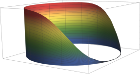
Figure 12: Visualization of our low-pass Fourier filter for periodic functions. Modes with wavevector $|k|/N\gtrsim\frac{2}{3}$ are suppressed. The filter width $\delta$ is chosen to be $1/2$.

We suppress the amplitude of modes with large $|k|$ by multiplying the Fourier coefficients $\{\tilde{\phi}_{k}\}$ by the filter function

$$\widetilde{F}(k)\equiv\frac{1}{2}\left(1-\mathrm{erf}\left[\frac{2\pi}{\delta}\left(\frac{|k|}{N}-\Lambda\right)\right]\right).$$ (110)

The parameter $\Lambda$ is the fractional bandwidth of the filter while $N\delta/(2\pi)$ is the characteristic width in wavevectors of the filter roll-off. We chose to use $\Lambda=2/3$ and $\delta=1/2$. Transforming back to real space produces the smoothed function

$$\overline{\phi}(z)\equiv\sum_{k=-N}^{N}\>\widetilde{F}(k)\,\tilde{\phi}_{k}\,e^{ikz}\,.$$ (111)

In practice, it is convenient to compute the real-space form of this filter by combining expressions (109) and (111), yielding a convolution matrix which is computed once, and then applied directly to function values on the longitudinal grid to yield filtered functions,

$$\overline{\phi}(z_{m})=\sum_{n=0}^{2N-1}\>F_{n-m}\,\phi(z_{n})\,.$$ (112)

D.2 Radial filter

After transforming single shock solutions to infalling coordinates, as described in Appendix B, we found that moderately high derivatives of the resulting anisotropy function, such as $\partial_{u}^{3}\partial_{z}^{3}b(u,z,t_{0})$, after the longitudinal filtering as just described, would still show visible noise with rapid radial and longitudinal variation. Such noise grows and becomes problematic upon time evolution. To suppress such artifacts in the initial data, we perform radial filtering on the initial anisotropy function in a matter designed to suppress radial noise near the boundary while simultaneously ensuring the correct near boundary asymptotic behavior.

We do this by first constructing, analytically, the near boundary expansion of the transformation functions solving Eqs. (39)–(40c), and thence the resulting metric anisotropy function $B(u,z,t_{0})$ via Eq. (37) [or equivalently the rescaled function $b(u,z,t_{0})$ defined in Eq. (55a)]. Explicit expressions for these near-boundary expansions appeared in Appendix B.1. Let $b^{(K)}(u,z,t_{0})$ denote the $K$-term partial sum of the near-boundary expansion for the rescaled anisotropy function $b(u,z,t_{0})$. We define a correction function $\Delta^{(K)}(u,z)$ by the condition that

$$\left(\tfrac{\partial}{\partial u}\right)^{m}\left[b(u,z,t_{0})+\Delta^{(K)}(u,z)\right]\Big{|}_{u=0}=\left(\tfrac{\partial}{\partial u}\right)^{m}b^{(K)}(u,z,t_{0})\Big{|}_{u=0}\,,$$ (113)

for $m=0,{\cdots},K{-}1$, while simultaneously requiring that $\Delta^{(K)}(u,z)$, evaluated on the radial grid, is only non-zero on the first $K$ radial grid points closest to the boundary. On the left side of condition (113), the radial derivatives are evaluated using the spectral derivative matrix $D_{u}$ applied to the list of values of $b$ and $\Delta^{(K)}$ on the radial grid. These conditions uniquely determine the correction function $\Delta^{(K)}$ (represented on the spectral grid). The corrected function $b_{\rm improved}\equiv b+\Delta^{(K)}$ coincides with the input function $b$ away from the boundary (by more than $K$ grid points), while having corrected values of radial derivatives up through order $K{-}1$ at the boundary. Choosing $K=7$, we find that this procedure is effective in suppressing numerical noise in initial data up to quite high orders of derivatives in both radial and longitudinal directions. Unlike a conventional filter, the effect of this procedure is restricted to a small region near the boundary.

Appendix E Runge-Kutta methods

Given a first order differential equation for some $\mathbb{R}^{k}$-valued function $\Phi(t)$,

$$\frac{d}{dt}\,\Phi(t)=F(t,\Phi(t))\,,$$ (114)

with initial condition $\Phi(t_{0})=\Phi_{0}$, the standard fourth order Runge-Kutta (RK4) algorithm iteratively constructs an approximate solution $\tilde{\Phi}$ at times $t_{n}\equiv t_{n-1}+\delta t$, via the recursion relation

$$\tilde{\Phi}(t_{n+1};\delta t)\equiv\tilde{\Phi}(t_{n})+\delta t\sum_{j=1}^{4}\>b_{j}\,K_{j}(t_{n})\,,$$ (115)

where

$$K_{j}(t_{n})\equiv F\big{(}t_{n}+\alpha_{j}\,\delta t,\,\tilde{\Phi}(t_{n})+\alpha_{j}\,\delta t\,K_{j-1}(t_{n})\big{)}\,,$$ (116)

with $\tilde{\Phi}(t_{0};\delta t)=\Phi_{0}$. The coefficient vectors defining the RK4 “substeps” are given by

$$\alpha=\left(0,\tfrac{1}{2},\tfrac{1}{2},1\right),\qquad b=\left(\tfrac{1}{6},\tfrac{1}{3},\tfrac{1}{3},\tfrac{1}{6}\right).$$ (117)

To convert this method to an adaptive stepsize integration method, one needs a local error estimation, i.e., some estimate of the difference between $\tilde{\Phi}(t_{n})$ and the desired solution $\Phi(t_{n})$, assuming that $\tilde{\Phi}(t_{n-1})$ is correct, together with an algorighm for decreasing or increasing the time step $\delta t$ based on this error estimate. The easiest way to achieve this is to compare the results of performing a single RK4 step with timestep $\delta t$ versus two RK4 steps with timestep $\delta t/2$. The latter (more time consuming) calcuation will suffer from less error due to timestep discretization and, if $\delta t$ is sufficiently small, this difference will be a decent approximation to the deviation from the true solution. We define

$$\text{err}(t{+}\delta t)=\big{|}\tilde{\Phi}(t{+}\delta t;\delta t)-\tilde{\Phi}(t{+}\delta t;\delta t/2)\big{|},$$ (118)

given a common starting value at time $t$. For the choice of norm, we use an $L^{\infty}$ norm, or the maximum over all components of $\tilde{\Phi}$. If the goal of the numerical calculation is to achieve a relative precision of $10^{-a}$, then we adjust the time step according to

$$\delta t_{n+1}=\delta t_{n}\bigg{(}\frac{10^{-a}}{\text{err}}\bigg{)}^{1/4}.$$ (119)

The “learning rate” of this adaptive algorithm is governed by the exponent ${1}/{4}$ in this rule. This value reflects the fact that in the basic RK4 method, the error scales as $(\delta t)^{4}$ for sufficiently small timestep $\delta t$. In our code we did not impose minimum or maximum step sizes. And in our specific application of transformation to infalling coordinates, when starting with an initial step size of $\delta u=0.0001$ it turned out to be sufficient to update the step size using Eq. (119) and always advance directly to the next slice without further adjustments. More generally, it can be necessary to reject a trial step and repeat the the calculation with a smaller step size if the initial error exceeds the desired limit.

References

- (1) P. M. Chesler, N. Kilbertus and W. van der Schee, Universal hydrodynamic flow in holographic planar shock collisions, J. High Energy Phys. 1511 (2015) 135, arXiv:1507.02548 [hep-th].
- (2) P. M. Chesler and L. G. Yaffe, Numerical solution of gravitational dynamics in asymptotically anti-de Sitter spacetimes, J. High Energy Phys. 1407 (2014) 086 arXiv:1309.1439
- (3) P. M. Chesler, L. G. Yaffe, Holography and colliding gravitational shock waves in asymptotically AdS5 spacetime, DOI: 10.1103/PhysRevLett.106.021601 arXiv:1011.3562 [hep-th]
- (4) M. P. Heller, D. Mateos, W. van der Schee and D. Trancanelli, Strong coupling isotropization of non-Abelian plasmas simplified, Phys. Rev. Lett. 108 (2012) 191601, arXiv:1202.098 [hep-th].
- (5) M. P. Heller, R. A. Janik and P. Witaszczyk, A numerical relativity approach to the initial value problem in asymptotically Anti-de Sitter spacetime for plasma thermalization - an ADM formulation, Phys. Rev. D 85 (2012) 126002, arXiv:1203.0755 [hep-th].
- (6) J. Casalderrey-Solana, M. P. Heller, D. Mateos and W. van der Schee, From full stopping to transparency in a holographic model of heavy ion collisions, Phys. Rev. Lett. 111 (2013) 181601, arXiv:1305.4919 [hep-th].
- (7) A. Buchel, M. P. Heller and R. C. Myers, Equilibration rates in a strongly coupled nonconformal quark-gluon plasma, Phys. Rev. Lett. 114 (2015) no.25, 251601, arXiv:1503.07114 [hep-th].
- (8) P. M. Chesler and L. G. Yaffe, Holography and off-center collisions of localized shock waves, J. High Energy Phys. 1510 (2015) 070 arXiv:1501.04644
- (9) W. van der Schee, P. Romatschke, S. Pratt, A fully dynamical simulation of central nuclear collisions Phys. Rev. D 111 (2013) 222302, arXiv:1307.2539 [hep-th]
- (10) W. van der Schee, B. Schenke, Rapidity dependence in holographic heavy ion collisions Phys. Rev. D C 92 (2015) 064907, arXiv:1507.08195 [hep-th]
- (11) J. Casalderrey-Solana, D. Mateos, W. van der Schee, M. Trianae, Holographic heavy ion collisions with baryon charge J. High Energy Phys. 1609 (2015) 108 arXiv:1607.05273 [hep-th]
- (12) C. Ecker, D. Grumiller, P. Stanzer, S. A. Stricker, W. van der Schee, Exploring nonlocal observables in shock wave collisions J. High Energy Phys. 1611 (2016) 054, arXiv:1609.03676 [hep-th]
- (13) P. M. Chesler, Colliding shock waves and hydrodynamics in small systems Phys. Rev. Lett 115 (2015) 241602, arXiv:1506.02209 [hep-th]
- (14) M. Attems, J. Casalderrey-Solana, D. Mateos, D. Santos-Oliván, C. F. Sopuerta, M. Triana, M. Zilhão, Holographic collisions in non-conformal theories J. High Energy Phys. 1701 (2016) 026, arXiv:1604.06439 [hep-th]
- (15) P. M. Chesler, How big are the smallest drops of quark-gluon plasma? J. High Energy Phys. 1603 (2016) 146, arXiv:1601.01583 [hep-th]
- (16) J. F. Fuini and L. G. Yaffe, Far-from-equilibrium dynamics of a strongly coupled non-Abelian plasma with non-zero charge density or external magnetic field, J. High Energy Phys. 1507 (2015) 116, arXiv:1503.07148 [hep-th].
- (17) A. Buchel, J. T. Liu and A. O. Starinets, Coupling constant dependence of the shear viscosity in N=4 supersymmetric Yang-Mills theory, Nucl. Phys. B 707 (2005) 56, arXiv:0406264 [hep-th].
- (18) S. Waeber and A. Schäfer, Studying a charged quark gluon plasma via holography and higher derivative corrections, J. High Energy Phys. 1807 (2018) 069, arXiv:1804.01912 [hep-th].
- (19) H. Bondi, Gravitational waves in general relativity, Nature 186 (1960) no.4724, 535.
- (20) R. K. Sachs, Gravitational waves in general relativity. 8. Waves in asymptotically flat space-times, Proc. Roy. Soc. Lond. A 270 (1962) 103.
- (21) J. P. Boyd, Chebyshev and Fourier Spectral Methods (Revised), Dover Books on Mathematics, Dover Publications, 2001
- (22) P. Arnold, P. Romatschke and W. van der Schee, ‘‘Absence of a local rest frame in far from equilibrium quantum matter,’’ JHEP 1410, 110 (2014) arXiv:1408.2518 [hep-th].
- (23) R. A. Janik, R. Peschanski Asymptotic perfect fluid dynamics as a consequence of AdS/CFT, Phys. Rev. D 73 (2006) 045013, arXiv:hep-th/0512162