Spin transport and Spin Tunnelling Magneto-Resistance (STMR) of F$|$NCSC$|$F spin valve

Abstract

In this work, we study the spin transport at the Ferromagnet$|$Noncentrosymmetric Superconductor (F$|$NCSC) junction of a Ferromagnet$|$Noncentrosymmetric Superconductor$|$Ferromagnet (F$|$NCSC$|$F) spin valve. We investigate the Tunnelling Spin-Conductance (TSC), spin current and Spin Tunnelling Magneto-Resistance (STMR), and their dependence on various important parameters like Rashba Spin-Orbit Coupling (RSOC), strength and orientation of magnetization, an external in-plane magnetic field, barrier strength and a significant Fermi Wavevector Mismatch (FWM) at the ferromagnetic and superconducting regions. The study has been carried out for different singlet-triplet mixing of the NCSC gap parameter. We develop Bogoliubov-de Gennes (BdG) Hamiltonian and use the extended Blonder - Tinkham - Klapwijk (BTK) approach along with the scattering matrix formalism to calculate the scattering coefficients. Our results strongly suggest that the TSC is highly dependent on RSOC, magnetization strength and its orientation, and singlet-triplet mixing of the gap parameter. It is observed that NCSC with moderate RSOC shows maximum conductance for a partially opaque barrier in presence of low external magnetic field. For a strongly opaque barrier and a nearly transparent barrier a moderate value and a low value of field respectively are found to be suitable. Moreover, NCSC with large singlet component is appeared to be useful. In addition, for NCSC with large RSOC and low magnetization strength, a giant STMR ($\%$) is observed. We have also seen that the spin current is strongly magnetization orientation dependent. With the increase in bias voltage spin current increases in transverse direction, but the component along the direction of flow is almost independent.

I Introduction

Spintronic devices, such as Spin Valves (SVs) or Magnetic Tunnelling Junctions (MTJs) have received a lot of attention over the years due to the significant progress in fabrication techniques. Traditional MTJs are composed of two ferromagnets in close proximity, normally separated by an insulator or a normal metal. When a current is allowed to flow, it interact with the exchange field of the first ferromagnet and induces a polarization in the spin degrees of freedom. The second ferromagnet is introduced as spin detector, where spin current is measured johnson ; jedema ; wolf ; casanova ; chung . The spin transport properties in these SVs are controlled mainly by the charge current, the relative orientation of the magnetization components and the external magnetic field. Moreover, depending upon the orientation of the magnetization i.e. parallel or anti parallel to the ferromagnetic regions, these hybrid structures display Giant Magneto-Resistance (GMR) effect binasch ; baibich ; parkin ; chappert and hence have a great potential to be used as a non volatile magnetic memories, sensors for harddisk drives etc.

Over the last two decades, the interplay between ferromagnetic and superconducting order potentially enhances the interest in exploring Ferromagnet$|$Superconductor (F$|$S) hybrid structures for low temperature spintronic applications eschrig1 ; eschrig2 ; zutic ; buzdin ; blamire ; bergeret ; kadigrobov ; golubov ; zhu11 ; petrashov ; flokstra ; slonczewski ; berger ; halterman1 ; halterman2 . The discovery of phenomena like proximity effect zutic ; buzdin ; petrashov ; kadigrobov , long distance transport of magnetization zutic ; buzdin ; petrashov ; kadigrobov , spin injection flokstra , Spin Transfer Torque (STT) slonczewski ; berger , and triplet correlation halterman1 ; halterman2 in F$|$S hybrid structures boosted up the superconducting spintronics research. Moreover, introduction of superconductor as a spacer in SVs provides the following advantages: (1) Superconducting spintronics devices can intricate strong proximity effect between the superconductor and the ferromagnet zutic ; buzdin ; petrashov ; kadigrobov , hence it gains a lot of interest from application point of view. (2) Superconducting SVs also reduce the consumption of energy and hence can be highly useful to fabricate ultra fast cryogenic magnetic memory devices golubov ; zhu11 . (3) Furthermore, unconventional superconductors can also support polarized current bergeret ; blamire ; eschrig1 ; eschrig2 and hence it can be the potential candidate for superconducting spintronic devices.

Traditionally, conventional superconductors are introduced as a spacer in MTJs. However, conventional superconductors are highly irreconcilable with ferromagnetism as the exchange coupling of a ferromagnet destroy the singlet pairing of the Cooper pairs bardeen . On the other hand, superconductivity results from the triplet pairing of the Cooper pairs can coexist with ferromagnetism and hence they are the prime candidates of F$|$S$|$F SVs. From the point of view of Cooper pairs, two symmetries play most pivotal role: the symmetry of centre of inversion and the symmetry of time reversal. In absence of any of them the pairing can appear in an unconventional form. Over the last two decades, many heavy fermion compounds have been discovered which lack the center of inversion and hence they show unconventional superconductivity saxena ; aoki ; pfleiderer ; huy ; bauer1 ; bauer2 ; bauer3 ; motoyama ; kawasaki ; akazawa ; anand1 ; smidman ; anand2 ; yuan ; togano ; badica ; matthias ; singh ; pecharsky ; hillier ; bonalde ; yogi ; ali ; xu ; flouquet ; nandi ; samokhin ; sergienko ; frigeri ; fujimoto1 ; fujimoto2 . Due to the lack of inversion centre, the Noncentrosymmetric Superconductors (NCSCs) are the candidates of prime concern since the last two decades. Though NCSC had a great potential to be used in SVs from fundamental physics point of view, the field received a significant attention only after the discovery of unconventional superconductivity in CePt₃Si bauer1 ; bauer2 ; bauer3 . Soon many heavy fermion systems had been reported which show unconventional superconductivity due to the lacks center of inversion motoyama ; kawasaki ; akazawa ; anand1 ; smidman ; anand2 ; yuan ; togano ; badica ; matthias ; singh ; pecharsky ; hillier ; bonalde ; yogi ; ali ; xu ; samokhin ; sergienko ; frigeri ; fujimoto1 ; fujimoto2 ; flouquet ; nandi . A few of them are LaPt₃Si, La(Rh,Pt,Pd,Ir)Si₃, LaNiC₂, Li₂(Pt,Pd)₃B, UIr, Cd₂Re₂O₇, Re₆Zr, PbTaSe₂, etc. As the inversion symmetry is absent in NCSCs, hence parity is no longer remain conserved. Furthermore, due to the absence of inversion center in NCSC, it offers strong Antisymmetric Spin-Orbit Coupling (ASOC). Inevitably, the Fermi surface split and the ground state of an NCSC exhibit a mixed pairing states consists of both spin singlet and spin triplet components. Thus the role of Spin-Orbit Coupling (SOC) is very significant in NCSCs. Since, SOC is antisymmetric and unconventional in NCSCs, hence it should be Rashba type SOC.

Rashba Spin-Orbit Coupling (RSOC) bychkov ; molenkamp ; gorkov is a symmetry dependent unconventional pairing $(\bm{\sigma}\times\bm{k})$ arises at the F$|$NCSC interface. Recent theoretical and experimental works indicate that RSOC is not only anticipated in the the mixing ratio of pairing states in NCSC but it also have the ability to tune spin triplet state from spin singlet state if Pd is replaced by Pt togano ; yuan ; badica in the NCSC compound Li₂(Pd,Pt)₃B. This feature had also been extensively studied in many other NCSCs and the results significantly indicate that RSOC can have remarkable role in superconducting pairing mechanism. In general in most of cases, s-wave pairing dominates bauer4 ; wakui ; ribeiro in NCSCs, however it was also observed that for NCSC compound with comparatively low SOC, triplet pairing state dominate over singlet pairing biswas ; kuroiwa ; chen1 ; chen2 ; wu . Moreover, it was also found that Andreev reflection wu2 ; wu1 ; hashimoto ; shigeta ; beiranvand1 ; beiranvand2 ; halterman3 ; romeo11 can also be tuned by RSOC and can be controlled by magnetization in graphene junction consists of ferromagnet and superconductor beiranvand1 ; beiranvand2 ; halterman3 . With the above mentioned motivations, it is necessary to investigate the role of RSOC in superconducting pairing states in NCSCs and thereby in spin transport mechanism at F$|$NCSC junction of a F$|$NCSC$|$F SV.

To understand feasibility of ferromangetism and superconductivity, and also the role of magnetization in F$|$S hybrids, many superconducting spintronic SVs had been extensively studied theoretically olthof ; tagirov ; zhu ; fominov1 ; fominov2 ; acharjee ; fominov3 ; alidoust1 ; alidoust2 ; halterman4 ; romeo and experimentallykhaydukov ; khaydukov1 ; leksin ; nowak ; gu ; jara ; zdravkov ; srivastava ; keizer ; kuerten . Previous works olthof ; tagirov ; zhu ; fominov1 ; fominov2 ; fominov3 ; alidoust1 ; alidoust2 ; halterman4 ; romeo ; khaydukov ; khaydukov1 ; leksin ; nowak ; gu ; jara ; zdravkov ; srivastava ; acharjee ; keizer ; kuerten on F$|$S heterostructure and superconducting SVs strongly indicates that the superconducting critical temperature is dependent on the orientation of magnetization. Recent experimental works predict that the formation of Andreev Bound State (ABS) keizer and the flow of supercurrents kuerten in SVs can be tuned and control via orientation of magnetization. Furthermore, it was also reported that at the ballistic junction of N$|$F$|$Triplet SC in Sr₂RuO₄olthof , the orientation of magnetization can even control the pairing potential.

Transport properties in several F$|$Singlet SC linder1 ; bozovic1 ; bozovic2 , F$|$Triplet SC cheng ; cheng1 ; zutic1 ; zutic2 ; tanaka ; moen1 and F$|$NCSC linder ; iniotakis ; kashiwaya ; acharjee1 heterostructures had been studied earlier. However, the role of magnetization in spin transport, spin current moen2 ; an ; sun ; halterman5 ; linder5 ; halterman6 and its interplay with pair potential, magnetic field and RSOC of NCSC in F$|$NCSC$|$F SV is still need to be understood. Motivating from the previous results, in this work we study the spin transport mechanism at F$|$NCSC junction of a F$|$NCSC$|$F SVs. More specifically, we have investigated the Tunnelling Spin Conductance (TSC), Spin Tunnelling Magneto-Resistance (STMR) and spin current for an F$|$NCSC$|$F SV architecture. To understand the interplay of RSOC with magnetization and the mixed pair potential of NCSC, we have studied TSC, STMR and spin current considering each of those parameters extensively. Moreover, to make the setup experimentally reliable, the effect of an in-plane magnetic field and Fermi Wavevector Mismatch (FWM) are also investigated.

The paper is organized as follows. We briefly discuss theoretical framework of the proposed setup in the Sec. II. The results and the discussions are presented in Sec. III. Finally, we summarize our work in Sec. IV.

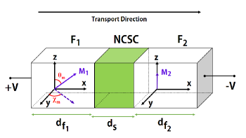
Figure 1: The schematic overview of the proposed experimental setup. In this F$|$NCSC$|$F spin valve architechture, the left F₁-layer represents a soft ferromagnet with exchange field $\bm{h}=h_{0}(\sin\theta_{m}\cos\chi_{m},\sin\theta_{m}\sin\chi_{m},\cos\theta_{m})$, where $\theta_{m}$, $\chi_{m}$ respectively represent the polar and azimuthal angle of magnetization. The right F₂-layer represents a hard ferromagnet with a fixed orientation of magnetization. The middle NCSC-layer represents a noncentrosymmetric superconductor. In this work, x-direction is assumed to be as the direction of transport.

II Theory

II.1 Model and formalism

We use the standard Bogoliubov-de Gennes (BdG) formalism to describe the behaviours of the Electron-Like-Quasi (ELQ) particle and Hole-Like-Quasi (HLQ) particle amplitudes with spin $\sigma$. The schematic overview of the proposed setup is shown in Fig.1. For our setup, the BdG equations can be written as

$$\left(\begin{array}[]{cc}\hat{\mathcal{H}}_{0}&\hat{\Delta}_{\alpha\beta}(r,r^{\prime})\\ \hat{\Delta}_{\alpha\beta}^{\dagger}(r,r^{\prime})&-\hat{\mathcal{H}}_{0}^{\dagger}\\ \end{array}\right)\left(\begin{array}[]{c}u_{n\sigma}\\ v_{n\sigma}\\ \end{array}\right)=\epsilon_{n}\left(\begin{array}[]{c}u_{n\sigma}\\ v_{n\sigma}\\ \end{array}\right)$$ (1)

where, $u_{n\sigma}$ and $v_{n\sigma}$ are the wavefunctions of ELQ particles and HLQ particles respectively. The hat sign represents a $2\times 2$ matrix, $\epsilon_{n}$ are the energy eigenvalues can be obtained by diagonalizing the BdG Hamiltonian in the respective layers. $\hat{\mathcal{H}}_{0}$ is the single particle Hamiltonian of the system, defined as

$$\hat{\mathcal{H}}_{0}=(\mathcal{H^{\prime}}+\mathcal{B})\hat{I}+\hat{\mathcal{H}}_{R}-\bm{h}\cdot\bm{\sigma}.$$ (2)

The first term in this Eq.(2) can be written as $\mathcal{H}^{\prime}=-\frac{\nabla^{2}}{2}+E_{Fi}\,+\,U_{0}\,\delta(x)$, where $-\frac{\nabla^{2}}{2}$ and $E_{Fi}$ are respectively the single particle kinetic energy and the Fermi energies in the respective layers. Here, we use standard units, viz., $\hbar=m=\mu=1$. $U_{0}\delta(x)$ is the delta like barrier potential appears at F$|$NCSC interface with $U_{0}$ as the strength of spin independent barrier potential. $\mathcal{B}$ is the in-plane external magnetic field and $\hat{\mathcal{H}}_{R}$ is the RSOC, can be defined as wu ; wu1 ; cheng1 ; acharjee1

$$\hat{\mathcal{H}}_{R}(\bm{k})=\{U_{R}\,\hat{e}_{x}\cdot(\bm{\sigma}\times\bm{k})\}$$ (3)

where, $U_{R}$ represents the strength of RSOC, $\hat{e}_{x}$ is an unit vector directed normal to the interface and $\bm{k}$ = $-i\bm{\nabla}$. The last term in Eq.(2) represents the exchange interaction, where $\bm{h}$ and $\bm{\sigma}$ are the exchange field and Pauli’s spin matrices respectively.

The gap matrix $\hat{\Delta}_{\alpha\beta}(r,r^{\prime})$ appear in the Eq.(1) is the mixture of singlet (S) and triplet (T) components for a NCSC. It has the following form linder ; acharjee1 :

$$\hat{\Delta}_{\alpha\beta}(r,r^{\prime})=\left(\begin{array}[]{cc}\Delta_{\uparrow\uparrow}(r,r^{\prime})&\Delta_{\uparrow\downarrow}(r,r^{\prime})\\ \Delta_{\downarrow\uparrow}(r,r^{\prime})&\Delta_{\downarrow\downarrow}(r,r^{\prime})\\ \end{array}\right)$$ (4)

In general, $\Delta_{\uparrow\downarrow}(r,r^{\prime})$ appearing in Eq.(4) is a superposition of the singlet (S) and the triplet (T) components that satisfies the following conditions:

$$\Delta_{\uparrow\downarrow}(r,r^{\prime}) =\Delta^{S}_{k\uparrow\downarrow}(r,r^{\prime})+\Delta^{T}_{k\uparrow\downarrow}(r,r^{\prime}),$$ (5)

$$\Delta^{T}_{k\uparrow\downarrow}(r,r^{\prime}) =\Delta^{T}_{k\downarrow\uparrow}(r,r^{\prime}),$$ (6)

$$\Delta^{S}_{k\uparrow\downarrow}(r,r^{\prime}) =-\Delta^{S}_{k\downarrow\uparrow}(r,r^{\prime}).$$ (7)

Thus in view of Eqs.(1), (2), (3) and (4) the BdG equation in an extended form can be written as

$$\left(\begin{array}[]{cccc}-h_{z}+\mathcal{H}^{\prime}+\mathcal{B}&g_{k_{-}}-h_{\text{xy}}&\Delta^{T}_{k\uparrow\uparrow}&\Delta^{S}_{k\uparrow\downarrow}+\Delta^{T}_{k\uparrow\downarrow}\\ g_{k_{+}}-h^{*}{}_{\text{xy}}&h_{z}+\mathcal{H}^{\prime}+\mathcal{B}&-\Delta^{S}_{k\uparrow\downarrow}+\Delta^{T}_{k\uparrow\downarrow}&\Delta^{T}_{k\downarrow\downarrow}\\ {\Delta^{T}_{k\uparrow\uparrow}}^{\dagger}&-{\Delta^{S}_{k\uparrow\downarrow}}^{\dagger}+{\Delta^{T}_{k\uparrow\downarrow}}^{\dagger}&h_{z}-\mathcal{H}^{\prime}-\mathcal{B}&g_{k_{+}}-h^{*}{}_{\text{xy}}\\ {\Delta^{S}_{k\uparrow\downarrow}}^{\dagger}+{\Delta^{T}_{k\uparrow\downarrow}}^{\dagger}&{\Delta^{T}_{k\downarrow\downarrow}}^{\dagger}&g_{k_{-}}-h_{\text{xy}}&-h_{z}-\mathcal{H}^{\prime}-\mathcal{B}\\ \end{array}\right)\left(\begin{array}[]{c}u_{n\uparrow}\\ u_{n\downarrow}\\ v_{n\uparrow}\\ v_{n\downarrow}\\ \end{array}\right)=\epsilon_{n}\left(\begin{array}[]{c}u_{n\uparrow}\\ u_{n\downarrow}\\ v_{n\uparrow}\\ v_{n\downarrow}\\ \end{array}\right)$$ (8)

where, $h_{xy}=h_{0}(\sin\theta_{m}\cos\chi_{m}-i\sin\theta_{m}\sin\chi_{m})$, $h_{z}=h_{0}\cos\theta_{m}$ and $g_{k\pm}=U_{R}(k_{x}\mp ik_{y})\Theta(x)$. Here $\Theta(x)$ is the Heavyside step function can be defined as

$$\Theta(x)=\left\{\begin{array}[]{rc}0,&x<0,\\ 1,&x\geq 0.\end{array}\right.$$ (9)

In order to obtain the momenta $k^{+}(k^{-})$ for the electron(holes) in the soft F-layer, we diagonalize the BdG Hamiltonian appearing in the Eq.(8). On diagonalizing, which can be found as

$$k^{\sigma}=k_{FF}\sqrt{1+Z_{0}-\sigma Z_{R}\sin\theta_{F}-\sigma X+B\pm Z_{1}}$$ (10)

where, $\sigma=\pm 1$ represent two different orientations of the spin and $k_{FF}$ represent the Fermi momentum of electron and holes at F-layer. Here, we define $Z_{0}=\frac{2U_{0}}{k_{FF}}$, $Z_{R}=2U_{R}$, $X=\frac{M_{1}}{E_{FF}}$, $B=\frac{\mathcal{B}}{E_{FF}}$ and $Z_{1}=\frac{E}{E_{FF}}$ with $M_{1}$ as the strength of magnetization of the left ferromagnetic layer, $X$ as the strength of magnetization per unit Fermi energy and $E_{FF}$ as the Fermi energy of electrons and holes in that region.

In a similar way, we represent the momenta of the ELQ(HLQ) particles in the superconducting region by $q^{+}$($q^{-}$), which are defined as

$$q^{\pm}=\sqrt{2(E_{FS}-B\pm\sqrt{E^{2}-\Delta_{\alpha\beta}^{2}})}$$ (11)

where, $E_{FS}$ is the Fermi energy of ELQ and HLQ particles in the superconducting region. Since, in the tunnelling mechanism the parallel component of momenta is conserved. So we can write,

$$k^{+}\sin\theta_{\text{F}}=k^{-}\sin\theta_{\text{A}}=q^{+}\sin{\theta_{e}}=q^{-}\sin\theta_{h}$$ (12)

where, $\theta_{F}$ and $\theta_{A}$ are respectively are the angle of incidence of the electron in F-region and the Andreev reflected angle for the hole in the superconducting region. $\theta_{e}$ is the angle of refraction for the ELQ particles, while $\theta_{h}$ is the angle of refraction for the HLQ particles.

Since, the Fermi energy in NCSC is quite different from a ferromagnet, so to characterize this, we introduce a FWM parameter $\lambda$. Physically, it is a dimensionless parameter defined as the ratio of the Fermi momentum ($q_{FS}$) in the superconducting region to Fermi momentum ($k_{FF}$) in the Ferromagnetic region, i.e. $\lambda=\frac{q_{FS}}{k_{FF}}$. The wave function $\Psi_{\text{F}}(x)$ in F-layer with any arbitrary orientation of magnetization is given by

$$\Psi_{\text{FM}}(x<0)=s_{\uparrow}[\delta_{1}\hat{e}_{1}+\delta_{2}\hat{e}_{2}]e^{ik^{+}\cos\theta_{F}x}\\ +s_{\downarrow}[-\delta_{2}^{*}\hat{e}_{1}+\delta_{1}\hat{e}_{2}]e^{ik^{-}\cos\theta_{F}x}\\ +r_{e}^{\uparrow}[\delta_{1}\hat{e}_{1}+\delta_{2}\hat{e}_{2}]e^{-ik^{+}S_{1}x}\\ +r_{e}^{\downarrow}[-\delta_{2}^{*}\hat{e}_{1}+\delta_{1}\hat{e}_{2}]e^{-ik^{+}S_{2}x}\\ +r_{h}^{\uparrow}[\delta_{1}\hat{e}_{3}+\delta_{2}\hat{e}_{4}]e^{ik^{+}S_{1}x}\\ +r_{h}^{\downarrow}[-\delta_{2}^{*}\hat{e}_{3}+\delta_{1}\hat{e}_{4}]e^{ik^{-}S_{2}x}$$ (13)

where, we define $\hat{e}_{1}=(1,0,0,0)^{T}$, $\hat{e}_{2}=(0,1,0,0)^{T}$, $\hat{e}_{3}=(0,0,1,0)^{T}$, $\hat{e}_{4}=(0,0,0,1)^{T}$, $\delta_{1}=\cos\theta_{m}$, $\delta_{2}=\sin\theta_{m}e^{-i\chi_{m}}$, $S_{1}=s_{\uparrow}\cos\theta_{\text{F}}+s_{\downarrow}\cos\theta_{\text{A}}$ and $S_{2}=s_{\uparrow}\cos\theta_{\text{A}}+s_{\downarrow}\cos\theta_{\text{F}}$. For up spin incident particle we choose $s_{\uparrow}$ = 1, $s_{\downarrow}$ = 0, while for a down spin particle $s_{\uparrow}$ = 0, $s_{\downarrow}$= 1. $\theta_{m}$ and $\chi_{m}$ are the polar angle and azimuthal angle of magnetization corresponding to the magnetization vector in the soft ferromagnetic layer. $r_{e}^{\uparrow}$ ($r_{e}^{\downarrow}$) appearing in the Eq.(13) are the normal reflection coefficients for upspin (downspin) electrons, while $r_{h}^{\uparrow}$ ($r_{h}^{\downarrow}$) are the Andreev reflection coefficients for the upspin (downspin) holes.

In a similar way, the wave function $\Psi_{\text{NCSC}}(x)$ in NCSC-layer can be written linder as

$$\Psi_{\text{NCSC}}(x\geq 0)=\frac{t_{e}{}^{\uparrow}}{\sqrt{2}}[u_{+}\Gamma_{1}+v_{+}\Gamma_{4}]e^{iq_{e}^{+}\cos\theta_{e}x}\\ +\frac{t_{e}{}^{\downarrow}}{\sqrt{2}}[u_{-}\Gamma_{2}+v_{-}\Gamma_{3}]e^{iq_{e}^{-}\cos\theta_{e}x}\\ +\frac{t_{h}{}^{\uparrow}}{\sqrt{2}}[v_{+}\Gamma_{1}+u_{+}\Gamma_{4}]e^{iq_{h}^{+}\cos\theta_{h}x}\\ +\frac{t_{h}{}^{\downarrow}}{\sqrt{2}}[v_{-}\Gamma_{2}+u_{-}\Gamma_{3}]e^{i\text{q}_{h}^{-}\cos\theta_{h}x}$$ (14)

where, $\Gamma_{1}=(\hat{e}_{1}+\hat{e}_{2}e^{-i\phi})$, $\Gamma_{2}=(\hat{e}_{1}-\hat{e}_{2}e^{-i\phi})$, $\Gamma_{3}=(\hat{e}_{4}+\hat{e}_{3}e^{-i\phi})$ and $\Gamma_{4}=(\hat{e}_{4}-\hat{e}_{3}e^{-i\phi})$. $\phi$ is the superconducting phase factor, $t_{e}^{\uparrow}$( $t_{e}^{\downarrow}$) corresponds to the transmission coefficients for up(down) spin of ELQ particles, while $t_{h}^{\uparrow}$( $t_{h}^{\downarrow}$) represents the transmission coefficients for up(down) spin of HLQ particles. The amplitudes of wavefunctions of ELQ particles and HLQ particles are given by

$$u_{\pm}(v_{\pm})=\frac{1}{\sqrt{2}}\sqrt{1+(-)\sqrt{1-\frac{|\Delta_{s}\pm\frac{\Delta_{t}}{2}|^{2}}{E^{2}}}}.$$ (15)

The reflection coefficients ($r_{e}^{\sigma}$, $r_{h}^{\sigma}$) and the transmission coefficients ($t_{e}^{\sigma}$, $t_{h}^{\sigma}$) in the wavefunctions can be determined under the following boundary conditions:

$$\Psi_{\text{FM}}(x=0^{-})=\Psi_{\text{NCSC}}(x=0^{+}),$$ (16)

$$\partial_{x}\{\Psi_{\text{NCSC}}(x=0^{+})-\Psi_{\text{FM}}(x=0^{-})\}=$$

$$2U_{int}\Psi_{\text{FM}}(x=0)$$ (17)

where, $U_{int}=U_{0}\delta(x)+\mathcal{H}_{R}$ is the interacting potential.

II.2 Calculation of Spin Conductance at the F$|$NCSC interface

To calculate the spin conductance $G_{S}(E)$, we have used the extended Blonder - Tinkham - Klapwijk (BTK) approach blonder . According to BTK formalism, the spin conductance $G_{S}^{\uparrow}(E,\theta_{F})$ for an upspin incoming electron incident at an angle $\theta_{F}$ is

$$G_{S}^{\uparrow}(E,\theta_{F})=\frac{1+X}{2}(1-|r_{e}^{\uparrow}|^{2}+|r_{e}^{\downarrow}|^{2}+|r_{h}^{\uparrow}|^{2}-|r_{h}^{\downarrow}|^{2}),$$ (18)

while for a downspin incoming electron, the the spin conductance $G_{S}^{\downarrow}(E,\theta_{F})$ is

$$G_{S}^{\downarrow}(E,\theta_{F})=\frac{1-X}{2}(1+|r_{e}^{\uparrow}|^{2}-|r_{e}^{\downarrow}|^{2}+|r_{h}^{\uparrow}|^{2}-|r_{h}^{\downarrow}|^{2}).$$ (19)

Thus, in view of this the angularly averaged spin conductance can be written as acharjee1 ; cheng1 ; blonder ; linder ; linder1

$$G_{S}(E)=G_{N}^{-1}\int_{-\frac{\pi}{2}}^{\frac{\pi}{2}}d\theta_{F}\cos\theta_{F}\{G_{S}^{\uparrow}+G_{S}^{\downarrow}\},$$ (20)

where $G_{N}$ is the tunnelling conductance for N$|$N (N for normal mattel) junction and has the following form:

$$G_{N}=\int_{-\frac{\pi}{2}}^{\frac{\pi}{2}}d\theta_{F}\frac{4\cos^{3}\theta_{F}}{4\cos^{2}\theta_{F}+Z_{0}^{2}}.$$ (21)

II.3 Spin Tunnelling Magneto-Resistance (STMR)

It is seen from Eqs.(18) and (19) that the spin conductance for spin-up particles is quite different from that of spin-down particles. Thus it generates a STMR. Moreover, it also seen from Eqs.(18) and (19) that the value STMR is depended on the magnetization strength (X). So in this work we have studied the STMR for different X and magnetic field (B). It is to be noted that STMR can be calculated by knowing the reflection and transmission coefficients from Eqs.(16) and (II.1) at the different spin subbands and then inserting them in spin conductance Eqs.(18) and (19). The STMR can be defined cheng1 as

$$\text{STMR}=\frac{G_{S}^{P}(E)-G_{S}^{AP}(E)}{G_{S}^{P}(E)}$$ (22)

where, $G_{S}^{P}(E)$ and $G_{S}^{AP}(E)$ respectively corresponds to the spin conductances at parallel and anti-parallel orientations.

II.4 Spin Current ($\bm{S}$)

Due to the non-collinear orientation of magnetization in the two ferromagnetic layers of the F$|$NCSC$|$F SV, a spin current $\bm{S}$ is generated and flows through the system even in absence of a charge current. Thus the spin current can be totally controlled by the strength and the orientation of exchange fields. Moreover, the spin currents in the ferromagnetic layers generate a torque which tends to rotate the magnetizations. The spin continuity equation can be written as

$$\partial_{t}\langle\bm{\eta}(x)\rangle+\partial_{x}\bm{S}(x)=\bm{\tau}(x)$$ (23)

where, $\partial_{t}=\frac{\partial}{\partial t}$, $\partial_{x}=\frac{\partial}{\partial x}$, $\bm{\tau}(x)=-2\langle\psi^{\dagger}(x)\big{(}\bm{\sigma}\times\bm{h}\big{)}\psi(x)\rangle$ is the Spin Transfer Torque (STT) and $\bm{\eta}(x)$ is the spin density operator related to magnetization as $\bm{m}(x)=-\mu_{B}\langle\bm{\eta}(x)\rangle$. The spin density is in general has a tensor form since it has both direction of flow in real space and a direction in spin space. However, it can be reduced to vector form by the quasi-one-dimensional nature of the geometry. The spin current can be defined as

$$\bm{S}(x)=-\frac{i}{2m}\langle\psi^{\dagger}(x)\bm{\sigma}\partial_{x}\psi(x)-\partial_{x}\psi^{\dagger}(x)\bm{\sigma}\psi(x)\rangle.$$ (24)

we can write $\bm{S}$ in terms of quasi-particle amplitudes and energies using Bogoliubov transformations:

$$\psi_{\sigma}(r)=\sum_{n}[u_{n\sigma}(r)\gamma_{n}+\eta v^{\ast}_{n\sigma}(r)\gamma^{\dagger}_{n}],$$ (25)

where $u_{n\sigma}$ and $v_{n\sigma}$ are the quasi-particle and quasi-hole amplitudes. $\gamma_{n}$ and $\gamma^{\dagger}_{n}$ are Bogoliubov quasi-particle annihilation and creation operators respectively, which satisfy the following expectation values: $\langle\gamma^{\dagger}_{n}\gamma_{m}\rangle=\delta_{mn}f_{n}$, $\langle\gamma_{m}\gamma^{\dagger}_{n}\rangle=\delta_{nm}(1-f_{n})$ and $\langle\gamma_{n}\gamma_{m}\rangle=0$. Here, $f_{n}=\big{[}\exp\big{(}\frac{\epsilon_{n}}{2T}\big{)}+1\big{]}^{-1}$ is the Fermi function which is dependent on temperature T and quasi-particle energy $\epsilon_{n}$. Calculating the reflection, transmission coefficients and inserting Bogoliubov transformations (25), the components of spin current (24) halterman5 ; moen2 ; linder5 can be represented in terms of quasi-particle amplitude as

$$S_{x}(x)=-\frac{i}{2m}\sum_{n}\Big{[}f_{n}\Big{\{}u^{\ast}_{n\uparrow}\partial_{x}u_{n\downarrow}+u^{\ast}_{n\downarrow}\partial_{x}u_{n\uparrow}\\ -u_{n\downarrow}\partial_{x}u^{\ast}_{n\uparrow}-u_{n\uparrow}\partial_{x}u^{\ast}_{n\downarrow}\Big{\}}-(1-f_{n})\Big{\{}v_{n\uparrow}\partial_{x}v^{\ast}_{n\downarrow}\\ +v_{n\downarrow}\partial_{x}v^{\ast}_{n\uparrow}-v^{\ast}_{n\uparrow}\partial_{x}v_{n\downarrow}-v^{\ast}_{n\downarrow}\partial_{x}v_{n\uparrow}\Big{\}}\Big{]},$$ (26)

$$S_{y}(x)=-\frac{1}{2m}\sum_{n}\Big{[}f_{n}\Big{\{}u^{\ast}_{n\uparrow}\partial_{x}u_{n\downarrow}-u^{\ast}_{n\downarrow}\partial_{x}u_{n\uparrow}\\ -u_{n\downarrow}\partial_{x}u^{\ast}_{n\uparrow}+u_{n\uparrow}\partial_{x}u^{\ast}_{n\downarrow}\Big{\}}-(1-f_{n})\Big{\{}v_{n\uparrow}\partial_{x}v^{\ast}_{n\downarrow}\\ -v_{n\downarrow}\partial_{x}v^{\ast}_{n\uparrow}+v^{\ast}_{n\uparrow}\partial_{x}v_{n\downarrow}-v^{\ast}_{n\downarrow}\partial_{x}v_{n\uparrow}\Big{\}}\Big{]},$$ (27)

$$S_{z}(x)=-\frac{i}{2m}\sum_{n}\Big{[}f_{n}\Big{\{}u^{\ast}_{n\uparrow}\partial_{x}u_{n\uparrow}-u_{n\uparrow}\partial_{x}u^{\ast}_{n\uparrow}\\ -u^{\ast}_{n\downarrow}\partial_{x}u^{\ast}_{n\downarrow}+u_{n\downarrow}\partial_{x}u_{n\downarrow}\Big{\}}-(1-f_{n})\Big{\{}-v_{n\uparrow}\partial_{x}v^{\ast}_{n\uparrow}\\ +v^{\ast}_{n\uparrow}\partial_{x}v_{n\uparrow}+v_{n\downarrow}\partial_{x}v^{\ast}_{n\downarrow}-v^{\ast}_{n\downarrow}\partial_{x}v_{n\downarrow}\Big{\}}\Big{]}.$$ (28)

III Results and Discussion

III.1 Spin Conductance Spectra at the F$|$NCSC interface

In this work, we study the spin transport quantities, more specifically TSC ($G_{S}$), STMR and the spin current ($\bm{S}$) for a F$|$NCSC$|$F SV. We have plotted the spin conductance $G_{S}(E)$ from the equation (20) as a function of baising energy $E$ scaled by the gap amplitude $\Delta$ of NCSC. Since NCSCs posses a mixed pairing state, so to understand the interplay of pairing symmetry on spin transport we have introduced the gap amplitude parameter $|\Delta_{\pm}|$, where $|\Delta_{\pm}|=|\Delta_{s}\pm\frac{\Delta_{t}}{2}|$. For most of our analysis we choose $\Delta_{s}=\frac{\Delta_{t}}{3}$. However to understand the impact of singlet-triplet mixing ratio on the spin conductance, we have also considered different mixing ratios too. Furthermore, to study the spin conductance spectra we set the magnetization strength, polar angle and the azimuthal angle of magnetization respectively as $X=0.9$, $\theta_{m}=0.25\pi$ and $\chi_{m}=0.5\pi$. It is to be noted here that the densities of the local charge carries in different regions of F$|$NCSC heterostructure are different. Again, the Fermi momenta for a ferromagnet is also quite different from a NCSC. So to incorporate this point we introduce a dimensionless parameter $(\lambda)$, which characterizes the FWM at the different regions. Though $\lambda$ can have any arbitrary values, however for high temperature superconductors FWM is found to be less than unity linder1 . Hence for our calculation of spin conductance acharjee1 ; linder ; linder1 , STMR and spin current, we set $\lambda=0.5$.

In most of the earlier works on tunnelling spectroscopy linder1 ; bozovic1 ; bozovic2 ; cheng ; cheng1 ; zutic1 ; zutic2 ; tanaka ; moen1 ; linder ; iniotakis ; kashiwaya ; acharjee1 , it was found that the barrier thickness play a very significant role on the transport mechanism. However, the role of barrier thickness on spin transport is yet to be understood. So, we study the variation of spin conductance with applied baising energy for different RSOC ($Z_{R}$), magnetization strength $(X)$ and in-plane magnetic field ($B$) considering initially a partially opaque barrier with $Z_{0}=1.0$ and a highly opaque barrier of barrier thickness $Z_{0}=2.0$. The result of which are presented in Figs.2 and 3 respectively. Furthermore, for a complete understanding of the quantum tunnelling mechanism and the role of barrier thickness, we have also considered a highly transparent barrier with barrier width $Z_{0}=0$ in Fig.4.

Effect of Rashba Spin Orbit Coupling (RSOC)

From the previous works, it is found that the role of RSOC in NCSC is too notable. Though RSOC has a very pivotal role in superconducting pairing, but its interplay with magnetization, magnetic field is still need to be understood. So in view of this in Fig.2 we study the effect of RSOC $(Z_{R})$ on the spin conductance $G_{S}(E)$. For all our analysis on spin conductance we consider four different choices of RSOC viz., $Z_{R}=0,0.5,1.0$ and $2.0$. Moreover, to understand the significance of external in-plane magnetic field on spin conductance we have also considered four different in-plane magnetic field strengths viz., $B=0,0.3,0.7$ and $1.0$ respectively in Figs.2(a), 2(b), 2(c) and 2(d).

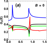
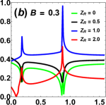
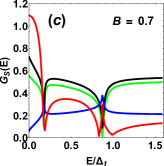
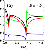
Figure 2: Spin conductance spectra for different values of $B$ and for $X=0.9$ considering $\Delta_{s}=\frac{\Delta_{t}}{3}$, $Z_{0}=1.0$, $\lambda=0.5$, $\theta_{m}=0.25\pi$ and $\chi_{m}=0.5\pi$.

It is seen that due to the formation of Andreev Bound States (ABS) nearer to the baising energies, $E=\Delta_{-}$ = $|\Delta_{s}-\frac{\Delta_{t}}{2}|$ and at $\Delta_{+}$ = $|\Delta_{s}+\frac{\Delta_{t}}{2}|$, two sharp peaks in the spin conductance are observed for $Z_{R}=1.0$ and $2.0$ in absence and for low magnetic field $B=0.3$. It is to be noted that $Z_{R}=1.0$ shows maximum conductance in both the cases. The sharpness of the peak increases nearly at $E\sim\Delta_{+}=0.83\Delta_{t}$, while it decreases at $E\sim\Delta_{-}=0.17\Delta_{t}$ for a very low value of $B=0.3$. The situation is opposite at these two points in absence of $B$. Also the sharpness is highest nealy at $E\sim\Delta_{+}=0.83\Delta_{t}$ for $B=0.3$. These results strongly indicate that in-plane magnetic field must have some significant role on the spin transport. With the further rise of $B$ to $0.7$ the sharpness of the peaks get decreased and finally for $B=1.0$ two dips are seen for all choices of $Z_{R}$ as clear from Fig.2(d). This is because in presence of strong in-plane magnetic field $B$ the exchange field becomes very strong, hence it becomes unfavourable for the superconducting pairing. Thus ABS get suppressed and is characterised by the dips in Fig.2. It is also to be noted that for Rashba free case $Z_{R}=0$ and for low RSOC value $Z_{R}=0.5$, two sharp dips are also observed for all choices of magnetic field. However, for $Z_{R}=0$, a sharp rise is seen in case of $B=1.0$. Moreover, it is also observed from Fig.2(d) that for $B=1.0$ the spin conductance becomes maximum for $Z_{R}=0.5$ and it sharply decreases as the biasing energy approaches the gap energies $\Delta_{\pm}$ for all choices of $Z_{R}$.

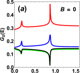
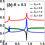
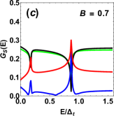
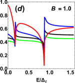
Figure 3: Spin conductance spectra for different values of $B$ and for $X=0.9$ considering $\Delta_{s}=\frac{\Delta_{t}}{3}$, $Z_{0}=2.0$, $\lambda=0.5$, $\theta_{m}=0.25\pi$ and $\chi_{m}=0.5\pi$.

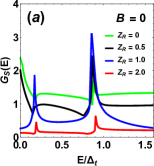
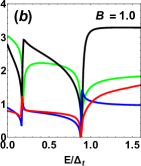
Figure 4: Spin conductance spectra for different values of $B$ and for $X=0.9$ considering $\Delta_{s}=\frac{\Delta_{t}}{3}$, $Z_{0}=0$, $\lambda=0.5$, $\theta_{m}=0.25\pi$ and $\chi_{m}=0.5\pi$.

A nearly similar characteristics are also seen in Fig.3 for a strongly opaque barrier with $Z_{0}=2.0$. However in this case, $Z_{R}=2.0$ shows maximum conductance for all values of $B$. From Figs.3(a) and 3(b) we have seen that though two sharp peaks still appears for $Z_{R}=1.0$ and $2.0$ for low values of magnetic field $B$, but the sharpness of the peak is more at $E=0.83\Delta_{t}$ than $E=0.17\Delta_{t}$ for both $B=0$ and $B=0.3$ cases. With the rise of $B$ to 0.7 conductance get decrease but sharpness of the peaks retain as seen from Fig.3(c). It indicate that for a strongly opaque barrier a moderate value $B$ is also suitable for the formation of ABS. For the magnetic field $B=1.0$, a totally different characteristics is seen. In this case for $Z_{R}=2.0$, the spin conductance is maximum for zero bias condition. However, as the bias voltage is switched on $G_{S}$ shows a gradual fall but shows two sharp dips exactly at $\Delta_{\pm}$. For $0\leq Z_{R}<1$, the spin conductance spectra is quite similar. In all these cases, $G_{S}$ initially decreases monotonically from a maxima with the rise of $E$ and then shows a sharp minima exactly at $E=\Delta_{\pm}$. It is also seen that the sharpness of the dips are too strong at $E=\Delta_{+}=0.83\Delta_{t}$ than at $E=\Delta_{-}=0.17\Delta_{t}$.

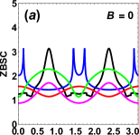
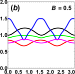
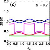
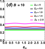
Figure 5: Variation of ZBSC with polar angle of magnetization $\theta_{m}$ for different RSOC ($Z_{R}$) and in-plane magnetic field strength ($B$). The figures are drawn for a partially transparent barrier with barrier width $Z_{0}=0.1$, considering azimuthal angle $\chi_{m}=0.5\pi$ and FWM $\lambda=0.5$.

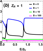
Figure 6: Spin conductance spectra for different values of $B$ considering $\Delta_{s}=\frac{\Delta_{t}}{3}$, $Z_{0}=0$, $\lambda=0.5$, $X=0.9$, $\theta_{m}=0.5\pi$ and $\chi_{m}=0.5\pi$.

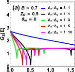
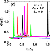
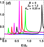
Figure 7: Spin conductance spectra for different $\Delta_{t}:\Delta_{s}$ and $\theta_{m}$ values considering $\chi_{m}=0.5\pi$, $Z_{0}=0.1$, $\lambda=0.5$ and $X=0.9$. We choose $Z_{R}=0.5$, $B=0.7$ for plots (a) and (b), while $Z_{R}=1.2$, $B=0$ for plots (c) and (d).

In case of a highly transparent barrier with barrier thickness $Z_{0}=0$, we have seen form Fig.(4) that there exist a suppression of spin conductance from maxima for region $0\leq E\leq\Delta_{-}$ in absence and for low $Z_{R}$ values. In case of higher $Z_{R}$ values i.e. $1.0$ and $2.0$, the conductance spectrum shows a gradual rise followed by a maxima at $\Delta_{-}$. For the region $\Delta_{-}\leq E\leq\Delta_{+}$, the spin conductance $G_{S}$ of the system shows a slow rise nearly at both the points $\Delta_{\pm}$ for $Z_{R}=1.0$ and $2.0$. An exactly opposite characteristics is seen for $Z_{R}=0$ and $0.5$. Though for an transparent barrier with $B=0$, Rashba free cases shows maximum conductance nearly for all biasing voltages however, at $E=\Delta_{\pm}$, $Z_{R}=1.0$ spectra shows maximum conductance as observed from Fig.4(a). As soon as the magnetic field is switched on with $B=1.0$, an exactly opposite characteristics is seen. In this case, also two sharp dips are observed for $Z_{R}=1.0$ and $2.0$ subsequently followed by two sharp peaks for biasing energy nearly equal to $\Delta_{\pm}$. It is seen from Fig.4(b) that for a transparent barrier with $Z_{R}=0$ and $0.5$, the spin conductance spectra shows maximum conductance in presence of a magnetic field $B=1.0$. Thus from Figs.2, 3 and 4 it can be conclude that the spin conductance $G_{S}$ is not only dependent on barrier thickness $Z_{0}$, but the in-plane magnetic field strength $B$ and RSOC strength $Z_{R}$ play very important role in the formation of ABS in F$|$NCSC heterostructure. It is seen that pairing and formation of ABS in NCSCs with moderate RSOC is suitable for a low magnetic field strength $B$. However, for NCSCs having moderately large RSOC and with a strongly opaque F$|$NCSC interface, moderate values of in-plane magnetic field is also found to be suitable.

It should be noted that the spin conductance is non zero even at $\theta_{m}=0$ and it has a strong correlation with orientations of magnetization ($\theta_{m}$, $\chi_{m}$), magnetization strength ($X$), the in-plane magnetic field ($B$) and RSOC ($Z_{R}$) as seen from Figs.2, 3 and 4. So, in order to understand the orientation dependence of $G_{S}$, we study the Zero Bias Spin Conductance (ZBSC) as a function of polar angle of magnetization ($\theta_{m}$) in Fig.5 for different choices of RSOC $Z_{R}$ and in-plane magnetic field strengths $B$. For all our ZBSC spectra, we set azimuthal angle $\chi_{m}=0.5\pi$, magnetization strength $X=0.7$ and FWM as $\lambda=0.5$. Moreover, we consider a partially opaque barrier with $Z_{0}=0.1$ for our analysis. Though many attempts had been made earlier to explain the ZBC in superconductors, but among them the most promising reason are due to phase mismatch of the transmitted ELQ particles and HLQ particles as reported in tanaka and the mismatch of Fermi momentum in different regions (i.e. FWM) as reported in zutic1 ; zutic2 . It is seen from Figs.5(a) and 5(b) that for all choices of $Z_{R}$, ZBSC spectra shows an oscillatory behaviour in absence and low magnetic field regime, i.e. with $B=0$ and $0.5$ respectively. A sharp Zero Bias Spin Conductance Dip (ZBSCD) is seen at $\theta_{m}=0,0.5\pi$ and $\pi$ for $Z_{R}=0,1.0$ and $2.0$ in absence of $B$, while a Zero Bias Conductance Peak (ZBSCP) is found to be observed at the same positions for $Z_{R}=1.5$ as seen from Fig.5(a). The oscillatory behaviour of the ZBSC gradually decreases with the rise of $B$ as seen from Figs.5(b), 5(c) and 5(d). It is also observed from Figs. 5(b) and 5(c) that with the increase in $B$ from $0.5$ to $0.7$, there exist a phase reversal for both low $Z_{R}=0$ and high RSOC values viz.,$1.5$ and $2.0$.

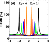
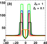
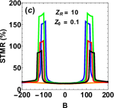
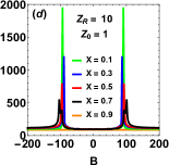
Figure 8: Variation of STMR with magnetic field (B) for different choices of $X$, $Z_{0}$ and $Z_{R}$ considering $\Delta_{s}=\frac{\Delta_{t}}{3}$ and $\lambda=0.5$.

The oscillatory behaviour of ZBSC spectra nearly die out for a very high value of $B$ to $10$ for any arbitrary value of $Z_{R}$ as seen from Fig.5(d). So, it can be concluded ZBSC that has a strong dependence on the magnetization, magnetic field and RSOC. Notwithstanding, for an experimentally feasible design of F$|$NCSC heterostructure, moderate value of $B$ and NCSCs with moderate RSOC are mostly suitable.

Effect of in-plane magnetic field $B$

It is already seen from the preceding section that the orientation of magnetization plays a significant role in the formation of ABS and pairing mechanism in NCSC. Moreover, the formation of spin current, STMR and triplet-singlet correlation in an SV are also dependent on the orientation of magnetization. Thus the significance of an in-plane magnetic field in the context of SV devices is highly inherent. So to investigate the role of in-plane magnetic field $B$ on spin conductance, we have studied the variation of $G_{S}$ with $E/\Delta_{t}$ for different choices of $B$ as shown in Fig.6. We consider a transparent barrier with $Z_{0}=0$, FWM $\lambda=0.5$, magnetization strength and orientations respectively are $X=0.9$, $\theta_{m}=0.5\pi$ and $\chi_{m}=0.5\pi$ for this study of spin conductance. It is to be noted here that the increasing value of $B$ suppresses the spin conductance of the system for any choices of RSOC. For Rashba free case with $Z_{R}=0$, there exist two sharp dips appear at $\Delta_{\pm}$ for all choices of $B$ as seen from Fig.6(a). It is quite obvious as the Rashba free materials doesn’t offer unconventional superconductivity and hence the ABS are totally suppressed. However, when the RSOC is increased to $Z_{R}=1$, two sharp peaks are observed exactly at $\Delta_{\pm}$ in absence of $B$ as seen from Fig.6(b). It indicate the formation ABS and presence of an unconventional superconductivity in the SV.

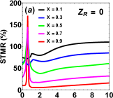
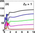
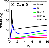
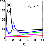
Figure 9: Variation of STMR with barrier width $Z_{0}$ for different choices of $X$, $B$ and $Z_{R}$ considering $\Delta_{s}=\frac{\Delta_{t}}{3}$, $\theta_{m}=0.25\pi$ $\chi_{m}=0.5\pi$ and $\lambda=0.5$. Figs.(a) and (b) are plotted for different choices of $X$ with $B=0.1$, while Figs.(c) and (d) are plotted for different $B$ values with $X=0.9$.

It is seen that if the magnetic field is switched on, then the pairing and the formation of ABS will get suppressed. It is because for large magnetic field potentially destroy the superconducting ordering and hence the pairing mechanism. Thus for spin conductance and fabrication of an F$|$NCSC$|$F, NCSC materials with moderate RSOC is highly suitable. Moreover, though large value of in-plane magnetic field is not suitable as seen from Fig.6, but for NCSC with large RSOC with opaque interface a low in-plane magnetic field can be preferred as already seen from Figs.2 and 3.

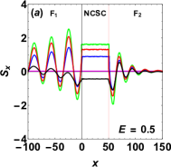
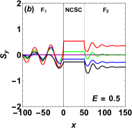
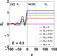
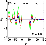
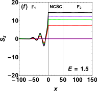
Figure 10: Spatial variation of spin current for two different bias voltages viz., $E=0.5$ and $1.5$. The components of spin current ($S_{x},S_{y},S_{z}$) are plotted in y-axes are the multiple of $10^{-4}$, while the spatial coordinate ($x$) is taken in nanometre scale. The figures are plotted for $\Delta_{s}=\frac{\Delta_{t}}{3}$, $\lambda=0.5$, $Z_{0}=0.1$, $Z_{R}=1$, $X=0.9$ and $\chi_{m}=0.5\pi$.

Effect of singlet-triplet mixing ratio $\Delta_{s}:\Delta_{t}$

It is of our interest to study the role of pairing amplitude on spin conductance. So, in Fig.7 we study the variation of spin conductance $G_{S}$ with $E/\Delta_{t}$ for different choices of singlet-triplet mixing ratios. For our analysis, we consider a partially transparent barrier with barrier thickness $Z_{0}=0.1$, FWM $\lambda=0.5$, magnetization strength $X=0.9$ and the azimuthal angle $\chi_{m}=0.5\pi$. Furthermore, we consider $B=0.7$ and $Z_{R}=0.5$ for our Figs.7(a) and 7(b). It is seen that the spin conductance has been concealed at $\Delta_{\pm}$ for $\Delta_{t}\leq\Delta_{s}$ in both the cases as already seen in Figs.2, 3, 4 and 6 too. It is to be noted that if $\Delta_{t}>\Delta_{s}$, the spin conductance falls linearly which indicate that the absence of ABS in such materials. It is also seen that though triplet correlation is favoured in many NCSCs however, the percentage of singlet correlation is always greater than the triplet correlation in NCSC. It is also observed that the sharpness of the dips increases with the change in $\theta_{m}$ from $0$ to $0.25\pi$. Beside that we also noted that for $\theta_{m}=0$ $E=\Delta_{-}$ provides maximum suppression, while for $\theta_{m}=0.25\pi$ $E=\Delta_{+}$ provides the same. Though ABS is seen in Figs.7(a) and 7(b) however as the magnetic field is switched off and RSOC is increased to $Z_{R}=1.2$, superconducting behaviour is achieved again. The singlet-triplet correlation in such cases is very significant and are strongly favourable for the formation of ABS at $\Delta_{\pm}$ as seen in Figs.7(c) and 7(d). Moreover, it is also observed that with the increase in the singlet components the ABS will approach to each other and also found to be observed at lesser bias voltages. So from the Fig.7 it can be concluded that ABS can be tuned by singlet-triplet pairing ratio, in-plane magnetic field and also by RSOC. For an experimentally suitable scenario, NCSC with greater singlet components than triplet are mostly suitable. Moreover, arbitrary orientation of magnetization is mostly suitable for fabrication purpose.

III.2 Spin Tunnelling Magneto-Resistance (STMR)

Over the last two decades, MTJs have gained attention owing to its robust physics along with the potential applications in spintronic devices. The discovery of giant Tunnelling Magneto-Resistance (TMR) binasch ; baibich ; parkin ; chappert in MgO based MTJ is one of the key reason behind its increased application in Magnetic Random Access Memory (MRAM) and magnetic sensors. The study of TMR reveals many novel properties about F-N and F-S based MTJs over the years. These studies mainly involves magnetic response of MTJ, spin alignments, dependence on temperature and barrier width. Introduction of an NCSC as a spacer can enhance the TMR value and hence found to be useful to fabricate ultra fast cryogenic MRAM. The basic reason to consider NCSC as a spacer is because of the existence of the lack of inversion symmetry and hence it shows unconventional superconductivity and possess a strong RSOC. Moreover, they can also support flow of polarized current. In view of this, we have studied the variation of STMR ($\%$) as a function of in-plane magnetic field ($B$) in Fig.8 and barrier width ($Z_{0}$) in Fig.9 for different magnetization strengths $X$, RSOC $Z_{R}$. We again set, $\Delta_{s}=\frac{\Delta_{t}}{3}$, $\lambda=0.5$ and a consider nearly transparent barrier with $Z_{0}=0.1$ in Figs.8(a), 8(b) and 8(c), while in Fig.8(d) we choose a partially opaque barrier with $Z_{0}=1$. In all the cases two sharp symmetric peaks are observed which arises due to the opposite alignment of the spins. For Rashba free case $Z_{R}=0$ with a highly transparent barrier $Z_{0}=0.1$, these peaks are observe for a significantly low magnetic field. However, it is seen that STMR value decayed too rapidly for large value of $B$ as seen from Fig.8(a). It is to be noted here that the STMR increases with the increase in $X$ and becomes maximum for $M=0.9E_{FF}$ in this case. With the rise of $Z_{R}$ to 1, the peaks dissappear and two flat region are observed for a moderately strong field as seen from Fig.8(b). It is due to the enhancement of opposite spin correlation with RSOC. A similar scenario is also observed from Fig.8(c) for $Z_{R}=10$. However, in this case the flat regions appear at a very strong magnetic field $B$. For, a partially opaque barrier ($Z_{0}=1$) with $Z_{R}=10$, the flatness disappears and two sharp peaks reappear for large values of $B$ as seen from Fig.8(d). In this case a very giant STMR value ($\sim 2000\%$) is observed for a magnetization strength of $M=0.1E_{F}$ at a magnetic field $B$ $\sim 100$. It is also seen from Fig.8(d) that the STMR $(\%)$ drastically reduced as $M\rightarrow E_{FF}$ and it becomes minimum for $M=0.9E_{FF}$. It is to be noted that the STMR value reduces to zero for $M=E_{FF}$ as seen earlier from Eqs.(18) and (19). An exactly opposite scenario is seen from Fig.8(a) for a highly transparent barrier ($Z_{0}=0.1$) with $Z_{R}=0$. In this case for $M=0.9E_{FF}$ STMR $(\%)$ is found to be maximum. Thus it can be inferred that for the fabrication of MTJs with NCSC having large RSOC, moderate magnetization strength can be found to be useful. However, a very strong magnetic field is required for this purpose. It can also be concluded that with the increase in barrier width the STMR($\%$) increases. Hence, NCSC’s with moderate or strong RSOC and F having low exchange energy with partially opaque barrier between them is highly preferable for development of an MTJ with NCSC as a spacer.

We have seen from above that the role of barrier width $Z_{0}$ is too inherent to determine the STMR value of an MTJ. Thus to understand the role of $Z_{0}$ completely we have also studied the variation of STMR ($\%$) with $Z_{0}$ in Fig.9 for different choices of $Z_{R}$, $X$ and $B$. More specifically in Figs.9(a) and 9(b), we have studied the variation of STMR ($\%$) with $Z_{0}$ for different choices of $X$ having a fixed magnetic field $B=0.1$, while in Figs.9(c) and 9(d) we have considered different $B$ values with a fixed magnetization strength $X=0.9$. It is seen that for Rashba free case with the increase in $Z_{0}$, the STMR $(\%)$ sharply increases initially for all $0.5\leq X<1.0$ and reaches a maximum at $Z_{0}\sim 0.5$. With the further rise in $Z_{0}$, the STMR value shows a sharp decrease followed by a gradual rise and saturates at large values of $Z_{0}$ in all cases of $X$ as seen from Fig.9(a). It is to be noted here that for $X=0.1$ and $0.3$, STMR value is found to be too low and no significant peaks are observed which is in accordance with the result found in Fig.8(a). A totally different characteristics has been observed from Fig.9(b) in low $Z_{0}$ regions with RSOC is increased to $Z_{R}=1$. In this case with the increase in $Z_{0}$, the STMR value initially fluctuate and gradually saturates for $Z_{0}>2$ for all choices of $X$. It is to be noted here that in both the cases, $M=0.1E_{FF}$ shows maximum STMR value for large values of $Z_{0}$ as seen from Figs.9(a) and 9(b). A similar peak is also observed nearly at the same position in Rashba free case $Z_{R}=0$ with $B=0$ and $1$, as seen from Fig.9(c). It is to be noted that for a moderate and strong field $B$, the peak gets disappeared and STMR value shows a linear rise and saturates with the increase in $Z_{0}$. The STMR spectra shows a quite similar behaviour for $Z_{R}=1$ with $B=0$ and $1$ also as seen from Fig.9(d). However, in this case STMR value gets reduced for large value of $B$. It is to be noted that there exist two sharp peaks for $Z_{0}<2$ with $B=0$, which is in accordance with our Fig.8(b). A similar pattern is also seen for $B=1$. However for this case the STMR value becomes maximum for $Z_{0}\sim 2$. Moreover, from Figs.9(a) a large STMR value of $\sim 170\%$ is seen for $X=0.9$ with $B=0.1$. It is also to be noted that this STMR value decreases to $\sim 50\%$ for $Z_{R}=1$ as seen from Figs.9(b). As soon as the magnetic field is switched off, the STMR value is found to be $\sim 150\%$ in absence of RSOC as seen from Fig.9(c). However, for $Z_{R}=1$ with $B=0$, the STMR value is slightly reduced. It is to be noted that though the STMR ($\%$) value is ($\sim 170\%$) in Rashba free case, but for $Z_{R}=1$ it decreases to ($\sim 50\%$) for $X=0.9$ seen from Fig.9(b). As it is seen that there exist two sharp peaks for $B=0$ and $1$, however for large value of $B$ the peaks disappeared again and no significant change is seen from Rashba free case.

III.3 Spin Current

To understand the role of exchange coupling and its interplay with the external bias voltages and in-plane magnetic filed applied to the proposed system, we have examined the behaviour of the spin current that exist in the SV. More specifically, we have investigated the components of spin current ($S_{x},S_{y},S_{z}$) as a function of the spatial coordinate $x$ at low bias ($E=0.5$) in top panel and high bias ($E=1.5$) in bottom panel of Fig.10. The positions of the interfaces are indicated by the vertical line with origin is chosen to be the F$|$NCSC interface. In our setup, the left F₁-layer represent a soft ferromagnet with exchange field $\bm{h}_{1}=h_{0}(\sin\theta_{m}\cos\chi_{m},\sin\theta_{m}\sin\chi_{m},\cos\theta_{m})$, while the right F₂-layer represent a hard ferromagnet with exchange field $\bm{h}_{2}=h_{0}(0,0,1)$ as already mentioned above. For our analysis we set, $\Delta_{s}=\frac{\Delta_{t}}{3}$, $\lambda=0.5$, $X=0.9$, $\chi_{m}=0.5\pi$, $Z_{0}=0.1$ and $Z_{R}=1$. Furthermore, we have also considered six different choices of the polar angle of magnetization $\theta_{m}$ ranging from $0$ to $\pi$ in each panel of Fig.10. It is observed that for parallel ($\theta_{m}=0$) and anti parallel($\theta_{m}=\pi$) orientations of the magnetizations the spin current vanishes, which is quite obvious because of the vanishing STT. It is also seen that if the polar angle $\theta_{m}$ of exchange field is slightly rotated to an angle $0.1\pi$, a negative spin current flows in the F₁ and NCSC region. With the further rotation of $\theta_{m}$ the spin current reverses its polarization and becomes maximum for the orthogonal configuration as seen from the Fig.10(a). A similar behaviour is also observed earlier in Refmoen2 ; halterman5 ; halterman6 ; linder5 . If $\theta_{m}$ is rotated further to $0.7\pi$ the spin current decreases. Since the spin current is conserved in the NCSC region all the components of $\bm{S}$ remains constant. In the hard ferromagnet since the exchange field is along the z-direction, it is observed that the transverse components $S_{x}$ and $S_{y}$ decayed too rapidly, while the longitudinal component $S_{z}$ remains constant as seen from Fig.10. It is to be noted here that with the increase in bias voltage $E$ to $1.5$ the $S_{y}$ and $S_{z}$ spin current increases, however $S_{x}$ nearly remains same as seen from Figs.10(a) and 10(d). It is because $S_{x}$ is primarily driven by the spin torque which exists. It is to be noted that the $S_{y}$ component of spin current is opposite in phase with $S_{x}$ and $S_{z}$ in both biasing situation. For low biasing it becomes negative for angle $\theta_{m}\leq 0.3\pi$ and decayed for orthogonal orientation. However, for a high biasing $S_{y}$ component becomes positive for all orientations as seen from Figs.10(b) and 10(e). It is also observed that the $S_{z}$ component of the spin current increases very rapidly in the F₁ region for high biasing as seen from Figs.10(c) and 10(f).

IV Conclusions

In summary, in this paper we have investigated the spin transport in the F$|$NCSC$|$F SV. More specifically, the TSC, STMR and the spin current have been studied for an experimentally suitable parameter set of the proposed SV. To study the normalized TSC at the F$|$NCSC interface we use an extended BTK approach and the scattering matrix formalism. We consider a Rashba type spin orbit coupling (RSOC), different strength, alignments of the exchange field and also for different singlet triplet mixing ratios of the gap amplitudes to study spin conductance. Furthermore, we consider an in-plane external magnetic field to develop the BdG Hamiltonain. We also consider a experimentally suitable value of the FWM for our investigation of spin conductance, STMR and spin current. We have also studied the STMR and spin current for different orientation of exchange field. Our results reveals many useful information of the F$|$NCSC$|$F SV system. It is seen that the spin conductance has a strong dependence on RSOC, barrier width, singlet-triplet correlation, in-plane magnetic field and magnetization. For a SV with nearly transparent barrier, NCSCs with moderate RSOC show large conductance in absence of magnetic field. It is seen that with the rise of magnetic field the spin conductance and the formation of of ABS gets suppressed. However, for partially and strongly opaque barriers, a very low and moderate value of magnetic field is suitable for formation of ABS. Beside that it can also be concluded that ABS can be tuned by singlet-triplet pairing ratio, in-plane magnetic field and also by RSOC. For fabrication of superconducting spintronic device, NCSC materials with more singlet components than triplet are mostly found to be suitable. There exist a ZBSCP and a ZBSCD which strongly indicate that spin conductance is orientation dependent. In addition, we have seen a significantly large STMR ($\%$) for the proposed setup. It is found that for fabrication of superconducting MTJs with opaque barrier, NCSC with large RSOC and high magnetization strength is highly suitable. But for a nearly transparent and partially opaque barrier, NCSCs with moderate RSOC, low magnetic field and low values of magnetization strength is strongly preferred. Moreover, from the study of spin current we have seen that it is strongly orientation dependent. With the increase in bias voltage spin current increases in traverse direction but the component along the direction of flow is almost independent.

We sincerely hope that the results of our work on F$|$NCSC$|$S SV will shed some light in the field of superconducting spintronics which can be utilized to fabricate practical devices in near future.

References

- (1) M. Johnson, Phy. Rev. Lett. 70, 2142 (1993).
- (2) F. J. Jedema, A. T. Filip and B.J.van Wees, Nature (London), 410, 345 (2001).
- (3) S. A. Wolf, et al., Science 294, 1488 (2001)
- (4) F. Casanova, et al., Phy. Rev. B. 79, 184415 (2009)
- (5) S. B. Chung, et al., Phy. Rev. Lett. 121, 167001 (2018)
- (6) M. N. Baibich, J. M. Broto, A. Fert, F. Nguyen Van Dau, and F. Petroff, Phys. Rev. Lett. 61, 2472 (1988)
- (7) G. Binasch, P. Grünberg, F. Saurenbach, and W. Zinn, Phys. Rev. B 39, 4828(R) (1989)
- (8) S. S. P. Parkin, Phys. Rev. Lett. 71, 1641 (1993)
- (9) C. Chappert et. al, Nature Mat., 6, 147 (2007).
- (10) A. Kadigrobov, R. I. Shekhter and M. Jonson, Europhys. Lett. 54, 394 (2001)
- (11) I. Z̆utić, J. Fabian and S. Das. Sarma, Rev. Mod. Phys. 76, 323 (2004).
- (12) A.I. Buzdin, Rev. Mod. Phys. 77, 935 (2005).
- (13) V. T. Petrashov, I. A. Sosnin, I. Cox, A. Parsons, and C. Troadec, Phys. Rev. Lett. 83, 3281 (1999)
- (14) M. G. Flokstra, et al., Nature (London) 12, 57 (2016)
- (15) J. C. Slonczewski, J. Magn. Magn. Mater, 159, L1 (1996)
- (16) L. Berger, Phys. Rev. B. 54, 9353 (1996)
- (17) K. Halterman, P. H. Barsic, and O. T. Valls, Phys. Rev. Lett. 99, 127002 (2007)
- (18) K. Halterman, O. T. Valls and P. H. Barsic, Phys. Rev. B 77, 174511 (2008)
- (19) A. A. Golubov and M. Yu. Kupriyanov, Nature Materials 16, 156 (2017)
- (20) Y. Zhu, A. Pal, M. G. Blamire and Z. H. Barber, Nature Materials 16, 195 (2017)
- (21) F. S. Bergeret, A. F. Volkov and K. B. Efetov, Rev. Mod. Phys. 77, 1321 (2005).
- (22) M. G. Blamire and J. W. A. Robinson, J. Phys. Cond. Matter, 26, 453201, (2014)
- (23) M. Eschrig, Phys. Today, 64(1), 43 (2011)
- (24) M. Eschrig, Rep. Prog. Phys. 78(1), 104501(2015)
- (25) J. Bardeen, L. N. Cooper and J. R. Schrieffer, Phys. Rev. 108, 1175 (1957).
- (26) S.S. Saxena, et al., Nature (London) 406, 587 (2005)
- (27) D. Aoki, et al., Nature (London) 413, 613 (2001).
- (28) C. Pfleiderer et al., Nature (London) 412, 58 (2001).
- (29) N.T. Huy, et al., Phys. Rev. Lett. 99, 067006 (2007).
- (30) E. Bauer, et al., Phys. Rev. Lett. 92, 027003 (2004).
- (31) E. Bauer, I. Bonalde, and M. Sigrist., Low Temp. Phys. 31, 748 (2005).
- (32) E. Bauer, et al., J. Phys.Soc. Jpn. 76, 051009 (2007).
- (33) G. Motoyama, et al., J. Phys. Conf. Ser. 400, 022079 (2012).
- (34) I. Kawasaki, et al., J. Phys. Soc. Jpn 82, 084713 (2013).
- (35) T. Akazawa, et al., J. Phys. Cond. Matter 16, L29 (2009).
- (36) V. K. Anand, et al., Phys. Rev. B. 83, 064522 (2011).
- (37) M. Smidman, et al., Phys. Rev. B. 89, 094509 (2014).
- (38) V. K. Anand, et al., Phys. Rev. B. 90, 041513 (2014).
- (39) B. T. Matthias, V. B. Compton and E. Corenzwit, J. Phys. Chem. Solids 19, 130 (1961).
- (40) R. P. Singh, et al., Phys. Rev. Lett. 112, 107002 (2014).
- (41) V. K. Pecharsky, L. L. Miller and K. A. Gschneidner, Phys. Rev. B 58, 497 (1998).
- (42) A. D. Hillier, J. Quintanilla and R. Cywinski, Phys. Rev. Lett. 102, 117007 (2009).
- (43) I. Bonalde, et al., New J. Phys. 13, 123022 (2011).
- (44) M. Yogi, et al., Phys. Rev. Lett. 93, 027003 (2004).
- (45) M. N. Ali, et al., Phys. Rev. B 89, 020505(R) (2014).
- (46) C. Q. Xu, et al., Phys. Rev. B 96, 064528 (2017).
- (47) J. Flouquet and A. Buzdin, Phys. World 15, 41 (2002).
- (48) S. Nandi et al., Phys. Rev. B 89, 014512 (2014).
- (49) K. V. Samokhin, E. S. Zijlstra and S. K. Bose, Phys. Rev. B. 69, 094514 (2004).
- (50) I. A. Sergienko and S. H. Curnoe, Phys. Rev. B. 70, 214510 (2004).
- (51) P. A. Frigeri, et al., Phys. Rev. Lett. 92, 097001 (2004).
- (52) S. Fujimoto, Phys. Rev. B 72, 024515 (2005).
- (53) S. Fujimoto, J. Phys. Soc. Jpn. 76, 051008 (2007).
- (54) K. Togano, et al., Phys. Rev. Lett. 93, 247004 (2004).
- (55) H. Q. Yuan, et al., Phys. Rev. Lett. 97, 017006 (2006).
- (56) P. Badica, T. Kondo, and K. Togano, J. Phys. Soc. Jpn. 74, 1014 (2005).
- (57) Y. A. Bychkov and E. I. Rashba, J. Phys. C 17, 6039 (1984)
- (58) W. Molenkamp, G. Schimdt and G. E. W. Bruer, Phys. Rev. B 64, 121202(R) (2001).
- (59) L. P. Gor’kov, E. I. Rashba, Phys. Rev. Lett. 87, 037004 (2001).
- (60) E. Bauer, et al., Phys. Rev. B 80, 064504 (2009).
- (61) K. Wakui, et al., J. Phys. Soc. Jpn. 78, 034710 (2009).
- (62) R. L. Ribeiro, et al., J. Phys. Soc. Jpn. 78, 115002 (2009).
- (63) P. K. Biswas, et al., Phys. Rev. B 84, 184529 (2011).
- (64) S. Kuroiwa, et al., Phys. Rev. Lett. 100, 097002 (2008).
- (65) J. Chen, et. al, Phys. Rev. B 83, 144529 (2011).
- (66) J. Chen, et al., New J. Phys. 15, 053005 (2013).
- (67) S. Wu, K.V. Samokhin, Phys. Rev. B 82, 184501 (2010).
- (68) C. T. Wu, O. T. Valls and K. Halterman, Phys. Rev. B. 90, 054523 (2014)
- (69) F. Romeo. et al., Sci. Rep. 5, 17544 (2015)
- (70) I. Shigeta, et al., Appl. Phys. Lett. 112, 072402 (2018)
- (71) R. Beiranvand, H. Hamzehpour, and M. Alidoust, Phys. Rev. B 94, 125415 (2016)
- (72) R. Beiranvand, H. Hamzehpour, and M. Alidoust, Phys. Rev. B 96, 161403(R) (2017)
- (73) K. Halterman, O. T. Valls and M. Alidoust, Phys. Rev. Lett. 111, 046602 (2013)
- (74) S. Wu, K.V. Samokhin, Phys. Rev. B 81, 214506 (2010).
- (75) T. Hashimoto, A. A. Golubov, Y. Tanaka, and J. Linder, Phys. Rev. B 96, 134508 (2017)
- (76) Ya. V. Fominov, N. M. Chtchelkatchev, and A. A. Golubov, Phys. Rev. B 66, 014507 (2002)
- (77) Ya. V. Fominov, A. A. Golubov, and M. Yu. Kupriyanov, JETP Lett. 77, 510 (2003)
- (78) Ya. V. Fominov, et al., JETP Lett. 91, 308 (2010)
- (79) F. Romeo and R. Citro, Phys. Rev. Lett., 111, 226801 (2013)
- (80) L. A. B. Olde Olthof, et al., Phys. Rev. B 98, 014508 (2018).
- (81) L. R. Tagirov, Phys. Rev. Lett. 83, 2058 (1999)
- (82) J. Zhu and I. N. Krivorotov, Phys. Rev. Lett. 105 207002 (2010)
- (83) M. Alidoust, K. Halterman and O. T. Valls, Phys. Rev. B 92, 014508 (2015)
- (84) M. Alidoust, K. Halterman, Phys. Rev. B 97, 064517 (2018)
- (85) K. Halterman, and M. Alidoust, Phys. Rev. B 94, 064503 (2016)
- (86) S. Acharjee and U. D. Goswami, J. Appl. Phys. 120, 263902 (2016).
- (87) J. Y. Gu, et al., Phys. Rev. Lett. 89, 267001 (2002)
- (88) G. Nowak, et al., Phys. Rev. B 78, 134520 (2008)
- (89) P. V. Leksin, et al., Phys. Rev. Lett. 109, 057005 (2012)
- (90) V. I. Zdravkov, et al., Phys. Rev. B 87, 144507 (2013)
- (91) A. A. Jara, et al., Phys. Rev. B 89,184502 (2014)
- (92) Yu. N. Khaydukov, et al., Phys. Rev. B 90, 035130 (2014)
- (93) Yu. N. Khaydukov, et al., Phys. Rev. B 97, 144511 (2018)
- (94) A. Srivastava, et al., Phys. Rev. Appl. 8, 044008 (2017)
- (95) R. S. Keizer, et al., Nature Lett. (London) 439, 825 (2006)
- (96) L. Kuerten, et al., Phys. Rev. B 96, 014513 (2017)
- (97) J. Linder and A. Sudbø, Phys. Rev. B 75, 134509 (2007).
- (98) M. Boz̆ović and Z. Radović, Phys. Rev. B. 66, 134524 (2002).
- (99) M. Boz̆ović and Z. Radović, New J. Phys. 9, 264 (2007).
- (100) I. Z̆utić and O. T. Valls, Phys. Rev. B 60, 6320 (1999).
- (101) I. Z̆utić and O. T. Valls, Phys. Rev. B 61, 1555 (2000).
- (102) Q. Cheng, D. Yu and B. Jin, Phys Lett. A 378, 2900 (2014).
- (103) Q. Cheng, B. Jin, Physica B 426, 40-44 (2013).
- (104) Y. Tanaka and S. Kashiwaya, Phys. Rev. Lett. 74, 3541 (1995).
- (105) E. Moen and O. T. Valls, Phys. Rev. B 98, 104512 (2018).
- (106) J. Linder and A. Sudbø, Phys. Rev. B 76, 054511 (2007).
- (107) S. Acharjee and U. D. Goswami, 2019 Supercond. Sci. Technol. https://doi.org/10.1088/1361-6668/ab17ec
- (108) C. Iniotakis, et al., Phys. Rev. B 76, 012501 (2007).
- (109) S. Kashiwaya, Y. Tanaka, N. Yoshida, and M. R. Beasley, Phys. Rev. B 60, 3572 (1999).
- (110) Z. An, F. Q. Liu, Y. Lin and C. Liu, Sci. Rep., 2, 388 (2012)
- (111) Q. F. Sun and X. C, Xie, Phys. Rev. B 72, 245305 (2005).
- (112) E. Moen and O. T. Valls, Phys. Rev. B 97, 174506 (2018).
- (113) J. Linder and T. Yokoyama and A. Sudbø, Phys. Rev. B 79, 224504 (2009).
- (114) K. Halterman, M. Alidoust, Phys. Rev. B 94, 064503 (2016).
- (115) K. Halterman, M. Alidoust, Supercond. Sci. Technol. 29, 055007 (2016).
- (116) J. Kopu, M. Eschrig, J. C. Cuevas, and M. Fogelström, Phys. Rev. B 69, 094501 (2004).
- (117) A. V. Samokhvalov, R. I. Shekhter and A. I. Buzdin, Sci. Rep., 4, 5671 (2014).
- (118) G. E. Blonder, M. Tinkham, T.M. Klapwijk, Phys. Rev. B 25, 4515 (1982).