Blue-noise sampling for human retinal cone spatial distribution modeling

Abstract

This paper proposes a novel method for modeling human retinal cone distribution. It is based on Blue-noise sampling algorithms that share interesting properties with the sampling performed by the mosaic formed by cone photoreceptors in the retina. Here we present the method together with a series of examples of various real retinal patches. The same samples have also been created with alternative algorithms and compared with plots of the center of the inner segments of cone photoreceptors from imaged retinas. Results are evaluated with different distance measure used in the field, like nearest-neighbor analysis and pair correlation function. The proposed method can describe features of a human retinal cone distribution with a certain degree of similarity to the available data and can be efficiently used for modeling local patches of retina.

1 Introduction

Sampling is the reduction of a continuous signal into a discrete one, or the selection of a subset from a discrete set of signals. For sampling to be effective, samples should be uniformly distributed in a way that there are no discontinuities; but at the same time, regular repeating patterns should be avoided, to prevent aliasing. In the human retina, the mosaic of the cone photoreceptor cells samples the retinal optical projection of the scene, achieving the first neural coding of the spectral information from the light that enters the eye. To solve the sampling problem, the human retina has adopted an arrangement of photoreceptors that is neither perfectly regular nor perfectly random. Local analysis of foveal mosaics shows that cones are arranged in hexagonal or triangular clusters, but extending this analysis to larger areas shows characteristics such as parallel curving and circular rows of cones associated with rotated local clusters.

There are different theories regarding the regularity and development of the cone cells mosaic. Wassle and Riemann wassle1978mosaic proposed two models based on mechanisms that assume the self-regulation of an original random pattern, one with a repulsive force acting between nerve cells and the other based on competition for territory for each neighboring cell. Later, Yellott yellott1983spectral discovered that the photoreceptors in the human retina, especially the cones, are distributed conforming to a Poisson disk distribution. He performed spectral analysis to an array of cones treated as sampling points and observed that the spectral properties of cones mosaic are representative of a Poisson disk array, with the additional restriction of a minimum distance between the center of the cells and their nearest neighbors, because of the size of the cells. This was confirmed by Galli-Resta et al., which investigated the spatial features of the ground squirrel retinal mosaics, suggesting that a minimal-spacing rule $d_{\min}$ in conjunction with an adequate density of receptors can adequately describe the array of rods and S cones galli1999modelling . Poisson disk distribution is now regarded as one of the best sampling patterns, by virtue of its blue-noise power spectrum lagae2009wang .

It is still unclear how the spatial distribution and mean density of cones can affect the sampling of a retinal image dees2011variability . An interesting evidence of this open issue is the experiment from Hofer hofer2005different which tested the perception of stimuli of small spatial scale. Showing brief, monochromatic flashes of light of half the diameter of a cone size on previously characterized retinal areas of the subjects, they described the same stimuli with a large number of hue categories, including white, blue and purple, indicating that the stimulation of two different cones with the same photopigment results in different color sensations, even with no stimuli in different regions of the retina or on other wavelength-sensitive cones.

In this study, we examined the Nearest Neigbour (NN) regularity index of the population of cones in images of real human retina. We then compared the results to another measure of spatial patterning, the Pair Correlation Function. The goal of this paper is to show that the sampling properties of the cone photoreceptor mosaic can be modeled by a blue-noise algorithm, and that they can be used to generate sampling arrays with the same features of the retinal cone mosaics. More specifically, we want to identify an algorithm capable of generating sampling arrays with the same range of densities in the retina, and use specific metrics to compare the spatial and spectral properties of the cones distribution.

2 Related Works

2.1 Retinal and Cone sampling modeling

The most recent works on retinal modeling are focused on the neural behavior wohrer2009virtual ; morillas2015towards ; morillas2017conductance ; for example, Virtual Retina by Wohrer and Kornprobst is a large scale simulation software that transforms a video input into spike trains, designed with a focus on nonlinearities, implementing a contrast gain control mechanism.

However, there have not been many attempts at modeling the cone sampling array. The first known sampling model for positioning cones in the retina with the same qualities as the human sampling was described by Ahumada ahumada1987cone . It works by placing cones, which are surrounded by circular disks representing their region of influence, starting from the center of the retina, and then applying a random jitter to each point. There is an attempt to generate a space-varying parameter model, to extend the modeling capabilities past the foveola, by varying with the eccentricity the mean radius of the cone disk, the standard deviation of the cone disk radius, and the standard deviation of postpacking jitter; but ultimately those parameters seem to be only fit for the foveola.

After their studies on human photoreceptor topography, Curcio and Sloan continued in Ahumada’s direction proposing a model of cones distribution based on regular arrays subjected to a spatial compression and a jitter, to fit the actual cones mosaic curcio1992packing . Their analysis was based on the distribution of distance and angles of neighboring cones, comparing real mosaics with artificially generated ones, and evidencing anisotropies in retinal cell spacing.

Another attempt at modeling the sampling properties of the cone mosaic was proposed by Wang wang2001modeling , which created a polar arranged array of cones and jittered the points according to the standard deviation of a Gaussian distribution, constrained by a minimal spacing rule. The comparison of power spectrum of the human foveal cones and the generated sampling arrays show similarities, and the generated arrays exhibit some basic features of the mosaic of foveal cones.

In Deering’s deering2005human human eye model, cones are modeled individually as a center points surrounded by points that define a polygon constituting the boundaries of the cell, each photoreceptor is then subjected to attractive and repulsing forces to adjust its position. This retinal synthesizer is then validated by calculating the neighbor fraction ratio and by empirically measuring the cone density in cells/mm² and comparing it from data from Curcio et al. curcio1990human .

2.2 Blue Noise Distributions

Coined by Ulichney Ulichney:87:halftoning , the term blue noise refers to an even, isotropic, yet unstructured distribution of points. Blue noise was first recognized as crucial in dithering of images since it captures the intensity of an image through its local point density, without introducing artificial structures of its own. It rapidly became prevalent in various scientific fields, especially in computer graphics, where its isotropic properties lead to high-quality sampling of multidimensional signals, and its absence of structure prevents aliasing. It has even been argued that its visual efficacy (used to some extent in stippling and pointillism) is linked to the presence of a blue-noise arrangement of photoreceptors in the retina discovered by Yellott yellott1983spectral . Over the years, a variety of research efforts targeting both the characteristics and the generation of blue noise distributions have been conducted in computer graphics.

Arguably the oldest approach to algorithmically generate point distributions with a good balance between density control and spatial irregularity is through error diffusion Floyd:1976:AAA ; Ulichney:87:halftoning , which is particularly well adapted to low-level hardware implementation in printers. Concurrently, a keen interest in uniform, regularity-free distributions appeared in computer rendering in the context of anti-aliasing Crow:1977 . Cook Cook:1986 proposed the first dart-throwing algorithm to create Poisson disk distributions, for which no two points are closer together than a certain threshold. Considerable efforts followed to modify and improve this original algorithm Mitchell:1987:GAI ; McCool:1992:HPD ; Jones05 ; Bridson:2007:FPD ; Gamito:2009:AMP . Today’s best Poisson disk algorithms are very efficient and versatile Dunbar:2006:ASD ; Ebeida:2011:EMP , even running on GPUs Wei:2008:PPD ; Bowers:2010:PPD ; Xiang:2011 .

Thanks to the pioneering work by Dippé and Wold Dippe:1985:ATS , Mitchell Mitchell:1991:SOS , Cook Cook:1986 , Shirley Shirley:1991:DAA , the computer graphics community became sensitive to the fact that noise and aliasing are tightly coupled to sampling. A large variety of optimization-based approaches has been proposed since then. Two main optimization-based approaches have been developed and presented in numerous papers: (1) on-line optimization McCool:1992:HPD ; Dunbar2006 ; Lagae:2008:ACO ; Balzer2009 ; Bowers:2010:PPD ; Ebeida2012 ; Chen2012 ; SchmaltzGBW10 ; Schlomer:2011:FPO ; Fattal2011 ; Goes2012 ; Zhou:2012:PSGNS ; Oztireli2012 ; Heck2013 ; Reinert:2016:CGF12725 , and (2) off-line optimization Ostromoukhov:2004:FHI ; Kopf:2006:RWT ; Ostromoukhov:2007:SWP ; Wachtel:2014:FTBASUSFS ; Ahmed2016:ldbn ; Ahmed2017AdaptivePointSampler , where the near-optimal solution is prepared in form of lookup tables, used in runtime. The present work uses as reference the approach called Blue Noise Through Optimal Transport (BNOT), developed by de Goes et al. Goes2012 , because it allows to achieve the best Blue Noise distribution known today.

In an effort to allow fast blue noise generation, the idea of using patterns computed offline was raised in Dippe:1985:ATS . To remove potential aliasing artifacts due to repeated patterns, Cohen et al. Cohen:2003:WTI recommended the use of non-periodic Wang tiles, which subsequently led to improved hierarchical sampling Kopf:2006:RWT and a series of other tile-based alternatives Ostromoukhov:2004:FHI ; Lagae:2006 ; Ostromoukhov:2007:SWP ; ahmed2015aa . Wachtel et al. Wachtel:2014:FTBASUSFS propose a tile-based method that incorporates spectral control over sample distributions. More recently, Ahmed et al. Ahmed2017AdaptivePointSampler proposed a 2-D square tile-based sampling method with one sample per tile and controllable Fourier spectra. However, all precalculated structures used in this family of approaches rely on the offline generation of high-quality blue noise.

3 Methods

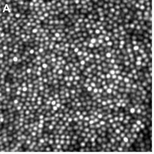
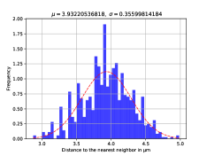
(a) 1-A

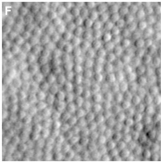
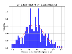
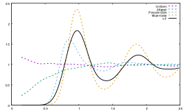
(b) 1-F

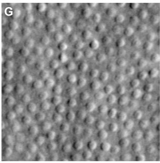
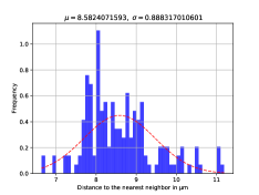
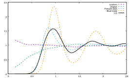
(c) 1-G

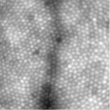
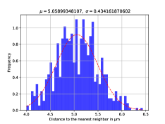
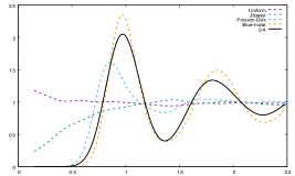
(d) 2-A

Figure 2: From left to right: The picture of the patch of retina, the point samples extracted from the cones’ location, Nearest neighbor analysis with mean and standard deviation, Pair Correlation Function. a-d. Images from Scoles et al. scoles2014vivo e. Image from Roorda & Williams roorda1999arrangement .

The cone mosaics used for this work are from previously published images of patches of real human retinas, as shown in the leftmost boxes of Figures 2 through 5; they were acquired from the pdf versions of the papers or html, if available, and saved as png images. The pictures are from different subjects of various ages and were obtained with different techniques, from histological tissue prepared for electronic microscopic imaging in curcio1990human ; jonas1992count ; curcio1991distribution ; gao1992aging , to the most recent in vivo imaging techniques, using adaptive optics like deformable mirrors coupled with a wavefront sensor to compensate for the ocular aberrations of the eye roorda1999arrangement ; song2011variation ; scoles2014vivo ; wong2015vivo . The x and y coordinates of the cells inner segments were manually plotted using WebPlotDigitizer rohatgi2011webplotdigitizer . This preliminary work has been based on a relatively small dataset sue to the difficulty of finding wide collections of retinal images. We understand these difficulties related also with problem of the use of different imaging techniques and tissue preparation and we hope to have larger datasets in the future. When analyzing the points distribution, the distance between the cone centers was converted in real $\upmu$m on the retina by multiplying them with the appropriate scale factor of the image, determined by the size of the sample window’s side. Conversion from degrees was performed according to the model from drasdo1974non , with one degree of visual angle equal to 288 $\upmu$m on the retina. Cone spacing values are compatible with Wyszecki and Styles wyszecki1982color , with the exception of the data from gao1992aging exhibiting lower values, probably due to post mortem shrinkage. Retinas 6, 7-A and 7-B have been cropped during analysis because they didn’t fully fill the sampling window, and would have included uncharacterized areas.

3.1 Analysis of point process

In this section, we briefly introduce basic notions from Stochastic Point Processes Illian2008 . A point process $\mathcal{S}$ is a stochastic generating point in a given domain $\Omega$ (here, $[0,1)^{s}$). We denote by $P_{n}:=\{\mathbf{x}^{(1)},\mathbf{x}^{(2)},\cdots,\mathbf{x}^{(n)}\}\subset\Omega$ a realization of a point process with $n$ samples. A point process $\mathcal{S}$ is stationary if it is invariant by translation, and isotropic if it is invariant by rotation. More formally, if we assume $\mathbf{P}$ a probability measure, $\mathcal{S}$ is stationary if $\forall\mathbf{x}\in\mathbb{R}^{s}$

$$\mathbf{P}(\mathcal{S}(\Omega))=\mathbf{P}(\mathcal{S}(\Omega-\mathbf{x}))\,,$$ (1)

and isotropic if any rotation or translation of $\mathcal{S}$ have the same statistical properties. We also define the density of a point set as the average number of samples inside a region $B$ of volume $V_{B}$ around a sample $\mathbf{x}$.

$$\lambda(x):=\frac{B(x)}{V_{B}}\,.$$ (2)

This density is constant for isotropic and stationary point processes. A sampler generating sets with a non constant density is sometimes called a non-uniform sampler. To characterize isotropic stationary point processes, the Pair Correlation Function (PCF) is a widely used tool. Such function is a characterization of the distribution of pair distances of a point process. Oztireli Oztireli2012 devised a simplified estimator for this measure in the particular case of isotropic and stationary point processes. The PCF of a pointset $P_{n}$ in the unit domain $[0,1)^{s}$ is given by

$$\varrho(r)=\frac{1}{n^{2}r^{s-1}}\sum_{i\neq j}k_{\sigma}(r-d(\mathbf{x}^{(i)},\mathbf{x}^{(j)})),$$ (3)

where $d(\mathbf{x}^{(i)},\mathbf{x}^{(j)})$ is a distance measure between $\mathbf{x}^{(i)}$ and $\mathbf{x}^{(j)}$. The factor $k_{\sigma}$ is used to smooth out the function. Oztireli relies on this smoothing to assume ergodicity for all sets. He uses the Gaussian function as a smoothing kernel, but one could use a box kernel or a triangle kernel instead. To compute a PCF, we use this estimator with 3 parameters, the minimal $r$, $r_{\min}$, the maximal $r$, $r_{\max}$ and the smoothing value $\sigma$. Those values are usually chosen empirically. Note that as the number of samples increase, the distances between samples will be very different for similar distributions. To alleviate this, we normalize the distances in our estimations using the maximal possible radius for $n$ samples (gamito2009 , Eq (5)).

In Figure 1, we illustrate how the PCF of several point processes captures the spectral content of the point distribution: a pure uniform sampling, Greean-Noise and Pink-Noise samplers obtained using ahmed2015aa , a jittered sampler (for $N$ samples, subdivision of the domain into regular $\sqrt{N}\times\sqrt{N}$ square tile and a uniform random sample is drawn in each tile), a Poisson-Disk sampler Bridson:2007:FPD and a Blue-noise sampler (BNOT) Goes2012 .

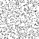
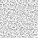
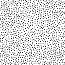
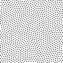
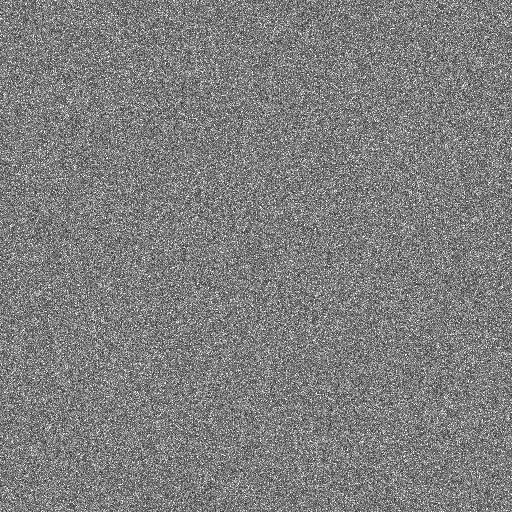
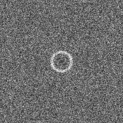
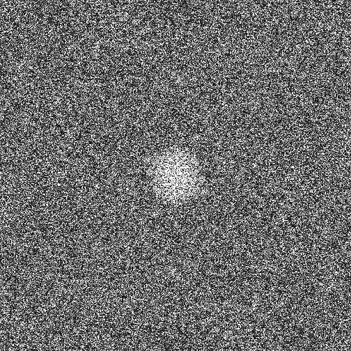
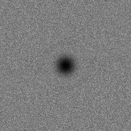
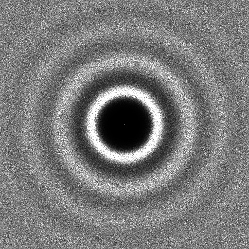
Figure 1: PCF of various 2-D samplers. Fist row from left to right: Realizations of 1024 samples from a uniform $(a)$, a Green-Noise sampler $(b)$, a Pink-Noise sampler $(c)$, a jittered $(d)$, a Poisson-disk $(e)$ and a Blue-Noise sampler $(f)$. The second row shows the Fourier specrtum (power spectrum) of each sampler ($(g)-(l)$, spectrum computed on 4096 samples). The PCFs capture the spectral content of each sampler as shown in $(m)$.

4 Results and discussion

Regularity index, or conformity ratio is a quantitative method used for assessing spatial regularity of photoreceptor distributions wassle1978mosaic ; eglen2012cellular ; cook1996spatial . A k-d tree structure has been used to find the nearest neighbor for each point, the euclidean distance was calculated for each pair found this way and all the results are classified in histograms. Each distribution of nearest neighbours can be described by a normal Gaussian distribution described by the equation

$$P(x)=\frac{1}{{\sigma\sqrt{2\pi}}}e^{{{-\left({x-\mu}\right)^{2}}\mathord{\left/{\vphantom{{-\left({x-\mu}\right)^{2}}{2\sigma^{2}}}}\right.\kern-1.2pt}{2\sigma^{2}}}}\,.$$ (4)

where $\mu$ is the mean of the distribution and $\sigma$ the standard deviation of the measurements. The regularity index is expressed by the ratio of the mean $\mu$ by the standard deviation $\sigma$. This index is reported to be 1.9 for a full random sampling and the more regular the arrangement, the higher the value, usually 3-8 for retinal mosaics.

Regularity indexes for retinal data are shown in Table 1. In contrast with previous claims, our calculated indexes range from 8 to 12. In the lower bound there is data obtained from curcio1991distribution , which instead of a retinal image shows the marked locations of the inner segments of photoreceptors; meanwhile in the upper bound, close to 12, most of the data is from foveal centers in gao1992aging , with the exception of retina 8-G, where the different sizes of the photoreceptor profiles reflect different levels of sectioning through the inner segments.

The indexes for data generated with Green noise, Pink noise and BNOT samplers are presented in the same table. As expected, the indexes for Green and Pink noise are assimilable to those of a full random sampling, in fact they are even lower, averaging 1.3 and 1.4 respectively; meanwhile, for the BNOT data, the indexes values are much higher, more than the double of the highest values for retinal RIs. It is not very surprising that, thanks to the the uniformity optimization of BNOT, the indexes are this high; but still very far from the infinite RI of regular lattices. Given the fact that fully regular hexagonal or square patterns are proven to have poor sampling properties and therefore not suitable for simulating cones distribution, in the scope of this paper a higher RI indicates that BNOT is better at generating point processes than the other analyzed point processes.

Table 1: $\mu$, $\sigma$ and regularity indexes of retinal mosaics. GN = Green Noise, PN = Pink Noise, BNOT = Blue Noise through Optimal Transport

Data	$\mu$	$\sigma$	RI
7-A	4.03456374	0.50612555	7.971468099
7-B	9.04250728	1.06718420	8.473239435
5	12.73315988	1.44799613	8.793642161
4-6	7.22426840	0.79458918	9.091828225
4-4	3.83590555	0.41681003	9.203006761
8-G	1.50767654	0.15854224	9.509620334
1-G	8.58240715	0.88831701	9.661423858
4-5	6.00671254	0.61540511	9.760582792
3-B	1.97490585	0.20006784	9.871180871
3-F	5.05986062	0.51204539	9.881664061
3-A	2.14670807	0.20446813	10.49898571
6	4.59784100	0.42302628	10.86892511
1-F	6.82704837	0.62173280	10.9806791
1-A	3.93220536	0.35599814	11.04557835
3-C	1.46598239	0.12902791	11.36174622
2-A	5.05899348	0.43416187	11.652321
8-J	1.63116540	0.13651109	11.94895888
8-I	1.63433522	0.13589955	12.02605302
8-K	1.85141910	0.15104864	12.25710534
GN_512	0.01656738	0.01266479	1.308143909
GN_1024	0.01213441	0.00876178	1.384925079
PN_512	0.01873769	0.01319843	1.419690795
PN_1024	0.01340864	0.00933317	1.436664256
BNOT_1050	0.02969981	0.00138443	21.45271205
BNOT_2050	0.02132946	0.00093060	22.91990997
BNOT_4050	0.01514123	0.00064959	23.30864405

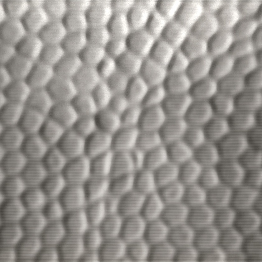
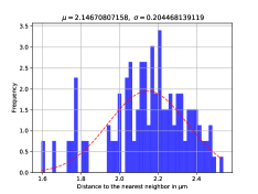
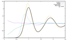
(a) 3-A

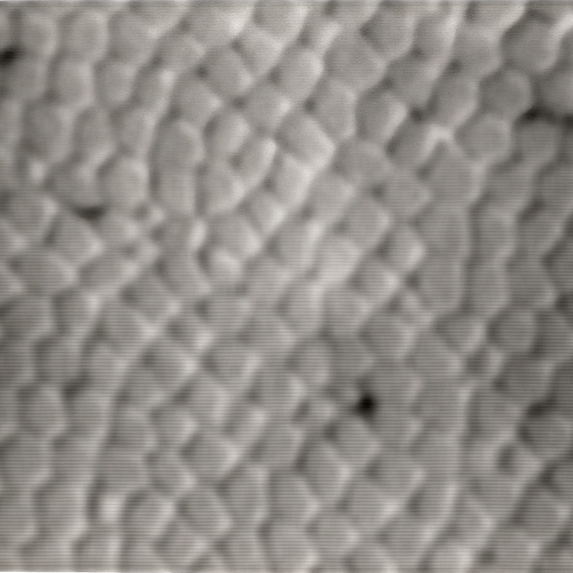
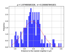
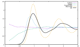
(b) 3-B

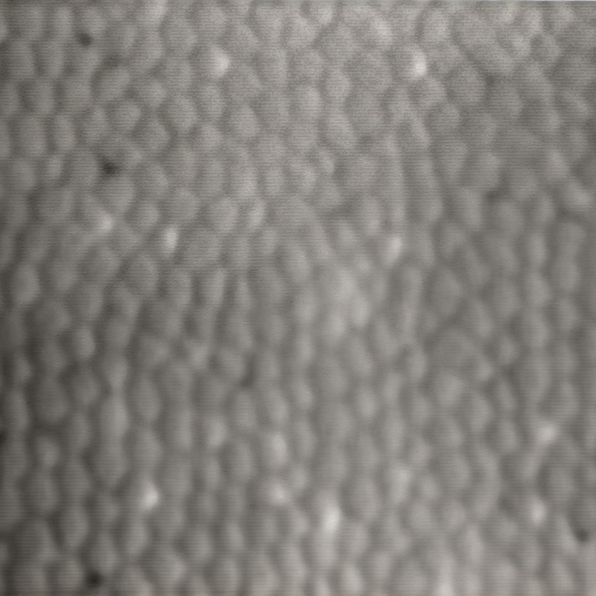
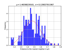
(c) 3-C

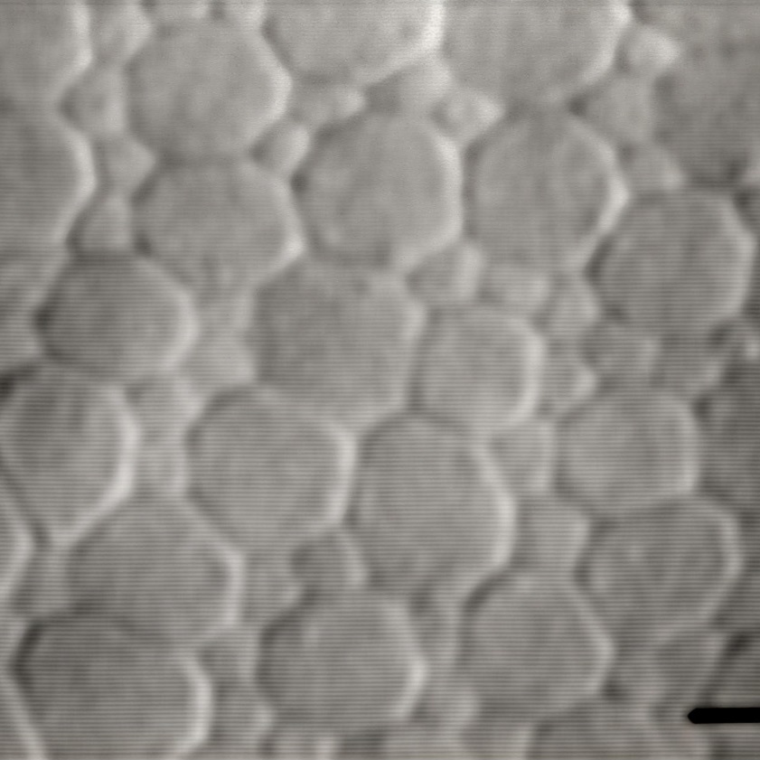
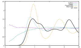
(d) 3-F

Figure 3: From left to right: The picture of the patch of retina, the point samples extracted from the cones’ location, Nearest neighbor analysis with mean and standard deviation, Pair Correlation Function. Images from Curcio et al.curcio1990human

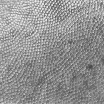
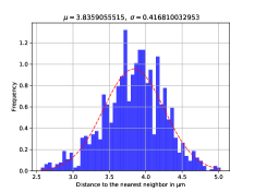
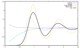
(a) 4-4

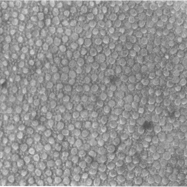
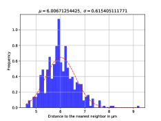
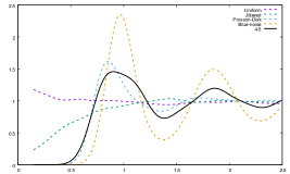
(b) 4-5

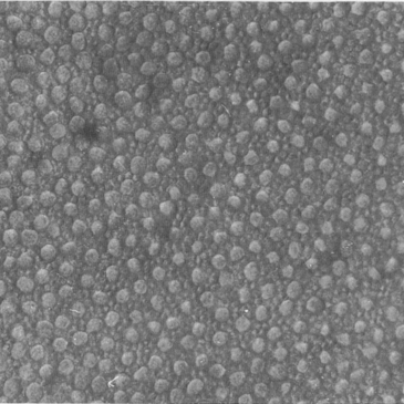
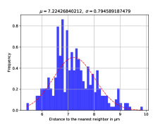
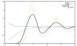
(c) 4-6

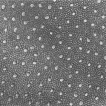
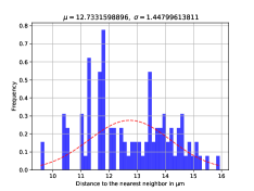
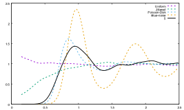
(d) 5

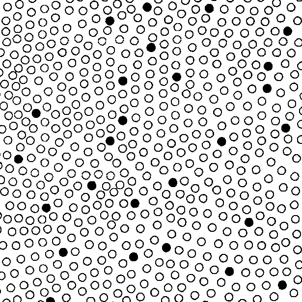
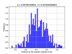
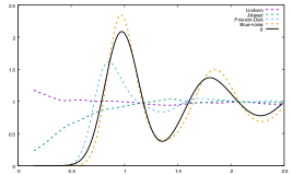
(e) 6

Figure 4: From left to right: The picture of the patch of retina, the point samples extracted from the cones’ location, Nearest neighbor analysis with mean and standard deviation, Pair Correlation Function. a-d. Images from Jonas et al. jonas1992count e. Image from Curcio et al. curcio1991distribution

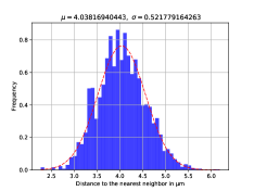
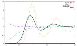
(a) 7-A

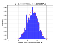
(b) 7-B

Figure 5: From left to right: The picture of the patch of retina, the point samples extracted from the cones’ location, Nearest neighbor analysis with mean and standard deviation, Pair Correlation Function. Images from Curcio et al. curcio1991distribution

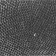
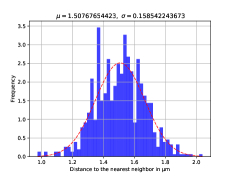
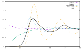
(a) 8-G

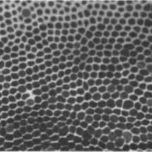
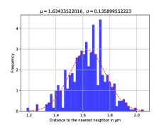
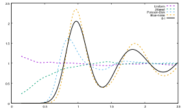
(b) 8-I

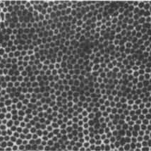
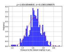
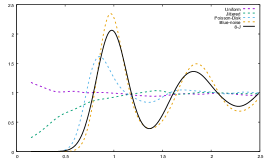
(c) 8-J

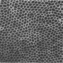
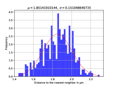
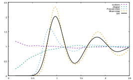
(d) 8-K

Figure 6: From left to right: The picture of the patch of retina, the point samples extracted from the cones’ location, Nearest neighbor analysis with mean and standard deviation, Pair Correlation Function. Images from Gao & Hollyfield gao1992aging

A more recent and reliable method for assessing the goodness of these processes is the previously mentioned Pair Correlation Function. In Table 2, we present the $l_{\infty}$ distance, between our generated point sets and the measured PCF. From two PCFs $\varrho$ and $\varrho_{2}$, we denote their $l_{\infty}$ distance as the maximal distance between the two functions:

$$l_{\infty}(\varrho,\varrho_{2})=max_{r}|\varrho(r)-\varrho_{2}(r)|\,,$$ (5)

where $r$ is a given radius. We rely on this measure as it was already used in Oztireli2012 to compare PCFs, two distributions can be considered the same if this difference is under 0.1. The closest results are from comparison with BNOT and Dart Throwing samplers, moreover, the higher the measured RI for the retinal distribution of photoreceptors, the lower the distance from BNOT PCF. The opposite happens when comparing with Dart throwing algorithm, the closer to the reported RI of 8, the lower the $l_{\infty}$ distance. This evidences that not only the indexes are actually higher than the ones previously measured, but also that the most effective method to simulate these distributions comes from Blue-noise samplers.

Table 2: $l_{\infty}$ distances between pairs of PCFs. If this difference is under 0.1, the two distribution can be considered to be the same. It is clearly visible that the Dart Throwing and BNOT samplers are the closest from the measured distribution.

Data	BNOT 1024	DT 1024	Jitter 1024
1-A	0.507644	0.525371	0.945527
1-F	0.52156	0.566554	0.912223
1-G	0.778872	0.309411	0.663769
2-A	0.298435	0.764314	1.13442
3-A	0.408852	0.851508	1.1428
3-B	0.549172	0.518775	0.886055
3-C	0.484184	0.597551	0.948338
3-D	0.401644	1.1555	1.41747
3-F	0.856925	0.484083	0.633278
4-4	0.472629	0.598528	0.959664
4-5	0.917283	0.262972	0.597261
4-6	0.642895	0.525127	0.806347
5	0.920215	0.383484	0.578448
6	0.264755	0.809063	1.1713
7-A	0.778203	0.248315	0.761941
7-B	0.803054	0.245291	0.686117
8-G	0.826069	0.331142	0.638697
8-I	0.301428	0.768822	1.13356
8-J	0.297661	0.797065	1.14651
8-K	0.327341	0.737896	1.10608

5 Conclusions

Blue noise sampling can describe features of a human retinal cone distribution with a certain degree of similarity to the available data and can be efficiently used for modeling local patches of retina. We hope this work can be useful to understand how spatial distribution affects the sampling of a retinal image, or the mechanisms underlying the development of this singular distribution of neuron cells and the implications it has on human vision. Given the nature of blue-noise algorithms, it should be possible to develop an adaptive sampling model that spans the whole retina. However, there would be issues in validating the cone sampling, since imaging of the whole retina is difficult to obtain and analyze. All validation in fact should also be local. Future works will explore the possibility of applying a smooth sampling across the retina to obtain an adaptive sampling, given the PCF and spectra of local patches, the patches can be reproduced zhou2012point and correlated with a heat map that represents interpolation in space roveri2017general .

References

- (1) Ahmed, A., Niese, T., Huang, H., Deussen, O.: An adaptive point sampler on a regular lattice. ACM Trans. Graph. 36(4), 138:1–138:13 (2017)
- (2) Ahmed, A., Perrier, H., Coeurjolly, D., Ostromoukhov, V., Guo, J., Dongming Yan, H.H., Deussen, O.: Low-discrepancy blue noise sampling. ACM Transactions on Graphics (Proceedings of ACM SIGGRAPH Asia 2016) 35(6), 247:1–247:13 (2016)
- (3) Ahmed, A.G., Huang, H., Deussen, O.: Aa patterns for point sets with controlled spectral properties. ACM Transactions on Graphics (TOG) 34(6), 212 (2015)
- (4) Ahumada Jr, A.J., Poirson, A.: Cone sampling array models. JOSA A 4(8), 1493–1502 (1987)
- (5) Balzer, M., Schlömer, T., Deussen, O.: Capacity-constrained point distributions: A variant of Lloyd’s method. ACM Trans. Graph. 28(3), 86:1–8 (2009)
- (6) Bowers, J., Wang, R., Wei, L.Y., Maletz, D.: Parallel Poisson disk sampling with spectrum analysis on surfaces. ACM Trans. Graph. 29, 166:1–166:10 (2010)
- (7) Bridson, R.: Fast Poisson disk sampling in arbitrary dimensions. In: ACM SIGGRAPH sketches (2007). DOI http://doi.acm.org/10.1145/1278780.1278807. URL http://doi.acm.org/10.1145/1278780.1278807
- (8) Chen, Z., Yuan, Z., Choi, Y.K., Liu, L., Wang, W.: Variational blue noise sampling. IEEE Transactions on Visualization and Computer Graphics 18(10), 1784–1796 (2012)
- (9) Cohen, M.F., Shade, J., Hiller, S., Deussen, O.: Wang tiles for image and texture generation. In: ACM SIGGRAPH, pp. 287–294 (2003). DOI http://doi.acm.org/10.1145/1201775.882265. URL http://doi.acm.org/10.1145/1201775.882265
- (10) Cook, J.: Spatial properties of retinal mosaics: an empirical evaluation of some existing measures. Visual neuroscience 13(1), 15–30 (1996)
- (11) Cook, R.L.: Stochastic sampling in computer graphics. ACM Trans. Graph. 5(1), 51–72 (1986)
- (12) Crow, F.C.: The aliasing problem in computer-generated shaded images. Commun. ACM 20(11), 799–805 (1977)
- (13) Curcio, C.A., Allen, K.A., Sloan, K.R., Lerea, C.L., Hurley, J.B., Klock, I.B., Milam, A.H.: Distribution and morphology of human cone photoreceptors stained with anti-blue opsin. Journal of Comparative Neurology 312(4), 610–624 (1991)
- (14) Curcio, C.A., Sloan, K.R.: Packing geometry of human cone photoreceptors: variation with eccentricity and evidence for local anisotropy. Visual neuroscience 9(2), 169–180 (1992)
- (15) Curcio, C.A., Sloan, K.R., Kalina, R.E., Hendrickson, A.E.: Human photoreceptor topography. Journal of comparative neurology 292(4), 497–523 (1990)
- (16) Deering, M.F.: A human eye retinal cone synthesizer. In: ACM SIGGRAPH 2005 Sketches, p. 128. ACM (2005)
- (17) Dees, E.W., Dubra, A., Baraas, R.C.: Variability in parafoveal cone mosaic in normal trichromatic individuals. Biomedical optics express 2(5), 1351–1358 (2011)
- (18) Dippé, M.A.Z., Wold, E.H.: Antialiasing through stochastic sampling. In: ACM SIGGRAPH, pp. 69–78 (1985)
- (19) Drasdo, N., Fowler, C.: Non-linear projection of the retinal image in a wide-angle schematic eye. The British journal of ophthalmology 58(8), 709 (1974)
- (20) Dunbar, D., Humphreys, G.: A spatial data structure for fast Poisson-disk sample generation. ACM Trans. Graph. 25(3), 503–508 (2006)
- (21) Dunbar, D., Humphreys, G.: A spatial data structure for fast poisson-disk sample generation. ACM Trans. Graph. 25(3), 503–508 (2006)
- (22) Ebeida, M.S., Davidson, A.A., Patney, A., Knupp, P.M., Mitchell, S.A., Owens, J.D.: Efficient maximal Poisson-disk sampling. ACM Trans. Graph. 30, 49:1–49:12 (2011). DOI http://doi.acm.org/10.1145/2010324.1964944. URL http://doi.acm.org/10.1145/2010324.1964944
- (23) Ebeida, M.S., Mitchell, S.A., Patney, A., Davidson, A.A., Owens, J.D.: A simple algorithm for maximal poisson-disk sampling in high dimensions. Comp. Graph. Forum 31(2pt4), 785–794 (2012)
- (24) Eglen, S.J.: Cellular spacing: Analysis and modelling of retinal mosaics. In: Computational Systems Neurobiology, pp. 365–385. Springer (2012)
- (25) Fattal, R.: Blue-noise point sampling using kernel density model. ACM Trans. Graph. 30(3), 48:1–48:12 (2011)
- (26) Floyd, R.W., Steinberg, L.: An adaptive algorithm for spatial grey scale. Proc. Soc. Inf. Display 17, 75–77 (1976)
- (27) Galli-Resta, L., Novelli, E., Kryger, Z., Jacobs, G., Reese, B.: Modelling the mosaic organization of rod and cone photoreceptors with a minimal-spacing rule. European Journal of Neuroscience 11(4), 1461–1469 (1999)
- (28) Gamito, M.N., Maddock, S.C.: Accurate multidimensional Poisson-disk sampling. ACM Trans. Graph. 29, 8:1–8:19 (2009)
- (29) Gamito, M.N., Maddock, S.C.: Accurate multidimensional poisson-disk sampling. ACM Transactions on Graphics (TOG) 29(1), 8 (2009)
- (30) Gao, H., Hollyfield, J.: Aging of the human retina. differential loss of neurons and retinal pigment epithelial cells. Investigative ophthalmology & visual science 33(1), 1–17 (1992)
- (31) de Goes, F., Breeden, K., Ostromoukhov, V., Desbrun, M.: Blue noise through optimal transport. ACM Trans. Graph. 31(6), 171:1–171:11 (2012)
- (32) Heck, D., Schlömer, T., Deussen, O.: Blue noise sampling with controlled aliasing. ACM Trans. Graph. 32(3), 25:1–25:12 (2013)
- (33) Hofer, H., Singer, B., Williams, D.R.: Different sensations from cones with the same photopigment. Journal of Vision 5(5), 5–5 (2005)
- (34) Illian, J., Penttinen, A., Stoyan, H., Stoyan, D.: Statistical analysis and modelling of spatial point patterns, vol. 70. John Wiley & Sons (2008)
- (35) Jonas, J.B., Schneider, U., Naumann, G.O.: Count and density of human retinal photoreceptors. Graefe’s Archive for Clinical and Experimental Ophthalmology 230(6), 505–510 (1992)
- (36) Jones, T.R.: Efficient generation of Poisson-disk sampling patterns. Journal of Graphics, GPU, & Game Tools 11(2), 27–36 (2006)
- (37) Kopf, J., Cohen-Or, D., Deussen, O., Lischinski, D.: Recursive Wang tiles for real-time blue noise. ACM Trans. Graph. 25(3), 509–518 (2006)
- (38) Lagae, A.: Wang tiles in computer graphics. Synthesis Lectures on Computer Graphics and Animation 4(1), 1–91 (2009)
- (39) Lagae, A., Dutré, P.: An Alternative for Wang Tiles: Colored Edges versus Colored Corners. ACM Trans. Graph., 25(4), 1442–1459 (2006)
- (40) Lagae, A., Dutré, P.: A comparison of methods for generating poisson disk distributions. Computer Graphics Forum 27(1), 114–129 (2008)
- (41) McCool, M., Fiume, E.: Hierarchical Poisson disk sampling distributions. In: Proc. Graphics Interface ’92, pp. 94–105 (1992)
- (42) Mitchell, D.: Spectrally optimal sampling for distributed ray tracing. In: Proc. SIGGRAPH ’91, vol. 25, pp. 157–164 (1991)
- (43) Mitchell, D.P.: Generating antialiased images at low sampling densities. In: ACM SIGGRAPH, pp. 65–72 (1987)
- (44) Morillas, C., Pelayo, F., et al.: A conductance-based neuronal network model for color coding in the primate foveal retina. In: International Work-Conference on the Interplay Between Natural and Artificial Computation, pp. 63–74. Springer (2017)
- (45) Morillas, C., Pino, B., Pelayo, F., et al.: Towards a generic simulation tool of retina models. In: International Work-Conference on the Interplay Between Natural and Artificial Computation, pp. 47–57. Springer (2015)
- (46) Ostromoukhov, V.: Sampling with polyominoes. ACM Trans. Graph. 26(3), 78:1–78:6 (2007)
- (47) Ostromoukhov, V., Donohue, C., Jodoin, P.M.: Fast hierarchical importance sampling with blue noise properties. ACM Trans. Graph. 23(3), 488–495 (2004)
- (48) Öztireli, A.C., Gross, M.: Analysis and synthesis of point distributions based on pair correlation. ACM Trans. Graph. (Proc. of ACM SIGGRAPH ASIA) 31(6), to appear (2012)
- (49) Reinert, B., Ritschel, T., Seidel, H.P., Georgiev, I.: Projective blue-noise sampling. Computer Graphics Forum 35(1), 285–295 (2016)
- (50) Rohatgi, A.: Webplotdigitizer. URL http://arohatgi.info/WebPlotDigitizer/app (2011)
- (51) Roorda, A., Williams, D.R.: The arrangement of the three cone classes in the living human eye. Nature 397(6719), 520–522 (1999)
- (52) Roveri, R., Öztireli, A.C., Gross, M.: General point sampling with adaptive density and correlations. In: Computer Graphics Forum, vol. 36, pp. 107–117. Wiley Online Library (2017)
- (53) Schlömer, T., Heck, D., Deussen, O.: Farthest-point optimized point sets with maximized minimum distance. In: Symp. on High Performance Graphics, pp. 135–142 (2011)
- (54) Schmaltz, C., Gwosdek, P., Bruhn, A., Weickert, J.: Electrostatic halftoning. Comput. Graph. Forum 29(8), 2313–2327 (2010)
- (55) Scoles, D., Sulai, Y.N., Langlo, C.S., Fishman, G.A., Curcio, C.A., Carroll, J., Dubra, A.: In vivo imaging of human cone photoreceptor inner segmentsin vivo imaging of photoreceptor inner segments. Investigative ophthalmology & visual science 55(7), 4244–4251 (2014)
- (56) Shirley, P.: Discrepancy as a quality measure for sample distributions. In: Proc. Eurographics ’91, pp. 183–194 (1991)
- (57) Song, H., Chui, T.Y.P., Zhong, Z., Elsner, A.E., Burns, S.A.: Variation of cone photoreceptor packing density with retinal eccentricity and age. Investigative ophthalmology & visual science 52(10), 7376–7384 (2011)
- (58) Ulichney, R.: Digital Halftoning. MIT Press (1987)
- (59) Wachtel, F., Pilleboue, A., Coeurjolly, D., Breeden, K., Singh, G., Cathelin, G., de Goes, F., Desbrun, M., Ostromoukhov, V.: Fast tile-based adaptive sampling with user-specified Fourier spectra. ACM Trans. Graph. 33(4) (2014)
- (60) Wang, Y.Z., Thibos, L.N., Bradley, A.: Modeling the sampling properties of human cone photoreceptor mosaic. In: Vision Science and its Applications, p. FB1. Optical Society of America (2001)
- (61) Wassle, H., Riemann, H.: The mosaic of nerve cells in the mammalian retina. Proceedings of the Royal Society of London B: Biological Sciences 200(1141), 441–461 (1978)
- (62) Wei, L.Y.: Parallel Poisson disk sampling. ACM Trans. Graph. (SIGGRAPH) 27, 20:1–20:9 (2008)
- (63) Wohrer, A., Kornprobst, P.: Virtual retina: a biological retina model and simulator, with contrast gain control. Journal of computational neuroscience 26(2), 219–249 (2009)
- (64) Wong, K.S., Jian, Y., Cua, M., Bonora, S., Zawadzki, R.J., Sarunic, M.V.: In vivo imaging of human photoreceptor mosaic with wavefront sensorless adaptive optics optical coherence tomography. Biomedical optics express 6(2), 580–590 (2015)
- (65) Wyszecki, G., Stiles, W.S.: Color science. Concepts and Methods, Quantitative Data and Formulae, 2nd Edition, vol. 8. Wiley New York (1982)
- (66) Xiang, Y., Xin, S.Q., Sun, Q., He, Y.: Parallel and accurate Poisson disk sampling on arbitrary surfaces. In: SIGGRAPH Asia Sketches, pp. 18:1–18:2 (2011)
- (67) Yellott, J.I.: Spectral consequences of photoreceptor sampling in the rhesus retina. Science 221(4608) (1983)
- (68) Zhou, Y., Huang, H., Wei, L.Y., Wang, R.: Point sampling with general noise spectrum. ACM Trans. Graph. 31(4), 76:1–76:11 (2012)
- (69) Zhou, Y., Huang, H., Wei, L.Y., Wang, R.: Point sampling with general noise spectrum. ACM Transactions on Graphics (TOG) 31(4), 76 (2012)