Coordinate independent approach to the calculation of the effects of local structure on the luminosity distance

Abstract

Local structure can have important effects on luminosity distance observations, which could for example affect the local estimation of the Hubble constant based on low red-shift type Ia supernovae.

Using a spherically symmetric exact solution of the Eistein’s equations and a more accurate expansion of the solution of the geodesic equations, we improve the low red-shift expansion of the monopole of the luminosity distance in terms of the curvature function. Based on this we derive the coordinate independent low red-shift expansion of the monopole of the luminosity distance in terms of the monopole of the density contrast. The advantage of this approach is that it relates the luminosity distance directly to density observations, without any dependency on the radial coordinate choice.

We compute the effects of different inhomogeneities on the luminosity distance, and find that the formulae in terms of the density contrast are in good agreement with numerical calculations, in the non linear regime are more accurate than the results obtained using linear perturbation theory, and are also more accurate than the formulae in terms of the curvature function.

I Introduction

The luminosity distance is an observable quantity of fundamental importance for modern Cosmology, and it provided the first evidence of dark energy Perlmutter:1998np ; Riess:1998cb , i.e. the late time accelerated expansion of the Universe. Low red-shift luminosity distance observations Riess:2016jrr ; Riess:2018byc ; Riess:2019cxk are also used to determine the Hubble constant $H_{0}$ under the assumption of spatial homogeneity, but the value of $H_{0}$ obtained from local measurements is in disagreement with the value inferred from CMB observations Riess:2016jrr ; Riess:2018byc ; Ade:2015xua ; Aghanim:2018eyx ; Riess:2019cxk . The discrepancy has been recently claimed to be of order $4.4\sigma$ tension Riess:2019cxk .

The unaccounted effects of local structure on the luminosity distance could resolve this tension as shown for example in Romano:2014iea , and it is therefore important to study these effects. This motivates the calculation of low red-shift expansions for the luminosity distance based on using inhomogeneous exact solutions of Einstein’s field equations. The cosmological effects of inhomogeneities on different observables have been studied in Romano:2014iea ; Romano:2013kua ; Clarkson:2010ej ; Romano:2006yc ; Romano:2009xw ; Ben-Dayan:2014swa ; Redlich:2014gga ; Romano:2009qx ; EneaRomano:2011aa ; Marra:2011ct ; Romano:2011mx ; Romano:2010nc ; Krasinski:2014zza ; Romano:2012yq ; Romano:2012ks ; Balcerzak:2013kha ; Romano:2012gk ; 2012GReGr..44..353R ; Fanizza:2013doa ; RomanoChen:2014 ; Krasinski:2014lna ; Romano:2014tya ; Marra:2013rba ; Romano:2015iwa ; Vallejo:2017rga ; Chung:2006xh , and examples include the expansion scalar Romano:2015iwa , number counts, Vallejo:2017rga and the luminosity distance Romano:2010nc ; Romano:2012gk ; Romano:2011mx ; Chung:2006xh . In this paper we focus on the effects on the luminosity distance produced by the monopole of local structure modeled by a spherically symmetric solution of Einstein’s equations in presence of the cosmological constant.

A low red-shift expansion for the monopole of the luminosity distance was derived in Romano:2012gk in terms of the curvature function, and in this paper we improve these formulae by using a more accurate expansion of the solution of the geodesic equations Romano:2015iwa . We then use these formulae to derive a new coordinate independent low red-shift expansion for the luminosity distance in terms of the monopole of the density field. We compare the analytic results to exact numerical computations and perturbation theory Romano:2016utn , finding that the formulae in terms of the density contrast are in good agreement with the numerical results and more accurate than the formulae in terms of the curvature function and the perturbative calculation.

II Modeling the local Universe

We model the monopole component of the local structure using the Lemaître-Tolman-Bondi (LTB) metric Lemaitre:1933 ; Lemaitre:1933qeLemai ; Lemaitre:1931zz ; Tolman:1934za ; Bondi:1947av

$$ds^{2}=-dt^{2}+\frac{R^{\prime}(t,r)^{2}}{1+2\,E(r)}dr^{2}+R(t,r)^{2}d\Omega^{2}\,,$$ (1)

where $R$ is a function of the time coordinate $t$ and the radial coordinate $r$, $E(r)$ is an arbitrary function of $r$, $R^{\prime}(t,r)=\partial_{r}R(t,r)$, and we choose a system of units in which $c=8\pi G=1$. The Einstein’s equations imply

$$\left({\frac{\dot{R}}{R}}\right)^{2} = \frac{2E(r)}{R^{2}}+\frac{2M(r)}{R^{3}}+\frac{\Lambda}{3}\,,$$ (2)

$$\rho(t,r) = \frac{2M^{\prime}}{R^{2}R^{\prime}}\,,$$ (3)

where $M(r)$ is an arbitrary function of $r$ and $\dot{R}(t,r)=\partial_{t}R(t,r)$. The luminosity distance in a LTB space-time is given by

$$D_{L}(z) = (1+z)^{2}R(t(z),r(z))\,,$$ (4)

where $t(z)$ and $r(z)$ are the radial null geodesics, which are obtained by solving the geodesic equations Celerier:1999hp

$$\frac{dr}{dz} = \frac{\sqrt{1+2E(r(z))}}{(1+z)\dot{R^{\prime}}[t(z),r(z)]}\,,$$ (5)

$$\frac{dt}{dz} = -\,\frac{R^{\prime}[t(z),r(z)]}{(1+z)\dot{R^{\prime}}[t(z),r(z)]}\,.$$ (6)

The analytical solution of eq.(2) can be derived Zecca:2013wda ; Edwards01081972 introducing a new coordinate $\eta=\eta(t,r)$, and new functions $\rho_{0}(r)$ and $k(r)$ given by

$$\frac{\partial\eta}{\partial t}|_{r} = \frac{r}{R}=\frac{1}{a}\,,$$ (7)

$$\rho_{0}(r) = \frac{6M(r)}{r^{3}}\,,$$ (8)

$$k(r) = -\frac{2E(r)}{r^{2}}\,.$$ (9)

We will adopt, without loss of generality, the coordinate system in which $\rho_{0}(r)$ is a constant, the so called FLRW gauge. We can express eq.(2) in the form

$$\left(\frac{\partial a}{\partial\eta}\right)^{2}=-k(r)a^{2}+\frac{\rho_{0}}{3}a+\frac{\Lambda}{3}a^{4}\,.$$ (10)

III Coordinate independent red-shift expansion of the luminosity distance

Our goal is to find an analytical formula for the luminosity distance in terms of the density contrast $\delta(z)$ at low red-shift. In order to derive the formula we take into account the metric reconstruction of the local Universe given in Vallejo:2017rga . We follow the same procedure described in sections III and IV of Vallejo:2017rga and we expand the curvature function $k(r)$ according to

$$k(r) =k_{0}+k_{1}r+k_{2}r^{2}+...\,.$$ (11)

In this section we derive the formulae for the case in which $k_{0}=0$, and report the general case in appendix B.

After expanding the luminosity distance in red-shift space we get

$$D_{L}(z) =D_{1}z+D_{2}z^{2}+D_{3}z^{3}\,,$$ (12)

$$D_{1} =\frac{1}{H_{0}},$$ (13)

$$D_{2} =\frac{4-6\alpha K_{1}\Omega_{M}-3\Omega_{M}}{4H_{0}}\,,$$ (14)

$$D_{3} =\frac{1}{24H_{0}\Omega_{\Lambda}\Omega_{M}}\Big{\{}-2K_{1}^{2}\big{[}2\zeta_{0}+3\Omega_{\Lambda}\Omega_{M}\left(4\alpha-3\alpha^{2}\Omega_{M}\left(6\Omega_{M}-5\right)+3\beta\Omega_{M}\right)-2\big{]}+$$

$$\quad{}+4K_{1}\Omega_{\Lambda}\Omega_{M}\big{[}27\alpha\Omega_{M}^{2}-24\alpha\Omega_{M}-2\big{]}+3\Omega_{\Lambda}\Omega_{M}^{2}\big{[}9\Omega_{M}-2\left(6\alpha K_{2}+5\right)\big{]}\Big{\}}\,,$$ (15)

where we have introduced the parameters $H_{0}$, $\Omega_{M}$, $\Omega_{\Lambda}$, $K_{n}$, $\alpha$, $\beta$, according to the definitions given in EneaRomano:2011aa ; Romano:2015iwa ; Vallejo:2017rga .

Note that the above formulae depend on the coordinates choice since the coefficients $D_{2}$ and $D_{3}$ given in eq.(14) and eq.(15) are expressed in terms of the coefficients $K_{1}$ and $K_{2}$, which depend on the choice of the radial coordinate $r$. It is also important to note that a similar expansion in terms of the curvature function was previously derived in Romano:2012gk . However, the formulae we have derived is based on a more accurate expansion of the solution of the geodesic equations Romano:2015iwa ; Vallejo:2017rga , and therefore are more precise than the previous formulae.

It is easy to check that the formulae have the correct dimensions since all the parameters are dimensionless except for $H_{0}$. The intermediate steps necessary to derive these expressions are rather cumbersome, for this reason the results are expressed in terms of the above mentioned parameters after making all the analytical calculations using complex simplifying routines written in Mathematica. This procedure facilitates the physical interpretation of the results and ensures an immediate check of the dimensional consistency.

As can be seen in eq.(14) the effects of the inhomogeneity start to show at second order in the red-shift expansion of the luminosity distance. Note that in absence of inhomogeneities, i.e. $K_{1}=K_{2}=0$ the obtained formulae reduce to the standard FLRW case.

We can now use the reconstructed metric given in Vallejo:2017rga to find the luminosity distance in terms of the density contrast. In order to do this we expand $\delta(z)$ as

$$\delta(z)=\delta_{0}+\delta_{1}z+\delta_{2}z^{2}\,,$$ (16)

and after replacing the expressions for $K_{1}$ and $K_{2}$ found in Vallejo:2017rga into eq.(14) and eq.(15) we get

$${}D_{2} =-\frac{2H_{0}^{2}\left(3\Omega_{M}-4\right)\left(3\alpha\Omega_{M}+1\right)+9\alpha\delta_{1}\overline{H}_{0}^{2}\overline{\Omega}_{M}\Omega_{M}}{8H_{0}^{3}\left(3\alpha\Omega_{M}+1\right)}\,,$$ (17)

$$D_{3} =\frac{1}{640H_{0}^{5}\Omega_{\Lambda}\Omega_{M}\left(3\alpha\Omega_{M}+1\right){}^{3}}\Big{\{}80H_{0}^{4}\Omega_{\Lambda}\Omega_{M}^{2}\left(9\Omega_{M}-10\right)\left(3\alpha\Omega_{M}+1\right){}^{3}+$$

$$\quad{}+3\overline{H}_{0}^{4}\overline{\Omega}_{M}^{2}\delta_{1}{}^{2}\big{[}-20\zeta_{0}+1377\alpha^{3}\Omega_{\Lambda}\Omega_{M}^{4}+30\Omega_{M}^{2}\left(3\alpha^{2}\Omega_{\Lambda}-2\alpha-3\beta\Omega_{\Lambda}\right)+$$

$$\quad{}+324\alpha^{2}\Omega_{\Lambda}\Omega_{M}^{3}+60\alpha\Omega_{M}+20\big{]}+8H_{0}^{2}\overline{H}_{0}^{2}\overline{\Omega}_{M}\Omega_{\Lambda}\Omega_{M}\left(3\alpha\Omega_{M}+1\right)\big{[}\delta_{1}\left(729\alpha^{2}\Omega_{M}^{3}+\right.$$

$$\quad{}\left.-72\alpha(10\alpha-3)\Omega_{M}^{2}-300\alpha\Omega_{M}-20\right)-72\alpha\delta_{2}\Omega_{M}\left(3\alpha\Omega_{M}+1\right)\big{]}\Big{\}}\,,$$ (18)

where the parameters $\overline{H}_{0}$ and $\overline{\Omega}_{M}$ are given in appendix A.

It is important to note that the above formulae for the luminosity distance in terms of the density contrast do not depend on the choice of radial coordinate. It is easy to check that the formulae reduce to the FLRW luminosity distance expansion in the homogeneous limit $\delta_{1}=\delta_{2}=0$.

IV Testing the accuracy of the Formulae

In order to compare our analytical formulae with numerical computations we consider inhomogeneities defined by the curvature function

$$k(r)=-\lambda H_{0}^{2}\frac{rH_{0}}{\nu^{2}}\left(2+\nu\,rH_{0}\right)\exp\left[-\left(\frac{rH_{0}}{\nu}\right)^{2}\right]\,,$$ (19)

which are shown in fig.(1). In order to compute the luminosity distance we first solve numerically the Einstein’s eq.(2) and the radial null geodesic equations given in eq.(5) and eq.(6), and then substitute the solutions of the geodesics equations in eq.(4). Since we are considering asymptotically flat compensated structures, the background is flat, $\overline{H}_{0}=H_{0}$ and $\overline{\Omega}_{M}=\Omega_{M}$.

In order to check if the structure is in the linear regime we can compute the corresponding curvature perturbation using the relation Romano:2010nc

$$\left[r\zeta^{\prime}(r)+1\right]^{2}=1-r^{2}k(r)\,,$$ (20)

and we plot in fig.(2) this quantity for the different inhomogeneities we consider.

Figure 1: The function $k(r)$ defined in eq.(19) is plotted in units of $H_{0}^{2}$ as a function of the radial coordinate for $\nu=2\times 10^{-1}$, $\lambda=5\times 10^{-4}$ (left) and $\nu=2\times 10^{-1}$, $\lambda=5\times 10^{-2}$ (right).

Figure 2: The curvature perturbation $\zeta(r)$ is plotted as a function of the radial coordinate in units of $H_{0}^{-1}$. The left and right plots correspond to the same models shown in fig.(1).

Figure 3: The density contrast $\delta(z)$ is plotted as a function of red-shift. The left and right plots correspond to the same models shown in fig.(1).

We also compare our formulae with the low red-shift perturbative approximation Romano:2016utn given by

$$D_{L}(z)=\overline{D}_{L}(z)\left[1+\frac{1}{3}f\overline{\delta}(z)\right]\,,$$ (21)

where

$$\overline{\delta}(z) =\frac{3}{\chi(z)^{3}}\int_{0}^{z}\frac{\chi(y)^{2}\delta(y)}{\overline{H}(y)}dy\,,$$ (22)

is the volume average of the density contrast over a sphere of comoving radius $\chi(z)$, $\chi$, $\overline{H}$ and $\overline{D}_{L}$ are the comoving distance, Hubble parameter and luminosity distance of the background Universe, and $f=\overline{\Omega}_{M}{}^{0.55}$ is the growth rate. We plot in fig.(3) the density contrast for the different models. As can be seen from fig.(5) the formula for the luminosity distance in terms of the curvature function coefficients $K_{1}$ and $K_{2}$ is not accurate compared to the formula in terms of the density contrast, which is also more accurate than perturbation theory.

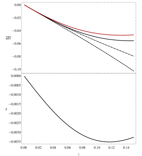
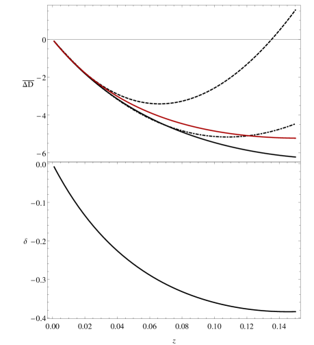
Figure 4: The relative percentual difference $\overline{\Delta D}=100(D_{L}/\overline{D}_{L}-1)$ is plotted as a function of red-shift. The black solid curve corresponds to the numerical solution, the dot-dashed curve to the coordinate independent formula in terms of the density contrast, the black dashed curve to the formula in terms of the curvature function expansion coefficients $K_{1}$ and $K_{2}$, and the red curve to the perturbative formula given in eq.(21). The left and right plots correspond to the same models shown in fig.(1). At the bottom the density contrast is plotted as a function of red-shift for the corresponding models.

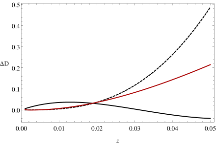
Figure 5: The relative percentual difference $\Delta D=100\left(D_{L}^{an}/D_{L}^{num}-1\right)$ is plotted as a function of red-shift. The black solid curve corresponds to the analytical formula given in terms of $\delta_{1}$ and $\delta_{2}$, the black dashed curve to the formula in terms of the curvature coefficients $K_{1}$ and $K_{2}$, and the red curve to the perturbative approximation given in eq.(21). The left and right plots correspond to the same models shown in fig.(1). As can be seen the coordinate independent formula is the one in best agreement with numerical results.

V Conclusions

We have computed an improved low red-shift formula of the luminosity distance in terms of the curvature function using a more accurate expansion of the solution of the geodesic equations. Based on this result we have derived for the first time a low red-shift expansion of the luminosity distance in terms of the density contrast. The advantage of this approach is that it allows to obtain coordinate independent formulae whose coefficients are directly related to density observations, contrary to previous calculations in which the coefficients were in terms of the curvature function, and were consequently also depending on the choice of the radial coordinate.

The formulae are in good agreement with numerical calculations and are more accurate than results obtained using perturbation theory. In the future it will be interesting to use the formulae to develop an inversion method to reconstruct the monopole of the density contrast from the monopole of the luminosity distance. The results of the inversion could be used to test the validity of the assumption of homogeneity used in the estimation of cosmological parameters, such as the Hubble constant, from local observations. It will also be interesting to adopt other expansion methods such as the Padé approximation. In order to consider the effects of higher multipoles of the local structure, other non spherically symmetric solutions of the Einstein’s equations could be used to obtain the low red-shift expansion of the luminosity distance.

Appendix A Definitions of background quantities

The sub-horizon volume average on constant time slices for any scalar $S(t,r)$ is defined as

$$\overline{S}(t) =\frac{\int S(t,r)dV(t)}{\int dV(t)}\,,$$ (23)

$$\int dV(t)= \int_{0}^{r_{h}(t)}\frac{R(t,r)^{2}R^{\prime}(t,r)}{\sqrt{1-k(r)r^{2}}}dr\,,$$ (24)

where $r_{h}(t)$ is the comoving horizon as a function of time. For compensated inhomogeneities, such as the ones we consider in this paper, the average $\overline{S}$ will is well approximated by the asymptotic value

$$\overline{S}(t)=\lim_{r\to\infty}S(t,r)\,.$$ (25)

For example the background Hubble constant $\overline{H}_{0}$ is obtained from the volume average of the LTB Hubble parameter defined in terms of the expansion scalar

$$H(t,r)=\frac{2\dot{R}(t,r)}{3R(t,r)}+\frac{\dot{R^{\prime}}(t,r)}{3R^{\prime}(t,r)}\,$$ (26)

evaluated at present time $t_{0}$, $\overline{H}_{0}\equiv\overline{H}(t_{0})$, where $t_{0}=t(\eta_{0},0)$.

The background parameter $\overline{\Omega}_{M}$ is defined in terms of the volume average of the density $\rho(t,r)$ according to

$$\overline{\Omega}_{M}\equiv\frac{\overline{\rho}(t_{0})}{3\overline{H}_{0}^{2}}\,.$$ (27)

Appendix B General formulae

The low red-shift formulae for the luminosity distance, both the coordinate dependent and coordinate independent, are given in this appendix for the more general case in which $k_{0}$ is different from zero. We have used the computer algebra system provided by the Wolfram Mathematica software to derive all the formulae. Since $D_{1}=H_{0}^{-1}$ is also true for the general case we only give here the expressions for the coefficients $D_{2}$ and $D_{3}$ for simplicity, which in terms of $K_{1}$ and $K_{2}$ are given by

$$D_{2} =\frac{1}{4H_{0}\left(4K_{0}^{3}-27\Omega_{\Lambda}\Omega_{M}^{2}\right)}\Big{\{}8K_{0}^{4}\left(2\alpha K_{1}+1\right)-18K_{0}\Omega_{M}\big{[}K_{1}\left(-2\zeta_{0}+6\alpha\Omega_{\Lambda}\Omega_{M}+2\right)+$$

$$\quad{}+3\Omega_{\Lambda}\Omega_{M}\big{]}+27\Omega_{\Lambda}\Omega_{M}^{2}\big{[}\left(6\alpha K_{1}+3\right)\Omega_{M}-4\big{]}-4K_{0}^{3}\big{[}K_{1}\left(6\alpha\Omega_{M}+T_{0}\right)+3\Omega_{M}-4\big{]}+$$

$$\quad{}+6K_{1}K_{0}^{2}\left(T_{0}\Omega_{M}-4\zeta_{0}\right)\Big{\}}\,,$$ (28)

$$D_{3} =\frac{1}{8H_{0}\left(4K_{0}^{3}-27\Omega_{M}^{2}\Omega_{\Lambda}\right){}^{2}}\bigg{\{}64K_{0}^{8}-64\left(K_{1}T_{0}+3\Omega_{M}-1\right)K_{0}^{7}+16\Big{[}K_{1}^{2}T_{0}^{2}-2K_{2}T_{0}+$$

$$\quad{}-4K_{1}\big{(}6\zeta_{0}+T_{0}\left(1-3\Omega_{M}\right)\big{)}+\Omega_{M}\left(9\Omega_{M}-10\right)\Big{]}K_{0}^{6}-4\Big{[}T_{0}\big{(}-48\zeta_{0}+3T_{0}\left(4\Omega_{M}+\right.$$

$$\quad{}\left.-1\right)-4\big{)}K_{1}^{2}+96\zeta_{0}\left(1-3\Omega_{M}\right)K_{1}+4\Omega_{M}\big{(}T_{0}\left(9\Omega_{M}-8\right)+8\big{)}K_{1}+12\big{(}18\Omega_{\Lambda}\Omega_{M}^{2}+$$

$$\quad{}+K_{2}\left(4\zeta_{0}-T_{0}\Omega_{M}\right)\big{)}\Big{]}K_{0}^{5}+12\Big{[}\big{(}48\zeta_{0}^{2}+4\left(T_{0}\left(3-12\Omega_{M}\right)+4\right)\zeta_{0}+$$

$$\quad{}+T_{0}\Omega_{M}\left(T_{0}\left(3\Omega_{M}-2\right)+11\right)\big{)}K_{1}^{2}+4\Omega_{M}\big{(}-2\zeta_{0}\left(9\Omega_{M}-8\right)-8\Omega_{\Lambda}+\Omega_{M}\left(9T_{0}\Omega_{\Lambda}+\right.$$

$$\quad{}\left.+6\right)-4\big{)}K_{1}+24\Omega_{M}\big{(}K_{2}\left(\zeta_{0}-1\right)+3\Omega_{M}\left(3\Omega_{M}-1\right)\Omega_{\Lambda}\big{)}\Big{]}K_{0}^{4}+36\Big{[}\big{(}\left(12+\right.$$

$$\quad{}\left.-48\Omega_{M}\right)\zeta_{0}^{2}+2\Omega_{M}\left(T_{0}\left(6\Omega_{M}-4\right)+9\right)\zeta_{0}+\Omega_{M}\left(T_{0}\left(-7\Omega_{M}+3\Omega_{\Lambda}+3\right)+12\right)\big{)}K_{1}^{2}+$$

$$\quad{}+4\big{(}18\zeta_{0}+T_{0}\left(3-9\Omega_{M}\right)+2\big{)}\Omega_{M}^{2}\Omega_{\Lambda}K_{1}+6\Omega_{M}^{2}\big{(}K_{2}T_{0}+\left(10-9\Omega_{M}\right)\Omega_{M}\big{)}\Omega_{\Lambda}\Big{]}K_{0}^{3}+$$

$$\quad{}+108\Omega_{M}\Big{[}\big{(}4\left(3\Omega_{M}-2\right)\zeta_{0}^{2}+\left(-14\Omega_{M}+6\Omega_{\Lambda}+6\right)\zeta_{0}+\Omega_{M}\left(T_{0}\Omega_{\Lambda}+4\right)\big{)}K_{1}^{2}+$$

$$\quad{}+\Omega_{M}\big{(}\zeta_{0}\left(24-72\Omega_{M}\right)+\Omega_{M}\left(T_{0}\left(9\Omega_{M}-8\right)+8\right)\big{)}\Omega_{\Lambda}K_{1}+3\Omega_{M}\Omega_{\Lambda}\big{(}9\Omega_{\Lambda}\Omega_{M}^{2}+$$

$$\quad{}+K_{2}\left(4\zeta_{0}-T_{0}\Omega_{M}\right)\big{)}\Big{]}K_{0}^{2}+2\Big{[}\alpha^{2}\big{(}18\Omega_{M}^{2}-3\left(8K_{0}+5\right)\Omega_{M}+8K_{0}\left(K_{0}+1\right)\big{)}K_{1}^{2}+$$

$$\quad{}+\left(\beta K_{1}^{2}+2\alpha K_{2}\right)\left(2K_{0}-3\Omega_{M}\right)\Big{]}\left(4K_{0}^{3}-27\Omega_{M}^{2}\Omega_{\Lambda}\right){}^{2}-324\Omega_{M}^{2}\Omega_{\Lambda}\Big{[}\left(T_{0}\Omega_{M}-3\right)K_{1}^{2}+$$

$$\quad{}-2\Omega_{M}\big{(}-3\Omega_{M}+\zeta_{0}\left(9\Omega_{M}-8\right)+4\Omega_{\Lambda}+2\big{)}K_{1}+3\Omega_{M}\big{(}2K_{2}\left(\zeta_{0}-1\right)+3\Omega_{M}\left(3\Omega_{M}+\right.$$

$$\quad{}\left.-1\right)\Omega_{\Lambda}\big{)}\Big{]}K_{0}+243\Omega_{M}^{3}\Omega_{\Lambda}\Big{[}-4\left(\zeta_{0}-1\right)K_{1}^{2}-8\Omega_{M}\Omega_{\Lambda}K_{1}+3\Omega_{M}^{2}\left(9\Omega_{M}-10\right)\Omega_{\Lambda}\Big{]}+$$

$$\quad{}+4\alpha K_{1}\left(4K_{0}^{3}-27\Omega_{M}^{2}\Omega_{\Lambda}\right)\Big{[}16K_{0}^{5}-8\left(K_{1}T_{0}+6\Omega_{M}-2\right)K_{0}^{4}+4\big{(}\Omega_{M}\left(9\Omega_{M}-8\right)+$$

$$\quad{}+K_{1}\left(-12\zeta_{0}+T_{0}\left(6\Omega_{M}-2\right)-1\right)\big{)}K_{0}^{3}-3\big{(}36\Omega_{\Lambda}\Omega_{M}^{2}+K_{1}\{\zeta_{0}\left(16-48\Omega_{M}\right)+$$

$$\quad{}+\Omega_{M}[T_{0}\left(6\Omega_{M}-5\right)+4]\}\big{)}K_{0}^{2}-18\Omega_{M}\big{(}6\left(1-3\Omega_{M}\right)\Omega_{M}\Omega_{\Lambda}+K_{1}\left(-2\Omega_{M}+\right.$$

$$\quad{}\left.+\zeta_{0}\left(6\Omega_{M}-5\right)+3\Omega_{\Lambda}+1\right)\big{)}K_{0}+27\Omega_{M}^{2}\left(2K_{1}+\left(8-9\Omega_{M}\right)\Omega_{M}\right)\Omega_{\Lambda}\Big{]}\bigg{\}}\,.$$ (29)

The coordinate independent coefficients $D_{2}$ and $D_{3}$ are given by

$$D_{2} =\frac{1}{8H_{0}^{3}\Omega_{M}\mathcal{A}}\bigg{\{}\delta_{1}\overline{H}_{0}^{2}\overline{\Omega}_{M}\Big{[}-8\alpha K_{0}^{4}+18K_{0}\Omega_{M}\left(-\zeta_{0}+3\alpha\Omega_{\Lambda}\Omega_{M}+1\right)+2K_{0}^{3}\left(6\alpha\Omega_{M}+\right.$$

$$\quad{}\left.+T_{0}\right)+3K_{0}^{2}\left(4\zeta_{0}-T_{0}\Omega_{M}\right)-81\alpha\Omega_{\Lambda}\Omega_{M}^{3}\Big{]}+2H_{0}^{2}\Omega_{M}\left(2K_{0}-3\Omega_{M}+4\right)\mathcal{A}\bigg{\}}\,,$$ (30)

$$D_{3} =-\frac{1}{640H_{0}^{5}\Omega_{M}^{2}\mathcal{A}{}^{3}}\Bigg{\{}\overline{\Omega}_{M}^{2}\delta_{1}^{2}\bigg{[}4352\alpha^{3}K_{0}^{11}-64\alpha^{2}\big{(}51T_{0}+4\left(51\Omega_{M}\alpha+5\alpha+6\right)\big{)}K_{0}^{10}+$$

$$\quad{}+16\Big{(}\alpha\big{\{}51T_{0}^{2}+12\left(51\Omega_{M}\alpha+5\alpha+4\right)T_{0}+4\alpha[-306\zeta_{0}+9\Omega_{M}\left(17\alpha\Omega_{M}+16\right)+$$

$$\quad{}+40]\big{\}}-40\beta\Big{)}K_{0}^{9}-4\Big{(}17T_{0}^{3}+12\left(51\Omega_{M}\alpha+5\alpha+2\right)T_{0}^{2}+4\alpha\big{\{}-612\zeta_{0}+$$

$$\quad{}+9\Omega_{M}\left(51\alpha\Omega_{M}+32\right)+80\big{\}}T_{0}-720\beta\Omega_{M}+16\alpha\big{\{}-18\zeta_{0}\left(51\Omega_{M}\alpha+5\alpha+4\right)+$$

$$\quad{}+9\alpha\Omega_{M}[30\Omega_{M}+3\left(51\alpha\Omega_{M}+4\right)\Omega_{\Lambda}+34]+25\big{\}}\Big{)}K_{0}^{8}+4\Big{(}\left(51\Omega_{M}+5\right)T_{0}^{3}+$$

$$\quad{}+\big{\{}-306\zeta_{0}+9\Omega_{M}\left(51\alpha\Omega_{M}+16\right)+50\big{\}}T_{0}^{2}+4\big{\{}-36\zeta_{0}\left(51\Omega_{M}\alpha+5\alpha+2\right)+$$

$$\quad{}+9\alpha\Omega_{M}[60\Omega_{M}+6\left(51\alpha\Omega_{M}+4\right)\Omega_{\Lambda}+73]+25\big{\}}T_{0}-720\beta\Omega_{M}\left(\Omega_{M}+\Omega_{\Lambda}-1\right)+$$

$$\quad{}+24\alpha\big{\{}54\alpha\left(51\alpha\Omega_{\Lambda}+2\right)\Omega_{M}^{3}+9\alpha[-51\zeta_{0}+6(5\alpha+8)\Omega_{\Lambda}+29]\Omega_{M}^{2}+\left(90\alpha-288\zeta_{0}+\right.$$

$$\quad{}\left.+137\right)\Omega_{M}+2\zeta_{0}\left(153\zeta_{0}-40\right)\big{\}}\Big{)}K_{0}^{7}-3\Big{(}66096\alpha^{3}\Omega_{\Lambda}\Omega_{M}^{4}+864\alpha\big{\{}54\alpha\Omega_{\Lambda}+$$

$$\quad{}+T_{0}\left(51\alpha\Omega_{\Lambda}+2\right)\big{\}}\Omega_{M}^{3}+3\big{\{}17T_{0}^{3}+12\left(51\alpha\Omega_{\Lambda}+10\right)T_{0}^{2}+16\alpha[-153\zeta_{0}+18(5\alpha+$$

$$\quad{}+6)\Omega_{\Lambda}+92]T_{0}+3296\alpha-288[5(\beta-3\alpha^{2})\Omega_{\Lambda}+2\alpha\zeta_{0}\left(51\alpha\Omega_{\Lambda}+10\right)]\big{\}}\Omega_{M}^{2}+$$

$$\quad{}+8\big{\{}-9T_{0}\left(17T_{0}+32\right)\zeta_{0}+2T_{0}\big{[}T_{0}\left(9\Omega_{\Lambda}+33\right)+86\big{]}+6\alpha\big{[}612\zeta_{0}^{2}-6\left(24\Omega_{\Lambda}+73\right)\zeta_{0}+$$

$$\quad{}+5\big{(}14\Omega_{\Lambda}+T_{0}\left(\Omega_{\Lambda}+5\right)+2\big{)}\big{]}\big{\}}\Omega_{M}+8\zeta_{0}\big{\{}-15T_{0}^{2}+2\left(153\zeta_{0}-50\right)T_{0}+$$

$$\quad{}+12[6(5\alpha+2)\zeta_{0}-5]\big{\}}\Big{)}K_{0}^{6}+18\Big{(}324\alpha^{2}\Omega_{\Lambda}\left(17T_{0}+102\alpha\Omega_{\Lambda}+40\right)\Omega_{M}^{4}+$$

$$\quad{}+6\big{\{}3\left(51\alpha\Omega_{\Lambda}+2\right)T_{0}^{2}+360\alpha\Omega_{\Lambda}T_{0}-360\beta\Omega_{\Lambda}+16\alpha[-18\zeta_{0}+9\alpha\Omega_{\Lambda}\left(-51\zeta_{0}+6\Omega_{\Lambda}+\right.$$

$$\quad{}\left.+17\right)+13]\big{\}}\Omega_{M}^{3}+\big{\{}\big{[}-153\zeta_{0}+18(5\alpha+4)\Omega_{\Lambda}+107\big{]}T_{0}^{2}+12\big{[}50\alpha\Omega_{\Lambda}-6\zeta_{0}\left(51\alpha\Omega_{\Lambda}+\right.$$

$$\quad{}\left.+10\right)+51\big{]}T_{0}+24\alpha\big{[}153\zeta_{0}^{2}-4\big{(}9(5\alpha+6)\Omega_{\Lambda}+46\big{)}\zeta_{0}+72\Omega_{\Lambda}+101\big{]}\big{\}}\Omega_{M}^{2}+2\big{\{}5T_{0}^{2}+$$

$$\quad{}+12\zeta_{0}\left(51\zeta_{0}-44\right)T_{0}+8\zeta_{0}\left(-75\alpha+72\zeta_{0}-71\right)+2[T_{0}\left(5T_{0}-72\zeta_{0}+50\right)-60\alpha\zeta_{0}]\Omega_{\Lambda}+$$

$$\quad{}+20\big{\}}\Omega_{M}+8\left(15T_{0}-102\zeta_{0}+50\right)\zeta_{0}^{2}\Big{)}K_{0}^{5}-27\Big{(}1296\alpha^{2}\Omega_{\Lambda}\left(51\alpha\Omega_{\Lambda}+4\right)\Omega_{M}^{5}+$$

$$\quad{}+9\Omega_{\Lambda}\big{\{}3\alpha\big{[}17T_{0}^{2}+4\left(51\alpha\Omega_{\Lambda}+20\right)T_{0}+16\alpha\big{(}-51\zeta_{0}+15(\alpha+2)\Omega_{\Lambda}+29\big{)}\big{]}+$$

$$\quad{}-160\beta\big{\}}\Omega_{M}^{4}+4\big{\{}9\Omega_{\Lambda}T_{0}^{2}+[-72\zeta_{0}+9\alpha\Omega_{\Lambda}\left(-204\zeta_{0}+24\Omega_{\Lambda}+73\right)+82]T_{0}+$$

$$\quad{}+6\left[\alpha\left(180\alpha-360\zeta_{0}+149\right)-60\beta\left(\Omega_{\Lambda}-1\right)\right]\Omega_{\Lambda}\big{\}}\Omega_{M}^{3}+4\big{\{}5\Omega_{\Lambda}T_{0}^{2}+\big{[}\zeta_{0}\left(153\zeta_{0}-214\right)+$$

$$\quad{}-2\big{(}18(5\alpha+4)\zeta_{0}-71\big{)}\Omega_{\Lambda}+71\big{]}T_{0}+360\zeta_{0}^{2}-572\zeta_{0}+12\alpha\big{[}\zeta_{0}\left(153\zeta_{0}-50\right)-10\Omega_{\Lambda}+$$

$$\quad{}+25\big{]}\Omega_{\Lambda}+172\big{\}}\Omega_{M}^{2}-16\zeta_{0}\big{\{}102\zeta_{0}^{2}-12\left(3\Omega_{\Lambda}+11\right)\zeta_{0}+5[T_{0}+2\left(T_{0}+4\right)\Omega_{\Lambda}+$$

$$\quad{}+2]\big{\}}\Omega_{M}-160\zeta_{0}^{3}\Big{)}K_{0}^{4}+324\Omega_{M}\Big{(}4131\alpha^{3}\Omega_{\Lambda}^{2}\Omega_{M}^{5}+27\alpha\Omega_{\Lambda}\big{\{}72\alpha\Omega_{\Lambda}+T_{0}\left(51\alpha\Omega_{\Lambda}+\right.$$

$$\quad\left.+4\right)\big{\}}\Omega_{M}^{4}+3\Omega_{\Lambda}\big{\{}\alpha\big{[}-360\zeta_{0}+9\alpha\left(5T_{0}-102\zeta_{0}+20\right)\Omega_{\Lambda}+T_{0}\left(-153\zeta_{0}+72\Omega_{\Lambda}+92\right)+$$

$$\quad{}+186\big{]}-90\beta\Omega_{\Lambda}\big{\}}\Omega_{M}^{3}+\big{\{}36\left(51\alpha\Omega_{\Lambda}+2\right)\zeta_{0}^{2}-2\big{[}216\alpha\Omega_{\Lambda}^{2}+9\left(73\alpha+2T_{0}\right)\Omega_{\Lambda}+82\big{]}\zeta_{0}+$$

$$\quad{}+15\alpha\left(T_{0}+14\right)\Omega_{\Lambda}^{2}+\big{[}90\alpha+(75\alpha+61)T_{0}\big{]}\Omega_{\Lambda}+112\big{\}}\Omega_{M}^{2}+\big{\{}5T_{0}\Omega_{\Lambda}^{2}+2\big{[}T_{0}\left(5+\right.$$

$$\quad{}\left.-10\zeta_{0}\right)+2\zeta_{0}\big{(}9(5\alpha+4)\zeta_{0}-61\big{)}+30\big{]}\Omega_{\Lambda}-2\big{[}\zeta_{0}\big{(}\zeta_{0}\left(51\zeta_{0}-107\right)+71\big{)}+5\big{]}\big{\}}\Omega_{M}+$$

$$\quad{}+20\zeta_{0}^{2}\left(2\Omega_{\Lambda}+1\right)\Big{)}K_{0}^{3}-243\Omega_{M}^{2}\Omega_{\Lambda}\Big{(}81\alpha^{2}\Omega_{\Lambda}\left(17T_{0}+68\alpha\Omega_{\Lambda}+40\right)\Omega_{M}^{4}+$$

$$\quad{}+12\big{\{}2\alpha\big{[}-36\zeta_{0}+9\Omega_{\Lambda}\big{(}T_{0}+\alpha\left(-51\zeta_{0}+6\Omega_{\Lambda}+17\right)\big{)}+26\big{]}-45\beta\Omega_{\Lambda}\big{\}}\Omega_{M}^{3}+$$

$$\quad{}+4\big{\{}5T_{0}\left(3\alpha\Omega_{\Lambda}+1\right)+3\alpha\big{[}153\zeta_{0}^{2}-2\big{(}9(5\alpha+8)\Omega_{\Lambda}+92\big{)}\zeta_{0}+47\Omega_{\Lambda}+101\big{]}\big{\}}\Omega_{M}^{2}+$$

$$\quad{}+4\big{\{}4\zeta_{0}\left(9\zeta_{0}-23\right)-30\alpha\zeta_{0}\left(\Omega_{\Lambda}+5\right)+5T_{0}\left(3\Omega_{\Lambda}-1\right)+56\big{\}}\Omega_{M}-40\zeta_{0}\left(-2\zeta_{0}+\Omega_{\Lambda}+\right.$$

$$\quad{}\left.+2\right)\Big{)}K_{0}^{2}+1458\Omega_{M}^{3}\Omega_{\Lambda}^{2}\Big{(}-40\zeta_{0}+\Omega_{M}\big{\{}10T_{0}-90\beta\Omega_{M}\left(\Omega_{M}+\Omega_{\Lambda}-1\right)+3\alpha\big{[}-20\zeta_{0}+$$

$$\quad{}+3\Omega_{M}\big{(}3\alpha\left(\Omega_{M}+2\right)\left(12\Omega_{M}+5\right)-3\zeta_{0}\left(51\alpha\Omega_{M}+8\right)+4\big{)}+2\big{(}9\alpha\Omega_{M}^{2}\left(51\Omega_{M}\alpha+5\alpha+\right.$$

$$\quad{}\left.+12\right)-10\big{)}\Omega_{\Lambda}+50\big{]}\big{\}}+10\Big{)}K_{0}-2187\Omega_{M}^{4}\Omega_{\Lambda}^{2}\Big{(}-20\zeta_{0}+$$

$$\quad{}+3\Omega_{M}\big{\{}\alpha\big{[}\Omega_{M}\big{(}3\alpha\left[9\Omega_{M}\left(17\alpha\Omega_{M}+4\right)+10\right]\Omega_{\Lambda}-20\big{)}+20\big{]}-30\beta\Omega_{M}\Omega_{\Lambda}\big{\}}+$$

$$\quad{}+20\Big{)}\bigg{]}\overline{H}_{0}^{4}-8\overline{\Omega}_{M}H_{0}^{2}\Omega_{M}\mathcal{A}\bigg{[}576\alpha^{2}\delta_{1}K_{0}^{8}-32\alpha\Big{(}\delta_{1}\left(54\Omega_{M}\alpha-20\alpha+9T_{0}+8\right)+$$

$$\quad{}-8\alpha\delta_{2}\Big{)}K_{0}^{7}+4\Big{(}\delta_{1}\big{\{}4\Omega_{M}\left(81\Omega_{M}-80\right)\alpha^{2}+8\big{[}3\left(9T_{0}+16\right)\Omega_{M}-2\left(5T_{0}+27\zeta_{0}+\right.$$

$$\quad{}\left.+5\right)\big{]}\alpha+T_{0}\left(9T_{0}+16\right)\big{\}}-32\alpha\delta_{2}\left(T_{0}+3\alpha\Omega_{M}+1\right)\Big{)}K_{0}^{6}+4\Big{(}4\delta_{2}\big{\{}T_{0}\left(T_{0}+2\right)+$$

$$\quad{}+12\alpha\big{[}\left(T_{0}+3\right)\Omega_{M}-4\zeta_{0}\big{]}\big{\}}+\delta_{1}\big{\{}\left(10-27\Omega_{M}\right)T_{0}^{2}+2\big{[}54\zeta_{0}+\Omega_{M}\left(-81\Omega_{M}\alpha+80\alpha+\right.$$

$$\quad{}\left.-48\right)+10\big{]}T_{0}+48\zeta_{0}\left(27\Omega_{M}\alpha-10\alpha+2\right)-8\alpha\Omega_{M}\big{[}90\Omega_{M}+9\left(27\alpha\Omega_{M}+4\right)\Omega_{\Lambda}+$$

$$\quad{}-40\big{]}\big{\}}\Big{)}K_{0}^{5}+\Big{(}\delta_{1}\big{\{}864\alpha\left(27\alpha\Omega_{\Lambda}+2\right)\Omega_{M}^{3}+3\big{[}27T_{0}^{2}+24\left(27\alpha\Omega_{\Lambda}+10\right)T_{0}+$$

$$\quad{}-16\alpha\big{(}81\zeta_{0}+36(5\alpha-3)\Omega_{\Lambda}+25\big{)}\big{]}\Omega_{M}^{2}-16\big{[}5T_{0}^{2}+\left(81\zeta_{0}-18\Omega_{\Lambda}+20\right)T_{0}+144\zeta_{0}+$$

$$\quad{}+30\alpha\left(-8\zeta_{0}+5\Omega_{\Lambda}+1\right)-1\big{]}\Omega_{M}+48\zeta_{0}\left(10T_{0}+27\zeta_{0}+10\right)\big{\}}-24\delta_{2}\big{\{}\Omega_{M}\big{[}T_{0}^{2}+6T_{0}+$$

$$\quad{}+24\alpha\left(6\alpha\Omega_{\Lambda}\Omega_{M}+\Omega_{M}+\Omega_{\Lambda}+1\right)\big{]}-8\zeta_{0}\left(T_{0}+6\alpha\Omega_{M}+1\right)\big{\}}\Big{)}K_{0}^{4}+$$

$$\quad{}-12\Big{(}1458\alpha^{2}\delta_{1}\Omega_{\Lambda}\Omega_{M}^{4}+18\big{\{}T_{0}\delta_{1}\left(27\alpha\Omega_{\Lambda}+2\right)-4\alpha\big{[}5(4\alpha-3)\delta_{1}+6\alpha\delta_{2}\big{]}\Omega_{\Lambda}\big{\}}\Omega_{M}^{3}+$$

$$\quad{}+\big{\{}-12\delta_{2}\big{[}T_{0}+6\alpha\left(T_{0}+2\right)\Omega_{\Lambda}\big{]}-\delta_{1}\big{[}T_{0}\big{(}81\zeta_{0}+36(5\alpha-2)\Omega_{\Lambda}+25\big{)}+4\big{(}120\alpha\Omega_{\Lambda}+$$

$$\quad{}+9\zeta_{0}\left(27\alpha\Omega_{\Lambda}+10\right)-4\big{)}\big{]}\big{\}}\Omega_{M}^{2}-12\delta_{2}\big{\{}-6\zeta_{0}+T_{0}\left(-2\zeta_{0}+\Omega_{\Lambda}+1\right)+2\big{\}}\Omega_{M}+$$

$$\quad{}-2\delta_{1}\big{\{}-162\zeta_{0}^{2}+8\big{[}9\Omega_{\Lambda}-5\left(T_{0}+2\right)\big{]}\zeta_{0}+5\big{[}T_{0}+\left(5T_{0}+4\right)\Omega_{\Lambda}+2\big{]}\big{\}}\Omega_{M}-24\left(5\delta_{1}+\right.$$

$$\quad{}\left.+2\delta_{2}\right)\zeta_{0}^{2}\Big{)}K_{0}^{3}+18\Omega_{M}\Big{(}\delta_{1}\big{\{}27\alpha\Omega_{\Lambda}\left(9T_{0}+54\alpha\Omega_{\Lambda}+40\right)\Omega_{M}^{3}+12\big{[}-12\zeta_{0}+3T_{0}\Omega_{\Lambda}+$$

$$\quad{}+2\alpha\Omega_{\Lambda}\big{(}-10\left(T_{0}+2\right)-81\zeta_{0}+18\Omega_{\Lambda}\big{)}+2\big{]}\Omega_{M}^{2}-2\big{[}-\zeta_{0}\left(81\zeta_{0}+50\right)+\big{(}25T_{0}+$$

$$\quad{}+24\left[(6-15\alpha)\zeta_{0}+2\right]\big{)}\Omega_{\Lambda}+11\big{]}\Omega_{M}+40\zeta_{0}\left(-4\zeta_{0}+5\Omega_{\Lambda}+1\right)\big{\}}-12\delta_{2}\big{\{}6\alpha\left(T_{0}+\right.$$

$$\quad{}\left.+3\right)\Omega_{\Lambda}\Omega_{M}^{2}+\big{[}T_{0}\Omega_{\Lambda}-4\zeta_{0}\left(6\alpha\Omega_{\Lambda}+1\right)+4\big{]}\Omega_{M}+4\zeta_{0}\left(\zeta_{0}-\Omega_{\Lambda}-1\right)\big{\}}\Big{)}K_{0}^{2}+$$

$$\quad{}+108\Omega_{M}^{2}\Omega_{\Lambda}\Big{(}\delta_{1}\big{\{}36\Omega_{M}\zeta_{0}-50\zeta_{0}+4\Omega_{M}+3\alpha\Omega_{M}\big{[}-80\zeta_{0}+\left(81\zeta_{0}-36\Omega_{M}+25\right)\Omega_{M}+$$

$$\quad{}+10\big{]}+\big{[}3\alpha\Omega_{M}\big{(}50-9\Omega_{M}\left(27\Omega_{M}\alpha-10\alpha+8\right)\big{)}+20\big{]}\Omega_{\Lambda}+10\big{\}}-12\delta_{2}\big{\{}6\alpha\Omega_{M}\zeta_{0}+$$

$$\quad{}+\zeta_{0}-3\alpha\Omega_{M}\big{[}\Omega_{\Lambda}+\Omega_{M}\left(3\alpha\Omega_{\Lambda}+1\right)+1\big{]}-1\big{\}}\Big{)}K_{0}+81\Omega_{M}^{3}\Big{(}\delta_{1}\big{\{}3\alpha\Omega_{M}\big{[}3\alpha\left(81\Omega_{M}+\right.$$

$$\quad{}\left.-80\right)\Omega_{M}+72\Omega_{M}-100\big{]}-20\big{\}}-72\alpha\delta_{2}\Omega_{M}\left(3\alpha\Omega_{M}+1\right)\Big{)}\Omega_{\Lambda}^{2}\bigg{]}\overline{H}_{0}^{2}+$$

$$\quad{}-80H_{0}^{4}\Omega_{M}^{2}\bigg{[}9\Omega_{M}^{2}-2\left(6K_{0}+5\right)\Omega_{M}+4K_{0}\left(K_{0}+1\right)\bigg{]}\mathcal{A}{}^{3}\Bigg{\}}\,,$$ (31)

where

$$\mathcal{A} =-4\alpha K_{0}^{3}+6K_{0}\left(\zeta_{0}-\Omega_{M}\right)+K_{0}^{2}\left(T_{0}+2\right)+9\Omega_{\Lambda}\Omega_{M}\left(3\alpha\Omega_{M}+1\right)\,.$$ (32)