Generalized Langevin equations for systems with local interactions

Yuanran Zhu Daniele Venturi Department of Applied Mathematics, University of California Santa Cruz
Santa Cruz (CA) 95064
venturi@ucsc.edu
Abstract

We present a new method to approximate the Mori-Zwanzig (MZ) memory integral in generalized Langevin equations (GLEs) describing the evolution of smooth observables in high-dimensional nonlinear systems with local interactions. Building upon the Faber operator series we recently developed for the orthogonal dynamics propagator, and an exact combinatorial algorithm that allows us to compute memory kernels from first principles, we demonstrate that the proposed method is effective in computing auto-correlation functions, intermediate scattering functions and other important statistical properties of the observable. We also develop a new stochastic process representation of the MZ fluctuation term for systems in statistical equilibrium. Numerical applications are presented for the Fermi-Pasta-Ulam model, and for random wave propagation in homogeneous media.

journal: Arxiv

1 Introduction

The Mori-Zwanzig (MZ) formulation is a technique developed in statistical mechanics to formally integrate out phase variables in nonlinear dynamical systems by means of a projection operator. One of the main features of such formulation is that it allows us to systematically derive formally exact generalized Lagevin equations (GLEs) for quantities of interest (macroscopic observables), based on microscopic equations of motion. Such GLEs can be found in a variety of applications, including particle dynamics [52, 66, 37, 38, 35], partial differential equations (PDEs) [11, 54, 8, 10, 59], fluid dynamics [46, 47], and solid-state physics [65, 36, 42]. As an example, consider the Brownian motion of a colloidal particle subject to collision interactions with a large number of fluid particles. By using the MZ formulation it is possible to derive a low-dimensional system of equations characterizing the dynamics (position and momentum) of the colloidal particle alone [27, 35].

Computing the solution to the MZ equation is a challenging task. One of the main difficulties is the approximation of the memory integral (convolution term), and the fluctuation term (noise term). These terms encode the interaction between the so-called orthogonal dynamics and the dynamics of the quantity of interest. The orthogonal dynamics is essentially a high-dimensional nonlinear flow that satisfies a hard-to-solve integro-differential equation. Such flow has, in general, the same order of magnitude and dynamical properties as the quantity of interest, i.e., there is no general scale separation between the so-called resolved and the unresolved variables [14, 53]. As a consequence, approximating the MZ memory integral and the fluctuation term in these cases is often a daunting task, because of the strong coupling between the orthogonal dynamics and the macroscopic observables. Over the years, many techniques have been proposed to address this problem. These techniques can be grouped in two categories: i) data-driven methods; ii) methods based on first-principles. Data-driven methods aim at recovering the MZ memory integral/fluctuation term based on data, usually in the form of sample trajectories of the full system. Typical examples are the NARMAX technique developed by Lu et al. [39], the rational function approximation recently proposed by Lei et al. [35] (see also [15]), and the conditional expectation technique developed by Brennan and Venturi [7]. On the other hand, methods based on first principles aim at approximating the MZ memory integral and fluctuation term based on the structure of the nonlinear system (microscopic equations of motion), without using any simulation data. The first effective method developed within this class is the continued fraction expansion of Mori [43], which can be conveniently formulated in terms of recurrence relations [34, 20]. Other methods based on first-principles include perturbation methods [63, 60], mode coupling techniques, [51, 22], optimal prediction methods [11, 14, 53, 8], and various series expansion [55, 47, 46, 67]. First-principle calculation methods can effectively capture non-Markovian memory effects, e.g., in coarse-grained particle simulations [66, 24]. However, they are often quite involved and they do not generalize well to systems with no scale separation [21]. At the same time, data-driven methods can yield accurate results, but they often require a large number of sample trajectories to faithfully capture memory effects [7, 15, 35, 37, 38]

In this paper, we present a new method to compute the MZ memory integral and the flucuation term from first principles in nonlinear systems with local polynomial interactions. To this end, we build upon the Faber operator series expansion we recently developed in [68], and a new combinatorial algorithm that allows us to compute the MZ memory kernel by using only the structure of the microscopic equations of motion. We also develop a new data-driven stochastic process representation method based on the MZ memory kernel and Karhunen-Loève (KL) series expansions, which allows us to build simple models of the MZ fluctuation term in systems with invariant measures, e.g., Hamiltonian systems or more general systems [6, 19].

This paper is organized as follows. In Section 2 we briefly review the MZ formulation for nonlinear dynamical systems evolving from random initial states. In Section 2.1 we specialize such formulation by introducing Mori’s projection operators. In Section 2.2 and Section 2.3 we develop series expansion of the MZ memory kernel based on the Faber operator series we recently proposed in [68]. Section 2.4 is devoted to the description of an exact combinatorial algorithm to compute the recurrence coefficients of the MZ memory kernel expansion. In Section 3, we develop a new stochastic process representation method to compute the MZ fluctuation term for systems in statistical equilibrium. In Section 4 we demonstrate the accuracy of the MZ memory calculation and the reduced-order stochastic modeling technique in applications to nonlinear random wave propagation described by Hamiltonian partial differential equations. The main findings of the paper are summarized in Section 5. We also include a brief Appendix where prove convergence of KL expansions in representing auto-correlation functions of polynomial observables.

2 The Mori-Zwanzig formulation

Consider the following nonlinear dynamical system evolving on a smooth manifold Nsuperscript𝑁\mathcal{M}\subseteq\mathbb{R}^{N}

d𝒙dt=𝑭(𝒙),𝒙(0)=𝒙0,formulae-sequence𝑑𝒙𝑑𝑡𝑭𝒙𝒙0subscript𝒙0\frac{d{\bm{x}}}{dt}=\bm{F}(\bm{x}),\qquad{\bm{x}}(0)=\bm{x}_{0}, (1)

where 𝒙0subscript𝒙0\bm{x}_{0}\in\mathcal{M} is a random initial state with probability density function ρ0(𝒙)subscript𝜌0𝒙\rho_{0}(\bm{x}). The dynamics of any vector-valued phase space function

𝒖::𝒖\displaystyle\bm{u}\colon\mathcal{M} Mabsentsuperscript𝑀\displaystyle\to\mathbb{R}^{M}
𝒙𝒙\displaystyle\bm{x} 𝒖(𝒙)maps-toabsent𝒖𝒙\displaystyle\mapsto\bm{u}(\bm{x}) (2)

can be expressed in terms of a semi-group of linear operators acting on 𝒖(𝒙0)𝒖subscript𝒙0\bm{u}(\bm{x}_{0}), i.e.,

𝒖(𝒙(t,𝒙0))=et(𝒙0)𝒖(𝒙0),(𝒙0)=k=1NFk(𝒙0)x0k.formulae-sequence𝒖𝒙𝑡subscript𝒙0superscript𝑒𝑡subscript𝒙0𝒖subscript𝒙0subscript𝒙0superscriptsubscript𝑘1𝑁subscript𝐹𝑘subscript𝒙0subscript𝑥0𝑘\bm{u}(\bm{x}(t,\bm{x}_{0}))=e^{t\mathcal{L}(\bm{x}_{0})}\bm{u}(\bm{x}_{0}),\qquad\mathcal{L}(\bm{x}_{0})=\sum_{k=1}^{N}F_{k}(\bm{x}_{0})\frac{\partial}{\partial x_{0k}}. (3)

In this equation, 𝒙(t,𝒙0)𝒙𝑡subscript𝒙0\bm{x}(t,\bm{x}_{0}) represents the flow [64, 25] generated by the system (1), while etsuperscript𝑒𝑡e^{t\mathcal{L}} is the composition (Koopman) operator of the system [31, 17]. We are interested in deriving the exact evolution equation for the phase space function 𝒖(t)=𝒖(𝒙(t,𝒙0))𝒖𝑡𝒖𝒙𝑡subscript𝒙0\bm{u}(t)=\bm{u}(\bm{x}(t,\bm{x}_{0})). To this end, we employ the Mori-Zwanzig formulation [69, 11, 67]. The first step is to introduce an orthogonal projection operator 𝒫𝒫\mathcal{P}, and the complementary projection 𝒬=𝒫𝒬𝒫\mathcal{Q}=\mathcal{I}-\mathcal{P}, where \mathcal{I} is the identity operator. The mathematical properties of such projections are discussed in detail in [67, 17]. By differentiating the well-known Dyson’s identity

et=et𝒬+0tes𝒫e(ts)𝒬𝑑ssuperscript𝑒𝑡superscript𝑒𝑡𝒬superscriptsubscript0𝑡superscript𝑒𝑠𝒫superscript𝑒𝑡𝑠𝒬differential-d𝑠\displaystyle e^{t\mathcal{L}}=e^{t\mathcal{Q}\mathcal{L}}+\int_{0}^{t}e^{s\mathcal{L}}\mathcal{P}\mathcal{L}e^{(t-s)\mathcal{Q}\mathcal{L}}ds (4)

with respect to time, we obtain the following evolution equation for the Koopman operator etsuperscript𝑒𝑡e^{t\mathcal{L}}

ddtet=et𝒫+et𝒬𝒬+0tes𝒫e(ts)𝒬𝒬𝑑s.𝑑𝑑𝑡superscript𝑒𝑡superscript𝑒𝑡𝒫superscript𝑒𝑡𝒬𝒬superscriptsubscript0𝑡superscript𝑒𝑠𝒫superscript𝑒𝑡𝑠𝒬𝒬differential-d𝑠\displaystyle\frac{d}{dt}e^{t\mathcal{L}}=e^{t\mathcal{L}}\mathcal{P}\mathcal{L}+e^{t\mathcal{Q}\mathcal{L}}\mathcal{Q}\mathcal{L}+\int_{0}^{t}e^{s\mathcal{L}}\mathcal{P}\mathcal{L}e^{(t-s)\mathcal{Q}\mathcal{L}}\mathcal{Q}\mathcal{L}\,ds. (5)

Applying this equation to any phase space function 𝒖(0)=𝒖(𝒙0)𝒖0𝒖subscript𝒙0\bm{u}(0)=\bm{u}(\bm{x}_{0}) yields the Mori-Zwanzig (MZ) equation

tet𝒖(0)𝑡superscript𝑒𝑡𝒖0\displaystyle\frac{\partial}{\partial t}e^{t\mathcal{L}}\bm{u}(0) =et𝒫𝒖(0)+et𝒬𝒬𝒖(0)+0tes𝒫e(ts)𝒬𝒬𝒖(0)𝑑s.absentsuperscript𝑒𝑡𝒫𝒖0superscript𝑒𝑡𝒬𝒬𝒖0superscriptsubscript0𝑡superscript𝑒𝑠𝒫superscript𝑒𝑡𝑠𝒬𝒬𝒖0differential-d𝑠\displaystyle=e^{t\mathcal{L}}\mathcal{PL}\bm{u}(0)+e^{t\mathcal{QL}}\mathcal{QL}\bm{u}(0)+\int_{0}^{t}e^{s\mathcal{L}}\mathcal{PL}e^{(t-s)\mathcal{QL}}\mathcal{QL}\bm{u}(0)ds. (6)

The three terms at the right hand side are called, respectively, streaming term, fluctuation (or noise) term, and memory term. It is often more convenient (and tractable) to compute the evolution of the observable 𝒖(t)𝒖𝑡\bm{u}(t) within a closed linear space, e.g., the image of the projection operator 𝒫𝒫\mathcal{P}. To this end, we apply such projection to both sides of equation (6). This yields the following exact evolution equation111Note that the projected fluctuation term 𝒫et𝒬𝒬𝒖(0)𝒫superscript𝑒𝑡𝒬𝒬𝒖0\mathcal{P}e^{t\mathcal{QL}}\mathcal{QL}\bm{u}(0) is identically zero since 𝒫𝒬=0𝒫𝒬0\mathcal{P}\mathcal{Q}=0.

t𝒫et𝒖(0)=𝒫et𝒫𝒖(0)+0t𝒫es𝒫e(ts)𝒬𝒬𝒖(0)𝑑s.𝑡𝒫superscript𝑒𝑡𝒖0𝒫superscript𝑒𝑡𝒫𝒖0superscriptsubscript0𝑡𝒫superscript𝑒𝑠𝒫superscript𝑒𝑡𝑠𝒬𝒬𝒖0differential-d𝑠\displaystyle\frac{\partial}{\partial t}\mathcal{P}e^{t\mathcal{L}}\bm{u}(0)=\mathcal{P}e^{t\mathcal{L}}\mathcal{PL}\bm{u}(0)+\int_{0}^{t}\mathcal{P}e^{s\mathcal{L}}\mathcal{PL}e^{(t-s)\mathcal{QL}}\mathcal{QL}\bm{u}(0)ds. (7)

Depending on the choice of the projection operator, the MZ equation (7) can yield evolution equations for different quantities. For example, if we use Chorin’s projection [11, 12, 67, 59], then (7) is an evolution equation for the conditional mean of 𝒖(t)𝒖𝑡\bm{u}(t). Similarly, if we use Mori’s projection [68, 52], then (7) is an evolution equation for the temporal auto-correlation function of 𝒖(t)𝒖𝑡\bm{u}(t).

2.1 Mori’s projection operator

Suppose that the phase space function (2) belongs to the weighted Hilbert space H=L2(,ρ)𝐻superscript𝐿2𝜌H=L^{2}(\mathcal{M},\rho), where ρ𝜌\rho is a positive weight function in \mathcal{M}. For instance, ρ𝜌\rho can be the probability density function of the random initial state 𝒙0subscript𝒙0\bm{x}_{0} (i.e., ρ0subscript𝜌0\rho_{0}, see Eq. (1)), or the equilibrium distribution of the system ρeqsubscript𝜌𝑒𝑞\rho_{eq} (assuming it exists). Let

f,gρ=f(𝒙)g(𝒙)ρ(𝒙)𝑑𝒙f,gHformulae-sequencesubscript𝑓𝑔𝜌subscript𝑓𝒙𝑔𝒙𝜌𝒙differential-d𝒙𝑓𝑔𝐻\langle f,g\rangle_{\rho}=\int_{\mathcal{M}}f(\bm{x})g(\bm{x})\rho(\bm{x})d\bm{x}\qquad f,g\in H (8)

be the inner product in H𝐻H. For any closed linear subspace VH𝑉𝐻V\subset H the Mori projection operator 𝒫𝒫\mathcal{P} is defined to be the orthogonal projection onto V𝑉V, relative to the inner product (8). If V𝑉V is finite-dimensional with dimension M𝑀M, then 𝒫𝒫\mathcal{P} can be effectively constructed if we are given M𝑀M linearly independent functions ui(0)=ui(𝒙)Vsubscript𝑢𝑖0subscript𝑢𝑖𝒙𝑉u_{i}(0)=u_{i}(\bm{x})\in V (i=1,,M𝑖1𝑀i=1,...,M). Clearly, if {u1(0),,uM(0)}subscript𝑢10subscript𝑢𝑀0\{u_{1}(0),\dots,u_{M}(0)\} are linearly independent then V=span{u1(0),,uM(0)}𝑉spansubscript𝑢10subscript𝑢𝑀0V=\text{span}\{u_{1}(0),\dots,u_{M}(0)\}. To construct Mori’s projection, we first compute the positive-definite Gram matrix Gij=ui(0),uj(0)ρsubscript𝐺𝑖𝑗subscriptsubscript𝑢𝑖0subscript𝑢𝑗0𝜌G_{ij}=\langle u_{i}(0),u_{j}(0)\rangle_{\rho}, i.e.,

Gij=ui(𝒙)uj(𝒙)ρ(𝒙)𝑑𝒙.subscript𝐺𝑖𝑗subscriptsubscript𝑢𝑖𝒙subscript𝑢𝑗𝒙𝜌𝒙differential-d𝒙G_{ij}=\int_{\mathcal{M}}u_{i}(\bm{x})u_{j}(\bm{x})\rho(\bm{x})d\bm{x}. (9)

With Gijsubscript𝐺𝑖𝑗G_{ij} available, we define

𝒫f=i,j=1MGij1ui(0),fρuj(0),fH.formulae-sequence𝒫𝑓superscriptsubscript𝑖𝑗1𝑀subscriptsuperscript𝐺1𝑖𝑗subscriptsubscript𝑢𝑖0𝑓𝜌subscript𝑢𝑗0𝑓𝐻\displaystyle\mathcal{P}f=\sum_{i,j=1}^{M}G^{-1}_{ij}\langle u_{i}(0),f\rangle_{\rho}u_{j}(0),\qquad f\in H. (10)

In classical statistical dynamics of Hamiltonian systems, a common choice for the density ρ𝜌\rho is the Boltzmann-Gibbs distribution

ρeq(𝒙)=1Zeβ(𝒙),subscript𝜌𝑒𝑞𝒙1𝑍superscript𝑒𝛽𝒙\rho_{eq}(\bm{x})=\frac{1}{Z}e^{-\beta\mathcal{H}(\bm{x})}, (11)

where (𝒙)=(𝒒,𝒑)𝒙𝒒𝒑\mathcal{H}(\bm{x})=\mathcal{H}(\bm{q},\bm{p}) is the Hamiltonian of the system, 𝒙=(𝒒,𝒑)𝒙𝒒𝒑\bm{x}=(\bm{q},\bm{p}) are generalized coordinates/momenta, and Z𝑍Z is the partition function. For other systems, ρ𝜌\rho can be, e.g., the probability density function of the random initial state (see Eq. (1)). Next, suppose that each observable ui(𝒙)subscript𝑢𝑖𝒙u_{i}(\bm{x}) (i=1,,M𝑖1𝑀i=1,\dots,M) belongs to the linear space 𝒫H𝒟()𝒫𝐻𝒟\mathcal{P}H\cap\mathcal{D}(\mathcal{L}), where 𝒫H=V𝒫𝐻𝑉\mathcal{P}H=V and 𝒟()𝒟\mathcal{D}(\mathcal{L}) denotes the domain of the Liouville operator \mathcal{L} defined in (3). The MZ equation (6), with 𝒫𝒫\mathcal{P} defined in (10), reduces to

d𝒖(t)dt=𝛀𝒖(t)+0t𝑲(ts)𝒖(s)𝑑s+𝒇(t),𝑑𝒖𝑡𝑑𝑡𝛀𝒖𝑡superscriptsubscript0𝑡𝑲𝑡𝑠𝒖𝑠differential-d𝑠𝒇𝑡\displaystyle\frac{d\bm{u}(t)}{dt}=\bm{\Omega}\bm{u}(t)+\int_{0}^{t}\bm{K}(t-s)\bm{u}(s)ds+\bm{f}(t), (12)

where222Note that the i𝑖ith component of the system (12) can be explicitly written as dui(t)dt=j=1MΩijuj(t)+j=1M0tKij(ts)uj(s)𝑑s+fi(t).𝑑subscript𝑢𝑖𝑡𝑑𝑡superscriptsubscript𝑗1𝑀subscriptΩ𝑖𝑗subscript𝑢𝑗𝑡superscriptsubscript𝑗1𝑀superscriptsubscript0𝑡subscript𝐾𝑖𝑗𝑡𝑠subscript𝑢𝑗𝑠differential-d𝑠subscript𝑓𝑖𝑡\frac{du_{i}(t)}{dt}=\sum_{j=1}^{M}\Omega_{ij}u_{j}(t)+\sum_{j=1}^{M}\int_{0}^{t}K_{ij}(t-s)u_{j}(s)ds+f_{i}(t). (13)

Gijsubscript𝐺𝑖𝑗\displaystyle G_{ij} =ui(0),uj(0)ρ(Gram matrix),absentsubscriptsubscript𝑢𝑖0subscript𝑢𝑗0𝜌(Gram matrix)\displaystyle=\langle u_{i}(0),u_{j}(0)\rangle_{\rho}\quad\text{(Gram matrix)}, (14a)
ΩijsubscriptΩ𝑖𝑗\displaystyle\Omega_{ij} =k=1MGjk1uk(0),ui(0)ρ(streaming matrix),absentsuperscriptsubscript𝑘1𝑀subscriptsuperscript𝐺1𝑗𝑘subscriptsubscript𝑢𝑘0subscript𝑢𝑖0𝜌(streaming matrix)\displaystyle=\sum_{k=1}^{M}G^{-1}_{jk}\langle u_{k}(0),\mathcal{L}u_{i}(0)\rangle_{{\rho}}\quad\text{(streaming matrix)}, (14b)
Kij(t)subscript𝐾𝑖𝑗𝑡\displaystyle K_{ij}(t) =k=1MGjk1uk(0),et𝒬𝒬ui(0)ρ(memory kernel),absentsuperscriptsubscript𝑘1𝑀subscriptsuperscript𝐺1𝑗𝑘subscriptsubscript𝑢𝑘0superscript𝑒𝑡𝒬𝒬subscript𝑢𝑖0𝜌(memory kernel)\displaystyle=\sum_{k=1}^{M}G^{-1}_{jk}\langle u_{k}(0),\mathcal{L}e^{t\mathcal{Q}\mathcal{L}}\mathcal{Q}\mathcal{L}u_{i}(0)\rangle_{\rho}\quad\text{(memory kernel)}, (14c)
𝒇(t)𝒇𝑡\displaystyle\bm{f}(t) =et𝒬𝒬𝒖(0)(fluctuation term).absentsuperscript𝑒𝑡𝒬𝒬𝒖0(fluctuation term)\displaystyle=e^{t\mathcal{Q}\mathcal{L}}\mathcal{Q}\mathcal{L}\bm{u}(0)\quad\text{(fluctuation term)}. (14d)

Equation (12) is often referred to as generalized Langevin equation (GLE) in classical statistical physics and other disciplines [52]. By applying Mori’s projection to (12) we obtain the following linear (and closed) evolution equation for the projected phase space function

ddt𝒫𝒖(t)=𝛀𝒫𝒖(t)+0t𝑲(ts)𝒫𝒖(s)𝑑s.𝑑𝑑𝑡𝒫𝒖𝑡𝛀𝒫𝒖𝑡superscriptsubscript0𝑡𝑲𝑡𝑠𝒫𝒖𝑠differential-d𝑠\displaystyle\frac{d}{dt}\mathcal{P}\bm{u}(t)=\bm{\Omega}\mathcal{P}\bm{u}(t)+\int_{0}^{t}\bm{K}(t-s)\mathcal{P}\bm{u}(s)\,ds. (15)

Acting with the inner product uj(0),ρsubscriptsubscript𝑢𝑗0𝜌\displaystyle\langle u_{j}(0),\cdot\rangle_{\rho} on both sides of equation (15), yields the following exact equation for the temporal auto-correlation matrix Cij(t)=uj(0),ui(t)ρsubscript𝐶𝑖𝑗𝑡subscriptsubscript𝑢𝑗0subscript𝑢𝑖𝑡𝜌C_{ij}(t)=\langle u_{j}(0),u_{i}(t)\rangle_{\rho}

ddtCij(t)=k=1MΩikCkj(t)+k=1M0tKik(ts)Ckj(s)𝑑s.𝑑𝑑𝑡subscript𝐶𝑖𝑗𝑡superscriptsubscript𝑘1𝑀subscriptΩ𝑖𝑘subscript𝐶𝑘𝑗𝑡superscriptsubscript𝑘1𝑀superscriptsubscript0𝑡subscript𝐾𝑖𝑘𝑡𝑠subscript𝐶𝑘𝑗𝑠differential-d𝑠\displaystyle\frac{d}{dt}C_{ij}(t)=\sum_{k=1}^{M}\Omega_{ik}C_{kj}(t)+\sum_{k=1}^{M}\int_{0}^{t}K_{ik}(t-s)C_{kj}(s)ds. (16)

Suppose that the system (1) is Hamiltonian, and that the random initial state 𝒙0subscript𝒙0\bm{x}_{0} is distributed according to the Boltzmann-Gibbs distribution (11), i.e., ρ0=ρeqsubscript𝜌0subscript𝜌𝑒𝑞\rho_{0}=\rho_{eq}. In these assumptions, the Liouville operator \mathcal{L} is skew-adjoint relative to the inner product (8), i.e., we have

f,geq=f,geqf,gL2(,ρeq)𝒟().formulae-sequencesubscript𝑓𝑔𝑒𝑞subscript𝑓𝑔𝑒𝑞𝑓𝑔superscript𝐿2subscript𝜌𝑒𝑞𝒟\langle f,\mathcal{L}g\rangle_{eq}=-\langle\mathcal{L}f,g\rangle_{eq}\qquad f,g\in L^{2}(\mathcal{M},\rho_{eq})\cap\mathcal{D}(\mathcal{L}). (17)

This allows us to simplify the expression of the memory kernel (14c) as

Kij(t)=subscript𝐾𝑖𝑗𝑡absent\displaystyle K_{ij}(t)= k=1MGjk1𝒬uk(0),et𝒬𝒬ui(0)eq,superscriptsubscript𝑘1𝑀subscriptsuperscript𝐺1𝑗𝑘subscript𝒬subscript𝑢𝑘0superscript𝑒𝑡𝒬𝒬subscript𝑢𝑖0𝑒𝑞\displaystyle-\sum_{k=1}^{M}G^{-1}_{jk}\langle\mathcal{Q}\mathcal{L}u_{k}(0),e^{t\mathcal{Q}\mathcal{L}}\mathcal{Q}\mathcal{L}u_{i}(0)\rangle_{eq},
=\displaystyle= k=1MGjk1fk(0),fi(t)eq,superscriptsubscript𝑘1𝑀subscriptsuperscript𝐺1𝑗𝑘subscriptsubscript𝑓𝑘0subscript𝑓𝑖𝑡𝑒𝑞\displaystyle-\sum_{k=1}^{M}G^{-1}_{jk}\langle f_{k}(0),f_{i}(t)\rangle_{eq}, (18)

where fk(t)subscript𝑓𝑘𝑡f_{k}(t) is the k𝑘k-th component of the fluctuation term (14d). The identity (18) is known as Kubo’s second fluctuation-dissipation theorem [33]. We emphasize there are several advantages in using Mori’s projection (10) over other projection operators, e.g., Chorin’s projection [13]. For example, both MZ equations (12) and (15) are linear and closed, which allows us perform rigorous convergence analysis [68, 67]. Secondly, the streaming matrix (14b) and the memory kernel (14c) are exactly the same for both the projected and the unprojected equations ,i.e., (12) and (15)). Thirdly, we have that the second-fluctuation dissipation theorem (18) holds true, which allows us to express the MZ memory kernel in a relatively simple form in terms of averages of random forces.

2.2 Series expansion of the MZ memory kernel

To compute the solution of the Mori-Zwanzig equation (15) we need to evaluate the memory kernel (14c). This is often a daunting task due to the presence of terms such as et𝒬ui(0)superscript𝑒𝑡𝒬subscript𝑢𝑖0e^{t\mathcal{Q}\mathcal{L}}u_{i}(0), i.e., terms involving operator exponentials. A straightforward method to evaluate such terms is to expand the orthogonal dynamics propagator et𝒬superscript𝑒𝑡𝒬e^{t\mathcal{Q}\mathcal{L}} in a truncated operator polynomial series as333 The series expansion (19) needs to be handled with care if \mathcal{L} is an unbounded operator, e.g., the generator of the Koopman semigroup (3) (see [28], p. 481). In this case, etsuperscript𝑒𝑡e^{t\mathcal{L}} should be properly defined as et=limq(1tq)q.superscript𝑒𝑡subscript𝑞superscript1𝑡𝑞𝑞e^{t\mathcal{L}}=\lim_{q\rightarrow\infty}\left(1-\frac{t\mathcal{L}}{q}\right)^{-q}. In fact, (1t/q)1superscript1𝑡𝑞1\left(1-t\mathcal{L}/q\right)^{-1} is the resolvent of \mathcal{L} (modulus a constant factor), which can be rigorously defined for both bounded and unbounded operators.

et𝒬q=0ngq(t)Φq(𝒬).similar-to-or-equalssuperscript𝑒𝑡𝒬superscriptsubscript𝑞0𝑛subscript𝑔𝑞𝑡subscriptΦ𝑞𝒬e^{t\mathcal{Q}\mathcal{L}}\simeq\sum_{q=0}^{n}g_{q}(t)\Phi_{q}\left(\mathcal{Q}\mathcal{L}\right). (19)

The temporal modes gq(t)subscript𝑔𝑞𝑡g_{q}(t) can be explicitly computed for any specific choice of the polynomial set {Φ0,,Φn}subscriptΦ0subscriptΦ𝑛\{\Phi_{0},\dots,\Phi_{n}\}. For example, if ΦqsubscriptΦ𝑞\Phi_{q} (q=0,,n𝑞0𝑛q=0,\dots,n) are Faber polynomials [68, 44], then gq(t)subscript𝑔𝑞𝑡g_{q}(t) are products of exponential functions and Bessel functions of the first kind. Similarly, if Φq(𝒬)=(𝒬)qsubscriptΦ𝑞𝒬superscript𝒬𝑞\Phi_{q}\left(\mathcal{Q}\mathcal{L}\right)=(\mathcal{Q}\mathcal{L})^{q}, then gq(t)=tq/q!subscript𝑔𝑞𝑡superscript𝑡𝑞𝑞g_{q}(t)=t^{q}/q! (see Table 1). A substitution of (19) into (14c) yields the following series expansion of the MZ memory kernel

Kij(t)=subscript𝐾𝑖𝑗𝑡absent\displaystyle K_{ij}(t)= k=1MGjk1uk(0),et𝒬𝒬ui(0)ρ,superscriptsubscript𝑘1𝑀subscriptsuperscript𝐺1𝑗𝑘subscriptsubscript𝑢𝑘0superscript𝑒𝑡𝒬𝒬subscript𝑢𝑖0𝜌\displaystyle\sum_{k=1}^{M}G^{-1}_{jk}\langle u_{k}(0),\mathcal{L}e^{t\mathcal{Q}\mathcal{L}}\mathcal{Q}\mathcal{L}u_{i}(0)\rangle_{\rho},
similar-to-or-equals\displaystyle\simeq q=0ngq(t)k=1MGjk1uk(0),Φq(𝒬)𝒬ui(0)ρ,superscriptsubscript𝑞0𝑛subscript𝑔𝑞𝑡superscriptsubscript𝑘1𝑀subscriptsuperscript𝐺1𝑗𝑘subscriptsubscript𝑢𝑘0subscriptΦ𝑞𝒬𝒬subscript𝑢𝑖0𝜌\displaystyle\sum_{q=0}^{n}g_{q}(t)\sum_{k=1}^{M}G^{-1}_{jk}\langle u_{k}(0),\mathcal{L}\Phi_{q}(\mathcal{Q}\mathcal{L})\mathcal{Q}\mathcal{L}u_{i}(0)\rangle_{\rho},
=\displaystyle= q=0ngq(t)Mijq,superscriptsubscript𝑞0𝑛subscript𝑔𝑞𝑡subscript𝑀𝑖𝑗𝑞\displaystyle\sum_{q=0}^{n}g_{q}(t)M_{ijq}, (20)

where

Mijq=k=1MGjk1uk(0),Φq(𝒬)𝒬ui(0)ρ.subscript𝑀𝑖𝑗𝑞superscriptsubscript𝑘1𝑀subscriptsuperscript𝐺1𝑗𝑘subscriptsubscript𝑢𝑘0subscriptΦ𝑞𝒬𝒬subscript𝑢𝑖0𝜌M_{ijq}=\sum_{k=1}^{M}G^{-1}_{jk}\langle u_{k}(0),\mathcal{L}\Phi_{q}(\mathcal{Q}\mathcal{L})\mathcal{Q}\mathcal{L}u_{i}(0)\rangle_{\rho}. (21)

Note that the coefficients Mijqsubscript𝑀𝑖𝑗𝑞M_{ijq} are generalized operator cumulants in the sense of Hegerfeldt and Kubo [23, 32, 52]. Such Coefficients can be computed in a data-driven setting [35, 4], or based on first-principles as we describe in Section 2.3. We also emphasize that, in general, series expansions of the orthogonal dynamics propagator (19) with different polynomial bases ΦqsubscriptΦ𝑞\Phi_{q} can yield different approximation errors in the MZ memory kernel (20) for the same polynomial order n𝑛n (see [68]).

Regarding convergence of (19), our recent analysis [68, 67] demonstrates that it can be rigorously established for linear systems and arbitrary integration times (see §5 in [68]). If the system is nonlinear, then the series expansion of the memory kernel (20) is granted to converge only on a time interval that depends on the system and on the observable 𝒖(t)𝒖𝑡\bm{u}(t). In particular, Corollary 3.4.3 in [67] establishes short-time convergence of the MZ memory approximation (20) for a broad class of nonlinear systems of the form (1). This implies that such memory approximation might be accurate only for a short integration time that depends on the system and the observable.

MZ memory kernel
Kij(ts)q=0ngq(ts)Mijqsimilar-to-or-equalssubscript𝐾𝑖𝑗𝑡𝑠superscriptsubscript𝑞0𝑛subscript𝑔𝑞𝑡𝑠subscript𝑀𝑖𝑗𝑞K_{ij}(t-s)\simeq\displaystyle\sum_{q=0}^{n}g_{q}(t-s)M_{ijq}

Type Temporal modes gq(t)subscript𝑔𝑞𝑡g_{q}(t) Coefficients Mijqsubscript𝑀𝑖𝑗𝑞M_{ijq}
MZ-Dyson tqq!superscript𝑡𝑞𝑞\displaystyle\frac{t^{q}}{q!} k=1MGjk1uk(0),(𝒬)q𝒬ui(0)ρsuperscriptsubscript𝑘1𝑀subscriptsuperscript𝐺1𝑗𝑘subscriptsubscript𝑢𝑘0superscript𝒬𝑞𝒬subscript𝑢𝑖0𝜌\displaystyle\sum_{k=1}^{M}G^{-1}_{jk}\langle u_{k}(0),\mathcal{L}(\mathcal{Q}\mathcal{L})^{q}\mathcal{Q}\mathcal{L}u_{i}(0)\rangle_{\rho}
MZ-Faber etc0Jq(2tc1)(c1)qsuperscript𝑒𝑡subscript𝑐0subscript𝐽𝑞2𝑡subscript𝑐1superscriptsubscript𝑐1𝑞\displaystyle e^{tc_{0}}\frac{J_{q}(2t\sqrt{-c_{1}})}{(\sqrt{-c_{1}})^{q}} k=1MGjk1uk(0),Fq(𝒬)𝒬ui(0)ρsuperscriptsubscript𝑘1𝑀subscriptsuperscript𝐺1𝑗𝑘subscriptsubscript𝑢𝑘0subscript𝐹𝑞𝒬𝒬subscript𝑢𝑖0𝜌\displaystyle\sum_{k=1}^{M}G^{-1}_{jk}\langle u_{k}(0),\mathcal{L}F_{q}(\mathcal{Q}\mathcal{L})\mathcal{Q}\mathcal{L}u_{i}(0)\rangle_{\rho}
Table 1: Series expansions of the Mori-Zwanzig memory kernel (14c). In this Table, Jqsubscript𝐽𝑞J_{q} is the q𝑞qth Bessel function of the first kind, c0subscript𝑐0c_{0} and c1subscript𝑐1c_{1} are real numbers defining the recurrence relation of the Faber polynomials {F0,Fn}subscript𝐹0subscript𝐹𝑛\{F_{0},\dots F_{n}\}, M𝑀M is the number of phase space functions ui(𝒙)subscript𝑢𝑖𝒙u_{i}(\bm{x}) (quantities of interest), and Gij1subscriptsuperscript𝐺1𝑖𝑗G^{-1}_{ij} is the inverse of the Gram matrix (14a). See [68] for additional details.

2.3 Calculation of the MZ memory kernel from first principles

In this Section we develop a new algorithm to calculate the MZ memory kernel (14c) based on first-principles, i.e., based on the microscopic equations of motion of the system (1). The algorithm we propose is built upon the combinatorial approach originally proposed by Amati, Meyer and Schilling in [1]. To illustrate the main idea in a simple way, hereafter we study the case where the observable 𝒖(t)𝒖𝑡\bm{u}(t) is one-dimensional, i.e., we have only one phase space function u(t)=u(𝒙(t,𝒙0))𝑢𝑡𝑢𝒙𝑡subscript𝒙0u(t)=u(\bm{x}(t,\bm{x}_{0})). In this setting, the series expansion (20) reduces to

K(t)q=0ngq(t)Mq,whereMq=u(0),Φq(𝒬)𝒬u(0)ρu(0),u(0)ρ.formulae-sequencesimilar-to-or-equals𝐾𝑡superscriptsubscript𝑞0𝑛subscript𝑔𝑞𝑡subscript𝑀𝑞wheresubscript𝑀𝑞subscript𝑢0subscriptΦ𝑞𝒬𝒬𝑢0𝜌subscript𝑢0𝑢0𝜌K(t)\simeq\sum_{q=0}^{n}g_{q}(t)M_{q},\qquad\text{where}\qquad M_{q}=\frac{\langle u(0),\mathcal{L}\Phi_{q}(\mathcal{Q}\mathcal{L})\mathcal{Q}\mathcal{L}u(0)\rangle_{\rho}}{\langle u(0),u(0)\rangle_{\rho}}. (22)

Note that K(t)𝐾𝑡K(t) depends only on the set of parameters {M0,,Mn}subscript𝑀0subscript𝑀𝑛\{M_{0},\dots,M_{n}\}, since the temporal modes gq(t)subscript𝑔𝑞𝑡g_{q}(t) are explicitly available given the polynomial set {Φ0,,Φn}subscriptΦ0subscriptΦ𝑛\{\Phi_{0},\dots,\Phi_{n}\} (see Table 1). We aim at determining {M0,,Mn}subscript𝑀0subscript𝑀𝑛\{M_{0},\dots,M_{n}\} from first principles. For one-dimensional phase space functions, Mori’s projection (10) reduces to

𝒫f=f,u(0)ρu(0),u(0)ρu(0).𝒫𝑓subscript𝑓𝑢0𝜌subscript𝑢0𝑢0𝜌𝑢0\mathcal{P}f=\frac{\langle f,u(0)\rangle_{\rho}}{\langle u(0),u(0)\rangle_{\rho}}u(0). (23)

At this point, it is convenient to introduce the following notation

μi=(𝒬)i1u(0),u(0)ρu(0),u(0)ρ,γi=iu(0),u(0)ρu(0),u(0)ρ.formulae-sequencesubscript𝜇𝑖subscriptsuperscript𝒬𝑖1𝑢0𝑢0𝜌subscript𝑢0𝑢0𝜌subscript𝛾𝑖subscriptsuperscript𝑖𝑢0𝑢0𝜌subscript𝑢0𝑢0𝜌\mu_{i}=\frac{\langle\mathcal{L}(\mathcal{Q}\mathcal{L})^{i-1}u(0),u(0)\rangle_{\rho}}{\langle u(0),u(0)\rangle_{\rho}},\qquad\gamma_{i}=\frac{\langle\mathcal{L}^{i}u(0),u(0)\rangle_{\rho}}{\langle u(0),u(0)\rangle_{\rho}}. (24)

Each coefficient μisubscript𝜇𝑖\mu_{i} represents the rescaling of u(0)𝑢0u(0) under the action of the operator 𝒫(𝒬)i1𝒫superscript𝒬𝑖1\mathcal{P}\mathcal{L}(\mathcal{Q}\mathcal{L})^{i-1}, i.e. we have

μiu(0)=𝒫(𝒬)i1u(0).subscript𝜇𝑖𝑢0𝒫superscript𝒬𝑖1𝑢0\mu_{i}u(0)=\mathcal{P}\mathcal{L}(\mathcal{Q}\mathcal{L})^{i-1}u(0). (25)

Clearly, if we are given {μ1,,μn+2}subscript𝜇1subscript𝜇𝑛2\{\mu_{1},\dots,\mu_{n+2}\} then we can easily compute Mqsubscript𝑀𝑞M_{q} in (22), and therefore the memory kernel K(t)𝐾𝑡K(t) for any given polynomial function ΦqsubscriptΦ𝑞\Phi_{q}. For example, if Φq(𝒬)=(𝒬)qsubscriptΦ𝑞𝒬superscript𝒬𝑞\Phi_{q}(\mathcal{Q}\mathcal{L})=(\mathcal{Q}\mathcal{L})^{q} then Mq=μq+2subscript𝑀𝑞subscript𝜇𝑞2M_{q}=\mu_{q+2} (q=0,,n𝑞0𝑛q=0,\dots,n). On the other hand, if {Φ0,,Φn}subscriptΦ0subscriptΦ𝑛\{\Phi_{0},\dots,\Phi_{n}\} are Faber polynomials [68], then we can write each ΦqsubscriptΦ𝑞\Phi_{q} as a linear combination of monomials (𝒬)jsuperscript𝒬𝑗(\mathcal{Q}\mathcal{L})^{j} (j=0,,q)𝑗0𝑞(j=0,\dots,q) and therefore represent Mqsubscript𝑀𝑞M_{q} as a linear combination of {μ1,,μq+2}subscript𝜇1subscript𝜇𝑞2\{\mu_{1},\dots,\mu_{q+2}\}. Computing μisubscript𝜇𝑖\mu_{i} using the definition (24) involves taking operator powers and averaging, which may be computationally expensive. An alternative effective algorithm relies on the following recursive formula [15, 52, 5]

μ1=γ1,μ2=γ2μ1γ1,,μnformulae-sequencesubscript𝜇1subscript𝛾1subscript𝜇2subscript𝛾2subscript𝜇1subscript𝛾1subscript𝜇𝑛\displaystyle\mu_{1}=\gamma_{1},\qquad\mu_{2}=\gamma_{2}-\mu_{1}\gamma_{1},\qquad\cdots,\qquad\mu_{n} =γnj=1n1μnjγj.absentsubscript𝛾𝑛superscriptsubscript𝑗1𝑛1subscript𝜇𝑛𝑗subscript𝛾𝑗\displaystyle=\gamma_{n}-\sum_{j=1}^{n-1}\mu_{n-j}\gamma_{j}. (26)

In practice, (26) shifts the problem of computing {μ1,,μn}subscript𝜇1subscript𝜇𝑛\{\mu_{1},\dots,\mu_{n}\} to the problem of evaluating the coefficients {γ1,,γn}subscript𝛾1subscript𝛾𝑛\{\gamma_{1},\dots,\gamma_{n}\} defined in (24). This will be discussed extensively in the subsequent Section 2.4. If the Liouville operator \mathcal{L} is skew-adjoint relative to the inner product (8), then all μjsubscript𝜇𝑗\mu_{j} and γjsubscript𝛾𝑗\gamma_{j} corresponding to odd indices are identically zero. This allows us to simplify the recursion (26) as

μ2jsubscript𝜇2𝑗\displaystyle\mu_{2j} =γ2jk=1j1μ2j2kγ2kj=1,2,.formulae-sequenceabsentsubscript𝛾2𝑗superscriptsubscript𝑘1𝑗1subscript𝜇2𝑗2𝑘subscript𝛾2𝑘𝑗12\displaystyle=\gamma_{2j}-\sum_{k=1}^{j-1}\mu_{2j-2k}\gamma_{2k}\qquad j=1,2,\dots. (27)

As a consequence, the streaming term (14b) in the MZ equation vanishes identically since Ω=μ1=γ1=0Ωsubscript𝜇1subscript𝛾10\Omega=\mu_{1}=\gamma_{1}=0. We recall that skew-adjoint Liouville operators arise naturally, e.g., in Hamiltonian dynamical systems at statistical equilibrium.

2.4 Systems with polynomial nonlinearities

In this Section, we address the problem of calculating the coefficients {γ1,,γn}subscript𝛾1subscript𝛾𝑛\{\gamma_{1},\dots,\gamma_{n}\} defined in (24) and appearing in the recursion relation (26). With such coefficients available, we can compute {μ1,,μn}subscript𝜇1subscript𝜇𝑛\{\mu_{1},\dots,\mu_{n}\} and therefore the MZ memory kernel (22). The calculation we propose is based on first principles, meaning that we do not rely on any assumption or model to evaluate the averages γi=iu(0),u(0)ρ/u(0),u(0)ρsubscript𝛾𝑖subscriptsuperscript𝑖𝑢0𝑢0𝜌subscript𝑢0𝑢0𝜌\gamma_{i}=\langle\mathcal{L}^{i}u(0),u(0)\rangle_{\rho}/\langle u(0),u(0)\rangle_{\rho}. Instead, we develop a combinatorial algorithm that allows us to track all terms in iu(0)superscript𝑖𝑢0\mathcal{L}^{i}u(0), hence representing γisubscript𝛾𝑖\gamma_{i} exactly as a superimposition of a finite, although possibly large, number of terms. The algorithm we develop is built upon the combinatorial algorithm recently proposed by Amati, Meyer and Schiling in [1]. To describe the algorithm, consider the nonlinear dynamical system (1) and assume that 𝑭(𝒙)𝑭𝒙\bm{F}(\bm{x}) is a multivariate polynomial in the phase variables 𝒙𝒙\bm{x}. A simple example of such system is the Kraichnan-Orszag three-mode problem [45, 62, 7]

x˙1=x1x3,x˙2=x2x3,x˙3=x22x12.formulae-sequencesubscript˙𝑥1subscript𝑥1subscript𝑥3formulae-sequencesubscript˙𝑥2subscript𝑥2subscript𝑥3subscript˙𝑥3superscriptsubscript𝑥22superscriptsubscript𝑥12\dot{x}_{1}=x_{1}x_{3},\qquad\dot{x}_{2}=-x_{2}x_{3},\qquad\dot{x}_{3}=x_{2}^{2}-x_{1}^{2}. (28)

Other examples are the semi-discrete form of the Navier-Stokes equations, or the semi-discrete form of the nonlinear wave equation discussed in Section 4. The key observation to compute γjsubscript𝛾𝑗\gamma_{j} for systems with polynomial nonlinearities is that the action of the operator power isuperscript𝑖\mathcal{L}^{i} on a polynomial observable u(𝒙)𝑢𝒙u(\bm{x}) yields a polynomial function. For instance, consider u(𝒙)=x13𝑢𝒙superscriptsubscript𝑥13u(\bm{x})=x_{1}^{3}, and the Liouville operator associated with the system (28)

=x1x3x1x2x3x2+(x22x12)x3.subscript𝑥1subscript𝑥3subscript𝑥1subscript𝑥2subscript𝑥3subscript𝑥2superscriptsubscript𝑥22superscriptsubscript𝑥12subscript𝑥3\mathcal{L}=x_{1}x_{3}\frac{\partial}{\partial x_{1}}-x_{2}x_{3}\frac{\partial}{\partial x_{2}}+(x_{2}^{2}-x_{1}^{2})\frac{\partial}{\partial x_{3}}. (29)

We have

x13=superscriptsubscript𝑥13absent\displaystyle\mathcal{L}x_{1}^{3}= 3x13x3,3superscriptsubscript𝑥13subscript𝑥3\displaystyle 3x_{1}^{3}x_{3}, (30)
2x13=superscript2superscriptsubscript𝑥13absent\displaystyle\mathcal{L}^{2}x_{1}^{3}= 9x13x32+3x13x223x15,9superscriptsubscript𝑥13superscriptsubscript𝑥323superscriptsubscript𝑥13superscriptsubscript𝑥223superscriptsubscript𝑥15\displaystyle 9x_{1}^{3}x_{3}^{2}+3x_{1}^{3}x_{2}^{2}-3x_{1}^{5}, (31)
3x13=superscript3superscriptsubscript𝑥13absent\displaystyle\mathcal{L}^{3}x_{1}^{3}= 27x13x33+18x13x22x318x15x3+27x13x22x36x13x22x315x15x3.27superscriptsubscript𝑥13superscriptsubscript𝑥3318superscriptsubscript𝑥13superscriptsubscript𝑥22subscript𝑥318superscriptsubscript𝑥15subscript𝑥327superscriptsubscript𝑥13superscriptsubscript𝑥22subscript𝑥36superscriptsubscript𝑥13subscriptsuperscript𝑥22subscript𝑥315superscriptsubscript𝑥15subscript𝑥3\displaystyle 27x_{1}^{3}x_{3}^{3}+18x_{1}^{3}x_{2}^{2}x_{3}-18x_{1}^{5}x_{3}+27x_{1}^{3}x_{2}^{2}x_{3}-6x_{1}^{3}x^{2}_{2}x_{3}-15x_{1}^{5}x_{3}. (32)

Clearly, the number of terms in ix13superscript𝑖superscriptsubscript𝑥13\mathcal{L}^{i}x_{1}^{3} can rapidly increase, if high-order powers of \mathcal{L} are considered. For higher-dimensional systems with non-local interactions, i.e., for systems where each Fi(𝒙)subscript𝐹𝑖𝒙F_{i}(\bm{x}) (i=1,,N𝑖1𝑁i=1,\dots,N) depends on all components of 𝒙𝒙\bm{x}, this problem is serious, and requires multi-core computer-based combinatorics to systematically track all terms in the expansion of ixjqsuperscript𝑖superscriptsubscript𝑥𝑗𝑞\mathcal{L}^{i}x_{j}^{q}. Let us introduce the following notation

nxjq=𝒃iB(n)a𝒃i(n)xk1mk1(i)xkrmkr(i),superscript𝑛superscriptsubscript𝑥𝑗𝑞subscriptsubscript𝒃𝑖superscript𝐵𝑛subscriptsuperscript𝑎𝑛subscript𝒃𝑖superscriptsubscript𝑥subscript𝑘1superscriptsubscript𝑚subscript𝑘1𝑖superscriptsubscript𝑥subscript𝑘𝑟superscriptsubscript𝑚subscript𝑘𝑟𝑖\displaystyle\mathcal{L}^{n}x_{j}^{q}=\sum_{\bm{b}_{i}\in B^{(n)}}a^{(n)}_{\bm{b}_{i}}x_{k_{1}}^{m_{k_{1}}^{(i)}}\cdots x_{k_{r}}^{m_{k_{r}}^{(i)}}, (33)

where {a𝒃i(n)}superscriptsubscript𝑎subscript𝒃𝑖𝑛\{a_{\bm{b}_{i}}^{(n)}\} are polynomial coefficients, and {mkj(i)}subscriptsuperscript𝑚𝑖subscript𝑘𝑗\{m^{(i)}_{k_{j}}\} are polynomial exponents. The set of indexes representing the relevant phase phase variables appearing in nxjqsuperscript𝑛superscriptsubscript𝑥𝑗𝑞\mathcal{L}^{n}x_{j}^{q}, i.e., {k1,,kr}subscript𝑘1subscript𝑘𝑟\{k_{1},\dots,k_{r}\}, is collected in the index set K(n,j)={k1,,kr}𝐾𝑛𝑗subscript𝑘1subscript𝑘𝑟K(n,j)=\{k_{1},\dots,k_{r}\}, which depends on n𝑛n and j𝑗j. For example, in (30)-(32) we have

K(1,1)={1,3},K(2,1)={1,2,3},K(3,1)={1,2,3}.formulae-sequence𝐾1113formulae-sequence𝐾21123𝐾31123K(1,1)=\{1,3\},\qquad K(2,1)=\{1,2,3\},\qquad K(3,1)=\{1,2,3\}. (34)

Of course, for low-dimensional dynamical systems, the simplest choice for the relevant variables would be the complete set of variables {x1,,xN}subscript𝑥1subscript𝑥𝑁\{x_{1},\cdots,x_{N}\}. However, for high-dimensional systems with local interactions this choice could lead to unnecessary computations. In fact, it can be shown that the variables appearing in the polynomial nxjqsuperscript𝑛superscriptsubscript𝑥𝑗𝑞\mathcal{L}^{n}x_{j}^{q} are usually a (possibly small) subset of the phase variables if the system has local interactions. The vector 𝒃i=[mk1(i),,mkr(i)]subscript𝒃𝑖subscriptsuperscript𝑚𝑖subscript𝑘1subscriptsuperscript𝑚𝑖subscript𝑘𝑟\bm{b}_{i}=[m^{(i)}_{k_{1}},\cdots,m^{(i)}_{k_{r}}], collects the exponents of the i𝑖i-th monomial appearing in the expansion (33). Similarly, a𝒃i(n)subscriptsuperscript𝑎𝑛subscript𝒃𝑖a^{(n)}_{\bm{b}_{i}} is the coefficient multiplying i𝑖i-th monomial in (33). For example, in (30) and (31) we have, respectively,

𝒃1=[3,1],a𝒃1(1)=3,formulae-sequencesubscript𝒃131subscriptsuperscript𝑎1subscript𝒃13\bm{b}_{1}=[3,1],\qquad a^{(1)}_{\bm{b}_{1}}=3,
𝒃1=[3,0,2],𝒃2=[3,2,0],𝒃3=[5,0,0],a𝒃1(2)=9,a𝒃2(2)=3,a𝒃3(2)=3.formulae-sequencesubscript𝒃1302formulae-sequencesubscript𝒃2320formulae-sequencesubscript𝒃3500formulae-sequencesubscriptsuperscript𝑎2subscript𝒃19formulae-sequencesubscriptsuperscript𝑎2subscript𝒃23subscriptsuperscript𝑎2subscript𝒃33\displaystyle\bm{b}_{1}=[3,0,2],\quad\bm{b}_{2}=[3,2,0],\quad\bm{b}_{3}=[5,0,0],\quad a^{(2)}_{\bm{b}_{1}}=9,\quad a^{(2)}_{\bm{b}_{2}}=3,\quad a^{(2)}_{\bm{b}_{3}}=-3.

At this point, it is convenient to define the set of polynomial exponents B(n)={𝒃1,𝒃2,}superscript𝐵𝑛subscript𝒃1subscript𝒃2B^{(n)}=\{\bm{b}_{1},\bm{b}_{2},\cdots\}, the set polynomial coefficients A(n)={a𝒃1(2),a𝒃2(2),}superscript𝐴𝑛subscriptsuperscript𝑎2subscript𝒃1subscriptsuperscript𝑎2subscript𝒃2A^{(n)}=\{a^{(2)}_{\bm{b}_{1}},a^{(2)}_{\bm{b}_{2}},\cdots\}, and the combined index set

(n)={A(n),B(n)}.superscript𝑛superscript𝐴𝑛superscript𝐵𝑛\displaystyle\mathcal{I}^{(n)}=\{A^{(n)},B^{(n)}\}. (35)

Clearly, (n)superscript𝑛\mathcal{I}^{(n)} identifies uniquely the polynomial (33), i.e., there is a one-to-one correspondence between (n)superscript𝑛\mathcal{I}^{(n)} and nxjqsuperscript𝑛superscriptsubscript𝑥𝑗𝑞\mathcal{L}^{n}x_{j}^{q}. For example, in the case of (30)-(32) we have

(1)=superscript1absent\displaystyle\mathcal{I}^{(1)}= {{3}A(1),{[3,0,1]}B(1)},subscript3superscript𝐴1subscript301superscript𝐵1\displaystyle\{\underbrace{\{3\}}_{A^{(1)}},\underbrace{\{[3,0,1]\}}_{B^{(1)}}\}, (36)
(2)=superscript2absent\displaystyle\mathcal{I}^{(2)}= {{9,3,3}A(2),{[3,0,2],[3,2,1],[5,0,0]}B(2),\displaystyle\{\underbrace{\{9,3,-3\}}_{A^{(2)}},\underbrace{\{[3,0,2],[3,2,1],[5,0,0]\}}_{B^{(2)}}, (37)
(3)=superscript3absent\displaystyle\mathcal{I}^{(3)}= {{27,18,18,27,6,15}A(3),{[3,0,3],[3,2,1],[5,0,1],[3,2,1],[3,2,1],[5,0,1]}B(3)}.subscript27181827615superscript𝐴3subscript303321501321321501superscript𝐵3\displaystyle\{\underbrace{\{27,18,-18,27,-6,-15\}}_{A^{(3)}},\underbrace{\{[3,0,3],[3,2,1],[5,0,1],[3,2,1],[3,2,1],[5,0,1]\}}_{B^{(3)}}\}. (38)

If we apply \mathcal{L} to (33) we obtain

n+1xjq=superscript𝑛1superscriptsubscript𝑥𝑗𝑞absent\displaystyle\mathcal{L}^{n+1}x_{j}^{q}= nxjq,superscript𝑛superscriptsubscript𝑥𝑗𝑞\displaystyle\mathcal{L}\mathcal{L}^{n}x_{j}^{q},
=\displaystyle= 𝒃iB(n)a𝒃i(n)xk1mk1(i)xkrmkr(i),subscriptsubscript𝒃𝑖superscript𝐵𝑛subscriptsuperscript𝑎𝑛subscript𝒃𝑖superscriptsubscript𝑥subscript𝑘1superscriptsubscript𝑚subscript𝑘1𝑖superscriptsubscript𝑥subscript𝑘𝑟superscriptsubscript𝑚subscript𝑘𝑟𝑖\displaystyle\mathcal{L}\sum_{\bm{b}_{i}\in B^{(n)}}a^{(n)}_{\bm{b}_{i}}x_{k_{1}}^{m_{k_{1}}^{(i)}}\cdots x_{k_{r}}^{m_{k_{r}}^{(i)}},
=\displaystyle= 𝒃iB(n+1)a𝒃i(n+1)xk1mk1(i)xkrmkr(i).subscriptsubscript𝒃𝑖superscript𝐵𝑛1subscriptsuperscript𝑎𝑛1subscript𝒃𝑖superscriptsubscript𝑥subscript𝑘1superscriptsubscript𝑚subscript𝑘1𝑖superscriptsubscript𝑥subscript𝑘𝑟superscriptsubscript𝑚subscript𝑘𝑟𝑖\displaystyle\sum_{\bm{b}_{i}\in B^{(n+1)}}a^{(n+1)}_{\bm{b}_{i}}x_{k_{1}}^{m_{k_{1}}^{(i)}}\cdots x_{k_{r}}^{m_{k_{r}}^{(i)}}. (39)

Clearly, if we can compute the mapping (n)(n+1)superscript𝑛superscript𝑛1\mathcal{I}^{(n)}\xrightarrow{\mathcal{L}}\mathcal{I}^{(n+1)}, induced by the action of the Liouville operator \mathcal{L} to the polynomial (33) (represented by (n)superscript𝑛\mathcal{I}^{(n)}), then we can compute the exact series expansion of nxjqsuperscript𝑛superscriptsubscript𝑥𝑗𝑞\mathcal{L}^{n}x_{j}^{q} for arbitrary n𝑛n. With such expansion available, we can immediately determine the coefficients γjsubscript𝛾𝑗\gamma_{j} in (24) by averaging over the probability density ρ𝜌\rho as

γn=nxjq,xjqρxjq,xjqρ=𝒃iB(n)a𝒃i(n)xk1mk1(i)xkrmkr(i)xjqρxjq,xjqρ.subscript𝛾𝑛subscriptsuperscript𝑛superscriptsubscript𝑥𝑗𝑞superscriptsubscript𝑥𝑗𝑞𝜌subscriptsuperscriptsubscript𝑥𝑗𝑞superscriptsubscript𝑥𝑗𝑞𝜌subscriptsubscript𝒃𝑖superscript𝐵𝑛subscriptsuperscript𝑎𝑛subscript𝒃𝑖subscriptdelimited-⟨⟩superscriptsubscript𝑥subscript𝑘1superscriptsubscript𝑚subscript𝑘1𝑖superscriptsubscript𝑥subscript𝑘𝑟superscriptsubscript𝑚subscript𝑘𝑟𝑖superscriptsubscript𝑥𝑗𝑞𝜌subscriptsuperscriptsubscript𝑥𝑗𝑞superscriptsubscript𝑥𝑗𝑞𝜌\gamma_{n}=\frac{\langle\mathcal{L}^{n}x_{j}^{q},x_{j}^{q}\rangle_{\rho}}{\langle x_{j}^{q},x_{j}^{q}\rangle_{\rho}}=\sum_{\bm{b}_{i}\in B^{(n)}}a^{(n)}_{\bm{b}_{i}}\frac{\langle x_{k_{1}}^{m_{k_{1}}^{(i)}}\cdots x_{k_{r}}^{m_{k_{r}}^{(i)}}x_{j}^{q}\rangle_{\rho}}{\langle x_{j}^{q},x_{j}^{q}\rangle_{\rho}}. (40)

If the operator \mathcal{L} is skew-adjoint in L2(,ρ)superscript𝐿2𝜌L^{2}(\mathcal{M},\rho), i.e., if f,gρ=f,gρsubscript𝑓𝑔𝜌subscript𝑓𝑔𝜌\langle\mathcal{L}f,g\rangle_{\rho}=-\langle f,\mathcal{L}g\rangle_{\rho}, then we have

γ2n=2nxjq,xjqρxjq,xjqρ=(1)n𝒃i,𝒃jB(n)a𝒃j(n)a𝒃i(n)xk1mk1(i)+mk1(j)xkrmkr(i)+mkr(j)ρxjq,xjqρ.subscript𝛾2𝑛subscriptsuperscript2𝑛superscriptsubscript𝑥𝑗𝑞superscriptsubscript𝑥𝑗𝑞𝜌subscriptsuperscriptsubscript𝑥𝑗𝑞superscriptsubscript𝑥𝑗𝑞𝜌superscript1𝑛subscriptsubscript𝒃𝑖subscript𝒃𝑗superscript𝐵𝑛subscriptsuperscript𝑎𝑛subscript𝒃𝑗subscriptsuperscript𝑎𝑛subscript𝒃𝑖subscriptdelimited-⟨⟩superscriptsubscript𝑥subscript𝑘1superscriptsubscript𝑚subscript𝑘1𝑖superscriptsubscript𝑚subscript𝑘1𝑗superscriptsubscript𝑥subscript𝑘𝑟superscriptsubscript𝑚subscript𝑘𝑟𝑖superscriptsubscript𝑚subscript𝑘𝑟𝑗𝜌subscriptsuperscriptsubscript𝑥𝑗𝑞superscriptsubscript𝑥𝑗𝑞𝜌\displaystyle\gamma_{2n}=\frac{\langle\mathcal{L}^{2n}x_{j}^{q},x_{j}^{q}\rangle_{\rho}}{\langle x_{j}^{q},x_{j}^{q}\rangle_{\rho}}=(-1)^{n}\sum_{\begin{subarray}{c}\bm{b}_{i},\bm{b}_{j}\in B^{(n)}\end{subarray}}a^{(n)}_{\bm{b}_{j}}a^{(n)}_{\bm{b}_{i}}\frac{\langle x_{k_{1}}^{m_{k_{1}}^{(i)}+m_{k_{1}}^{(j)}}\cdots x_{k_{r}}^{m_{k_{r}}^{(i)}+m_{k_{r}}^{(j)}}\rangle_{\rho}}{\langle x_{j}^{q},x_{j}^{q}\rangle_{\rho}}. (41)

As pointed out by Maiocchi et al. in [40], the value of the first few coefficients {γn}subscript𝛾𝑛\{\gamma_{n}\} in (40) or (41) can be used to identify non-exponential relaxation patterns to equilibrium.

Remark

To enhance numerical stability when computing the Faber expansion of the MZ memory kernel we scale the Liouville operator \mathcal{L} by a parameter δ<1𝛿1\delta<1 (see [68, 26]), i.e., we compute the Faber operator polynomial series relative to δ𝛿\delta\mathcal{L}. Correspondingly, the generalized Langevin equation (15) is solved on a time scale t/δ𝑡𝛿t/\delta. In this setting, the coefficients (40) are also calculated relative to the rescaled Liouville operator δ𝛿\delta\mathcal{L}.

Remark

Computing γjsubscript𝛾𝑗\gamma_{j} for linear systems reduces to a classical numerical linear algebra problem, i.e., computing the Rayleigh quotient of a matrix power. To show this, consider the N𝑁N-dimensional linear system 𝒙˙=𝑨𝒙˙𝒙𝑨𝒙\dot{\bm{x}}=\bm{A}\bm{x}, evolving from the random initial state 𝒙0ρ0similar-tosubscript𝒙0subscript𝜌0\bm{x}_{0}\sim\rho_{0} (𝒙0subscript𝒙0\bm{x}_{0} column vector). Suppose we are interested in the first component of the system, i.e., set the observable as u(t)=x1(t,𝒙0)𝑢𝑡subscript𝑥1𝑡subscript𝒙0u(t)=x_{1}(t,\bm{x}_{0}). Define the linear subspace V=span{x01,x02,,x0N}L2(,ρ0)𝑉spansubscript𝑥01subscript𝑥02subscript𝑥0𝑁superscript𝐿2subscript𝜌0V=\text{span}\{x_{01},x_{02},\cdots,x_{0N}\}\subset L^{2}(\mathcal{M},\rho_{0}). Clearly u(t)V𝑢𝑡𝑉u(t)\in V for all t0𝑡0t\geq 0 [67, 68]. This allows us to calculate γjsubscript𝛾𝑗\gamma_{j} as

γj=[𝑨T]j𝒙0𝒆1ρ0,j=1,,nformulae-sequencesubscript𝛾𝑗subscriptdelimited-⟨⟩superscriptdelimited-[]superscript𝑨𝑇𝑗subscript𝒙0subscript𝒆1subscript𝜌0𝑗1𝑛\displaystyle\gamma_{j}=\langle\left[\bm{A}^{T}\right]^{j}\bm{x}_{0}\cdot\bm{e}_{1}\rangle_{\rho_{0}},\qquad j=1,\dots,n (42)

where 𝒆1=[1,0,,0]Tsubscript𝒆1superscript100𝑇\bm{e}_{1}=[1,0,\dots,0]^{T}.

2.5 Mapping the index set (n)superscript𝑛\mathcal{I}^{(n)}

Here we describe the algorithm that allows us to compute the polynomial n+1xkqsuperscript𝑛1superscriptsubscript𝑥𝑘𝑞\mathcal{L}^{n+1}x_{k}^{q} given the polynomial nxkqsuperscript𝑛superscriptsubscript𝑥𝑘𝑞\mathcal{L}^{n}x_{k}^{q} and the Liouville operator \mathcal{L}, i.e., the mapping defined by equation (39). This is equivalent to develop a set of algebraic rules to transform the combined index set (n)superscript𝑛\mathcal{I}^{(n)} defined in (35) into (n+1)superscript𝑛1\mathcal{I}^{(n+1)}, for arbitrary n𝑛n. Once such rules are known, we can apply them recursively to compute the polynomial sequence

xjqxjq2xjq3xjqnxjqsuperscriptsubscript𝑥𝑗𝑞superscriptsubscript𝑥𝑗𝑞superscript2superscriptsubscript𝑥𝑗𝑞superscript3superscriptsubscript𝑥𝑗𝑞superscript𝑛superscriptsubscript𝑥𝑗𝑞x_{j}^{q}\rightarrow\mathcal{L}x_{j}^{q}\rightarrow\mathcal{L}^{2}x_{j}^{q}\rightarrow\mathcal{L}^{3}x_{j}^{q}\rightarrow\cdots\rightarrow\mathcal{L}^{n}x_{j}^{q}

to any desired order. In this way, we can determine γnsubscript𝛾𝑛\gamma_{n} through (40) (or (41)), μnsubscript𝜇𝑛\mu_{n} through (26) (or (27)), and therefore the MZ memory kernel (22). Before formulating the algorithm in full generality, it is useful to examine how it operates in a concrete example. To this end, consider again the Kraichnan-Orszag system (28), and the transformation between the polynomials (31) and (32) defined by the action of the Liouville operator (29). We are interested in formulating such transformation in terms of a set of algebraic operations mapping the index set (2)superscript2\mathcal{I}^{(2)} into (3)superscript3\mathcal{I}^{(3)} (Eqs. (37)-(38)). We begin by decomposing the three-dimensional Liouville operator (29) as

=1+2+3,where1=x1x3x1,2=x2x3x2,3=(x22x12)x3.formulae-sequencesubscript1subscript2subscript3whereformulae-sequencesubscript1subscript𝑥1subscript𝑥3subscript𝑥1formulae-sequencesubscript2subscript𝑥2subscript𝑥3subscript𝑥2subscript3superscriptsubscript𝑥22superscriptsubscript𝑥12subscript𝑥3\mathcal{L}=\mathcal{L}_{1}+\mathcal{L}_{2}+\mathcal{L}_{3},\qquad\text{where}\qquad\mathcal{L}_{1}=x_{1}x_{3}\frac{\partial}{\partial x_{1}},\qquad\mathcal{L}_{2}=-x_{2}x_{3}\frac{\partial}{\partial x_{2}},\qquad\mathcal{L}_{3}=(x_{2}^{2}-x_{1}^{2})\frac{\partial}{\partial x_{3}}. (43)

The action of isubscript𝑖\mathcal{L}_{i} on any monomial generates a polynomial with Sisubscript𝑆𝑖S_{i} terms. In the present example, we have S1=S2=1subscript𝑆1subscript𝑆21S_{1}=S_{2}=1 and S3=2subscript𝑆32S_{3}=2. Let us now consider the first monomial in (31), i.e., 9x13x329superscriptsubscript𝑥13superscriptsubscript𝑥329x_{1}^{3}x_{3}^{2}. Such monomial is represented by the first element of A(2)superscript𝐴2A^{(2)} and B(2)superscript𝐵2B^{(2)} in (38). The corresponding combined set is {9,[3,0,2]}9302\{9,[3,0,2]\}. At this point, we apply the operators 1subscript1\mathcal{L}_{1}, 2subscript2\mathcal{L}_{2} and 3subscript3\mathcal{L}_{3} to the polynomial {9,[3,0,2]}9302\{9,[3,0,2]\}. This yields

{9,[3,0,2]}9x13x32subscript93029superscriptsubscript𝑥13superscriptsubscript𝑥32\displaystyle\underbrace{\{9,[3,0,2]\}}_{9x_{1}^{3}x_{3}^{2}} 1{27,[3,0,3]}27x13x33,subscript1absentsubscript2730327superscriptsubscript𝑥13superscriptsubscript𝑥33\displaystyle\xrightarrow{\mathcal{L}_{1}}\underbrace{\{27,[3,0,3]\}}_{27x_{1}^{3}x_{3}^{3}}, (44)
{9,[3,0,2]}9x13x32subscript93029superscriptsubscript𝑥13superscriptsubscript𝑥32\displaystyle\underbrace{\{9,[3,0,2]\}}_{9x_{1}^{3}x_{3}^{2}} 2{0,[3,1,2]}0,subscript2absentsubscript03120\displaystyle\xrightarrow{\mathcal{L}_{2}}\underbrace{\{0,[3,-1,2]\}}_{0}, (45)
{9,[3,0,2]}9x13x32subscript93029superscriptsubscript𝑥13superscriptsubscript𝑥32\displaystyle\underbrace{\{9,[3,0,2]\}}_{9x_{1}^{3}x_{3}^{2}} 3{18,[3,2,1]}{18,[5,0,1]}18x13x22x318x15x3={{18,18},{[3,2,1],[5,0,1]}}.subscript3absentsubscript18321symmetric-difference1850118superscriptsubscript𝑥13superscriptsubscript𝑥22subscript𝑥318superscriptsubscript𝑥15subscript𝑥31818321501\displaystyle\xrightarrow{\mathcal{L}_{3}}\underbrace{\{18,[3,2,1]\}\,\biguplus\,\{-18,[5,0,1]\}}_{18x_{1}^{3}x_{2}^{2}x_{3}-18x_{1}^{5}x_{3}}=\{\{18,-18\},\{[3,2,1],[5,0,1]\}\}. (46)

The transformation associated with 3subscript3\mathcal{L}_{3} generates the sum of two monomials, namely 18x13x22x318x15x318superscriptsubscript𝑥13superscriptsubscript𝑥22subscript𝑥318superscriptsubscript𝑥15subscript𝑥318x_{1}^{3}x_{2}^{2}x_{3}-18x_{1}^{5}x_{3}, which we represent as a union between two index sets. Such union, here denoted as symmetric-difference\biguplus, is an ordered union that pushes to the left polynomial coefficients and to the right polynomial exponents. Proceeding in a similar manner for all other monomials in (31) and taking ordered unions of all sets, yields the desired mapping (2)(3)superscript2superscript3\mathcal{I}^{(2)}\rightarrow\mathcal{I}^{(3)}. Let us now examine the action of a more general Liouville operator

j=zx1c1xNcNxjsubscript𝑗𝑧superscriptsubscript𝑥1subscript𝑐1superscriptsubscript𝑥𝑁subscript𝑐𝑁subscript𝑥𝑗\mathcal{L}_{j}=zx_{1}^{c_{1}}\cdots x_{N}^{c_{N}}\frac{\partial}{\partial x_{j}} (47)

on the monomial ax1m1xNmN𝑎superscriptsubscript𝑥1subscript𝑚1superscriptsubscript𝑥𝑁subscript𝑚𝑁ax_{1}^{m_{1}}\cdots x_{N}^{m_{N}} represented by the index set {a,[m1,,mN]}𝑎subscript𝑚1subscript𝑚𝑁\{a,[m_{1},\dots,m_{N}]\}. We have

{a,[m1,,mN]}j{zmja,[m1+c1,,mj+cj1,,mN+cN]}.subscript𝑗𝑎subscript𝑚1subscript𝑚𝑁𝑧subscript𝑚𝑗𝑎subscript𝑚1subscript𝑐1subscript𝑚𝑗subscript𝑐𝑗1subscript𝑚𝑁subscript𝑐𝑁\{a,[m_{1},\dots,m_{N}]\}\xrightarrow{\mathcal{L}_{j}}\{zm_{j}a,[m_{1}+c_{1},\dots,m_{j}+c_{j}-1,\dots,m_{N}+c_{N}]\}. (48)

This defines two linear transformations: a scaling transformation in the space of coefficients, and an addition in the space of exponents

a(zm1)a,[m1,,mN][m1,,mN]+[c1,,cj1,,cN].formulae-sequence𝑎𝑧subscript𝑚1𝑎subscript𝑚1subscript𝑚𝑁subscript𝑚1subscript𝑚𝑁subscript𝑐1subscript𝑐𝑗1subscript𝑐𝑁a\rightarrow(zm_{1})a,\qquad[m_{1},\dots,m_{N}]\rightarrow[m_{1},\dots,m_{N}]+[c_{1},\dots,c_{j}-1,\dots,c_{N}]. (49)

In a vector notation, upon definition of 𝒃=[m1,,mN]𝒃subscript𝑚1subscript𝑚𝑁\bm{b}=[m_{1},\dots,m_{N}], 𝜽j=[c1,,cj1,,cN]subscript𝜽𝑗subscript𝑐1subscript𝑐𝑗1subscript𝑐𝑁\bm{\theta}_{j}=[c_{1},\dots,c_{j}-1,\dots,c_{N}] and αj=zmjsubscript𝛼𝑗𝑧subscript𝑚𝑗\alpha_{j}=zm_{j}, we can write (49) in compact form as

aαja,𝒃𝒃+𝜽j.formulae-sequence𝑎subscript𝛼𝑗𝑎𝒃𝒃subscript𝜽𝑗a\rightarrow\alpha_{j}a,\qquad\bm{b}\rightarrow\bm{b}+\bm{\theta}_{j}. (50)

Let us know consider the general case where the Liouville operator is defined as

(𝒙)=k=1Nk(𝒙)k(𝒙)=Fk(𝒙)xkformulae-sequence𝒙superscriptsubscript𝑘1𝑁subscript𝑘𝒙subscript𝑘𝒙subscript𝐹𝑘𝒙subscript𝑥𝑘\mathcal{L}(\bm{x})=\sum_{k=1}^{N}\mathcal{L}_{k}(\bm{x})\qquad\mathcal{L}_{k}(\bm{x})=F_{k}(\bm{x})\frac{\partial}{\partial x_{k}} (51)

and Fk(𝒙)subscript𝐹𝑘𝒙F_{k}(\bm{x}) is a polynomial involving Sksubscript𝑆𝑘S_{k} monomials in either all variables {x1,,xN}subscript𝑥1subscript𝑥𝑁\{x_{1},\dots,x_{N}\} or a subset of them. The action of \mathcal{L} on each monomial in (39) can be written as

xk1mk1(i)xkrmkr(i)=qK(n,j)qxk1mk1(i)xkrmkr(i),subscriptsuperscript𝑥subscriptsuperscript𝑚𝑖subscript𝑘1subscript𝑘1subscriptsuperscript𝑥subscriptsuperscript𝑚𝑖subscript𝑘𝑟subscript𝑘𝑟subscript𝑞𝐾𝑛𝑗subscript𝑞subscriptsuperscript𝑥subscriptsuperscript𝑚𝑖subscript𝑘1subscript𝑘1subscriptsuperscript𝑥subscriptsuperscript𝑚𝑖subscript𝑘𝑟subscript𝑘𝑟\mathcal{L}x^{m^{(i)}_{k_{1}}}_{k_{1}}\dots x^{m^{(i)}_{k_{r}}}_{k_{r}}=\sum_{q\in K(n,j)}\mathcal{L}_{q}x^{m^{(i)}_{k_{1}}}_{k_{1}}\dots x^{m^{(i)}_{k_{r}}}_{k_{r}}, (52)

where K(n,j)={k1,,kr}𝐾𝑛𝑗subscript𝑘1subscript𝑘𝑟K(n,j)=\{k_{1},\dots,k_{r}\} is the set of relevant variables at iteration n𝑛n. The polynomial (52) involves Sk1++Skrsubscript𝑆subscript𝑘1subscript𝑆subscript𝑘𝑟S_{k_{1}}+\cdots+S_{k_{r}} terms, each one of which can be explicitly constructed by applying the linear transformation rules (50). In summary, we have

(n+1)=qK(n,j)i=1#B(n)s=1Sq{αsqa𝒃i(n),𝒃i+𝜽sq},superscript𝑛1subscriptsymmetric-difference𝑞𝐾𝑛𝑗superscriptsubscriptsymmetric-difference𝑖1#superscript𝐵𝑛superscriptsubscriptsymmetric-difference𝑠1subscript𝑆𝑞subscriptsuperscript𝛼𝑞𝑠superscriptsubscript𝑎subscript𝒃𝑖𝑛subscript𝒃𝑖subscriptsuperscript𝜽𝑞𝑠\displaystyle\mathcal{I}^{(n+1)}=\biguplus_{q\in K(n,j)}\biguplus_{i=1}^{\#B^{(n)}}\biguplus_{s=1}^{S_{q}}\{\alpha^{q}_{s}a_{\bm{b}_{i}}^{(n)},\bm{b}_{i}+\bm{\theta}^{q}_{s}\}, (53)

where #B(n)#superscript𝐵𝑛\#B^{(n)} denotes the number of elements in B(n)superscript𝐵𝑛B^{(n)}. Note that both αsssuperscriptsubscript𝛼𝑠𝑠\alpha_{s}^{s} and 𝜽sqsuperscriptsubscript𝜽𝑠𝑞\bm{\theta}_{s}^{q} depend on qK(n,j)𝑞𝐾𝑛𝑗q\in K(n,j) (index set of relevant variables).

Remark

The recursive algorithm summarized by formula (53) is a modified version of the algorithm originally proposed by Amati, Meyer and Schiling in [1]. The key idea is the same, i.e., to compute the expansion coefficients γnsubscript𝛾𝑛\gamma_{n} in (40) using polynomial differentiation. However, there are a few differences between our algorithm and the algorithm proposed in [1] which we emphasize hereafter. In [1], the index set B(n)superscript𝐵𝑛B^{(n)} is pre-computed using the so-called spreading operators. Essentially, for each n𝑛n, the iterative scheme generates a new set of polynomial coefficients A(n)superscript𝐴𝑛A^{(n)}, which is subsequently matched with the corresponding indexes in B(n)superscript𝐵𝑛B^{(n)}. In our algorithm, the sets B(n)superscript𝐵𝑛B^{(n)} and A(n)superscript𝐴𝑛A^{(n)} are computed on-the-fly at each step of the recursion. By doing so, we avoid calculating the spreading operators. This, in turn, allows us to avoid using numerical tensors to store index sets, since in our formulation there is no matching procedure between the polynomial exponents and the polynomial coefficients. Another difference between the two algorithms is that we utilized a rescaled Liouville operator δ𝛿\delta\mathcal{L} (δ𝛿\delta\in\mathbb{R}) to enhance numerical stability when computing the operator polynomials Φq(𝒬)subscriptΦ𝑞𝒬\Phi_{q}(\mathcal{Q}\mathcal{L}) in (21). The algorithm in [1], on the other hand, is based on a Taylor series expansion of the operator exponential etsuperscript𝑒𝑡e^{t\mathcal{L}}, with unscaled Liouville operator444 In our recent work [68] (§3.1) we proved that a Taylor series of the orthogonal dynamical propagation et𝒬superscript𝑒𝑡𝒬e^{t\mathcal{Q}\mathcal{L}} yields an expansion of the MZ memory integral that resembles the classical Dyson series in scattering theory..

2.6 An example: the Fermi-Pasta-Ulam (FPU) model

Consider a one-dimensional chain of N𝑁N anharmonic oscillators with Hamiltonian

(𝒑,𝒒)=j=0N1pj22m+j=1N1V(qjqj1).𝒑𝒒superscriptsubscript𝑗0𝑁1superscriptsubscript𝑝𝑗22𝑚superscriptsubscript𝑗1𝑁1𝑉subscript𝑞𝑗subscript𝑞𝑗1\displaystyle\mathcal{H}(\bm{p},\bm{q})=\sum_{j=0}^{N-1}\frac{p_{j}^{2}}{2m}+\sum_{j=1}^{N-1}V(q_{j}-q_{j-1}). (54)

In (54) {qj,pj}subscript𝑞𝑗subscript𝑝𝑗\{q_{j},p_{j}\} are, respectively, the generalized coordinate and momentum of the j𝑗j-th oscillator, while V(qiqi1)𝑉subscript𝑞𝑖subscript𝑞𝑖1V(q_{i}-q_{i-1}) is the potential energy between two adjacent oscillators. Suppose that the oscillator chain is closed (periodic), i.e., that q0=qNsubscript𝑞0subscript𝑞𝑁q_{0}=q_{N} and p0=pNsubscript𝑝0subscript𝑝𝑁p_{0}=p_{N}. Define the distance between two oscillators as rj=qjqj1subscript𝑟𝑗subscript𝑞𝑗subscript𝑞𝑗1r_{j}=q_{j}-q_{j-1}. This allows us to write the Hamilton’s equations of motion as

{drjdt=1m(pipi1),dpjdt=V(rj+1)rj+1V(rj)rj.cases𝑑subscript𝑟𝑗𝑑𝑡absent1𝑚subscript𝑝𝑖subscript𝑝𝑖1𝑑subscript𝑝𝑗𝑑𝑡absent𝑉subscript𝑟𝑗1subscript𝑟𝑗1𝑉subscript𝑟𝑗subscript𝑟𝑗\displaystyle\begin{dcases}\frac{dr_{j}}{dt}&=\frac{1}{m}(p_{i}-p_{i-1}),\\ \frac{dp_{j}}{dt}&=\frac{\partial V(r_{j+1})}{\partial r_{j+1}}-\frac{\partial V(r_{j})}{\partial r_{j}}.\end{dcases}

The Liouville operator corresponding to this system is

(𝒑,𝒓)=i=1N1[(V(ri+1)ri+1V(ri)ri)pi+1m(pipi1)ri].𝒑𝒓superscriptsubscript𝑖1𝑁1delimited-[]𝑉subscript𝑟𝑖1subscript𝑟𝑖1𝑉subscript𝑟𝑖subscript𝑟𝑖subscript𝑝𝑖1𝑚subscript𝑝𝑖subscript𝑝𝑖1subscript𝑟𝑖\displaystyle\mathcal{L}(\bm{p},\bm{r})=\sum_{i=1}^{N-1}\left[\left(\frac{\partial V(r_{i+1})}{\partial r_{i+1}}-\frac{\partial V(r_{i})}{\partial r_{i}}\right)\frac{\partial}{\partial p_{i}}+\frac{1}{m}(p_{i}-p_{i-1})\frac{\partial}{\partial r_{i}}\right].

Setting V(x)=αx2/2+βx4/4𝑉𝑥𝛼superscript𝑥22𝛽superscript𝑥44V(x)=\alpha x^{2}/2+\beta x^{4}/4 yields the well-known Fermi-Pasta-Ulam β𝛽\beta-model [42], which we study hereafter. To this end, suppose we are interested in the distance between the oscillators j𝑗j and j1𝑗1j-1, i.e., in the polynomial observable u(𝒑,𝒓)=rj𝑢𝒑𝒓subscript𝑟𝑗u(\bm{p},\bm{r})=r_{j}. The action of nsuperscript𝑛\mathcal{L}^{n} on rjsubscript𝑟𝑗r_{j} can be explicitly written as

nrj=𝒃iB(n)a𝒃i(n)rk1mk1(i)rkumku(i)pl1sl1(i)plvslv(i),superscript𝑛subscript𝑟𝑗subscriptsubscript𝒃𝑖superscript𝐵𝑛superscriptsubscript𝑎subscript𝒃𝑖𝑛superscriptsubscript𝑟subscript𝑘1superscriptsubscript𝑚subscript𝑘1𝑖superscriptsubscript𝑟subscript𝑘𝑢subscriptsuperscript𝑚𝑖subscript𝑘𝑢superscriptsubscript𝑝subscript𝑙1subscriptsuperscript𝑠𝑖subscript𝑙1superscriptsubscript𝑝subscript𝑙𝑣subscriptsuperscript𝑠𝑖subscript𝑙𝑣\displaystyle\mathcal{L}^{n}r_{j}=\sum_{\bm{b}_{i}\in B^{(n)}}a_{\bm{b}_{i}}^{(n)}r_{k_{1}}^{m_{k_{1}}^{(i)}}\cdots r_{k_{u}}^{m^{(i)}_{k_{u}}}p_{l_{1}}^{s^{(i)}_{l_{1}}}\cdots p_{l_{v}}^{s^{(i)}_{l_{v}}}, (55)

where {k1,,ku}subscript𝑘1subscript𝑘𝑢\{k_{1},\dots,k_{u}\} and {l1,,lv}subscript𝑙1subscript𝑙𝑣\{l_{1},\dots,l_{v}\} are the relevant degrees of freedom for the polynomials of 𝒓𝒓\bm{r} and 𝒑𝒑\bm{p}, respectively, at iteration n𝑛n. We can explicitly compute the sets of such relevant degrees of freedom as

Kr(n,j)={jn2,,j+n2}Lp(n,j)={jn+12,,j+n12},formulae-sequencesubscript𝐾𝑟𝑛𝑗𝑗𝑛2𝑗𝑛2subscript𝐿𝑝𝑛𝑗𝑗𝑛12𝑗𝑛12\displaystyle K_{r}(n,j)=\left\{j-\left\lfloor\frac{n}{2}\right\rfloor,\dots,j+\left\lfloor\frac{n}{2}\right\rfloor\right\}\quad L_{p}(n,j)=\left\{j-\left\lfloor\frac{n+1}{2}\right\rfloor,\dots,j+\left\lfloor\frac{n-1}{2}\right\rfloor\right\}, (56)

The action of the Liouville operator on each monomial appearing in (55) can be written as

rk1mku(i)rkumku(i)pl1sl1(i)plvslv(i)=vKr(n,j)hLp(n,j)(rv+ph)rk1mk1(i)rkumku(i)pl1sl1(i)plvslv(i),superscriptsubscript𝑟subscript𝑘1subscriptsuperscript𝑚𝑖subscript𝑘𝑢superscriptsubscript𝑟subscript𝑘𝑢subscriptsuperscript𝑚𝑖subscript𝑘𝑢superscriptsubscript𝑝subscript𝑙1subscriptsuperscript𝑠𝑖subscript𝑙1superscriptsubscript𝑝subscript𝑙𝑣subscriptsuperscript𝑠𝑖subscript𝑙𝑣subscript𝑣subscript𝐾𝑟𝑛𝑗subscriptsubscript𝐿𝑝𝑛𝑗subscriptsubscript𝑟𝑣subscriptsubscript𝑝superscriptsubscript𝑟subscript𝑘1subscriptsuperscript𝑚𝑖subscript𝑘1superscriptsubscript𝑟subscript𝑘𝑢subscriptsuperscript𝑚𝑖subscript𝑘𝑢superscriptsubscript𝑝subscript𝑙1subscriptsuperscript𝑠𝑖subscript𝑙1superscriptsubscript𝑝subscript𝑙𝑣subscriptsuperscript𝑠𝑖subscript𝑙𝑣\displaystyle\mathcal{L}r_{k_{1}}^{m^{(i)}_{k_{u}}}r_{k_{u}}^{m^{(i)}_{k_{u}}}p_{l_{1}}^{s^{(i)}_{l_{1}}}\cdots p_{l_{v}}^{s^{(i)}_{l_{v}}}=\sum_{v\in K_{r}(n,j)}\sum_{h\in L_{p}(n,j)}(\mathcal{L}_{r_{v}}+\mathcal{L}_{p_{h}})r_{k_{1}}^{m^{(i)}_{k_{1}}}\cdots r_{k_{u}}^{m^{(i)}_{k_{u}}}p_{l_{1}}^{s^{(i)}_{l_{1}}}\cdots p_{l_{v}}^{s^{(i)}_{l_{v}}}, (57)

where

rv=1m(pvpv1)rv,andph=[α(rh+1rh)+β(rh+13rh3)]ph.formulae-sequencesubscriptsubscript𝑟𝑣1𝑚subscript𝑝𝑣subscript𝑝𝑣1subscript𝑟𝑣andsubscriptsubscript𝑝delimited-[]𝛼subscript𝑟1subscript𝑟𝛽superscriptsubscript𝑟13superscriptsubscript𝑟3subscript𝑝\mathcal{L}_{r_{v}}=\frac{1}{m}(p_{v}-p_{v-1})\frac{\partial}{\partial r_{v}},\qquad\text{and}\qquad\mathcal{L}_{p_{h}}=\left[\alpha(r_{h+1}-r_{h})+\beta\left(r_{h+1}^{3}-r_{h}^{3}\right)\right]\frac{\partial}{\partial p_{h}}. (58)

By computing the action of rvsubscriptsubscript𝑟𝑣\mathcal{L}_{r_{v}} and phsubscriptsubscript𝑝\mathcal{L}_{p_{h}} on the monomial rk1mk1(i)rkumku(i)pl1sl1(i)lvslv(i)superscriptsubscript𝑟subscript𝑘1subscriptsuperscript𝑚𝑖subscript𝑘1superscriptsubscript𝑟subscript𝑘𝑢subscriptsuperscript𝑚𝑖subscript𝑘𝑢superscriptsubscript𝑝subscript𝑙1subscriptsuperscript𝑠𝑖subscript𝑙1superscriptsubscriptsubscript𝑙𝑣subscriptsuperscript𝑠𝑖subscript𝑙𝑣r_{k_{1}}^{m^{(i)}_{k_{1}}}\cdots r_{k_{u}}^{m^{(i)}_{k_{u}}}p_{l_{1}}^{s^{(i)}_{l_{1}}}\cdots_{l_{v}}^{s^{(i)}_{l_{v}}} we obtain explicit linear maps of the form (50), involving the polynomial exponents

𝒃i=[𝒎(i),𝒔(i)],𝒎(i)=[mk1(i),,mku(i)],𝒔(i)=[sl1(i),,slv(i)],formulae-sequencesubscript𝒃𝑖superscript𝒎𝑖superscript𝒔𝑖formulae-sequencesuperscript𝒎𝑖subscriptsuperscript𝑚𝑖subscript𝑘1subscriptsuperscript𝑚𝑖subscript𝑘𝑢superscript𝒔𝑖subscriptsuperscript𝑠𝑖subscript𝑙1subscriptsuperscript𝑠𝑖subscript𝑙𝑣\bm{b}_{i}=[\bm{m}^{(i)},\bm{s}^{(i)}],\qquad\bm{m}^{(i)}=[m^{(i)}_{k_{1}},\dots,m^{(i)}_{k_{u}}],\qquad\bm{s}^{(i)}=[s^{(i)}_{l_{1}},\dots,s^{(i)}_{l_{v}}], (59)

and the polynomial coefficients a𝒃i(n)superscriptsubscript𝑎subscript𝒃𝑖𝑛a_{\bm{b}_{i}}^{(n)}. With such maps available, we can transform the combined index set (n)superscript𝑛\mathcal{I}^{(n)} (representing nrjsuperscript𝑛subscript𝑟𝑗\mathcal{L}^{n}r_{j}) to (n+1)superscript𝑛1\mathcal{I}^{(n+1)} (representing n+1rjsuperscript𝑛1subscript𝑟𝑗\mathcal{L}^{n+1}r_{j}) using (53). Specifically, we obtain

(n+1)=r(n+1)p(n+1),superscript𝑛1subscriptsuperscript𝑛1𝑟symmetric-differencesubscriptsuperscript𝑛1𝑝\displaystyle\mathcal{I}^{(n+1)}=\mathcal{I}^{(n+1)}_{r}\biguplus\mathcal{I}^{(n+1)}_{p},

where

r(n+1)subscriptsuperscript𝑛1𝑟\displaystyle\mathcal{I}^{(n+1)}_{r} =vKr(n,j)i=1#B(n)k=01{mv(i)(1)ka𝒃i(n),[𝒎(i)𝒆v,𝒔(i)+𝒆vk]},absentsubscriptsymmetric-difference𝑣subscript𝐾𝑟𝑛𝑗superscriptsubscriptsymmetric-difference𝑖1#superscript𝐵𝑛superscriptsubscriptsymmetric-difference𝑘01superscriptsubscript𝑚𝑣𝑖superscript1𝑘superscriptsubscript𝑎subscript𝒃𝑖𝑛superscript𝒎𝑖subscript𝒆𝑣superscript𝒔𝑖subscript𝒆𝑣𝑘\displaystyle=\biguplus_{v\in K_{r}(n,j)}\biguplus_{i=1}^{\#B^{(n)}}\biguplus_{k=0}^{1}\left\{m_{v}^{(i)}(-1)^{k}a_{\bm{b}_{i}}^{(n)},[\bm{m}^{(i)}-\bm{e}_{v},\bm{s}^{(i)}+\bm{e}_{v-k}]\right\},
p(n+1)subscriptsuperscript𝑛1𝑝\displaystyle\mathcal{I}^{(n+1)}_{p} =hLp(n,j)i=1#B(n)k=01{{sh(i)(1)k+1αa𝒃i(n),sh(i)(1)k+1βa𝒃i(n)},\displaystyle=\biguplus_{h\in L_{p}(n,j)}\biguplus_{i=1}^{\#B^{(n)}}\biguplus_{k=0}^{1}\left\{\{s_{h}^{(i)}(-1)^{k+1}\alpha a_{\bm{b}_{i}}^{(n)},s_{h}^{(i)}(-1)^{k+1}\beta a_{\bm{b}_{i}}^{(n)}\},\right.
{[𝒎(i)+𝒆h+k,𝒔(i)𝒆h],[𝒎(i)+3𝒆h+k,𝒔(i)𝒆h]}}.\displaystyle\hskip 93.89418pt\left.\{[\bm{m}^{(i)}+\bm{e}_{h+k},\bm{s}^{(i)}-\bm{e}_{h}],[\bm{m}^{(i)}+3\bm{e}_{h+k},\bm{s}^{(i)}-\bm{e}_{h}]\}\right\}.

3 Modeling the MZ fluctuation term

In previous Sections we discussed an algorithm to approximate the memory kernel in the MZ equation (12) or (15) based on the microscopic equations of motion (first-principle calculation). In this Section we construct a statistical model for fluctuation term 𝒇(t)𝒇𝑡\bm{f}(t) appearing in (12), which will allow us to compute statistical properties of the quantity of interest 𝒖(t)𝒖𝑡\bm{u}(t) beyond two-point correlations. A possible way to build such model is to expand (14d) in a finite-dimensional series555Note that 𝒇(t)𝒇𝑡\bm{f}(t) is a random process obtained by mapping the random initial state 𝒖(0)=𝒖(𝒙0)𝒖0𝒖subscript𝒙0\bm{u}(0)=\bm{u}(\bm{x}_{0}) forward in time using the orthogonal dynamics propagator et𝒬(𝒙0)superscript𝑒𝑡𝒬subscript𝒙0e^{t\mathcal{Q}\mathcal{L}(\bm{x}_{0})}. (see Eq. (19)) as

𝒇(t)q=0ngq(t)Φq(𝒬)𝒬𝒖(0),similar-to-or-equals𝒇𝑡superscriptsubscript𝑞0𝑛subscript𝑔𝑞𝑡subscriptΦ𝑞𝒬𝒬𝒖0\bm{f}(t)\simeq\sum_{q=0}^{n}g_{q}(t)\Phi_{q}(\mathcal{Q}\mathcal{L})\mathcal{Q}\mathcal{L}\bm{u}(0), (60)

and evaluate the coefficients Φq(𝒬)𝒬𝒖(0)subscriptΦ𝑞𝒬𝒬𝒖0\Phi_{q}(\mathcal{Q}\mathcal{L})\mathcal{Q}\mathcal{L}\bm{u}(0) using the combinatorial approach discussed in Section 2.4. However, this may not be straightforward since Φq(𝒬)𝒬𝒖(0)subscriptΦ𝑞𝒬𝒬𝒖0\Phi_{q}(\mathcal{Q}\mathcal{L})\mathcal{Q}\mathcal{L}\bm{u}(0) is a high-dimensional random field. An alternative approach is to ignore the mathematical structure of 𝒇(t)𝒇𝑡\bm{f}(t), i.e., equation (14d) or the series expansions (60), and simply model 𝒇(t)𝒇𝑡\bm{f}(t) as a stochastic process. In doing so, we need to make sure that the statistical properties of the reduced-order model, e.g., the equilibrium distribution, are consistent with the full model. Such consistency conditions carry over a certain number of constraints on 𝒇(t)𝒇𝑡\bm{f}(t), which allow for its partial identification. As an example, consider the following MZ model recently proposed by Lei et al. in [35] to study the dynamics of a tagged particle in a large particle system

{𝒒˙=𝒑m𝒑˙=𝑭(𝒒)+𝒅𝒅˙=𝑩𝟎𝒅𝑨0𝒑m+𝒇(t)cases˙𝒒absent𝒑𝑚˙𝒑absent𝑭𝒒𝒅˙𝒅absentsubscript𝑩0𝒅subscript𝑨0𝒑𝑚𝒇𝑡\displaystyle\begin{dcases}\dot{\bm{q}}&=\frac{\bm{p}}{m}\\ \dot{\bm{p}}&=\bm{F}(\bm{q})+\bm{d}\\ \dot{\bm{d}}&=\bm{B_{0}}\bm{d}-\bm{A}_{0}\frac{\bm{p}}{m}+\bm{f}(t)\\ \end{dcases} (61)

It was shown in [35] that if 𝒇(t)𝒇𝑡\bm{f}(t) is Gaussian white noise (in time) with auto-correlation function

𝒇(t)𝒇(t)=β(𝑩0𝑨0+𝑨0𝑩0T)δ(tt),delimited-⟨⟩𝒇𝑡𝒇superscript𝑡𝛽subscript𝑩0subscript𝑨0subscript𝑨0superscriptsubscript𝑩0𝑇𝛿𝑡superscript𝑡\langle\bm{f}(t)\bm{f}(t^{\prime})\rangle=-\beta\left(\bm{B}_{0}\bm{A}_{0}+\bm{A}_{0}\bm{B}_{0}^{T}\right)\delta(t-t^{\prime}), (62)

then the equilibrium distribution of the particle system has the Boltzmann-Gibbs form

ρ(𝒑,𝒒,𝒅)exp{β(12m|𝒑|2+12𝒅T𝑨01𝒅+V(𝒒))},proportional-to𝜌𝒑𝒒𝒅𝛽12𝑚superscript𝒑212superscript𝒅𝑇superscriptsubscript𝑨01𝒅𝑉𝒒\displaystyle\rho(\bm{p},\bm{q},\bm{d})\propto\exp\left\{-\beta\left(\frac{1}{2m}\left|\bm{p}\right|^{2}+\frac{1}{2}\bm{d}^{T}\bm{A}_{0}^{-1}\bm{d}+V(\bm{q})\right)\right\}, (63)

V(𝒒)𝑉𝒒V(\bm{q}) being the inter-particle potential. However, modeling 𝒇(t)𝒇𝑡\bm{f}(t) as a Gaussian process does not provide satisfactory statistics in MZ equations is we use Mori’s projection. In fact, equation (12) is linear and therefore the equilibrium distribution of 𝒖(t)𝒖𝑡\bm{u}(t) (assuming it exists) under Gaussian noise 𝒇(t)𝒇𝑡\bm{f}(t) will be necessarily Gaussian. In most applications, however, the equilibrium distribution of 𝒖(t)𝒖𝑡\bm{u}(t) is strongly non-Gaussian. To overcome this difficulty Chu and Li [15] recently developed a multiplicative Gaussian noise model that generalizes (12) in the sense that it is not based on additive noise, and it allows for non-Gaussian responses.

In this Section we propose a different stochastic modeling approach for 𝒇(t)𝒇𝑡\bm{f}(t) based on bi-orthogonal representations random processes [57, 61, 56, 3, 2]. To describe the method, we study the case where the observable 𝒖(t)𝒖𝑡\bm{u}(t) is real valued (one-dimensional) and square integrable. This allows us to develop the theory in a clear and concise way. We also assume that the system is in statistical equilibrium, i.e., that there exists an equilibrium distribution ρeq(𝒙)subscript𝜌𝑒𝑞𝒙\rho_{eq}(\bm{x}) (or more generally an invariant measure) for the phase variables 𝒙(t,𝒙0)𝒙𝑡subscript𝒙0\bm{x}(t,\bm{x}_{0}), and that 𝒙0subscript𝒙0\bm{x}_{0} is sampled from such distribution. The MZ equation (12) for one-dimensional phase space functions u(t)=u(𝒙(t,𝒙0))𝑢𝑡𝑢𝒙𝑡subscript𝒙0u(t)=u(\bm{x}(t,\bm{x}_{0})) reduces to

du(t)dt=Ωu(t)+0tK(ts)u(s)𝑑s+f(t),𝑑𝑢𝑡𝑑𝑡Ω𝑢𝑡superscriptsubscript0𝑡𝐾𝑡𝑠𝑢𝑠differential-d𝑠𝑓𝑡\frac{du(t)}{dt}=\Omega u(t)+\int_{0}^{t}K(t-s)u(s)ds+f(t), (64)

where

Ω=u(0),u(0)equ(0),u(0)eq,K(t)=u(0),f(t)equ(0),u(0)eq,f(t)=et𝒬𝒬u(0).formulae-sequenceΩsubscript𝑢0𝑢0𝑒𝑞subscript𝑢0𝑢0𝑒𝑞formulae-sequence𝐾𝑡subscript𝑢0𝑓𝑡𝑒𝑞subscript𝑢0𝑢0𝑒𝑞𝑓𝑡superscript𝑒𝑡𝒬𝒬𝑢0\Omega=\frac{\langle u(0),\mathcal{L}u(0)\rangle_{eq}}{\langle u(0),u(0)\rangle_{eq}},\qquad K(t)=\frac{\langle u(0),\mathcal{L}f(t)\rangle_{eq}}{\langle u(0),u(0)\rangle_{eq}},\qquad f(t)=e^{t\mathcal{Q}\mathcal{L}}\mathcal{Q}\mathcal{L}u(0). (65)

Since u(t)𝑢𝑡u(t) is assumed to be a second-order random process in the time interval [0,T]0𝑇[0,T], we can expand it in a truncated Karhunen-Loéve series

u(t)u¯+k=1Kλkξkek(t),t[0,T]formulae-sequencesimilar-to-or-equals𝑢𝑡¯𝑢superscriptsubscript𝑘1𝐾subscript𝜆𝑘subscript𝜉𝑘subscript𝑒𝑘𝑡𝑡0𝑇\displaystyle u(t)\simeq\overline{u}+\sum_{k=1}^{K}\sqrt{\lambda_{k}}\xi_{k}e_{k}(t),\qquad t\in[0,T] (66)

where u¯¯𝑢\overline{u} denotes the mean of u(t)𝑢𝑡u(t) relative to the equilibrium distribution666The mean of u(t)=u(𝒙(t,𝒙0))𝑢𝑡𝑢𝒙𝑡subscript𝒙0u(t)=u(\bm{x}(t,\bm{x}_{0})) is necessarily time-independent at statistical equilibrium. In fact, at equilibrium we have that 𝒙0ρeqsimilar-tosubscript𝒙0subscript𝜌𝑒𝑞\bm{x}_{0}\sim\rho_{eq} implies that 𝒙(t)ρeqsimilar-to𝒙𝑡subscript𝜌𝑒𝑞\bm{x}(t)\sim\rho_{eq} for all t0𝑡0t\geq 0. A statistically stationary process however, may not be stationary in phase space. Indeed, 𝒙(t)𝒙𝑡\bm{x}(t) evolves in time, eventually in a chaotic way as it happens for systems with strange attractors and invariant measures., {ξ1,,ξK}subscript𝜉1subscript𝜉𝐾\{\xi_{1},\dots,\xi_{K}\} are uncorrelated random variables (ξiξjeq=δijsubscriptdelimited-⟨⟩subscript𝜉𝑖subscript𝜉𝑗𝑒𝑞subscript𝛿𝑖𝑗\langle\xi_{i}\xi_{j}\rangle_{eq}=\delta_{ij}), and {λk,ek(t)}subscript𝜆𝑘subscript𝑒𝑘𝑡\{\lambda_{k},e_{k}(t)\} (k=1,,K𝑘1𝐾k=1,\dots,K) are, respectively, eigenvalues and eigenfunctions of the homogeneous Fredholm integral equation of the second kind

0Tu(t)u(s)eqek(s)𝑑s=λkek(t),t[0,T].formulae-sequencesuperscriptsubscript0𝑇subscriptdelimited-⟨⟩𝑢𝑡𝑢𝑠𝑒𝑞subscript𝑒𝑘𝑠differential-d𝑠subscript𝜆𝑘subscript𝑒𝑘𝑡𝑡0𝑇\int_{0}^{T}\langle u(t)u(s)\rangle_{eq}e_{k}(s)ds=\lambda_{k}e_{k}(t),\qquad t\in[0,T]. (67)

We recall that for ergodic systems in statistical equilibrium the auto-correlation function u(t)u(s)eqsubscriptdelimited-⟨⟩𝑢𝑡𝑢𝑠𝑒𝑞\langle u(t)u(s)\rangle_{eq} decays to zero as |ts|𝑡𝑠|t-s|\rightarrow\infty. Also, the integral operator at the left hand side of (67) is positive-definite and compact [2]. The orthogonal random variables ξksubscript𝜉𝑘\xi_{k} and the temporal modes ek(t)subscript𝑒𝑘𝑡e_{k}(t) are related to each other by the following dispersion relations [3, 57]

ξk=1λk0Tu(t)ek(t)𝑑t,ek(t)=u(t)ξkeqλkk=1,2,.formulae-sequencesubscript𝜉𝑘1subscript𝜆𝑘superscriptsubscript0𝑇𝑢𝑡subscript𝑒𝑘𝑡differential-d𝑡formulae-sequencesubscript𝑒𝑘𝑡subscriptdelimited-⟨⟩𝑢𝑡subscript𝜉𝑘𝑒𝑞subscript𝜆𝑘𝑘12\xi_{k}=\frac{1}{\sqrt{\lambda_{k}}}\int_{0}^{T}u(t)e_{k}(t)dt,\qquad e_{k}(t)=\frac{\langle u(t)\xi_{k}\rangle_{eq}}{\sqrt{\lambda_{k}}}\qquad k=1,2,\dots. (68)

Equation (68) suggests that if u(t)𝑢𝑡u(t) is a Gaussian random process (e.g., a Wiener process) then {ξ1,,ξK}subscript𝜉1subscript𝜉𝐾\{\xi_{1},\dots,\xi_{K}\} are necessarily independent Gaussian random variables. On the other hand, if u(t)𝑢𝑡u(t) is non-Gaussian then the joint distribution of {ξ1,,ξK}subscript𝜉1subscript𝜉𝐾\{\xi_{1},\dots,\xi_{K}\} is unknown, although it can be in principle computed by using the transformation u(t)ξk𝑢𝑡subscript𝜉𝑘u(t)\rightarrow\xi_{k} (k=1,..,Kk=1,..,K) defined in (68), given λksubscript𝜆𝑘\lambda_{k} and ek(t)subscript𝑒𝑘𝑡e_{k}(t).

An alternative approach to identify the PDF of {ξ1,,ξK}subscript𝜉1subscript𝜉𝐾\{\xi_{1},\dots,\xi_{K}\} relies on sampling. In particular, as recently shown by Phoon et al. [49, 50], it is possible to develop effective sampling algorithms for the KL expansion (66). Such algorithms allow to sample the uncorrelated variables {ξ1,,ξK}subscript𝜉1subscript𝜉𝐾\{\xi_{1},\dots,\xi_{K}\} in a way that makes the PDF of u(t)𝑢𝑡u(t) consistent with the equilibrium distribution, which can be calculated by mapping 𝒙0ρeq(𝒙0)similar-tosubscript𝒙0subscript𝜌𝑒𝑞subscript𝒙0\bm{x}_{0}\sim\rho_{eq}(\bm{x}_{0}) to u(𝒙0)𝑢subscript𝒙0u(\bm{x}_{0}). At this point, we have available a consistent bi-orthogonal representation of the random process u(t)𝑢𝑡u(t) defined by the series expansion (66). It is straightforward to see that such representation yields a corresponding series expansion of the fluctuation term f(t)𝑓𝑡f(t) in (64). In fact we have the following

Proposition 1.

For any bi-orthogonal series expansion (66) of the solution to the MZ-equation (64), there exists a unique series expansion of the fluctuation term f(t)𝑓𝑡f(t) of the form

f(t)=f¯+k=1Kλkξkhk(t).𝑓𝑡¯𝑓superscriptsubscript𝑘1𝐾subscript𝜆𝑘subscript𝜉𝑘subscript𝑘𝑡f(t)=\overline{f}+\sum_{k=1}^{K}\sqrt{\lambda_{k}}\xi_{k}h_{k}(t). (69)
Proof.

It is sufficient to prove the theorem for zero-mean processes. To this end, we set u¯=0¯𝑢0\overline{u}=0 and f¯=0¯𝑓0\overline{f}=0 in (66) and (69). A substitution of (66) into (64) yields, for all t[0,T]𝑡0𝑇t\in[0,T]

f(t)=𝑓𝑡absent\displaystyle f(t)= k=1Kλkξk(dek(t)dtΩek(t)0tK(ts)ek(s)𝑑s).superscriptsubscript𝑘1𝐾subscript𝜆𝑘subscript𝜉𝑘𝑑subscript𝑒𝑘𝑡𝑑𝑡Ωsubscript𝑒𝑘𝑡superscriptsubscript0𝑡𝐾𝑡𝑠subscript𝑒𝑘𝑠differential-d𝑠\displaystyle\sum_{k=1}^{K}\sqrt{\lambda_{k}}\xi_{k}\left(\frac{de_{k}(t)}{dt}-\Omega e_{k}(t)-\int_{0}^{t}K(t-s)e_{k}(s)ds\right). (70)

Define,

hk(t)=dek(t)dtΩek(t)0tK(ts)ek(s)𝑑s.subscript𝑘𝑡𝑑subscript𝑒𝑘𝑡𝑑𝑡Ωsubscript𝑒𝑘𝑡superscriptsubscript0𝑡𝐾𝑡𝑠subscript𝑒𝑘𝑠differential-d𝑠\displaystyle h_{k}(t)=\frac{de_{k}(t)}{dt}-\Omega e_{k}(t)-\int_{0}^{t}K(t-s)e_{k}(s)ds. (71)

This equation does not allow us to compute hksubscript𝑘h_{k} explicitly quite yet. In fact, the MZ memory kernel K(ts)𝐾𝑡𝑠K(t-s) depends on f(t)𝑓𝑡f(t) (see Eq. (65)). However, a substitution of (69) (with f¯=0¯𝑓0\overline{f}=0) into the analytical expression of K(t)𝐾𝑡K(t) yields

K(t)=i,j=1Kλiλjvijei(0)hj(t),wherevij=ξi,ξjequ(0),u(0)eq.formulae-sequence𝐾𝑡superscriptsubscript𝑖𝑗1𝐾subscript𝜆𝑖subscript𝜆𝑗subscript𝑣𝑖𝑗subscript𝑒𝑖0subscript𝑗𝑡wheresubscript𝑣𝑖𝑗subscriptsubscript𝜉𝑖subscript𝜉𝑗𝑒𝑞subscript𝑢0𝑢0𝑒𝑞\displaystyle K(t)=\sum_{i,j=1}^{K}\sqrt{\lambda_{i}\lambda_{j}}v_{ij}e_{i}(0)h_{j}(t),\qquad\text{where}\qquad v_{ij}=\frac{\langle\xi_{i},\mathcal{L}\xi_{j}\rangle_{eq}}{\langle u(0),u(0)\rangle_{eq}}. (72)

To evaluate ξi,ξjeqsubscriptsubscript𝜉𝑖subscript𝜉𝑗𝑒𝑞\langle\xi_{i},\mathcal{L}\xi_{j}\rangle_{eq} we need to express {ξ1,,ξK}subscript𝜉1subscript𝜉𝐾\{\xi_{1},\dots,\xi_{K}\} as a function of 𝒙0subscript𝒙0\bm{x}_{0} (recall that \mathcal{L} operates on functions of 𝒙0subscript𝒙0\bm{x}_{0}, see Eq. (3)), and then integrate over ρeq(𝒙0)subscript𝜌𝑒𝑞subscript𝒙0\rho_{eq}(\bm{x}_{0}). This is easily achieved by using the dispersion relation (68). Specifically, we have

ξk(𝒙0)=1λk0Tu(𝒙(t,𝒙0))ek(t)𝑑t.subscript𝜉𝑘subscript𝒙01subscript𝜆𝑘superscriptsubscript0𝑇𝑢𝒙𝑡subscript𝒙0subscript𝑒𝑘𝑡differential-d𝑡\xi_{k}(\bm{x}_{0})=\frac{1}{\sqrt{\lambda_{k}}}\int_{0}^{T}u(\bm{x}(t,\bm{x}_{0}))e_{k}(t)dt. (73)

At this point, we substitute (72) into (71) to obtain

hk(t)=dek(t)dtΩek(t)i,j=1Kλiλjvijei(0)0thj(ts)ek(s)𝑑s.subscript𝑘𝑡𝑑subscript𝑒𝑘𝑡𝑑𝑡Ωsubscript𝑒𝑘𝑡superscriptsubscript𝑖𝑗1𝐾subscript𝜆𝑖subscript𝜆𝑗subscript𝑣𝑖𝑗subscript𝑒𝑖0superscriptsubscript0𝑡subscript𝑗𝑡𝑠subscript𝑒𝑘𝑠differential-d𝑠\displaystyle h_{k}(t)=\frac{de_{k}(t)}{dt}-\Omega e_{k}(t)-\sum_{i,j=1}^{K}\sqrt{\lambda_{i}\lambda_{j}}v_{ij}e_{i}(0)\int_{0}^{t}h_{j}(t-s)e_{k}(s)ds. (74)

Given {e1(t),,eK(t)}subscript𝑒1𝑡subscript𝑒𝐾𝑡\{e_{1}(t),\dots,e_{K}(t)\}, ΩΩ\Omega and vijsubscript𝑣𝑖𝑗v_{ij}, this equation can be solved uniquely for {h1(t),,hK(t)}subscript1𝑡subscript𝐾𝑡\{h_{1}(t),\dots,h_{K}(t)\} by using Laplace transforms. Note that {h1(t),,hK(t)}subscript1𝑡subscript𝐾𝑡\{h_{1}(t),\dots,h_{K}(t)\} are not necessarily orthogonal in L2([0,T])superscript𝐿20𝑇L^{2}([0,T]).

Remark

If the dynamical system (1) is Hamiltonian then the MZ steaming term vanishes, and the MZ memory kernel can be written in terms the fluctuation term as (see Eq. (18))

K(t)=f(0),f(t)equ(0),u(0)eq.𝐾𝑡subscript𝑓0𝑓𝑡𝑒𝑞subscript𝑢0𝑢0𝑒𝑞K(t)=\frac{\langle f(0),f(t)\rangle_{eq}}{\langle u(0),u(0)\rangle_{eq}}. (75)

A substitution of this expression into (64) yields, after projection onto ξksubscript𝜉𝑘\xi_{k}

dek(t)dt=0tj=1Kλj[hj(0)hk(ts)]ek(s)ds+hk(t).𝑑subscript𝑒𝑘𝑡𝑑𝑡superscriptsubscript0𝑡superscriptsubscript𝑗1𝐾subscript𝜆𝑗delimited-[]subscript𝑗0subscriptsuperscript𝑘𝑡𝑠subscript𝑒𝑘𝑠𝑑𝑠subscript𝑘𝑡\displaystyle\frac{de_{k}(t)}{dt}=\int_{0}^{t}\sum_{j=1}^{K}\lambda_{j}\left[h_{j}(0)h_{k^{\prime}}(t-s)\right]e_{k}(s)ds+h_{k}(t). (76)

This equation establishes a one-to-one correspondence between the temporal modes of the KL expansion (66) and the temporal modes of the fluctuation term (70). In particular, given {e1(t),,eK(t)}subscript𝑒1𝑡subscript𝑒𝐾𝑡\{e_{1}(t),\dots,e_{K}(t)\}, we can determine {h1(t),,hK(t)}subscript1𝑡subscript𝐾𝑡\{h_{1}(t),\dots,h_{K}(t)\} directly by using Laplace transforms, without building the MZ memory kernel (72).

3.1 Building MZ-KL stochastic models from first principles

Proposition 1 establishes a one-to-one correspondence between the noise process in the MZ equation (64) and the biorthogonal series expansion of the solution. This new paradigm allows us to build stochastic models for the observable u(t)𝑢𝑡u(t) at statistical equilibrium from first principles. To this end,

  1. 1.

    Compute the solution to the MZ equation for the temporal correlation function of u(t)𝑢𝑡u(t) (see Eq. (16))

    dC(t)dt=ΩC(t)+0tK(ts)C(s)𝑑s.𝑑𝐶𝑡𝑑𝑡Ω𝐶𝑡superscriptsubscript0𝑡𝐾𝑡𝑠𝐶𝑠differential-d𝑠\frac{dC(t)}{dt}=\Omega C(t)+\int_{0}^{t}K(t-s)C(s)ds. (77)

    The memory kernel K(ts)𝐾𝑡𝑠K(t-s) can be expanded as in (22), and computed from first-principles using the combinatorial approach we discussed in Section 2.4.

  2. 2.

    Build the Karhunen-Loève expansion (66) by spectrally decomposing the correlation function C(t)=u(0)u(t)eq𝐶𝑡subscriptdelimited-⟨⟩𝑢0𝑢𝑡𝑒𝑞C(t)=\langle u(0)u(t)\rangle_{eq} obtained at point 1. Recall that at statistical equilibrium we have C(ts)=u(0)u(ts)eq=u(s)u(t)eq𝐶𝑡𝑠subscriptdelimited-⟨⟩𝑢0𝑢𝑡𝑠𝑒𝑞subscriptdelimited-⟨⟩𝑢𝑠𝑢𝑡𝑒𝑞C(t-s)=\langle u(0)u(t-s)\rangle_{eq}=\langle u(s)u(t)\rangle_{eq}. This yields eigenvalues {λj}subscript𝜆𝑗\{\lambda_{j}\} and the eigenfunctions ej(t)subscript𝑒𝑗𝑡e_{j}(t). The uncorrelated random variables ξksubscript𝜉𝑘\xi_{k} appearing in (66) can be sampled consistently with the equilibrium distribution ρeqsubscript𝜌𝑒𝑞\rho_{eq} by using, e.g., the iterative algorithm recently proposed by Phoon et al. [50, 49].

  3. 3.

    With {ξ1,,ξK}subscript𝜉1subscript𝜉𝐾\{\xi_{1},\dots,\xi_{K}\}, {e1(t),,eK(t)}subscript𝑒1𝑡subscript𝑒𝐾𝑡\{e_{1}(t),\dots,e_{K}(t)\} and {λ1,,λK}subscript𝜆1subscript𝜆𝐾\{\lambda_{1},\dots,\lambda_{K}\} available, we can uniquely identify the noise process f(t)𝑓𝑡f(t) in the MZ equation (64). To this end, we simply use Proposition 1, with the temporal modes hk(t)subscript𝑘𝑡h_{k}(t) obtained by solving equation (74) or (76) with the Laplace transform.

  4. 4.

    With K(t)𝐾𝑡K(t) computed from first principles, and f(t)𝑓𝑡f(t) modeled based on the auto-correlation function C(t)𝐶𝑡C(t), we can generate samples of the observable u(t)𝑢𝑡u(t) by solving equation (64).

Remark

We emphasize that the correlation function C(t)𝐶𝑡C(t) can be also computed directly from data, e.g., by using a Monte-Carlo or a quasi Monte Carlo method [16]. With C(t)𝐶𝑡C(t) available it is possible to determine the fluctuation term f(t)𝑓𝑡f(t) with equation (69) and the MZ memory kernel K(t)𝐾𝑡K(t) using equation (72).

The results of this Section can be generalized to vector-valued phase space functions 𝒖(t)𝒖𝑡\bm{u}(t) at statistical equilibrium. The starting point is the KL expansion for multi-correlated stochastic processes we recently proposed in [9]. Such expansion is constructed based on cross-correlation information777At statistical equilibrium the cross correlation functions are invariant under temporal shifts. This means that ui(s),uj(t)eq=ui(0),uj(ts)eqsubscriptsubscript𝑢𝑖𝑠subscript𝑢𝑗𝑡𝑒𝑞subscriptsubscript𝑢𝑖0subscript𝑢𝑗𝑡𝑠𝑒𝑞\langle u_{i}(s),u_{j}(t)\rangle_{eq}=\langle u_{i}(0),u_{j}(t-s)\rangle_{eq} for all ts𝑡𝑠t\geq s. Hence, the solution to the projected MZ equation (16) is sufficient to compute the KL expansion of the multi-correlated process 𝒖(t)𝒖𝑡\bm{u}(t), e.g., using the series expansion method proposed in [9]., and can be made consistent with the equilibrium distribution of 𝒖(t)𝒖𝑡\bm{u}(t), e.g., by using the sampling strategy proposed in [50, 49]. The correspondence between the KL expansions of 𝒖(t)𝒖𝑡\bm{u}(t) and the vector-valued fluctuation term 𝒇(t)𝒇𝑡\bm{f}(t) can be established by following the same arguments we used in the proof of Proposition 1.

4 Applications to nonlinear systems with local interactions

In this Section, we demonstrate the accuracy of the MZ memory calculation method and the reduced-order stochastic modeling technique we discussed in Section 2.3 and Section 3, respectively. To this end, we study nonlinear random wave propagation described by Hamiltonian partial differential equations (PDEs). To derive such PDEs consider the nonlinear functional

([p],[u])=02π[p22+α2ux2+G(p,ux,u)]𝑑x,delimited-[]𝑝delimited-[]𝑢superscriptsubscript02𝜋delimited-[]superscript𝑝22𝛼2superscriptsubscript𝑢𝑥2𝐺𝑝subscript𝑢𝑥𝑢differential-d𝑥\displaystyle\mathcal{H}([p],[u])=\int_{0}^{2\pi}\left[\frac{p^{2}}{2}+\frac{\alpha}{2}u_{x}^{2}+G(p,u_{x},u)\right]dx, (78)

where u=u(x,t)𝑢𝑢𝑥𝑡u=u(x,t) represents the wave displacement, p=p(x,t)𝑝𝑝𝑥𝑡p=p(x,t) is the canonical momentum (field variable conjugate to u(x,t)𝑢𝑥𝑡u(x,t)), ux=u/xsubscript𝑢𝑥𝑢𝑥u_{x}=\partial u/\partial x, and G(p,ux,u)𝐺𝑝subscript𝑢𝑥𝑢G(p,u_{x},u) is the nonlinear interaction term. By taking functional derivatives of (78) with respect to p𝑝p and u𝑢u (see, e.g., [58]) we obtain the Hamilton’s equations of motion

{tu=δ(p,u)δp(x,t)=p+pG(p,ux,u),tp=δ(p,u)δu(x,t)=αuxx+xuxG(p,ux,u)uG(p,ux,u).casessubscript𝑡𝑢absent𝛿𝑝𝑢𝛿𝑝𝑥𝑡𝑝subscript𝑝𝐺𝑝subscript𝑢𝑥𝑢subscript𝑡𝑝absent𝛿𝑝𝑢𝛿𝑢𝑥𝑡𝛼subscript𝑢𝑥𝑥subscript𝑥subscriptsubscript𝑢𝑥𝐺𝑝subscript𝑢𝑥𝑢subscript𝑢𝐺𝑝subscript𝑢𝑥𝑢\displaystyle\begin{dcases}\partial_{t}u&=\frac{\delta\mathcal{H}(p,u)}{\delta p(x,t)}=p+\partial_{p}G(p,u_{x},u),\\ \partial_{t}p&=-\frac{\delta\mathcal{H}(p,u)}{\delta u(x,t)}=\alpha u_{xx}+\partial_{x}\partial_{u_{x}}G(p,u_{x},u)-\partial_{u}G(p,u_{x},u).\end{dcases} (79)

The corresponding nonlinear wave equation is

utt=αuxx+tpG(p,ux,u)+xuxG(p,ux,u)uG(p,ux,u).subscript𝑢𝑡𝑡𝛼subscript𝑢𝑥𝑥subscript𝑡subscript𝑝𝐺𝑝subscript𝑢𝑥𝑢subscript𝑥subscriptsubscript𝑢𝑥𝐺𝑝subscript𝑢𝑥𝑢subscript𝑢𝐺𝑝subscript𝑢𝑥𝑢\displaystyle u_{tt}=\alpha u_{xx}+\partial_{t}\partial_{p}G(p,u_{x},u)+\partial_{x}\partial_{u_{x}}G(p,u_{x},u)-\partial_{u}G(p,u_{x},u). (80)

This equation has been studied extensively in mathematical physics [30, 18, 29, 48], in particular in general relativity, statistical mechanics, and in the theory of viscoelastic fluids. In Figure 1 and Figure 2, we plot a few sample numerical solutions to (80) corresponding to different initial conditions and different nonlinear interaction term G(p,ux,u)𝐺𝑝subscript𝑢𝑥𝑢G(p,u_{x},u). These solutions are computed by an accurate Fourier spectral method with N=512𝑁512N=512 modes (periodic boundary conditions in x[0,2π]𝑥02𝜋x\in[0,2\pi]). Throughout this Section, we assume that the initial state {u(x,0),p(x,0)}𝑢𝑥0𝑝𝑥0\{u(x,0),p(x,0)\} is random and distributed according to the functional Boltzmann-Gibbs equilibrium distribution888The partition function Z(α,γ)𝑍𝛼𝛾Z(\alpha,\gamma) is defined as a functional integral over u(x)𝑢𝑥u(x) and p(x)𝑝𝑥p(x) (see, e.g., [58]).

ρeq([p],[u])=1Z(α,γ)eγ([p],[u]),whereZ(α,γ)=eγ(p,u)𝒟[p(x)]𝒟[u(x)].formulae-sequencesubscript𝜌𝑒𝑞delimited-[]𝑝delimited-[]𝑢1𝑍𝛼𝛾superscript𝑒𝛾delimited-[]𝑝delimited-[]𝑢where𝑍𝛼𝛾superscript𝑒𝛾𝑝𝑢𝒟delimited-[]𝑝𝑥𝒟delimited-[]𝑢𝑥\displaystyle\rho_{eq}([p],[u])=\frac{1}{Z(\alpha,\gamma)}e^{-\gamma\mathcal{H}([p],[u])},\quad\text{where}\qquad Z(\alpha,\gamma)=\int e^{-\gamma\mathcal{H}(p,u)}\mathcal{D}[p(x)]\mathcal{D}[u(x)]. (81)

We emphasize that ρeq([p],[u])subscript𝜌𝑒𝑞delimited-[]𝑝delimited-[]𝑢\rho_{eq}([p],[u]) is invariant under the infinite-dimensional flow generated by (80) with periodic boundary conditions, since the Hamiltonian (78) is a constant of motion (conserved quantity) in this case.
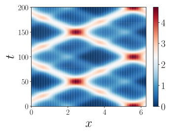
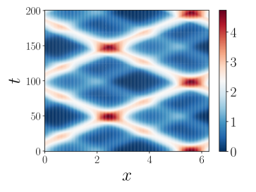
     G=0𝐺0{G=0}                                                G=βux4/4𝐺𝛽superscriptsubscript𝑢𝑥44{G=\beta u_{x}^{4}/4}

Refer to caption Refer to caption

Refer to caption Refer to caption

Refer to caption Refer to caption

Figure 1: Sample solutions of the nonlinear wave equation (80) with initial conditions u(x,0)=esin(2x)(1+cos(x))𝑢𝑥0superscript𝑒2𝑥1𝑥u(x,0)=e^{-\sin(2x)}(1+\cos(x)) (first row), u(x,0)=esin(2x)(1+cos(5x))𝑢𝑥0superscript𝑒2𝑥15𝑥u(x,0)=e^{-\sin(2x)}(1+\cos(5x))(second row), and u(x,0)=esin(2x)(1+cos(9x))𝑢𝑥0superscript𝑒2𝑥19𝑥u(x,0)=e^{-\sin(2x)}(1+\cos(9x)) (third row). We set the group velocity α𝛼\alpha to (2π/100)2superscript2𝜋1002(2\pi/100)^{2} and consider different nonlinear interaction terms: G=0𝐺0G=0 (first column – linear waves), G=βux4/4𝐺𝛽superscriptsubscript𝑢𝑥44G=\beta u_{x}^{4}/4 with β=(2π/100)4𝛽superscript2𝜋1004\beta=(2\pi/100)^{4} (second column – nonlinear waves). It is seen that as the initial condition becomes rougher, the nonlinear effects become more important.

4.1 Linear waves

Setting the interaction term G(p,ux,u)𝐺𝑝subscript𝑢𝑥𝑢G(p,u_{x},u) in (78) and (80) equal to zero yields the well-known linear wave equation

utt=αuxx.subscript𝑢𝑡𝑡𝛼subscript𝑢𝑥𝑥\displaystyle u_{tt}=\alpha u_{xx}. (82)

We discretize (82) in space using second-order finite differences on the (periodic) grid xj=2πj/Nsubscript𝑥𝑗2𝜋𝑗𝑁x_{j}=2\pi j/N (j=0,,N𝑗0𝑁j=0,\dots,N). This yields the following linear dynamical system

dujdt=pj,dpjdt=αh2(uj+12uj+uj1),formulae-sequence𝑑subscript𝑢𝑗𝑑𝑡subscript𝑝𝑗𝑑subscript𝑝𝑗𝑑𝑡𝛼superscript2subscript𝑢𝑗12subscript𝑢𝑗subscript𝑢𝑗1\frac{du_{j}}{dt}=p_{j},\qquad\frac{dp_{j}}{dt}=\frac{\alpha}{h^{2}}(u_{j+1}-2u_{j}+u_{j-1}), (83)

where uj(t)=u(xj,t)subscript𝑢𝑗𝑡𝑢subscript𝑥𝑗𝑡u_{j}(t)=u(x_{j},t), pj(t)=p(xj,t)subscript𝑝𝑗𝑡𝑝subscript𝑥𝑗𝑡p_{j}(t)=p(x_{j},t), and h=2π/N2𝜋𝑁h=2\pi/N is the mesh size. The Hamilton’s function corresponding to the finite-difference scheme (83) is obtained by discretizing the integral (78), e.g., with the rectangle rule. This yields

1(𝒑,𝒖)=j=0N1h2pj2+α1h2j=0N1(uj+1uj)2,subscript1𝒑𝒖superscriptsubscript𝑗0𝑁12superscriptsubscript𝑝𝑗2subscript𝛼12superscriptsubscript𝑗0𝑁1superscriptsubscript𝑢𝑗1subscript𝑢𝑗2\displaystyle\mathcal{H}_{1}(\bm{p},\bm{u})=\sum_{j=0}^{N-1}\frac{h}{2}p_{j}^{2}+\frac{\alpha_{1}h}{2}\sum_{j=0}^{N-1}(u_{j+1}-u_{j})^{2}, (84)

where we defined α1=α/h2subscript𝛼1𝛼superscript2\alpha_{1}=\alpha/h^{2}. The corresponding finite-dimensional Gibbs distribution can be written as

ρeq(𝒑,𝒖)=1Z1(α1,γ)exp{γ(j=0N112pj2+α12j=0N1(uj+1uj)2)},subscript𝜌𝑒𝑞𝒑𝒖1subscript𝑍1subscript𝛼1𝛾𝛾superscriptsubscript𝑗0𝑁112superscriptsubscript𝑝𝑗2subscript𝛼12superscriptsubscript𝑗0𝑁1superscriptsubscript𝑢𝑗1subscript𝑢𝑗2\displaystyle\rho_{eq}(\bm{p},\bm{u})=\frac{1}{Z_{1}(\alpha_{1},\gamma)}\exp\left\{-\gamma\left(\sum_{j=0}^{N-1}\frac{1}{2}p_{j}^{2}+\frac{\alpha_{1}}{2}\sum_{j=0}^{N-1}(u_{j+1}-u_{j})^{2}\right)\right\}, (85)

Z1(α1,γ)subscript𝑍1subscript𝛼1𝛾Z_{1}(\alpha_{1},\gamma) being the partition function (normalization constant). Note that we absorbed the scaling factor hh in the parameter γ>0𝛾0\gamma>0. It is straightforward to verify that the lattice Hamiltonian (84) is preserved if u0=uNsubscript𝑢0subscript𝑢𝑁u_{0}=u_{N} and p0=pNsubscript𝑝0subscript𝑝𝑁p_{0}=p_{N} (periodic boundary conditions). This implies that the PDF (85) is invariant under the flow generated by the linear ODE (83). Note that the lattice Hamiltonian (84) coincides with the Hamiltonian of a one-dimensional chain of harmonic oscillators with uniform mass m=1𝑚1m=1 and spring constants k=α1𝑘subscript𝛼1k=\alpha_{1}. We set N=100𝑁100N=100 and α=(2π/100)2𝛼superscript2𝜋1002\alpha=(2\pi/100)^{2} in equation (83). In this way, the system (83) is 200200200-dimensional and the modeling parameter α1subscript𝛼1\alpha_{1} in (84)-(85) is equal to 111.

     G=0𝐺0{G=0}                                                   G=βux4/4𝐺𝛽superscriptsubscript𝑢𝑥44{G=\beta u_{x}^{4}/4}

Refer to caption Refer to caption

Refer to caption Refer to caption

Refer to caption Refer to caption

Figure 2: Snapshots of the solution shown in Figure 1.

MZ memory kernel and auto-correlation functions

The Hamiltonian system (83) with periodic boundary conditions has many symmetries. In particular, the statistical properties of wave displacement u(x,t)𝑢𝑥𝑡u(x,t) at any point xjsubscript𝑥𝑗x_{j} are the same, if the initial state is distributed according to (85). In addition, the PDF of the wave momentum999Note that for linear waves the wave momentum p(x,t)𝑝𝑥𝑡p(x,t) is equal to u(x,t)/t𝑢𝑥𝑡𝑡\partial u(x,t)/\partial t (see Eq. (79)). p(xj,t)𝑝subscript𝑥𝑗𝑡p(x_{j},t) and the wave displacement r(xj,t)=u(xj+1,t)u(xj,t)𝑟subscript𝑥𝑗𝑡𝑢subscript𝑥𝑗1𝑡𝑢subscript𝑥𝑗𝑡r(x_{j},t)=u(x_{j+1},t)-u(x_{j},t) are both Gaussian (see Eq. (85)). Suppose we are interested in the temporal auto-correlation function of the wave momentum p(xj,t)=pj𝑝subscript𝑥𝑗𝑡subscript𝑝𝑗p(x_{j},t)=p_{j}, at an arbitrary location xjsubscript𝑥𝑗x_{j}, i.e.,

Cpj(t)=pj(t),pj(0)eq,subscript𝐶subscript𝑝𝑗𝑡subscriptsubscript𝑝𝑗𝑡subscript𝑝𝑗0𝑒𝑞C_{p_{j}}(t)=\langle p_{j}(t),p_{j}(0)\rangle_{eq}, (86)

where ,eq\langle,\rangle_{eq} is an integral over the equilibrium distribution (85). Such correlation function admits the analytical expression (see [20])

Cpj(t)=J0(2t),γ>0,formulae-sequencesubscript𝐶subscript𝑝𝑗𝑡subscript𝐽02𝑡for-all𝛾0\displaystyle C_{p_{j}}(t)=J_{0}(2t),\qquad\forall\gamma>0, (87)

where J0subscript𝐽0J_{0} is the zero-order Bessel function of the first kind. With Cpj(t)subscript𝐶subscript𝑝𝑗𝑡C_{p_{j}}(t) available, we can solve the MZ equation

ddtCpj(t)=0tK(ts)Cpj(s)𝑑s𝑑𝑑𝑡subscript𝐶subscript𝑝𝑗𝑡superscriptsubscript0𝑡𝐾𝑡𝑠subscript𝐶subscript𝑝𝑗𝑠differential-d𝑠\displaystyle\frac{d}{dt}C_{p_{j}}(t)=\int_{0}^{t}K(t-s)C_{p_{j}}(s)ds (88)

for the memory kernel K(t)𝐾𝑡K(t) by using Laplace transforms. This yields the exact MZ kernel

K(t)=J1(2t)t,γ>0,formulae-sequence𝐾𝑡subscript𝐽12𝑡𝑡for-all𝛾0K(t)=\frac{J_{1}(2t)}{t},\qquad\forall\gamma>0, (89)

where J1subscript𝐽1J_{1} is the first-order Bessel function of the first kind. In Figure 3, we compare the exact memory kernel (89) and the correlation function (88) with the results we obtained using the iterative algorithm discussed in Section 2.5. Note that the system (83) is linear. Therefore, we can use the formula (42) to compute the coefficients {γ1,,γn+2}subscript𝛾1subscript𝛾𝑛2\{\gamma_{1},\dots,\gamma_{n+2}\}. With such coefficients available, we then compute {μ1,,μn+2}subscript𝜇1subscript𝜇𝑛2\{\mu_{1},\dots,\mu_{n+2}\} using the recurrence relation (27), and the MZ memory kernel (22). In Figure (3) we demonstrate that the MZ-Faber expansion rapidly converges to the exact auto-correlation function (86) of the wave momentum as we increase the Faber expansion order n𝑛n. This is not surprising since the linear wave equation is a well-known integrable system for which convergence of the MZ-Faber series can be rigorously established (§5 in [68]).
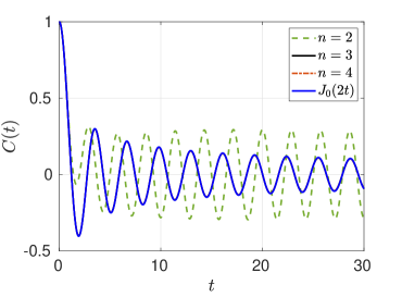
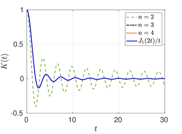
Refer to caption Refer to caption

Figure 3: Linear wave equation (82). Temporal auto-correlation function of the wave momentum p(xj,t)=u(xj,t)/t𝑝subscript𝑥𝑗𝑡𝑢subscript𝑥𝑗𝑡𝑡p(x_{j},t)={\partial u(x_{j},t)}/\partial t (Eq. (86), any location xjsubscript𝑥𝑗x_{j}) and MZ memory kernel K(t)𝐾𝑡K(t). We compare the the analytical results (87) and (89), with results we obtained by using the recursive algorithm we presented in Section 2.3 for different Faber polynomial orders n𝑛n. It is seen that the MZ-Faber expansion rapidly converges to the exact MZ-kernel and auto-correlation function we increase the polynomial order.

Reduced-order stochastic modeling

Suppose we are interested in building a consistent reduced-order stochastic model for the wave momentum p(xj,t)=u(xj,t)/t𝑝subscript𝑥𝑗𝑡𝑢subscript𝑥𝑗𝑡𝑡p(x_{j},t)=\partial u(x_{j},t)/\partial t at statistical equilibrium. To this end, we employ the spectral expansion technique we discussed in Section 3. The auto-correlation function of the process p(t)=p(xj,t)𝑝𝑡𝑝subscript𝑥𝑗𝑡p(t)=p(x_{j},t) (at any location xjsubscript𝑥𝑗x_{j}), i.e., (86), is obtained by solving the MZ equation (88) with the kernel computed using the combinatorial algorithm described in Section 2.5. Following the stochastic modeling paradigm we developed in Section 3, we expand p(t)𝑝𝑡p(t) as

p(t)k=1Kλkξk(ω)ek(t),similar-to-or-equals𝑝𝑡superscriptsubscript𝑘1𝐾subscript𝜆𝑘subscript𝜉𝑘𝜔subscript𝑒𝑘𝑡p(t)\simeq\sum_{k=1}^{K}\sqrt{\lambda_{k}}\xi_{k}(\omega)e_{k}(t), (90)

where (λk,ek(t))subscript𝜆𝑘subscript𝑒𝑘𝑡(\lambda_{k},e_{k}(t)) are eigenvalues and eigenfunctions of (86). By enforcing consistency of (90) with the equilibrium distribution (85) at each fixed time we obtain that the random variables p(tj)𝑝subscript𝑡𝑗p(t_{j}) are normally distributed with zero mean and variance 1/γ1𝛾1/\gamma, for all tj[0,10]subscript𝑡𝑗010t_{j}\in[0,10]. In other words p(t)𝑝𝑡p(t) is a centered, stationary Gaussian random process with correlation function (86). In Figure 4, we plot the auto-correlation functions

Cp(t)=pj(t),pj(0)eq,Cp2(t)=pj2(t),pj2(0)eq,Cp4(t)=pj4(t),pj4(0)eq,formulae-sequencesubscript𝐶𝑝𝑡subscriptsubscript𝑝𝑗𝑡subscript𝑝𝑗0𝑒𝑞formulae-sequencesuperscriptsubscript𝐶𝑝2𝑡subscriptsubscriptsuperscript𝑝2𝑗𝑡subscriptsuperscript𝑝2𝑗0𝑒𝑞superscriptsubscript𝐶𝑝4𝑡subscriptsubscriptsuperscript𝑝4𝑗𝑡subscriptsuperscript𝑝4𝑗0𝑒𝑞\displaystyle C_{p}(t)=\langle p_{j}(t),p_{j}(0)\rangle_{eq},\qquad C_{p}^{2}(t)=\langle p^{2}_{j}(t),p^{2}_{j}(0)\rangle_{eq},\qquad C_{p}^{4}(t)=\langle p^{4}_{j}(t),p^{4}_{j}(0)\rangle_{eq}, (91)

we obtained with an MZ-Faber expansion of degree n=6𝑛6n=6. Convergence of KL expansions representing high-order correlation functions such as (91) is established in Appendix.
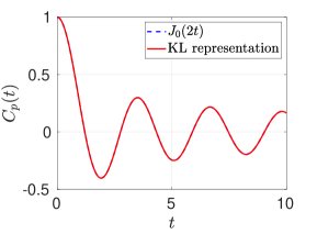
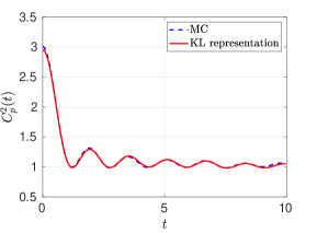
Refer to caption
Refer to caption
Refer to caption
Figure 4: Linear wave equation (82). Temporal auto-correlation functions (91) of the wave momentum. The MZ kernel here is approximated with a Faber polynomial series of degree n=10𝑛10n=10.

4.2 Nonlinear waves

Here we study the nonlinear wave equation (80) with interaction term G(p,ux,u)=βux4/4𝐺𝑝subscript𝑢𝑥𝑢𝛽superscriptsubscript𝑢𝑥44G(p,u_{x},u)=\beta u_{x}^{4}/4, i.e.,

utt=αuxx+3βux2uxx,α,β>0.formulae-sequencesubscript𝑢𝑡𝑡𝛼subscript𝑢𝑥𝑥3𝛽superscriptsubscript𝑢𝑥2subscript𝑢𝑥𝑥𝛼𝛽0\displaystyle u_{tt}=\alpha u_{xx}+3\beta u_{x}^{2}u_{xx},\qquad\alpha,\beta>0. (92)

In Figure 1 and Figure 2 we plot sample solutions of (92) corresponding to different initial conditions. It is clearly seen that the nonlinearity ux2uxxsuperscriptsubscript𝑢𝑥2subscript𝑢𝑥𝑥u_{x}^{2}u_{xx} breaks the periodicity of traveling wave. This effect is more pronounced if the initial condition is rougher in x𝑥x, as ux2subscriptsuperscript𝑢2𝑥u^{2}_{x} and uxxsubscript𝑢𝑥𝑥u_{xx} are larger in this case, thereby increasing magnitude of the nonlinear term in (92). As before, we discretize (92) and the Hamiltonian (78) with finite differences on a periodic spatial grid (N𝑁N points in [0,2π]02𝜋[0,2\pi]). This yields

2(𝒑,𝒖)=j=0N1hpj22+j=0N1hα12(uj+1uj)2+j=0N1hβ14(uj+1uj)4,subscript2𝒑𝒖superscriptsubscript𝑗0𝑁1superscriptsubscript𝑝𝑗22superscriptsubscript𝑗0𝑁1subscript𝛼12superscriptsubscript𝑢𝑗1subscript𝑢𝑗2superscriptsubscript𝑗0𝑁1subscript𝛽14superscriptsubscript𝑢𝑗1subscript𝑢𝑗4\displaystyle\mathcal{H}_{2}(\bm{p},\bm{u})=\sum_{j=0}^{N-1}\frac{hp_{j}^{2}}{2}+\sum_{j=0}^{N-1}\frac{h\alpha_{1}}{2}(u_{j+1}-u_{j})^{2}+\sum_{j=0}^{N-1}\frac{h\beta_{1}}{4}(u_{j+1}-u_{j})^{4}, (93)

where uj(t)=u(xj,t)subscript𝑢𝑗𝑡𝑢subscript𝑥𝑗𝑡u_{j}(t)=u(x_{j},t) and pj(t)=u(xj,t)/tsubscript𝑝𝑗𝑡𝑢subscript𝑥𝑗𝑡𝑡p_{j}(t)=\partial u(x_{j},t)/\partial t represent the wave amplitude and momentum at location xj=hjsubscript𝑥𝑗𝑗x_{j}=hj (j=0,,N𝑗0𝑁j=0,\dots,N, h=2π/N2𝜋𝑁h=2\pi/N), α1=α/h2subscript𝛼1𝛼superscript2\alpha_{1}=\alpha/h^{2} and β1=β/h4subscript𝛽1𝛽superscript4\beta_{1}=\beta/h^{4}. The discretized equilibrium distribution (81) then becomes

ρeq(𝒑,𝒖)=1Z2(α1,β1,γ)exp{γ(j=0N1pj22+j=0N1α12(uj+1uj)2+j=0N1β14(uj+1uj)4)}.subscript𝜌𝑒𝑞𝒑𝒖1subscript𝑍2subscript𝛼1subscript𝛽1𝛾𝛾superscriptsubscript𝑗0𝑁1superscriptsubscript𝑝𝑗22superscriptsubscript𝑗0𝑁1subscript𝛼12superscriptsubscript𝑢𝑗1subscript𝑢𝑗2superscriptsubscript𝑗0𝑁1subscript𝛽14superscriptsubscript𝑢𝑗1subscript𝑢𝑗4\displaystyle\rho_{eq}(\bm{p},\bm{u})=\frac{1}{Z_{2}(\alpha_{1},\beta_{1},\gamma)}\exp\left\{-\gamma\left(\sum_{j=0}^{N-1}\frac{p_{j}^{2}}{2}+\sum_{j=0}^{N-1}\frac{\alpha_{1}}{2}(u_{j+1}-u_{j})^{2}+\sum_{j=0}^{N-1}\frac{\beta_{1}}{4}(u_{j+1}-u_{j})^{4}\right)\right\}. (94)

As before, we absorbed the factor hh into the parameter γ𝛾\gamma. Note that the lattice Hamiltonian (93) coincides with the Hamiltonian of the Fermi-Pasta-Ulam β𝛽\beta-model (54), with mj=1subscript𝑚𝑗1m_{j}=1. We emphasize that if a different scheme is used to discretize the wave equation (92), then the lattice Hamiltonian (93) may not be a conserved quantity.

MZ memory term and auto-correlation functions

We choose the wave momentum pj(t)subscript𝑝𝑗𝑡p_{j}(t) and the wave displacement rj(t)=uj+1(t)uj(t)subscript𝑟𝑗𝑡subscript𝑢𝑗1𝑡subscript𝑢𝑗𝑡r_{j}(t)=u_{j+1}(t)-u_{j}(t) as quantities of interest. Moreover, we set N=100𝑁100N=100 and α=(2π/100)2𝛼superscript2𝜋1002\alpha=(2\pi/100)^{2}. To study the effects of the nonlinear interaction term, we consider different values of β=β1α2𝛽subscript𝛽1superscript𝛼2\beta=\beta_{1}\alpha^{2}, with β1subscript𝛽1\beta_{1} ranging from 0.010.010.01 to 111. This corresponds to the FPU models with mild and strong nonlinearities, respectively. Based on the structure of the Hamiltonian (93) and the equilibrium distribution (94), we expect that the dynamics of pj(t)subscript𝑝𝑗𝑡p_{j}(t) and rj(t)subscript𝑟𝑗𝑡r_{j}(t) will be different for different parameters β𝛽\beta. To calculate the temporal auto-correlation function of pj(t)subscript𝑝𝑗𝑡p_{j}(t) and rj(t)subscript𝑟𝑗𝑡r_{j}(t) at an arbitrary spatial point xjsubscript𝑥𝑗x_{j}, we solve the corresponding MZ equations. Such equations are of the form (88), where the memory kernel K(ts)𝐾𝑡𝑠K(t-s) is computed from first-principles (i.e., from the microscopic equations of motion) using the algorithm we presented in Section 2.5. In Figure 5, we compare the temporal auto-correlation function we obtained for the wave displacement rj(t)subscript𝑟𝑗𝑡r_{j}(t) with results of Markov-Chain-Monte-Carlo (MCMC) (106superscript10610^{6} sample paths) for FPU systems with mild nonlinearities (β1=0.01subscript𝛽10.01\beta_{1}=0.01 and β1=0.1subscript𝛽10.1\beta_{1}=0.1 ) at different temperatures (γ=1𝛾1\gamma=1 and γ=40𝛾40\gamma=40). It is seen that the MZ-Faber approximation of the MZ memory kernel yields relatively accurate results for FPU systems with mild nonlinearties at both low (γ=40𝛾40\gamma=40) and high temperature (γ=1𝛾1\gamma=1) as we increase the polynomial order n𝑛n.

     β1=0.01subscript𝛽10.01{\beta_{1}=0.01}                                                     β1=0.1subscript𝛽10.1{\beta_{1}=0.1}

Refer to caption Refer to caption

Refer to caption Refer to caption

Figure 5: Nonlinear wave equation (92). Temporal auto-correlation function of the wave displacement rj(t)subscript𝑟𝑗𝑡r_{j}(t) for different values of the nonlinear parameter β1subscript𝛽1\beta_{1}. We compare results we obtained by calculating the MZ memory from first principles using n𝑛n-th order Faber polynomials (Section 2.4) with results from Markov-Chain-Monte-Carlo (106superscript10610^{6} sample paths). The thermodynamic parameter γ𝛾\gamma is set to 1 (high-temperature) in the first row and to 40 (low-temperature) in the second row.

Reduced-order stochastic modeling

We employ the spectral approach of Section 3 to build stochastic low-dimensional models of the wave momentum pj(t)subscript𝑝𝑗𝑡p_{j}(t) and wave displacement rj(t)=uj+1(t)uj(t)subscript𝑟𝑗𝑡subscript𝑢𝑗1𝑡subscript𝑢𝑗𝑡r_{j}(t)=u_{j+1}(t)-u_{j}(t) at statistical equilibrium. Since we assumed that we are at statistical equilibrium, the statistical properties of the random processes representing pj(t)subscript𝑝𝑗𝑡p_{j}(t) and rj(t)subscript𝑟𝑗𝑡r_{j}(t) are time-independent. For instance, by integrating (94) we obtain the following expression for the one-time PDF of rj(t)subscript𝑟𝑗𝑡r_{j}(t)

rj(t)eγ(12α1r2+14β1r4)t[0,T],j=0,,N1.formulae-sequencesimilar-tosubscript𝑟𝑗𝑡superscript𝑒𝛾12subscript𝛼1superscript𝑟214subscript𝛽1superscript𝑟4formulae-sequencefor-all𝑡0𝑇for-all𝑗0𝑁1r_{j}(t)\sim e^{-\gamma(\frac{1}{2}\alpha_{1}r^{2}+\frac{1}{4}\beta_{1}r^{4})}\qquad\forall t\in[0,T],\quad\forall j=0,\dots,N-1. (95)

Clearly, rj(t)subscript𝑟𝑗𝑡r_{j}(t) is a stationary non-Gaussian process. To sample the KL expansion of rj(t)subscript𝑟𝑗𝑡r_{j}(t) in a way that is consistent with the PDF (95) we used the algorithm discussed in [49, 50]. For the FPU system with α1=β1=1subscript𝛼1subscript𝛽11\alpha_{1}=\beta_{1}=1, it is straightforward to show that for all m𝑚m\in\mathbb{N}

𝔼{rj2m(t)}=+r2meγ(12r214r4)𝑑r+eγ(12r214r4)𝑑r=2γ14m2Γ(12+m)U(14+m2,12,γ4)eγ/8K1/4(γ8),𝔼superscriptsubscript𝑟𝑗2𝑚𝑡superscriptsubscriptsuperscript𝑟2𝑚superscript𝑒𝛾12superscript𝑟214superscript𝑟4differential-d𝑟superscriptsubscriptsuperscript𝑒𝛾12superscript𝑟214superscript𝑟4differential-d𝑟2superscript𝛾14𝑚2Γ12𝑚𝑈14𝑚212𝛾4superscript𝑒𝛾8subscript𝐾14𝛾8\displaystyle\mathbb{E}\{r_{j}^{2m}(t)\}=\frac{\displaystyle\int_{-\infty}^{+\infty}r^{2m}e^{-\gamma(\frac{1}{2}r^{2}-\frac{1}{4}r^{4})}dr}{\displaystyle\int_{-\infty}^{+\infty}e^{-\gamma(\frac{1}{2}r^{2}-\frac{1}{4}r^{4})}dr}=\frac{\sqrt{2}\gamma^{-\frac{1}{4}-\frac{m}{2}}\Gamma\left(\frac{1}{2}+m\right)U\left(\frac{1}{4}+\frac{m}{2},\frac{1}{2},\frac{\gamma}{4}\right)}{e^{\gamma/8}K_{1/4}\left(\frac{\gamma}{8}\right)},

where Γ(x)Γ𝑥\Gamma(x) is the Gamma function, Kn(z)subscript𝐾𝑛𝑧K_{n}(z) is the modified Bessel function of the second kind and U(x,y,z)𝑈𝑥𝑦𝑧U(x,y,z) is Tricomi’s confluent hypergeometric function. Therefore, for all positive γ𝛾\gamma and finite m𝑚m we have that 𝔼{rj2m(t)}<𝔼superscriptsubscript𝑟𝑗2𝑚𝑡\mathbb{E}\{r_{j}^{2m}(t)\}<\infty, i.e., rj(t)subscript𝑟𝑗𝑡r_{j}(t) is L2msuperscript𝐿2𝑚L^{2m} process. This condition guarantees convergence of the KL expansion to temporal correlation functions of order greater than two (see Appendix A). In Figure 6 we plot the temporal auto-correlation function of various polynomial observables of the nonlinear wave momentum and displacement at an arbitrary spatial point xjsubscript𝑥𝑗x_{j}. We compare results we obtained from Markov Chain Monte Carlo simulation (dashed line), with the MZ-KL expansion method based the first-principle memory calculation (continuous line). We also provide results we obtained by using KL expansions with covariance kernel estimated from data (dotted line).
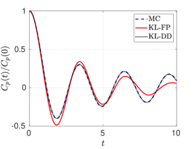
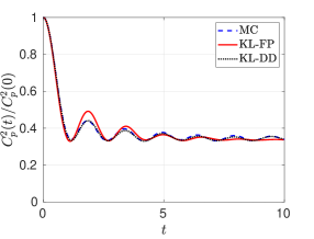
Refer to caption Refer to caption Refer to caption

Refer to caption Refer to caption Refer to caption

Figure 6: Nonlinear wave equaton (92). Temporal auto-correlation function of polynomial observables pjm(t)superscriptsubscript𝑝𝑗𝑚𝑡p_{j}^{m}(t) (first row) rjm(t)superscriptsubscript𝑟𝑗𝑚𝑡r_{j}^{m}(t) (second row) with m=1,2,4𝑚124m=1,2,4. We compare results from Markov-Chain-Monte-Carlo simulation (MC), KL expansion based on the first-principle MZ memory kernel calculation (88) (KL-FP), and KL expansion based on a data-driven estimate of the temporal auto-correlation function (KL-DD). The parameter γ𝛾\gamma appearing in (94) is set to 404040, while α1=β1=1subscript𝛼1subscript𝛽11\alpha_{1}=\beta_{1}=1.

5 Summary

We developed a new method to approximate the Mori-Zwanzig (MZ) memory integral in generalized Langevin equations (GLEs) describing the evolution of smooth observables in high-dimensional nonlinear systems with local interactions. The new method is based on Faber operator series expansions [68], and a formally exact combinatorial algorithm that allows us to compute the expansion coefficients of the MZ memory from first principles, i.e., based on the microscopic equations of motion. We also developed a new stochastic modeling technique that employs Karhunen-Loève expansions to represent the MZ fluctuation term (random noise) for systems in statistical equilibrium. We demonstrated the MZ memory calculation method and the MZ-KL stochastic modeling technique in applications to random wave propagation and prototype problems in classical statistical mechanics such as the Fermi-Pasta-Ulam β𝛽\beta-model. We found that the proposed algorithms can accurately capture relaxation to statistical equilibrium in systems with mild nonlinearities, and in strongly nonlinear systems at high-temperature. At low temperature the Faber expansion of the MZ memory kernel is granted to converge only on a time interval that depends on the system and on the observable. In particular, Corollary 3.4.3 in [67] establishes short-time convergence of the MZ-Faber memory approximation for a broad class of nonlinear systems of the form (1). This implies that the MZ-Faber cumulant expansion can exhibit short-time convergence, meaning that it produces first-principle results that are accurate only for relatively short integration times.

We conclude by emphasizing that the mathematical techniques we presented can be readily applied to more general systems with local interactions such as particle systems modeling the microscopic dynamics of solids and liquids [66, 37, 38]. This opens the possibility to build new approximation schemes for MZ equations and derive new types of coarse-grained models where the MZ memory is constructed from first-principles and the fluctuation term is modeled stochastically.

Acknowledgements This research was supported by the Air Force Office of Scientific Research (AFOSR) grant FA9550-16-586-1-0092.

Appendix A Auto-correlation function of polynomial observables

In this Appendix we prove that the temporal auto-correlation function of phase space functions of the form un(t)=un(𝒙(t,𝒙0))superscript𝑢𝑛𝑡superscript𝑢𝑛𝒙𝑡subscript𝒙0u^{n}(t)=u^{n}(\bm{x}(t,\bm{x}_{0})), i.e.,

un(0),un(t)ρnsubscriptsuperscript𝑢𝑛0superscript𝑢𝑛𝑡𝜌𝑛\langle u^{n}(0),u^{n}(t)\rangle_{\rho}\qquad n\in\mathbb{N} (96)

can be represented by replacing u(t)𝑢𝑡u(t) with the KL expansion (66), and then sending K𝐾K to infinity. This result allows us to compute the auto-correlation function of un(t)superscript𝑢𝑛𝑡u^{n}(t) based on the KL expansions of u(t)𝑢𝑡u(t).

Theorem A.1 Consider a zero-mean stationary stochastic process u(t)𝑢𝑡u(t), t[0,T]𝑡0𝑇t\in[0,T], and assume that it has finite joint moments up to any desired order. Let

uK(t)=k=1Kλkξkek(t),subscript𝑢𝐾𝑡superscriptsubscript𝑘1𝐾subscript𝜆𝑘subscript𝜉𝑘subscript𝑒𝑘𝑡u_{K}(t)=\sum_{k=1}^{K}\sqrt{\lambda_{k}}\xi_{k}e_{k}(t),\qquad (97)

be the truncated Karhunen-Loève expansion of u(t)𝑢𝑡u(t). Then

limK|un(0),un(t)ρuKn(0),uKn(t)ρ|n,subscript𝐾subscriptsuperscript𝑢𝑛0superscript𝑢𝑛𝑡𝜌subscriptsuperscriptsubscript𝑢𝐾𝑛0superscriptsubscript𝑢𝐾𝑛𝑡𝜌for-all𝑛\lim_{K\rightarrow\infty}\left|\langle u^{n}(0),u^{n}(t)\rangle_{\rho}-\langle u_{K}^{n}(0),u_{K}^{n}(t)\rangle_{\rho}\right|\qquad\forall n\in\mathbb{N}, (98)

i.e., uKn(0),uKn(t)ρsubscriptsuperscriptsubscript𝑢𝐾𝑛0superscriptsubscript𝑢𝐾𝑛𝑡𝜌\langle u_{K}^{n}(0),u_{K}^{n}(t)\rangle_{\rho} converges uniformly to un(0),un(t)ρsubscriptsuperscript𝑢𝑛0superscript𝑢𝑛𝑡𝜌\langle u^{n}(0),u^{n}(t)\rangle_{\rho} as K𝐾K\rightarrow\infty.

Proof.

Let us define

δK(t)subscript𝛿𝐾𝑡\displaystyle\delta_{K}(t) =|uKn(t),uKn(0)un(t),u(0)|absentsuperscriptsubscript𝑢𝐾𝑛𝑡superscriptsubscript𝑢𝐾𝑛0superscript𝑢𝑛𝑡𝑢0\displaystyle=\left|\langle u_{K}^{n}(t),u_{K}^{n}(0)\rangle-\langle u^{n}(t),u(0)\rangle\right|
=|uKn(t),uKn(0)un(t),uKn(0)+un(t),uKn(0)un(t),un(0)|absentsuperscriptsubscript𝑢𝐾𝑛𝑡superscriptsubscript𝑢𝐾𝑛0superscript𝑢𝑛𝑡subscriptsuperscript𝑢𝑛𝐾0superscript𝑢𝑛𝑡subscriptsuperscript𝑢𝑛𝐾0superscript𝑢𝑛𝑡superscript𝑢𝑛0\displaystyle=|\langle u_{K}^{n}(t),u_{K}^{n}(0)\rangle-\langle u^{n}(t),u^{n}_{K}(0)\rangle+\langle u^{n}(t),u^{n}_{K}(0)\rangle-\langle u^{n}(t),u^{n}(0)\rangle|
=|uKn(t)un(t),uKn(0)+un(t),uKn(0)un(0)|absentsuperscriptsubscript𝑢𝐾𝑛𝑡superscript𝑢𝑛𝑡superscriptsubscript𝑢𝐾𝑛0superscript𝑢𝑛𝑡subscriptsuperscript𝑢𝑛𝐾0superscript𝑢𝑛0\displaystyle=|\langle u_{K}^{n}(t)-u^{n}(t),u_{K}^{n}(0)\rangle+\langle u^{n}(t),u^{n}_{K}(0)-u^{n}(0)\rangle|
|uKn(t)un(t),uKn(0)|+|un(t),uKn(0)un(0)|absentsuperscriptsubscript𝑢𝐾𝑛𝑡superscript𝑢𝑛𝑡superscriptsubscript𝑢𝐾𝑛0superscript𝑢𝑛𝑡subscriptsuperscript𝑢𝑛𝐾0superscript𝑢𝑛0\displaystyle\leq|\langle u_{K}^{n}(t)-u^{n}(t),u_{K}^{n}(0)\rangle|+|\langle u^{n}(t),u^{n}_{K}(0)-u^{n}(0)\rangle| (99)

The first term at the right hand side is of the form

anbn=(ab)i=0n1aibn1i.superscript𝑎𝑛superscript𝑏𝑛𝑎𝑏superscriptsubscript𝑖0𝑛1superscript𝑎𝑖superscript𝑏𝑛1𝑖\displaystyle a^{n}-b^{n}=(a-b)\sum_{i=0}^{n-1}a^{i}b^{n-1-i}.

By using the Cauchy-Schwarz inequality, we obtain

|uKn(t)un(t),uKn(0)|=superscriptsubscript𝑢𝐾𝑛𝑡superscript𝑢𝑛𝑡superscriptsubscript𝑢𝐾𝑛0absent\displaystyle|\langle u_{K}^{n}(t)-u^{n}(t),u_{K}^{n}(0)\rangle|= |(uK(t)u(t))i=0n1uKi(t)un1i(t),uKn(0)|subscript𝑢𝐾𝑡𝑢𝑡superscriptsubscript𝑖0𝑛1superscriptsubscript𝑢𝐾𝑖𝑡superscript𝑢𝑛1𝑖𝑡superscriptsubscript𝑢𝐾𝑛0\displaystyle\left|\langle(u_{K}(t)-u(t))\sum_{i=0}^{n-1}u_{K}^{i}(t)u^{n-1-i}(t),u_{K}^{n}(0)\rangle\right|
=\displaystyle= |uK(t)u(t),uKn(0)i=0n1uKi(t)un1i(t)|subscript𝑢𝐾𝑡𝑢𝑡superscriptsubscript𝑢𝐾𝑛0superscriptsubscript𝑖0𝑛1superscriptsubscript𝑢𝐾𝑖𝑡superscript𝑢𝑛1𝑖𝑡\displaystyle\left|\langle u_{K}(t)-u(t),u_{K}^{n}(0)\sum_{i=0}^{n-1}u_{K}^{i}(t)u^{n-1-i}(t)\rangle\right|
\displaystyle\leq ϵK(t)uKn(0)i=1n1uKi(t)un1i(t)L2,subscriptitalic-ϵ𝐾𝑡subscriptnormsuperscriptsubscript𝑢𝐾𝑛0superscriptsubscript𝑖1𝑛1superscriptsubscript𝑢𝐾𝑖𝑡superscript𝑢𝑛1𝑖𝑡superscript𝐿2\displaystyle\epsilon_{K}(t)\left\|u_{K}^{n}(0)\sum_{i=1}^{n-1}u_{K}^{i}(t)u^{n-1-i}(t)\right\|_{L^{2}},

where we defined ϵK(t)=uK(t)u(t)L2subscriptitalic-ϵ𝐾𝑡subscriptnormsubscript𝑢𝐾𝑡𝑢𝑡superscript𝐿2\epsilon_{K}(t)=\|u_{K}(t)-u(t)\|_{L^{2}}. It is well-known that ϵK(t)0subscriptitalic-ϵ𝐾𝑡0\epsilon_{K}(t)\rightarrow 0 as K𝐾K\rightarrow\infty (see, e.g., [41]). By using the generalized Hölder’s inequality fgLpfLqgLqsubscriptnorm𝑓𝑔superscript𝐿𝑝subscriptnorm𝑓superscript𝐿𝑞subscriptnorm𝑔superscript𝐿𝑞\|fg\|_{L^{p}}\leq\|f\|_{L^{q}}\|g\|_{L^{q}}, where 2p=q2𝑝𝑞2p=q and the Minkowski inequality, we obtain

|uKn(t)un(t),uKn(0)|superscriptsubscript𝑢𝐾𝑛𝑡superscript𝑢𝑛𝑡superscriptsubscript𝑢𝐾𝑛0\displaystyle|\langle u_{K}^{n}(t)-u^{n}(t),u_{K}^{n}(0)\rangle| ϵK(t)uKn(0)L4i=1n1uKi(t)uni1(t)L4absentsubscriptitalic-ϵ𝐾𝑡subscriptnormsuperscriptsubscript𝑢𝐾𝑛0superscript𝐿4superscriptsubscript𝑖1𝑛1subscriptnormsuperscriptsubscript𝑢𝐾𝑖𝑡superscript𝑢𝑛𝑖1𝑡superscript𝐿4\displaystyle\leq\epsilon_{K}(t)\|u_{K}^{n}(0)\|_{L^{4}}\sum_{i=1}^{n-1}\|u_{K}^{i}(t)u^{n-i-1}(t)\|_{L^{4}}
ϵK(t)uKn(0)L4i=1n1uKi(t)L8uni1(t)L8=C1ϵK(t),absentsubscriptitalic-ϵ𝐾𝑡subscriptnormsuperscriptsubscript𝑢𝐾𝑛0superscript𝐿4superscriptsubscript𝑖1𝑛1subscriptnormsuperscriptsubscript𝑢𝐾𝑖𝑡superscript𝐿8subscriptnormsuperscript𝑢𝑛𝑖1𝑡superscript𝐿8subscript𝐶1subscriptitalic-ϵ𝐾𝑡\displaystyle\leq\epsilon_{K}(t)\|u_{K}^{n}(0)\|_{L^{4}}\sum_{i=1}^{n-1}\|u_{K}^{i}(t)\|_{L^{8}}\|u^{n-i-1}(t)\|_{L^{8}}=C_{1}\epsilon_{K}(t), (100)

where

C1=uKn(0)L4i=1n1uKi(t)L8uni1(t)L8<.subscript𝐶1subscriptnormsuperscriptsubscript𝑢𝐾𝑛0superscript𝐿4superscriptsubscript𝑖1𝑛1subscriptnormsuperscriptsubscript𝑢𝐾𝑖𝑡superscript𝐿8subscriptnormsuperscript𝑢𝑛𝑖1𝑡superscript𝐿8C_{1}=\|u_{K}^{n}(0)\|_{L^{4}}\sum_{i=1}^{n-1}\|u_{K}^{i}(t)\|_{L^{8}}\|u^{n-i-1}(t)\|_{L^{8}}<\infty. (101)

Similarly, we have

|un(t),uKn(0)un(0)|ϵK(0)un(0)L4i=1n1uKi(0)L8uni1(0)L8=C2ϵK(0).superscript𝑢𝑛𝑡superscriptsubscript𝑢𝐾𝑛0superscript𝑢𝑛0subscriptitalic-ϵ𝐾0subscriptnormsuperscript𝑢𝑛0superscript𝐿4superscriptsubscript𝑖1𝑛1subscriptnormsuperscriptsubscript𝑢𝐾𝑖0superscript𝐿8subscriptnormsuperscript𝑢𝑛𝑖10superscript𝐿8subscript𝐶2subscriptitalic-ϵ𝐾0\displaystyle|\langle u^{n}(t),u_{K}^{n}(0)-u^{n}(0)\rangle|\leq\epsilon_{K}(0)\|u^{n}(0)\|_{L^{4}}\sum_{i=1}^{n-1}\|u_{K}^{i}(0)\|_{L^{8}}\|u^{n-i-1}(0)\|_{L^{8}}=C_{2}\epsilon_{K}(0). (102)

By combining (99), (A) and (102), we obtain

limK+δK(t)limK+C1ϵK(t)+C2ϵK(0)=0,subscript𝐾subscript𝛿𝐾𝑡subscript𝐾subscript𝐶1subscriptitalic-ϵ𝐾𝑡subscript𝐶2subscriptitalic-ϵ𝐾00\displaystyle\lim_{K\rightarrow+\infty}\delta_{K}(t)\leq\lim_{K\rightarrow+\infty}C_{1}\epsilon_{K}(t)+C_{2}\epsilon_{K}(0)=0,

which proves the theorem.

References

  • [1] G. Amati, H. Meyer, and T. Schilling. Memory effects in the Fermi–Pasta–Ulam model. J. Stat. Phys., 174(1):219–257, 2019.
  • [2] N. Aubry, R. Guyonnet, and R. Lima. Spatiotemporal analysis of complex signals: theory and applications. J. Stat. Phys., 64:683–739, 1991.
  • [3] N. Aubry and R. Lima. Spatiotemporal and statistical symmetries. J. Stat. Phys., 81(3/4):793–828, 1995.
  • [4] M. Berkowitz, J. D. Morgan, D. J. Kouri, and J. A. McCammon. Memory kernels from molecular dynamics. J. Chem. Phys, 75(5):2462–2463, 1981.
  • [5] B. J. Berne and G. D. Harp. On the calculation of time correlation functions. Adv. Chem. Phys., pages 63–227, 1970.
  • [6] F. F. Bouchet and M. Corvellec. Invariant measures of the 2D Euler and Vlasov equations. J. Stat. Mech.: Theory and Experiment, 2010(08):P08021, 2010.
  • [7] C. Brennan and D. Venturi. Data-driven closures for stochastic dynamical systems. J. Comp. Phys.,, 372:281–298, 2018.
  • [8] A. Chertock, D. Gottlieb, and A. Solomonoff. Modified optimal prediction and its application to a particle-method problem. J. Sci. Comp., 37(2):189–201, 2008.
  • [9] H. Cho, D. Venturi, and G. E. Karniadakis. Karhunen-Loev̀e expansion for multi-correlated stochastic processes. Prob. Eng. Mech., 34:157–167, 2013.
  • [10] H. Cho, D. Venturi, and G. E. Karniadakis. Statistical analysis and simulation of random shocks in Burgers equation. Proc. R. Soc. A, 2171(470):1–21, 2014.
  • [11] A. J. Chorin, O. H. Hald, and R. Kupferman. Optimal prediction and the Mori-Zwanzig representation of irreversible processes. Proc. Natl. Acad. Sci. USA, 97(7):2968–2973, 2000.
  • [12] A. J. Chorin, O. H. Hald, and R. Kupferman. Optimal prediction with memory. Physica D, 166(3-4):239–257, 2002.
  • [13] A. J. Chorin, R. Kupferman, and D. Levy. Optimal prediction for Hamiltonian partial differential equations. J. Comp. Phys., 162(1):267–297, 2000.
  • [14] A. J. Chorin and P. Stinis. Problem reduction, renormalization and memory. Comm. App. Math. and Comp. Sci., 1(1):1–27, 2006.
  • [15] W. Chu and X. Li. The Mori-Zwanzig formalism for the derivation of a fluctuating heat conduction model from molecular dynamics. ArXiv:1709.05928, 2017.
  • [16] J. Dick, F. Y. Kuo, and I. H. Sloan. High-dimensional integration: the quasi-Monte Carlo way. Acta Numerica, 22:133–288, 2013.
  • [17] J. M. Dominy and D. Venturi. Duality and conditional expectations in the Nakajima-Mori-Zwanzig formulation. J. Math. Phys., 58(8):082701, 2017.
  • [18] R. Donninger and B. Schörkhuber. Stable blow up dynamics for energy supercritical wave equations. Trans. Amer. Math. Soc., 366, 2014.
  • [19] F. Flandoli. Dissipativity and invariant measures for stochastic Navier-Stokes equations. Nonlin. Diff. Eqn. Appl., 1(4):403–423, 1994.
  • [20] J. Florencio and H. M. Lee. Exact time evolution of a classical harmonic-oscillator chain. Phys. Rev. A, 31(5):3231, 1985.
  • [21] D. Givon, R. Kupferman, and A. Stuart. Extracting macroscopic dynamics: model problems and algorithms. Nonlinearity, 17(6):R55, 2004.
  • [22] W. Götze. Recent tests of the mode-coupling theory for glassy dynamics. J. Phys.: cond. matter, 11(10A):A1, 1999.
  • [23] G. C. Hegerfeldt and H. Schulze. Non-commutative cumulants for stochastic differential equations and for generalized dyson series. J. Stat. Phys., 73:691–710, 1988.
  • [24] C. Hijón, P. Español, E. Vanden-Eijnden, and R. Delgado-Buscalioni. Mori–Zwanzig formalism as a practical computational tool. Faraday discussions, 144:301–322, 2010.
  • [25] M. W. Hirsch, S. Smale, and R. L. Devaney. Differential equations, dynamical systems, and an introduction to chaos. Academic press, third edition, 2012.
  • [26] W. Huisinga, L. Pesce, R. Kosloff, and P. Saalfrank. Faber and Newton polynomial integrators for open-system density matrix propagation. J. Chem. Phys, 110(12):5538–5547, 1999.
  • [27] N. G. Van Kampen and I. Oppenheim. Brownian motion as a problem of eliminating fast variables. Physica A: Stat. Mech. Appl., 138(1-2):231–248, 1986.
  • [28] T. Kato. Perturbation theory for linear operators, volume 132. Springer Science & Business Media, 2013.
  • [29] H. P. Mc Kean and K. L. Vaninsky. Statistical mechanics of nonlinear wave equations. In Trends and perspectives in applied mathematics, pages 239–264. Springer, 1994.
  • [30] S. Klainerman. Global existence for nonlinear wave equations. Comm. Pure and Appl. Math., 33(1):43–101, 1980.
  • [31] B. O. Koopman. Hamiltonian systems and transformation in Hilbert spaces. Proc. Natl. Acad. Sci., 17(5):315–318, 1931.
  • [32] R. Kubo. Generalized cumulant expansion method. Journal of the Physical Society of Japan, 17(7):1100–1120, 1962.
  • [33] R. Kubo. The fluctuation-dissipation theorem. Reports on Progress in Physics, 29(1):255, 1966.
  • [34] H. M. Lee. Solutions of the generalized Langevin equation by a method of recurrence relations. Phys. Rev. B, 26(5):2547, 1982.
  • [35] H. Lei, N. Baker, and X. Li. Data-driven parameterization of the generalized Langevin equation. Proc. Natl. Acad. Sci., 113(50):14183–14188, 2016.
  • [36] X. T. Li. A coarse-grained molecular dynamics model for crystalline solids. Int. J. Numer. Meth. Eng., 883(8–9):986–997, 2010.
  • [37] Z. Li, , X. Bian, X. Li, and G. E. Karniadakis. Incorporation of memory effects in coarse-grained modeling via the Mori-Zwanzig formalism. J. Chem. Phys, 143:243128, 2015.
  • [38] Z. Li, H. S. Lee, E. Darve, and G. E. Karniadakis. Computing the non-Markovian coarse-grained interactions derived from the Mori-Zwanzig formalism in molecular systems: Application to polymer melts. J. Chem. Phys, 146:014104, 2017.
  • [39] F. Lu, K. Lin, and A. J. Chorin. Data-based stochastic model reduction for the kuramoto–sivashinsky equation. Physica D, 340:46–57, 2017.
  • [40] A. M. Maiocchi, A. Carati, and A. Giorgilli. A series expansion for the time autocorrelation of dynamical variables. Journal of Statistical Physics, 148(6):1054–1071, 2012.
  • [41] O. Le Maître and O. M. Knio. Spectral methods for uncertainty quantification: with applications to computational fluid dynamics. Springer Science & Business Media, 2010.
  • [42] C. B. Mendl and H. Spohn. Current fluctuations for anharmonic chains in thermal equilibrium. J. Stat. Mech.: Theory and Experiment, 2015(3):P03007, 2015.
  • [43] H. Mori. A continued-fraction representation of the time-correlation functions. Progr. Theor. Phys., 34(3):399–416, 1965.
  • [44] P. Novati. Solving linear initial value problems by Faber polynomials. Numer. Lin. Alg. Appl., 10:247–270, 2003.
  • [45] S. A. Orszag and L. R. Bissonnette. Dynamical properties of truncated Wiener-Hermite expansions. Phys. Fluids, 10(12):2603–2613, 1967.
  • [46] E. J. Parish and K. Duraisamy. A dynamic subgrid scale model for large eddy simulations based on the Mori–Zwanzig formalism. J. Comp. Phys., 349:154–175, 2017.
  • [47] E. J. Parish and K. Duraisamy. Non-Markovian closure models for large eddy simulations using the Mori-Zwanzig formalism. Phys. Rev. Fluids, 2(1):014604, 2017.
  • [48] G. Parisi. Statistical field theory. Addison-Wesley, 1988.
  • [49] K. K. Phoon, H. W. Huang, and S. T. Quek. Simulation of second-order processes using Karhunen–Loève expansion. Computers & Structures, 80(12):1049–1060, 2002.
  • [50] K. K. Phoon, H. W. Huang, and S. T. Quek. Simulation of strongly non-Gaussian processes using Karhunen–Loève expansion. Prob. Eng. Mech., 20(2):188–198, 2005.
  • [51] D. R. Reichman and P. Charbonneau. Mode-coupling theory. J. Stat. Mech.: Theory and Experiment, 2005(05):P05013, 2005.
  • [52] I. Snook. The Langevin and generalised Langevin approach to the dynamics of atomic, polymeric and colloidal systems. Elsevier, 2006.
  • [53] P. Stinis. A comparative study of two stochastic model reduction methods. Physica D, 213:197–213, 2006.
  • [54] P. Stinis. Renormalized reduced models for singular PDEs. Comm. Appl. Math. and Comput. Sci., 8(1):39–66, 2013.
  • [55] P. Stinis. Renormalized Mori–Zwanzig-reduced models for systems without scale separation. Proc. R. Soc. A, 471(2176):20140446, 2015.
  • [56] D. Venturi. On proper orthogonal decomposition of randomly perturbed fields with applications to flow past a cylinder and natural convection over a horizontal plate. J. Fluid Mech., 559:215–254, 2006.
  • [57] D. Venturi. A fully symmetric nonlinear biorthogonal decomposition theory for random fields. Physica D, 240(4-5):415–425, 2011.
  • [58] D. Venturi. The numerical approximation of nonlinear functionals and functional differential equations. Physics Reports, 732:1–102, 2018.
  • [59] D. Venturi, H. Cho, and G. E. Karniadakis. The Mori-Zwanzig approach to uncertainty quantification. In R. Ghanem, D. Higdon, and H. Owhadi, editors, Handbook of uncertainty quantification. Springer, 2016.
  • [60] D. Venturi and G. E. Karniadakis. Convolutionless Nakajima-Zwanzig equations for stochastic analysis in nonlinear dynamical systems. Proc. R. Soc. A, 470(2166):1–20, 2014.
  • [61] D. Venturi, X. Wan, and G. E. Karniadakis. Stochastic low-dimensional modelling of a random laminar wake past a circular cylinder. J. Fluid Mech., 606:339–367, 2008.
  • [62] X. Wan and G. E. Karniadakis. Multi-element generalized polynomial chaos for arbitrary probability measures. SIAM J. Sci. Comput., 28(3):901–928, 2006.
  • [63] R. O. Watts and I. K. Snook. Perturbation theories in non-equilibrium statistical mechanics: II. Methods based on memory function formalism. Molecular Physics, 33(2):443–452, 1977.
  • [64] S. Wiggins. Introduction to applied nonlinear dynamical systems and chaos. Springer, 2003.
  • [65] C. H. Woo and H. Wen. Quantum statistical effects in the mass transport of interstitial solutes in a crystalline solid. Phys. Rev. E, 96(3):032133, 2017.
  • [66] Y. Yoshimoto, I. Kinefuchi, T. Mima, A. Fukushima, T. Tokumasu, and S. Takagi. Bottom-up construction of interaction models of non-markovian dissipative particle dynamics. Phys. Rev. E, 88(4):043305, 2013.
  • [67] Y. Zhu, J. Dominy, and D. Venturi. On the estimation of the Mori-Zwanzig memory integral. J. Math. Phys., 59(10):103501, 2018.
  • [68] Y. Zhu and D. Venturi. Faber approximation of the Mori-Zwanzig equation. J. Comp. Phys., (372):694–718, 2018.
  • [69] R. Zwanzig. Nonlinear generalized Langevin equations. J. Stat. Phys., 9(3):215–220, 1973.