Efficient and Accurate Estimation of Lipschitz Constants for Deep Neural Networks

Abstract

Tight estimation of the Lipschitz constant for deep neural networks (DNNs) is useful in many applications ranging from robustness certification of classifiers to stability analysis of closed-loop systems with reinforcement learning controllers. Existing methods in the literature for estimating the Lipschitz constant suffer from either lack of accuracy or poor scalability. In this paper, we present a convex optimization framework to compute guaranteed upper bounds on the Lipschitz constant of DNNs both accurately and efficiently. Our main idea is to interpret activation functions as gradients of convex potential functions. Hence, they satisfy certain properties that can be described by quadratic constraints. This particular description allows us to pose the Lipschitz constant estimation problem as a semidefinite program (SDP). The resulting SDP can be adapted to increase either the estimation accuracy (by capturing the interaction between activation functions of different layers) or scalability (by decomposition and parallel implementation). We illustrate the utility of our approach with a variety of experiments on randomly generated networks and on classifiers trained on the MNIST and Iris datasets. In particular, we experimentally demonstrate that our Lipschitz bounds are the most accurate compared to those in the literature. We also study the impact of adversarial training methods on the Lipschitz bounds of the resulting classifiers and show that our bounds can be used to efficiently provide robustness guarantees.

1 Introduction

A function $f\colon\mathbb{R}^{n}\to\mathbb{R}^{m}$ is globally Lipschitz continuous on $\mathcal{X}\subseteq\mathbb{R}^{n}$ if there exists a nonnegative constant $L\geq 0$ such that

$$\|f(x)-f(y)\|\leq L\|x-y\|\ \text{ for all }x,y\in\mathcal{X}.$$ (1)

The smallest such $L$ is called the Lipschitz constant of $f$. The Lipschitz constant is the maximum ratio between variations in the output space and variations in the input space of $f$ and thus is a measure of sensitivity of the function with respect to input perturbations.

When a function $f$ is characterized by a deep neural network (DNN), tight bounds on its Lipschitz constant can be extremely useful in a variety of applications. In classification tasks, for instance, $L$ can be used as a certificate of robustness of a neural network classifier to adversarial attacks if it is estimated tightly [33]. In deep reinforcement learning, tight bounds on the Lipschitz constant of a DNN-based controller can be directly used to analyze the stability of the closed-loop system. Lipschitz regularity can also play a key role in derivation of generalization bounds [5]. In these applications and many others, it is essential to have tight bounds on the Lipschitz constant of DNNs. However, as DNNs have highly complex and non-linear structures, estimating the Lipschitz constant both accurately and efficiently has remained a significant challenge.

Our contributions. In this paper we propose a novel convex programming framework to derive tight bounds on the global Lipschitz constant of deep feed-forward neural networks. Our framework yields significantly more accurate bounds compared to the state-of-the-art and lends itself to a distributed implementation, leading to efficient computation of the bounds for large-scale networks.

Our approach. We use the fact that nonlinear activation functions used in neural networks are gradients of convex functions; hence, as operators, they satisfy certain properties that can be abstracted as quadratic constraints on their input-output values. This particular abstraction allows us to pose the Lipschitz estimation problem as a semidefinite program (SDP), which we call LipSDP. A striking feature of LipSDP is its flexibility to span the trade-off between estimation accuracy and computational efficiency by adding or removing extra decision variables. In particular, for a neural network with $\ell$ layers and a total of $n$ hidden neurons, the number of decision variables can vary from $\ell$ (least accurate but most scalable) to $O(n)$ (most accurate but least scalable). As such, we derive several distinct yet related formulations of LipSDP that span this trade-off. To scale each variant of LipSDP to larger networks, we also propose a distributed implementation.

Our results. We illustrate our approach in a variety of experiments on both randomly generated networks as well as networks trained on the MNIST [22] and Iris [10] datasets. First, we show empirically that our Lipschitz bounds are the most accurate compared to all other existing methods of which we are aware. In particular, our experiments on neural networks trained for MNIST show that our bounds almost coincide with the true Lipschitz constant and outperform all comparable methods. For details, see Figure 2(a). Furthermore, we investigate the effect of two robust training procedures [23, 20] on the Lipschitz constant for networks trained on the MNIST dataset. Our results suggest that robust training procedures significantly decrease the Lipschitz constant of the resulting classifiers. Moreover, we use the Lipschitz bound for two robust training procedures to derive non-vacuous lower bounds on the minimum adversarial perturbation necessary to change the classification of any instance from the test set. For details, see Figure 4.

Related work. The problem of estimating the Lipschitz constant for neural networks has been studied in several works. In [33], the authors estimate the global Lipschitz constant of DNNs by the product of Lipschitz constants of individual layers. This approach is scalable and general but yields trivial bounds. We are only aware of two other methods that give non-trivial upper bounds on the global Lipschitz constant of fully-connected neural networks and can scale to networks with more than two hidden layers. In [9], Combettes and Pesquet derive bounds on Lipschitz constants by treating the activation functions as non-expansive averaged operators. The resulting algorithm scales well with the number of hidden units per layer, but very poorly (in fact exponential) with the number of layers. In [36], Virmaux and Scaman decompose the weight matrices of a neural network via singular value decomposition and approximately solve a convex maximization problem over the unit cube. Notably, estimating the Lipschitz constant using the method in [36] is intractable even for small networks; indeed, the authors of [36] use a greedy algorithm to compute a bound, which may underapproximate the Lipschitz constant. Bounding Lipschitz constants for the specific case of convolutional neural networks (CNNs) has also been addressed in [4, 42, 5].

Using Lipschitz bounds in the context of adversarial robustness and safety verification has also been addressed in several works [38, 30, 37]. In particular, in [38], the authors convert the robustness analysis problem into a local Lipschitz constant estimation problem, where they estimate this local constant by a set of independently and identically sampled local gradients. This algorithm is scalable but is not guaranteed to provide upper bounds. In a similar work, the authors of [37] exploit the piece-wise linear structure of ReLU functions to estimate the local Lipschitz constant of neural networks. In [12], the authors use quadratic constraints and semidefinite programming to analyze local (point-wise) robustness of neural networks. In contrast, our Lipschitz bounds can be used as a global certificate of robustness and are agnostic to the choice of the test data.

1.1 Motivating applications

We now enumerate several applications that highlight the importance of estimating the Lipschitz constant of DNNs accurately and efficiently.

Robustness certification of classifiers. In response to fragility of DNNs to adversarial attacks, there has been considerable effort in recent years to improve the robustness of neural networks against adversarial attacks and input perturbations [15, 25, 41, 21, 23, 20]. In order to certify and/or improve the robustness of neural networks, one must be able to bound the possible outputs of the neural network over a region of input space. This can be done either locally around a specific input [6, 34, 14, 32, 11, 28, 29, 12, 20, 19, 39, 40], or globally by bounding the sensitivity of the function to input perturbations, i.e., the Lipschitz constant [17, 33, 27, 38]. Indeed, tight upper bounds on the Lipschitz constant can be used to derive non-vacuous lower bounds on the magnitudes of perturbations necessary to change the decision of neural networks. Finally, an efficient computation of these bounds can be useful in either assessing robustness after training [28, 29, 12] or promoting robustness during training [20, 35]. In the experiments section, we explore this application in depth.

Stability analysis of closed-loop systems with learning controllers. A central problem in learning-based control is to provide stability or safety guarantees for a feedback control loop when a learning-enabled component, such as a deep neural network, is introduced in the loop [3, 7, 18]. The Lipschitz constant of a neural network controller bounds its gain. Therefore a tight estimate can be useful for certifying the stability of the closed-loop system.

Notation. We denote the set of real $n$-dimensional vectors by $\mathbb{R}^{n}$, the set of $m\times n$-dimensional matrices by $\mathbb{R}^{m\times n}$, and the $n$-dimensional identity matrix by $I_{n}$. We denote by $\mathbb{S}^{n}$, $\mathbb{S}_{+}^{n}$, and $\mathbb{S}_{++}^{n}$ the sets of $n$-by-$n$ symmetric, positive semidefinite, and positive definite matrices, respectively. The $p$-norm ($p\geq 1$) is denoted by $\|\cdot\|_{p}\colon\mathbb{R}^{n}\to\mathbb{R}_{+}$. The $\ell_{2}$-norm of a matrix $W\in\mathbb{R}^{m\times n}$ is the largest singular value of $W$. We denote the $i$-th unit vector in $\mathbb{R}^{n}$ by $e_{i}$. We write $\mathrm{diag}(a_{1},...,a_{n})$ for a diagonal matrix whose diagonal entries starting in the upper left corner are $a_{1},\cdots,a_{n}$.

2 LipSDP: Lipschitz certificates via semidefinite programming

2.1 Problem statement

Consider an $\ell$-layer feed-forward neural network $f(x)\colon\mathbb{R}^{n_{0}}\to\mathbb{R}^{n_{\ell+1}}$ described by the following recursive equations:

$$x^{0}=x,\quad x^{k+1}=\phi(W^{k}x^{k}+b^{k})\ \text{ for }k=0,\cdots,\ell-1,\quad f(x)=W^{\ell}x^{\ell}+b^{\ell}.$$ (2)

Here $x\in\mathbb{R}^{n_{0}}$ is an input to the network and $W^{k}\in\mathbb{R}^{n_{k+1}\times n_{k}}$ and $b^{k}\in\mathbb{R}^{n_{k+1}}$ are the weight matrix and bias vector for the $k$-th layer. The function $\phi$ is the concatenation of activation functions at each layer, i.e., it is of the form $\phi(x)=[\varphi({x}_{1})\ \cdots\ \varphi({x}_{n})]^{\top}$. In this paper, our goal is to find tight bounds on the Lipschitz constant of the map $x\mapsto f(x)$ in $\ell_{2}$-norm. More precisely, we wish to find the smallest constant $L_{2}\geq 0$ such that $\|f(x)-f(y)\|_{2}\leq L_{2}\|x-y\|_{2}\ \text{for all }x,y\in\mathbb{R}^{n_{0}}$.

The main source of difficulty in solving this problem is the presence of the nonlinear activation functions. To combat this difficulty, our main idea is to abstract these activation functions by a set of constraints that they impose on their input and output values. Then any property (including Lipschitz continuity) that is satisfied by our abstraction will also be satisfied by the original network.

2.2 Description of activation functions by quadratic constraints

In this section, we introduce several definitions and lemmas that characterize our abstraction of nonlinear activation functions. These results are crucial to the formulation of an SDP that can bound the Lipschitz constants of networks in Section 2.3.

Definition 1 (Slope-restricted non-linearity).

A function $\varphi\colon\mathbb{R}\to\mathbb{R}$ is slope-restricted on $[\alpha,\beta]$ where $0\leq\alpha<\beta<\infty$ if

$$\alpha\leq\frac{\varphi(y)-\varphi(x)}{y-x}\leq\beta\quad\forall x,y\in\mathbb{R}.$$ (3)

The inequality in (3) simply states that the slope of the chord connecting any two points on the curve of the function $x\mapsto\varphi(x)$ is at least $\alpha$ and at most $\beta$ (see Figure 1). By multiplying all sides of (3) by $(y-x)^{2}$, we can write the slope restriction condition as $\alpha(y-x)^{2}\leq(\varphi(y)-\varphi(x))(y-x)\leq\beta(y-x)^{2}$. By the left inequality, the operator $\varphi(x)$ is strongly monotone with parameter $\alpha$ [31], or equivalently the anti-derivative function $\int\varphi(x)dx$ is strongly convex with parameter $\alpha$. By the right-hand side inequality, $\varphi(x)$ is one-sided Lipschitz with parameter $\beta$. Altogether, the preceding inequalities state that the anti-derivative function $\int\varphi(x)dx$ is $\alpha$-strongly convex and $\beta$-smooth.

Note that all activation functions used in deep learning satisfy the slope restriction condition in (3) for some $0\leq\alpha<\beta<\infty$. For instance, the ReLU, tanh, and sigmoid activation functions are all slope restricted with $\alpha=0$ and $\beta=1$. More details can be found in [12].

Definition 2 (Incremental Quadratic Constraint [1]).

A function $\phi\colon\mathbb{R}^{n}\to\mathbb{R}^{n}$ satisfies the incremental quadratic constraint defined by $\mathcal{Q}\subset\mathbb{S}^{2n}$ if for any $Q\in\mathcal{Q}$ and $x,y\in\mathbb{R}^{n}$,

$$\begin{bmatrix}x-y\\ \phi(x)-\phi(y)\end{bmatrix}^{\top}Q\begin{bmatrix}x-y\\ \phi(x)-\phi(y)\end{bmatrix}\geq 0.$$ (4)

In the above definition, $\mathcal{Q}$ is the set of all multiplier matrices that characterize $\phi$, and is a convex cone by definition. As an example, the softmax operator $\phi(x)=(\sum_{i=1}^{n}\exp(x_{i}))^{-1}[\exp(x_{1})\cdots\exp(x_{n})]^{\top}$ is the gradient of the convex function $\psi(x)=\log(\sum_{i=1}^{n}\exp(x_{i}))$. This function is smooth and strongly convex with paramters $\alpha=0$ and $\beta=1$ [8]. For this class of functions, it is known that the gradient function $\phi(x)=\nabla\psi(x)$ satisfies the quadratic inequality [24]

$$\begin{bmatrix}x-y\\ \phi(x)-\phi(y)\end{bmatrix}^{\top}\begin{bmatrix}-2\alpha\beta I_{n}&(\alpha+\beta)I_{n}\\ (\alpha+\beta)I_{n}&-2I_{n}\end{bmatrix}\begin{bmatrix}x-y\\ \phi(x)-\phi(y)\end{bmatrix}\geq 0.$$ (5)

Therefore, the softmax operator satisfies the incremental quadratic constraint defined by $\mathcal{Q}=\{\lambda M\mid\lambda\geq 0\}$, where $M$ the middle matrix in the above inequality.

To see the connection between incremental quadratic constraints and slope-restricted nonlinearities, note that (3) can be equivalently written as the single inequality

$$(\frac{\varphi(y)-\varphi(x)}{y-x}-\alpha)(\frac{\varphi(y)-\varphi(x)}{y-x}-\beta)\leq 0.$$ (6)

Multiplying through by $(y-x)^{2}$ and rearranging terms, we can write (6) as

$$\begin{bmatrix}x-y\\ \varphi(x)-\varphi(y)\end{bmatrix}^{\top}\begin{bmatrix}-2\alpha\beta&\alpha+\beta\\ \alpha+\beta&-2\end{bmatrix}\begin{bmatrix}x-y\\ \varphi(x)-\varphi(y)\end{bmatrix}\geq 0,$$ (7)

which, in view of Definition 2, is an incremental quadratic constraint for $\varphi$. From this perspective, incremental quadratic constraints generalize the notion of slope-restricted nonlinearities to multi-variable vector-valued nonlinearities.

Lemma 1.

Suppose $\varphi\colon\mathbb{R}\to\mathbb{R}$ is slope-restricted on $[\alpha,\beta]$. Define the set

$$\mathcal{T}_{n}=\{T\in\mathbb{S}^{n}\mid T=\sum_{i=1}^{n}\lambda_{ii}e_{i}e_{i}^{\top},{\color[rgb]{0,0,0}{\lambda_{ii}\geq 0}}\}.$$ (8)

Then for any $T\in\mathcal{T}_{n}$ the vector-valued function $\phi(x)=[\varphi(x_{1})\cdots\varphi(x_{n})]^{\top}\colon\mathbb{R}^{n}\to\mathbb{R}^{n}$ satisfies

$$\begin{bmatrix}x-y\\ \phi(x)-\phi(y)\end{bmatrix}^{\top}\begin{bmatrix}-2\alpha\beta T&(\alpha+\beta)T\\ (\alpha+\beta)T&-2T\end{bmatrix}\begin{bmatrix}x-y\\ \phi(x)-\phi(y)\end{bmatrix}\geq 0\ \text{ for all }x,y\in\mathbb{R}^{n}.$$ (9)

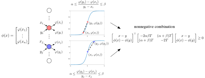
Figure 1: An illustrative description of encoding activation functions by quadratic constraints.

We will see in the next section that the matrix $T$ that parameterizes the multiplier matrix in (9) appears as a decision variable in an SDP, in which the objective is to find an admissible $T$ that yields the tightest bound on the Lipschitz constant.

2.3 LipSDP for single-layer neural network

To develop an optimization problem to estimate the Lipschitz constant of a fully-connected feed-forward neural network, the key insight is that the Lipschitz condition in (1) is in fact equivalent to an incremental quadratic constraint for the map $x\mapsto f(x)$ characterized by the neural network. By coupling this to the incremental quadratic constraints satisfied by the cascade combination of the activation functions [13], we can develop an SDP to minimize an upper bound on the Lipschitz constant of $f$. This result is formally stated in the following theorem.

Theorem 1 (Lipshitz certificates for single-layer neural networks).

Consider a single-layer neural network described by $f(x)=W^{1}\phi(W^{0}x+b^{0})+b^{1}$. Suppose $\phi(x)\colon\mathbb{R}^{n}\to\mathbb{R}^{n}=[\varphi(x_{1})\cdots\varphi(x_{n})]$, where $\varphi$ is slope-restricted in the sector $[\alpha,\beta]$. Define $\mathcal{T}_{n}$ as in (8). Suppose there exists a $\rho>0$ such that the matrix inequality

$$M(\rho,T):=\begin{bmatrix}-2\alpha\beta{W^{0}}^{\top}TW^{0}-\rho I_{n_{0}}&(\alpha+\beta){W^{0}}^{\top}T\\ (\alpha+\beta)TW^{0}&-2T+{W^{1}}^{\top}W^{1}\end{bmatrix}\preceq 0,$$ (10)

holds for some $T\in\mathcal{T}_{n}$. Then $\|f(x)-f(y)\|_{2}\leq\sqrt{\rho}\|x-y\|_{2}$ for all $x,y\in\mathbb{R}^{n_{0}}$.

Theorem 1 provides us with a sufficient condition for $L_{2}=\sqrt{\rho}$ to be an upper bound on the Lipschitz constant of $f(x)=W^{1}\phi(W^{0}x+b^{0})+b^{1}$. In particular, we can find the tightest bound by solving the following optimization problem:

$$\mathrm{minimize}\quad\rho\quad\text{ subject to}\quad M(\rho,T)\preceq 0\quad\text{and}\quad T\in\mathcal{T}_{n},$$ (11)

where the decision variables are $(\rho,T)\in\mathbb{R}_{+}\times\mathcal{T}_{n}$. Note that $M(\rho,T)$ is linear in $\rho$ and $T$ and the set $\mathcal{T}_{n}$ is convex. Hence, (11) is an SDP, which can be solved numerically for its global minimum.

2.4 LipSDP for multi-layer neural networks

We now consider the multi-layer case. Assuming that all the activation functions are the same, we can write the neural network model in (2) compactly as

$$B\mathbf{x}=\phi(A\mathbf{x}+b)\quad\text{and}\quad f(x)=C\mathbf{x}+b^{\ell},$$ (12)

where $\mathbf{x}=[{x^{0}}^{\top}\ {x^{1}}^{\top}\cdots{x^{\ell}}^{\top}]^{\top}$ is the concatenation of the input and the activation values, and the matrices $b$, $A$, $B$ and $C$ are given by [12]

$$A =\begin{bmatrix}W^{0}&0&\ldots&0&0\\ 0&W^{1}&\ldots&0&0\\ \vdots&\vdots&\ddots&\vdots&\vdots\\ 0&0&\ldots&W^{\ell-1}&0\end{bmatrix},\ B=\begin{bmatrix}0&I_{n_{1}}&0&\ldots&0\\ 0&0&I_{n_{2}}&\ldots&0\\ \vdots&\vdots&\vdots&\ddots&\vdots\\ 0&0&0&\ldots&I_{n_{\ell}}\end{bmatrix},$$ (13)

$$C =\begin{bmatrix}0&\ldots&0&W^{\ell}\end{bmatrix},\ b=\begin{bmatrix}{b^{0}}^{\top}&\cdots&{b^{\ell-1}}^{\top}\end{bmatrix}^{\top}.$$

The particular representation in (12) facilitates the extension of LipSDP to multiple layers, as stated in the following theorem.

Theorem 2 (Lipschitz certificates for multi-layer neural networks).

Consider an $\ell$-layer fully connected neural network described by (2). Let $n=\sum_{k=1}^{\ell}n_{k}$ be the total number of hidden neurons and suppose the activation functions are slope-restricted in the sector $[\alpha,\beta]$. Define $\mathcal{T}_{n}$ as in (8). Define $A$ and $B$ as in (13). Consider the matrix inequality

$$M(\rho,T)=\begin{bmatrix}A\\ B\end{bmatrix}^{\top}\begin{bmatrix}-2\alpha\beta T&(\alpha+\beta)T\\ (\alpha+\beta)T&-2T\end{bmatrix}\begin{bmatrix}A\\ B\end{bmatrix}+\begin{bmatrix}-\rho I_{n_{0}}&0&\ldots&0\\ 0&0&\ldots&0\\ \vdots&\vdots&\ddots&\vdots\\ 0&0&\ldots&(W^{\ell})^{\top}W^{\ell}\end{bmatrix}\preceq 0.$$ (14)

If (14) is satisfied for some $(\rho,T)\in\mathbb{R}_{+}\times\mathcal{T}_{n}$, then $\left|\left|f(x)-f(y)\right|\right|_{2}\leq\sqrt{\rho}\left|\left|x-y\right|\right|_{2}$, $\forall x,y\in\mathbb{R}^{n_{0}}$.

In a similar way to the single-layer case, we can find the best bound on the Lipschitz constant by solving the SDP in (11) with $M(\rho,T)$ defined as in (14).

Remark 1.

We have only considered the $\ell_{2}$ norm in our exposition. By using the inequality $\|x\|_{p}\leq n^{\frac{1}{p}-\frac{1}{q}}\|x\|_{q}$, the $\ell_{2}$-Lipschitz bound implies

$$m^{-(\frac{1}{p}-\frac{1}{2})}\|f(y)-f(x)\|_{p}\leq\|f(y)-f(x)\|_{2}\leq L_{2}\|y-x\|_{2}\leq n^{\frac{1}{2}-\frac{1}{q}}L_{2}\|y-x\|_{q},$$

or, equivalently, $\|f(y)-f(x)\|_{p}\leq n^{(\frac{1}{2}-\frac{1}{q})}m^{(\frac{1}{p}-\frac{1}{2})}L_{2}\|y-x\|_{q}.$ Hence, $n^{(\frac{1}{2}-\frac{1}{q})}m^{(\frac{1}{p}-\frac{1}{2})}L_{2}$ is a Lipschitz constant of $f$ when $\ell_{q}$ and $\ell_{p}$ norms are used in the input and output spaces, respectively. We can also extend our framework to accommodate quadratic norms $\|x\|_{P}=\sqrt{x^{\top}Px}$, where $P\in\mathbb{S}_{++}^{n}$.

2.5 Variants of LipSDP: reconciling accuracy and efficiency

In LipSDP, there are $n+1$ decision variables $\rho\geq 0,\ \lambda_{ii},\ 1\leq i\leq n$, where $n$ is the total number of hidden neurons. Using all these decision variables would provide the tightest convex relaxation in our formulation. However, solving this SDP with all the decision variables included is impractical for large networks. Nevertheless, we can consider a hierarchy of relaxations of LipSDP by removing a subset of the decision variables. Below, we give a brief description of the efficiency and accuracy of each variant. Throughout, we let $n$ be the total number of neurons and $\ell$ the number of hidden layers.

1. LipSDP-Neuron has $n+1$ decision variables. For this case, we have $T=\mathrm{diag}(\lambda_{11},\cdots,\lambda_{nn})$.

2. LipSDP-Layer considers only one constraint per layer, resulting in $\ell+1$ decision variables. It is the most scalable and least accurate method. For this variant, we have $T=\mathrm{blkdiag}(\lambda_{1}I_{n_{1}},\cdots,\lambda_{\ell}I_{n_{\ell}})$.

Parallel implementation by splitting. The Lipschitz constant of the composition of two or more functions can be bounded by the product of the Lispchtiz constants of the individual functions. By splitting a neural network up into small sub-networks, one can first bound the Lipschitz constant of each sub-network and then multiply these constants together to obtain a Lipschitz constant for the entire network. Because sub-networks do not share weights, it is possible to compute the Lipschitz constants for each sub-network in parallel. This greatly improves the scalability of of each variant of LipSDP with respect to the total number of activation functions in the network.

Repeated nonlinearities. The quadratic constraint in Lemma 1 is valid for functions of the form $\phi(x)=[\varphi_{1}(x_{1})\cdots\varphi_{n}(x_{n})]^{\top}$ as along as all $\varphi_{i}$’s are slope-restricted on $[\alpha,\beta]$. Therefore, this quadratic constraint does not exploit the fact that the same activation functions are used. In Appendix A.8 we derive more refined quadratic constraints that exploit this additional structure when one of the points in the definition of Lipschitz continuity is fixed. The resulting SDP would be tighter but more expensive to solve.

3 Experiments

$n$	LipSDP- Neuron	LipSDP- Layer
500	5.22	2.85
1000	27.91	17.88
1500	82.12	58.61
2000	200.88	146.09
2500	376.07	245.94
3000	734.63	473.25

Table 1: Computation time in seconds for evaluating Lipschitz bounds of one-hidden-layer neural networks with a varying number of hidden units. A plot showing the Lipschitz constant for each network tested in this table has been provided in the Appendix.

$\ell$	LipSDP- Neuron	LipSDP- Layer
5	20.33	3.41
10	32.18	7.06
50	87.45	25.88
100	135.85	40.39
200	221.2	64.90
500	707.56	216.49

Table 2: Computation time in seconds for computing Lipschitz bounds of $\ell$-hidden-layer neural networks with 100 activation functions per layer. For LipSDP-Neuron and LipSDP-Layer, we split each network up into 5-layer sub-networks.

In this section we describe several experiments that highlight the key aspects of this work. In particular, we show empirically that our bounds are much tighter than any comparable method, we study the impact of robust training on our Lipschitz bounds, and we analyze the scalability of our methods.

Experimental setup. For our experiments we used MATLAB, the CVX toolbox [16] and MOSEK [2] on a 9-core CPU with 16GB of RAM to solve the SDPs. All classifiers trained on MNIST used an 80-20 train-test split.

Training procedures. Several training procedures have recently been proposed to improve the robustness of neural network classifiers. Two prominent procedures are the LP-based method in [20] and projected gradient descent (PGD) based method in [23]. We refer to these training methods as LP-Train and PGD-Train, respectively. Both procedures take as input a parameter $\epsilon$ that defines the $\ell_{\infty}$ perturbation of the training data points.

Baselines. Throughout the experiments, we will often show comparisons to what we call the naive lower and upper bounds. As has been shown in several previous works [9, 36], trivial lower and upper bounds on the Lipschitz constant of a feed-forward neural network with $\ell$ hidden-layers are given by $L_{2,\text{ lower}}=\left|\left|W^{\ell}W^{\ell-1}\cdots W^{0}\right|\right|_{2}$ and $L_{2,\text{ upper}}=\prod_{i=0}^{\ell}\left|\left|W^{i}\right|\right|_{2}$, which we refer to them as naive lower and upper bounds, respectively. We are aware of only two methods that bound the Lipschitz constant and can scale to fully-connected networks with more than two hidden layers; these methods are [9], which we will refer to as CPLip, and [36], which is called SeqLip.

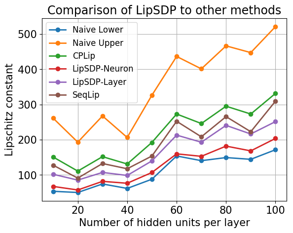
(a) Comparison of Lipschitz bounds found by various methods for five-hidden-layer networks trained on MNIST with the Adam optimizer. Each network had a test accuracy above 97%.

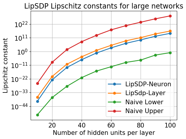
(b) Lipschitz bounds obtained by splitting a 100-layer network into sub-networks. Each sub-network had six layers, and the weights were generated randomly by sampling from a normal distribution.

Figure 2: Comparison of the accuracy LipSDP methods to other methods that compute the Lipschitz constant and scalability analysis of all three SeqLip methods.

We compare the Lipschitz bounds obtained by LipSDP-Neuron, LipSDP-Layer, CPLip, and SeqLip in Figure 2(a). It is evident from this figure that the bounds from LipSDP-Neuron are tighter than CPLip and SeqLip. Our results show that the true Lipschitz constants of the networks shown above are very close to the naive lower bound.

To demonstrate the scalability of the LipSDP formulations, we split a 100-hidden layer neural network into sub-networks with six hidden layers each and computed the Lipschitz bounds using LipSDP-Neuron and LipSDP-Layer. The results are shown in Figure 2(b). Furthermore, in Tables 1 and 2, we show the computation time for scaling the LipSDP methods in the number of hidden units per layer and in the number of layers. In particular, the largest network we tested in Table 2 had 50,000 hidden neurons; SDPLip-Neuron took approximately 12 minutes to find a Lipschitz bound, and SDPLip-Layer took approximately 4 minutes.

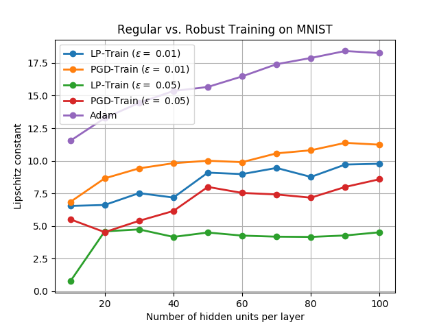
(a) Lipschitz bounds for a one-hidden-layer neural networks trained on the MNIST dataset with the Adam optimizer and LP-Train and PGD-Train for two values of the robustness parameter $\epsilon$. Each network reached an accuracy of 95% or higher.

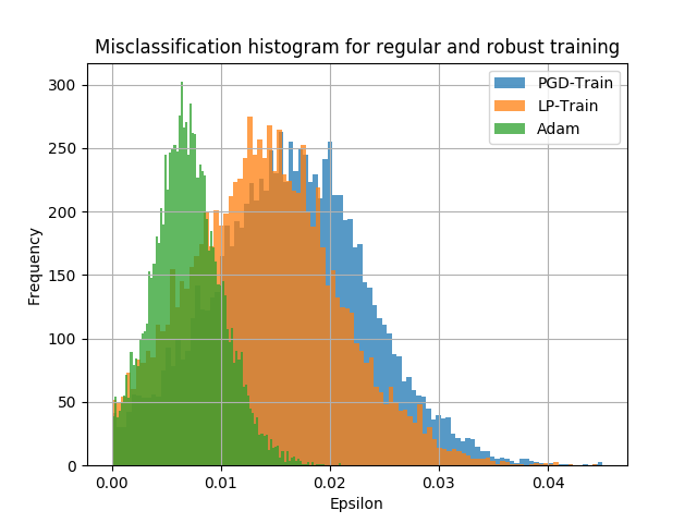
Figure 3: Histograms showing the local robustness (in $\ell_{\infty}$ norm) around each correctly-classified test instance from the MNIST dataset. The neural networks had three hidden layers with 100, 50, 20 neurons, respectively. All classifiers had a test accuracy of 97%.

Figure 4: Analysis of impact of robust training on the Lipschitz constant and the distance to misclassification for networks trained on MNIST

Impact of robust training. In Figure 4, we empirically demonstrate that the Lipschitz bound of a neural network is directly related to the robustness of the corresponding classifier. This figure shows that LP-train and PGD-Train networks achieve lower Lipschitz bounds than standard training procedures. Figure 3(a) indicates that robust training procedures yield lower Lipschitz constants than networks trained with standard training procedures such as the Adam optimizer. Figure 3 shows the utility of sharply estimating the Lipschitz constant; a lower value of $L_{2}$ guarantees that a neural network is more locally robust to input perturbations; see Proposition 1 in the Appendix.

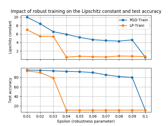
Figure 5: Trade-off between accuracy and Lipschitz constant for different values of the robustness parameter used for LP-Train and PGD-Train. All networks had one hidden layer with 50 hidden neurons.

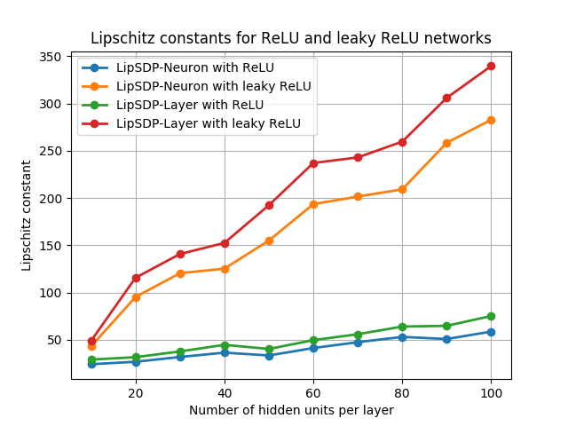
Figure 6: Lipschitz constants for topologically identical three-hidden-layer networks with ReLU and leaky ReLU activation functions. All classifiers were trained until they reached 97% test accuracy.

In the same vein, Figure 3 shows the impact of varying the robustness parameter $\epsilon$ used in LP-Train and PGD-Train on the test accuracy of networks trained for a fixed number of epochs and the corresponding Lipschitz constants. In essence, these results quantify how much robustness a fixed classifier can handle before accuracy plummets. Interestingly, the drops in accuracy as $\epsilon$ increases coincide with corresponding drops in the Lipschitz constant for both LP-Train and PGD-Train.

Robustness for different activation functions. The framework proposed in this work allows us to examine the impact of using different activation functions on the Lipschitz constant of neural networks. We trained two sets of neural networks on the MNIST dataset. The first set used ReLU activation functions, while the second set used leaky ReLU activations. Figure 6 shows empirically that the networks with the leaky ReLU activation function have larger Lipschitz constants than networks of the same architecture with the ReLU activation function.

4 Conclusions and future work

In this paper, we proposed a hierarchy of semidefinite programs to derive tight upper bounds on the Lipschitz constant of feed-forward fully-connected neural networks. Some comments are in order. First, our framework can be directly used to certify convolutional neural networks (CNNs) by unrolling them to a large feed-forward neural network. A future direction is to exploit the special structure of CNNs in the resulting SDP. Second, we only considered one application of Lipschitz bounds in depth (robustness certification). Having an accurate upper bound on the Lipschitz constant can be useful in domains beyond robustness analysis, such as stability analysis of feedback systems with control policies updated by deep reinforcement learning. Furthermore, Lipschitz bounds can be utilized during training as a heuristic to promote out-of-sample generalization [35]. We intend to pursue these applications for future work.

Appendix A Appendix

A.1 Robustness certification of DNN-based classifiers

Consider a classifier described by a feed-forward neural network $f\colon\mathbb{R}^{n}\to\mathbb{R}^{k}$, where $n$ is the number of input features and $k$ is the number of classes. In this context, the function $f$ takes as input an instance or measurement $x$ and returns a $k$-dimensional vector of scores – one for each class. The classification rule is based on assigning $x$ to the class with the highest score. That is, we define the classification $C(x):\mathbb{R}^{n}\rightarrow\{1,\dots,k\}$ to be $C(x)=\mathrm{argmax}_{1\leq i\leq k}\ f_{i}(x)$. Now suppose that $x^{\star}$ is an instance that is classified correctly by the neural network. To evaluate the local robustness of the neural network around $x^{\star}$, we consider a bounded set $\mathcal{A}(x^{\star})=\{x\mid\|x-x^{\star}\|_{2}\leq\epsilon\}\subseteq\mathbb{R}^{n}$ that represents the set of all possible $\ell_{2}$-norm perturbations of $x^{\star}$. Then the classifier is locally robust at $x^{\star}$ against $\mathcal{A}(x^{\star})$ if it assigns all the perturbed inputs to the same class as the unperturbed input, i.e., if

$$C(x)=C(x^{\star})\quad\forall x\in\mathcal{A}(x^{\star}).$$ (15)

In the following proposition, we derive a sufficient condition to guarantee local robustness around $x^{\star}$ for the perturbation set $\mathcal{A}(x^{\star})$.

Proposition 1.

Consider a neural-network classifier $f\colon\mathbb{R}^{n}\to\mathbb{R}^{k}$ with Lipschitz constant $L_{2}$ in the $\ell_{2}$-norm. Let $\epsilon>0$ be given and consider the inequality

$$L_{2}\leq\frac{1}{\epsilon\sqrt{2}}\min_{1\leq j\leq k,\ j\neq i^{\star}}\ |f_{j}(x^{\star})-f_{i^{\star}}(x^{\star})|.$$ (16)

Then (16) implies $C(x):=\mathrm{argmax}_{1\leq i\leq k}f_{i}(x)=C(x^{\star})$ for all $x\in\mathcal{A}(x^{\star})$.

The inequality in (16) provides us with a simple and computationally efficient test for assessing the point-wise robustness of a neural network. According to (16), a more accurate estimation of the Lipschitz constant directly increases the maximum perturbation $\epsilon$ that can be certified for each test example. This makes the framework suitable for model selection, wherein one wishes to select the model that is most robust to adversarial perturbations from a family of proposed classifiers [26].

A.2 Proof of Proposition 1

Let $i^{\star}=\mathrm{argmax}_{1\leq i\leq k}\ f_{i}(x^{\star})$ be the class of $x^{\star}$. Define the polytope in the output space of $f$:

$$\mathcal{P}_{i^{\star}}=\{y\mid(e_{j}-e_{i^{\star}})^{\top}y\leq 0\quad 1\leq j\leq k,\ j\neq i^{\star}\}.$$

which is the set of all outputs whose score is the highest for class $i^{\star}$; and, of course, $f(x^{\star})\in\mathcal{P}_{i^{\star}}$. The distance of $f(x^{\star})$ to the boundary $\partial\mathcal{P}_{i}$ of the polytope is the minimum distance of $f(x^{\star})$ to all edges of the polytope:

$$\mathbf{dist}(f(x^{\star}),\partial\mathcal{P}_{i^{\star}})=\inf_{y\in\partial\mathcal{P}_{i^{\star}}}\|y-f(x^{\star})\|_{2}=\frac{1}{\sqrt{2}}\min_{1\leq j\leq k,\ j\neq i^{\star}}\ |f_{j}(x^{\star})-f_{i^{\star}}(x^{\star})|.$$

Note that the Lipschitz condition implies $\mathbf{dist}(f(x^{\star}),f(x))=\|f(x)-f(x^{\star})\|_{2}\leq L_{2}\epsilon$ for all $\|x-x^{\star}\|_{2}\leq\epsilon$. The condition in (16) then implies

$$\mathbf{dist}(f(x^{\star}),f(x))\leq\mathbf{dist}(f(x^{\star}),\partial\mathcal{P}_{i^{\star}})\ \text{ for all }\|x-x^{\star}\|_{2}\leq\epsilon,$$

and for all $1\leq j\leq k,\ j\neq i^{\star}$. Therefore, the output of the classification would not change for any $\|x-x^{\star}\|_{2}\leq\epsilon$.

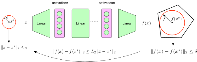
Figure 7: Illustration of local robustness certification using the Lipschitz bound.

A.3 Proof of Lemma 1

Let $T=\mathrm{diag}(\lambda_{11},\cdots,\lambda_{nn})$ with $\lambda_{ii}\geq 0$ for all $1\leq i\leq n$. By expanding the quadratic form on the right-hand side of (9), we can write

$$-2\alpha\beta(x\!-\!y)^{\top}T(x-y)+2(\alpha+\beta)(x\!-\!y)^{\top}T(\phi(x)\!-\!\phi(y))-2(\phi(x)\!-\!\phi(y))^{\top}T(\phi(x)\!-\!\phi(y))$$

$$=\sum_{i=1}^{n}\lambda_{ii}\left(-2\alpha\beta(x_{i}-y_{i})^{2}+2(\alpha+\beta)(x_{i}-y_{i})(\varphi(x_{i})-\varphi(y_{i}))-2(\varphi(x_{i})-\varphi(y_{i}))^{2}\right)$$

$$=\sum_{i=1}^{n}\lambda_{ii}\begin{bmatrix}x_{i}-y_{i}\\ \varphi(x_{i})-\varphi(y_{i})\end{bmatrix}^{\top}\begin{bmatrix}-2\alpha\beta&\alpha+\beta\\ \alpha+\beta&-2\end{bmatrix}\begin{bmatrix}x_{i}-y_{i}\\ \varphi(x_{i})-\varphi(y_{i})\end{bmatrix}\geq 0,$$

where the last inequality follows from (7).

A.4 Proof of Theorem 1

Define $x^{1}=\phi(W^{0}x+b^{0})\in\mathbb{R}^{n}$ and $y^{1}=\phi(W^{0}y+b^{0})\in\mathbb{R}^{n}$ for two arbitrary inputs $x,y\in\mathbb{R}^{n_{0}}$. Using Lemma 1, we can write the quadratic inequality

$$0\leq\begin{bmatrix}(W^{0}x+b^{0})-(W^{0}y+b^{0})\\ x^{1}-y^{1}\end{bmatrix}^{\top}\begin{bmatrix}-2\alpha\beta T&(\alpha+\beta)T\\ (\alpha+\beta)T&-2T\end{bmatrix}\begin{bmatrix}(W^{0}x+b^{0})-(W^{0}y+b^{0})\\ x^{1}-y^{1}\end{bmatrix},$$

where $T\in\mathcal{T}_{n}$ and $\mathcal{T}_{n}$ is defined as in (8). The preceding inequality can be simplified to

$$0\leq\begin{bmatrix}x\!-\!y\\ x^{1}\!-\!y^{1}\end{bmatrix}^{\top}\begin{bmatrix}-2\alpha\beta{W^{0}}^{\top}TW^{0}&(\alpha+\beta){W^{0}}^{\top}T\\ (\alpha+\beta)TW^{0}&-2T\end{bmatrix}\begin{bmatrix}x\!-\!y\\ x^{1}\!-\!y^{1}\end{bmatrix}.$$ (17)

By left and right multiplying $M(\rho,T)$ in (10) by $\begin{bmatrix}(x\!-\!y)^{\top}&(x^{1}\!-\!y^{1})^{\top}\end{bmatrix}$ and $\begin{bmatrix}(x\!-\!y)^{\top}&(x^{1}\!-\!y^{1})^{\top}\end{bmatrix}^{\top}$, respectively, and rearranging terms, we obtain

$$\begin{bmatrix}x\!-\!y\\ x^{1}\!-\!y^{1}\end{bmatrix}^{\top}\begin{bmatrix}-2\alpha\beta{W^{0}}^{\top}TW^{0}&(\alpha+\beta){W^{0}}^{\top}T\\ (\alpha+\beta)TW^{0}&-2T\end{bmatrix}\begin{bmatrix}x\!-\!y\\ x^{1}\!-\!y^{1}\end{bmatrix}$$ (18)

$$\leq\begin{bmatrix}x\!-\!y\\ x^{1}\!-\!y^{1}\end{bmatrix}^{\top}\begin{bmatrix}L_{2}^{2}I_{n_{0}}&0\\ 0&-{W^{1}}^{\top}W^{1}\end{bmatrix}\begin{bmatrix}x\!-\!y\\ x^{1}\!-\!y^{1}\end{bmatrix}.$$

By adding both sides of the preceding inequalities, we obtain

$$0\leq\begin{bmatrix}x\!-\!y\\ x^{1}\!-\!y^{1}\end{bmatrix}^{\top}\begin{bmatrix}L_{2}^{2}I_{n_{0}}&0\\ 0&-{W^{1}}^{\top}W^{1}\end{bmatrix}\begin{bmatrix}x\!-\!y\\ x^{1}\!-\!y^{1}\end{bmatrix},$$

or, equivalently,

$$(x^{1}-y^{1})^{\top}{W^{1}}^{\top}W^{1}(x^{1}-y^{1})\leq L_{2}^{2}(x-y)^{\top}(x-y).$$

Finally, note that by definition of $x^{1}$ and $y^{1}$, we have $f(x)=W^{1}x^{1}+b^{1}$ and $f(y)=W^{1}y^{1}+b^{1}$. Therefore, the preceding inequality implies

$$\|f(x)-f(y)\|_{2}\leq L_{2}\|x-y\|_{2}\quad\text{for all }x,y\in\mathbb{R}^{n_{0}}.$$ (19)

A.5 Proof of Theorem 2

For two arbitrary inputs $x^{0},y^{0}\in\mathbb{R}^{n_{0}}$, define $\mathbf{x}=[{x^{0}}^{\top}\cdots{x^{\ell}}^{\top}]^{\top}\quad\text{ and }\quad\mathbf{y}=[{y^{0}}^{\top}\cdots{y^{\ell}}^{\top}]^{\top}$ Using the compact notation in (12), we can write

$$B\mathbf{x} =\phi(A\mathbf{x}+b)\quad\text{ and }\quad B\mathbf{y}=\phi(A\mathbf{y}+b).$$

Multiply both sides of the first matrix in (14) by $(\mathbf{x}-\mathbf{y})^{\top}$ and $(\mathbf{x}-\mathbf{y})$, respectively and use the preceding identities to obtain

$$(\mathbf{x}-\mathbf{y})^{\top}\begin{bmatrix}A\\ B\end{bmatrix}^{\top}\begin{bmatrix}-2\alpha\beta T&(\alpha+\beta)T\\ (\alpha+\beta)T&-2T\end{bmatrix}\begin{bmatrix}A\\ B\end{bmatrix}(\mathbf{x}-\mathbf{y})$$ (20)

$$=\begin{bmatrix}A\mathbf{x}-A\mathbf{y}\\ B\mathbf{x}-B\mathbf{y}\end{bmatrix}^{\top}\begin{bmatrix}-2\alpha\beta T&(\alpha+\beta)T\\ (\alpha+\beta)T&-2T\end{bmatrix}\begin{bmatrix}A\mathbf{x}-A\mathbf{y}\\ B\mathbf{x}-B\mathbf{y}\end{bmatrix}$$

$$=\begin{bmatrix}A\mathbf{x}-A\mathbf{y}\\ \phi(A\mathbf{x}+b)-\phi(A\mathbf{y}+b)\end{bmatrix}^{\top}\begin{bmatrix}-2\alpha\beta T&(\alpha+\beta)T\\ (\alpha+\beta)T&-2T\end{bmatrix}\begin{bmatrix}A\mathbf{x}-A\mathbf{y}\\ \phi(A\mathbf{x}+b)-\phi(A\mathbf{y}+b)\end{bmatrix}\geq 0,$$

where the last inequality follows from Lemma 1. On the other hand, by multiplying both sides of the second matrix in (14) by $(\mathbf{x}-\mathbf{y})^{\top}$ and $(\mathbf{x}-\mathbf{y})$, respectively, we can write

$$(\mathbf{x}-\mathbf{y})^{\top}M(\mathbf{x}-\mathbf{y})=\|f(x)-f(y)\|_{2}^{2}-L_{2}^{2}\|x-y\|_{2}^{2},$$ (21)

where we have used the fact that $f(x)=W^{\ell}x^{\ell}+b^{\ell}$ and $f(y)=W^{\ell}y^{\ell}+b^{\ell}$. By adding both sides of (20) and (21), we get

$$(\mathbf{x}-\mathbf{y})^{\top}\left(\begin{bmatrix}A\\ B\end{bmatrix}^{\top}\begin{bmatrix}-2\alpha\beta T&(\alpha+\beta)T\\ (\alpha+\beta)T&-2T\end{bmatrix}\begin{bmatrix}A\\ B\end{bmatrix}+M\right)(\mathbf{x}-\mathbf{y})\geq\|f(x)-f(y)\|_{2}^{2}-L_{2}^{2}\|x-y\|_{2}^{2}.$$ (22)

When the LMI in (14) holds, the left-hand side of (22) is non-positive, implying that the right-hand side is non-positive.

A.6 Bounding the output set of a neural network classifier

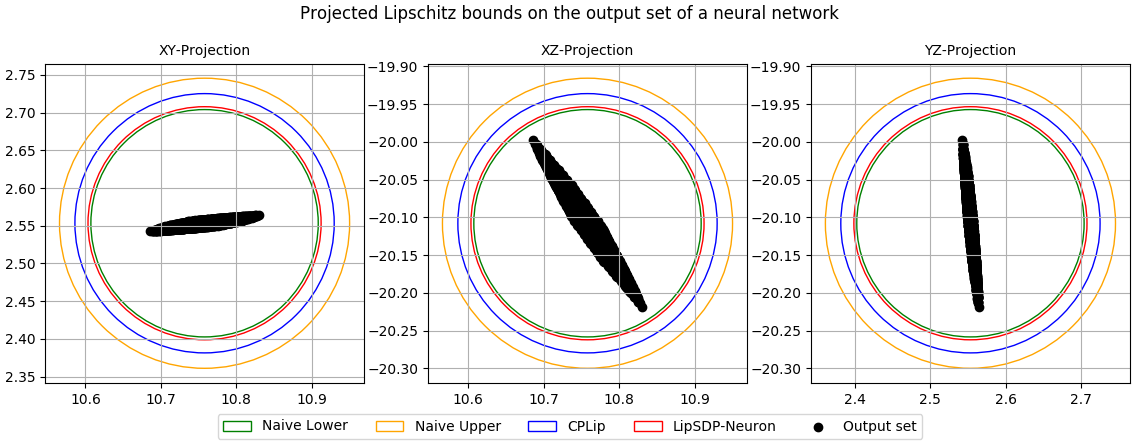
Figure 8: Bounds on the image of an $\ell_{2}$ $0.01$-ball under a neural network trained on the Iris dataset. The network was trained using the Adam optimizer and reached a test accuracy of 99%.

As we have shown, accurate estimation of the Lipschitz constant can provide tighter bounds on adversarial examples drawn from a perturbation set around a nominal point $\bar{x}$. Figure 8 shows these bounds for a neural network trained on the Iris dataset. Because this dataset has three classes, we project the output sets onto the coordinate axes. This figure clearly shows that our bound is quite close to the naive lower bound. Indeed, the naive upper bound and the constant computed by CPLip are considerably looser.

A.7 Further analysis of scalability

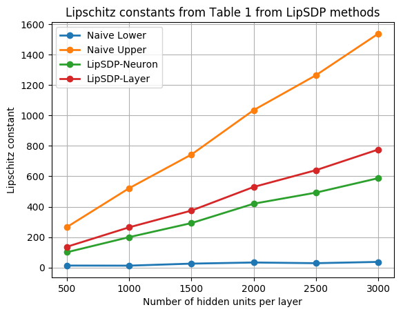
Figure 9: Lipschitz bounds for networks in Table 1.

Figure 9 shows the Lipschitz bounds found for the networks used in Table 1.

A.8 LipSDP and repeated nonlinearities

The incremental quadratic constraint in Lemma 1 is valid for functions of the form $\phi(x)=[\varphi_{1}(x_{1})\cdots\varphi_{n}(x_{n})]^{\top}$ as along as all $\varphi_{i}$’s are slope-restricted on $[\alpha,\beta]$. Therefore, this quadratic constraint does not exploit the fact that the same activation functions are used. In this subsection, we derive more refined quadratic constraints that exploit this additional structure when one of the points in the definition of Lipschitz continuity is fixed. Explicity, for a given $y\in\mathbb{R}^{n_{0}}$, our goal is to compute the smallest $\rho$ (depending on $y$) such that

$$\|f(x)-f(y)\|_{2}\leq\sqrt{\rho}\|x-y\|_{2}\quad\forall x\in\mathbb{R}^{n_{0}}$$ (23)

This inequality can be equivalently written as

$$\begin{bmatrix}x\\ f(x)\\ 1\end{bmatrix}^{\top}\underbrace{\begin{bmatrix}-\rho I_{n_{0}}&0&\rho y\\ 0&I_{n_{f}}&-f(y)\\ \rho y^{\top}&-f(y)^{\top}&f(y)^{\top}f(y)-\rho y^{\top}y\end{bmatrix}}_{R(\rho)}\begin{bmatrix}x\\ f(x)\\ 1\end{bmatrix}\leq 0\quad\forall x\in\mathbb{R}^{n_{0}}$$ (24)

To certify the quadratic inequality above, we make use of the following definition from [12].

Definition 3.

Let $\phi\colon\mathbb{R}^{n}\to\mathbb{R}^{n}$ and suppose $\mathcal{Q}\subset\mathbb{S}^{2n+1}$ is the set of all symmetric and indefinite matrices $Q$ such that the inequality

$$\begin{bmatrix}x\\ \phi(x)\\ 1\end{bmatrix}^{\top}Q\begin{bmatrix}x\\ \phi(x)\\ 1\end{bmatrix}\geq 0,$$ (25)

holds for all $x\in\mathcal{X}\subseteq\mathbb{R}^{n}$. Then we say $\phi$ satisfies the quadratic constraint defined by $\mathcal{Q}$ on $\mathcal{X}$.

Note that Quadratic Constraints as defined above are more general than Incremental Quadratic Constraints, and would allow us to capture more information about $\phi$. For example, for any pair $(x_{i},x_{j})\ i\neq j$, since $\varphi(x_{i})$ and $\varphi(x_{j})$ are obtained from the same nonlinearity, we can write the incremental quadratic constraint

$$\begin{bmatrix}x_{i}-x_{j}\\ \varphi(x_{i})-\varphi(x_{j})\end{bmatrix}^{\top}\begin{bmatrix}-2\alpha\beta&\alpha+\beta\\ \alpha+\beta&-2\end{bmatrix}\begin{bmatrix}x_{i}-x_{j}\\ \varphi(x_{i})-\varphi(x_{j})\end{bmatrix}\geq 0\quad 1\leq i<j\leq n,$$

This inequality can be equivalently represented as

$$\begin{bmatrix}x_{i}\\ x_{j}\\ \varphi(x_{i})\\ \varphi(x_{j})\\ 1\end{bmatrix}^{\top}\begin{bmatrix}-2\alpha\beta&2\alpha\beta&\alpha+\beta&-(\alpha+\beta)&0\\ 2\alpha\beta&-2\alpha\beta&-(\alpha+\beta)&\alpha+\beta&0\\ \alpha+\beta&-(\alpha+\beta)&-2&2&0\\ -(\alpha+\beta)&\alpha+\beta&2&-2&0\\ 0&0&0&0&0\end{bmatrix}\begin{bmatrix}x_{i}\\ x_{j}\\ \varphi(x_{i})\\ \varphi(x_{j})\\ 1\end{bmatrix}\geq 0,$$ (26)

This quadratic constraints couples neuron $i$ and $j$, $i\neq j$, resulting in $O(n^{2})$ quadratic constraints for an activation layer with $n$ neurons. In the following lemma, we characterize $\phi(x)=[\varphi(x_{1})\cdots\varphi(x_{n})]^{\top}$ with all possible incremental quadratic constraints.

Lemma 2 (Lemma 2 of [12]).

Suppose $\varphi\colon\mathbb{R}\to\mathbb{R}$ is slope-restricted on $[\alpha,\beta]$. Define the set

$$\mathcal{S}_{n}=\left\{S\in\mathbb{S}^{n}\mid S\!=\!\!\sum_{1\leq i<j\leq n}\lambda_{ij}(e_{i}\!-\!e_{j})(e_{i}\!-\!e_{j})^{\top},\ \lambda_{ij}\geq 0\right\}.$$ (27)

where $e_{i}$ is the $i$-th standard basis vector in $\mathbb{R}^{n}$. Then for any $S\in\mathcal{S}_{n}$ the vector-valued function $\phi:\mathbb{R}^{n}\rightarrow\mathbb{R}^{n}$ defined by $\phi(x)=[\varphi(x_{1})\cdots\varphi(x_{n})]^{\top}$ satisfies

$$\begin{bmatrix}x\\ \phi(x)\\ 1\end{bmatrix}^{\top}\begin{bmatrix}-2\alpha\beta S&(\alpha+\beta)S&0\\ (\alpha+\beta)S&-2S&0\\ 0&0&0\end{bmatrix}\begin{bmatrix}x\\ \phi(x)\\ 1\end{bmatrix}\geq 0\ \text{ for all }x,y\in\mathbb{R}^{n}.$$ (28)

In the above Lemma, we are only capturing the quadratic constraints implied by slope restriction that are imposed between any pair of neurons. However, depending on what activation function is being considered, more quadratic constraints can be included. For a detailed account of Quadratic Constraints, see [12].

LipSDP with repeated nonlinearities.

Consider the compact representation (12) of a multi-layer network $f$ defined by the recursion (2). Suppose $\phi$ satisfies the quadratic constraint defined by $\mathcal{Q}$ on $\mathbb{R}^{n}$. Utilizing Definition 3, we can write the following quadratic constraints for any $Q\in\mathcal{Q}$,

$$\begin{bmatrix}A\mathbf{x}+b\\ B\mathbf{x}\\ 1\end{bmatrix}^{\top}Q\begin{bmatrix}A\mathbf{x}+b\\ B\mathbf{x}\\ 1\end{bmatrix}=\begin{bmatrix}\mathbf{x}\\ 1\end{bmatrix}^{\top}\begin{bmatrix}A&b\\ B&0\\ 0&1\end{bmatrix}^{\top}Q\begin{bmatrix}A&b\\ B&0\\ 0&1\end{bmatrix}\begin{bmatrix}\mathbf{x}\\ 1\end{bmatrix}\geq 0,\quad\forall\mathbf{x}$$ (29)

Now consider the following LMI,

$$N(\rho,T)\!:=\!\begin{bmatrix}A&b\\ B&0\\ 0&1\end{bmatrix}^{\top}Q\begin{bmatrix}A&b\\ B&0\\ 0&1\end{bmatrix}\!+\!\begin{bmatrix}I_{n_{0}}&0&0\\ 0&0&0\\ \vdots&\vdots&\vdots\\ 0&{W^{\ell}}^{\top}&0\\ 0&{b^{\ell}}^{\top}&1\end{bmatrix}R(\rho)\begin{bmatrix}I_{n_{0}}&0&0\\ 0&0&0\\ \vdots&\vdots&\vdots\\ 0&{W^{\ell}}^{\top}&0\\ 0&{b^{\ell}}^{\top}&1\end{bmatrix}^{\top}\preceq 0,$$ (30)

where $R(\rho)$ is defined in (23). By left- and right- multiplying both sides by $\begin{bmatrix}\mathbf{x}^{\top}&1\end{bmatrix}$ and $\begin{bmatrix}\mathbf{x}^{\top}&1\end{bmatrix}^{\top}$, respectively, we obtain

$$\begin{bmatrix}\mathbf{x}\\ 1\end{bmatrix}^{\top}\left(\begin{bmatrix}A&b\\ B&0\\ 0&1\end{bmatrix}^{\top}Q\begin{bmatrix}A&b\\ B&0\\ 0&1\end{bmatrix}\!+\!\begin{bmatrix}I_{n_{0}}&0&0\\ 0&0&0\\ \vdots&\vdots&\vdots\\ 0&{W^{\ell}}^{\top}&0\\ 0&{b^{\ell}}^{\top}&1\end{bmatrix}R(\rho)\begin{bmatrix}I_{n_{0}}&0&0\\ 0&0&0\\ \vdots&\vdots&\vdots\\ 0&{W^{\ell}}^{\top}&0\\ 0&{b^{\ell}}^{\top}&1\end{bmatrix}^{\top}\right)\begin{bmatrix}\mathbf{x}\\ 1\end{bmatrix}\leq 0.$$

The first term is non-negative by (29), implying that the second term is non-positive. Therefore,

$$\begin{bmatrix}\mathbf{x}\\ 1\end{bmatrix}^{\top}\begin{bmatrix}I_{n_{0}}&0&0\\ 0&0&0\\ \vdots&\vdots&\vdots\\ 0&{W^{\ell}}^{\top}&0\\ 0&{b^{\ell}}^{\top}&1\end{bmatrix}R(\rho)\begin{bmatrix}I_{n_{0}}&0&0\\ 0&0&0\\ \vdots&\vdots&\vdots\\ 0&{W^{\ell}}^{\top}&0\\ 0&{b^{\ell}}^{\top}&1\end{bmatrix}^{\top}\begin{bmatrix}\mathbf{x}\\ 1\end{bmatrix}\!=\begin{bmatrix}x^{0}\\ f(x^{0})\\ 1\end{bmatrix}^{\top}R(\rho)\begin{bmatrix}x^{0}\\ f(x^{0})\\ 1\end{bmatrix}\leq 0$$

Therefore, the feasibility of the LMI in (30) implies the inequality in (23). We remark that the LMI in (30) has now $O(n^{2})$ decision variables. For future work, we will invesitigate the effectiveness of these additional decision variables on the computed Lipschitz bound.

References

- [1] Behçet Açıkmeşe and Martin Corless. Observers for systems with nonlinearities satisfying incremental quadratic constraints. Automatica, 47(7):1339–1348, 2011.
- [2] MOSEK ApS. The MOSEK optimization toolbox for MATLAB manual. Version 8.1., 2017.
- [3] Anil Aswani, Humberto Gonzalez, S Shankar Sastry, and Claire Tomlin. Provably safe and robust learning-based model predictive control. Automatica, 49(5):1216–1226, 2013.
- [4] Radu Balan, Maneesh Singh, and Dongmian Zou. Lipschitz properties for deep convolutional networks. arXiv preprint arXiv:1701.05217, 2017.
- [5] Peter L Bartlett, Dylan J Foster, and Matus J Telgarsky. Spectrally-normalized margin bounds for neural networks. In Advances in Neural Information Processing Systems, pages 6240–6249, 2017.
- [6] Osbert Bastani, Yani Ioannou, Leonidas Lampropoulos, Dimitrios Vytiniotis, Aditya Nori, and Antonio Criminisi. Measuring neural net robustness with constraints. In Advances in neural information processing systems, pages 2613–2621, 2016.
- [7] Felix Berkenkamp, Matteo Turchetta, Angela Schoellig, and Andreas Krause. Safe model-based reinforcement learning with stability guarantees. In Advances in neural information processing systems, pages 908–918, 2017.
- [8] Stephen Boyd and Lieven Vandenberghe. Convex optimization. Cambridge university press, 2004.
- [9] Patrick L. Combettes and Jean-Christophe Pesquet. Lipschitz certificates for neural network structures driven by averaged activation operators. arXiv preprint arXiv:1903.01014, 2019.
- [10] Dheeru Dua and Casey Graff. UCI machine learning repository, 2017.
- [11] Souradeep Dutta, Susmit Jha, Sriram Sankaranarayanan, and Ashish Tiwari. Output range analysis for deep feedforward neural networks. In NASA Formal Methods Symposium, pages 121–138. Springer, 2018.
- [12] Mahyar Fazlyab, Manfred Morari, and George J Pappas. Safety verification and robustness analysis of neural networks via quadratic constraints and semidefinite programming. arXiv preprint arXiv:1903.01287, 2019.
- [13] Mahyar Fazlyab, Alejandro Ribeiro, Manfred Morari, and Victor M Preciado. Analysis of optimization algorithms via integral quadratic constraints: Nonstrongly convex problems. SIAM Journal on Optimization, 28(3):2654–2689, 2018.
- [14] Timon Gehr, Matthew Mirman, Dana Drachsler-Cohen, Petar Tsankov, Swarat Chaudhuri, and Martin Vechev. Ai2: Safety and robustness certification of neural networks with abstract interpretation. In 2018 IEEE Symposium on Security and Privacy (SP), pages 3–18. IEEE, 2018.
- [15] Ian J Goodfellow, Jonathon Shlens, and Christian Szegedy. Explaining and harnessing adversarial examples (2014). arXiv preprint arXiv:1412.6572.
- [16] Michael Grant, Stephen Boyd, and Yinyu Ye. Cvx: Matlab software for disciplined convex programming, 2008.
- [17] Todd Huster, Cho-Yu Jason Chiang, and Ritu Chadha. Limitations of the lipschitz constant as a defense against adversarial examples. In Joint European Conference on Machine Learning and Knowledge Discovery in Databases, pages 16–29. Springer, 2018.
- [18] Ming Jin and Javad Lavaei. Stability-certified reinforcement learning: A control-theoretic perspective. arXiv preprint arXiv:1810.11505, 2018.
- [19] Matt Jordan, Justin Lewis, and Alexandros G Dimakis. Provable certificates for adversarial examples: Fitting a ball in the union of polytopes. arXiv preprint arXiv:1903.08778, 2019.
- [20] J Zico Kolter and Eric Wong. Provable defenses against adversarial examples via the convex outer adversarial polytope. arXiv preprint arXiv:1711.00851, 1(2):3, 2017.
- [21] Alexey Kurakin, Ian Goodfellow, and Samy Bengio. Adversarial machine learning at scale. arXiv preprint arXiv:1611.01236, 2016.
- [22] Yann LeCun. The mnist database of handwritten digits. http://yann. lecun. com/exdb/mnist/, 1998.
- [23] Aleksander Madry, Aleksandar Makelov, Ludwig Schmidt, Dimitris Tsipras, and Adrian Vladu. Towards deep learning models resistant to adversarial attacks. arXiv preprint arXiv:1706.06083, 2017.
- [24] Yurii Nesterov. Introductory lectures on convex optimization: A basic course, volume 87. Springer Science & Business Media, 2013.
- [25] Nicolas Papernot, Patrick McDaniel, Xi Wu, Somesh Jha, and Ananthram Swami. Distillation as a defense to adversarial perturbations against deep neural networks. In 2016 IEEE Symposium on Security and Privacy (SP), pages 582–597. IEEE, 2016.
- [26] Jonathan Peck, Joris Roels, Bart Goossens, and Yvan Saeys. Lower bounds on the robustness to adversarial perturbations. In Advances in Neural Information Processing Systems, pages 804–813, 2017.
- [27] Haifeng Qian and Mark N Wegman. L2-nonexpansive neural networks. arXiv preprint arXiv:1802.07896, 2018.
- [28] Aditi Raghunathan, Jacob Steinhardt, and Percy Liang. Certified defenses against adversarial examples. arXiv preprint arXiv:1801.09344, 2018.
- [29] Aditi Raghunathan, Jacob Steinhardt, and Percy S Liang. Semidefinite relaxations for certifying robustness to adversarial examples. In Advances in Neural Information Processing Systems, pages 10900–10910, 2018.
- [30] Wenjie Ruan, Xiaowei Huang, and Marta Kwiatkowska. Reachability analysis of deep neural networks with provable guarantees. arXiv preprint arXiv:1805.02242, 2018.
- [31] Ernest K Ryu and Stephen Boyd. Primer on monotone operator methods. Appl. Comput. Math, 15(1):3–43, 2016.
- [32] Gagandeep Singh, Timon Gehr, Matthew Mirman, Markus Püschel, and Martin Vechev. Fast and effective robustness certification. In Advances in Neural Information Processing Systems, pages 10802–10813, 2018.
- [33] Christian Szegedy, Wojciech Zaremba, Ilya Sutskever, Joan Bruna, Dumitru Erhan, Ian Goodfellow, and Rob Fergus. Intriguing properties of neural networks. arXiv preprint arXiv:1312.6199, 2013.
- [34] Vincent Tjeng, Kai Xiao, and Russ Tedrake. Evaluating robustness of neural networks with mixed integer programming. arXiv preprint arXiv:1711.07356, 2017.
- [35] Yusuke Tsuzuku, Issei Sato, and Masashi Sugiyama. Lipschitz-margin training: Scalable certification of perturbation invariance for deep neural networks. In Advances in Neural Information Processing Systems, pages 6541–6550, 2018.
- [36] Aladin Virmaux and Kevin Scaman. Lipschitz regularity of deep neural networks: analysis and efficient estimation. In Advances in Neural Information Processing Systems, pages 3835–3844, 2018.
- [37] Tsui-Wei Weng, Huan Zhang, Hongge Chen, Zhao Song, Cho-Jui Hsieh, Duane Boning, Inderjit S Dhillon, and Luca Daniel. Towards fast computation of certified robustness for relu networks. arXiv preprint arXiv:1804.09699, 2018.
- [38] Tsui-Wei Weng, Huan Zhang, Pin-Yu Chen, Jinfeng Yi, Dong Su, Yupeng Gao, Cho-Jui Hsieh, and Luca Daniel. Evaluating the robustness of neural networks: An extreme value theory approach. arXiv preprint arXiv:1801.10578, 2018.
- [39] Eric Wong, Frank Schmidt, Jan Hendrik Metzen, and J Zico Kolter. Scaling provable adversarial defenses. In Advances in Neural Information Processing Systems, pages 8400–8409, 2018.
- [40] Huan Zhang, Tsui-Wei Weng, Pin-Yu Chen, Cho-Jui Hsieh, and Luca Daniel. Efficient neural network robustness certification with general activation functions. In Advances in Neural Information Processing Systems, pages 4939–4948, 2018.
- [41] Stephan Zheng, Yang Song, Thomas Leung, and Ian Goodfellow. Improving the robustness of deep neural networks via stability training. In Proceedings of the ieee conference on computer vision and pattern recognition, pages 4480–4488, 2016.
- [42] Dongmian Zou, Radu Balan, and Maneesh Singh. On lipschitz bounds of general convolutional neural networks. arXiv preprint arXiv:1808.01415, 2018.