Model Testing for Generalized Scalar-on-Function Linear Models

Abstract

Scalar-on-function linear models are commonly used to regress functional predictors on a scalar response. However, functional models are more difficult to estimate and interpret than traditional linear models, and may be unnecessarily complex for a data application. Hypothesis testing can be used to guide model selection by determining if a functional predictor is necessary. Using a mixed effects representation with penalized splines and variance component tests, we propose a framework for testing functional linear models with responses from exponential family distributions. The proposed method can accommodate dense and sparse functional data, and be used to test functional predictors for no effect and form of the effect. We show via simulation study that the proposed method achieves the nominal level and has high power, and we demonstrate its utility with two data applications.

Keywords: Generalized Linear Models, Hypothesis Testing, Logistic Regression, Penalized Splines, Variance Components

1 Introduction

The rapid rise in computing and storage capabilities has led to increasing availability of continuous and infinite-dimensional functional data, in fields such as medicine, economics, and signal processing (see Ramsay and Silverman (2002) for an overview). Functional linear models, which extend standard linear models to include functional predictors and/or responses, are one of the most common methods for analyzing functional data (see Morris (2015) for a recent review). We focus on models with functional predictors and a scalar response, commonly called scalar-on-function linear models (Chapter 15 in Ramsay and Silverman (2005), Chapter 1 in Ferraty and Vieu (2006)). By incorporating the full functional predictor (rather than a simple summary statistic), functional models can significantly improve model performance, but are also much more difficult to estimate and interpret. Hypothesis testing can be used to determine the necessity of a functional data model. In this paper, we propose a new test for scalar-on-function linear models with generalized responses.

This work is motivated by a dataset of diffusion tensor imaging (DTI) of intracranial white matter for patients with multiple sclerosis (MS), a neurodegenerative disease characterized by damage to the myelin sheath that causes degradation of physical and mental ability (see Reich et al. (2010) for study details). DTI measures the diffusion of water in the brain and can be used to map demyelination of white matter. These DTI scans are summarized as profiles that measure a magnetic resonance imaging (MRI) index, such as mean diffusivity or fractional anisotropy, as a function of location along white matter tracts. Many studies use functional models to map the relationship between tract profiles and MS status or disability progression (Gertheiss et al., 2013; Goldsmith et al., 2011, 2012; vanescu et al., 2015; Zhu et al., 2010). We focus on the study in Goldsmith et al. (2011) who attempt to identify patients with MS using logistic regression models that include (a) no tract profile information, (b) tract profile average only, and (c) full tract profile as a functional predictor. Hypothesis testing can provide a scientifically rigorous approach to determine which tract profiles are related to MS. Additionally, testing can determine if modeling the full tract profile is significantly better than simply modeling its average, that is, comparing standard versus functional logistic regression models. To the authors’ knowledge, there are no existing methods for binary (generalized) responses.

A number of testing approaches exist for functional models with Gaussian responses. Cardot et al. (2003b) develop a permutation-based test and Kong et al. (2016) extend Wald, score, likelihood ratio, and F-tests to test if a functional predictor relates to the response (nullity). Swihart et al. (2014) and McLean et al. (2015) use penalized splines to estimate the functional effect with a mixed model representation, and then frame hypothesis tests in terms of random and/or fixed effects in the mixed model. Methods for testing mixed models exist for Gaussian responses, such as the finite-sample likelihood ratio test (LRT) by Crainiceanu and Ruppert (2004), but are limited for generalized responses (Lin, 1997; Molenberghs and Verbeke, 2007; Chen et al., 2019). Thus, existing approaches for testing scalar-on-function linear models cannot be extended to generalized responses, and there is need for new methodology.

We propose a unified testing framework for association between a functional predictor and generalized response in a scalar-on-function linear model. We consider testing for (a) no association between predictor and response and (b) for a specific polynomial form of the association, e.g. a constant form. Similar to Swihart et al. (2014) and McLean et al. (2015), we exploit the mixed model representation of penalized splines to present hypothesis testing in terms of a generalized linear mixed model (GLMM). In contrast to existing approaches, our method adaptively chooses the spline penalty such that testing is always conducted as a restricted likelihood ratio test (RLRT) of a single variance component. We will show that this proposed framework has better performance than existing method for normal and generalized responses.

The remainder of this paper is organized as follows. Section 2 introduces the statistical model and hypothesis tests. Sections 3 and 4 present the proposed method and its implementation, respectively. Section 5 presents a simulation study and Section 6 describes two data applications, including the motivating example. Finally, Section 7 summarizes the paper.

2 Statistical Framework

Consider observed data $\{Y_{i},(X_{i}(t_{ij}),t_{ij}):i=1,\dots,n;j=1,\dots,m_{i};t_{ij}\in\mathcal{T}\}$, where $Y_{i}$ is a scalar response for the $i^{th}$ subject from an exponential family distribution and $X_{i}(t)$ is the observed functional predictor measured at $t_{ij}$, the $i^{th}$ subject’s $j^{th}$ point. For clarity, we assume that $X_{i}(t)$ has zero mean and is observed without noise; we will discuss relaxing these assumptions in Section 4. Without loss of generality, let $\mathcal{T}\in[a,b]$ be a compact domain. We will consider noisy functional predictors in a later section. Our goal is to characterize the relationship between functional predictor, $X_{i}(t)$, and scalar response, $Y_{i}$. To do so, we will pose a generalized functional linear model (GFLM) and use hypothesis testing to determine the form of the relationship. We posit the GFLM for $Y_{i}$ as

$$\begin{split}E(Y_{i}|X_{i})&=g^{-1}(\eta_{i})\\ \eta_{i}&=\alpha+\int_{\mathcal{T}}X_{i}(t)\beta(t)dt,\end{split}$$ (1)

where $g(x)$ is a known link function, $\eta_{i}$ is the linear predictor for the $i^{th}$ subject, $\alpha$ is a fixed intercept, and $\beta(t)$ is a differentiable smooth coefficient function that weights $X_{i}(t)$ over $t$. We are interested in the form of $\beta(t)$. For example, if $\beta(t)=0$, then the predictor has no effect on $Y_{i}$. If $\beta(t)=\beta$ for some scalar $\beta$, then $\int_{\mathcal{T}}X_{i}(t)\beta(t)dt=\beta\bar{X}_{i}$ and the model reduces to a generalized linear model. This information about $\beta(t)$ can guide development of an appropriate data-driven model to maximize interpretability and computational efficiency. Note that $\beta(t)$ is only identifiable up to the span of $X_{i}(t)$ such that the part of $\beta(t)$ that is orthogonal to $X_{i}(t)$ is not estimable (Cardot et al., 2003a); see Scheipl and Greven (2016) for detailed justification.

We consider three hypothesis tests for specific forms of the smooth coefficient function:

1. No effect of the predictor (nullity)
   $H_{0}\text{: }\beta(t)=0\>\forall\>t$ vs $H_{A}\text{: }\beta(t)\neq 0$

2. Necessity of the functional covariate (functionality)
   $H_{0}\text{: }\beta(t)=\beta_{0}\>\forall\>t$ for some scalar $\beta_{0}$ vs $H_{A}\text{: }\beta^{\prime}(t)\neq 0$

3. Linearity of the smooth coefficient (linearity)
   $H_{0}\text{: }\beta(t)=\beta_{0}+\beta_{1}t$ for some scalars $\beta_{0}$, $\beta_{1}$ vs $H_{A}\text{: }\beta^{\prime\prime}(t)\neq 0$,

where $\beta^{\prime}(t)$ and $\beta^{\prime\prime}(t)$ denote the first and second derivatives of $\beta(t)$. These specific forms have scientific and computational implications. For example, in the DTI application considered in the literature, the test for nullity checks if a tract profile has any relationship with MS disease status. Rejecting $H_{0}$ indicates that the tract is useful for detecting MS. The test for functionality investigates if modeling the full tract profile is actually necessary. Rejecting $H_{0}$ indicates that modeling just the tract mean is not sufficient, and that a functional linear model is necessary. Finally, the test for linearity checks a commonly assumed coefficient form, and can also be used to compare a functional linear model with a functional generalized additive model (McLean et al., 2015). Rejecting $H_{0}$ indicates that a bivariate additive model improves on the standard functional linear model. These hypotheses have been extensively considered for functional models with Gaussian responses, but not for generalized responses. For example, Kong et al. (2016) consider classical tests for testing nullity, Swihart et al. (2014) test for nullity and functionality, and McLean et al. (2015) test for nullity and linearity. While these methods are effective, each hypothesis requires a different modeling framework. In the following section, we propose a unified testing framework for all three hypotheses for functional linear models with generalized responses.

3 Methodology

3.1 Outline

We propose a unified framework for testing the smooth coefficient in a scalar-on-function linear model with generalized responses. Our method consists of three main steps: (a) use penalized splines and functional principal components to approximate equation (1) with a GLMM, (b) re-frame the hypothesis tests from Section 2 in terms of a single zero-value variance component, (c) use the approximate restricted likelihood ratio test (RLRT) from Chen et al. (2019) to test the variance component.

3.2 Preliminary Generalized Functional Linear Model

We begin by approximating the GFLM described in equation (1) as a GLMM using functional principal components for the predictor, $X_{i}(t)$, and a penalized spline representation for the coefficient, $\beta(t)$. First, take the spectral decomposition of the covariance of $X_{i}(t)$ as $\sum_{k=1}^{\infty}\lambda_{k}\psi_{k}(t)\psi_{k}(t^{\prime})$, where $\lambda_{k}\geq 0$ is the $k^{th}$ eigenvalue corresponding to eigenfunction $\psi_{k}(t)$. We assume that $X_{i}(t)$ can be accurately approximated by a finite basis expansion, and use a truncated Karhunen-Loéve approximation

$$X_{i}(t)\approx\sum_{k=1}^{K_{x}}\xi_{ik}\psi_{k}(t)=\bm{\xi}_{i}^{T}\bm{\psi}(t),$$ (2)

for a $K_{x}$ finite truncation. This is a common assumption in functional data analysis to reduce the dimensionality of $X_{i}(t)$ (Ramsay and Silverman, 2005; Yao et al., 2005), and accommodates scenarios where the predictor may be sparsely observed or noisy. Here, $\xi_{ik}=\int X_{i}(t)\psi_{k}(t)dt$ is the $i^{th}$ subject’s score for the $k^{th}$ eigenfunction, and let $\bm{\xi}_{i}=[\xi_{i1},\dots,\xi_{iK_{x}}]^{T}$ and $\bm{\psi}(t)=[\psi_{1}(t),\dots,\psi_{K_{x}}(t)]^{T}$. These components can be estimated by computing the sample covariance of $X_{i}(t)$ and estimating its spectral decomposition (Yao et al., 2005; Xiao et al., 2016). We will discuss selecting the truncation parameter, $K_{x}$, in Section 4.

Next, we approximate the coefficient function, $\beta(t)$, with B-spline basis, $B_{k}(t)$, where $\bm{B}(t)=[B_{1}(t),\dots,B_{K_{u}}(t)]^{T}$ is a vector of splines evaluated at $t$, corresponding to random basis coefficients $\bm{g}=[g_{1},\dots,g_{K_{u}}]^{T}$, such that $\beta(t)\approx\sum_{k=1}^{K_{u}}g_{k}B_{k}(t)$. Here, $K_{u}$ must be large enough to capture the complexity of $\beta(t)$. To impose smoothness, we treat $\bm{g}$ as random effects with a $d^{th}$-order differencing penalty matrix, $\bm{P}_{d}$, which has rank $(K_{u}-d)$ (Eilers and Marx, 1996). Following Goldsmith et al. (2012), we can transform $\bm{g}$ into a set of penalized and unpenalized terms using an eigendecomposition of $\bm{P}_{d}$. Specifically, let $\bm{P}_{d}=\bm{Q\Lambda Q^{T}}$ such that $\bm{Q}=[\bm{Q}_{1},\bm{Q}_{2}]$ is a matrix of orthonormal eigenvectors and $\Lambda$ is the diagonal matrix of corresponding eigenvalues where $\bm{\Lambda}_{1}$ is the matrix of ($K_{u}-d$) non-zero eigenvalues. Define $\bm{Q}_{1}$ as the set of eigenvectors corresponding to $\Lambda_{1}$, and $\bm{Q}_{2}$ as the remaining $d$ eigenvectors. Then, we can define $\bm{u}^{*}=\bm{Q}_{1}^{T}\bm{g}$ as the $(K_{u}-d)$ length vector of penalized terms, where $\bm{u}^{*}\sim N(0,\sigma^{2}_{u}\bm{\Lambda}_{1}^{-1})$, and $\bm{\beta}^{*}=\bm{Q}_{2}^{T}\bm{g}$ as the $d$-length vector of unpenalized terms. Using this formulation, $\beta(t)$ can be approximated as

$$\beta(t)\approx\sum_{k=1}^{K_{u}}g_{k}B_{k}(t)=\bm{B}(t)^{T}\bm{g}=\bm{B}(t)^{T}[\bm{Q}_{1}\bm{u}^{*}+\bm{Q}_{2}\bm{\beta}^{*}].$$ (3)

In this context, the smooth function is defined by the choice of $\bm{P}_{d}$. For example, if $\bm{P}_{2}$ is a second-order differencing penalty, then $\beta(t)$ is a linear function if and only if $\bm{u}^{*}=\bm{0}$ or equivalently $\sigma^{2}_{u}=0$ (Eilers and Marx, 1996). In general, if $\bm{P}_{d}$ is a $d^{th}$ order penalty, then $\beta(t)$ is a $(d-1)$ degree polynomial if and only if $\sigma^{2}_{u}=0$.

By substituting the approximations for $X_{i}(t)$ and $\beta(t)$ into equation (1), we can approximate the linear predictor, $\eta_{i}$, with a GLMM. Let $\bm{J}=\int_{\mathcal{T}}\bm{\psi}(t)\bm{B}(t)^{T}dt$ be the $K_{x}\times K_{u}$ matrix of integrated products of the eigenfunction and B-spline pairs. Then

$$\begin{split}\eta_{i}&\approx\alpha+\bm{\xi}_{i}^{T}\bm{JQ_{2}}\bm{\beta}^{*}+\bm{\xi}_{i}^{T}\bm{JQ_{1}}\bm{u}^{*}\\ &=\bm{x}_{i}^{T}\bm{\beta}+\bm{z}_{i}^{T}\bm{u},\end{split}$$ (4)

where $\bm{x}_{i}^{T}=(1,\bm{\xi}_{i}^{T}\bm{JQ}_{2})$ is the row vector corresponding to fixed effects $\bm{\beta}=(\alpha,\bm{\beta}^{*^{T}})^{T}$ and $\bm{z}_{i}^{T}=\bm{\xi}_{i}^{T}\bm{JQ}_{1}\bm{\Lambda}_{1}^{-\frac{1}{2}}$ is the row vector corresponding to random effects $\bm{u}=\bm{\Lambda}_{1}^{\frac{1}{2}}\bm{u}^{*}\sim N(0,\sigma^{2}_{u}\bm{I})$. By collecting all terms over $i$, we can write equation (4) in matrix form as $\bm{\eta}\approx\bm{X}\bm{\beta}+\bm{Z}\bm{u}$, where $\bm{\eta}$, $\bm{X}$ and $\bm{Z}$ are the respective row-stackings of $\eta_{i}$, $\bm{x}_{i}^{T}$, and $\bm{z}_{i}^{T}$. Note that when $d=0$, then $\bm{x}_{i}^{T}=1$ and $\bm{\beta}=\alpha$. With this formulation, testing the form of $\beta(t)$ can be re-framed as testing if $\sigma^{2}_{u}=0$ with appropriate choice of $\bm{P}_{d}$.

3.3 Hypothesis Testing

In the second step, we present the hypothesis framework as a test of $H_{0}:\sigma^{2}_{u}$ versus $H_{A}:\sigma^{2}_{u}>0$ in equation (4) and choice of the differencing penalty matrix, $\bm{P}_{d}$:

1. Nullity: $\bm{P}_{0}$ is zero-order ($d=0$)

2. Functionality: $\bm{P}_{1}$ is first-order ($d=1$)

3. Linearity: $\bm{P}_{2}$ is second-order ($d=2$).

Our proposed framework selects the penalty matrix, $\bm{P}_{d}$, to ensure that the hypothesis test is always in terms of a single variance component. This differs from the frameworks used by Swihart et al. (2014) ($\bm{P}_{d}=\bm{P}_{1}$) and McLean et al. (2015) $\bm{P}_{d}=\bm{P}_{2}$ that fix $d$ and test different effects for each hypothesis. For example, using the Swihart et al. (2014) framework, testing for functionality involves a single random effect while testing for nullity is more challenging, and involves a fixed and random effect. The choice of $\bm{P}_{d}$ can also impact identifiability of the smooth coefficient. In practice, Scheipl and Greven (2016) note that first-order difference penalties avoid most identifiability issues, but the chance of non-identifiability increases for higher-order differences. Thus, testing for linearity or higher level polynomials may be more challenging and have worse performance than testing for nullity or functionality.

3.4 Approximate RLRT for a Generalized Linear Mixed Model

To test the hypotheses in Section 3.3, we will use the RLRT

$$\textit{RLRT}=-2\Big{\{}\sup_{\bm{\theta}\in H_{0}}\widetilde{\text{REL}}(\bm{\theta})-\sup_{\bm{\theta}\in H_{A}}\widetilde{\text{REL}}(\bm{\theta})\Big{\}},$$ (5)

where $\widetilde{\text{REL}}(\bm{\theta})$ denotes the restricted log-likelihood of equation (4) and $\bm{\theta}=(\bm{\beta}^{T},\sigma^{2}_{u})^{T}$. When available, the RLRT is shown to outperform the LRT for normal responses (Scheipl et al., 2008). Numerical results corroborate this observation for generalized responses (Chen et al., 2019). However, the RLRT is only appropriate when the fixed effects are identical under the null and alternative hypotheses. Thus, we expect the proposed adaptive framework to outperform existing methods that require simultaneous testing of fixed and random effects.

For our hypothesis tests, the null distribution of the LRT and RLRT is non-standard because the null value lies on the boundary of the parameter space. Self and Liang (1987) derive the asymptotic null distribution as a mixture of chi-square distributions, and Molenberghs and Verbeke (2007) propose an asymptotic LRT for GLMMs using this result. However, this asymptotic distribution leads to conservative tests for normal and generalized responses (Crainiceanu and Ruppert, 2004; Pinheiro and Bates, 2000; Chen et al., 2019). While Crainiceanu and Ruppert (2004) derive the finite sample distribution for normal responses and show that it outperforms the asymptotic distribution, no such results exist for generalized responses.

Instead, we use the approximate RLRT developed by Chen et al. (2019) for testing variance components in GLMMs. This method approximates the RLRT for a GLMM with the RLRT for a working linear mixed model (LMM) by extending the penalized quasi-likelihood (PQL) approach for parameter estimation (Schall, 1991; Breslow and Clayton, 1993; Wolfinger and O’conell, 1993). Briefly, PQL estimation consists of two iterative steps: (a) calculation of a “normalized” working response, $\widetilde{Y}_{i}$, and (b) estimation of a working LMM for $\widetilde{Y}_{i}$. At convergence, define $\widetilde{Y}_{i}=W_{i}^{*\frac{1}{2}}[\eta_{i}^{*}+g^{\prime}(\mu_{i}^{*})(Y_{i}-\mu_{i}^{*})]$, where $\eta_{i}^{*}$ is the linear predictor for the GLMM, $g^{\prime}(\mu_{i}^{*})$ is the derivative of the link function evaluated at the conditional mean, $\mu_{i}^{*}$, and $W_{i}^{*}=\big{[}h_{i}^{2}V_{i}^{*}\big{]}^{-1}$ weights observations with $h_{i}=g^{\prime}(\eta_{i}^{*})$ and $V_{i}^{*}=Var(Y_{i}|\bm{u})$. Then, the working LMM corresponding to equation (4) is $\widetilde{Y}_{i}\approx\widetilde{\bm{x}}_{i}^{T}\bm{\beta}+\widetilde{\bm{z}}_{i}^{T}\bm{u}+e_{i}$, where $\widetilde{\bm{x}}_{i}$ and $\widetilde{\bm{z}}_{i}$ are $\bm{x}_{i}$ and $\bm{z}_{i}$ left-multiplied by $W_{i}^{*}$, $\bm{\beta}$ and $\bm{u}\sim N(\bm{0},\sigma^{2}_{u}\bm{I})$ are as defined in equation (4), and $e_{i}\sim N(0,\sigma^{2}_{e})$ for all $i$. This allows for use of the finite-sample null distribution derived by Crainiceanu and Ruppert (2004). Chen et al. (2019) show that this finite-sample approximate RLRT outperforms the asymptotic LRT applied directly to the GLMM. Using this approach, the $\widetilde{\text{REL}}$ in equation (5) can be calculated for the vector of responses, $\bm{\widetilde{Y}}=(\widetilde{Y}_{1},\dots,\widetilde{Y}_{n})^{T}$, as $\widetilde{\text{REL}}(\bm{\theta})=-\frac{1}{2}\Big{[}\log|\widetilde{\bm{V}}|+\log|\widetilde{\bm{X}}^{T}\widetilde{\bm{V}}\widetilde{\bm{X}}|+(n-p)\log(\bm{\widetilde{Y}}^{T}\widetilde{\bm{P}}^{T}\widetilde{\bm{V}}^{-1}\widetilde{\bm{P}}\bm{\widetilde{Y}})\Big{]}$, where $\bm{\widetilde{X}}$ is the row-stacking of $\widetilde{\bm{x}}_{i}^{T}$, $\widetilde{\bm{V}}=Var(\bm{\widetilde{Y}})$ is the marginal variance, $\widetilde{\bm{P}}=\bm{I}-\bm{\widetilde{X}}^{T}(\bm{\widetilde{X}}^{T}\widetilde{\bm{V}}^{-1}\bm{\widetilde{X}})^{-1}\bm{\widetilde{X}}\widetilde{\bm{V}}^{-1}$ is a projection matrix, and $p$ is the dimension of $\bm{\beta}$. The resulting test statistic can then be compared to its finite-sample distribution.

4 Implementation

To approximate $X_{i}(t)$ in equation (3), we use the fast covariance estimation method (Xiao et al., 2016) implemented in the fpca.face function in R package refund (Goldsmith et al., 2018) with default settings. This approach can accommodate functional predictors with non-zero mean and noisy observations by de-meaning the predictor using smoothing splines, and smoothing the resulting sample covariance (Xiao et al., 2016). To estimate the truncation parameter, $K_{x}$, we use the Aikaike Information Criterion (AIC) by Li et al. (2013). For functional data, AIC is given as $\arg\min_{k}N\log(\hat{\sigma}^{2}_{[k]})+N+2nk$, where $N$ is the total number of observations, $n$ is the number of subjects, and $\hat{\sigma}^{2}_{[k]}$ is the marginal error variance using $k$ eigenfunctions. The $\hat{\sigma}^{2}_{[k]}$ can be calculated by integrating the difference between the full error variance and diagonal of the marginal covariance matrix generated using $k$ eigenfunctions (Li et al., 2013). The test for linearity requires a minimum of three eigenfunctions for estimation, so we let $K_{x}$ be the larger of three and the parameter selected by AIC. In general, $K_{x}\geq d+1$ is needed to test higher-order polynomials.

To model $\beta(t)$, we follow Swihart et al. (2014) and use $K_{u}=30$ cubic B-splines with equally-spaced knots. To estimate the GLMM in equation (4), we use penalized quasi-likelihood with the glmmPQL.mod function and conduct the approximate RLRT with function test.aRLRT; both are available in the glmmVCtest package (Chen, 2019).

5 Simulation Study

We conduct a simulation study to evaluate performance of the proposed method, referred to as the aRLRT method, and five extensions of existing approaches, described in Section 5.1. Generate the generalized responses, $Y_{i}$, and the functional predictor, $X_{i}(t)$, as

$$\begin{split}Y_{i}&=g^{-1}(\eta_{i})\\ \eta_{i}&=\alpha+\int X_{i}(t)\beta(t)dt\\ X_{i}(t_{ij})&=\mu(t_{ij})+\sum_{k=1}^{5}\xi_{ik}\psi_{k}(t_{ij})+\epsilon_{ij},\end{split}$$ (6)

where $g(x)$ is the canonical link function, $\alpha=0$, $\xi_{ik}\sim N(0,\lambda_{k})$, $\epsilon_{ij}\sim N(0,\sigma^{2}_{X})$, and $\mu(t)$, $\lambda_{k}$, $\psi_{k}(t)$, and $\sigma^{2}_{X}$ are estimated from the baseline corpus callosum (CCA) profiles for multiple sclerosis patients in the DTI dataset, available in the refund package (Goldsmith et al., 2018). That is, use the fpca.face function to estimate $\mu(t)$, the first five eigenvalues, $\lambda_{k}$, and eigenfunctions, $\psi_{k}(t)$, and the measurement error, $\sigma^{2}_{X}$. Let $t_{ij}$ be observed on a grid of 80 equally-spaced points from $[0,1]$. If $m_{i}=80$, the subject is observed at all points and if $m_{i}<80$, observed points are uniformly sampled for each subject from the 80 possible points. Consider a factorial combination of the factors:

1. Distribution of $Y_{i}$: (a) Bernoulli, (b) Normal, (c) Binomial, (d) Poisson

2. Form of $\beta(t)$: (a) Scalar: $\delta_{0}$, (b) Linear: $1+\delta_{1}t$, (c) Trigonometric: $1+t+\delta_{2}\cos(2\pi t)$

3. Number of subjects ($i=1,\dots,n$): (a) $n=100$, (b) $n=500$

4. Observations per subject ($j=1,\dots,m_{i}$): (a) $m_{i}=80$ (dense), (b) $m_{i}=40$, (c) $m_{i}=20$, (d) $m_{i}=10$

In the forms of $\beta(t)$, $\delta_{0}$, $\delta_{1}$, and $\delta_{2}$ are scalar coefficients controlling deviation from the null hypothesis. For each setting, we consider 5000 simulated datasets at the $\alpha=0.05$ level for type I error and power. For conciseness, only results for dense Bernoulli data are shown in the main text. Results for non-dense Bernoulli data, and Poisson, Normal, and Binomial distributions are included in the Supplemental Materials.

5.1 Alternative Methods

5.1.1 Approximate Score Test (aScore)

Lin (1997) and Zhang and Lin (2003) develop a score test for variance components in GLMMs. We consider a variant of the proposed method by testing the hypotheses in Section 3.3 using the approximate bias-corrected score test from Zhang and Lin (2003), and refer to this method as aScore.

5.1.2 Approximate Penalized Functional Regression (aPFR)

The penalized functional regression (PFR) framework by Swihart et al. (2014) uses a mixed model representation induced by a modified first-order penalty. Testing for functionality involves a single random effect and can be extended to generalized responses using the approximate RLRT by Chen et al. (2019). The test for nullity requires simultaneous testing of a fixed and random effect. To extend this method to generalized responses, we modify the approximate test by Chen et al. (2019) to use likelihood instead of restricted-likelihood, thus becoming an approximate LRT. The test for linearity cannot be conducted. We refer to this full framework as the aPFR method. Note that LRTs generally have lower power than RLRTs (Scheipl et al., 2008; Chen et al., 2019), so we expect this method to have worse performance for testing nullity compared to the proposed aRLRT method.

5.1.3 Functional Principal Components Regression (FPCR)

The functional principal components regression (FPCR) framework from Swihart et al. (2014) represents a scalar-on-function model with a linear model to frame hypothesis tests in terms of fixed effects. Note that because this framework centers the functional predictor by subject, it can be used to test nullity and functionality, but not linearity. This approach uses a standard LRT for testing so can be applied to generalized responses without modification, and we refer to it as FPCR.

5.1.4 Approximate Functional Generalized Additive Model (aFGAM)

The method by McLean et al. (2015) uses a functional generalized additive model (FGAM) framework to present testing in terms of a mixed model induced by a second-order penalty. Their test for linearity involves a single random effect, while the tests for functionality or nullity involve simultaneous testing of a random effect with one or two fixed effects, respectively. To extend this method to generalized responses, we use the approximate RLRT (Chen et al., 2019) and approximate LRT discussed for the aPFR method. We refer to this framework as aFGAM. Again, we expect the aFGAM method to have inferior performance for testing nullity and functionality compared to the proposed aRLRT method.

5.1.5 Approximate F-test (aFtest)

Kong et al. (2016) use a FPCR framework to present testing for nullity in terms of fixed effects in a linear model, and conduct hypothesis testing using a standard F-test. Unlike the FPCR method previously discussed, the functional predictors are centered over all subjects and the framework cannot be used to test for functionality or linearity. To extend this approach to generalized responses, we can apply the F-test to the “normalized” working responses from PQL estimation (as discussed in Section 3.4). We refer to this method as aFtest.

5.2 Simulation Results

For brevity, only results for the aRLRT and aScore methods for Bernoulli responses with densely observed functional predictors are included in the main text; all others are in the Supplementary Materials.

Table 1 reports the empirical type I error rates for testing binary responses with dense functional predictors. For the settings considered, both the aRLRT and aScore methods have rates close to the nominal $\alpha=0.05$ level for all three hypotheses. Both methods have type I error rates generally close to the nominal level for moderate levels of noise and sparsity, but can become conservative as $X_{i}(t)$ is less accurately estimated (Supplemental Table S1). In comparison, the aPFR and aFGAM methods maintain nominal levels when testing involves only random effects (Table S2; functionality for aPFR, linearity for aFGAM), but are conservative for $n=100$ when the hypothesis involves simultaneous testing of fixed and random effects. This shows the merits of an adaptive framework that allows for testing using RLRTs rather than LRTs. The FPCR method is inflated for $n=100$, and the aFtest method is inflated for all settings; both methods improve with sample size (Table S2). Additionally, the type I error rates for all methods can be inflated for testing functionality and nullity when the magnitude of the smooth coefficient is very large (results not shown). In these scenarios, the probability of a Bernoulli event is converging to 0% or 100%, making estimation and testing of a logistic regression model unsuitable for the data. This issue occurs only for Bernoulli responses. For testing Normal, Binomial, and Poisson responses, type I error rates are generally close to nominal levels for all methods except aFtest. The aFtest is inflated for Binomial responses with $n=100$ and Poisson responses for all settings.

Table 1: Empirical type I error rates for binary responses using the aRLRT and aScore methods at the nominal $\alpha=0.05$ level based on 5000 datasets, by number of subjects, $n$, and form of the smooth coefficient, $\beta(t)$. Only rejection probabilities corresponding to type I errors are displayed. The maximum standard error was 0.0035.

			aRLRT			aScore
$n$	$\beta(t)$	$\delta_{\ell}$	Linearity	Functionality	Nullity	Linearity	Functionality	Nullity
100	$\delta_{0}$	0	0.048	0.046	0.043	0.054	0.052	0.051
		5	0.046	0.039		0.051	0.045
		10	0.046	0.042		0.050	0.046
	$1+\delta_{1}t$	0	0.048	0.041		0.052	0.047
		5	0.048			0.054
		10	0.049			0.054
500	$\delta_{0}$	0	0.053	0.044		0.050	0.045
		5	0.054	0.044		0.051	0.043
		10	0.053	0.049		0.052	0.048
	$1+\delta_{1}t$	0	0.049	0.050		0.045	0.049
		5	0.054			0.050
		10	0.053			0.051

Figure 1 presents power for the aRLRT and aScore methods for binary responses with densely observed functional predictors; Figure S3 in the Supplemental Materials compares all methods. While there is no uniformly best method, the aRLRT method has similar or higher power than all other valid methods for all settings. The aScore test has similar power to aRLRT when $\beta(t)$ is scalar and linear, but can have significantly lower power for the trigonometric $\beta(t)$ when the null hypothesis is a poor approximate for the true coefficient. Power decreases as subject curves are more sparsely observed, particularly when the functional predictor is noisy and less accurately estimated (Supplemental Section 1.1). In some scenarios, the tests did not converge to 100% power due to instability in the model estimates, as previously noted for type I error rates.

The aRLRT method has higher power than the aPFR and aFGAM methods for all settings (Supplemental Table 2). In particular, aRLRT has 5-10% higher power for testing nullity when the competing methods require testing fixed and random effects, as a result of using the RLRT rather than LRT for testing. This demonstrates the benefit of an adaptive mixed model representation compared to existing static approaches. For binary responses, the FPCR method for $n=100$ and the aFtest for all settings are not valid because they do not maintain type I error rate. The FPCR method is valid for $n=500$, and has comparable power for testing nullity but can have much lower power for testing functionality. Performance patterns for all methods are similar for testing Normal, Binomial, and Poisson responses, and power is generally higher for all methods when applied to Normal and Binomial data (Supplemental Sections 1.3-1.5). Thus, the aRLRT method has best overall performance by (a) maintaining type I error rates close to the nominal level while (b) having consistently high power for all settings.

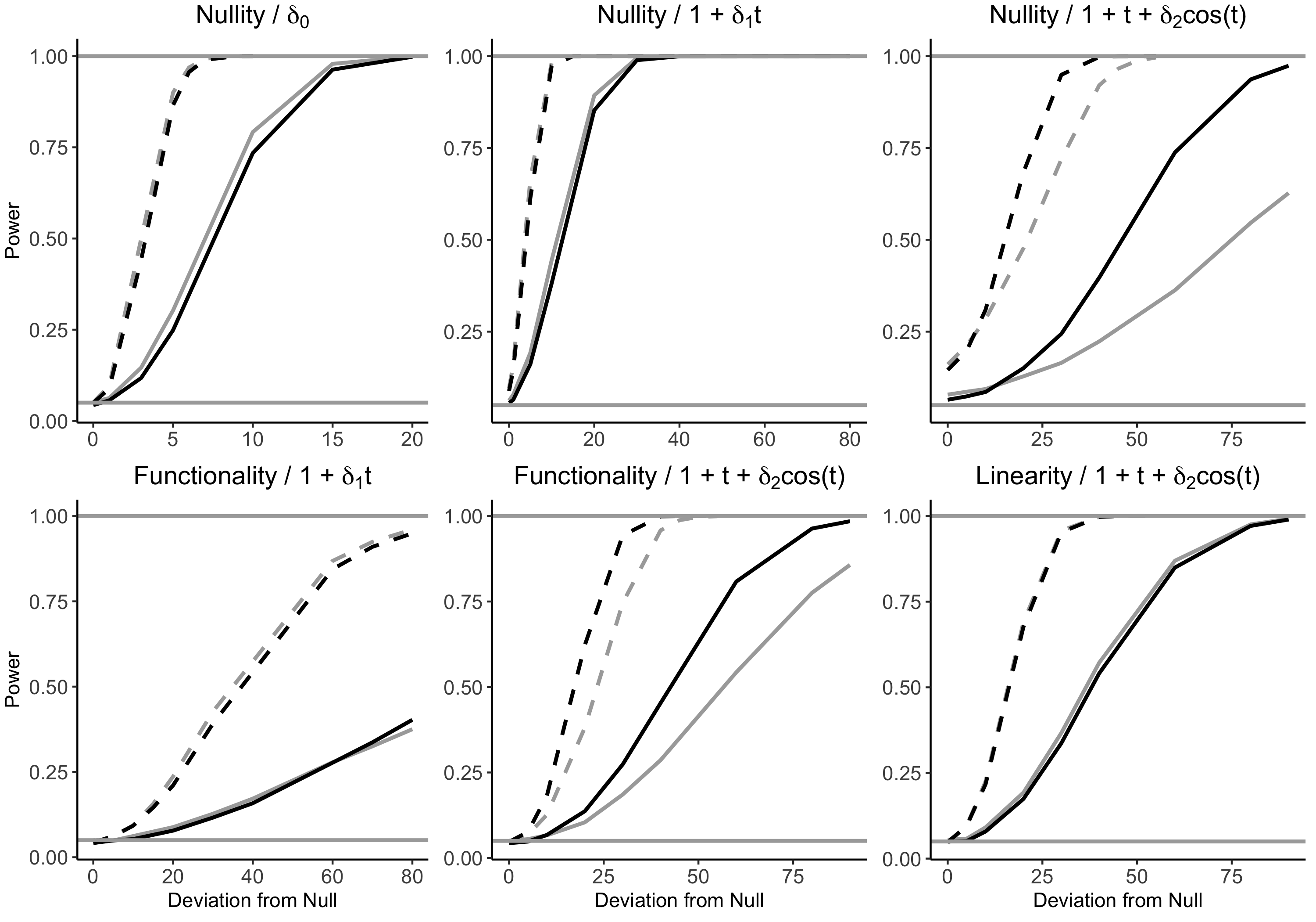
Figure 1: Power for dense binary data at the $\alpha=0.05$ level based on 5000 simulated datasets, by $\beta(t)$ form. Legend: aRLRT (black), aScore (gray), $n=100$ subjects (solid), $n=500$ subjects (dashed).

6 Applications

6.1 Phoneme Classification

We first consider an application to digital speech classification described by Hastie et al. (1995) in the context of penalized discriminant analysis, available as the Phoneme dataset in the fds package (Shang and Hyndman, 2013). Ferraty and Vieu (2003) and Mousavi and Sørenson (2017) found that classification using functional approaches outperformed non-functional methods for curve discrimination. To formally test this observation, we apply the aRLRT and aScore methods to test the form of the smooth coefficient. We focus on the 400 phoneme curves for “aa” (as in the vowel for “dark”) and 400 curves for “ao” (as in the first vowel of “water”). Each curve gives the log-periodogram as a function of frequency measured at a 16-kHz sampling rate, considering only the first 150 frequencies.

Figure 2 shows the data and estimated smooth coefficient from a scalar-on-function linear model with binary responses, where “aa” is assigned value 0 and “ao” is value 1. Visually, the smooth coefficient looks functional and non-linear. The aRLRT method yields highly significant RLRT statistics for the tests for linearity, functionality, and nullity of 112.9, 145.2, and 175.7, respectively, corresponding to $p$-values $<0.001$. Similarly, the aScore method yields highly significant statistics of 10406.6, 8755.5, and 1479.6, respectively, corresponding to $p$-values $<0.001$. Both methods indicate that the smooth coefficient has a non-linear functional form.

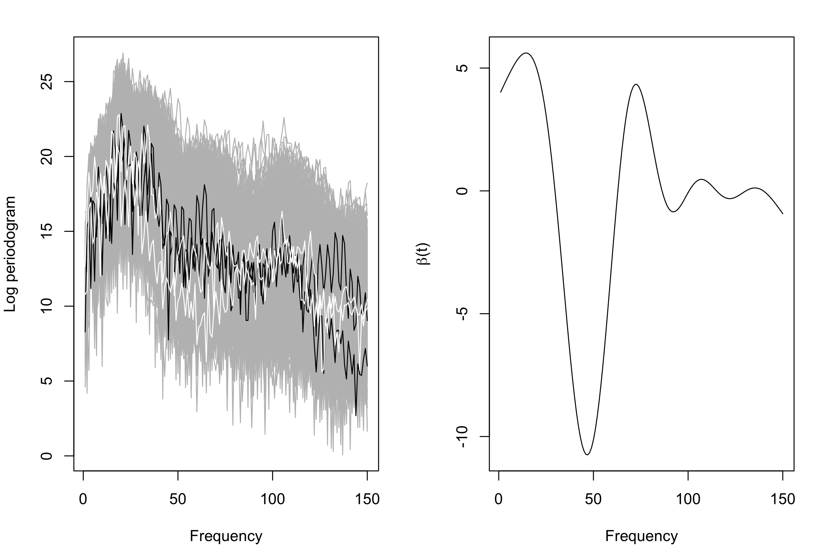
Figure 2: (Left) Phoneme curves with two example “aa” (black) and “ao” (white) highlighted curves. (Right) Estimated coefficient function.

6.2 Identifying Multiple Sclerosis Patients using Diffusion Tensor Imaging

We now consider the motivating example of identifying MS patients using DTI of intracranial white matter microstructure. We focus on the complete baseline fractional anisotropy tract profiles for the (a) corpus callosum (CCA), observed at 93 points for 42 healthy and 99 MS patients, and (b) right corticospinal tract (RCST), observed at 57 points for 26 healthy and 66 MS patients, shown in Figure 3. The CCA connects the right and left hemispheres of the brain and is associated with cognitive function, while the RCST connects to the spinal cord and is associated with motor function. We apply the aRLRT and aScore methods to determine the form of the smooth coefficient in scalar-on-function linear models.

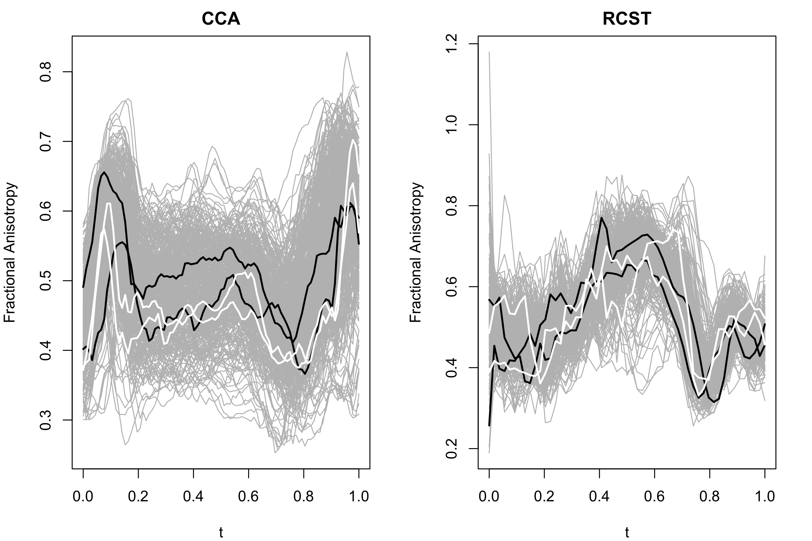
Figure 3: Baseline diffusion tensor imaging tracts for the corpus callosum (CCA) and right corticospinal tract (RCST) for healthy (black) and multiple sclerosis (white) patients.

Table 2 reports results for the aRLRT and aScore methods. While both methods indicate that CCA tracts have a significant non-zero relationship while RCST tracts are unrelated to MS, the simulation study showed that both methods could have low power for binary data with few subjects and weak signal, as in these datasets. In the next section, we consider a power analysis of the CCA data to determine if the methods are underpowered for this application.

Table 2: Testing results for the diffusion tensor imaging (DTI) dataset using the aRLRT and aScore methods.

		aRLRT			aScore
		Linearity	Functionality	Nullity	Linearity	Functionality	Nullity
CCA	statistic	0.829	0.658	24.381	0.205	0.022	0.058
	$p$-value	0.094	0.126	$<$0.001	0.120	0.176	$<$0.001
RCST	statistic	0.647	0.786	1.030	0.298	0.024	0.002
	$p$-value	0.111	0.119	0.108	0.094	0.122	0.159

6.2.1 Power Analysis

Simulated datasets are generated based on the baseline CCA scans of both healthy and MS patients using the estimated $\mu(t)$, $\lambda_{k}$, $\sigma^{2}_{e}$, and $K_{x}=31$, as estimated by AIC, as done in the simulation study in Section 5. We set the smooth coefficient as $\beta(t)=\delta\hat{\beta}(t)$, where $\delta$ controls the magnitude of $\beta(t)$ and $\hat{\beta}(t)$ is the estimated smooth coefficient from the test for linearity (Figure 4, top left panel). Note that $\delta=0$ is the null hypothesis for all three hypotheses and $\delta=1$ is the estimated smooth coefficient. The estimated smooth coefficient looks approximately linear or quadratic. Because both the aRLRT and aScore methods may be underpowered for the given sample size, we also consider datasets with double the number of subjects.

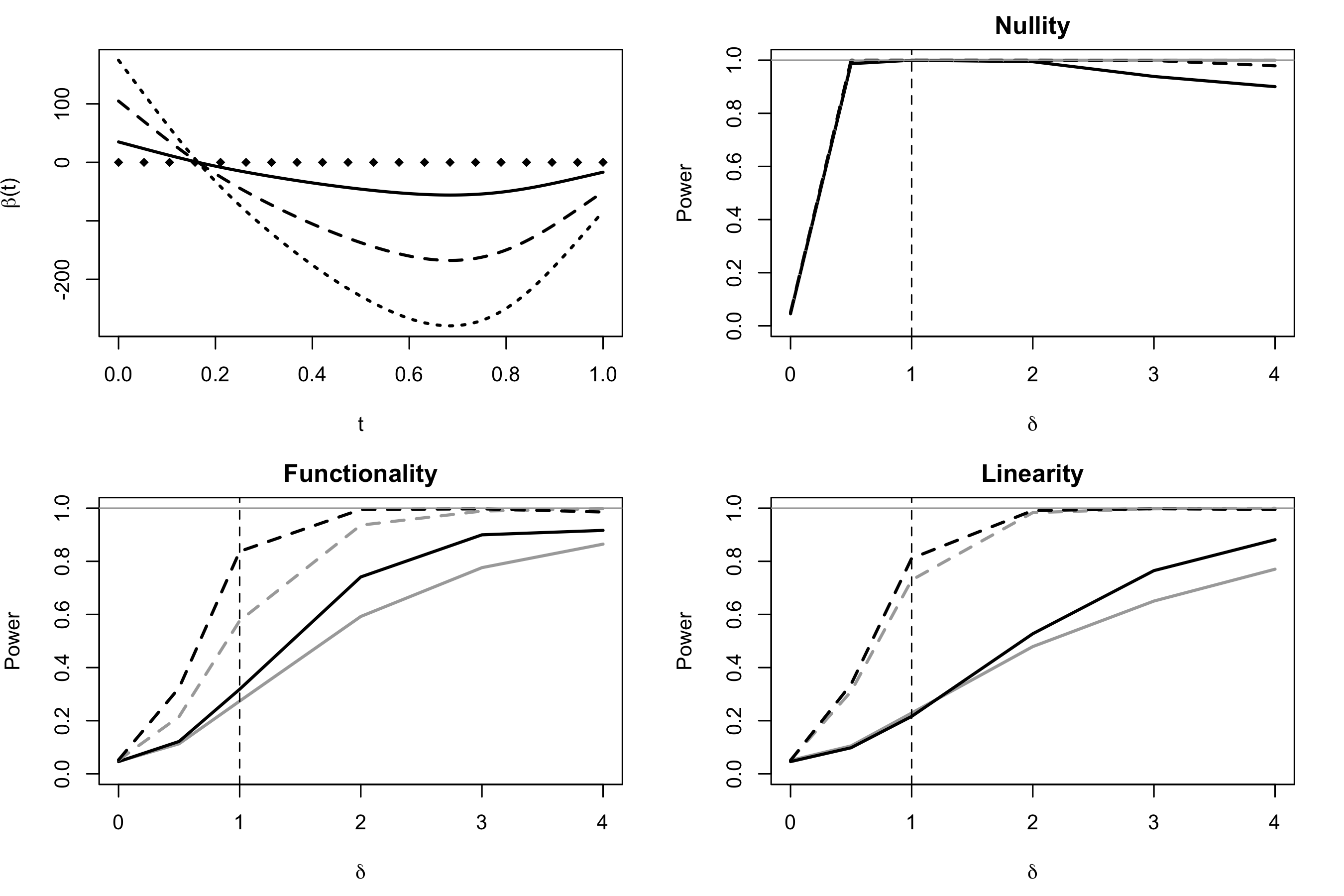
Figure 4: (Top left) Example $\beta(t)=\delta\hat{\beta}(t)$, where $\delta$ controls magnitude and $\hat{\beta}(t)$ is the estimated smooth coefficient. Legend: $\delta=0$ (dotted), $\delta=1$ (solid), $\delta=3$ (long dash), $\delta=5$ (short dash). (Remaining panels) Power for simulated data at the $\alpha=0.05$ level based on 5000 simulated datasets for tests for nullity, functionality, and linearity. Legend: aRLRT (black), aScore (gray), standard dataset (solid), data with $\times 2$ subjects (dashed).

From Figure 4 it is clear that while only the test for nullity has high power for the true sample size, doubling the number of subjects is sufficient to achieve $>80$% power for the aRLRT. This analysis also shows that for small sample sizes, power can decrease even when deviation from the null increases due to instability in the model estimates. Although both methods are likely underpowered for the true dataset, this power analysis suggests that the coefficient may be functional and non-linear. This indicates a non-linear relationship between fractional anisotropy and MS disease status.

7 Conclusion

We propose an approximate restricted likelihood ratio test framework for the smooth coefficient in scalar-on-function linear models with generalized responses. This test can be used compare functional and non-functional linear models with responses from any exponential family distribution. Our method performs well compared to several competitors for dense and sparse data from Bernoulli, Poisson, Binomial, and Normal distributions. Caution should be taken when estimating and testing models for Bernoulli responses when the estimated probabilities are extreme. We apply our test to classifying phoneme curves and identifying multiple sclerosis patients using diffusion tensor imaging.

SUPPLEMENTARY MATERIAL

Additional Results:

Additional simulation results for sparse data, extended competitor methods, and other exponential family distributions available on request from corresponding author.

R code:

R code for all six methods considered in this paper available on request from corresponding author.

References

- Breslow and Clayton (1993) Breslow, N. E. and D. G. Clayton (1993). Approximate inference in generalized linear mixed models. Journal of the American Statistical Association 88, 9–25.
- Cardot et al. (2003a) Cardot, H., F. Ferraty, A. Mas, and P. Sarda (2003a). Spline estimators for the functional linear model. Statistica Sinica 13, 571–591.
- Cardot et al. (2003b) Cardot, H., F. Ferraty, A. Mas, and P. Sarda (2003b). Testing hypotheses in the functional linear model. Scandinavian Journal of Statistics 30, 241–255.
- Chen (2019) Chen, S. T. (2019). glmmVCtest: Testing variance components in generalized linear mixed models. R package version 0.1.0.
- Chen et al. (2019) Chen, S. T., L. Xiao, and A. M. Staicu (2019). An approximate restricted likelihood ratio test for variance components in generalized linear mixed models. Manuscript submitted for publication, 1–20.
- Crainiceanu and Ruppert (2004) Crainiceanu, C. M. and D. Ruppert (2004). Likelihood ratio tests in linear mixed models with one variance component. Journal of the Royal Statistical Society 66, 165–185.
- Eilers and Marx (1996) Eilers, P. H. C. and B. D. Marx (1996). Flexible smooth with b-splines and penalties. Statistical Science 2, 89–102.
- Ferraty and Vieu (2003) Ferraty, F. and P. Vieu (2003). Curves discrimination: a nonparametric functional approach. Computational Statistics & Data Analysis 44, 161–173.
- Ferraty and Vieu (2006) Ferraty, F. and P. Vieu (2006). Nonparametric Functional Data Analysis. New York: Springer.
- Gertheiss et al. (2013) Gertheiss, J., J. Goldsmith, C. M. Crainiceanu, and S. Greven (2013). Longitudinal scalar-on-functions regression with application to tractography data. Biostatistics 14, 447–461.
- Goldsmith et al. (2011) Goldsmith, J., C. M. Crainiceanu, B. Caffo, and D. Reich (2011). Penalized functional regression analysis of white-matter tract profiles in multiple sclerosis. Neuroimage 57, 431–439.
- Goldsmith et al. (2012) Goldsmith, J., C. M. Crainiceanu, B. Caffo, and D. Reich (2012). Longitudinal penalized functional regression for cognitive outcomes on neuronal tract measurements. Applied Statistics 61, 453–469.
- Goldsmith et al. (2018) Goldsmith, J., F. Scheipl, L. Huang, J. Wrobel, J. Gellar, J. Harezlak, M. W. McLean, B. Swihart, L. Xiao, C. Crainiceanu, and P. T. Reiss (2018). refund: Regression with Functional Data. R package version 0.1-17.
- Kong et al. (2016) Kong, D., A. M. Staicu, and A. Maity (2016). Classical testing in functional linear models. Journal of Nonparametric Statistics 28, 813–838.
- Li et al. (2013) Li, Y., N. Wang, and R. J. Carroll (2013). Selecting the number of principal components in functional data. Journal of the American Statistical Association 108, 1284–1294.
- Lin (1997) Lin, X. (1997). Variance component testing in generalised linear models with random effects. Biometrika 84, 309–326.
- McLean et al. (2015) McLean, M. W., G. Hooker, and D. Ruppert (2015). Restricted likelihood ratio tests for linearity in scalar-on-function regression. Statistical Computing 25, 997–1008.
- Molenberghs and Verbeke (2007) Molenberghs, G. and G. Verbeke (2007). Likelihood ratio, score, and wald tests in a constrained parameter space. The American Statistician 61, 22–27.
- Morris (2015) Morris, J. S. (2015). Functional regression. Annual Review of Statistics and Its Application 2, 321–359.
- Mousavi and Sørenson (2017) Mousavi, S. N. and H. Sørenson (2017). Multinomial functional regression with wavelets and lasso penalization. Econometrics and Statistics 1, 150–166.
- Pinheiro and Bates (2000) Pinheiro, J. C. and D. B. Bates (2000). Mixed-Effects Models in S and S-PLUS. New York: Springer.
- Ramsay and Silverman (2002) Ramsay, J. O. and B. W. Silverman (2002). Applied Functional Data Analysis. New York: Springer.
- Ramsay and Silverman (2005) Ramsay, J. O. and B. W. Silverman (2005). Functional Data Analysis. New York: Springer.
- Reich et al. (2010) Reich, D. S., A. Ozturk, P. A. Calabresi, and S. Mori (2010). Automated vs. conventional tractography in multiple sclerosis: Variability and correlation with disability. Neuroimage 49, 3047–3056.
- Schall (1991) Schall, R. (1991). Estimation in generalized linear mixed models with random effects. Biometrika 78(4), 719–727.
- Scheipl and Greven (2016) Scheipl, F. and S. Greven (2016). Identifiability in penalized function-on-function regression models. Electronic Journal of Statistics 10, 495–526.
- Scheipl et al. (2008) Scheipl, F., S. Greven, and H. Küechenhoff (2008). Size and power of tests for a zero random effect variance or polynomial regression in additive and linear mixed models. Computational Statistics & Data Analysis 52(7), 3283–3299.
- Self and Liang (1987) Self, S. G. and K.-Y. Liang (1987). Asymptotic properties of maximum likelihood estimators and likelihood ratio tests under nonstandard conditions. Journal of the American Statistical Association 82, 605–610.
- Shang and Hyndman (2013) Shang, H. L. and R. J. Hyndman (2013). fds: Functional data sets. R package version 1.7.
- Swihart et al. (2014) Swihart, B. J., J. Goldsmith, and C. M. Crainiceanu (2014). Restricted likelihood ratio tests for functional effects in the functional linear model. Technometrics 56, 483–493.
- vanescu et al. (2015) vanescu, A. E., A. M. Staicu, F. Scheipl, and S. Greven (2015). Penalized function-on-function regression. Computational Statistics 30, 539–568.
- Wolfinger and O’conell (1993) Wolfinger, R. and M. O’conell (1993). Generalized linear mixed models: a pseudo-likelihood approach. Journal of statistical computation and simulation 48, 233–243.
- Xiao et al. (2016) Xiao, L., D. Ruppert, V. Zipunnikov, and C. M. Crainiceanu (2016). Fast covariance function estimation for high-dimensional functional data. Statistics and Computing 26, 409–421.
- Yao et al. (2005) Yao, F., H. G. Müller, and W. J. L. (2005). Functional data analysis for sparse longitudinal data. Journal of the American Statistical Association 100, 577–590.
- Zhang and Lin (2003) Zhang, D. and X. Lin (2003). Hypothesis testing in semiparametric additive mixed models. Biostatistics 4, 57–74.
- Zhu et al. (2010) Zhu, H., M. Styner, N. Tang, Z. Liu, and J. H. Gilmore (2010). Frats: Functional regression analysis of dti tract statistics. IEEE Trans Med Imaging 29, 1039–1049.