Resource-efficient topological fault-tolerant quantum computation with hybrid entanglement of light

Abstract

We propose an all-linear-optical scheme to ballistically generate a cluster state for measurement-based topological fault-tolerant quantum computation using hybrid photonic qubits entangled in a continuous-discrete domain. Availability of near-deterministic Bell-state measurements on hybrid qubits is exploited for the purpose. In the presence of photon losses, we show that our scheme leads to a significant enhancement in both tolerable photon-loss rate and resource overheads. More specifically, we report a photon-loss threshold of $\sim 3.3\times 10^{-3}$, which is higher than those of known optical schemes under a reasonable error model. Furthermore, resource overheads to achieve logical error rate of $10^{-6}(10^{-15})$ is estimated to be $\sim 8.5\times 10^{5}(1.7\times 10^{7})$ which is significantly less by multiple orders of magnitude compared to other reported values in the literature.

Errors during quantum information processing are unavoidable, and they are a major obstacle against practical implementations of quantum computation (QC) Nielsen and Chuang (2010). Quantum error correction (QEC) Lidar and Brun  (eds.) permits scalable QC with faulty qubits and gates provided the noise is below a certain threshold. The noise threshold is determined by the details of the implementing scheme and the noise model.

Measurement-based topological fault-tolerant (FT) QC Raussendorf et al. (2006) on a cluster state provides a high error threshold of $0.75\%$ against computational errors Raussendorf et al. (2007); Raussendorf and Harrington (2007). Additionally, it can tolerate qubit losses Barrett and Stace (2010); Whiteside and Fowler (2014) and missing edges Li et al. (2010); thus, it would be suitable for practical large-scale QC. However, there is a trade-off between the tolerable computational error rate, and the tolerable level of qubit losses and missing edges. A cluster state $\left|\mathcal{C}\right\rangle$, over a collection of qubits $\mathcal{C}$, is the state stabilized by operators $X_{a}\bigotimes_{b\in\rm{nh}(a)}Z_{b}$, where $a,b\in\mathcal{C}$, $Z_{i}$ and $X_{i}$ are the Pauli operators on the $i$th qubit, and nh(a) represents the adjacent neighborhood of qubit $a\in\mathcal{C}$ Briegel and Raussendorf (2001). It has the form: $\left|\mathcal{C}\right\rangle=\prod_{b\in\rm{nh}(a)}\textrm{CZ}_{a,b}\left|+\right\rangle_{a}\left|+\right\rangle_{b},~{}\forall a\in\mathcal{C}$, where CZ is the controlled-Z gate, $\left|\pm\right\rangle=(\left|0\right\rangle\pm\left|1\right\rangle)/\sqrt{2}$, and $\{\left|0\right\rangle,\left|1\right\rangle\}$ are eigenstates of $Z$. Here, we consider the Raussendorf cluster state $\left|\mathcal{C}_{\mathcal{L}}\right\rangle$ Raussendorf et al. (2006) on a cubic lattice $\mathcal{L}$ with qubits mounted on its faces and edges.

The linear optical platform has the advantage of quick gate operations compared to their decoherence time Ralph and Pryde (2010). Unfortunately, schemes based on discrete variables (DV) like photon polarizations suffer from the drawback that the entangling operations (EOs), typically implemented by Bell-state measurements, are nondeterministic Browne and Rudolph (2005). This leaves the edges corresponding to all failed EOs missing, and beyond a certain failure rate the cluster state cannot support QC. References Nielsen (2004); Dawson et al. (2006); Li et al. (2010); Fujii and Tokunaga (2010); Herrera-Martí et al. (2010) tackle this shortcoming with a repeat-until-success strategy. However, this strategy incurs heavy resource overheads in terms of both qubits and EO trials, and the overheads grow exponentially as the success rate of EO falls Li et al. (2010). Moreover, conditioned on the outcome of the EO, all other redundant qubits must be removed via measurements Fujii and Tokunaga (2010) which would add to undesirable resource overheads. These schemes also require active switching to select successful outcomes of EOs and feed them to the next stage, which is known to have an adverse effect on the photon-loss threshold for FTQC Li et al. (2015). DV-based optical EOs have a success rate of 50% that can be further boosted with additional resources like single photons Ewert and van Loock (2014), Bell states Grice (2011) and the squeezing operation Zaidi and van Loock (2013). Reference Gimeno-Segovia et al. (2015) uses EOs with boosted success rate of 75% to build cluster states. This can be further enhanced by allotting more resources. Coherent-state qubits, composed of coherent states $|\pm\alpha\rangle$ of amplitudes $\pm\alpha$, enable one to perform nearly deterministic Bell-state measurements and universal QC using linear optics Jeong and Kim (2002); Ralph et al. (2003), while this approach is generally more vulnerable to losses Lund et al. (2008); Ralph and Pryde (2010). Along this line, a scheme to generate cluster states for topological QC was suggested, but the value of $\alpha$ required to build a cluster state of sufficiently high fidelity is unrealistically large as $\alpha>20$ Myers and Ralph (2011). A hybrid qubit using both DV and continuous-variable (CV) states of light, i.e., polarized single photons and coherent states was introduced to take advantages of both the approaches Lee and Jeong (2013).

We propose an all-linear-optical measurement-based FT hybrid topological QC (HTQC) scheme on $\left|\mathcal{C}_{\mathcal{L}}\right\rangle$ of hybrid qubits. The logical basis for a hybrid qubit is defined as $\{\left|\alpha\right\rangle\left|\textsc{h}\right\rangle\equiv\left|0_{\rm L}\right\rangle,\left|-\alpha\right\rangle\left|\textsc{v}\right\rangle\equiv\left|1_{\rm L}\right\rangle\}$, where $\left|\textsc{h}\right\rangle$ and $\left|\textsc{v}\right\rangle$ are single-photon states with horizontal and vertical polarizations in the $Z$ direction. The issues with indeterminism of EOs on DVs Dawson et al. (2006); Li et al. (2010); Fujii and Tokunaga (2010); Herrera-Martí et al. (2010) and poor fidelity of the cluster states with CVs Myers and Ralph (2011) are then overcome. Crucial to our scheme is a near-deterministic hybrid Bell-state measurement (HBSM) on hybrid qubits using two photon number parity detectors (PNPDs) and two on-off photodetectors (PDs), which is distinct from the previous version that requires two additional PDs to complete a teleportation protocol Lee and Jeong (2013). We only need HBSMs acting on three-hybrid-qubit cluster states to generate $\left|\mathcal{C}_{\mathcal{L}}\right\rangle$ without any active switching and feed-forward. The outcomes of HBSMs are noted to interpret the measurement results during QEC and QC. In this sense, our scheme is ballistic in nature. Both CV and DV modes of hybrid qubits support the HBSMs to build $\left|\mathcal{C}_{\mathcal{L}}\right\rangle$, while only DV modes suffice for QEC and QC. This means that only on-off PDs for DV modes are required once $\left|\mathcal{C}_{\mathcal{L}}\right\rangle$ is generated. In addition, photon loss is ubiquitous Ralph and Pryde (2010) that causes dephasing such as in Lee and Jeong (2013); Lund et al. (2008); Lee et al. (2015). We analyze the performance of our scheme against photon losses and compare it with the known all-optical schemes.

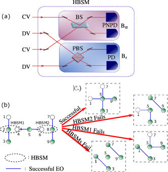
Figure 1: (a) $\mathrm{B}_{\alpha}\,$ acts on CV modes and fails when neither of the two PNPDs click. The failure rate of a $\mathrm{B}_{\alpha}\,$ on the hybrid qubits is $\mathrm{e}^{\mbox{\footnotesize$-2\alpha^{2}$}}$. $\rm{B}_{\rm{s}}$ acts on DV modes and is successful with probability $1/2$ only when both the PDs click. (b) The three-hybrid-qubit cluster with one unfilled circle represents $\left|\mathcal{C}_{3}\right\rangle$, while that with two represents $\left|\mathcal{C}_{3^{\prime}}\right\rangle$ in Eq. (B). An unfilled circle means a difference by a Hadamard transform from the original three-qubit cluster (see Appendix B). Success of both HBSMs creates a star cluster $\left|\mathcal{C}_{\ast}\right\rangle$ and other cases lead to distorted star clusters as shown.

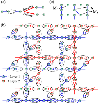
Figure 2: (a) When connecting $\left|\mathcal{C}_{\ast}\right\rangle$’s, a successful HBSM creates an edge between hybrid qubits whereas a failed HBSM leaves the edge missing. (b) 3D illustration of building two layers of $\left|\mathcal{C}_{\mathcal{L}}\right\rangle$ for practical HTQC with $\left|\mathcal{C}_{\ast}\right\rangle$’s and HBSMs to connect them. (c) A diagonal edge is created due to failure of an HBSM corresponding to $\left|\mathcal{C}_{\ast}\right\rangle$ and a missing edge is due to failure of an HBSM while connecting them. A single layer of $\left|\mathcal{C}_{\mathcal{L}}\right\rangle$ is shown for convenience, and ${\rm M_{z}}$ is measurement in Z-basis.

Physical platform for $\left|\mathcal{C}_{\mathcal{L}}\right\rangle$.— To ballistically build a $\left|\mathcal{C}_{\mathcal{L}}\right\rangle$, we begin with hybrid qubits, in the form $(\left|\textsc{h}\right\rangle|\alpha\rangle+\left|\textsc{v}\right\rangle|-\alpha\rangle)/\sqrt{2}=(|0_{\rm L}\rangle+|1_{\rm L}\rangle)/\sqrt{2}\equiv|+_{\rm L}\rangle$, as raw resources of our scheme. In fact, this type of hybrid qubits and with slight variant forms (with the vacuum and single photon instead of $|H\rangle$ and $|V\rangle$) were generated in recent experiments Sychev et al. (2018); Jeong et al. (2014); Morin et al. (2014), which can also be used for QC in the same way as in Lee and Jeong (2013) even with higher fidelities and success probabilities of teleportation Kim et al. (2016). A hybrid qubit can also be generated using a Bell-type photon pair, a coherent-state superposition, linear optical elements and four PDs Kwon and Jeong (2015).

The HBSM introduced in this Letter consists of two types of measurements, $\mathrm{B}_{\alpha}\,$ and $\rm B_{s}$, acting on CV and DV modes, respectively. A Bell-state measurement for coherent-state qubits Jeong et al. (2001), $\mathrm{B}_{\alpha}\,$, comprises of a beam splitter (BS) and two PNPDs, whereas $\rm B_{s}$ has a polarizing BS (PBS) and two PDs as shown in Fig. 1(a). The failure rate for an HBSM turns out to be $p_{f}=\mathrm{e}^{\mbox{\footnotesize$-2\alpha^{2}$}}\!\!/2$ (see Appendix A and also Lee and Jeong (2013)) that rapidly approaches zero with growing $\alpha$. The first and only nondeterministic step of our protocol is to prepare two kinds of three-hybrid-qubit cluster states,

$$\left|\mathcal{C}_{3}\right\rangle_{abc} = \frac{1}{2}\big{(}\left|0_{\rm L}\right\rangle_{a}\left|0_{\rm L}\right\rangle_{b}\left|0_{\rm L}\right\rangle_{c}+\left|0_{\rm L}\right\rangle_{a}\left|0_{\rm L}\right\rangle_{b}\left|1_{\rm L}\right\rangle_{c}$$

$$+\left|1_{\rm L}\right\rangle_{a}\left|1_{\rm L}\right\rangle_{b}\left|0_{\rm L}\right\rangle_{c}-\left|1_{\rm L}\right\rangle_{a}\left|1_{\rm L}\right\rangle_{b}\left|1_{\rm L}\right\rangle_{c}\big{)},$$

$$\left|\mathcal{C}_{3^{\prime}}\right\rangle_{abc} = \frac{1}{\sqrt{2}}\big{(}\left|0_{\rm L}\right\rangle_{a}\left|0_{\rm L}\right\rangle_{b}\left|0_{\rm L}\right\rangle_{c}+\left|1_{\rm L}\right\rangle_{a}\left|1_{\rm L}\right\rangle_{b}\left|1_{\rm L}\right\rangle_{c}\big{)}~{}$$ (1)

using four hybrid qubits, two $\rm B_{\alpha}$’s and a $\rm B_{I}$ as detailed in Appendix B . (Here, $\rm B_{I}$ is a type-I fusion gate using two PBSs, two PDs and a $\pi/2$-rotator, of which the success probability is 1/2. See Appendix A for details.) As shown in Fig. 1(b), an HBSM is performed on modes $2$ and $4$ of $\left|\mathcal{C}_{3}\right\rangle_{123}$ and $\left|\mathcal{C}_{3^{\prime}}\right\rangle_{456}$, and the other HBSM is performed similarly between $\left|\mathcal{C}_{3^{\prime}}\right\rangle_{456}$ and $\left|\mathcal{C}_{3}\right\rangle_{789}$, which produces a star cluster, $\left|\mathcal{C}_{\ast}\right\rangle$, with a high success probability. Simultaneously, the star clusters are connected using HBSMs to form layers of $\left|\mathcal{C}_{\mathcal{L}}\right\rangle$ as depicted in Fig. 2(b). As the third dimension of $\left|\mathcal{C}_{\mathcal{L}}\right\rangle$ is time simulated, in practice only two physical layers suffice for QC Raussendorf et al. (2007).

Notably, different outcomes of HBSMs and failures during this process can be compensated during QEC as explained below. As HBSMs have four possible outcomes from $\mathrm{B}_{\alpha}\,$, the built cluster state is equivalent to $\left|\mathcal{C}_{\mathcal{L}}\right\rangle$ up to local Pauli operations. This can be compensated by accordingly making bit flips to the measurement outcomes during QEC. This is achieved by classical processing and no additional quantum resources are required. As shown in Fig. 1(b), failure(s) of HBSMs result(s) in a deformed star cluster with diagonal edge(s) instead of four proper edges stretching from the central qubit. The final cluster state $\left|\mathcal{C}_{\mathcal{L}}\right\rangle$ inherits these diagonal edges as shown in Fig. 2(c) with a disturbed stabilizer structure. However, failures of HBSMs are heralded, which reveals the locations of such diagonal edges. These diagonal edges can be removed by adaptively measuring the hybrid qubits in $Z$-basis (${\rm M}_{Z}$), as shown in Fig. 2(c), restoring back the stabilizer structure of $\left|\mathcal{C}_{\mathcal{L}}\right\rangle$. Failure of HBSMs for connecting $\left|\mathcal{C}_{*}\right\rangle$’s simply leaves the edges missing as shown in Fig. 2(a) without distorting the stabilizer structure.

Noise model.— Let $\eta$ be the photon-loss rate due to imperfect sources and detectors, absorptive optical components and storages. In HTQC, the effect of photon loss is threefold (see Appendix C and also Lee and Jeong (2013)) that (i) causes dephasing of hybrid qubits i.e., phase-flip errors $Z$, a form of computational error, with rate $p_{Z}=[1-(1-\eta)\,\mathrm{e}^{\mbox{\footnotesize$-2\eta\alpha^{2}$}}]/2$, (ii) lowers the success rate of HBSM and (iii) makes hybrid qubits leak out of the logical basis. Quantitatively, $p_{f}$ increases to $(1+\eta)\mathrm{e}^{\mbox{\footnotesize$-2\alpha^{\prime 2}$}}/2$, where $\alpha^{\prime}=\sqrt{1-\eta}\alpha$. Thus, for a given $\eta$ and growing $\alpha$ we face a trade-off between the desirable success rate of HBSM and the detrimental dephasing rate $p_{Z}$.

Further, like the type-II fusion gate in Varnava et al. (2008), ${\rm B_{s}}$ does not introduce computational errors during photon loss. However, the action of $\mathrm{B}_{\alpha}\,$ on the lossy hybrid qubits introduces additional dephasing as shown in as shown in the Appendix C.1. To clarify, like DV schemes Herrera-Martí et al. (2010), photon loss does not imply hybrid-qubit loss. In many FTQC schemes $\eta$ has a typical operational value of $\sim 10^{-3}$ (on the higher side) Lee et al. (2015); Dawson et al. (2006); Hayes et al. (2010); Cho (2007), i.e., $\eta\ll 1$. The probability of hybrid-qubit loss due to photon loss, $\eta\mathrm{e}^{\mbox{\footnotesize$-\alpha^{\prime 2}$}}$ (the overlap between a lossy hybrid qubit and the vacuum), is then very small compared to $p_{f}$ and negligible to HTQC.

Measurement-based HTQC.— Once the faulty cluster state is built with missing and diagonal edges, and phase-flip errors on the constituent hybrid qubits, measurement-based HTQC is performed by making sequential single-qubit measurements in $X$ and $Z$ bases. A few chosen ones are measured in $Z$-basis to create defects, and the rest are measured in X-basis for error syndromes during QEC and for effecting the Clifford gates on the logical states of $\left|\mathcal{C}_{\mathcal{L}}\right\rangle$. For Magic state distillation, measurements are made in $(X\pm Y)/\sqrt{2}$ basis Raussendorf et al. (2006); Raussendorf and Harrington (2007); Raussendorf et al. (2007). All these measurements are accomplished by measuring only polarizations of DV modes in the respective basis. These measurement outcomes should be interpreted with respect to the recorded HBSM outcomes as mentioned earlier.

Simulations.— Simulation of topological QEC is performed using AUTOTUNE Fowler et al. (2012) (see Appendix D for a brief description). Only the central hybrid qubit of $\left|\mathcal{C}_{\ast}\right\rangle$ remains in the cluster and the rest are utilized by HBSMs. The $\left|\mathcal{C}_{\ast}\right\rangle$’s are arranged as shown in Fig. 2. Next, all hybrid qubits are subjected to dephasing of rate $p_{Z}$ following which EOs are performed using HBSMs. The action of $\mathrm{B}_{\alpha}\,$ in HBSM dephases the adjacent remaining hybrid qubits, which can be modeled as applying $\{Z\otimes I,I\otimes Z\}$ with rate $p_{Z}$. The technical details of the action of $\mathrm{B}_{\alpha}\,$ under photon loss are presented in the Appendix C.1. This concludes the simulation of building noisy $\left|\mathcal{C}_{\mathcal{L}}\right\rangle$. Further, the hybrid qubits waiting to undergo measurements as a part of QEC attract dephasing, and rate $p_{Z}$ again is assigned. During QEC, $X$-measurement outcomes used for syndrome extraction could be erroneous. This error too is assigned rate $p_{Z}$. Due to photon losses, the hybrid qubits leak out of the logical basis failing the measurements on DV modes. This leakage is also assigned $p_{Z}$, which only overestimates $\eta$.

One missing edge due to failed HBSMs can be mapped to two missing hybrid qubits Li et al. (2010). Improving on this, by adaptively performing ${\rm M}_{Z}$ (Fig. 2(c)) on one of the hybrid qubits associated with a missing edge, this edge can be modeled with a missing qubit Auger et al. (2018). Then, QEC is carried out as in the case of missing qubits Barrett and Stace (2010). In constructing $\left|\mathcal{C}_{\mathcal{L}}\right\rangle$, an equal number of HBSMs are required for building $\left|\mathcal{C}_{\ast}\right\rangle$ and for connecting them. A failure of an HBSM during the former process corresponds to two hybrid-qubit losses, and the latter case to one (Fig. 2(c)). Therefore, on average 1.5 hybrid qubits per HBSM failure are lost. Percolation threshold for $\left|\mathcal{C}_{\mathcal{L}}\right\rangle$ is $0.249$ fraction of missing qubits Barrett and Stace (2010); Lorenz and Ziff (1998); Pant et al. (2019), which corresponds to $\alpha\approx 0.7425$ (when no computational error is tolerated, i.e., $\eta=0$), the critical value of $\alpha$ below which HTQC becomes impossible.

Results.— The logical error rate $p_{\rm L}$ (failure rate of topological QEC Raussendorf et al. (2007)) was determined against various values of $p_{Z}$ for $\left|\mathcal{C}_{\mathcal{L}}\right\rangle$ of code distances $d=3,5,7$. This was repeated for various values of $p_{f}$ which correspond to different values of $\alpha$. Figure 3(a) shows the simulation results for $\alpha_{\rm opt}=1.247$ in which the intersection point of the curves corresponds to the threshold dephasing rate $p_{Z,\rm th}$. The photon-loss threshold $\eta_{\rm th}$ is determined using the expression for $p_{Z}$.

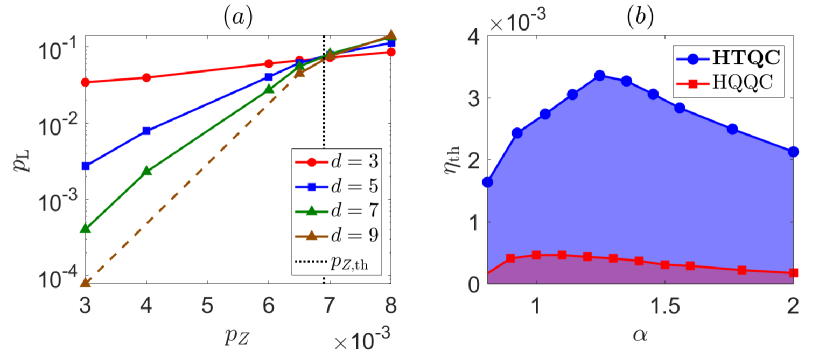
Figure 3: (a) Logical error rate $p_{\rm L}$ is plotted against the dephasing rate $p_{Z}$ for coherent-state amplitude $\alpha_{\rm opt}=1.247$ and code distances $d=3,5,7$. The intersecting point of these curves corresponds to the threshold dephasing rate $p_{Z,\rm th}$. (b) The tolerable photon-loss rate $\eta_{\rm{th}}$ is plotted against coherent-state amplitude $\alpha$. The behavior of the curve is due to the trade-off between the success rate of HBSM and dephasing rate $p_{Z}$ with growing $\alpha$. As we increase $\alpha$, both the success rate and $p_{Z}$ increase; but the former dominates and leads to an increase in $\eta_{\rm th}$. When $\alpha>1.247$, $p_{Z}$ dominates and causes $\eta_{\rm th}$ to decrease. Compared to the non-topoligical HQQC Lee and Jeong (2013), HTQC has an order of higher value for $\eta_{\rm th}$.

Figure 3(b) shows the behavior of $\eta_{\rm th}$ with $\alpha$. Owing to the trade-off between $p_{f}$ and $p_{Z}$, the optimal value for HTQC is $\alpha_{\rm opt}\approx 1.25$ which corresponds to $\eta_{\rm th}\approx 3.3\times 10^{-3}$ and $p_{Z,\rm th}\approx 6.9\times 10^{-3}$. The value of $\eta_{\rm th}$ for $0.8\leq\alpha\leq 2$ is on the order of $10^{-3}$, which is an order greater than the non-topological hybrid-qubit-based QC (HQQC) Lee and Jeong (2013) and coherent state QC (CSQC) Lund et al. (2008). HTQC also outperforms the DV based topological photonic QC (TPQC) with $\eta_{\rm th}\approx 5.5\times 10^{-4}$ Herrera-Martí et al. (2010). Multi-photon qubit QC (MQQC) Lee et al. (2015), parity state linear optical QC (PLOQC) Hayes et al. (2010) and error-detecting quantum state transfer based QC (EDQC) Cho (2007) provide $\eta_{\rm th}$’s which are less than HTQC but of the same order as illustrated in Fig. 4(a). In addition, $\eta$ and the computational error rates are independent in Hayes et al. (2010); Dawson et al. (2006); Cho (2007), while these two quantities are related in our scheme and Refs. Lee and Jeong (2013); Lund et al. (2008); Lee et al. (2015). Also in the former schemes the computational error is dephasing in nature, and in the latter schemes it is depolarizing. In fact, $\eta_{\rm th}$’s claimed by optical cluster-state QC (OCQC) Dawson et al. (2006), PLOQC, EDQC and TPQC are valid only for zero computational error. This is unrealistic because photon losses typically cause computational errors. For the computational error rate as low as $8\times 10^{-5}$, $\eta_{\rm th}=0$ in OCQC. Thus, for non-zero computational errors, HTQC also outperforms OCQC due to its topological nature of QEC.

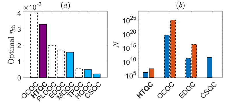
Figure 4: (a) Optimal photon-loss threshold $\eta_{\rm th}$ for various QC schemes. It should be noted that $\eta_{\rm{th}}$’s of OCQC, PLOQC, EDQC and TPQC (dashed borders) are valid only for zero computational error, which is physically unachievable. Other schemes evaluate optimal $\eta_{\rm th}$ at nonzero computational errors naturally related to $\eta$. (b) Resource overhead $N$ to achieve logical error rate $p_{\rm L}\sim 10^{-6}({\rm blue~{}shorter~{}bars})$ and $p_{\rm L}\sim 10^{-15}({\rm orange~{}taller~{}bars})$ in terms of the average numbers of hybrid qubits (HTQC), entangled photon pairs (OCQC and EDQC), coherent-state superpositions (CSQC) from our analysis and published data in Dawson et al. (2006); Cho (2007); Lund et al. (2008). For CSQC data only for $p_{\rm L}\sim 10^{-6}$ is available Lund et al. (2008). Obviously, HTQC is practically favorable for large scale QC both in terms of $\eta_{\rm th}$ and $N$. See Appendix E for more details of comparisons.

To estimate the resource overhead per gate operation, we count the average number of hybrid qubits $N$ required to build $\left|\mathcal{C}_{\mathcal{L}}\right\rangle$ of a sufficiently large side length $l$, where the desired value of $l$ depends on the target $p_{\rm L}$. The length $l$ is determined such that $\left|\mathcal{C}_{\mathcal{L}}\right\rangle$ can accommodate defects of circumference $d$ which are separated by distance $d$ Whiteside and Fowler (2014). For this, the length of sides must be at least $l=5d/4$. Extrapolating the suppression of $p_{\rm L}$ with code distance, we determine the value of $d$ required to achieve the target $p_{\rm L}$ using the expression $p_{\rm L}=a^{\prime}/[(a/a^{\prime})^{(d-d_{a^{\prime}})/2}]$ Whiteside and Fowler (2014), where $a$ and $a^{\prime}$ are values of $p_{\rm L}$ corresponding to the second highest and the highest distances, $d_{a}$ and $d_{a^{\prime}}$, chosen for simulation. Once $d$ is determined, $N$ can be estimated as follows. Recall that two $\left|\mathcal{C}_{3}\right\rangle$’s and a $\left|\mathcal{C}_{3^{\prime}}\right\rangle$ are needed to build a $\left|\mathcal{C}_{\ast}\right\rangle$. On average, $8/[(1-\mathrm{e}^{\mbox{\footnotesize$-2\alpha^{\prime 2}$}})^{2}]$ hybrid qubits are needed to create a three-hybrid-qubit cluster ( as shown in Appendix B) and a total of $24/[(1-\mathrm{e}^{\mbox{\footnotesize$-2\alpha^{\prime 2}$}})^{2}]$ hybrid qubits for a $\left|\mathcal{C}_{\ast}\right\rangle$. Each $\left|\mathcal{C}_{\ast}\right\rangle$ corresponds to a single hybird qubit in the $\left|\mathcal{C}_{\mathcal{L}}\right\rangle$ and thus the number of $\left|\mathcal{C}_{\ast}\right\rangle$’s needed is $6l^{3}$. Finally, on average, $1125d^{3}/[4(1-\mathrm{e}^{\mbox{\footnotesize$-2\alpha^{\prime 2}$}})^{2}]$ hybrid qubits are incurred. For the optimal value of $\alpha_{\rm opt}\approx 1.25$, from Fig. 3(a) we have $a\approx 4.4\times 10^{-4}$, $a^{\prime}\approx 7.9\times 10^{-5}$ and $d_{a^{\prime}}=9$; using these in the expression for $p_{\rm L}$ we find that $d\approx 14~{}(38)$ is needed to achieve $p_{\rm L}\sim 10^{-6}~{}(10^{-15})$. This incurs $N\approx 8.5\times 10^{5}~{}(1.7\times 10^{7})$ hybrid qubits.

Comparisons in Fig. 4(b) and in Appendix E show that HTQC incurs resources significantly less than all the other schemes under consideration. As an example, for the case of TPQC, we find $a=0.065$ and $a^{\prime}=0.059$ from Fig. 7(a) of Herrera-Martí et al. (2010), where the figure considers only computational errors. Thus, TPQC under computational errors needs $d=225~{}(621)$ to attain $p_{\rm L}\sim 10^{-6}~{}(10^{-15})$. Since a qubit in TPQC needs $2R+1$ photons on average as resources Herrera-Martí et al. (2010), we obtain $N=(2R+1)\times 6(5d/4)^{3}$ (derived in Appendix E), where $R=7$ for maximum $\eta_{\rm th}$ Herrera-Martí et al. (2010). We then find $N=2\times 10^{9}$ $(4.2\times 10^{10})$ for TPQC, and it must be even larger when qubit losses are considered together with computational errors (see Appendix E for an elaborate discussion).

Discussion.— Our proposal permits the construction of cluster states with very few missing edges that subsequently support QEC and QC only with photon on-off measurements. We simulated its performance and found that our scheme is significantly more efficient than other known schemes in terms of both resource overheads and photon-loss thresholds (Fig. 4), especially when exceedingly small logical error rates are desired for large-scale QC. We have considered measurements only on DV modes of hybrid qubits for QEC. However, measurements on CV modes can also be used, which will significantly reduce leakage errors and improve the photon-loss threshold. The scheme requires hybrid qubits of $\alpha\approx\sqrt{2}\times 1.25$ as raw resource states, which can in principle be generated using available optical sources, linear optics and photodetectors Jeong et al. (2014); Morin et al. (2014); Kwon and Jeong (2015).

One may examine other decoders tailored to take advantage of dephasing noise instead of minimum weight perfect match Fowler (2012), such as in  Tuckett et al. (2018), for improvement of the photon-loss threshold. Different single-qubit noise models Omkar et al. (2013) may be considered to study the performance of HTQC. A sideline task would be in-situ noise characterization using the available syndrome data Omkar et al. (2015a, b, 2016); Fowler et al. (2014). The procedure proposed here to build complex hybrid clusters can also be used to build lattices of other geometries for QC Bombin and Martin-Delgado (2007); Gimeno-Segovia et al. (2015); Zaidi et al. (2015) and other tasks such as communication Azuma et al. (2015).

Appendix A Bell State Measurement on hybrid qubits

The hybrid-Bell state measurement (HBSM) depicted in Fig. 1(a) of the main Letter is composed of two types of measurements, $\mathrm{B}_{\alpha}\,$ and $\rm B_{s}$, acting on the CV and DV modes, respectively. The $\mathrm{B}_{\alpha}\,$ is successful with four possible outcomes that projects the input states of two hybrid qubits onto one of the four possible hybrid-Bell sates Lee and Jeong (2013):

$$\left|\psi^{\pm}\right\rangle = \frac{1}{\sqrt{2}}(\left|\alpha,\alpha\right\rangle\left|\textsc{h},\textsc{h}\right\rangle\pm\left|-\alpha,-\alpha\right\rangle\left|\textsc{v},\textsc{v}\right\rangle),$$

$$\left|\phi^{\pm}\right\rangle = \frac{1}{\sqrt{2}}(\left|\alpha,-\alpha\right\rangle\left|\textsc{h},\textsc{v}\right\rangle\pm\left|-\alpha,\alpha\right\rangle\left|\textsc{v},\textsc{h}\right\rangle).$$ (2)

Action of $\mathrm{B}_{\alpha}\,$ results as clicks: (even, 0), (odd, 0), (0, even) and (0, odd) on the two photon number parity detectors (PNPD), shown in Fig. 1 (a) of the primary manuscript, when projected on to $\left|\psi^{+}\right\rangle$, $\left|\psi^{-}\right\rangle$, $\left|\phi^{+}\right\rangle$ and $\left|\phi^{-}\right\rangle$, respectively. To see the relation between the clicks on the PNPDs and the hybrid-Bell states, pass the continuous variable (CV) modes through the beam splitter (BS). The states transform as $\left|\psi^{\pm}\right\rangle\rightarrow\frac{1}{\sqrt{2}}(\left|\textsc{h},\textsc{h}\right\rangle+\left|\textsc{v},\textsc{v}\right\rangle)(|\sqrt{2}\alpha\rangle\pm|-\sqrt{2}\alpha\rangle)\left|0\right\rangle$, $\left|\phi^{\pm}\right\rangle\rightarrow\frac{1}{\sqrt{2}}(\left|\textsc{h},\textsc{v}\right\rangle+\left|\textsc{v},\textsc{h}\right\rangle)\left|0\right\rangle(|\sqrt{2}\alpha\rangle\pm|-\sqrt{2}\alpha\rangle)$. However, there is a possibility of having no clicks on both the PNPDs resulting in failure of the $\mathrm{B}_{\alpha}\,$. The probability of failure of $\mathrm{B}_{\alpha}\,$ on hybrid qubits is $e^{-2\alpha^{2}}$.

In spite of failure of the $\mathrm{B}_{\alpha}\,$, it is still possible to carry out the Bell measurements using $\rm{B}_{\rm{s}}$ on the discrete variable (DV) modes of the hybrid qubits. The operation $\rm{B}_{\rm{s}}$ performs projection onto the states of $(\left|\textsc{h},\textsc{h}\right\rangle\pm\left|\textsc{v},\textsc{v}\right\rangle)/\sqrt{2}$ and is successful with probability 1/2 only when both the photon detectors (PD) click together. The HBSM on hybrid qubits fails only when both $\mathrm{B}_{\alpha}\,$ and $\rm{B}_{\rm{s}}$ fail. Therefore, the probability of failure of HBSM is $\frac{1}{2}e^{-2\alpha^{2}}$ which rapidly approaches to zero as $\alpha$ grows.

Appendix B Generation of off-line resource states

Two kinds of three-hybrid-qubit cluster states,

$$\left|\mathcal{C}_{3}\right\rangle = \frac{1}{2}\big{(}\left|\alpha,\alpha,\alpha\right\rangle\left|\textsc{h},\textsc{h},\textsc{h}\right\rangle+\left|\alpha,\alpha,-\alpha\right\rangle\left|\textsc{h},\textsc{h},\textsc{v}\right\rangle$$

$$+\left|-\alpha,-\alpha,\alpha\right\rangle\left|\textsc{v},\textsc{v},\textsc{h}\right\rangle-\left|-\alpha,-\alpha,-\alpha\right\rangle\left|\textsc{v},\textsc{v},\textsc{v}\right\rangle\big{)}\,,$$

$$\left|\mathcal{C}_{3^{\prime}}\right\rangle = \frac{1}{\sqrt{2}}\big{(}\left|\alpha,\alpha,\alpha\right\rangle\left|\textsc{h},\textsc{h},\textsc{h}\right\rangle+\left|-\alpha,-\alpha,-\alpha\right\rangle\left|\textsc{v},\textsc{v},\textsc{v}\right\rangle\big{)}$$ (3)

are used as offline resources to ballistically generate the Raussendorf lattice $\left|\mathcal{C}_{\mathcal{L}}\right\rangle$. Equation (B) is an alternative expression of Eq. (1) of the main manuscript where $\left|0_{\rm L}\right\rangle=\left|\alpha\right\rangle\left|\textsc{h}\right\rangle,~{}\left|1_{\rm L}\right\rangle=\left|-\alpha\right\rangle\left|\textsc{v}\right\rangle$. These two states $\left|\mathcal{C}_{3}\right\rangle$ and $\left|\mathcal{C}_{3^{\prime}}\right\rangle$ are the trsnsformation of the the linear 3-hybrid-qubit cluster state Briegel and Raussendorf (2001) as shown in Fig. 5 with all the hybrid-qubits filled. The linear 3-hybrid-qubit cluster state Briegel and Raussendorf (2001) has the form:

$$\frac{1}{2\sqrt{2}}\big{(}\left|0_{\rm L},0_{\rm L},0_{\rm L}\right\rangle+\left|0_{\rm L},0_{\rm L},1_{\rm L}\right\rangle+\left|0_{\rm L},1_{\rm L},0_{\rm L}\right\rangle-\left|0_{\rm L},1_{\rm L},1_{\rm L}\right\rangle$$

$$+\left|1_{\rm L},0_{\rm L},0_{\rm L}\right\rangle+\left|1_{\rm L},0_{\rm L},1_{\rm L}\right\rangle-\left|1_{\rm L},1_{\rm L},0_{\rm L}\right\rangle+\left|1_{\rm L},1_{\rm L},1_{\rm L}\right\rangle\big{)}.$$

We note that two kinds of off-line resource states are needed to generate larger cluster states via HBSMs because the Hadamard gate should be acted on one of the two input hybrid qubits Zaidi et al. (2015). Otherwise, the resulting states would be GHZ states rather than the desired cluster states. One can also verify this straightforwardly. It is important to note that the transformation shown in Fig. 5 or $\left|\mathcal{C}_{3}\right\rangle\leftrightarrow\left|\mathcal{C}_{3^{\prime}}\right\rangle$ is not possible via local operations on the hybrid qubits. To circumvent this issue, two types of qubit clusters $\left|\mathcal{C}_{3}\right\rangle$ and $\left|\mathcal{C}_{3^{\prime}}\right\rangle$ need to be generated independently. This strategy is also efficient as creation of the linear 3-hybrid-qubit cluster states needs more hybrid qubits, $\mathrm{B}_{\alpha}\,$s and $\mathrm{B}_{\mathrm{I}}$’s.

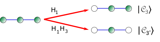
Figure 5: Schematic diagram representing the transformation of 3-hybrid-qubit cluster state into $\left|\mathcal{C}_{3}\right\rangle$ and $\left|\mathcal{C}_{3^{\prime}}\right\rangle$. ${\rm H}_{1}$ and ${\rm H}_{3}$ are the Hadamard operations on the first and the third (from the left) modes of the hybrid qubit, respectively. A unfilled circle represents the action of a Hadamard transform.

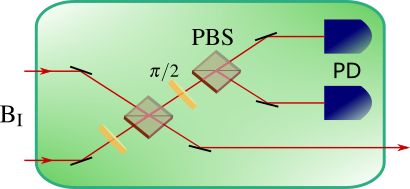
Figure 6: $\mathrm{B}_{\mathrm{I}}$ is an entangling operation, which acts on the DV modes of hybrid qubits and outputs one mode. Two PDs follow two polarizing beam splitter (PBS) with two $\pi/2$-rotators (wave plates) as shown in the figure. $\mathrm{B}_{\mathrm{I}}$ is successful with probability $1/2$ only when one of the PDs clicks.

The state $\left|\mathcal{C}_{3}\right\rangle$ is generated by entangling three $|+_{\rm L}^{\sqrt{2}\alpha}\rangle$’s (hybrid qubit with CV mode of amplitude $\sqrt{2}\alpha$) and a $|+_{\rm L}\rangle$ using two $\mathrm{B}_{\alpha}\,$’s and a $\mathrm{B}_{\mathrm{I}}$. As shown in Fig. 6, $\mathrm{B}_{\mathrm{I}}$ has two polarizing BSs (PBS), $\frac{\pi}{2}$-rotators and and two photon detectors (PD). PBS transmits $\left|\textsc{v}\right\rangle$ and reflects $\left|\textsc{h}\right\rangle$. $\mathrm{B}_{\mathrm{I}}$ performs the operation $\left|\textsc{h}\right\rangle\langle\textsc{h},\textsc{h}|+\left|\textsc{h}\right\rangle\langle\textsc{h},\textsc{v}|+\left|\textsc{v}\right\rangle\langle\textsc{v},\textsc{h}|-\left|\textsc{v}\right\rangle\langle\textsc{v},\textsc{v}|$ which succeeds with probability 1/2 only when one of the PDs click. Instances with no click and both PDs clicking are failures. Hybrid qubits are initialized as $|+_{\rm L}^{\sqrt{2}\alpha}\rangle\otimes|+_{\rm L}^{\sqrt{2}\alpha}\rangle\otimes|+_{\rm L}\rangle\otimes|+_{\rm L}^{\sqrt{2}\alpha}\rangle$ and passed on to beam splitters as shown in Fig. 7. The resulting state of the hybrid qubits is

$$\left|\alpha,\alpha,\alpha,\alpha,\alpha,\alpha,\alpha\right\rangle\left|\textsc{h},\textsc{h},\textsc{h},\textsc{h}\right\rangle$$

$$+\left|\alpha,\alpha,\alpha,\alpha,\alpha,-\alpha,-\alpha\right\rangle\left|\textsc{h},\textsc{h},\textsc{h},\textsc{v}\right\rangle$$

$$+\left|\alpha,\alpha,\alpha,\alpha,-\alpha,\alpha,\alpha\right\rangle\left|\textsc{h},\textsc{h},\textsc{v},\textsc{h}\right\rangle$$

$$+\left|\alpha,\alpha,\alpha,\alpha,-\alpha,-\alpha,-\alpha\right\rangle\left|\textsc{h},\textsc{h},\textsc{v},\textsc{v}\right\rangle$$

$$+\left|\alpha,\alpha,-\alpha,-\alpha,\alpha,\alpha,\alpha\right\rangle\left|\textsc{h},\textsc{v},\textsc{h},\textsc{h}\right\rangle$$

$$+\left|\alpha,\alpha,-\alpha,-\alpha,\alpha,-\alpha,-\alpha\right\rangle\left|\textsc{h},\textsc{v},\textsc{h},\textsc{v}\right\rangle$$

$$+\left|\alpha,\alpha,-\alpha,-\alpha,-\alpha,\alpha,\alpha\right\rangle\left|\textsc{h},\textsc{v},\textsc{v},\textsc{h}\right\rangle$$

$$+\left|\alpha,\alpha,-\alpha,-\alpha,-\alpha,-\alpha,-\alpha\right\rangle\left|\textsc{h},\textsc{v},\textsc{v},\textsc{v}\right\rangle$$

$$+\left|-\alpha,-\alpha,\alpha,\alpha,\alpha,\alpha,\alpha\right\rangle\left|\textsc{v},\textsc{h},\textsc{h},\textsc{h}\right\rangle$$

$$+\left|-\alpha,-\alpha,\alpha,\alpha,\alpha,-\alpha,-\alpha\right\rangle\left|\textsc{v},\textsc{h},\textsc{h},\textsc{v}\right\rangle$$

$$+\left|-\alpha,-\alpha,\alpha,\alpha,-\alpha,\alpha,\alpha\right\rangle\left|\textsc{v},\textsc{h},\textsc{v},\textsc{h}\right\rangle$$

$$+\left|-\alpha,-\alpha,\alpha,\alpha,-\alpha,-\alpha,-\alpha\right\rangle\left|\textsc{v},\textsc{h},\textsc{v},\textsc{v}\right\rangle$$

$$+\left|-\alpha,-\alpha,-\alpha,-\alpha,\alpha,\alpha,\alpha\right\rangle\left|\textsc{v},\textsc{v},\textsc{h},\textsc{h}\right\rangle$$

$$+\left|-\alpha,-\alpha,-\alpha,-\alpha,\alpha,-\alpha,-\alpha\right\rangle\left|\textsc{v},\textsc{v},\textsc{h},\textsc{v}\right\rangle$$

$$+\left|-\alpha,-\alpha,-\alpha,-\alpha,-\alpha,\alpha,\alpha\right\rangle\left|\textsc{v},\textsc{v},\textsc{v},\textsc{h}\right\rangle$$

$$+\left|-\alpha,-\alpha,-\alpha,-\alpha,-\alpha,-\alpha,-\alpha\right\rangle\left|\textsc{v},\textsc{v},\textsc{v},\textsc{v}\right\rangle.$$ (4)

Upon successful $\mathrm{B}_{\alpha}\,(2,3)$ and $\mathrm{B}_{\alpha}\,(5,6)$ with respective outcomes, say $\left|\psi^{+}\right\rangle$ and $\left|\psi^{+}\right\rangle$, the state in Eq. (B) reduces to

$$\left|\alpha,\alpha,\alpha\right\rangle\left|\textsc{h},\textsc{h},\textsc{h},\textsc{h}\right\rangle+\left|\alpha,\alpha,-\alpha\right\rangle\left|\textsc{h},\textsc{h},\textsc{v},\textsc{v}\right\rangle+$$

$$\left|-\alpha,-\alpha,\alpha\right\rangle\left|\textsc{v},\textsc{v},\textsc{h},\textsc{h}\right\rangle+\left|-\alpha,-\alpha,-\alpha\right\rangle\left|\textsc{v},\textsc{v},\textsc{v},\textsc{v}\right\rangle,$$

where $\mathrm{B}_{\alpha}\,(n,m)$ represents the action of $\mathrm{B}_{\alpha}\,$ on $n$-th and $m$-th CV modes as shown in the Fig. 7. Further, with the successful $\mathrm{B}_{\mathrm{I}}(2,3)$ (DV modes 2 and 3 being the inputs as shown in the Fig. 7) we get

$$\left|\mathcal{C}_{3}\right\rangle=\left|\alpha,\alpha,\alpha\right\rangle\left|\textsc{h},\textsc{h},\textsc{h}\right\rangle+\left|\alpha,\alpha,-\alpha\right\rangle\left|\textsc{h},\textsc{h},\textsc{v}\right\rangle+$$

$$\left|-\alpha,-\alpha,\alpha\right\rangle\left|\textsc{v},\textsc{v},\textsc{h}\right\rangle-\left|-\alpha,-\alpha,-\alpha\right\rangle\left|\textsc{v},\textsc{v},\textsc{v}\right\rangle.$$ (5)

Note that for other possible measurement outcomes on $\mathrm{B}_{\alpha}\,$ and $\mathrm{B}_{\mathrm{I}}$, the $\left|\mathcal{C}_{3}\right\rangle$ will be equivalent up to local Pauli operations. The local operations to be performed upon getting different measurement comes are listed in Table 1. The logical Pauli operations on hybrid qubits can be accomplished with the polarization rotator on the DV mode and the $\pi$-phase shifter on the CV mode. $X_{\textrm{L}}$: $\left|\alpha\right\rangle\leftrightarrow\left|-\alpha\right\rangle,~{}\left|\textsc{h}\right\rangle\leftrightarrow\left|\textsc{v}\right\rangle$ and $Z_{\textrm{L}}$: $\left|\textsc{h}\right\rangle\rightarrow\left|\textsc{h}\right\rangle$, $\left|\textsc{v}\right\rangle\rightarrow-\left|\textsc{v}\right\rangle$ with no need for action on $\left|\alpha\right\rangle$. These local operations are used only in creating the offline resource states, which is not a ballistic process.

Similarly, state $\left|\mathcal{C}_{3^{\prime}}\right\rangle$ can be generated by removing the $\pi/2$-rotator at the input of the $\mathrm{B}_{\mathrm{I}}$ in Fig. 6. Here, the only other possible outcome on the $\mathrm{B}_{\alpha}\,$s is $\left|\psi^{-}\right\rangle$, in which case the relative phase can be changed by applying a $Z_{\rm L}$ for the measurement outcome combination $\{\left|\psi^{\pm}\right\rangle,\left|\psi^{\mp}\right\rangle\}$. The kets $\left|\mathcal{C}_{3}\right\rangle$ and $\left|\mathcal{C}_{3^{\prime}}\right\rangle$ are created only when the operations $\mathrm{B}_{\alpha}\,$ and $\mathrm{B}_{\mathrm{I}}$ succeed together. The probability that all the three operations are successful is $\frac{1}{2}(1-e^{-2\alpha^{2}})^{2}$. Thus, the average number of hybrid qubits consumed for generating a $\left|\mathcal{C}_{3}\right\rangle$ or $\left|\mathcal{C}_{3^{\prime}}\right\rangle$ is $8/(1-e^{-2\alpha^{2}})^{2}$.

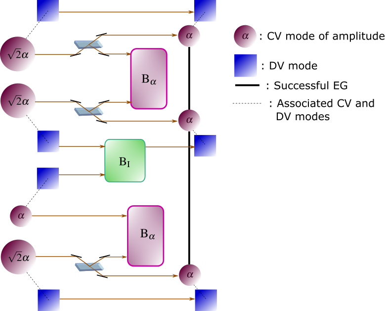
Figure 7: A schematic diagram to build the offline resource state $\left|\mathcal{C}_{3}\right\rangle$ using two $\mathrm{B}_{\alpha}\,$’s, one $\mathrm{B}_{\mathrm{I}}$, three 1:1 beam splitters and four hybrid qubits, and EO represents entangling operation. To create $\left|\mathcal{C}_{3^{\prime}}\right\rangle$, the ${\pi}/{2}$-rotator at the input of the $\mathrm{B}_{\mathrm{I}}$ is removed.

$\rm B_{\alpha}(2,3)$	$\rm B_{\alpha}(5,6)$	$\mathrm{B}_{\mathrm{I}}(2,3)$	Local Operation
$\left|\psi^{+}\right\rangle$	$\left|\psi^{+}\right\rangle$	h/v	NA/$Z_{3}$
$\left|\psi^{+}\right\rangle$	$\left|\psi^{-}\right\rangle$		$Z_{3}$/$Z_{2}Z_{3}$
$\left|\psi^{+}\right\rangle$	$\left|\phi^{+}\right\rangle$		$Z_{2}$/NA
$\left|\psi^{+}\right\rangle$	$\left|\phi^{-}\right\rangle$		$Z_{2}Z_{3}$/$X_{3}Z_{2}Z_{3}$
$\left|\psi^{-}\right\rangle$	$\left|\psi^{+}\right\rangle$	h/v	$Z_{2}$/NA
$\left|\psi^{-}\right\rangle$	$\left|\psi^{-}\right\rangle$		$Z_{2}Z_{3}$/$Z_{3}$
$\left|\psi^{-}\right\rangle$	$\left|\phi^{+}\right\rangle$		NA/$Z_{2}$
$\left|\psi^{-}\right\rangle$	$\left|\phi^{-}\right\rangle$		$X_{3}Z_{2}Z_{3}$/$Z_{2}Z_{3}$
$\left|\phi^{+}\right\rangle$	$\left|\psi^{+}\right\rangle$	h/v	$X_{1}$/$X_{1}Z_{1}$
$\left|\phi^{+}\right\rangle$	$\left|\psi^{-}\right\rangle$		$X_{2}$/$X_{1}Z_{2}Z_{3}$
$\left|\phi^{+}\right\rangle$	$\left|\phi^{+}\right\rangle$		$X_{1}Z_{2}$/$X_{1}$
$\left|\phi^{+}\right\rangle$	$\left|\phi^{-}\right\rangle$		$X_{1}Z_{2}Z_{3}$/$X_{1}Z_{3}$
$\left|\phi^{-}\right\rangle$	$\left|\psi^{+}\right\rangle$	h/v	$X_{2}Z_{2}Z_{3}$/$X_{1}$
$\left|\phi^{-}\right\rangle$	$\left|\psi^{-}\right\rangle$		$X_{2}Z_{2}$/$X_{2}$
$\left|\phi^{-}\right\rangle$	$\left|\phi^{+}\right\rangle$		$X_{1}$/$X_{1}Z_{2}$
$\left|\phi^{-}\right\rangle$	$\left|\phi^{-}\right\rangle$		$X_{2}$/$X_{1}Z_{2}Z_{3}$

Table 1: The table lists the local operations to be performed upon getting different measurement comes on $\mathrm{B}_{\alpha}\,$ and $\mathrm{B}_{\mathrm{I}}$

Appendix C Hybrid qubits under photon loss

The action of the photon-loss channel $\mathcal{E}$ on a hybrid qubit initialized in the state $\rho_{0}=\left|+_{\rm L}\right\rangle\langle+_{\rm L}|$ is Lee and Jeong (2013)

$$\mathcal{E}(\rho_{0}) =(1-\eta)\bigg{(}\frac{1+e^{-2\eta\alpha^{2}}}{2}\left|+^{\prime}\right\rangle\langle+^{\prime}|+$$ (6)

$$+\frac{1-e^{-2\eta\alpha^{2}}}{2}\left|-^{\prime}\right\rangle\langle-^{\prime}|\bigg{)}+\frac{\eta}{2}\left(|+^{\rm lk}\rangle\langle+^{\rm lk}|+|-^{\rm lk}\rangle\langle-^{\rm lk}|\right)$$

$$= \frac{(1-\eta)}{2}\bigg{(}|\alpha^{\prime},\textsc{h}\rangle\langle\alpha^{\prime},\textsc{h}|+|-\alpha^{\prime},\textsc{v}\rangle\langle-\alpha^{\prime},\textsc{v}|$$

$$+ e^{-2\eta\alpha^{2}}\big{(}|\alpha^{\prime},\textsc{h}\rangle\langle-\alpha^{\prime},\textsc{v}|+|-\alpha^{\prime},\textsc{v}\rangle\langle\alpha^{\prime},\textsc{h}|\big{)}\bigg{)}$$

$$+ \frac{\eta}{2}\bigg{(}\big{(}|\alpha^{\prime}\rangle\langle\alpha^{\prime}|+|-\alpha^{\prime}\rangle\langle-\alpha^{\prime}|\big{)}\otimes\left|0\right\rangle\langle 0|\bigg{)}$$

where $\left|\pm^{\prime}\right\rangle=(\left|\alpha^{\prime},\textsc{h}\right\rangle\pm\left|-\alpha^{\prime},\textsc{v}\right\rangle)/\sqrt{2},~{}\left|\pm^{\rm lk}\right\rangle=(\left|\alpha^{\prime}\right\rangle\pm\left|-\alpha^{\prime}\right\rangle)\otimes\left|0\right\rangle/\sqrt{2}$ and $\alpha^{\prime}=\sqrt{1-\eta}\alpha$ with $\eta$ being photon loss rate which also models imperfect sources, detectors, or absorptive optical components. It can be seen from the Eq. (6), that due to photon loss the CV part is dephased, i.e., a phase flip error $Z$ occurs on the hybrid qubits and the loss on the DV part makes them leak out of the logical basis. Also, due to photon losses the success rate of the $\mathrm{B}_{\alpha}\,$ reduces to $(1-e^{-2\alpha^{\prime 2}})$ and that of $\mathrm{B}_{\mathrm{I}}$ remains same. As a result, the average number of hybrid qubits to build off-line resource states increases to $8/[(1-e^{-2\alpha^{\prime 2}})^{2}]$. The failure rate of the HBSM, $p_{f}$ increases to $(1-\eta)\mathrm{e}^{\mbox{\footnotesize$-2\alpha^{\prime 2}$}}/2+\eta\mathrm{e}^{\mbox{\footnotesize$-2\alpha^{\prime 2}$}}=(1+\eta)\mathrm{e}^{\mbox{\footnotesize$-2\alpha^{\prime 2}$}}/2$, where $\alpha^{\prime}=\sqrt{1-\eta}\alpha$. The first term originates from the attenuation of CV mode, and the second from both CV attenuation and DV loss.

Loss-tolerance of $\mathrm{B}_{\mathrm{I}}$: One can verify that the noisy DV part in Eq. (B), $\mathcal{E}^{\otimes 4}(\left|\textsc{h},\textsc{h},\textsc{h},\textsc{h}\right\rangle+\left|\textsc{h},\textsc{h},\textsc{v},\textsc{v}\right\rangle+\left|\textsc{v},\textsc{v},\textsc{h},\textsc{h}\right\rangle+\left|\textsc{v},\textsc{v},\textsc{v},\textsc{v}\right\rangle)$ is transformed in to $\mathcal{E}^{\otimes 3}(\left|\textsc{h},\textsc{h},\textsc{h}\right\rangle+\left|\textsc{h},\textsc{h},\textsc{v}\right\rangle+\left|\textsc{v},\textsc{v},\textsc{h}\right\rangle-\left|\textsc{v},\textsc{v},\textsc{v}\right\rangle)$ under the action of $\mathrm{B}_{\mathrm{I}}$. The noise channel on the resulting state is still $\mathcal{E}$, implying that no additional computational errors are introduced by $\mathrm{B}_{\mathrm{I}}$, unlike in Ref. Li et al. (2015).

C.1 Noise by HBSM under photo-loss

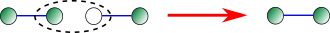
Figure 8: Typical instance of action of HBSM on the noisy hybrid cluster states.

Let us consider the typical situation where HBSMs are used to create entanglement between the desired hybrid qubits as shown in the Fig. 8. Looking at only the CV part, we have

$$(\left|\alpha,\alpha\right\rangle+\left|\alpha,-\alpha\right\rangle+\left|-\alpha,\alpha\right\rangle-\left|-\alpha,-\alpha\right\rangle)(\left|\alpha,\alpha\right\rangle+(\left|-\alpha,-\alpha\right\rangle).$$ (7)

To determine the noise on the resultant cluster state after the action of $\mathrm{B}_{\alpha}\,$, we consider the hybrid qubits undergoing BSM to be noisy. The resulting noisy state, in the logical basis is of the form

$$\frac{1}{4}\begin{pmatrix}1&e^{-4\eta\alpha^{2}}&1&e^{-4\eta\alpha^{2}}\\ e^{-4\eta\alpha^{2}}&1&e^{-4\eta\alpha^{2}}&1\\ 1&e^{-4\eta\alpha^{2}}&1&e^{-4\eta\alpha^{2}}\\ e^{-4\eta\alpha^{2}}&1&e^{-4\eta\alpha^{2}}&1\end{pmatrix}.$$ (8)

For the desired result of the HBSMs, the Hadamard could be on the other hybrid qubit too where the terms in the Eq. 7 are interchanged and the resulting noisy sate is

$$\frac{1}{4}\begin{pmatrix}1&1&e^{-4\eta\alpha^{2}}&e^{-4\eta\alpha^{2}}\\ 1&1&e^{-4\eta\alpha^{2}}&e^{-4\eta\alpha^{2}}\\ e^{-4\eta\alpha^{2}}&e^{-4\eta\alpha^{2}}&1&1\\ e^{-4\eta\alpha^{2}}&e^{-4\eta\alpha^{2}}&1&1\\ \end{pmatrix}.$$ (9)

Considering both the instances of action of $\mathrm{B}_{\alpha}\,$, the resultant state is the equal weighted superposition of the states in Eqs. (8) and (9), and the corresponding Kraus operators for this noisy channel $\mathcal{E}^{\mathrm{B}_{\alpha}\,}$ are $\Big{\{}\sqrt{\frac{1+e^{-4\eta\alpha^{2}}}{2}}I\otimes I,~{}~{}\sqrt{\frac{1-e^{-4\eta\alpha^{2}}}{4}}Z\otimes I,~{}~{}\sqrt{\frac{1-e^{-4\eta\alpha^{2}}}{4}}I\otimes Z\Big{\}}$. This noise channel $\mathcal{E}^{\mathrm{B}_{\alpha}\,}$ is used as the noise due to entangling operation in the AUTOTUNE Fowler et al. (2012). We observe that for $\eta\sim 10^{-3}$ and small values of $\alpha$, $p_{Z}\approx(1-e^{-4\eta\alpha^{2}})/4$. Thus, the $\mathcal{E}^{\mathrm{B}_{\alpha}\,}$ will have the following Kraus operators $\{\sqrt{(1-2p_{Z})}~{}I\otimes I,~{}~{}\sqrt{p_{Z}}~{}Z\otimes I,~{}~{}\sqrt{p_{Z}}~{}I\otimes Z\}$.

Loss-tolerance of $\rm B_{s}$: Now, let us move our attention towards the DV part of the noisy cluster states as shown in the Fig. 8 and study the action of ${\rm B_{s}}$ on them during photon loss. One can verify that the state $\mathcal{E}\big{(}\left|\textsc{h},\textsc{h}\right\rangle+\left|\textsc{v},\textsc{v}\right\rangle\big{)}\otimes\big{(}\left|\textsc{h},\textsc{h}\right\rangle+\left|\textsc{h},\textsc{v}\right\rangle+\left|\textsc{v},\textsc{h}\right\rangle-\left|\textsc{v},\textsc{v}\right\rangle\big{)}$ is transformed to $\mathcal{E}\big{(}|\textsc{h},\textsc{h}\rangle+|\textsc{h},\textsc{v}\rangle+|\textsc{v},\textsc{h}\rangle-|\textsc{v},\textsc{v}\rangle\big{)}$ under the action of ${\rm B_{s}}$. The noise channel on the resulting state is still $\mathcal{E}$ which confirms that the ${\rm B_{s}}$ introduces no additional computational errors.

Appendix D Short note on simulation with AUTOTUNE

To simulate topological quantum error correction (QEC) on a noisy $|\mathcal{C}_{\mathcal{L}}\rangle$, we use the software package AUTOTUNE Fowler et al. (2012) which offers a wide range of options of noise models and the ability to customize them. Remarkably, it allows for simulation of QEC when some qubits on $|\mathcal{C}_{\mathcal{L}}\rangle$ are missing. This feature allows us to simulate missing edges by mapping them to missing qubits as explained in the main Letter. AUTOTUNE uses the circuit model to simulate the error propagation while building $|\mathcal{C}_{\mathcal{L}}\rangle$.

A noisy $|\mathcal{C}_{\mathcal{L}}\rangle$ can be simulated using AUTOTUNE in the following way. We notice that in order to generate $|\mathcal{C}_{\mathcal{L}}\rangle$, the action of HBSMs for creating edges between the central hybrid qubits of $|\mathcal{C}_{\ast}\rangle$ (see Fig. 1(b) of the main Letter) is the equivalent to the action of controlled-Z (CZ) gates on qubits all initialized in $\left|+\right\rangle$’s (eigenstates of Pauli-X operator with eigenvalue +1) on the lattice in the circuit model. So, the action of HBSMs under noise can be simulated by noisy CZ gates in AUTOTUNE and thereafter the whole QEC. Also, AUTOTUNE allows for the simulation of the noise added during the initialization of the qubits, noisy gate operations, and error propagation through the lattice.

AUTOTUNE used for simulation is optimized compared to the one used in Ref. Herrera-Martí et al. (2010). In the decoding process, AUTOTUNE uses additional diagonal links compared to Manhattan lattice Fowler et al. (2012). These diagonal links avoid the wrong identification of error chains by the minimum-weight perfect-match algorithm and guarantee corrections of $(d-1)/2$ errors to improve the accuracy in estimating the logical error rate $p_{\rm L}$. These details are in Sec. IV of Ref. Fowler et al. (2012). Thus the results obtained from the simulations of the topological QEC corresponding to code distances $d=5,7,9$ are reliable and the finite-size effect is negligible. An example for this is Ref. Whiteside and Fowler (2014) which uses AUTOTUNE to extrapolates the behaviors of higher distances from that of $d=5,7$ and sometimes $d=9$.

In HTQC, mapping the missing edges (due to failed HBSMs) to missing qubits is a crucial part in the simulation of QEC on a noisy $|\mathcal{C}_{\mathcal{L}}\rangle$. The HBSMs are used in two cases: (a) building star cluster $\left|\mathcal{C}_{\ast}\right\rangle$ and (b) connecting the $\left|\mathcal{C}_{\ast}\right\rangle$’s as shown in Fig. 2(b) of the main Letter. In the first case, failure of an HBSM creates a diagonal edge that must be removed by measuring the two qubits in the Z-basis, $M_{z}$, as shown in Fig. 2(c) of the main Letter. Thus, in the first case of failure of an HBSM, a missing edge corresponds to two missing qubits. In the second case, failure of an HBSM leads to a missing edge between the qubits as shown in Fig. 2(a) of the main Letter. During QEC one of the qubits associated with the missing edge is removed by $M_{z}$. Thus, in the second case of failure, a missing edge corresponds to one missing qubit.

In a lattice $|\mathcal{C}_{\mathcal{L}}\rangle$ of distance $d$, one can count that there are $6d^{3}$ qubits connected by $12d^{3}$ edges as done in Sec. VIII of Ref. Whiteside and Fowler (2014). In this approach, a lattice of distance $d$, there are $d^{3}$ unit cells, and each unit cell has effectively 6 qubits Whiteside and Fowler (2014). Each face of the unit cell has four edges shared between two faces. Thus each face has effectively two edges. Thus a unit cell has on average 12 edges.

A star cluster state $\left|\mathcal{C}_{\ast}\right\rangle$ corresponds to one lattice qubit, and two HBSMs are used for building the star cluster state. Thus, an equal number (i.e., $12d^{3}$ per lattice state $|\mathcal{C}_{\mathcal{L}}\rangle$) of HBSMs are used for creation of $|\mathcal{C}_{\ast}\rangle$’s and for connecting them in HTQC. Considering both the cases of usage of HBSMs, on average 1.5 qubits are lost per HBSM failure.

As pointed out in the result section of the main Letter, the target error rate is estimated using the suppression ratio of $p_{\rm L}$ with $d$. As AUTOTUNE uses the minimum-weight perfect-match algorithm, the suppression ratio is expected to be nearly constant when it is sufficiently away from the threshold and $d$ is large Whiteside and Fowler (2014); Fowler (2012). If the suppression ratio is not constant, resource estimation will lead to an underestimation. From the simulation results, we have the suppression ratio between distances 3 and 5 to be $a/a^{\prime}\approx 12.5$, between 5 and 7 to be $a/a^{\prime}\approx 6.1$, and between 7 and 9 to be $a/a^{\prime}\approx 5.6$. We observe that the suppression ratio is nearly constant between distances 5 and 7 (7 and 9). Thus we choose the suppression ratio between the distances 7 and 9, i.e., $a/a^{\prime}\approx 5.6$ to estimate target $p_{\rm L}$ and resource overheads.

We observe from Fig. 3(a) of the main Letter that if we add curves of higher values of $d$, the threshold point $p_{Z,\rm th}$ would tend to shift towards the higher side. The same can be observed from Fig. 10 of Ref. Raussendorf et al. (2007). However, taking a conservative approach we consider the value of $p_{Z,{\rm th}}$ to be $6.9\times 10^{-3}$, which corresponds to photon-loss threshold of $\eta_{\rm th}=3.3\times 10^{-3}$.

Appendix E Resource efficiency of HTQC against unreported schemes

There are no reports estimating resource $N$ to attain a logical error rate $p_{\rm L}$ of $10^{-6}$ or $10^{-15}$ for PLOQC, MQQC, HQQC and TPQC. The first three schemes are based on the 7-qubit Steane code which has a typical value of $p_{\rm L}\sim 10^{-3}$ for the first level of telecorrection and needs more levels of concatenation to reach a smaller value of $p_{\rm L}$. Typically, 4 levels suffice to attain $p_{\rm L}\sim 10^{-6}$ Dawson et al. (2006); Lund et al. (2008). In what follows, we make an informed guess to justify the resource efficiency of HTQC.

1. The first level of telecorrection in HQQC needs approximately $5.35\times 10^{3}$ hybrid-qubits (with $\alpha=1.1$) Lee and Jeong (2013). The number of hybrid-qubits incurred per operation, at a particular level L, is given by the number of hybrid-qubits consumed per error correction step at first level, multiplied by number of operations needed at levels $2,\dots,L$ Dawson et al. (2006). Typically, error correction at first level requires 1000 operations [10]. Here, we assume that level 2,3 would require 100 operations and make resource estimation similar to that in Ref. Lee and Jeong (2013) for first level. Roughly speaking, adding another 3 levels would cost $N\approx 8\times 10^{9}$ which shows that the HTQC is more resource-efficient.

2. MOQC requires the following multi-mode optical resource states (upto normalization) for optimal loss-threshold Lee et al. (2015):

   $$\left|Z\right\rangle\equiv\left|+\right\rangle^{\otimes 4}\left|+\right\rangle^{\otimes 4}+\left|+\right\rangle^{\otimes 4}\left|-\right\rangle^{\otimes 4}+\left|-\right\rangle^{\otimes 4}\left|+\right\rangle^{\otimes 4}-\left|-\right\rangle^{\otimes 4}\left|-\right\rangle^{\otimes 4}$$

   $$\left|Z^{\prime}\right\rangle\equiv\left|+\right\rangle^{\otimes 8}\left|+\right\rangle^{\otimes 8}+\left|+\right\rangle^{\otimes 8}\left|-\right\rangle^{\otimes 8}+\left|-\right\rangle^{\otimes 8}\left|+\right\rangle^{\otimes 8}-\left|-\right\rangle^{\otimes 8}\left|-\right\rangle^{\otimes 8},$$

   where $\left|\pm\right\rangle=(\left|\textsc{h}\right\rangle\pm\left|\textsc{v}\right\rangle)/\sqrt{2}$. Using ${\rm B_{I}}$ of success rate 0.5 and ${\rm B_{s}}$ of boosted success rate 0.75 on the supply of Bell states, $\left|Z\right\rangle$ and $\left|Z^{\prime}\right\rangle$ can be constructed. Let’s denote the $n$-mode GHZ state by $\left|{\rm GHZ}_{n}\right\rangle=\left|\textsc{h}\right\rangle^{\otimes n}+\left|\textsc{v}\right\rangle^{\otimes n}$ (upto normalization).

   To generate $\left|Z\right\rangle$, we fuse $\left|{\rm GHZ}_{6}\right\rangle$ and $\left|{\rm GHZ}_{4}\right\rangle$ using ${\rm B_{s}}$ with a Hadamard operation on the first mode of the latter state. The resulting state would be equivqlent to the $\left|Z\right\rangle$ upto local Hadamard operations. In prior, the $\left|{\rm GHZ}_{4}\right\rangle$ is generated with two $\left|{\rm GHZ}_{3}\right\rangle$ using a ${\rm B_{s}}$’s. Thus, on average $2/0.75$ number of $\left|{\rm GHZ}_{3}\right\rangle$ are needed. On the other hand, $\left|{\rm GHZ}_{6}\right\rangle$ is created by fusing two $\left|{\rm GHZ}_{4}\right\rangle$’s using a ${\rm B_{s}}$’s, which requires, on average, $(2/0.75)^{2}$ number of $\left|{\rm GHZ}_{3}\right\rangle$’s. Finally, $\left|Z\right\rangle$ needs, on average, $\frac{1}{0.75}\big{(}\frac{2}{0.75^{2}}+\frac{2}{0.75}\big{)}$ number of $\left|{\rm GHZ}_{3}\right\rangle$’s. Each $\left|{\rm GHZ}_{3}\right\rangle$ can be generated using ${\rm B_{I}}$ and needs four Bell states, on average. Additionally, 8 Bell states are spent for boosting the success rate of $\rm B_{s}$ Grice (2011). Totally, $\frac{1}{0.75}\big{(}(\frac{2}{0.75})^{2}+\frac{2}{0.75}\big{)}\times 4+8\approx 60$ Bell states are consumed to generate $\left|Z\right\rangle$.

   To generate $\left|Z^{\prime}\right\rangle$, one needs to fuse $\left|{\rm GHZ}_{10}\right\rangle$ and $\left|{\rm GHZ}_{8}\right\rangle$ using ${\rm B_{s}}$ with a Hadamard operation on the first mode of the latter state. On average, $(2/0.75)^{3}$ number of $\left|{\rm GHZ}_{3}\right\rangle$’s are needed to generate a $\left|{\rm GHZ}_{10}\right\rangle$. Following the calculation carried out in the case of generating $\left|Z\right\rangle$, finally, $\frac{1}{0.75}\big{[}(\frac{2}{0.75})^{3}+\frac{1}{0.75}\big{(}(\frac{2}{0.75})^{2}+\frac{2}{0.75}\big{)}\big{]}\times 4+16\approx 187$ number of Bell states are incurred to build $\left|Z^{\prime}\right\rangle$.

   Following the procedure to calculate the resource cost as per Ref. Lee and Jeong (2013), first level of error correction needs $7.2\times 10^{4}$ Bell states. Arguing similar to the case of HQQC, adding another 3 levels would cost $N\approx 2.7\times 10^{14}$. Thus, HTQC is better than MQQC in terms of resource efficiency.

3. For PLOQC, $N\approx 1.8\times 10^{5}$ just for the first level of telecorrection Hayes et al. (2010), and making argument similar to HQQC, resource incurred for 4 levels would be larger by many orders of magnitude. Hence, HTQC is more resource-efficient.

4. By extrapolating the suppression of $p_{\rm L}$ with $d$, we estimate $d$ required to achieve the target $p_{\rm L}\approx 10^{-6}(10^{-15})$ using the expression Whiteside and Fowler (2014),

   $$p_{\rm L}=\frac{a^{\prime}}{(\frac{a}{a^{\prime}})^{(d-d_{a^{\prime}})/2}},$$ (10)

   where $a$ and $a^{\prime}$ are the values of $p_{\rm L}$ corresponding to the second highest distance, $d_{a}$, and the highest distance, $d_{a^{\prime}}$, chosen for the simulation. For the topological photonic QC (TPQC), we can make resource estimation by looking at Figs. 7(a) and (b) of Ref. Herrera-Martí et al. (2010).

   First, we look into Fig. 7(a) of Ref. Herrera-Martí et al. (2010) that plots $p_{\rm L}$ against computational error rate and corresponds to the case with no photon loss (qubit loss). Here, $a\approx 0.065$ (corresponding to $d_{a}=13$) and $a^{\prime}\approx 0.059$ (corresponding to $d_{a^{\prime}}=15$). Using Eq. (10) above, we find that a $\left|\mathcal{C}_{\mathcal{L}}\right\rangle$ of $d\approx 225~{}(621)$ is essential to attain $p_{\rm L}\sim 10^{-6}~{}(10^{-15})$. In TPQC, redundantly encoded photons are used as a qubit in the $\left|\mathcal{C}_{\mathcal{L}}\right\rangle$ and to maximize the probability of the edge creation between the qubits. To create an edge successfully, the entangling operation is performed $R$ times. On average, this requires a qubit to consist of $2R+1$ photons Herrera-Martí et al. (2010). We know that a $\left|\mathcal{C}_{\mathcal{L}}\right\rangle$ of side $5d/4$ would have $6\times(5d/4)^{3}$ qubits, on average. In TPQC the redundant encoded photons are considered as resources. Thus, the incurred resource overhead in TPQC would be $N=(2R+1)\times 6\big{(}\frac{5d}{4}\big{)}^{3}$. For optimal $\eta_{\rm th}$, $R$ is set to 7 in TPQC Herrera-Martí et al. (2010), and we obtain $N\approx 2\times 10^{9}~{}(4.2\times 10^{10})$ for $d=225~{}(621)$.

   Next, we consider Fig. 7(b) of Ref. Herrera-Martí et al. (2010) where $p_{\rm L}$ is plotted against photon loss (qubit loss). We emphasize that in this plot there is no computational error introduced. Here, we have $a\approx 0.015$ (corresponding to $d_{a}=13$) and $a^{\prime}\approx 0.01$ (corresponding to $d_{a^{\prime}}=15$). Using Eq. (10), it is found that $\left|\mathcal{C}_{\mathcal{L}}\right\rangle$ of $d\approx 60~{}(162)$ is essential to attain $p_{\rm L}\sim 10^{-6}~{}(10^{-15})$. In this case of TPQC we get $N\approx 3.8\times 10^{7}~{}(7.5\times 10^{8})$.

   Both the computational errors and the photon losses are considered together for estimating resource overheads of all the other schemes. If both the factors are considered for TPQC, the incurred resources would be much more than $2\times 10^{9}~{}(4.2\times 10^{10})$ to attain $p_{\rm L}\sim 10^{-6}~{}(10^{-15})$. This means that HTQC offers a resource efficiency better than that of TPQC at least by 3 orders of magnitude. We note that considering only the factor of photon loss would lead to an underestimation of the resource overhead for TPQC.

References

- Nielsen and Chuang (2010) M. A. Nielsen and I. L. Chuang, Quantum Computation and Quantum Information (Cambridge University Press, 2010).
- Lidar and Brun (eds.) D. A. Lidar and T. A. Brun (eds.), Quantum Error Correction (Cambridge University Press, 2013).
- Raussendorf et al. (2006) R. Raussendorf, J. Harrington, and K. Goyal, Annals of Physics 321, 2242 (2006).
- Raussendorf et al. (2007) R. Raussendorf, J. Harrington, and K. Goyal, New Journal of Physics 9, 199 (2007).
- Raussendorf and Harrington (2007) R. Raussendorf and J. Harrington, Phys. Rev. Lett. 98, 190504 (2007).
- Barrett and Stace (2010) S. D. Barrett and T. M. Stace, Phys. Rev. Lett. 105, 200502 (2010).
- Whiteside and Fowler (2014) A. C. Whiteside and A. G. Fowler, Phys. Rev. A 90, 052316 (2014).
- Li et al. (2010) Y. Li, S. D. Barrett, T. M. Stace, and S. C. Benjamin, Phys. Rev. Lett. 105, 250502 (2010).
- Briegel and Raussendorf (2001) H. J. Briegel and R. Raussendorf, Phys. Rev. Lett. 86, 910 (2001).
- Ralph and Pryde (2010) T. C. Ralph and G. J. Pryde, Progress in Optics, 54, 209 (2010).
- Browne and Rudolph (2005) D. E. Browne and T. Rudolph, Phys. Rev. Lett. 95, 010501 (2005).
- Nielsen (2004) M. A. Nielsen, Phys. Rev. Lett. 93, 040503 (2004).
- Dawson et al. (2006) C. M. Dawson, H. L. Haselgrove, and M. A. Nielsen, Phys. Rev. A 73, 052306 (2006).
- Fujii and Tokunaga (2010) K. Fujii and Y. Tokunaga, Phys. Rev. Lett. 105, 250503 (2010).
- Herrera-Martí et al. (2010) D. A. Herrera-Martí, A. G. Fowler, D. Jennings, and T. Rudolph, Phys. Rev. A 82, 032332 (2010).
- Li et al. (2015) Y. Li, P. C. Humphreys, G. J. Mendoza, and S. C. Benjamin, Phys. Rev. X 5, 041007 (2015).
- Ewert and van Loock (2014) F. Ewert and P. van Loock, Phys. Rev. Lett. 113, 140403 (2014).
- Grice (2011) W. P. Grice, Phys. Rev. A 84, 042331 (2011).
- Zaidi and van Loock (2013) H. A. Zaidi and P. van Loock, Phys. Rev. Lett. 110, 260501 (2013).
- Gimeno-Segovia et al. (2015) M. Gimeno-Segovia, P. Shadbolt, D. E. Browne, and T. Rudolph, Phys. Rev. Lett. 115, 020502 (2015).
- Jeong and Kim (2002) H. Jeong and M. S. Kim, Phys. Rev. A 65, 042305 (2002).
- Ralph et al. (2003) T. C. Ralph, A. Gilchrist, G. J. Milburn, W. J. Munro, and S. Glancy, Phys. Rev. A 68, 042319 (2003).
- Lund et al. (2008) A. P. Lund, T. C. Ralph, and H. L. Haselgrove, Phys. Rev. Lett. 100, 030503 (2008).
- Myers and Ralph (2011) C. R. Myers and T. C. Ralph, New Journal of Physics 13, 115015 (2011).
- Lee and Jeong (2013) S.-W. Lee and H. Jeong, Phys. Rev. A 87, 022326 (2013).
- Lee et al. (2015) S.-W. Lee, K. Park, T. C. Ralph, and H. Jeong, Phys. Rev. Lett. 114, 113603 (2015).
- Sychev et al. (2018) D. V. Sychev, A. E. Ulanov, E. S. Tiunov, A. A. Pushkina, A. Kuzhamuratov, V. Novikov, and A. I. Lvovsky, Nature Commications 9, 3672 (2018).
- Jeong et al. (2014) H. Jeong, A. Zavatta, M. Kang, S.-W. Lee, L. S. Costanzo, S. Grandi, T. C. Ralph, and M. Bellini, Nature Photonics 8, 564 (2014).
- Morin et al. (2014) O. Morin, K. Huang, J. Liu, H. Le Jeannic, C. Fabre, and J. Laurat, Nature Photonics 8, 570 (2014).
- Kim et al. (2016) H. Kim, S.-W. Lee, and H. Jeong, Quantum Information Processing 15, 4729 (2016).
- Kwon and Jeong (2015) H. Kwon and H. Jeong, Phys. Rev. A 91, 012340 (2015).
- Jeong et al. (2001) H. Jeong, M. S. Kim, and J. Lee, Phys. Rev. A 64, 052308 (2001).
- Varnava et al. (2008) M. Varnava, D. E. Browne, and T. Rudolph, Phys. Rev. Lett. 100, 060502 (2008).
- Hayes et al. (2010) A. J. F. Hayes, H. L. Haselgrove, A. Gilchrist, and T. C. Ralph, Phys. Rev. A 82, 022323 (2010).
- Cho (2007) J. Cho, Phys. Rev. A 76, 042311 (2007).
- Fowler et al. (2012) A. G. Fowler, A. C. Whiteside, A. L. McInnes, and A. Rabbani, Phys. Rev. X 2, 041003 (2012).
- Auger et al. (2018) J. M. Auger, H. Anwar, M. Gimeno-Segovia, T. M. Stace, and D. E. Browne, Phys. Rev. A 97, 030301 (2018).
- Lorenz and Ziff (1998) C. D. Lorenz and R. M. Ziff, Phys. Rev. E 57, 230 (1998).
- Pant et al. (2019) M. Pant, D. Towsley, D. Englund, and S. Guha, Nature Communications 10, 1070 (2019).
- Fowler (2012) A. G. Fowler, Phys. Rev. Lett. 109, 180502 (2012).
- Tuckett et al. (2018) D. K. Tuckett, S. D. Bartlett, and S. T. Flammia, Phys. Rev. Lett. 120, 050505 (2018).
- Omkar et al. (2013) S. Omkar, R. Srikanth, and S. Banerjee, Quantum Information Processing 12, 3725 (2013).
- Omkar et al. (2015a) S. Omkar, R. Srikanth, and S. Banerjee, Phys. Rev. A 91, 012324 (2015a).
- Omkar et al. (2015b) S. Omkar, R. Srikanth, and S. Banerjee, Phys. Rev. A 91, 052309 (2015b).
- Omkar et al. (2016) S. Omkar, R. Srikanth, S. Banerjee, and A. Shaji, Annals of Physics 373, 145 (2016).
- Fowler et al. (2014) A. G. Fowler, D. Sank, J. Kelly, R. Barends, and J. M. Martinis, (2014), arXiv:1405.1454 [quant-ph] .
- Bombin and Martin-Delgado (2007) H. Bombin and M. A. Martin-Delgado, Phys. Rev. Lett. 98, 160502 (2007).
- Zaidi et al. (2015) H. A. Zaidi, C. Dawson, P. van Loock, and T. Rudolph, Phys. Rev. A 91, 042301 (2015).
- Azuma et al. (2015) K. Azuma, K. Tamaki, and H.-K. Lo, Nature Communications 6, 6787 (2015).