Reinforcement Learning for Integer Programming: Learning to Cut

Abstract

Integer programming is a general optimization framework with a wide variety of applications, e.g., in scheduling, production planning, and graph optimization. As Integer Programs (IPs) model many provably hard to solve problems, modern IP solvers rely on heuristics. These heuristics are often human-designed, and tuned over time using experience and data. The goal of this work is to show that the performance of those heuristics can be greatly enhanced using reinforcement learning (RL). In particular, we investigate a specific methodology for solving IPs, known as the cutting plane method. This method is employed as a subroutine by all modern IP solvers. We present a deep RL formulation, network architecture, and algorithms for intelligent adaptive selection of cutting planes (aka cuts). Across a wide range of IP tasks, we show that our trained RL agent significantly outperforms human-designed heuristics. Further, our experiments show that the RL agent adds meaningful cuts (e.g. resembling cover inequalities when applied to the knapsack problem), and has generalization properties across instance sizes and problem classes. The trained agent is also demonstrated to benefit the popular downstream application of cutting plane methods in Branch-and-Cut algorithm, which is the backbone of state-of-the-art commercial IP solvers.

1 Introduction

Integer Programming is a very versatile modeling tool for discrete and combinatorial optimization problems, with applications in scheduling and production planning, among others. In its most general form, an Integer Program (IP) minimizes a linear objective function over a set of integer points that satisfy a finite family of linear constraints. Classical results in polyhedral theory (see e.g. Conforti et al. (2014)) imply that any combinatorial optimization problem with finite feasible region can be formulated as an IP. Hence, IP is a natural model for many graph optimization problems, such as the celebrated Traveling Salesman Problem (TSP) .

Due to the their generality, IP s can be very hard to solve in theory (NP-hard) and in practice. There is no polynomial time algorithm with guaranteed solutions for all IP s. It is therefore crucial to develop efficient heuristics for solving specific classes of IP s. Machine learning (ML) arises as a natural tool for tuning those heuristics. Indeed, the application of ML to discrete optimization has been a topic of significant interest in recent years, with a range of different approaches in the literature (Bengio et al., 2018)

One set of approaches focus on directly learning the mapping from an IP instance to an approximate optimal solution (Vinyals et al., 2015; Bello et al., 2017; Nowak et al., 2017; Kool and Welling, 2018). These methods implicitly learn a solution procedure for a problem instance as a function prediction. These approaches are attractive for their blackbox nature and wide applicability. At the other end of the spectrum are approaches which embed ML agents as subroutines in a problem-specific, human-designed algorithms (Dai et al., 2017; Li et al., 2018). ML is used to improve some heuristic parts of that algorithm. These approaches can benefit from algorithm design know-how for many important and difficult classes of problems, but their applicability is limited by the specific (e.g. greedy) algorithmic techniques.

In this paper, we take an approach with the potential to combine the benefits of both lines of research described above. We design a reinforcement learning (RL) agent to be used as a subroutine in a popular algorithmic framework for IP called the cutting plane method, thus building upon and benefiting from decades of research and understanding of this fundamental approach for solving IP s. The specific cutting plane algorithm that we focus on is Gomory’s method (Gomory, 1960). Gomory’s cutting plane method is guaranteed to solve any IP in finite time, thus our approach enjoys wide applicability. In fact, we demonstrate that our trained RL agent can even be used, in an almost blackbox manner, as a subroutine in another powerful IP method called Branch-and-Cut (B&C), to obtain significant improvements. A recent line of work closely related to our approach includes (Khalil et al., 2016, 2017; Balcan et al., 2018), where supervised learning is used to improve branching heuristics in the Branch-and-Bound (B&B) framework for IP. To the best of our knowledge, no work on focusing on pure selection of (Gomory) cuts has appeared in the literature.

Cutting plane and B&C methods rely on the idea that every IP can be relaxed to a Linear program (LP) by dropping the integrality constraints, and efficient algorithms for solving LP s are available. Cutting plane methods iteratively add cuts to the LP s, which are linear constraints that can tighten the LP relaxation by eliminating some part of the feasible region, while preserving the IP optimal solution. B&C methods are based on combining B&B with cutting plane methods and other heuristics; see Section 2 for details.

Cutting plane methods have had a tremendous impact on the development of algorithms for IP s, e.g., these methods were employed to solve the first non-trivial instance of TSP (Dantzig et al., 1954). The systematic use of cutting planes has moreover been responsible for the huge speedups of IP solvers in the 90s (Balas et al., 1993; Bixby, 2017). Gomory cuts and other cutting plane methods are today widely employed in modern solvers, most commonly as a subroutine of the B&C methods that are the backbone of state-of-the-art commercial IP solvers like Gurobi and Cplex (Gurobi Optimization, 2015). However, despite the amount of research on the subject, deciding which cutting plane to add remains a non-trivial task. As reported in (Dey and Molinaro, 2018), “several issues need to be considered in the selection process […] unfortunately the traditional analyses of strength of cuts offer only limited help in understanding and addressing these issues”. We believe ML/RL not only can be utilized to achieve improvements towards solving IPs in real applications, but may also aid researchers in understanding effective selection of cutting planes. While modern solvers use broader classes of cuts than just Gomory’s, we decided to focus on Gomory’s approach because it has the nice theoretical properties seen above, it requires no further input (e.g. other human-designed cuts) and, as we will see, it leads to a well-defined and compact action space, and to clean evaluation criteria for the impact of RL.

Our contributions.

We develop an RL based method for intelligent adaptive selection of cutting planes, and use it in conjunction with Branch-and-Cut methods for efficiently solving IP s. Our main contributions are the following:

• Efficient MDP formulation. We introduce an efficient Markov decision process (MDP) formulation for the problem of sequentially selecting cutting planes for an IP. Several trade-offs between the size of state-space/action-space vs. generality of the method were navigated in order to arrive at the proposed formulation. For example, directly formulating the B&C method as an MDP would lead to a very large state space containing all open branches. Another example is the use of Gomory’s cuts (vs. other cutting plane methods), which helped limit the number of actions (available cuts) in every round to the number of variables. For some other classes of cuts, the number of available choices can be exponentially large.

• Deep RL solution architecture design. We build upon state-of-the-art deep learning techniques to design an efficient and scalable deep RL architecture for learning to cut. Our design choices aim to address several unique challenges in this problem. These include slow state-transition machine (due to the complexity of solving LP s) and the resulting need for an architecture that is easy to generalize, order and size independent representation, reward shaping to handle frequent cases where the optimal solution is not reached, and handling numerical errors arising from the inherent nature of cutting plane methods.

• Empirical evaluation. We evaluate our approach over a range of classes of IP problems (namely, packing, binary packing, planning, and maximum cut). Our experiments demonstrate significant improvements in solution accuracy as compared to popular human designed heuristics for adding Gomory’s cuts. Using our trained RL policy for adding cuts in conjunction with B&C methods leads to further significant improvements, thus illustrating the promise of our approach for improving state-of-the-art IP solvers. Further, we demonstrate the RL agent’s potential to learn meaningful and effective cutting plane strategies through experiments on the well-studied knapsack problem. In particular, we show that for this problem, the RL agent adds many more cuts resembling lifted cover inequalities when compared to other heuristics. Those inequalities are well-studied in theory and known to work well for packing problems in practice. Moreover, the RL agent is also shown to have generalization properties across instance sizes and problem classes, in the sense that the RL agent trained on instances of one size or from one problem class is shown to perform competitively for instances of a different size and/or problem class.

2 Background on Integer Programming

Integer programming.

It is well known that any Integer Program (IP) can be written in the following canonical form

$$\min\{c^{T}x\,:\,Ax\leq b,\,x\geq 0,\,x\in\mathbb{Z}^{n}\}$$ (1)

where $x$ is the set of $n$ decision variables, $Ax\leq b,x\geq 0$ with $A\in\mathbb{Q}^{m\times n},b\in\mathbb{Q}^{m}$ formulates the set of constraints, and the linear objective function is $c^{T}x$ for some $c\in\mathbb{Q}^{n}$. $x\in\mathbb{Z}^{n}$ implies we are only interested in integer solutions. Let $x^{\ast}_{\text{IP}}$ denote the optimal solution to the IP in (1), and $z^{*}_{\text{IP}}$ the corresponding objective value.

The cutting plane method for integer programming. The cutting plane method starts with solving the LP obtained from (1) by dropping the integrality constraints $x\in\mathbb{Z}^{n}$. This LP is called the Linear Relaxation (LR) of (1). Let ${\cal C}^{(0)}=\{x|Ax\leq b,x\geq 0\}$ be the feasible region of this LP, $x^{\ast}_{\text{LP}}(0)$ its optimal solution, and $z^{*}_{\text{LP}}(0)$ its objective value. Since ${\cal C}^{(0)}$ contains the feasible region of (1), we have $z^{*}_{\text{LP}}(0)\leq z^{*}_{\text{IP}}$. Let us assume $x^{\ast}_{\text{LP}}(0)\notin\mathbb{Z}^{n}$. The cutting plane method then finds an inequality $a^{T}x\leq\beta$ (a cut) that is satisfied by all integer feasible solutions of (1), but not by $x^{\ast}_{\text{LP}}(0)$ (one can prove that such an inequality always exists). The new constraint $a^{T}x\leq\beta$ is added to ${\cal C}^{(0)}$, to obtain feasible region ${\cal C}^{(1)}\subseteq{\cal C}^{(0)}$; and then the new LP is solved, to obtain $x^{\ast}_{\text{LP}}(1)$. This procedure is iterated until $x^{\ast}_{\text{LP}}(t)\in\mathbb{Z}^{n}$. Since ${\cal C}^{(t)}$ contains the feasible region of (1), $x^{\ast}_{\text{LP}}(t)$ is an optimal solution to the integer program (1). In fact, $x^{\ast}_{\text{LP}}(t)$ is the only feasible solution to (1) produced throughout the algorithm.

A typical way to compare cutting plane methods is by the number of cuts added throughout the algorithm: a better method is the one that terminates after adding a smaller number of cuts. However, even for methods that are guaranteed to terminate in theory, in practice often numerical errors will prevent convergence to a feasible (optimal) solution. In this case, a typical way to evaluate the performance is the following. For an iteration $t$ of the method, the value $g^{t}:=z^{*}_{\text{IP}}-z^{*}_{\text{LP}}(t)\geq 0$ is called the (additive) integrality gap of ${\cal C}^{(t)}$. Since ${\cal C}^{(t+1)}\subseteq{\cal C}^{(t)}$, we have that $g^{t}\geq g^{t+1}$. Hence, the integrality gap decreases during the execution of the cutting plane method. A common way to measure the performance of a cutting plane method is therefore given by computing the factor of integrality gap closed between the first LR, and the iteration $\tau$ when we decide to halt the method (possibly without reaching an integer optimal solution), see e.g. Wesselmann and Stuhl (2012). Specifically, we define the Integrality Gap Closure (IGC) as the ratio

$$\frac{g^{0}-g^{\tau}}{g^{0}}\in[0,1].$$ (2)

In order to measure the IGC achieved by RL agent on test instances, we need to know the optimal value $z^{*}_{{\text{IP}}}$ for those instances, which we compute with a commercial IP solver. Importantly, note that we do not use this measure, or the optimal objective value, for training, but only for evaluation.

Gomory’s Integer Cuts. Cutting plane algorithms differ in how cutting planes are constructed at each iteration. Assume that the LR of (1) with feasible region $\mathcal{C}^{(t)}$ has been solved via the simplex algorithm. At convergence, the simplex algorithm returns a so-called tableau, which consists of a constraint matrix $\tilde{A}$ and a constraint vector $\tilde{b}$. Let $\mathcal{I}_{t}$ be the set of components $[x^{\ast}_{\text{LP}}(t)]_{i}$ that are fractional. For each $i\in\mathcal{I}_{t}$, we can generate a Gomory cut (Gomory, 1960)

$$(-\tilde{A}_{(i)}+\lfloor\tilde{A}_{(i)}\rfloor)^{T}x\leq-\tilde{b}_{i}+\lfloor\tilde{b}_{i}\rfloor,$$ (3)

where $\tilde{A}_{(i)}$ is the $i$th row of matrix $\tilde{A}$ and $\lfloor\cdot\rfloor$ means component-wise rounding down. Gomory cuts can therefore be generated for any IP and, as required, are valid for all integer points from (1) but not for $x^{*}_{\text{LP}}(t)$. Denote the set of all candidate cuts in round $t$ as $\mathcal{D}^{(t)}$, so that $I_{t}\coloneqq|\mathcal{D}^{(t)}|=|\mathcal{I}_{t}|$.

It is shown in Gomory (1960) that a cutting plane method which at each step adds an appropriate Gomory’s cut terminates in a finite number of iteration. At each iteration $t$, we have as many as $I_{t}\in[n]$ cuts to choose from. As a result, the efficiency and quality of the solutions depend highly on the sequence of generated cutting planes, which are usually chosen by heuristics (Wesselmann and Stuhl, 2012). We aim to show that the choice of Gomory’s cuts, hence the quality of the solution, can be significantly improved with RL.

Branch and cut. In state-of-the-art solvers, the addition of cutting planes is alternated with a branching phase, which can be described as follows. Let $x^{\ast}_{\text{LP}}(t)$ be the solution to the current LR of (1), and assume that some component of $x^{\ast}_{\text{LP}}(t)$, say wlog the first, is not integer (else, $x^{\ast}_{\text{LP}}(t)$ is the optimal solution to (1)). Then (1) can be split into two subproblems, whose LRs are obtained from ${\cal C}^{(t)}$ by adding constraints $x_{1}\leq\lfloor[x^{\ast}_{\text{LP}}(t)]_{1}\rfloor$ and $x_{1}\geq\lceil[x^{\ast}_{\text{LP}}(t)]_{1}\rceil$, respectively. Note that the set of feasible integer points for (1) is the union of the set of feasible integer points for the two new subproblems. Hence, the integer solution with minimum value (for a minimization IP) among those subproblems gives the optimal solution to (1). Several heuristics are used to select which subproblem to solve next, in attempt to minimize the number of suproblems (also called child nodes) created. An algorithm that alternates between the cutting plane method and branching is called Branch-and-Cut (B&C). When all the other parameters (e.g., the number of cuts added to a subproblem) are kept constant, a typical way to evaluate a B&C method is by the number of subproblems explored before the optimal solution is found.

3 Deep RL Formulation and Solution Architecture

Here we present our formulation of the cutting plane selection problem as an RL problem, and our deep RL based solution architecture.

3.1 Formulating Cutting Plane selection as RL

The standard RL formulation starts with an MDP: at time step $t\geq 0$, an agent is in a state $s_{t}\in\mathcal{S}$, takes an action $a_{t}\in\mathcal{A}$, receives an instant reward $r_{t}\in\mathbb{R}$ and transitions to the next state $s_{t+1}\sim p(\cdot|s_{t},a_{t})$. A policy $\pi:\mathcal{S}\mapsto\mathcal{P}(\mathcal{A})$ gives a mapping from any state to a distribution over actions $\pi(\cdot|s_{t})$. The objective of RL is to search for a policy that maximizes the expected cumulative rewards over a horizon $T$, i.e., $\max_{\pi}\ J(\pi):=\mathbb{E}_{\pi}[\sum_{t=0}^{T-1}\gamma^{t}r_{t}]$, where $\gamma\in(0,1]$ is a discount factor and the expectation is w.r.t. randomness in the policy $\pi$ as well as the environment (e.g. the transition dynamics $p(\cdot|s_{t},a_{t})$). In practice, we consider parameterized policies $\pi_{\theta}$ and aim to find $\theta^{\ast}=\arg\max_{\theta}J(\pi_{\theta})$. Next, we formulate the procedure of selecting cutting planes into an MDP. We specify state space $\mathcal{S}$, action space $\mathcal{A}$, reward $r_{t}$ and the transition $s_{t+1}\sim p(\cdot|s_{t},a_{t})$.

State Space $\mathcal{S}$. At iteration $t$, the new LP is defined by the feasible region $\mathcal{C}^{(t)}=\{a_{i}^{T}x\leq b_{i}\}_{i=1}^{N_{t}}$ where $N_{t}$ is the total number of constraints including the original linear constraints (other than non-negativity) in the IP and the cuts added so far. Solving the resulting LP produces an optimal solution $x_{\text{LP}}^{\ast}(t)$ along with the set of candidate Gomory’s cuts $\mathcal{D}^{(t)}$. We set the numerical representation of the state to be $s_{t}=\{\mathcal{C}^{(t)},c,x_{\text{LP}}^{\ast}(t),\mathcal{D}^{(t)}\}$. When all components of $x_{\text{LP}}^{\ast}(t)$ are integer-valued, $s_{t}$ is a terminal state and $\mathcal{D}^{(t)}$ is an empty set.

Action Space $\mathcal{A}$. At iteration $t$, the available actions are given by $\mathcal{D}^{(t)}$, consisting of all possible Gomory’s cutting planes that can be added to the LP in the next iteration. The action space is discrete because each action is a discrete choice of the cutting plane. However, each action is represented as an inequality $e_{i}^{T}x\leq d_{i}$, and therefore is parameterized by $e_{i}\in\mathbb{R}^{n},d_{i}\in\mathbb{R}$. This is different from conventional discrete action space which can be an arbitrary unrelated set of actions.

Reward $r_{t}$. To encourage adding cutting plane aggressively, we set the instant reward in iteration $t$ to be the gap between objective values of consecutive LP solutions, that is, $r_{t}=c^{T}x_{\text{LP}}^{\ast}(t+1)-c^{T}x_{\text{LP}}^{\ast}(t)\geq 0$. With a discount factor $\gamma<1$, this encourages the agent to reduce the integrality gap and approach the integer optimal solution as fast as possible.

Transition. Given state $s_{t}=\{\mathcal{C}^{(t)},c,x_{\text{LP}}^{\ast}(t),\mathcal{D}^{(t)}\}$, on taking action $a_{t}$ (i.e., on adding a chosen cutting plane $e_{i}^{T}x\leq d_{i}$), the new state $s_{t+1}$ is determined as follows. Consider the new constraint set $\mathcal{C}^{(t+1)}=\mathcal{C}^{(t)}\cup\{e_{i}^{T}x\leq d_{i}\}$. The augmented set of constraints $\mathcal{C}^{(t+1)}$ form a new LP, which can be efficiently solved using the simplex method to get $x_{\text{LP}}^{\ast}(t+1)$. The new set of Gomory’s cutting planes $\mathcal{D}^{(t+1)}$ can then be computed from the simplex tableau. Then, the new state $s_{t+1}=\{\mathcal{C}^{(t+1)},c,x_{\text{LP}}^{\ast}(t+1),\mathcal{D}^{(t+1)}\}$.

3.2 Policy Network Architecture

We now describe the policy network architecture for $\pi_{\theta}(a_{t}|s_{t})$. Recall from the last section we have in the state $s_{t}$ a set of inequalities $\mathcal{C}^{(t)}=\{a_{i}^{T}x\leq b_{i}\}_{i=1}^{N_{t}}$, and as available actions, another set $\mathcal{D}^{(t)}=\{e_{i}^{T}x\leq d_{i}\}_{i=1}^{I_{t}}$. Given state $s_{t}$, a policy $\pi_{\theta}$ specifies a distribution over $\mathcal{D}^{(t)}$, via the following architecture.

Attention network for order-agnostic cut selection. Given current LP constraints in $\mathcal{C}^{(t)}$, when computing distributions over the $I_{t}$ candidate constraints in $\mathcal{D}^{(t)}$, it is desirable that the architecture is agnostic to the ordering among the constraints (both in $\mathcal{C}^{(t)}$ and $\mathcal{D}^{(t)}$), because the ordering does not reflect the geometry of the feasible set. To achieve this, we adopt ideas from the attention network (Vaswani et al., 2017). We use a parametric function $F_{\theta}:\mathbb{R}^{n+1}\mapsto\mathbb{R}^{k}$ for some given $k$ (encoded by a network with parameter $\theta$). This function is used to compute projections $h_{i}=F_{\theta}([a_{i},b_{i}]),i\in[N_{t}]$ and $g_{j}=F_{\theta}([e_{j},d_{j}]),j\in[I_{t}]$ for each inequality in $\mathcal{C}^{(t)}$ and $\mathcal{D}^{(t)}$, respectively. Here $[\cdot,\cdot]$ denotes concatenation. The score $S_{j}$ for every candidate cut $j\in[I_{t}]$ is computed as

$$\textstyle S_{j}=\frac{1}{N_{t}}\sum_{i=1}^{N_{t}}g_{j}^{T}h_{i}$$ (4)

Intuitively, when assigning these scores to the candidate cuts, (4) accounts for each candidate’s interaction with all the constraints already in the LP through the inner products $g_{j}^{T}h_{i}$. We then define probabilities $p_{1},\ldots,p_{I_{t}}$ by a softmax function $\text{softmax}(S_{1},\ldots,S_{I_{t}})$. The resulting $I_{t}$-way categorical distribution is the distribution over actions given by policy $\pi_{\theta}(\cdot|s_{t})$ in the current state $s_{t}$.

LSTM network for variable sized inputs. We want our RL agent to be able to handle IP instances of different sizes (number of decision variables and constraints). Note that the number of constraints can vary over different iterations of a cutting plane method even for a fixed IP instance. But this variation is not a concern since the attention network described above handles that variability in a natural way. To be able to use the same policy network for instances with different number of variables , we embed each constraint using a LSTM network $\text{LSTM}_{\theta}$ (Hochreiter and Schmidhuber, 1997) with hidden state of size $n+1$ for a fixed $n$. In particular, for a general constraint $\tilde{a}_{i}^{T}\tilde{x}\leq\tilde{b}_{i}$ with $\tilde{a}_{i}\in\mathbb{R}^{\tilde{n}}$ with $\tilde{n}\neq n$, we carry out the embedding $\tilde{h}_{i}=\text{LSTM}_{\theta}([\tilde{a}_{i},\tilde{b}_{i}])$ where $\tilde{h}_{i}\in\mathbb{R}^{n+1}$ is the last hidden state of the LSTM network. This hidden state $\tilde{h}_{i}$ can be used in place of $[\tilde{a}_{i},\tilde{b}_{i}]$ in the attention network. The idea is that the hidden state $\tilde{h}_{i}$ can properly encode all information in the original inequalities $[\tilde{a}_{i},\tilde{b}_{i}]$ if the LSTM network is powerful enough.

Policy rollout. To put everything together, in Algorithm 1, we lay out the steps involved in rolling out a policy, i.e., executing a policy on a given IP instance.

1:  Input: policy network parameter $\theta$, IP instance parameterized by $c,A,b$, number of iterations $T$.

2:  Initialize iteration counter $t=0$.

3:  Initialize minimization LP with constraints $\mathcal{C}^{(0)}=\{Ax\leq b\}$ and cost vector $c$. Solve to obtain $x_{\text{LP}}^{\ast}(0)$. Generate set of candidate cuts $\mathcal{D}^{(0)}$.

4:  while  $x_{\text{LP}}^{\ast}(t)$ not all integer-valued and $t\leq T$ do

5:     Construct state $s_{t}=\{\mathcal{C}^{(t)},c,x_{\text{LP}}^{\ast}(t),\mathcal{D}^{(t)}\}$.

6:     Sample an action using the distribution over candidate cuts given by policy $\pi_{\theta}$, as $a_{t}\sim\pi_{\theta}(\cdot|s_{t})$. Here the action $a_{t}$ corresponds to a cut $\{e^{T}x\leq d\}\in\mathcal{D}^{(t)}$.

7:     Append the cut to the constraint set, $\mathcal{C}^{(t+1)}=\mathcal{C}^{(t)}\cup\{e^{T}x\leq d\}$. Solve for $x_{\text{LP}}^{\ast}(t+1)$. Generate $\mathcal{D}^{(t+1)}$.

8:     Compute reward $r_{t}$.

9:     $t\leftarrow t+1$.

10:  end while

Algorithm 1 Rollout of the Policy

3.3 Training: Evolutionary Strategies

We train the RL agent using evolution strategies (ES) (Salimans et al., 2017). The core idea is to flatten the RL problem into a blackbox optimization problem where the input is a policy parameter $\theta$ and the output is a noisy estimate of the agent’s performance under the corresponding policy. ES apply random sensing to approximate the policy gradient $\hat{g}_{\theta}\approx\nabla_{\theta}J(\pi_{\theta})$ and then carry out the iteratively update $\theta\leftarrow\theta+\hat{g}_{\theta}$ for some $\alpha>0$. The gradient estimator takes the following form

$$\textstyle\hat{g}_{\theta}=\frac{1}{N}\sum_{i=1}^{N}J(\pi_{\theta_{i}^{\prime}})\frac{\epsilon_{i}}{\sigma},$$ (5)

where $\epsilon_{i}\sim\mathcal{N}(0,\mathbb{I})$ is a sample from a multivariate Gaussian, $\theta_{i}^{\prime}=\theta+\sigma\epsilon_{i}$ and $\sigma>0$ is a fixed constant. Here the return $J({\pi_{\theta^{\prime}}})$ can be estimated as $\sum_{t=0}^{T-1}r_{t}\gamma^{t}$ using a single trajectory (or average over multiple trajectories) generated on executing the policy $\pi_{\theta^{\prime}}$, as in Algorithm 1. To train the policy on $M$ distinct IP instances, we average the ES gradient estimators over all instances. Optimizing the policy with ES comes with several advantages, e.g., simplicity of communication protocol between workers when compared to some other actor-learner based distributed algorithms (Espeholt et al., 2018; Kapturowski et al., 2018), and simple parameter updates. Further discussions are in the appendix.

3.4 Testing

We test the performance of a trained policy $\pi_{\theta}$ by rolling out (as in Algorithm 1) on a set of test instances, and measuring the IGC. One important design consideration is that a cutting plane method can potentially cut off the optimal integer solution due to the LP solver’s numerical errors. Invalid cutting planes generated by numerical errors is a well-known phenomenon in integer programming (Cornuéjols et al., 2013). Further, learning can amplify this problem. This is because an RL policy trained to decrease the cost of the LP solution might learn to aggressively add cuts in order to tighten the LP constraints. When no countermeasures were taken, we observed that the RL agent could cut the optimal solution in as many as 20$\%$ of the instances for some problems! To remedy this, we have added a simple stopping criterion at test time. The idea is to maintain a running statistics that measures the relative progress made by newly added cuts during execution. When a certain number of consecutive cuts have little effect on the LP objective value, we simply terminate the episode. This prevents the agent from adding cuts that are likely to induce numerical errors. Indeed, our experiments show this modification is enough to completely remove the generation of invalid cutting planes. We postpone the details to the appendix.

4 Experiments

We evaluate our approach with a variety of experiments, designed to examine the quality of the cutting planes selected by RL . Specifically, we conduct five sets of experiments to evaluate our approach from the different aspects:

1. Efficiency of cuts. Can the RL agent solve an IP problem using fewer number of Gomory cuts?

2. Integrality gap closed. In cases where cutting planes alone are unlikely to solve the problem to optimality, can the RL agent close the integrality gap effectively?

3. Generalization properties.

   • (size) Can an RL agent trained on smaller instances be applied to 10X larger instances to yield performance comparable to an agent trained on the larger instances?

   • (structure) Can an RL agent trained on instances from one class of IP s be applied to a very different class of IP s to yield performance comparable to an agent trained on the latter class?

4. Impact on the efficiency of B&C. Will the RL agent trained as a cutting plane method be effective as a subroutine within a B&C method?

5. Interpretability of cuts: the knapsack problem. Does RL have the potential to provide insights into effective and meaningful cutting plane strategies for specific problems? Specifically, for the knapsack problem, do the cuts learned by RL resemble lifted cover inequalities?

IP instances used for training and testing. We consider four classes of IP s: Packing, Production Planning, Binary Packing and Max-Cut. These represent a wide collection of well-studied IP s ranging from resource allocation to graph optimization. The IP formulations of these problems are provided in the appendix. Let $n,m$ denote the number of variables and constraints (other than nonnegativity) in the IP formulation, so that $n\times m$ denotes the size of the IP instances (see tables below). The mapping from specific problem parameters (like number of nodes and edges in maximum-cut) to $n,m$ depends on the IP formulation used for each problem. We use randomly generated problem instances for training and testing the RL agent for each IP problem class. For the small ($n\times m\approx 200$) and medium ($n\times m\approx 1000$) sized problems we used $30$ training instances and $20$ test instances. These numbers were doubled for larger problems ($n\times m\approx 5000$). Importantly, note that we do not need “solved" (aka labeled) instances for training. RL only requires repeated rollouts on training instances.

Baselines. We compare the performance of the RL agent with the following commonly used human-designed heuristics for choosing (Gomory) cuts (Wesselmann and Stuhl, 2012): Random, Max Violation (MV), Max Normalized Violation (MNV) and Lexicographical Rule (LE), with LE being the original rule used in Gomory’s method, for which a theoretical convergence in finite time is guaranteed. Precise descriptions of these heuristics are in the appendix.

Implementation details. We implement the MDP simulation environment for RL using Gurobi (Gurobi Optimization, 2015) as the LP solver. The C interface of Gurobi entails efficient addition of new constraints (i.e., the cut chosen by RL agent) to the current LP and solve the modified LP. The number of cuts added (i.e., the horizon $T$ in rollout of a policy) depend on the problem size. We sample actions from the categorical distribution $\{p_{i}\}$ during training; but during testing, we take actions greedily as $i^{\ast}=\arg\max_{i}p_{i}$. Further implementation details, along with hyper-parameter settings for the RL method are provided in the appendix.

Experiment #1: Efficiency of cuts (small-sized instances).

For small-sized IP instances, cutting planes alone can potentially solve an IP problem to optimality. For such instances, we compare different cutting plane methods on the total number of cuts it takes to find an optimal integer solution. Table 1 shows that the RL agent achieves close to several factors of improvement in the number of cuts required, when compared to the baselines. Here, for each class of IP problems, the second row of the table gives the size of the IP formulation of the instances used for training and testing.

Table 1: Number of cuts it takes to reach optimality. We show $\text{mean}\pm\text{std}$ across all test instances.

Tasks	Packing	Planning	Binary	Max Cut
Size	$10\times 5$	$13\times 20$	$10\times 20$	$10\times 22$
Random	$48\pm 36$	$44\pm 37$	$81\pm 32$	$69\pm 34$
MV	$62\pm 40$	$48\pm 29$	$87\pm 27$	$64\pm 36$
MNV	$53\pm 39$	$60\pm 34$	$85\pm 29$	$47\pm 34$
LE	$34\pm 17$	$310\pm 60$	$89\pm 26$	$59\pm 35$
RL	$\mathbf{14\pm 11}$	$\mathbf{10\pm 12}$	$\mathbf{22\pm 27}$	$\mathbf{13\pm 4}$

Table 2: IGC for test instances of size roughly $1000$. We show $\text{mean}\pm\text{std}$ of IGC achieved on adding $T=50$ cuts.

Tasks	Packing	Planning	Binary	Max Cut
Size	$30\times 30$	$61\times 84$	$33\times 66$	$27\times 67$
Rand	$0.18\pm 0.17$	$0.56\pm 0.16$	$0.39\pm 0.21$	$0.56\pm 0.09$
MV	$0.14\pm 0.08$	$0.18\pm 0.08$	$0.32\pm 0.18$	$0.55\pm 0.10$
MNV	$0.19\pm 0.23$	$0.31\pm 0.09$	$0.32\pm 0.24$	$0.62\pm 0.12$
LE	$0.20\pm 0.22$	$0.01\pm 0.01$	$0.41\pm 0.27$	$0.54\pm 0.15$
RL	$\mathbf{0.55\pm 0.32}$	$\mathbf{0.88\pm 0.12}$	$\mathbf{0.95\pm 0.14}$	$\mathbf{0.86\pm 0.14}$

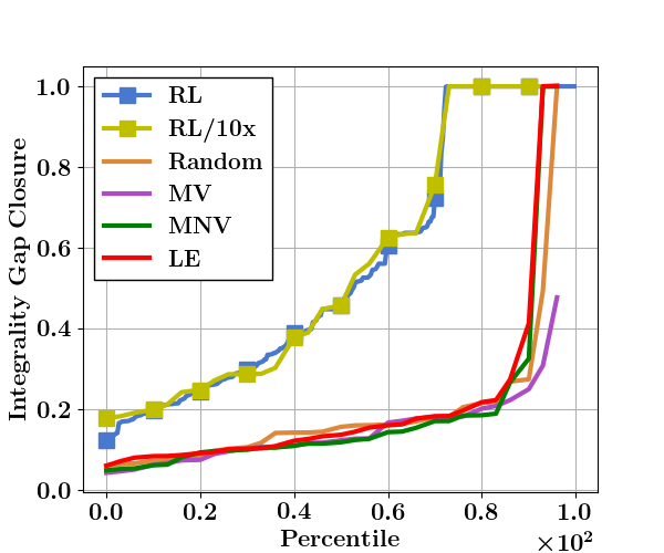
(a) Packing

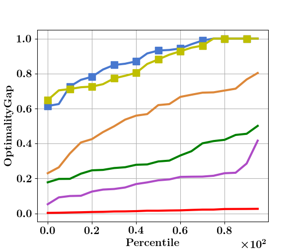
(b) Planning

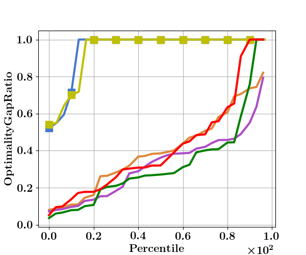
(c) Binary Packing

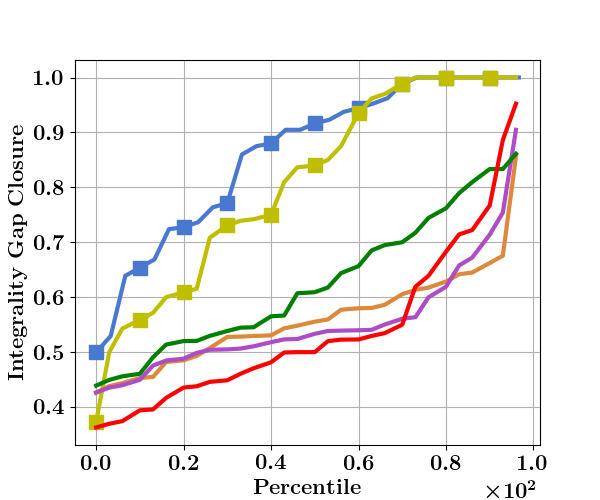
(d) Max Cut

Figure 2: Percentile plots of IGC for test instances of size roughly $1000$. X-axis shows the percentile of instances and y-axis shows the IGC achieved on adding $T=50$ cuts. Across all test instances, RL achieves significantly higher IGC than the baselines.

Experiment #2: Integrality gap closure for large-sized instances.

Next, we train and test the RL agent on significantly larger problem instances compared to the previous experiment. In the first set of experiments (Table 2 and Figure 2), we consider instances of size ($n\times m$) close to $1000$. In Table 3 and Figure 3, we report results for even larger scale problems, with instances of size close to $5000$. We add $T=50$ cuts for the first set of instances, and $T=250$ cuts for the second set of instances. However, for these instances, the cutting plane methods is unable to reach optimality. Therefore, we compare different cutting plane methods on integrality gap closed using the IGC metric defined in (2), Section 2. Table 2, 3 show that on average RL agent was able to close a significantly higher fraction of gap compared to the other methods. Figure 2, 3 provide a more detailed comparison, by showing a percentile plot – here the instances are sorted in the ascending order of IGC and then plotted in order; the $y$-axis shows the IGC and the $x$-axis shows the percentile of instances achieving that IGC. The blue curve with square markers shows the performance of our RL agent. In Figure 2, very close to the blue curve is the yellow curve (also with square marker). This yellow curve is for RL$/$10X, which is an RL agent trained on 10X smaller instances in order to evaluate generalization properties, as we describe next.

Table 3: IGC for test instances of size roughly $5000$. We show $\text{mean}\pm\text{std}$ of IGC achieved on adding $T=250$ cuts.

Tasks	Packing	Planning	Binary	Max Cut
Size	$60\times 60$	$121\times 168$	$66\times 132$	$54\times 134$
Random	$0.05\pm 0.03$	$0.38\pm 0.08$	$0.17\pm 0.12$	$0.50\pm 0.10$
MV	$0.04\pm 0.02$	$0.07\pm 0.03$	$0.19\pm 0.18$	$0.50\pm 0.06$
MNV	$0.05\pm 0.03$	$0.17\pm 0.10$	$0.19\pm 0.18$	$0.56\pm 0.11$
LE	$0.04\pm 0.02$	$0.01\pm 0.01$	$0.23\pm 0.20$	$0.45\pm 0.08$
RL	$\mathbf{0.11\pm 0.05}$	$\mathbf{0.68\pm 0.10}$	$\mathbf{0.61\pm 0.35}$	$\mathbf{0.57\pm 0.10}$

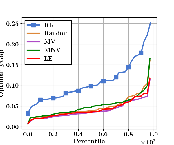
(a) Packing

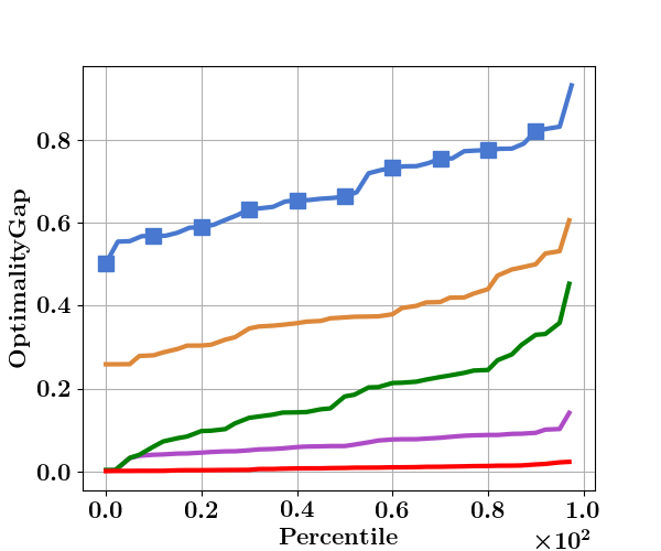
(b) Planning

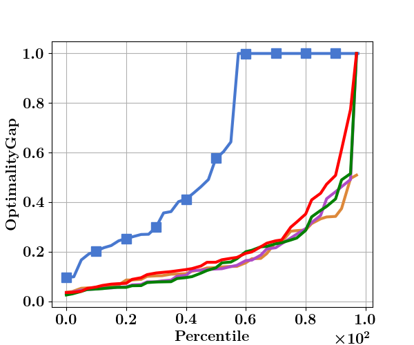
(c) Binary Packing

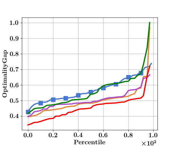
(d) Max Cut

Figure 3: Percentile plots of IGC for test instances of size roughly $5000$, $T=250$ cuts. Same set up as Figure 2 but on even larger-size instances.

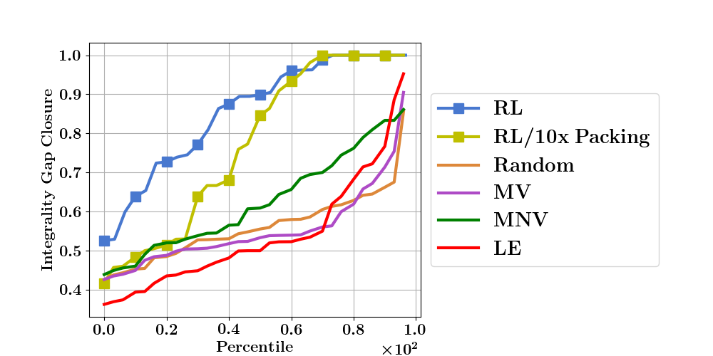
Figure 4: Percentile plots of Integrality Gap Closure. ‘RL/10X packing’ trained on instances of a completely different IP problem (packing) performs competitively on the maximum-cut instances.

Table 4: IGC in B&C. We show $\text{mean}\pm\text{std}$ across test instances.

Tasks	Packing	Planning	Binary	Max Cut
Size	$30\times 30$	$61\times 84$	$33\times 66$	$27\times 67$
No cut	$0.57\pm 0.34$	$0.35\pm 0.08$	$0.60\pm 0.24$	$1.0\pm 0.0$
Random	$0.79\pm 0.25$	$0.88\pm 0.16$	$0.97\pm 0.09$	$1.0\pm 0.0$
MV	$0.67\pm 0.38$	$0.64\pm 0.27$	$0.97\pm 0.09$	$0.97\pm 0.18$
MNV	$0.83\pm 0.23$	$0.74\pm 0.22$	$1.0\pm 0.0$	$1.0\pm 0.0$
LE	$0.80\pm 0.26$	$0.35\pm 0.08$	$0.97\pm 0.08$	$1.0\pm 0.0$
RL	$\mathbf{0.88\pm 0.23}$	$\mathbf{1.0\pm 0.0}$	$1.0\pm 0.0$	$1.0\pm 0.0$

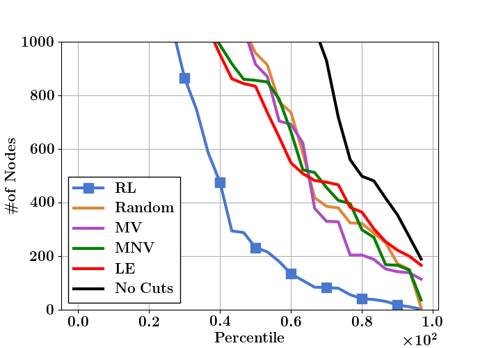
(a) Packing (1000 nodes)

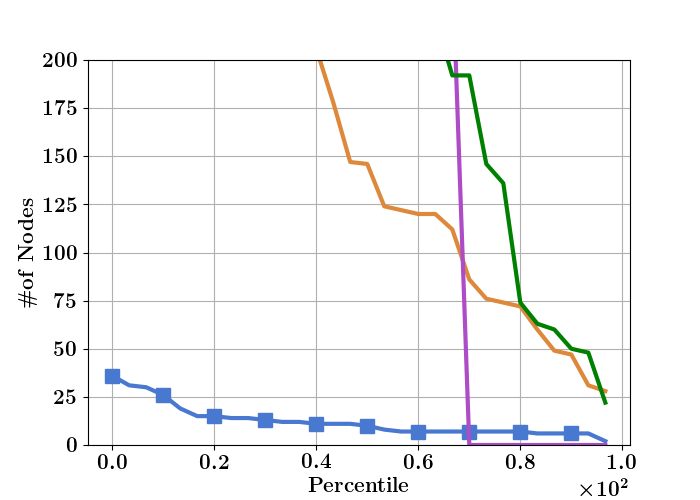
(b) Planning (200 node)

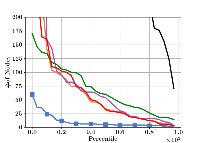
(c) Binary (200 nodes)

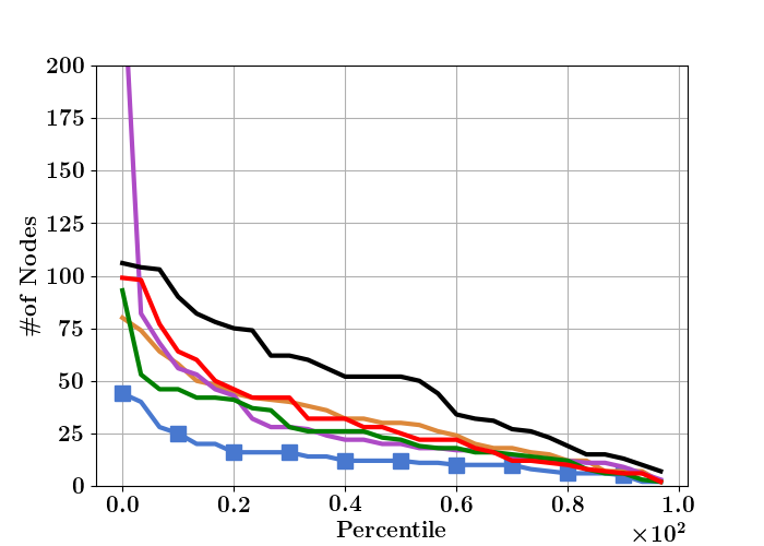
(d) Max Cut (200 nodes)

Figure 5: Percentile plots of number of B&C nodes expanded. X-axis shows the percentile of instances and y-axis shows the number of expanded nodes to close $95\%$ of the integrality gap.

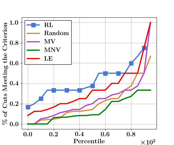
(a) Criterion 1

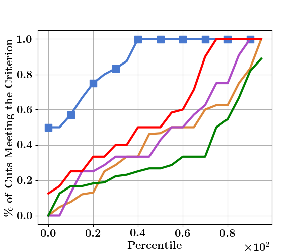
(b) Criterion 2

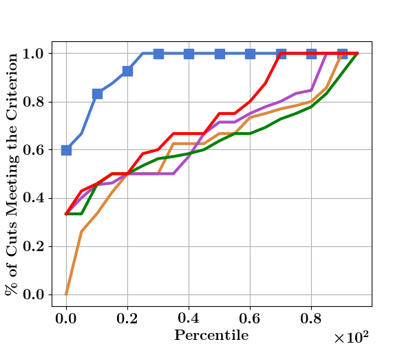
(c) Criterion 3

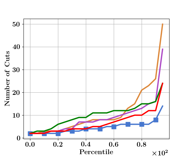
(d) Number of cuts

Figure 6: Percentage of cuts meeting the designed criteria and number of cuts on Knapsack problems. We train the RL agent on $80$ instances. All baselines are tested on $20$ instances. As seen above, RL produces consistently more ’high-quality’ cuts.

Experiment #3: Generalization.

In Figure 2, we also demonstrate the ability of the RL agent to generalize across different sizes of the IP instances. This is illustrated through the extremely competitive performance of the RL/10X agent, which is trained on 10X smaller size instances than the test instances. (Exact sizes used in the training of RL/10X agent were were $10\times 10,32\times 22,10\times 20,20\times 10$, respectively, for the four types of IP problems.) Furthermore, we test generalizability across IP classes by training an RL agent on small sized instances of the packing problem, and applying it to add cuts to $10X$ larger instances of the maximum-cut problem. The latter, being a graph optimization problem, has intuitively a very different structure from the former. Figure 4 shows that the RL/10X agent trained on packing (yellow curve) achieve a performance on larger maximum-cut instances that is comparable to the performance of agent trained on the latter class (blue curve).

Experiment #4: Impact on the efficiency of B&C.

In practice, cutting planes alone are not sufficient to solve large problems. In state-of-the-art solvers, the iterative addition of cutting planes is alternated with a branching procedure, leading to Branch-and-Cut (B&C). To demonstrate the full potential of RL, we implement a comprehensive B&C procedure but without all the additional heuristics that appear in the standard solvers. Our B&C procedure has two hyper-parameters: number of child nodes (suproblems) to expand $N_{\text{exp}}$ and number of cutting planes added to each node $N_{\text{cuts}}$. In addition, B&C is determined by the implementation of the Branching Rule, Priority Queue and Termination Condition. Further details are in the appendix.

Figure 5 gives percentile plots for the number of child nodes (suproblems) $N_{\text{exp}}$ until termination of B&C. Here, $N_{\text{cuts}}=10$ cuts were added to each node, using either RL or one of the baseline heuristics. We also include as a comparator, the B&C method without any cuts, i.e., the branch and bound method. The trained RL agent and the test instances used here are same as those in Table 2 and Figure 2. Perhaps surprisingly, the RL agent, though not designed to be used in combination with branching, shows substantial improvements in the efficiency of B&C. In the appendix, we have also included experimental results showing improvements for the instances used in Table 3 and Figure 3.

Experiment #5: Interpretability of cuts.

A knapsack problem is a binary packing problem with only one constraint. Although simple to state, these problems are NP-Hard, and have been a testbed for many algorithmic techniques, see e.g. the books (Kellerer et al., 2003; Martello and Toth, 1990). A prominent class of valid inequalities for knapsack is that of cover inequalities, that can be strengthened through the classical lifting operation (see the appendix for definitions). Those inequalities are well-studied in theory and also known to be effective in practice, see e.g. (Crowder et al., 1983; Conforti et al., 2014; Kellerer et al., 2003). Our last set of experiments gives a “reinforcement learning validation” of those cuts. We show in fact that RL, with the same reward scheme as in Experiment #2, produces many more cuts that “almost look like” lifted cover inequalities than the baselines. More precisely, we define three increasingly looser criteria for deciding when a cut is “close” to a lifted cover inequality (the plurality of criteria is due to the fact that lifted cover inequalities can be strengthened in many ways). We then check which percentage of the inequalities produced by the RL (resp. the other baselines) satisfy each of these criteria. This is reported in the first three figures in Figure 6, together with the number of cuts added before the optimal solution is reached (rightmost figure in Figure 6). More details on the experiments and a description of the three criteria are reported in the appendix. These experiments suggest that our approach could be useful to aid researchers in the discovery of strong family of cuts for IP s, and provide yet another empirical evaluation of known ones.

Runtime.

A legitimate question is whether the improvement provided by the RL agent in terms of solution accuracy comes at the cost of a large runtime. The training time for RL can indeed be significant, especially when trained on large instances. However, there is no way to compare that with the human-designed heuristics. In testing, we observe no significant differences in time required by an RL policy to choose a cut vs. time taken to execute a heuristic rule. We detail the runtime comparison in the appendix.

5 Conclusions

We presented a deep RL approach to automatically learn an effective cutting plane strategy for solving IP instances. The RL algorithm learns by trying to solve a pool of (randomly generated) training instances again and again, without having access to any solved instances. The variety of tasks across which the RL agent is demonstrated to generalize without being trained for, provides evidence that it is able to learn an intelligent algorithm for selecting cutting planes. We believe our empirical results are a convincing step forward towards the integration of ML techniques in IP solvers. This may lead to a functional answer to the “Hamletic question Branch-and-cut designers often have to face: to cut or not to cut?” (Dey and Molinaro, 2018).

Acknowledgements.

Author Shipra Agrawal acknowledges support from an Amazon Faculty Research Award.

Appendix A Experiment Details

A.1 Projection into the original variable space

In the following we look at only the first iteration of the cutting plane procedure, and we drop the iteration index $t$. Recall the LP relaxation of the original IP problem (1), where $A\in\mathbb{Q}^{m\times n},b\in\mathbb{Q}^{m}$:

$$\left\{\begin{array}[]{ll}\min c^{T}x\\ Ax\leq b\\ x\geq 0.\end{array}\right.$$

When a simplex algorithm solves the LP, the original LP is first converted to a standard form where all inequalities are transformed into equalities by introducing slack variables.

$$\left\{\begin{array}[]{ll}\min c^{T}x\\ Ax+\mathbb{I}s=b\\ x\geq 0,s\geq 0,\end{array}\right.$$ (6)

where $\mathbb{I}$ is an identity matrix and $s$ is the set of slack variables. The simplex method carries out iteratively operations on the tableau formed by $[A,\mathbb{I}],b$ and $c$. At convergence, the simplex method returns a final optimal tableau. We generate a Gomory’s cut using the row of the tableau that corresponds to a fractional variable of the optimal solution $x_{\text{LP}}^{\ast}$. This will in general create a cutting plane of the following form

$$e^{T}x+r^{T}s\leq d$$ (7)

where $e,x\in\mathbb{R}^{n},r,s\in\mathbb{R}^{m}$ and $d\in\mathbb{R}$. Though this cutting plane involves slack variables, we can get rid of the slack variables by multiplying both sides of the linear constraints in (6) by $r$

$$r^{T}Ax+r^{T}s=r^{T}b$$ (8)

and subtract the new cutting plane (7) by the above. This leads to an equivalent cutting plane

$$(e^{T}-r^{T}A)x\leq d-r^{T}b.$$ (9)

Note that this cutting plane only contains variables in the original variable space. For a downstream neural network that takes in the parameters of the cutting planes as inputs, we find it helpful to remove such slack variables. Slack variables do not contribute to new information regarding the polytope and we can also parameterize a network with a smaller number of parameters.

A.2 Integer programming formulations of benchmark problems

A wide range of benchmark instances can be cast into special cases of IP problems. We provide their specific formulations below. For simplicity, we only provide their general IP formulations (with $\leq,\geq,=$ constraints). It is always possible to convert original formulations into the standard formulation (1) with properly chosen $A,b,c,x$. Some problems are formulated within a graph $G=(V,E)$ with nodes $v\in V$ and edges $(v,u)\in E$.

Their formulations are as follows:

Max Cut.

We have one variable per edge $y_{u,v},(u,v)\in E$ and one variable per node $x_{u},u\in V$. Let $w_{u,v}\geq 0$ be a set of non-negative weights per edge.

$$\left\{\begin{array}[]{ll}\max\sum_{(u,v)\in E}w_{uv}y_{uv}\\ y_{uv}\leq x_{u}+x_{v},\forall(u,v)\in E\\ y_{uv}\leq 2-x_{u}-x_{v},\forall(u,v)\in E\\ 0\leq x,y\leq 1\\ x_{u},y_{uv}\in\mathbb{Z}\quad\forall u\in V,(u,v)\in E.\end{array}\right.$$ (10)

In our experiments the graphs are randomly generated. To be specific, we specify a vertex size $|V|$ and edge size $|E|$. We then sample $|E|$ edges from all the possible $|V|\cdot(|V|-1)/2$ edges to form the final graph. The weights $w_{uv}$ are uniformly sampled as an integer from $0$ to $10$. When generating the instances, we sample graphs such that $|V|,|E|$ are of a particular size. For example, for middle size problem we set $|V|=7,|E|=20$.

Packing.

The packing problem takes the generic form of (1) while requiring that all the coefficients of $A,b,c$ be non-negative, in order to enforce proper resource constraints.

Here the constraint coefficients $a_{ij}$ for the $j$th variable and $i$th constraint is sampled as an integer uniformly from $0$ and $5$. Then the RHS coefficient $b_{i}$ is sampled from $9n$ to $10n$ uniformly as an integer where $n$ is the number of variables. Each component of $c_{j}$ is uniformly sampled as an integer from $1$ to $10$.

Binary Packing.

Binary packing augments the original packing problem by a set of binary constraints on each variable $x_{i}\leq 1$.

Here the constraint coefficients $a_{ij}$ for the $j$th variable and $i$th constraint is sampled as an integer uniformly from $5$ and $30$. Then the RHS coefficient $b_{i}$ is sampled from $10n$ to $20n$ uniformly as an integer where $n$ is the number of variables. Each component of $c_{j}$ is uniformly sampled as an integer from $1$ to $10$.

Production Planning.

Consider a production planning problem (Pochet and Wolsey, 2006) with time horizon $T$. The decision variables are production $x_{i},1\leq i\leq T$, along with by produce / not produce variables $y_{i},1\leq i\leq T$ and storage variables $s_{i},0\leq i\leq T$. Costs $p_{i}^{\prime},h_{i}^{\prime},q_{i}$ and demands $d_{i}$ are given as problem parameters. The LP formulation is as follows

$$\left\{\begin{array}[]{ll}\min\sum_{i=1}^{T}p_{i}^{\prime}x_{i}+\sum_{i=0}^{T}h_{i}^{\prime}s_{i}+\sum_{i=0}^{T}q_{i}y_{i}\\ s_{i-1}+x_{i}=d_{i}+s_{i},\forall 1\leq i\leq T\\ x_{i}\leq My_{i},\forall 1\leq i\leq T\\ s\geq 0,x\geq 0,0\leq y\leq 1\\ s_{0}=s_{0}^{\ast},s_{T}=s_{T}^{\ast}\\ x,s,y\in\mathbb{Z}^{T},\end{array}\right.$$ (11)

where $M$ is a positive large number and $s_{0}^{\ast},s_{T}^{\ast}$ are also given.

The instance parameters are the initial storage $s_{0}^{\ast}=0$, final storage $s_{T}^{\ast}=20$ and big $M=100$. The revenue parameter $p_{i}^{\prime},h_{i}^{\prime},q_{i}$ are generated uniformly random as integers from $1$ to $10$.

Size of IP formulations.

In our results, we describe the sizes of the IP instances as $n\times m$ where $n$ is the number of columns and $m$ is the number of rows of the constraint matrix $A$ from the LR of (1). For a packing problem with $n$ items and $m$ resource constraints, the IP formulation has $n$ variables and $m$ constraints; for planning with period $K$, $n=3K+1$, $m=4K+1$; for binary packing, there are $n$ extra binary constraints compared to the packing problem; for max-cut, the problem is defined on a graph with a vertex set $V$ and an edge set $V$, and its IP formulation consists of $n=|V|+|E|$ variables and $m=3|E|+|V|$ constraints.

A.3 Criteria for selecting Gomory cuts

Recall that $I_{t}$ is the number of candidate Gomory cuts available in round $t$, and $i_{t}$ denotes the index of cut chosen by a given baseline. The baseline heuristics we use are the following:

• Random. One cut $i_{t}\sim\text{Uniform}\{1,2...I_{t}\}$ is chosen uniformly at random from all the candidate cuts.

• Max Violation (MV). Let $x_{B}^{\ast}(t)$ be the basic feasible solution of the curent LP relaxation. MV selects the cut that corresponds to the most fractional component, i.e. $i_{t}=\arg\max\{|[x_{B}^{\ast}(t)]_{i}-\text{round}([x_{B}^{\ast}(t)]_{i})|\}$.

• Max Normalized Violation (MNV). Recall that $\tilde{A}$ denotes the optimal tableau obtained by the simplex algorithm upon convergence. Let $\tilde{A}_{i}$ be the $i$th row of $\tilde{A}$. Then, MNV selects cut $i_{t}=\arg\max\{|[x_{B}^{\ast}(t)]_{i}-\text{round}([x_{B}^{\ast}(t)]_{i})|/\|\tilde{A}_{i}\|\}$.

• Lexicographic (LE): Add the cutting plane with the least index, i.e. $i_{t}=\arg\min\{i,[x_{B}^{\ast}(t)]_{i}\text{ is fractional}\}$.

The first three rules are common in the IP literature, see e.g. (Wesselmann and Stuhl, 2012), while the fourth is the original rule used by Gomory to prove the convergence of his method (Gomory, 1960).

A.4 Hyper-parameters

Policy architecture.

The policy network is implemented with Chainer (Tokui et al., 2015). The attention embedding $F_{\theta}$ is a 2-layer neural network with $64$ units per layer and tanh activation. The LSTM network encodes variable sized inputs into hidden vector with dimension $10$.

During a forward pass, a LSTM $+$ Attention policy will take the instance, carry out embedding into a $n$-d vector and then apply attention. Such architecture allows for generalization to variable sized instances (different number of variables). We apply such architecture in the generalization part of the experiments.

On the other hand, a policy network can also consist of a single attention network. This policy can only process IP instances of a fixed size (fixed number of varibles) and cannot generalize to other sizes. We apply such architecture in the IGC part of the experiments.

ES optimization.

Across all experiments, we apply Adam optimizer (Kingma and Ba, 2014) with learning rate $\alpha=0.01$ to optimize the policy network. The perturbation standard deviation $\sigma$ is selected from $\{0.002,0.02,0.2\}$. By default, we apply $N=10$ perturbations to construct the policy gradient for each iteration, though we find that $N=1$ could also work as well. For all problem types except planning, we find that $\sigma=0.2$ generally works properly except for planning, where we apply $\sigma=0.02$ and generate $N=5$ trajectory per instance per iteration. Empirically, we observe that the training is stable for both policy architectures and the training performance converges in $\leq 500$ weight updates.

Distributed setup.

For training, we use a Linux machine with 60 virtual CPUs. To fully utilize the compute power of the machine, the trajectory collection is distributed across multiple workers, which run in parallel.

Appendix B Branch-and-Cut Details

As mentioned in the introduction, Branch-and-Cut (B&C) is an algorithmic procedure used for solving IP problems. The choice of which variable to branch on, as well as which node of the branching tree to explore next, is the subject of much research. In our experiments, we implemented a B&C with very simple rules, as explained below. This is motivated by the fact that our goal is to evaluate the quality of the cutting planes added by the RL rather than obtaining a fast B&C method. Hence, sophisticated and computationally expensive branching rules could have overshadowed the impact of cutting planes. Instead, simple rules (applied both to the RL and to the other techniques) highlight the impact of cutting planes for this important downstream application.

We list next several critical elements of our implementation of B&C.

Branching rule.

At each node, we branch on the most fractional variable of the corresponding LP optimal solution ($0.5$ being the most fractional).

Priority queue.

We adopt a FIFO queue (Breath first search). FIFO queue allows the B&C procedure to improve the lower bound.

Termination condition.

Let $z_{0}=c^{T}x_{\text{LP}}^{\ast}(0)$ be the objective of the initial LP relaxation. As B&C proceeds, the procedure finds an increasing set of feasible integer solutions $\mathcal{X}_{F}$, and an upper bound on the optimal objective $z^{\ast}=c^{T}x_{\text{IP}}^{\ast}$ is $z_{\text{upper}}=\min_{x\in\mathcal{X}_{F}}c^{T}x$. Hence, $z_{\text{upper}}$ monotonically decreases.

Along with B&C, cutting planes can iteratively improve the lower bound $z_{\text{lower}}$ of the optimal objective $z^{\ast}$. Let $z_{i}$ be the objective of the LP solution at node $i$ and denote $\mathcal{N}$ as the set of unpruned nodes with unexpanded child nodes. The lower bound is computed as $z_{\text{lower}}=\min_{i\in\mathcal{N}}z_{i}$ and monotonically increases as the B&C procedure proceeds.

This produces a ratio statistic

$$r=\frac{z_{\text{upper}}-z_{\text{lower}}}{z_{\text{upper}}-z^{*}_{\text{LP}}}>0$$

Note that since $z_{\text{lower}}\geq z^{*}_{\text{LP}}$, $z_{\text{lower}}$ monotonically increases, and $z_{\text{upper}}$ monotonically decreases, $r$ monotonically decreases. The B&C terminates when $r$ is below some threshold which we set to be $0.0001$.

Appendix C Test Time Considerations

Stopping criterion.

Though at training time we guide the agent to generate aggressive cuts that tighten the LP relaxation as much as possible, the agent can exploit the defects in the simulation environment - numerical errors, and generate invalid cuts which cut off the optimal solution.

This is undesirable in practice. In certain cases at test time, when we execute the trained policy, we adopt a stopping criterion which automatically determines if the agent should stop adding cuts, in order to prevent from invalid cuts. In particular, at each iteration let $r_{t}=|c^{T}x_{\text{LP}^{\ast}(t)}-c^{T}x_{\text{LP}^{\ast}(t+1)}|$ be the objective gap achieved by adding the most recent cut. We maintain a cumulative ratio statistics such that

$$s_{t}=\frac{r_{t}}{\sum_{t^{\prime}\leq t}r_{t}}.$$

We terminate the cutting plane procedure once the average $s_{t}$ over a fixed window of size $H$ is lower than certain threshold $\eta$. In practice, we set $H=5,\eta=0.001$ and find this work effectively for all problems, eliminating all the numerical errors observed in reported tasks. Intuitively, this approach dictates that we terminate the cutting plane procedure once the newly added cuts do not generate significant improvements for a period of $H$ steps.

To analyze the effect of $\eta$ and $H$, we note that when $H$ is too small or $\eta$ is too large, we have very conservative cutting plane procedure. On the other hand when $H$ is large while $\eta$ is small, the cutting plane procedure becomes more aggressive.

Greedy action.

The policy network defines a stochastic policy, i.e. a categorical distribution over candidate cuts. At test time, we find taking the greedy action $i^{\ast}=\arg\max p_{i}$ to be more effective in certain cases, where $p_{i}$ is the categorical distribution over candidate cuts. The justification for this practice is that: the ES optimization procedure can be interpreted as searching for a parameter $\theta$ such that the induced distribution over trajectories has large concentration on those high return trajectories. Given a trained model, to decode the most likely trajectory of horizon $T$ generated by the policy, we need to run a full tree search of depth $T$, which is infeasible in practice. Taking the greedy action is equivalent to applying a greedy strategy in decoding the most likely trajectory.

This approach is highly related to beam search in sequence modeling (Sutskever et al., 2014) where the goal is to decode the prediction that the model assigns the most likelihood to. The greedy action selection above corresponds to a beam search with $1$-step lookahead.

Appendix D Details on the Interpretation of Cutts

One interesting aspect of studying the RL approach to generating cuts, is to investigate if we can interpret cuts generated by RL. For a particular class of IP problems, certain cuts might be considered as generally ’better’ than other cuts. For example, these cuts might be more effective in terms of closing the objective gap, according to domain knowledge studied in prior literature. Ideally, we would like to find out what RL has learned, whether it has learned to select these more ’effective’ cuts with features identified by prior works. Here, we focus on Knapsack problems.

Problem instances.

Consider the knapsack problems

$$\left\{\begin{array}[]{ll}\max\sum_{i}^{n}c_{i}x_{i}\\ \sum_{i=1}^{n}a_{i}x_{i}\leq\beta:=\sum_{i=1}^{n}a_{i}/2\\ x_{i}\in\{0,1\},\\ \end{array}\right.$$ (12)

where $a_{i}$ are generated independently and uniformly in $[1,30]$ as integers, and the $c_{i}$ are generated independently and uniformly in $[1,10]$. We consider $n=10$ in our experiments. Knapsack problems are fundamental in IP, see e.g. (Kellerer et al., 2003). The intuition of the problem is that we attempt to pack as many items as possible into the knapsack, as to maximize the profit of the selected items. Polytopes as (12) are also used to prove strong (i.e., quadratic) lower bounds on the Chvátal-Gomory rank of polytopes with $0/1$ vertices (Rothvoß and Sanità, 2017).

Evaluation scores.

For knapsack problems, one effective class of cuts is given by cover inequalities, and their strengthening through lifting (Conforti et al., 2014; Kellerer et al., 2003). The cover inequality associated to a set $S\subseteq\{1,\dots,n\}$ with $\sum_{i\in S}a_{i}>\beta$ and $|S|=k$ is given by

$$\sum_{i\in S}x_{i}\leq k-1.$$

Note that cover inequalities are valid for (12). The inequality can be strengthened (while maintaining validity) by replacing the $0$ coefficients of variables $x_{i}$ for $i\in\{1,\dots,n\}\setminus S$ with appropriate positive coefficients, leading to the lifted cover inequality below:

$$\sum_{i\in S}x_{i}+\sum_{\notin S}\alpha_{i}x_{i}\leq k-1.$$ (13)

with all $\alpha_{i}\geq 0$. There are in general exponentially many ways to generate lifted cover inequalities from a single cover inequality. In practice, further strengthenings are possible, for instance, by perturbing the right-hand side or the coefficients of $x_{i}$ for $i\in S$. We provide three criteria for identifying (strengthening of) lifted cover inequalities, each capturing certain features of the inequalities (below, RHS denotes the right-hand side of a given inequality).

• There exists an integer $p$ such that (1) the RHS is an integer multiple of $p$ and (2) $p$ times (number of variable with coefficient exactly $p$) $>$ RHS.

Criterion 1 is satisfied by all lifted cover inequalities as in (13). The scaling by $p$ is due to the fact that an inequality may be scaled by a positive factor, without changing the set of points satisfying it.

• There exists an integer $p$ such that (1) holds and (2’) $p$ times (number of variables with coefficients between $p$ and $p+2$) $>$ RHS.

• There exists an integer $p$ such that (1) holds and (2”) p times (number of variables with coefficients at least $p$) $>$ RHS.

A lifted cover inequality can often by strengthened by increasing the coefficients of variables in $S$, after the lifting has been performed. We capture this by criteria 2 and 3 above, where $2$ is a stricter criterion, as we only allow those variables to have their coefficients increased by a small amount.

For each cut $c_{j}$ generated by the baseline (e.g. RL), we evaluate if this cut satisfies the aforementioned conditions. For one particular condition, if satisfied, the cut is given a score $s(c_{j})=1$ or else $s(c_{j})=0$. On any particular instance, the overall score is computed as an average across the $m$ cuts that are generated to solve the problem with the cutting plane method:

$$\frac{1}{m}\sum_{j=1}^{m}s(c_{j})\in[0,1].$$

Evaluation setup.

We train a RL agent on $100$ knapsack instances and evaluate the scores on another independently generated set of $20$ instances. Please see the main text for the evaluation results.

Appendix E Additional results on Large-scale Instances

We provide additional results on large-scale instances in Figure 7, in the context of B&C. Experimental setups and details are similar to those of the main text: we set the threshold limit to be $1000$ nodes for all problem classes. The results show the percentile plots of the number of nodes required to achieve a certain level of IGC during the B&C with the use of cutting plane heuristics, where the percentile is calculated across instances. Baseline results for each baseline are shown via curves in different colors. When certain curves do not show up in the plot, this implies that these heuristics do not achieve the specified level of IGC within the node budgets. The IGC level is set to be $95$% as in the main text, except for the random packing problem where it is set to be $25$%.

The IGC of the random packing is set at a relatively low level because random packing problems are significantly more difficult to solve when instances are large-scaled. This is consistent with the observations in the main text.

Overall, we find that the performance of RL agent significantly exceeds that of the other baseline heuristics. For example, on the planning problem, other heuristics barely achieve the IGC within the node budgets. There are also cases where RL does similarly to certain heuristics, such as to MNV on the Max Cut problems.

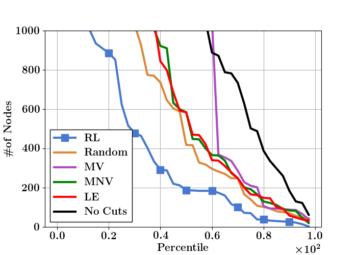
(a) Packing (25% IGC, 1000 nodes)

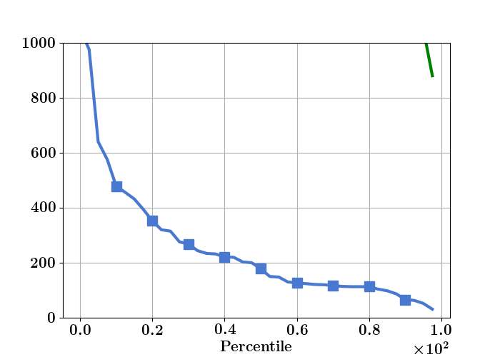
(b) Planning (95% IGC, 1000 nodes)

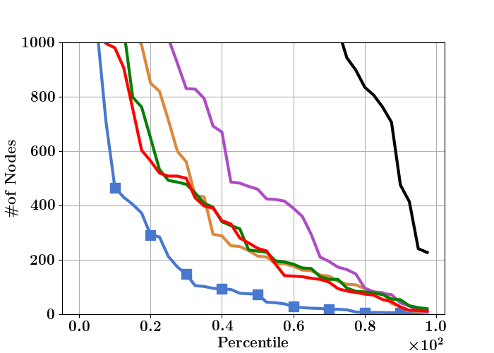
(c) Binary Packing (95% IGC, 1000 nodes)

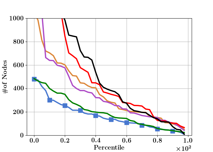
(d) Max Cut (95% IGC, 1000 nodes)

Figure 7: Percentile plots of number of B&C nodes expanded for large-scale instances. The same setup as Figure 5 but for even larger instances.

Table 5: IGC in B&C with large-scale instances. We adopt the same setup as Table 2

Tasks	Packing	Planning	Binary	Max Cut
Size	$60\times 60$	$122\times 168$	$66\times 132$	$54\times 134$
No cut	$0.26\pm 0.09$	$0.25\pm 0.04$	$0.74\pm 0.24$	$0.95\pm 0.09$
Random	$0.31\pm 0.08$	$0.65\pm 0.10$	$0.94\pm 0.10$	$0.99\pm 0.04$
MV	$0.23\pm 0.08$	$0.27\pm 0.07$	$0.92\pm 0.12$	$0.98\pm 0.06$
MNV	$0.27\pm 0.08$	$0.33\pm 0.15$	$0.93\pm 0.10$	$1.0\pm 0.0$
LE	$0.28\pm 0.08$	$0.25\pm 0.04$	$0.95\pm 0.08$	$0.95\pm 0.09$
RL	$\mathbf{0.36\pm 0.10}$	$\mathbf{0.99\pm 0.02}$	$\mathbf{0.96\pm 0.08}$	$1.0\pm 0.0$

Appendix F Comparison of Distributed Agent Interface

To scale RL training to powerful computational architecture, it is imperative that the agent becomes distributed. Indeed, recent years have witnessed an increasing attention on the design and implementation of distributed algorithms (Mnih et al., 2016; Salimans et al., 2017; Espeholt et al., 2018; Kapturowski et al., 2018).

General distributed algorithms adopt a learner-actor architecture, i.e. one central learner and multiple distributed actors. Actors collect data and send partial trajectories to the learner. The learner takes data from all actors and generates updates to the central parameter. The general interface requires a function $\pi_{\theta}(a|s)$ parameterized by $\theta$, which takes a state $s$ and outputs an action $a$ (or a distribution over actions). In a gradient-based algorithm (e.g. (Espeholt et al., 2018)), the actor executes such an interface with the forward mode and generates trajectory tuple $(s,a)$; the learner executes the interface with the backward mode to compute gradients and update $\theta$. Below we list several practical considerations why ES is a potentially better distributed alternative to such gradient-based distributed algorithms in this specific context, where state/action spaces are irregular.

• Communication. The data communication between learner-actor is more complex for general gradient-based algorithms. Indeed, actors need to send partial trajectories $\{(s_{i},a_{i},r_{i})\}_{i=1}^{\tau}$ to the learner, which requires careful adaptations to cases where the state/action space are irregular. On the other hand, ES only require sending returns over trajectories $\sum_{i=0}^{T}r_{i}$, which greatly simplifies the interface from an engineering perspective.

• Updates. Gradient-based updates require both forward/backward mode of the agent interface. Further, the backward mode function needs to be updated such that batched processing is efficient to allow for fast updates. For irregular state/action space, this requires heavier engineering because of e.g. arrays of variable sizes are not straightforward to be batched. On the other hand, ES only requires forward mode computations required by CPU actors.

Appendix G Considerations on CPU Runtime

In practice, instead of the number of cuts, a more meaningful budget constraint on solvers is the CPU runtime, i.e. practitioners typically set a runtime constraint on the solver and expect the solver to return the best possible solution within this constraint. Below, we report runtime results for training/test time. We will show that even under runtime constraints, the RL policy achieves significant performance gains.

Training time.

During training time, it is not straightforward to explicitly maintain a constraint on the runtime, because it is very sensitive to hardware conditions (e.g. number of available processors). Indeed, prior works (Khalil et al., 2016; Dai et al., 2017) do not apply runtime constraint during training time, though runtime constraint is an important measure at test time.

The absolute training time depends on specific hardware architecture. In our experiments we train with a single server with $64$ virtual CPUs. Recall that each update consists in collecting trajectories across training instances and generating one single gradient update. We observe that typically the convergence takes place in $\leq 500$ weight updates (iterations).

Test time.

To account for the practical effect of runtime, we need to account for the following trade-off: though RL based policy produces higher-quality cutting planes in general, running the policy at test time could be costly. To characterize the trade-offs, we address the following question: (1) When adding a fixed number of cuts, does RL lead to higher runtime? (2) When solving a particular problem, does RL lead to performance gains in terms of runtime?

To address (1), we reuse the experiments in Experiment #2, i.e. adding a fixed number of cuts $T=50$ on middle sized problems. The runtime results are presented in Table 6, where we show that RL cutting plane selection does not increase the runtime significantly compared to other ’fast’ heuristics. Indeed, RL increases the average runtime in some cases while decreases in others. Intuitively, we expect the runtime gains to come from the fact that RL requires a smaller number of cuts - leading to fewer iterations of the algorithm. However, this is rare in Experiment #2, where for most instances optimal solution is not reached in maximum number of cuts, so all heuristics and RL add same number of cuts ($T=50$). We expect such advantages to become more significant with the increase of the size of the problem, as the computational gain of adding good cuts becomes more relevant. We confirm such intuitions from the following.

To address (2), we reuse the results from Experiment #4, where we solve more difficult instances with B&C, we report the runtime results in Table 7. In these cases, the benefits of high-quality cuts are magnified by a decreased number of iterations (i.e. expanded nodes) - indeed, for RL policy, the advantages resulting from decreased iterations significantly overweight the potentially slight drawbacks of per-iteration runtime. In Table 7, we see that RL generally requires much smaller runtime than other heuristics, mainly due to a much smaller number of B&C iterations. Note that these results are consistent with Figure 5. Again, for large-scale problems, this is an important advantage in terms of usage of memory and overall performance of the system.

Table 6: CPU runtime for adding cutting planes (units are seconds). Here we present the results from Experiment #2 from the main text, where we fix the number of added cuts $T=50$. Note that though RL might increase runtime in certain cases, it achieves much larger IGC within the cut budgets. Note that these results are consistent with Table 2.

Tasks	Packing	Planning	Binary	Max Cut
Size	$30\times 30$	$61\times 84$	$33\times 66$	$27\times 67$
Random	$0.06\pm 0.01$	$0.09\pm 0.01$	$0.088\pm 0.003$	$0.08\pm 0.01$
MV	$0.9\pm 0.01$	$0.100\pm 0.004$	$0.10\pm 0.01$	$0.11\pm 0.01$
MNV	$0.10\pm 0.02$	$0.100\pm 0.004$	$0.12\pm 0.02$	$0.12\pm 0.01$%
RL	$0.10\pm 0.02$	$0.14\pm 0.03$	$0.07\pm 0.04$	$0.08\pm 0.02$

Table 7: CPU runtime in B&C with large-scale instances. The measures are normalized with respect to RL so that the RL runtime is always measured as $100$%. Here, we measure the runtime as the time it takes to reach a certain level of IGC. We only measure the runtime on test instances where the IGC level is reached within the node budgets. When the IGC is not reached for most test instances (as in the case of the planning problem for most baselines), the runtime measure is ’N/A’. Note that the results here are consistent with Table 3 and Figure 7.

Tasks	Packing	Planning	Binary	Max Cut
Size	$60\times 60$	$122\times 168$	$66\times 132$	$54\times 134$
Random	$146\%$	N/A	$190\%$	$250$%
MV	$256\%$	N/A	$340\%$	$210$%
MNV	$238\%$	N/A	$370\%$	$\mathbf{95}$%
LE	$120\%$	N/A	$370$%	$120$%
RL	$\mathbf{100\%}$	$\mathbf{100\%}$	$\mathbf{100\%}$	$100\%$

References

- Balas et al. (1993) Balas, E., Ceria, S., and Cornuéjols, G. (1993). A lift-and-project cutting plane algorithm for mixed 0–1 programs. Mathematical programming, 58(1-3):295–324.
- Balcan et al. (2018) Balcan, M.-F., Dick, T., Sandholm, T., and Vitercik, E. (2018). Learning to branch. arXiv preprint arXiv:1803.10150.
- Bello et al. (2017) Bello, I., Pham, H., Le, Q. V., Norouzi, M., and Bengio, S. (2017). Neural combinatorial optimization.
- Bengio et al. (2018) Bengio, Y., Lodi, A., and Prouvost, A. (2018). Machine learning for combinatorial optimization: a methodological tour d’horizon. arXiv preprint arXiv:1811.06128.
- Bixby (2017) Bixby, B. (2017). Optimization: past, present, future. Plenary talk at INFORMS Annual Meeting.
- Conforti et al. (2014) Conforti, M., Cornuéjols, G., and Zambelli, G. (2014). Integer programming, volume 271. Springer.
- Cornuéjols et al. (2013) Cornuéjols, G., Margot, F., and Nannicini, G. (2013). On the safety of gomory cut generators. Math. Program. Comput., 5(4):345–395.
- Crowder et al. (1983) Crowder, H., Johnson, E. L., and Padberg, M. (1983). Solving large-scale zero-one linear programming problems. Operations Research, 31(5):803–834.
- Dai et al. (2017) Dai, H., Khalil, E. B., Zhang, Y., Dilkina, B., and Song, L. (2017). Learning combinatorial optimization algorithms over graphs. arXiv preprint arXiv:1704.01665.
- Dantzig et al. (1954) Dantzig, G., Fulkerson, R., and Johnson, S. (1954). Solution of a large-scale traveling-salesman problem. Journal of the operations research society of America, 2(4):393–410.
- Dey and Molinaro (2018) Dey, S. S. and Molinaro, M. (2018). Theoretical challenges towards cutting-plane selection. Mathematical Programming, 170(1):237–266.
- Espeholt et al. (2018) Espeholt, L., Soyer, H., Munos, R., Simonyan, K., Mnih, V., Ward, T., Doron, Y., Firoiu, V., Harley, T., Dunning, I., et al. (2018). Impala: Scalable distributed deep-rl with importance weighted actor-learner architectures. arXiv preprint arXiv:1802.01561.
- Gomory (1960) Gomory, R. (1960). An algorithm for the mixed integer problem. Technical report, RAND CORP SANTA MONICA CA.
- Gurobi Optimization (2015) Gurobi Optimization, I. (2015). Gurobi optimizer reference manual. URL http://www. gurobi. com.
- Hochreiter and Schmidhuber (1997) Hochreiter, S. and Schmidhuber, J. (1997). Long short-term memory. Neural computation, 9(8):1735–1780.
- Kapturowski et al. (2018) Kapturowski, S., Ostrovski, G., Quan, J., Munos, R., and Dabney, W. (2018). Recurrent experience replay in distributed reinforcement learning.
- Kellerer et al. (2003) Kellerer, H., Pferschy, U., and Pisinger, D. (2003). Knapsack problems. 2004.
- Khalil et al. (2017) Khalil, E., Dai, H., Zhang, Y., Dilkina, B., and Song, L. (2017). Learning combinatorial optimization algorithms over graphs. In Advances in Neural Information Processing Systems, pages 6348–6358.
- Khalil et al. (2016) Khalil, E. B., Le Bodic, P., Song, L., Nemhauser, G. L., and Dilkina, B. N. (2016). Learning to branch in mixed integer programming. In AAAI, pages 724–731.
- Kingma and Ba (2014) Kingma, D. P. and Ba, J. (2014). Adam: A method for stochastic optimization. arXiv preprint arXiv:1412.6980.
- Kool and Welling (2018) Kool, W. and Welling, M. (2018). Attention solves your tsp. arXiv preprint arXiv:1803.08475.
- Li et al. (2018) Li, Z., Chen, Q., and Koltun, V. (2018). Combinatorial optimization with graph convolutional networks and guided tree search. In Advances in Neural Information Processing Systems, pages 539–548.
- Martello and Toth (1990) Martello, S. and Toth, P. (1990). Knapsack problems: algorithms and computer implementations. Wiley-Interscience series in discrete mathematics and optimiza tion.
- Mnih et al. (2016) Mnih, V., Badia, A. P., Mirza, M., Graves, A., Lillicrap, T., Harley, T., Silver, D., and Kavukcuoglu, K. (2016). Asynchronous methods for deep reinforcement learning. In International conference on machine learning, pages 1928–1937.
- Nowak et al. (2017) Nowak, A., Villar, S., Bandeira, A. S., and Bruna, J. (2017). A note on learning algorithms for quadratic assignment with graph neural networks. arXiv preprint arXiv:1706.07450.
- Pochet and Wolsey (2006) Pochet, Y. and Wolsey, L. A. (2006). Production planning by mixed integer programming. Springer Science & Business Media.
- Rothvoß and Sanità (2017) Rothvoß, T. and Sanità, L. (2017). 0/1 polytopes with quadratic chvátal rank. Operations Research, 65(1):212–220.
- Salimans et al. (2017) Salimans, T., Ho, J., Chen, X., Sidor, S., and Sutskever, I. (2017). Evolution strategies as a scalable alternative to reinforcement learning. arXiv preprint arXiv:1703.03864.
- Sutskever et al. (2014) Sutskever, I., Vinyals, O., and Le, Q. V. (2014). Sequence to sequence learning with neural networks. In Advances in neural information processing systems, pages 3104–3112.
- Tokui et al. (2015) Tokui, S., Oono, K., Hido, S., and Clayton, J. (2015). Chainer: a next-generation open source framework for deep learning. In Proceedings of workshop on machine learning systems (LearningSys) in the twenty-ninth annual conference on neural information processing systems (NIPS), volume 5, pages 1–6.
- Vaswani et al. (2017) Vaswani, A., Shazeer, N., Parmar, N., Uszkoreit, J., Jones, L., Gomez, A. N., Kaiser, Ł., and Polosukhin, I. (2017). Attention is all you need. In Advances in neural information processing systems, pages 5998–6008.
- Vinyals et al. (2015) Vinyals, O., Fortunato, M., and Jaitly, N. (2015). Pointer networks. In Advances in Neural Information Processing Systems, pages 2692–2700.
- Wesselmann and Stuhl (2012) Wesselmann, F. and Stuhl, U. (2012). Implementing cutting plane management and selection techniques. Technical report, Tech. rep., University of Paderborn.