A monotone data augmentation algorithm for longitudinal data analysis via multivariate skew-t, skew-normal or t distributions

Abstract

The mixed effects model for repeated measures (MMRM) has been widely used for the analysis of longitudinal clinical data collected at a number of fixed time points. We propose a robust extension of the MMRM for skewed and heavy-tailed data on basis of the multivariate skew-t distribution, and it includes the multivariate normal, t, and skew-normal distributions as special cases. An efficient Markov chain Monte Carlo algorithm is developed using the monotone data augmentation and parameter expansion techniques. We employ the algorithm to perform controlled pattern imputations for sensitivity analyses of longitudinal clinical trials with nonignorable dropouts. The proposed methods are illustrated by real data analyses. Sample SAS programs for the analyses are provided in the online supplementary material.

1 Introduction

The mixed effects model for repeated measures (MMRM) has been commonly used for the primary analysis of longitudinal continuous outcomes in clinical trials aiddiqui:2009 ; mallinckrodt:2008 . As recommended by the regulatory guidelines e9:1999 ; chmp:2015 , the main analysis in clinical trials shall be unambiguously prespecified in the protocol. For this reason, the observations within a subject are usually assumed to follow a multivariate normal distribution with an unstructured covariance matrix in MMRM aiddiqui:2009 ; mallinckrodt:2008 ; laird:1987 ; tang:2017sim . If the covariance structure is misspecified, the treatment effect estimate may be biased in the presence of missing data lu:2010 , and the test for the fixed effects may not be able to control the type I error rate gurka:2011 ; gadda:2007 . A covariance selection approach using Akaike’s information criterion or Schwarz’s Bayesian information criterion also tends to inflate the type I error rate gomez:2005 .

The controlled imputation methodology little:1996 ; 2013:carpenter ; 2013:mallinckrodta ; 2017:tangb has become increasingly popular in sensitivity analyses of longitudinal trials with nonignorable dropouts. The controlled imputation and MMRM assume the same observed data distribution, but specify different mechanisms for missingness due to dropout. The MMRM assumes the data are missing at random (MAR rubin:1976 ). It implies that subjects who discontinue the treatment early have the same mean response profiles as subjects who complete the trial. The MAR mechanism may not be convincing if the dropout is due to adverse events or inadequate efficacy. Sensitivity analyses under missing not at random (MNAR rubin:1976 ) are recommended by recent regulatory guidelines ich:2017 ; chmp:2010 and a FDA-mandated panel report from the National Research Council NRC:2010 . Under MNAR, the response profiles differ systematically between dropouts and completers. In the controlled imputation, the mean outcomes among subjects in the experimental arm after dropout are assumed to be similar to that of control subjects, or get worse compared to subjects who stay on the treatment. The assumption is clinically plausible and easy to understand. If the treatment effect remains significant in a conservative nonignorable sensitivity analysis, we can claim the robustness of the primary conclusion obtained under MAR.

The controlled imputation specifies a pattern mixture model (PMM little:1993 ) for the longitudinal outcomes in the sense that their joint distribution depends on the dropout time. The controlled imputation is generally implemented via multiple imputation (MI), and this will be explained in Section 7. Tang 2017:tangb ; 2017:tanga introduces a formal Markov chain Monte Carlo (MCMC) algorithm to conduct the controlled imputation based on the monotone data augmentation (MDA) strategy. It extends and improves Schafer’s schafer:1997 MDA algorithm for multivariate normal outcomes. The algorithm is unaffected by the dropout mechanism. The missing data after dropout are integrated out of the posterior distribution, and imputed after the algorithm converges. Only the intermittent missing outcomes and the model parameters are drawn iteratively before the Markov chain reaches its stationary distribution. It imputes fewer missing values, and tends to converge faster with smaller autocorrelation between posterior samples than an algorithm that imputes all missing outcomes in each iteration schafer:1997 ; 2017:tanga . Tang 2018:tangd ; tang:2019 develops the controlled imputation for longitudinal outcomes with potentially different types of variables based on the factored likelihood, in which the conditional model of the outcome at each visit given the outcomes at previous visits can be linear, binary logistic, multinomial logistic, proportional odds, Poisson, negative binomial, skew-normal (SN AZZALINI:1985 ) or skew-t (ST azzalini:2003 ) regressions, and may vary by visits.

The main purpose of this article is to extend the controlled imputation to non-normal longitudinal continuous outcomes. In the mixed effects model, inference about the fixed effects is asymptotically valid for non-normal outcomes verbeke:1997 , but may suffer from some loss of efficiency pinheiro:2001 ; zhang:2001 in large samples. The inference is vulnerable to severe departures from normality in small and moderate samples arnau:2013 , and this can be easily understood in the simple case of a t test boos:2000 . Furthermore, imputing skewed outcomes under normality leads to biased MI estimates of the distributional shape parameters hippel:2013 . We relax the normality assumption in MMRM by modeling the within subject dependence using the multivariate ST distributionazzalini:2003 , which includes the multivariate SNazzalini:1996 , normal and t distributions as special cases. This extension is different from our previous work tang:2019 , where the data are modeled by a sequence of univariate ST regressions.

The SN and ST distributions have a roughly bell-shaped density, and can be made arbitrarily close to the normal or t density by regulating suitable parameters azzalini:2003 . They are also capable of accommodate asymmetry and heavy tails often exhibited in clinical data liu:1995 ; jara:2008 ; lachos:2009 . In the SN and ST distributions, the skewness is partially induced by truncating some latent variables arnold:2002 ; valle:2006 . Such selection or truncation mechanisms arise naturally in clinical studies. For example, a clinical trial may enroll only patients whose disease severity is above a certain level. In Section 2, we briefly review the univariate and multivariate SN and ST distributions, and derive the relevant conditional distribution.

The SN and ST distributions present some undesirable properties in statistical inference liseo:2006 ; bayes:2007 ; branco:2013 . This can be illustrated in the univariate regression. In the scalar case, the asymptotic distribution of the maximum likelihood estimate (MLE) is bimodal when the distribution of the data is close to normal, and there is a non-negligible chance that the MLE of the skewness parameter can be infinite for skewed data pewsey:2000 ; Arellano:2008 . Similar issues exist in Bayesian inference liseo:2006 ; liseo:2013 . In general, the likelihood function changes slowly at large values of the skewness and/or degrees of freedom (df) parameters, and converges to a constant when the skewness and/or df parameters reach their limit values (all other parameters are fixed). As a result, the posterior distribution in Bayesian inference may be improper under a diffuse prior, and the posterior estimates of the skewness and/or df parameters can be sensitive to the decay rate of their marginal prior densities liu:1995 ; liseo:2006 ; Fonseca:2008 . The problems become even more complex in the multivariate case. Section 3.1 investigates how to specify the priors for the skewness, df and covariance parameters to address the inference challenges mentioned above.

In Sections 3.2 and 4, we extend Tang’s MDA algorithm 2017:tangb ; 2017:tanga to the multivariate ST, SN and t regressions. The underlying idea is to reorganize these robust regressions as the normal linear regression with the introduction of some latent variables. The parameter expansion (PX liu:1999 ; liu:2000 ) and block sampling techniques are employed to improve the mixing and accelerate the convergence of the Markov chain. Section 5 applies the MDA algorithm to the controlled imputation. The proposed MDA algorithm and missing data imputation methods are illustrated by real data analyses in Section 6.

Throughout the article, the following notations will be used. Let $\mathcal{G}(a,b)$ denote a gamma distribution with shape $a$, rate $b$ and mean $a/b$. Let $N(\bm{\mu},\Omega)$ denote the normal distribution with mean $\bm{\mu}$ and covariance $\Omega$, and $t(\bm{\mu},\Omega,\nu)$ the $t$ distribution with $\nu$ df. In the multivariate case, $\bm{\mu}$ is a vector and $\Omega$ is a square matrix. The probability density functions (PDF) of the gamma, normal and t distributions are denoted, respectively, by $\mathcal{G}(\cdot|\cdot)$, $N(\cdot|\cdot)$ and $t(\cdot|\cdot)$. Let $\Phi(\cdot)$ and $T_{\nu}(\cdot)$ denote respectively the cumulative distribution function (CDF) of $N(0,1)$ and $t(0,1,\nu)$. Let $N^{+}(\mu,\sigma^{2})$ be the scalar positive normal distribution left truncated at $0$, and $t^{+}(\mu,\sigma^{2},\nu)$ the scalar positive t distribution. Let $\text{W}^{-1}(A,n_{0})$ denote the inverse Wishart distribution with PDF $\pi(\Sigma)\propto|A|^{n_{0}/2}|\Sigma|^{-(n_{0}+p+1)/2}\exp[-\text{tr}(A\Sigma^{-1})/2]$.

2 Review of univariate and multivariate SN and ST distributions

We review the univariate and multivariate SN and ST distributions introduced by Azzalini and his collaborators AZZALINI:1985 ; azzalini:1996 ; azzalini:2003 . We focus on their convolution-type stochastic representation azzalini:2003 ; lee:2013a as it allows straightforward interpretation of the skewness parameters in the multivariate distribution (see Section 2.2 below), and makes it easier to design the MCMC algorithm schnatter:2010 . An alternative stochastic representation is given by Azzalini and Capitanio azzalini:2003 . In both representations, the skewness is induced by truncating a latent variable arnold:2002 . Such mechanism arises naturally in practice. For example, in clinical trials, patients may be selected only if a variable of interest is above a threshold.

2.1 Univariate SN and ST distributions

The PDF of a SN AZZALINI:1985 random variable $y\sim\mathcal{SN}(\mu,\sigma^{2},\psi)$ is given by $2N(y|\mu,\omega^{2})\Phi[\lambda(y-u)/\omega]$, where $\omega^{2}=\sigma^{2}+\psi^{2}$. It can be stochastically represented as

$$y=\mu+\psi\text{\small$\mathcal{W}$}+\epsilon,$$

where $\mu$ is the location parameter, $\text{\small$\mathcal{W}$}\sim N^{+}(0,1)$ is independent of $\epsilon\sim N(0,\sigma^{2})$, and $\lambda=\psi/\sigma$ is the skewness parameter. Its mean is $\text{E}(y)=\mu+\psi\sqrt{\frac{2}{\pi}}$.

The parameter $\lambda$ controls the degree to which the data depart from normality. When $\lambda=0$, the SN distribution reduces to the normal distribution. The degree of the skewness of $y$ increases as the absolute value of $\lambda$ increases. Since the maximum skewness and kurtosis are $0.995$ and $0.869$ respectively AZZALINI:1985 , the SN distribution is suitable only for mildly or moderately non-normal data.

The ST distributionazzalini:2003 allows a higher degree of skewness and kurtosis. A ST random variable $y\sim\mathcal{ST}(\mu,\sigma^{2},\psi,\nu)$ can be stochastically represented as

$$y=\mu+\frac{1}{\sqrt{d}}[\psi\text{\small$\mathcal{W}$}^{*}+\epsilon]=\mu+\psi\text{\small$\mathcal{W}$}+\frac{1}{\sqrt{d}}\epsilon,$$ (1)

where $d\sim\chi_{\nu}^{2}/\nu$ [i.e. $d\sim\mathcal{G}(\nu/2,\nu/2)$], $\text{\small$\mathcal{W}$}^{*}\sim N^{+}(0,1)$, $\text{\small$\mathcal{W}$}=\text{\small$\mathcal{W}$}^{*}/\sqrt{d}\sim t^{+}(0,1,\nu)$ and $\epsilon\sim N(0,\sigma^{2})$. We get $\text{E}(y)=\mu+\psi\sqrt{\frac{\nu}{\pi}}\frac{\Gamma((\nu-1)/2)}{\Gamma(\nu/2)}$, where $\Gamma(\cdot)$ is the gamma function. The PDF of $y$ is given by

$$f_{{}_{\mathcal{ST}}}(y|\mu,\omega^{2},\lambda,\nu)=2t(y|\mu,\omega^{2},\nu)\,T_{\nu+1}\left[\lambda\frac{y-\mu}{\omega}\sqrt{\frac{\nu+p}{\nu+\frac{(y-\mu)^{2}}{\omega^{2}}}}\right].$$ (2)

2.2 Multivariate SN and ST distributions

A multivariate version of the SN distribution is introduced by Azzalini and Dalla Valle azzalini:1996 . The random vector $\bm{y}=(y_{1},\ldots,y_{p})^{\prime}\sim\mathcal{SN}(\bm{\mu},\Sigma,\bm{\psi})$ can be represented as schnatter:2010

$$(y_{1},\ldots,y_{p})^{\prime}=\bm{\mu}+\bm{\psi}\text{\small$\mathcal{W}$}+\bm{\epsilon}$$ (3)

where $\bm{\epsilon}=(\epsilon_{1},\ldots,\epsilon_{p})^{\prime}\sim N(\bm{0},\Sigma)$, $\text{\small$\mathcal{W}$}\sim N^{+}(0,1)$, $\bm{\mu}=(\mu_{1},\ldots,\mu_{p})^{\prime}$ is a vector containing the location parameters, and $\bm{\psi}=(\psi_{1},\ldots,\psi_{p})^{\prime}$ is a vector of skewness parameters. The PDF of $\bm{y}$ is given by

$$f_{{}_{\mathcal{SN}}}(\bm{y}|\bm{\mu},\Sigma,\bm{\psi})=2N(\bm{y}|\bm{\mu},\Omega)\Phi[\bm{\lambda}^{*^{\prime}}(\bm{y}-\bm{\mu})]=2N(\bm{y}|\bm{\mu},\Omega)\Phi\left[\sum_{j=1}^{p}\lambda_{j}\frac{y_{j}-\mu_{j}}{\omega_{j}}\right],$$ (4)

where $\omega_{j}^{2}$ is the $(j,j)$th element of $\Omega=\Sigma+\bm{\psi}\bm{\psi}^{\prime}$, and $\bm{\lambda}^{*}=\left(\frac{\lambda_{1}}{\omega_{1}},\ldots,\frac{\lambda_{p}}{\omega_{p}}\right)=\frac{\Omega^{-1}\bm{\psi}}{\sqrt{1-\bm{\psi}^{\prime}\Omega^{-1}\bm{\psi}}}=\frac{\Sigma^{-1}\bm{\psi}}{\sqrt{1+\bm{\psi}^{\prime}\Sigma^{-1}\bm{\psi}}}$.

The multivariate SN distribution azzalini:1996 was originally introduced through the parametrization $(\bm{\mu},\lambda_{1},\ldots,\lambda_{p},\Omega)$. It is difficult to interpret the skewness parameter $\lambda_{j}$, which does not provide information about the skewness of $y_{j}$, not even on its sign Arellano:2008 . Also, $\Omega$ is not the covariance matrix of $\bm{y}$. Let $\Sigma_{jj}=\text{var}(\epsilon_{j})$. By the stochastic representation (3), the marginal distribution of $y_{j}=\mu_{j}+\psi_{j}\text{\small$\mathcal{W}$}+\epsilon_{j}$ is $SN(\mu_{j},\Sigma_{jj},\psi_{j})$, and its skewness is controlled by $\psi_{j}/\sqrt{\Sigma_{jj}}$.

The multivariate ST distribution azzalini:2003 $\bm{y}\sim\mathcal{ST}(\bm{\mu},\Sigma,\bm{\psi},\nu)$ can be represented as

$$(y_{1},\ldots,y_{p})^{\prime}=\bm{\mu}+\bm{\psi}\text{\small$\mathcal{W}$}+\frac{1}{\sqrt{d}}\bm{\epsilon},$$ (5)

where $d\sim\chi_{\nu}^{2}/\nu$, $\text{\small$\mathcal{W}$}^{*}\sim N^{+}(0,1)$ and $\text{\small$\mathcal{W}$}=\text{\small$\mathcal{W}$}^{*}/\sqrt{d}\sim t^{+}(0,1,\nu)$. The PDF of $\bm{y}$ is

$$f_{{}_{\mathcal{ST}}}(\bm{y}|\bm{\mu},\Sigma,\bm{\psi},\nu)=2t(\bm{y}|\bm{\mu},\Omega,\nu)T_{\nu+p}\left[\bm{\lambda}^{*^{\prime}}(\bm{y}-\bm{\mu})\sqrt{\frac{\nu+p}{\nu+(\bm{y}-\bm{\mu})^{\prime}\Omega^{-1}(\bm{y}-\bm{\mu})}}\,\right].$$ (6)

Let the LDL decomposition of $\Sigma$ be denoted by $\Sigma=L\Lambda L^{\prime}$, where $\Lambda=\text{diag}(\gamma_{1}^{-1},\ldots,\gamma_{p}^{-1})$, $L=U^{-1}$, and $U=$ $\begin{bmatrix}1&0&\ldots&0\\ -\beta_{21}&1&\ldots&0\\ -\beta_{p1}&\ldots&-\beta_{p,p-1}&1\\ \end{bmatrix}$. Equation (5) can be reorganized as $U\bm{y}=U\bm{\mu}+U\bm{\psi}\text{\small$\mathcal{W}$}+\frac{1}{\sqrt{d}}U\bm{\epsilon}$ or equivalently as

$$y_{j}=\sum_{t=1}^{j-1}\beta_{jt}y_{t}+\underline{\mu}_{j}+\underline{\psi}_{j}\text{\small$\mathcal{W}$}+\frac{\varepsilon_{j}}{\sqrt{d}}\text{ for }j=1,\ldots,p,$$ (7)

where $(\underline{\mu}_{j},\underline{\psi}_{j})=(\mu_{j},\psi_{j})-\sum_{t=1}^{j-1}\beta_{jt}(\mu_{t},\psi_{t})$, and $\varepsilon_{j}$’s are independently distributed as $\varepsilon_{j}\sim N(0,\gamma_{j}^{-1})$.

It is well known azzalini:1996 ; azzalini:2003 that the conditional distribution of $\bm{y}_{s_{2}}=(y_{s+1},\ldots,y_{p})^{\prime}$ given $\bm{y}_{s_{1}}=(y_{1},\ldots,y_{s})^{\prime}$ is no longer the SN/ST distribution. As shown in Lemma 1 below, the conditional distribution of $\bm{y}_{s_{2}}$ given $\bm{y}_{s_{1}}$ can be expressed similarly to Equation (7) except that the location parameter for the positive normal or t random variable is not $0$. We omit the proof since a more general result is given in Appendix A.1.1.

Lemma 1.

(a) The conditional distribution of $(d,\text{\small$\mathcal{W}$})$ given $\bm{y}_{s_{1}}=(y_{1},\ldots,y_{s})^{\prime}$ is

$$\begin{aligned} \text{\small$\mathcal{W}$}|y_{1},\ldots,y_{s}\sim t^{+}\left[\frac{B}{A},\frac{\nu_{d}}{A(\nu+s)},\nu+s\right]\,\text{ and }\,\\ d|\text{\small$\mathcal{W}$},y_{1},\ldots,y_{s}\sim\mathcal{G}\left[\frac{\nu+s+1}{2},\frac{\nu_{d}+A(\text{\small$\mathcal{W}$}-\frac{B}{A})^{2}}{2}\right],\end{aligned}$$ (8)

where $y_{j}^{*}=y_{j}-\sum_{t=1}^{j-1}\beta_{jt}y_{t}-\underline{\mu}_{j}$, $A=1+\sum_{j=1}^{s}\gamma_{j}\underline{\psi}_{j}^{2}$, $B=\sum_{j=1}^{s}\gamma_{j}\underline{\psi}_{j}y_{j}^{*}$ and $\nu_{d}=\nu+\sum_{j=1}^{s}\gamma_{j}y_{j}^{*^{2}}-B^{2}/A$.
(b) The conditional distribution of $\bm{y}_{s_{2}}$ given $\bm{y}_{s_{1}}$ can be represented as a sequence of univariate conditional distributions

$$y_{j}=\sum_{t=1}^{j-1}\beta_{jt}y_{t}+\underline{\mu}_{j}+\underline{\psi}_{j}\text{\small$\mathcal{W}$}_{s}+\frac{1}{\sqrt{d_{s}}}\varepsilon_{j}\,\text{ for }\,j\geq s+1,$$

where $\varepsilon_{k}\sim N(0,\gamma_{k}^{-1})$, $\varepsilon_{k}$’s are independent, and $(\text{\small$\mathcal{W}$}_{s},d_{s})$ is the random sample from the conditional distribution (8).
(c) The conditional distribution of $\bm{y}_{s_{2}}$ given $\bm{y}_{s_{1}}$ can be equivalently represented in matrix form as

$$\begin{aligned} \begin{bmatrix}y_{s+1}\\ \ldots\\ y_{p}\end{bmatrix}=\begin{bmatrix}\mu_{s+1}\\ \ldots\\ \mu_{p}\end{bmatrix}-U_{s_{22}}^{-1}U_{s_{12}}\begin{bmatrix}y_{1}-\mu_{1}\\ \ldots\\ y_{s}-\mu_{s}\end{bmatrix}+U_{s_{22}}^{-1}\begin{bmatrix}\underline{\psi}_{s+1}\\ \ldots\\ \underline{\psi}_{p}\end{bmatrix}\text{\small$\mathcal{W}$}_{s}+\frac{U_{s_{22}}^{-1}}{\sqrt{d_{s}}}\begin{bmatrix}\varepsilon_{s+1}\\ \ldots\\ \varepsilon_{p}\end{bmatrix},\end{aligned}$$

where $\begin{bmatrix}U_{s_{11}}&\bm{0}\\ U_{s_{21}}&U_{s_{22}}\\ \end{bmatrix}=$ $\left[\begin{array}[]{ccc|cc}1&0&0&\ldots&0\\ \ldots&&&&\\ -\beta_{s1}&\ldots&1&\ldots&0\\ \hline\cr\ldots&&\ldots&\ldots&0\\ -\beta_{p1}&\ldots&-\beta_{ps}&\ldots&1\\ \end{array}\right]$ is a partition of $U$.

Notes:

1. In Lemma 1(a), the conditional distribution of $d$ given $y_{1},\ldots,y_{s}$ is not gamma due to the constraint $\text{\small$\mathcal{W}$}>0$.
2. Lemma 1 can be applied to the multivariate SN distribution by setting $\nu\equiv\infty$, $d\equiv 1$ and $\text{\small$\mathcal{W}$}|\bm{y}_{s_{1}}\sim N^{+}(\frac{B}{A},\frac{1}{A})$.
3. In the multivariate t distribution ($\psi_{j}\equiv 0$), the conditional distribution of $\bm{y}_{s_{2}}$ given $\bm{y}_{s_{1}}$ can be written as $y_{j}=\sum_{t=1}^{j-1}\beta_{jt}y_{t}+\underline{\mu}_{j}+\frac{\varepsilon_{j}}{\sqrt{d_{s}}}$ for $j>s$, where $d_{s}\sim\frac{\chi_{\nu+s}^{2}}{\nu+\sum_{t=1}^{s}\gamma_{t}y_{t}^{*^{2}}}$.
4. The skewness of the conditional distribution of $y_{s+1}$ given $y_{1},\ldots,y_{s}$ is a monotone function of $\underline{\psi}_{j}\sqrt{\gamma_{j}}$.

3 MDA algorithm for MMRM with no restriction on fixed effects

Suppose a study consists of $n_{tot}$ subjects, and the data are collected at $p$ fixed time points. Let $\bm{y}_{i}=(y_{i1},\ldots,y_{ip})^{\prime}$ denote the complete outcome for subject $i$. In general, $\bm{y}_{i}$’s won’t be fully observed. Let $s_{i}$ be the last visit that subject $i$ has a measurement observed, and $s_{i}=0$ if the subject has no observed outcome. Let $\bm{y}_{io}$, $\bm{y}_{im}$ and $\bm{y}_{iw}$ denote respectively the observed data with $o_{i}$ elements, intermittent missing data with $m_{i}=s_{i}-o_{i}$ elements prior to dropout, and missing data after dropout for subject $i$. Without loss of generality, we sort the data so that subjects in pattern $s$ are arranged before subjects in pattern $t$ if $s>t$. Let $n_{j}$ be the total number of subjects in patterns $j,\ldots,p$. Let $n=n_{1}$ be the number of subjects with at least one observed outcome.

The following MMRM is often used to analyze longitudinal outcomes collected at a number of fixed time points aiddiqui:2009 ; laird:1987

$$y_{ij}=\sum_{k=1}^{q}\alpha_{kj}x_{ik}+\xi_{ij}\text{ for }j=1,\ldots,p,$$ (9)

where $i=1,\ldots,n_{tot}$ indexes subjects, $q$ is the number of baseline covariates, $\alpha_{kj}$ is the effect of covariate $x_{ik}$ at visit $j$, and $\bm{\xi}_{i}=(\xi_{i1},\ldots,\xi_{ip})^{\prime}\sim N(0,\Omega)$. Let $x_{i1}\equiv 1$ if the model contains an intercept term. In clinical trials, we set the treatment status as $x_{iq}=g_{i}=1$ for the experimental treatment, and $g_{i}=0$ for the control treatment. We place no constraints on the covariate effects $\alpha_{kj}$’s, and they can vary freely over time. As discussed in Section 1, we employ an unstructured covariance matrix. It generally provides a good control of the type I error rate under the null hypothesis, and results in a negligible loss in efficiencylu:2010 under the alternative hypothesis when compared to the analysis based on the true covariance structure (it is difficult to be prespecified) in moderate to large samples. A structured covariance matrix, which may be induced through the use of random effects, is useful when individuals have a large number of observations, or varying times of observations laird:1987 .

Model (9) assumes that the outcomes are normally distributed. Inference about the treatment effect based on the normality assumption can be inefficient in the presence of outliers pinheiro:2001 ; zhang:2001 , and may be invalid for highly non-normal data particularly when the sample size is small arnau:2013 . In this article, we use the multivariate t, SN or ST distribution to model skewed and/or fat-tailed data. Model (9) will be denoted respectively by MMRM-n, MMRM-t, MMRM-sn or MMRM-st when the residual errors $\bm{\xi}_{i}=(\xi_{i1},\ldots,\xi_{ip})^{\prime}$ are modeled by the multivariate normal, t, SN or ST distribution.

By introducing the latent variables $(d_{i},\text{\small$\mathcal{W}$}_{i})$, we can expand the MMRM-st as

$$y_{ij}=\sum_{k=1}^{q}\alpha_{kj}x_{ik}+\psi_{j}\text{\small$\mathcal{W}$}_{i}+\frac{1}{\sqrt{d_{i}}}\epsilon_{ij}=\sum_{k=1}^{\text{\tiny{$Q$}}}\alpha_{kj}x_{ik}+\frac{1}{\sqrt{d_{i}}}\epsilon_{ij},$$ (10)

where $d_{i}\sim\mathcal{G}(\nu/2,\nu/2)$, $\text{\small$\mathcal{W}$}_{i}^{*}\sim N^{+}(0,1)$, $\text{\small$\mathcal{W}$}_{i}=\text{\small$\mathcal{W}$}_{i}^{*}/\sqrt{d_{i}}$, $\text{\small{$Q$}}=q+1$, $\alpha_{\text{\tiny{$Q$}}j}=\psi_{j}$, and $x_{i\text{\tiny{$Q$}}}=\text{\small$\mathcal{W}$}_{i}$. The MMRM-sn and MMRM-t can be obtained by setting $d_{i}\equiv 1$ (i.e. $\nu\equiv\infty$) and $\psi_{j}\equiv 0$ respectively in model (10).

Model (10) can be reorganized as the product of the following conditional models

$$y_{ij}\sim N\left(\sum_{k=1}^{\text{\tiny{$Q$}}}\underline{\alpha}_{kj}x_{ik}+\sum_{t=1}^{j-1}\beta_{jt}y_{it},(d_{i}\gamma_{j})^{-1}\right)\text{ for }j=1,\ldots,p,$$ (11)

where $\underline{\alpha}_{kj}=\alpha_{kj}-\sum_{t=1}^{j-1}\beta_{jt}\alpha_{kt}$. Note that $\underline{\alpha}_{\text{\tiny{$Q$}}j}=\underline{\psi}_{j}=\psi_{j}-\sum_{t=1}^{j-1}\beta_{jt}\psi_{t}$.

3.1 The prior distribution

We assume that $\nu$ and $(\Sigma,\bm{\alpha},\underline{\psi}_{1},\ldots,\underline{\psi}_{p})$ are independent, and that $\bm{\alpha},\underline{\psi}_{1},\ldots,\underline{\psi}_{p}$ are conditionally independent given $\Sigma$ in the prior distribution, where $\bm{\alpha}=\begin{bmatrix}\alpha_{11}&\ldots&\alpha_{q1}\\ &\ldots&\\ \alpha_{1p}&\ldots&\alpha_{qp}\end{bmatrix}$. We use noninformative or objective priors in our numerical examples, but our specification allows informative priors. The missing data imputation is based on model (11) with the parameterization $\{\nu,(\bm{\theta}_{1},\gamma_{1}),\ldots,(\bm{\theta}_{p},\gamma_{p})\}$, where $\bm{\theta}_{j}=(\underline{\alpha}_{1j},\ldots,\underline{\alpha}_{\text{\tiny{$Q$}}j},\beta_{j1},\ldots,\beta_{jj-1})^{\prime}$. The prior on $(\bm{\theta}_{j},\gamma_{j})$’s can be induced from the prior on $(\Sigma,\bm{\alpha},\underline{\psi}_{1},\ldots,\underline{\psi}_{p})$. It is also possible to place priors directly on $(\bm{\theta}_{j},\gamma_{j})$’s.

3.1.1 Prior on $\Sigma$

We employ the hierarchical prior introduced by Huang and Wand huang:2013

$$\rho_{j}\stackrel{{\scriptstyle i.i.d}}{{\sim}}\mathcal{G}\left(\frac{1}{2},\frac{1}{a_{0}^{2}}\right)\text{ and }\Sigma|\rho_{1},\ldots,\rho_{p}\sim\text{W}^{-1}(A_{w},n_{w}),$$

where $n_{w}=n_{0}+p-1$, $A_{w}=2n_{0}\,\text{diag}(\rho_{1},\ldots,\rho_{p})$. It is an extension of the half-t prior gelman:2006 used in a hierarchical model of variance parameters. The choice of $n_{0}=2$ and a large value for $a_{0}$ (e.g. $a_{0}=10^{5}$) corresponds to highly noninformative half-t priors on each standard deviation term and uniform priors on each correlation termhuang:2013 .

The inverse Wishart distribution $\text{W}^{-1}(A_{w},n_{w})$ with fixed $A_{w}$ and $n_{w}$ is commonly used as the prior for $\Sigma$ in the multivariate normal and t linear regressions liu:1995 ; schafer:1997 ; 2015a:tang . It reduces to Jeffrey’s prior at $n_{w}=0$ and $A_{w}=\bm{0}$. The inverse Wishart or Jeffrey’s prior can be quite informative or inappropriate in the multivariate SN and ST regression for highly skewed data, and the argument is the same as that in the univariate regression tang:2019 .

3.1.2 Prior on the skewness parameters

In the scalar case, the Bayes estimate of the skewness parameter $\lambda=\psi\sqrt{\gamma}$ can be infinite under a diffuse prior since there is a non-negligible chance that the likelihood function is a monotone function of $\lambda$ at fixed $(\mu,\omega^{2})$. The issue can be resolved by using the objective prior for $\lambda$ liseo:2006 ; bayes:2007 . The prior has no closed-form expression, but can be well approximated liseo:2006 ; branco:2013 by $\lambda\sim t(0,\pi^{2}/4,1/2)$, or equivalently by $\psi|\gamma\sim t(0,\pi^{2}/4\gamma,1/2)$. No appropriate objective prior has been developed in the multivariate case branco:2013 . We set the prior $\underline{\psi}_{j}|\Sigma\sim t(0,\pi^{2}/4\gamma_{j},1/2)$ for the skewness parameter $\underline{\psi}_{j}$ of $\underline{y}_{ij}$, and assume $\underline{\psi}_{j}$’s are conditionally independent given $\Sigma$ in the prior. The prior is equivalent to the following hierarchical prior

$$d_{j_{\text{\tiny$\psi$}}}\sim\mathcal{G}\left(\frac{1}{4},\frac{1}{4}\right)\text{ and }\underline{\psi}_{j}|\Sigma,d_{j_{\text{\tiny$\psi$}}}\sim N\left(0,\frac{\pi^{2}}{4d_{j_{\text{\tiny$\psi$}}}\gamma_{j}}\right)\text{ for }j=1,\ldots,p.$$

Liseo and Parisi liseo:2013 specifies a prior that requires certain constraints on the skewness parameters $\psi_{j}$’s to make $\Omega$ positive definite liseo:2013 , and assumes conditional independence among the skewness parameters $\psi_{j}$’s for $y_{ij}$’s given $\Sigma$. Our prior is more convenient to use, and might be more reasonable since $\underline{y}_{ij}$’s tend to be less correlated than $y_{ij}$’s.

3.1.3 Prior on $\bm{\alpha}$

Suppose the prior for $\bm{\alpha}$ is

$$\text{vec}(\bm{\alpha})|\Sigma\sim N(\text{vec}(\bm{\alpha}_{0}),M^{+}\otimes\Sigma),$$

where $M$ is a given $q\times q$ covariance matrix with rank $r^{*}$, and $M^{+}$ is the Moore-Penrose inverse of $M$. We allow $M$ to be degenerate 2015a:tang . If all elements in the $k$-th column of $\bm{\alpha}_{0}$, and all elements in the $k$-th row and $k$-th column of $M$ are $0$, the prior for the effects $(\alpha_{k1},\ldots,\alpha_{kp})$ of covariate $x_{ik}$ is flat. We set $M=\bm{0}$ and $\bm{\alpha}_{0}=\bm{0}$ in our examples.

3.1.4 Prior on $($$\bm{\theta}$${}_{j},\gamma_{j})$’s

The prior on $(\bm{\theta}_{1},\gamma_{1},\ldots,\bm{\theta}_{p},\gamma_{p})$ can be induced from the prior on $(\bm{\alpha},\underline{\psi}_{1},\ldots,\underline{\psi}_{p},\Sigma)$. By Lemma $2$ of Tang 2015a:tang , we get

$$\begin{aligned} d_{j_{\text{\tiny$\psi$}}}\sim\mathcal{G}(1/4,1/4)\text{ and }\pi(\theta_{j},\gamma_{j})\propto\gamma_{j}^{\frac{n_{w}+2j+r-p-1}{2}-1}\exp\left[-\frac{\gamma_{j}}{2}\tilde{\bm{\theta}}_{j}^{\prime}E_{j}\tilde{\bm{\theta}}_{j}\right]\end{aligned}$$ (12)

for $j=1,\ldots,p$, where $\tilde{\bm{\theta}}_{j}=(-\bm{\theta}_{j}^{\prime},1)^{\prime}$, $E=\begin{bmatrix}M&\bm{0}&M\bm{\alpha}_{0}^{\prime}\\ \bm{0}^{\prime}&\frac{4d_{j_{\text{\tiny$\psi$}}}}{\pi^{2}}&\bm{0}^{\prime}\\ \bm{\alpha}_{0}M&\bm{0}&\bm{\alpha}_{0}M\bm{\alpha}_{0}^{\prime}+A_{w}\\ \end{bmatrix}$ is a $(\text{\small{$Q$}}+p)\times(\text{\small{$Q$}}+p)$ matrix, $E_{j}$ is the $(\text{\small{$Q$}}+j)\times(\text{\small{$Q$}}+j)$ leading principle submatrix of $E$, and $r=r^{*}+1$ is the rank of the matrix $\text{diag}(M,\frac{4d_{j_{\text{\tiny$\psi$}}}}{\pi^{2}})$. Since $\bm{\alpha}_{0}=\bm{0}$ and $M=\bm{0}$, we get $r^{*}=0$ and $r=1$. We do not recommend specifying $M$ by a diagonal matrix with small diagonal elements because $\gamma_{j}$’s tend to be overestimated particularly in small samples since the shape parameter of the posterior gamma distribution of $\gamma_{j}$ will increase by $r^{*}/2=q/2$, but the rate parameter changes little.

3.1.5 Prior on $\nu$

In the Student’s t regression, the likelihood function converges to a constant as $\nu\rightarrow\infty$ (other model parameters are fixed) since the t distribution converges to the Gaussian distribution. As a result, the posterior distribution of $\nu$ is proper only if the decay rate of the prior density of $\nu$ satisfies certain conditions, and inference on $\nu$ is quite sensitive to the shape of the prior density of $\nu$ liu:1995 ; Fonseca:2008 . The same issue exists for the ST regression because the ST distribution converges to the SN distribution as $\nu\rightarrow\infty$.

We use the penalized complexity (PC) prior simpson:2017 since it shows good performance in the Student’s t regression in simulation. It is obtained by penalizing the complexity between the multivariate t distribution $t(\mu,\frac{\nu-2}{\nu}\Sigma,\nu)$ and the normal distribution $N(\mu,\Sigma)$. The density of the PC prior is determined numerically in Simpson et al simpson:2017 . Its analytic expression is derived in Appendix A.1.4

$$\pi(\nu){{=}}\lambda\exp(-\lambda d(\nu))\left|\frac{\partial d(\nu)}{\partial{\nu}}\right|,$$

where $\Psi(\cdot)$ and $\Psi^{\prime}(\cdot)$ are the digamma and trigamma functions, $b(\nu)=\Psi(\frac{\nu+p}{2})-\Psi(\frac{\nu}{2})$,

$$d(\nu)=\sqrt{p\left[1+\log\left(\frac{2}{\nu-2}\right)\right]+2\log\frac{\Gamma(\frac{\nu+p}{2})}{\Gamma(\frac{\nu}{2})}-(\nu+p)b(\nu)}\,\text{ and }\,$$

$$\frac{\partial d(\nu)}{\partial{\nu}}=-\frac{\frac{p}{\nu-2}+\frac{\nu+p}{2}[\Psi^{\prime}(\frac{\nu+p}{2})-\Psi^{\prime}(\frac{\nu}{2})]}{{{2}}d(\nu)}.$$

Tangtang:2019 gives the analytic density when $p=1$, where $\frac{\partial d(\nu)}{\partial{\nu}}$ is wrongly written as $\frac{\ldots}{4d(\nu)}$ (detected by Dr Rue), but it does not affect the MCMC sampling and inference results. In the PC prior, $\nu$ is bounded below by $\nu_{l}=2$. We also put an upper bound $\nu_{m}=1000$ on $\nu$ since the PDF can not be accurately calculated due to rounding errors at large values of $\nu$. Another popular prior for $\nu$ is the reference prior given by Fonseca et al Fonseca:2008 .

3.2 MDA algorithm

The joint posterior distribution of $\bm{\phi}=\{(\bm{\theta}_{1},\gamma_{1},d_{1_{\text{\tiny$\psi$}}},\rho_{1}),\ldots,(\bm{\theta}_{p},\gamma_{p},d_{p_{\text{\tiny$\psi$}}},\rho_{p})\}$, $\nu$ and $(d_{i},\text{\small$\mathcal{W}$}_{i},\bm{y}_{im})$’s is given by

$$\begin{aligned} &\pi(Y_{m},d_{i}\text{'s},\text{\small$\mathcal{W}$}_{i}\text{'s},\bm{\phi},\nu|Y_{o})\\ &\,\,\propto\pi(\nu)\pi(\bm{\phi})\left[\prod_{i=1}^{n}f(d_{i},\text{\small$\mathcal{W}$}_{i}|\nu)\prod_{j=1}^{p}\prod_{i=1}^{n_{i}}f(y_{ij}|y_{i1},\ldots,y_{ij-1},d_{i},\text{\small$\mathcal{W}$}_{i},\bm{\phi},\nu)\right],\end{aligned}$$ (13)

where $Y_{o}=\{\bm{y}_{io}:i=1,\ldots,n\}$, $Y_{m}=\{\bm{y}_{im}:i=1,\ldots,n\}$, the last term in the bracket is the likelihood for the augmented data $(d_{i}\text{'s},\text{\small$\mathcal{W}$}_{i}\text{'s},Y_{o},Y_{m})$, and

$$f(d_{i},\text{\small$\mathcal{W}$}_{i}|\nu)\propto d_{i}^{\frac{\nu+1}{2}-1}\exp[-d_{i}\frac{\nu+\text{\small$\mathcal{W}$}_{i}^{2}}{2}],$$

$$f(y_{ij}|y_{i1},\ldots,y_{ij-1},d_{i},\text{\small$\mathcal{W}$}_{i},\bm{\phi},\nu)\propto\sqrt{d_{i}\gamma_{j}}\exp\left[-\,\frac{d_{i}\gamma_{j}(y_{ij}-\sum_{k=1}^{\text{\tiny{$Q$}}}\underline{\alpha}_{kj}x_{ik}-\sum_{t=1}^{j-1}\beta_{jt}y_{it})^{2}}{2}\right],$$

$$\pi(\bm{\phi})\propto\prod_{j=1}^{p}\left\{\rho_{j}^{\frac{1+n_{w}}{2}-1}\exp(-\frac{\rho_{j}}{a_{0}^{2}})d_{j_{\text{\tiny$\psi$}}}^{\frac{1}{4}-1}\exp(-\frac{d_{j_{\text{\tiny$\psi$}}}}{4})\gamma_{j}^{\frac{n_{w}+2j+r-p-1}{2}-1}\exp\left[-\frac{\gamma_{j}}{2}\tilde{\bm{\theta}}_{j}^{\prime}E_{j}\tilde{\bm{\theta}}_{j}\right]\right\}.$$

In the MDA algorithm, the missing data $\bm{y}_{iw}$ after dropout are integrated out of the posterior distribution, and imputed after the algorithm converges. The details will be given in Section 5. Subjects without any observed outcomes (i.e. in pattern $0$) will not be used in the posterior sampling of the model parameters and $(\bm{y}_{im},d_{i},\text{\small$\mathcal{W}$}_{i})$’s.

The MDA algorithm for MMRM-st repeats the following steps until convergence

• Update $\rho_{j}$’s from its posterior distribution $\mathcal{G}(\frac{n_{0}+p}{2},n_{0}\sum_{k=j}^{p}\gamma_{k}\beta_{kj}^{2}+\frac{1}{a_{0}^{2}})$

• Update $(d_{\psi_{j}},\theta_{j},\gamma_{j})$’s by drawing $d_{\psi_{j}}$ from $\mathcal{G}(\frac{3}{4},\frac{1}{4}+\frac{2}{\pi^{2}}\gamma_{j}\underline{\psi}_{j}^{2})$, and $(\theta_{j},\gamma_{j})$ from the gamma-normal posterior distribution using Tang’s method 2015a:tang ; tang:2019

  $$\pi(\bm{\theta}_{j},\gamma_{j}|\bm{\phi},\nu,Y_{m},Y_{o})\propto\gamma_{j}^{\frac{n_{j}+n_{w}+r+2j-p-3}{2}}\exp\left[-\frac{\gamma_{j}\tilde{\bm{\theta}}_{j}^{\prime}(\sum_{i\leq n_{j}}d_{i}\tilde{\bm{x}}_{ij}\tilde{\bm{x}}_{ij}^{\prime}+E_{j})\tilde{\bm{\theta}}_{j}}{2}\right],$$ (14)

  where $\tilde{\bm{x}}_{ij}=(x_{i1},\ldots,x_{i\text{\tiny{$Q$}}},y_{i1},\ldots,y_{ij})^{\prime}$.

• Update $\nu$ by a MH sampler with the proposal distribution $\log(\nu^{*}-\nu_{l})\sim N[\log(\nu-\nu_{l}),c^{2}]$. The parameter $c$ is tuned to make the acceptance probability lie roughly in the range of $30-70\%$. The details are given in Appendix A.1.4.

• Impute $(d_{i},\text{\small$\mathcal{W}$}_{i},\bm{y}_{im})$ given $(\bm{\phi},\nu,Y_{o})$ from their posterior distribution (20) given in Appendix A.1.1.

• Update $(d_{1},\ldots,d_{n},\gamma_{1},\ldots,\gamma_{p})$ as $(gd_{1},\ldots,gd_{n},\gamma_{1}/g,\ldots,\gamma_{p}/g)$, where $g$ is drawn from its posterior distribution given in Appendix A.1.2.

• Update $(\text{\small$\mathcal{W}$}_{1},\ldots,\text{\small$\mathcal{W}$}_{n},\underline{\psi}_{1},\ldots,\underline{\psi}_{p})\rightarrow(h\text{\small$\mathcal{W}$}_{1},\ldots,h\text{\small$\mathcal{W}$}_{n},\underline{\psi}_{1}/h,\ldots,\underline{\psi}_{p}/h)$, where $H=h^{2}$ is drawn from its posterior distribution given in Appendix A.1.3.

Notes:

1. Steps P2 and I form a block $(\nu,\text{\small$\mathcal{W}$}_{i}\text{'s},d_{i}\text{'s},\bm{y}_{im}\text{'s})$ in the sense that they are drawn from

$$\begin{aligned} &\pi(\nu,\text{\small$\mathcal{W}$}_{i}\text{'s},d_{i}\text{'s},\bm{y}_{im}\text{'s}|\bm{\phi},Y_{o})\\ &\,\,\propto\pi(\nu|\bm{\phi},Y_{o})\prod_{i=1}^{n}\left\{\pi(\text{\small$\mathcal{W}$}_{i}|\nu,\bm{\phi},Y_{o})\pi(d_{i}|\text{\small$\mathcal{W}$}_{i},\nu,\bm{\phi},Y_{o})\pi(\bm{y}_{im}|d_{i},\text{\small$\mathcal{W}$}_{i},\nu,\bm{\phi},Y_{o})\right\}.\end{aligned}$$

The use of the blocking technique generally reduces the autocorrelation between posterior samples and speeds up the convergence of the Markov chain.

In the above approach, sampling $\nu$ requires calculating the marginal density of $\bm{y}_{io}$. As described in Appendix A.1.4, the density of $\bm{y}_{io}$ can be computed without matrix inversion for monotone missing data. Therefore, one alternative strategy is to replace steps P2 and I by sampling $(\nu,\text{\small$\mathcal{W}$}_{i}\text{'s},d_{i}\text{'s})$ from their posterior distribution $\pi(\nu,\text{\small$\mathcal{W}$}_{i}\text{'s},d_{i}\text{'s}|\bm{\phi},Y_{o},Y_{m})$ using the method described in Appendix A.1.4 (applied after the intermittent missing data $\bm{y}_{im}$’s are filled in), and imputing $\bm{y}_{im}$’s from the posterior distribution $\pi(\bm{y}_{im}|d_{i},\text{\small$\mathcal{W}$}_{i},\bm{y}_{io},\bm{\phi},\nu)$ given in Equation (21) in Appendix A.1.1.

Another strategy is to keep step I unchanged, but update $\nu$ from its conditional posterior distribution given $(\bm{\phi},Y_{o},Y_{m},\text{\small$\mathcal{W}$}_{i}\text{'s},d_{i}\text{'s})$ via the MH sampler in step P2

$$\pi(\nu|\bm{\phi},Y_{o},Y_{m},\text{\small$\mathcal{W}$}_{i}\text{'s},d_{i}\text{'s})\propto\pi(\nu)\frac{(\nu/2)^{n\nu/2}}{\Gamma^{n}(\nu/2)}\left[\prod_{i=1}^{n}d_{i}\right]^{\nu/2-1}\exp\left[-\frac{\nu\sum_{i}d_{i}}{2}\right]I(\nu>\nu_{l}).$$

The per step computational time is reduced, but it may take many more iterations for the algorithm to converge with larger autocorrelation between the posterior samples of $\nu$.
2. Steps PX1 and PX2 are the generalized Gibbs samplers liu:1999 ; liu:2000 used to accelerate the convergence of the algorithm. Omitting the two steps does not alter the stationary distribution of the Markov chain. Inclusion of these steps tends to improve the mixing of the chain.
3. In step P1, we can also draw $(\theta_{j},\gamma_{j})$ via the MH sampler based directly on the Student’s t prior for $\underline{\psi}_{j}$’s ($d_{\psi_{j}}$ is integrated out of the prior). The candidate $(\bm{\theta}_{j}^{*},\gamma_{j}^{*})$ is drawn from $\gamma_{j}^{\frac{n_{j}+n_{0}+2j+(r^{*}+1)-p-3}{2}}\exp\left[-\frac{\gamma_{j}}{2}\tilde{\bm{\theta}}_{j}^{\prime}(E_{j}+\sum_{i\leq n_{j}}d_{i}\tilde{\bm{x}}_{ij}\tilde{\bm{x}}_{ij}^{\prime})\tilde{\bm{\theta}}_{j}\right]$, and accepted with probability $\min\left\{1,\left[(1+\frac{8\gamma_{j}\underline{\psi}_{j}^{2}}{\pi^{2}})/(1+\frac{8\gamma_{j}^{*}\underline{\psi}_{j}^{*^{2}}}{\pi^{2}})\right]^{0.75}\right\}$, where $E_{j}$ is calculated at $d_{\psi_{j}}\equiv 0$. The sampling schemes for $g$ and $H=h^{2}$ in steps PX1 and PX2 need to be updated accordingly.

The MDA algorithm for MMRM-st is an extension of Tang’s algorithm 2017:tanga for MMRM-n. It can be easily adapted for MMRM-sn and MMRM-t. The details are given in Appendices A.2 and A.3. In MMRM-n and MMRM-t, we can use the inverse Wishart distribution, Jeffrey’s prior or the hierarchical prior of Huang and Wand huang:2013 for $\Sigma$. The latter two priors are noninformative and lead to similar estimates. Whether the inverse Wishart distribution is informative or not depends on the choice of the prior parameters daniels:1999 .

4 MDA algorithm for a more general MMRM

In model (10), the fixed effects can vary freely over time, and there is a covariate by visit interaction for each covariate. It is a special case of the following more general model

$$y_{ij}=\sum_{k=1}^{\text{\tiny{$R$}}}\eta_{k}z_{ikj}+\sum_{k=1}^{q}\alpha_{kj}x_{ik}+\xi_{ij}\text{ for }j=1,\ldots,p.$$ (15)

The covariates can be split into two disjointed sets. The set $\mathcal{X}$ includes those time invariant covariates $x_{ik}$’s whose effects vary over time. In the set $\mathcal{Z}$, the value of the covariate $z_{ikj}$ may change over time, but its effect $\eta_{k}$ remains constant over time. As illustrated in Tang 2017:tanga , a covariate in $\mathcal{X}$ can be transformed into $p$ covariates in $\mathcal{Z}$. Either the set $\mathcal{X}$ or $\mathcal{Z}$ could be empty. Whenever possible, we shall keep the covariates in $\mathcal{X}$ to improve the efficiency of the MDA algorithm 2017:tanga .

Similarly, model (15) can be factorized as the following sequential regression models

$$y_{ij}\sim N\left(\sum_{k=1}^{\text{\tiny{$R$}}}\eta_{k}\underline{z}_{ikj}+\sum_{k=1}^{\text{\tiny{$Q$}}}\underline{\alpha}_{kj}x_{ik}+\sum_{t=1}^{j-1}\beta_{jt}y_{it},(d_{i}\gamma_{j})^{-1}\right)\text{ for }j=1,\ldots,p,$$ (16)

where $\underline{z}_{ikj}=z_{ikj}-\sum_{t=1}^{j-1}\beta_{jt}z_{ikt}$, and $\underline{\alpha}_{kj}=\alpha_{kj}-\sum_{t=1}^{j-1}\beta_{jt}\alpha_{kt}$.

The MDA algorithm for model (10) can be adapted for model (15) with the following minor modifications

• In step P1, update $\tilde{\bm{x}}_{ij}$ as $(x_{i1},\ldots,x_{i\text{\tiny{$Q$}}},\tilde{y}_{i1},\ldots,\tilde{y}_{ij})^{\prime}$, where $\tilde{y}_{ij}=y_{ij}-\sum_{k=1}^{\text{\small{$R$}}}\eta_{k}z_{ijk}$. As mentioned in Appendices A.1.1 and A.1.4, some quantities [i.e. $y_{ij}^{*}$ and $r_{j}$] shall be defined according to model (15) instead of model (10).

• A step P1b is added after step P1 to draw $\bm{\eta}$ by Gibbs sampler. Let $\underline{\bm{z}}_{j}$ be a $n_{j}\times\text{\small{$R$}}$ matrix whose $ik$-th entry is $\underline{z}_{ijk}$, $\underline{y}_{ij}=y_{ij}-\sum_{k=1}^{\text{\tiny{$Q$}}}\underline{\alpha}_{kj}x_{ik}-\sum_{t=1}^{j-1}\beta_{jt}y_{it}$, $\underline{\bm{y}}_{j}=(\underline{y}_{1j},\ldots,\underline{y}_{n_{j}j})^{\prime}$, and $D_{ij}=\text{Diag}(d_{1},\ldots,d_{n_{j}})$. Under the prior $\bm{\eta}=(\eta_{1},\ldots,\eta_{\text{\tiny{$R$}}})^{\prime}\sim N(\bm{\eta}_{0},V_{\eta_{0}})$ [note that $\pi(\bm{\eta})\propto 1$ as $V_{\eta_{0}}^{-1}\rightarrow\bm{0}$], the posterior distribution of $\bm{\eta}$ is normal

  $$\begin{aligned} \pi(\bm{\eta}|\bm{\phi},\nu,\text{\small$\mathcal{W}$}_{i}\text{'s},d_{i}\text{'s},Y_{o},Y_{m})&\propto\pi(\bm{\eta})\exp\left[-\frac{1}{2}\sum_{j=1}^{p}\gamma_{j}(\underline{\bm{y}}_{j}-\underline{\bm{z}}_{j}\bm{\eta})^{\prime}D_{ij}(\underline{\bm{y}}_{j}-\underline{\bm{z}}_{j}\bm{\eta})\right]\\ &\propto N(\hat{\bm{\eta}},\hat{V}_{\eta}),\end{aligned}$$

  where $\hat{V}_{\eta}=[\sum_{j=1}^{p}\gamma_{j}\underline{\bm{z}}_{j}^{\prime}D_{ij}\underline{\bm{z}}_{j}+V_{\eta_{0}}^{-1}]^{-1}$, and $\hat{\bm{\eta}}=\hat{V}_{\eta}[\sum_{j=1}^{p}\gamma_{j}\underline{\bm{z}}_{j}^{\prime}D_{ij}\underline{\bm{y}}_{j}+V_{\eta_{0}}^{-1}\bm{\eta}_{0}]$.

5 Imputations of missing data due to dropout

This section discusses the imputation of the dropout missing data in MMRM and PMMs. A common feature of these models is that they assume the same marginal distribution for the outcomes prior to dropout. That is, the observed data ($\bm{y}_{io}$’s) distributions are identical in PMMs and MMRM, and the intermittent missing data ($\bm{y}_{im}$’s) are MAR.

We focus on model (16) since model (11) is a special case with $\eta_{1}=\ldots=\eta_{\text{\tiny{$R$}}}=0$. The distribution of $\bm{y}_{i}$ for subjects in pattern $s$ can be decomposed as

$$f(\bm{y}_{i})=\left[\prod_{j=1}^{s}f(y_{ij}|z_{ij},\bm{\phi},\bm{\eta},\nu)\right]H(\bm{y}_{iw}|\bm{y}_{io},\bm{y}_{im},\bm{\phi},\bm{\eta},\nu)$$ (17)

where $H(\bm{y}_{iw}|\bm{y}_{io},\bm{y}_{im},\bm{\phi},\bm{\eta},\nu)$ is the conditional distribution of $\bm{y}_{iw}$ given $(\bm{y}_{io},\bm{y}_{im})$. The missing data distribution $H(\cdot|\cdot)$ may depend on some additional parameters $\bm{\phi}_{2}$ to capture the deviation from MAR. Since the observed data do not provide information about $\bm{\phi}_{2}$, we set $\bm{\phi}_{2}$ at some prespecified values, and suppress $\bm{\phi}_{2}$ in the notation 2017:tanga .

The joint likelihood for $(s_{i},\bm{y}_{io},\bm{y}_{im},\bm{y}_{iw})$’s can be written as the product of the likelihood for the pattern $s_{i}$’s and the likelihood for $(\bm{y}_{io},\bm{y}_{im},\bm{y}_{iw})$’s. If the parameters indexing the two likelihoods are separable with independent priors, they are independent in the posterior distribution. Therefore, the posterior distribution of $(\bm{y}_{im}\text{'s},\bm{y}_{iw}\text{'s},\bm{\phi},\bm{\eta},\nu)$ is given by

$$\begin{aligned} &\pi(\bm{y}_{im}\text{'s},\bm{y}_{iw}\text{'s},\bm{\phi},\bm{\eta},\nu|Y_{o},s_{i}\text{'s})\\ &\,\,\propto\left[\pi(\bm{\phi})\pi(\bm{\eta})\pi(\nu)\prod_{i=1}^{n}f(\bm{y}_{io},\bm{y}_{im}|\bm{\phi},\bm{\eta},\nu)\right]\prod_{i=1}^{n_{tot}}H(\bm{y}_{iw}|\bm{y}_{io},\bm{y}_{im},\bm{\phi},\bm{\eta},\nu).\end{aligned}$$ (18)

The marginal posterior distribution of $(\bm{y}_{im}\text{'s},\bm{\phi},\bm{\eta},\nu)$ is $\pi(\bm{\phi})\pi(\bm{\eta})\pi(\nu)\prod_{i=1}^{n}f(\bm{y}_{io},\bm{y}_{im}|\bm{\phi},\bm{\eta},\nu)$, and they can be sampled using the MDA algorithm $A$ through the introduction of the latent variables $(d_{i},\text{\small$\mathcal{W}$}_{i})$’s. We can then impute $\bm{y}_{iw}$’s from $H(\cdot|\cdot)$ after the MDA algorithm converges. All arguments are essentially identical to that in Tang 2017:tanga ; 2017:tangb .

5.1 MMRM (MAR)

Under MAR, the conditional distribution of $\bm{y}_{iw}$ given the historical outcomes $(\bm{y}_{io},\bm{y}_{im})$ is the same between dropouts and subjects who remain in the trial. By Lemma 1, for subjects in pattern $s$, $\bm{y}_{iw}$ can be imputed sequentially from

$$y_{ij}=\sum_{k=1}^{\text{\small{$R$}}}\eta_{k}\underline{z}_{ikj}+\sum_{k=1}^{q}\underline{\alpha}_{kj}x_{ik}+\underline{\psi}_{j}\text{\small$\mathcal{W}$}_{i}+\sum_{t=1}^{j-1}\beta_{jt}y_{it}+\frac{1}{\sqrt{d_{i}}}\varepsilon_{j}\,\text{ for }\,j\geq s+1,$$

where $\eta_{k}$’s, $\underline{\alpha}_{kj}$’s, $\underline{\psi}_{j}$’s, $\beta_{jt}$’s, $\gamma_{j}$’s, and $(\text{\small$\mathcal{W}$}_{i},d_{i},\bm{y}_{im})$ are the posterior samples from the MDA algorithm, and $\varepsilon_{j}\sim N(0,\gamma_{j}^{-1})$. We can also impute $\bm{y}_{iw}=(y_{i,s+1},\ldots,y_{ip})$ in matrix form as

$$\bm{y}_{iw}^{\text{\tiny MAR}}=U_{s_{22}}^{-1}\begin{bmatrix}\sum_{k=1}^{\text{\small{$R$}}}\eta_{k}\underline{z}_{i,k,s+1}+\sum_{k=1}^{q}\underline{\alpha}_{k,s+1}x_{ik}+\underline{\psi}_{s+1}\text{\small$\mathcal{W}$}_{i}+\sum_{t=1}^{s}\beta_{s+1,t}y_{it}+\frac{\varepsilon_{s+1}}{\sqrt{d_{i}}}\\ \ldots\\ \sum_{k=1}^{\text{\small{$R$}}}\eta_{k}\underline{z}_{ikp}+\sum_{k=1}^{q}\underline{\alpha}_{kp}x_{ik}+\underline{\psi}_{p}\text{\small$\mathcal{W}$}_{i}+\sum_{t=1}^{s}\beta_{pt}y_{it}+\frac{\varepsilon_{p}}{\sqrt{d_{i}}}\end{bmatrix},$$

where $U_{s_{22}}$ is defined in Lemma 1.

5.2 Delta-adjusted imputation

In the delta-adjusted PMMs, the mean response at visit $j>s$ among subjects in treatment group $g$, pattern $s$ will be shifted by a fixed value $\Delta_{sgj}$ compared to those who remain on the treatment at visit $j$ 2013:mallinckrodta ; 2017:tangb

$$y_{ij}=\Delta_{sgj}+\sum_{k=1}^{\text{\small{$R$}}}\eta_{k}\underline{z}_{ikj}+\sum_{k=1}^{q}\underline{\alpha}_{kj}x_{ik}+\underline{\psi}_{j}\text{\small$\mathcal{W}$}_{i}+\sum_{t=1}^{j-1}\beta_{jt}y_{it}+\frac{1}{\sqrt{d_{i}}}\varepsilon_{j}\,\text{ for }\,j\geq s+1.$$

The imputed values can be conveniently obtained from that under MAR as

$$\bm{y}_{iw}^{\text{\tiny DEL}}=\bm{y}_{iw}^{\text{\tiny MAR}}+U_{s_{22}}^{-1}(\Delta_{sg,s+1},\ldots,\Delta_{sgp})^{\prime}.$$

Sensitivity analysis can be performed by varying the parameters $\Delta_{sgt}$’s. To reduce the amount of sensitivity parameters, we set $\Delta_{sgt}=\Delta_{g}$. But other choices are possible 2017:tangb . The delta adjustment is applied by conditioning on the historical outcomes $(y_{i1},\ldots,y_{is})$. The adjustment can also be performed without conditioning on the historical outcomes 2017:tangb , i.e., $\bm{y}_{iw}^{\text{\tiny DEL}}=\bm{y}_{iw}^{\text{\tiny MAR}}+(\Delta_{sg,s+1},\ldots,\Delta_{sgp})^{\prime}$.

The delta-adjusted imputation forms the basis of the tipping point analysis. The tipping point analysis assesses how severe the deviation from MAR can be in order to overturn the MAR-based conclusion. It has been popularly used in new drug applications ich:2017 . The delta adjustment can be applied only to the experimental arm 2017:tanga ; 2017:tangb by assuming MAR in the control arm ($\Delta_{0}=0$) or to both arms permutt:2016 ; tang:2019 . The MI analysis is repeated over a sequence of prespecified values for $\Delta_{1}$ given $\Delta_{0}=0$ or over a range of pre-specified values for $(\Delta_{0},\Delta_{1})$ in order to find the region in which the treatment comparison becomes statistically insignificant. If the insignificance region is deemed clinically implausible, the primary conclusion is said to be robust to deviations from MAR.

5.3 Control-based imputation

The control-based imputation assumes that after dropout, the future statistical behavior among subjects in the experimental arm is similar to that of control subjects, and that the missing data are MAR in the control group. Therefore, the missing data $y_{iw}$’s in the experimental arm can be imputed by borrowing information from the control arm.

The idea was firstly proposed in the seminal paper by Little and Yau little:1996 , and was later extended by a number of authors 2013:carpenter ; 2013:mallinckrodta ; lu:2015d ; 2017:tanga ; 2017:tangb ; 2017:tangc ; tang:2018 ; tang:2017e ; tang:2019 for different types of response variables. Several popular control-based imputation strategies include the jump to reference (J2R), copy increment in reference (CIR), and copy reference (CR).

5.3.1 Jump to reference (J2R)

The J2R approach assumes that once subjects in the experimental arm cease the treatment, their mean responses jump to that of the control subjects. The model essentially assumes that immediately upon withdrawal from the experimental treatment, all benefit from the treatment is gone 2013:carpenter ; 2013:mallinckrodta .

In J2R, $\bm{y}_{iw}$ can be imputed as

$$\bm{y}_{iw}^{\text{\tiny J2R}}=\bm{y}_{iw}^{\text{\tiny MAR}}-(\delta_{s+1},\ldots,\delta_{p})^{\prime}\,g_{i}.$$

Let’s demonstrate the fact by using MMRM-st as an example. Suppose the distribution of $\bm{y}_{i}$ in MMRM is $ST[(\mu_{i1}^{\text{\tiny{C}}}+\delta_{1}g_{i},\ldots,\mu_{ip}^{\text{\tiny{C}}}+\delta_{p}g_{i}),\bm{\psi},\Sigma,\nu]$, where $\mu_{ij}^{\text{\tiny{C}}}=\sum_{k=1}^{r}\eta_{k}z_{ijk}+\sum_{k=1}^{q-1}\alpha_{kj}x_{ik}$ and $\delta_{j}$ is the treatment effect at visit $j$. In J2R, the distribution of $\bm{y}_{i}$ is $ST[(\mu_{i1}^{\text{\tiny{C}}}+\delta_{1}g_{i},\ldots,\mu_{is}^{\text{\tiny{C}}}+\delta_{s}g_{i},\mu_{i,s+1}^{\text{\tiny{C}}},\ldots,\mu_{ip}^{\text{\tiny{C}}}),\bm{\psi},\Sigma,\nu]$, and the treatment effect vector is $(\delta_{1},\ldots,\delta_{s},0,\ldots,0)$ in pattern $s$. By Lemma 1c, the conditional distributions of $\bm{y}_{iw}$ given $(y_{i1},\ldots,y_{is})$ in MMRM and J2R differ only in the location parameters, and the difference is $(\delta_{s+1}g_{i},\ldots,\delta_{p}g_{i})^{\prime}$.

5.3.2 Copy Increment in Reference (CIR)

In CIR, the mean profile after dropout in the experimental arm is assumed to be parallel to that of control subjects. The treatment benefit prior to withdrawal is maintained in CIR. It is suitable for modeling the effectiveness of a disease modifying treatment 2013:carpenter ; 2013:mallinckrodta . In pattern $s$, the distribution of $\bm{y}_{i}$ is $ST[(\mu_{i1}^{\text{\tiny{C}}}+\delta_{1}g_{i},\ldots,\mu_{is}^{\text{\tiny{C}}}+\delta_{s}g_{i},\mu_{i,s+1}^{\text{\tiny{C}}}+\delta_{s}g_{i},\ldots,\mu_{ip}^{\text{\tiny{C}}}+\delta_{s}g_{i}),\bm{\psi},\Sigma,\nu]$, and the treatment effect vector is $(\delta_{1},\ldots,\delta_{s},\delta_{s},\ldots,\delta_{s})$. We can impute $\bm{y}_{iw}$ as

$$\bm{y}_{iw}^{\text{\tiny CIR}}=\bm{y}_{iw}^{\text{\tiny J2R}}+(\delta_{s},\ldots,\delta_{s})^{\prime}\,g_{i}=\bm{y}_{iw}^{\text{\tiny MAR}}-(\delta_{s+1}-\delta_{s},\ldots,\delta_{p}-\delta_{s})^{\prime}\,g_{i}.$$

5.3.3 Copy Reference (CR)

Under the CR assumption, the missing data distribution of $\bm{y}_{iw}$ given $(y_{i1},\ldots,y_{is})$ among dropouts from the experimental arm is the same as that of control subjects. The missing data distribution for dropouts from the experimental arm can be obtained on basis of Lemma 1 by assuming that they received the control treatment since randomization, and had the response distribution $ST[(\mu_{i1}^{\text{\tiny{C}}},\ldots,\mu_{ip}^{\text{\tiny{C}}})^{\prime},\Sigma,\psi,\nu]$. The true joint distribution of $\bm{y}_{i}=(y_{i1},\ldots,y_{ip})^{\prime}$ is complicated. For the purpose of missing data imputations, we can firstly draw $(d_{i}^{*},\text{\small$\mathcal{W}$}_{i}^{*})$ given $(y_{i1},\ldots,y_{is})$ using Lemma 1a, and then impute $\bm{y}_{iw}$ given $(y_{i1},\ldots,y_{is},d_{i}^{*},\text{\small$\mathcal{W}$}_{i}^{*})$ using Lemma 1b or 1c.

In CR, $(d_{i}^{*},\text{\small$\mathcal{W}$}_{i}^{*})$ among dropouts from the experimental arm needs to be drawn on basis of the control mean. But in MMRM (MAR), delta-adjusted imputation, J2R and CIR, there is no need to regenerate $(d_{i}^{*},\text{\small$\mathcal{W}$}_{i}^{*})$ since it has the same posterior distribution as $(d_{i},\text{\small$\mathcal{W}$}_{i})$ from the MDA algorithm.

6 Numerical examples

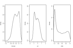
(a) data with $30$ subjects simulated from $y_{i}\sim SN(0.5g_{i}+0.5x_{i},0.25,0.5)$

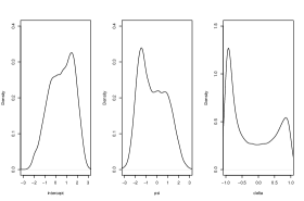
(b) data with $30$ subjects simulated from $y_{i}\sim SN(0.5g_{i}+0.5x_{i},1,0.5)$

Figure 1: Posterior densities of the intercept, $\psi$ and $\delta=\frac{\lambda}{\sqrt{1+\lambda^{2}}}$ in the univariate SN regression

6.1 Multimodality in the SN regression

In the univariate SN regression, the expected Fisher information matrix is singularAZZALINI:1985 at $\lambda=\psi/\sigma=0$. As a consequence, the empirical distribution of the MLE, and the posterior distribution of the parameter in Bayesian inference are often bimodal pewsey:2000 ; Arellano:2008 when $\lambda$ is near $0$. Liseo and Parisi liseo:2013 raises a concern that the Gibbs sampler chain can easily get stuck in one of the modes for multimodal posterior distributions.

This does not appear to be a concern in our algorithm possibly because we sample $(\bm{\theta}_{j},\gamma_{j})$’s simultaneously using the blocking scheme. The Gibbs sampler can be highly inefficient if the intercept and $\underline{\psi}_{j}$ are sampled separately because they are highly correlated. For illustrative purposes, we generate two datasets of size $n=30$ from $y_{i}\sim SN(\alpha_{1}+\alpha_{2}x_{i}+\alpha_{3}g_{i},\sigma^{2},\psi)$. Figure 1 plots the posterior densities of $\alpha_{1}$, $\psi$ and $\delta=\frac{\lambda}{\sqrt{1+\lambda^{2}}}$. They are clearly bimodal or multimodal for both datasets.

6.2 Analysis of an antidepressant trial using controlled imputation

The antidepressant trial has been analyzed by several authors to illustrate the missing data methodologies 2013:mallinckrodta ; 2015a:tang ; 2017:tanga ; 2017:tangb ; tang:2019 ; 2017:tangc . The Hamilton 17-item rating scale for depression ($\text{HAMD}_{17}$) is collected at baseline and weeks 1, 2, 4, 6. The dataset consists of 84 subjects on the experimental treatment and 88 subjects on placebo. The number of subjects who discontinue the trial early is $20$ ($24\%$) in the experimental arm, and $23$ ($26\%$) in the placebo arm.

The purpose of the analysis is to estimate the effect of the experimental product compared to placebo on the improvement in $\text{HAMD}_{17}$ from baseline to week $6$. We impute the missing response under MAR and MNAR by MMRM-n, MMRM-t, MMRM-sn and MMRM-st. The covariate set $\mathcal{X}$ includes the intercept, baseline $\text{HAMD}_{17}$ score $y_{i0}$ and treatment status $g_{i}$. The covariate set $\mathcal{Z}$ is empty. In each model, $m=10,000$ datasets are imputed from every $100$th iteration after a burn-in period of $100,000$ iterations. The trace plots and autocorrelation function (ACF) plots indicate approximate convergence of these MDA algorithms. In practice, it is prudent to use a long burn-in period to ensure that the Markov chain reaches the stationary distribution, and this is particularly important in the pharmaceutical industry where the analysis is done by programmers without much knowledge about the Bayesian analysis 2017:tanga . We analyze the outcome at week $6$ by the analysis of covariance (ANCOVA) for each imputed dataset, and the results are combined for inference using Rubin’s rule barnard:1999 .

We employ the deviance information criterion (DIC spiegelhalter:2002 ) to compare the four MMRMs. The DIC is defined as

$$\begin{aligned} \text{DIC}&=D(\hat{\bm{\eta}},\hat{\bm{\phi}},\hat{\nu})+2\text{pD}=D(\hat{\bm{\eta}},\hat{\bm{\phi}},\hat{\nu})+2[\bar{D}(\bm{\eta},\bm{\phi},\nu)-D(\hat{\bm{\eta}},\hat{\bm{\phi}},\hat{\nu})]\\ &=2m^{-1}\sum_{b=1}^{m}D(\bm{\eta}^{(b)},\bm{\phi}^{(b)},\nu^{(b)})-D(\hat{\bm{\eta}},\hat{\bm{\phi}},\hat{\nu}),\end{aligned}$$

where $D(\bm{\eta},\bm{\phi},\nu)=-2\sum_{i=1}^{n}\log[f(\bm{y}_{io}|\bm{\eta},\bm{\phi},\nu)]$, $(\bm{\eta}^{(b)},\bm{\phi}^{(b)},\nu^{(b)})$ is the $b$-th posterior sample collected after the burn-in period, $(\hat{\bm{\eta}},\hat{\bm{\phi}},\hat{\nu})=m^{-1}\sum_{b=1}^{m}(\bm{\eta}^{(b)},\bm{\phi}^{(b)},\nu^{(b)})$, and $\bar{D}(\bm{\eta},\bm{\phi},\nu)=m^{-1}\sum_{b=1}^{m}D\left(\bm{\eta}^{(b)},\bm{\phi}^{(b)},\nu^{(b)}\right)$. In DIC, $D(\hat{\bm{\eta}},\hat{\bm{\phi}},\hat{\nu})$ measures the model fit while pD estimates the effective number of parameters or model complexity spiegelhalter:2002 . Overall, a smaller DIC indicates a better model fit.

	MMRM-n		MMRM-t		MMRM-sn		MMRM-st
	mean$\pm$ SE	t (pvalue)	mean$\pm$ SE	t (pvalue)	mean$\pm$ SE	t (pvalue)	mean$\pm$ SE	t (pvalue)
MAR	$-2.80\pm 1.11$	$-2.54\,(0.012)$	$-2.81\pm 1.13$	$-2.49\,(0.014)$	$-2.80\pm 1.14$	$-2.47\,(0.015)$	$-2.81\pm 1.11$	$-2.54\,(0.012)$
J2R	$-2.13\pm 1.12$	$-1.90\,(0.059)$	$-2.11\pm 1.14$	$-1.85\,(0.066)$	$-2.14\pm 1.15$	$-1.87\,(0.064)$	$-2.16\pm 1.12$	$-1.93\,(0.056)$
CR	$-2.37\pm 1.10$	$-2.15\,(0.033)$	$-2.37\pm 1.11$	$-2.13\,(0.035)$	$-2.37\pm 1.12$	$-2.11\,(0.036)$	$-2.38\pm 1.10$	$-2.16\,(0.032)$
CIR	$-2.45\pm 1.10$	$-2.23\,(0.027)$	$-2.46\pm 1.12$	$-2.20\,(0.030)$	$-2.45\pm 1.13$	$-2.17\,(0.032)$	$-2.47\pm 1.10$	$-2.25\,(0.026)$
DEL(a)	$-2.05\pm 1.13$	$-1.82\,(0.071)$	$-2.05\pm 1.15$	$-1.78\,(0.076)$	$-2.06\pm 1.16$	$-1.78\,(0.078)$	$-2.07\pm 1.13$	$-1.83\,(0.069)$

Table 1: MI treatment effect estimates at week $6$ in sensitivity analysis of an antidepressant trial using controlled pattern imputations:
^(a) a delta adjustment of $-2$ is applied to subjects in the experimental arm after treatment discontinuation. MAR is assumed in the placebo arm.

Table 1 reports the MI results. The DIC is $3526.97$ for MMRM-n, $3528.58$ for MMRM-t, $3514.55$ for MMRM-sn and $3514.43$ for MMRM-st. MMRM-st appears to fit the data slightly better and give slightly more significant treatment effect estimates than MMRM-n, MMRM-t and MMRM-sn.

(a) pvalue$<0.05$ above the dashed horizontal line

(b) The symbols indicate the range of pvalue: ‘v’ pvalue$<0.0001$, ‘x’ pvalue$<0.001$, ‘o’ pvalue $<0.01$, ‘*’ pvalue$<0.05$

Figure 2: Plot of -$\log_{10}(\text{pvalue})$ in the tipping point analysis of an antidepressant trial with delta adjustment in the experimental arm (left) and in both treatment groups (right)

As will be discussed in the last section, we suggest conducting the missing value imputation based directly on MMRM-st without a model selection in large trials. Below we illustrate the tipping point analysis on basis of MMRM-st. Figure 2(a) plots the result when the adjustment is applied only in the experimental arm (i.e. MAR in the placebo arm). The treatment comparison becomes insignificant (pvalue$>0.05$) if the mean response among dropouts from the experimental arm is at least $1.4$ point worse at each visit compared to subjects who remain on the experimental treatment. Figure 2(b) plots the analysis with the delta adjustment in both arms. The treatment effect becomes insignificant only in a small region where $\Delta_{0}-\Delta_{1}\geq 1.4$ roughly holds.

6.3 Framingham cholesterol data

We analyze the Framingham cholesterol data to assess the robustness of MMRM-n, MMRM-t, MMRM-sn and MMRM-st in the presence of outliers. The data were first explored by Zhang and Davidian zhang:2001 to characterize changes in the cholesterol level over time, and assess the effect of age and gender. Two hundred subjects are randomly selected from the Framingham study. The cholesterol levels are measured at the beginning of the study and then every $2$ years for $10$ years.

In the literaturezhang:2001 ; ghidey:2004 ; jara:2008 ; lachos:2009 ; cabral:2012 , this dataset was typically fitted by a linear growth (LG) model with baseline age and gender as fixed effects and subject-specific random intercept and slopes, where the random effects and/or random errors are modeled by non-normal distributions. We provide an alternative approach to analyze the data

$$y_{ij}=\eta_{1}+\eta_{2}\,t_{ij}+\eta_{3}\,\text{sex}_{i}+\eta_{4}\,\text{age}_{i}+\xi_{ij},$$

where $y_{ij}$ is the cholesterol level divided by $100$ at visit $j$ for subject $i$, and $t_{ij}$ is $(\text{time}-5)/10$ with time measured in years from baseline. To compare the fixed effect estimates with those reported in the literature, we put $4$ covariates $\{1,t_{ij},\text{sex}_{i},\text{age}_{i}\}$ in the set $\mathcal{Z}$, and no covariate in $\mathcal{X}$. Another approach is to set $\mathcal{X}=\{1,\text{sex}_{i},\text{age}_{i}\}$ and $\mathcal{Z}=\{t_{ij}\}$, and it makes fewer assumptions on the relationship of age and gender with the cholesterol level. The within subject dependence is modeled by the multivariate normal, t, SN or ST distributions. Our model is more general than the LG model in that we don’t assume a structured covariance matrix.

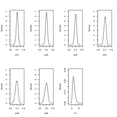
Figure 3: Marginal posterior densities for the skewness ($\psi_{1},\ldots,\psi_{6}$) and df ($\nu$) parameters in the analysis of the cholesterol raw data using MMRM-st

In the MDA algorithm, we collect $20,000$ posterior samples from every $100$th iteration after a burn-in period of $100,000$ iterations. The convergence of the Markov chain is evidenced by the trace plots and ACF plots in all four models.

Table 2 displays the parameter estimates and DIC. According to the DIC criterion, MMRM-st provides the best fit to the raw data. Figure 3 plots the marginal posterior densities for the skewness and df parameters in MMRM-st. The posterior samples of $\nu$ concentrate in the interval $[5,15]$, indicating heavy tails in the observed data. The posterior densities for $\psi_{1},\ldots,\psi_{6}$ all concentrate in the interval $[0.1,0.7]$, indicating the skewness in the cholesterol level at each visit. As shown in Table 2, the $95\%$ credible intervals for $\underline{\psi}_{3},\ldots,\underline{\psi}_{6}$ cover $0$, evidencing that the skewness of the cholesterol level reduces after adjusting for the historical outcomes at previous visits.

In these MMRMs, the regression coefficients (particularly the intercept $\eta_{1}$) do not have the same interpretation because the latent variable $\text{\small$\mathcal{W}$}\sim N^{+}(0,1)$ does not have zero mean. Let $E_{i}=\eta_{1}+\eta_{2}\,t_{ij}+\eta_{3}\,\text{sex}_{i}+\eta_{4}\,\text{age}_{i}$. In both MMRM-n and MMRM-t, the mean response is assumed to be constant over time, $\bm{E}_{i_{\text{n}}}=\bm{E}_{i_{\text{t}}}=(E_{i},E_{i},E_{i},E_{i},E_{i},E_{i})^{\prime}$. In MMRM-sn and MMRM-st, the mean response is not constrained to be the same across visits. The mean response profile is given by $\bm{E}_{i_{\text{sn}}}=\bm{E}_{i_{\text{n}}}+\sqrt{\frac{2}{\pi}}(\psi_{1},\ldots,\psi_{6})^{\prime}$ in MMRM-sn, and $\bm{E}_{i_{\text{st}}}=\bm{E}_{i_{\text{n}}}+\sqrt{\frac{\nu}{\pi}}\frac{\Gamma(\frac{\nu-1}{2})}{\Gamma(\frac{\nu}{2})}(\psi_{1},\ldots,\psi_{6})^{\prime}$ in MMRM-st. The Bayes estimates of the fixed effects in MMRM-n and MMRM-t are close to the MLE from the normal LG model reported by Zhang and Davidian zhang:2001 , and MMRM-t gives slightly narrower credible intervals for the fixed effects than MMRM-n. Lachos et al lachos:2009 analyzes the data using the robust LG model with SN (or ST) random intercept and slope, and normal (or t) random error, which can be roughly viewed as the submodels of the robust MMRM (15) with certain constraints on the covariance parameters $\Sigma$ and the skewness parameters $\bm{\psi}=(\psi_{1},\ldots,\psi_{p})^{\prime}$. The estimated age and gender effects [$\hat{\eta}_{3}=-0.057$ (SD: $0.049$), $\hat{\eta}_{4}=0.014$ (SD: $0.003$)] from the LG model with SN random effects are close to that from MMSM-sn, while the LG model with ST random effects gives similar estimates of the age and gender effects [$\hat{\eta}_{3}=-0.062$ (SD: $0.045$), $\hat{\eta}_{4}=0.014$ (SD: $0.003$)] to MMRM-st. The estimate and interpretation of the intercept $\eta_{1}$ and slope $\eta_{2}$ parameters are different in these models since the skewed random variables do not have zero mean. Lachos et al lachos:2010a assesses the performance of the robust LG models in predicting future responses. The robust MMRMs show comparable prediction performance, and the results are not shown due to limited space.

We evaluate the robustness of these MMRMs through the influence of the outliers on the parameter estimates. For simplicity, the outlier values are generated by replacing $y_{ij}$ with $y_{ij}=y_{ij}+8$ for $j=1,\ldots,6$ in the first two subjects. The result is also displayed in Table 2. In MMRM-n, the estimates of the regression coefficients and their $95\%$ credible intervals for the between-subject covariates (i.e. intercept $\eta_{1}$, sex $\eta_{3}$, age $\eta_{4}$) change noticeably after the introduction of the outliers, but the estimate of the time effect $\eta_{2}$ is little changed. Similar behavior is observed in the maximum likelihood inference by Zhang and Davidian zhang:2001 . In MMRM-sn, the outliers influence the estimates of the skewness parameters $\hat{\underline{\psi}_{j}}$’s and the $95\%$ credit intervals for the regression coefficients. MMRM-t provides robust parameter estimates except that the estimated df parameter gets smaller, indicating heavier tails in the presence of outliers. In MMRM-st, the outliers affect the estimates of the df and skewness parameters, but the estimation of the covariate effects is much less sensitive to the outliers.

	MMRM-n	MMRM-t	MMRM-sn	MMRM-st
Framingham cholesterol raw data
$\eta_{1}$	$1.647\pm 0.148\,\,[1.357,1.937]$	$1.567\pm 0.141\,\,[1.295,1.846]$	$1.395\pm 0.140\,\,[1.121,1.668]$	$1.414\pm 0.133\,\,[1.148,1.674]$
$\eta_{2}$	$0.275\pm 0.025\,\,[0.227,0.324]$	$0.277\pm 0.024\,\,[0.230,0.324]$	$0.332\pm 0.091\,\,[0.146,0.500]$	$0.296\pm 0.082\,\,[0.128,0.450]$
$\eta_{3}$	$-0.063\pm 0.054\,\,[-0.168,0.043]$	$-0.067\pm 0.051\,\,[-0.167,0.033]$	$-0.056\pm 0.049\,\,[-0.152,0.039]$	$-0.063\pm 0.046\,\,[-0.154,0.026]$
$\eta_{4}$	$0.017\pm 0.003\,\,[0.011,0.024]$	$0.018\pm 0.003\,\,[0.012,0.025]$	$0.014\pm 0.003\,\,[0.008,0.021]$	$0.014\pm 0.003\,\,[0.008,0.020]$
$\underline{\psi}_{1}$			$0.494\pm 0.065\,\,[0.358,0.609]$	$0.404\pm 0.061\,\,[0.277,0.517]$
$\underline{\psi}_{2}$			$0.334\pm 0.123\,\,[0.097,0.584]$	$0.271\pm 0.091\,\,[0.105,0.460]$
$\underline{\psi}_{3}$			$0.051\pm 0.120\,\,[-0.172,0.292]$	$0.073\pm 0.098\,\,[-0.115,0.269]$
$\underline{\psi}_{4}$			$0.116\pm 0.145\,\,[-0.148,0.407]$	$0.109\pm 0.105\,\,[-0.087,0.320]$
$\underline{\psi}_{5}$			$-0.225\pm 0.143\,\,[-0.478,0.083]$	$-0.136\pm 0.116\,\,[-0.353,0.097]$
$\underline{\psi}_{6}$			$-0.025\pm 0.168\,\,[-0.348,0.311]$	$0.023\pm 0.132\,\,[-0.234,0.288]$
$\nu$		$8.532\pm 2.058\,\,[5.472,13.458]$		$8.091\pm 1.869\,\,[5.275,12.542]$
DIC	$348.65$	$310.56$	$339.285$	$296.01$
Framingham cholesterol data with outliers generated in the first two subjects
$\eta_{1}$	$1.730\pm 0.356\,\,[1.034,2.425]$	$1.545\pm 0.147\,\,[1.258,1.834]$	$1.397\pm 0.190\,\,[1.011,1.756]$	$1.420\pm 0.139\,\,[1.144,1.689]$
$\eta_{2}$	$0.276\pm 0.024\,\,[0.229,0.324]$	$0.279\pm 0.024\,\,[0.234,0.326]$	$0.322\pm 0.032\,\,[0.260,0.385]$	$0.292\pm 0.056\,\,[0.181,0.399]$
$\eta_{3}$	$-0.019\pm 0.130\,\,[-0.273,0.236]$	$-0.067\pm 0.053\,\,[-0.171,0.037]$	$-0.050\pm 0.070\,\,[-0.189,0.089]$	$-0.065\pm 0.047\,\,[-0.157,0.028]$
$\eta_{4}$	$0.017\pm 0.008\,\,[0.001,0.033]$	$0.018\pm 0.004\,\,[0.012,0.025]$	$0.009\pm 0.004\,\,[0.000,0.017]$	$0.013\pm 0.003\,\,[0.006,0.019]$
$\underline{\psi}_{1}$			$1.159\pm 0.067\,\,[1.035,1.296]$	$0.468\pm 0.056\,\,[0.358,0.578]$
$\underline{\psi}_{2}$			$1.137\pm 0.249\,\,[0.592,1.613]$	$0.350\pm 0.101\,\,[0.167,0.563]$
$\underline{\psi}_{3}$			$0.197\pm 0.390\,\,[-0.522,1.031]$	$0.107\pm 0.113\,\,[-0.111,0.341]$
$\underline{\psi}_{4}$			$0.321\pm 0.461\,\,[-0.484,1.307]$	$0.138\pm 0.115\,\,[-0.074,0.379]$
$\underline{\psi}_{5}$			$-0.060\pm 0.447\,\,[-0.962,0.903]$	$-0.131\pm 0.128\,\,[-0.368,0.132]$
$\underline{\psi}_{6}$			$-0.059\pm 0.424\,\,[-0.966,0.801]$	$0.020\pm 0.131\,\,[-0.240,0.283]$
$\nu$		$4.957\pm 0.756\,\,[3.648,6.596]$		$5.318\pm 0.853\,\,[3.873,7.225]$
DIC	$699.60$	$402.50$	$544.95$	$371.94$

Table 2: DIC and posterior mean $\pm$ standard deviation [$95\%$ credible interval] for the model parameters in the analysis of the Framingham cholesterol raw data and data with outliers generated in the first two subjects :
[1] the estimates of the variance parameters (i.e. $\beta_{jk}$’s and $\gamma_{j}$’s) are omitted due to the limited space.

7 Discussion

We consider robust inference for skewed and/or heavy-tailed longitudinal data using MMRM-st, MMRM-sn or MMRM-t. These robust regressions have some undesirable attributes, and the posterior distributions can be improper with infinite estimates for some model parameters under diffuse priors. We use the PC prior for the df parameter, Huang-Wand’s huang:2013 hierarchical prior for $\Sigma$, and reference prior for the individual skewness parameter $\underline{\psi}_{j}$ of $\underline{y}_{ij}=y_{ij}-\sum_{t=1}^{j-1}\beta_{jt}y_{it}$. An efficient MDA algorithm is developed for Bayesian inference and missing data imputation. In practice, one may specify a different prior that reflects the existing knowledge or has better statistical properties. The MDA algorithm can be modified accordingly. For example, if a non-conjugate prior is used for the skewness parameters, they can be drawn via an independent or random walk Metropolis samplerchib:1995 with candidates generated by the proposed Gibbs scheme.

In clinical trials, usually only a few important covariates (e.g. baseline response, stratification factors) are included in the model chmp:2015 ; senn:1994 . These covariates are typically completely observed. In case there are some missing covariates, the MDA algorithm can be adapted to impute both the missing covariates and responses based on their joint distribution tang:2019 . In Lu lu:2010dd , the baseline covariates are constrained to have the same mean across treatment groups in randomized trials. Relaxing this constraint simplifies the algorithm without incurring efficiency loss in randomized trials (simulations unreported here), and makes it also suitable for studies with baseline imbalance.

The MDA algorithm is used to perform the controlled imputations for MNAR sensitivity analyses of longitudinal clinical trials. The assumptions about missing data are untestable given only the observed data NRC:2010 . A control-based strategy (CR, J2R or CIR) can be selected according to the drug mechanism of action (i.e. will the treatment benefit disappear after treatment discontinuation? how long will it take for the benefit to disappear?). The missing data mechanism may vary across patients, and one can apply the most conservative strategy (i.e. J2R) to patients who drop out due to lack of efficacy and safety issues. Alternatively, one may conduct the tipping point analysis based on the delta-adjusted imputation. There are many reasonable ways to assume how the response trajectory changes after treatment discontinuation. The MDA algorithm is still suitable as long as the observed data distribution remains the same as that under MAR.

In current clinical practice, it becomes more common to continue the data collection after treatment discontinuation. If the data observed after treatment discontinuation are assumed to have the same distribution as the missing data after dropout, they can be included in the controlled imputations by using the proposed MDA algorithm with little modifications. In the CR and delta-adjusted imputations, we replace the assigned treatment status by the actual treatment received at each visit (i.e. $0$ after treatment discontinuation) in models (11) and (16). In J2R and CIR, we need to use model (15), and code the actual treatment status by $p$ covariates in the covariate set $\mathcal{Z}$.

There are several reasons to implement the controlled imputations via MI. The analysis of clinical trials generally follows the intention-to-treat principle e9:1999 ; little:1996 , but the data are generated on an as-treated basis little:1996 . The MI inference can accommodate different imputation and analysis models. Furthermore, auxiliary variables and surrogate outcomes that are correlated with the response variables and the dropout process may be used to improve the imputation tang:2019 . Likelihood-based methods have been proposed for the control-based PMM lu:2014a . As demonstrated in the supplementary materials of Tang 2017:tangc , the likelihood-based approach is asymptotically equivalent to a MI approach in which both imputation and analysis models follow the as-treated principle, and hence may not be appropriate for the analysis of clinical trials. Furthermore, the standard maximum likelihood theory may not work in the SN and ST regressions since the asymptotic distribution for the MLE of the skewness parameters can be multimodal for data close to normal pewsey:2000 ; Arellano:2008 , and the MLE of the skewness parameters may be infinite for skewed data pewsey:2000 .

A variety of multivariate distributions have been proposed for skewed and heavy-tailed data. These include several versions of SN / ST distributions summarized by Lee and McLachlan lee:2013a , skew-slash distribution lachos:2009 , skew-contaminated normal distribution lachos:2009 , and finite mixtures of these distributions schnatter:2010 ; lee:2013a . One popular semiparametric approach is based on the Dirichlet process mixture model kleinman:1998 , which can be represented as an infinite mixture model. We choose the SN and ST distributions developed by Azzalini et al azzalini:1996 ; azzalini:2003 because they are easy to work with computationally and effective in handling non-normality for practical purposes. The MDA algorithm can be extended to MMRM with residual errors modeled by other non-normal distributions mentioned above. It is also possible to adapt the MDA algorithm as the monotone expectation-maximization algorithm for maximum likelihood inferences in these models.

We employ the MMRM model (10) or (15) for missing data imputation, which can be reorganized as a sequence of conditional models (11) or (16). We can also build the imputation process directly on models (11) or (16). As discussed in Tang tang:2019 , there are some advantages of using the sequential regression models. First, there is no need to include all the historical outcomes $(y_{i1},\ldots,y_{ij-1})$ as the predictors of $y_{ij}$ particularly when the number of response variables $p$ is large. Second, one can incorporate interactions between predictors into the conditional models.

In MMRM-st, the latent variables $(\text{\small$\mathcal{W}$}_{i},d_{i})$ are shared by all observations within a subject. It is more parsimonious than the sequential approach based on the univariate ST regression developed in our previous worktang:2019 , in which $p$ pairs of latent variables $(\text{\small$\mathcal{W}$}_{ij},d_{ij})$’s are introduced per subject. The sequential ST regression allows the skewness of $y_{ij}$’s to be induced by different latent variables, and the df to vary by visit / variable, and hence may be more suitable for multivariate data consisting of different outcomes (e.g. cholesterol, weight) than MMRM-st. Although the sequential ST regression seems more flexible, a large sample size is needed to accurately estimate VASCONCELLOS:2005 the df parameters and detect the difference in the df across visits since the likelihood function becomes flatter with increasing df. It may be preferable to use MMRM-st to analyze longitudinal data with the same response variable collected repeatedly over time if there is no big variation in the degrees of tail heaviness across visits.

Extensive research indicates that the analysis of non-normal outcomes based on the normality assumption may produce inefficient inferences possible because the violation of normality tends to have more impact on the estimation of the variance-covariance parameters and the variance of the fixed effects than on the estimation of the fixed effects pinheiro:2001 in both Bayesian inference lachos:2009 and maximum likelihood inference pinheiro:2001 ; zhang:2001 ; lange:1989 . This is also observed in the Bayesian analysis of the cholesterol data using MMRM-n. The Bayes parameter estimates in MMRM-st and MMRM-t are quite insensitive to the outliers.

As evidenced by the DIC criterion, MMRM-st provides the best fit to both the antidepressant trial and cholesterol data. In the MI inference, we recommend imputing missing values using MMRM-st, and there is no need to perform a model selection in large confirmatory trials. A model selection procedure may pick up a wrong model, inflating the type I error rate lukacs:2009 ; mundry:2009 . In our early work tang:2019 , simulation is conducted for the analysis of bivariate continuous and binary outcomes. It shows that the MI estimates from the ST regression have smaller bias and variance than that based on the normal regression for non-normal continuous outcomes, while the two approaches have almost the same efficiency for normal outcomes. There are numerical evidences that MMRM-st tends to outperform MMRM-n for non-normal longitudinal continuous outcomes. Inference based on a reduced model can be misleading if the corresponding assumption does not hold tang:2019 ; wang:2015 ; pinheiro:2001 . We will conduct a formal simulation study to compare these MMRMs after we find enough computational resources, and report the results elsewhere.

A future research direction associated with the robust MMRMs is to identify outliers or atypical observations wang:2015 ; pinheiro:2001 . This may help us better evaluate the treatment effects (e.g. is the effect of the test treatment driven by few subjects?). It is inappropriate to remove these atypical observations from the analysis as it affects the accuracy and precision of parameter estimates lange:1989 . In MI, we analyze the imputed data by ANCOVA, which may not be robust to a severe deviation from normality glass:1972 . The MI inference may be improved by analyzing the imputed data using a robust approach such as the M-estimation mehrotra:2012 .

ACKNOWLEDGEMENT

We would like to thank the associate editor and two referees for their helpful suggestions that improve the quality of the work.

Appendix A Appendix

A.1 Posterior distributions in the MDA algorithm

A.1.1 Posterior distribution of $(d_{i},\text{\small$\mathcal{W}$}_{i},$ $\bm{y}$${}_{im})$

Let $\tilde{\bm{y}}_{im}=(\text{\small$\mathcal{W}$}_{i},\bm{y}_{im})$ and $X_{i}=(x_{i1},\ldots,x_{iq},\bm{y}_{io}^{\prime})^{\prime}$. Let $U_{ij_{o}}$ and $U_{ij_{m}}$ be a partition of the $(\text{\small{$Q$}}+s_{i})\times 1$ vector $(\bm{\theta}_{j},-1,\bm{0}_{s_{i}-j}^{\prime})^{\prime}$ according to the elements in $X_{i}$ and $\tilde{\bm{y}}_{im}$. Let $y_{ij}^{*}=-U_{ij_{o}}^{\prime}X_{i}$ for model (10). For model (15), $y_{ij}^{*}=-U_{ij_{o}}^{\prime}X_{i}-\sum_{k=1}^{\text{\tiny{$R$}}}\eta_{k}\underline{z}_{ikj}$. The posterior distribution of $(d_{i},\text{\small$\mathcal{W}$}_{i},\bm{y}_{im})$ is given by

$$\begin{aligned} &\pi(d_{i},\text{\small$\mathcal{W}$}_{i},\bm{y}_{im}|\bm{y}_{io},\bm{\phi},\nu)\propto f(d_{i},\text{\small$\mathcal{W}$}_{i})\left[\prod_{j=1}^{s_{i}}\sqrt{d_{i}\gamma_{j}}\right]\exp\left[-\sum_{j=1}^{s_{i}}\frac{d_{i}\gamma_{j}(y_{ij}^{*}-U_{ij_{m}}^{{}^{\prime}}\tilde{\bm{y}}_{im})^{2}}{2}\right]\\ &\propto d_{i}^{\frac{\nu+s_{i}+1}{2}-1}\exp\left[-d_{i}\frac{b_{d}+(\tilde{\bm{y}}_{im}-\mu_{w_{i}})^{\prime}A_{w_{i}}(\tilde{\bm{y}}_{im}-\mu_{w_{i}})}{2}\right]\\ &\propto\left[1+\frac{\frac{(\text{\small$\mathcal{W}$}_{i}-\mu_{wi1})^{2}}{U_{w11}^{2}b_{d}/b_{a}}}{b_{a}}\right]^{-\frac{b_{a}+1}{2}}\mathcal{G}\left(d_{i}|\frac{b_{a}+1}{2},\frac{b_{d}+(\text{\small$\mathcal{W}$}_{i}-\mu_{wi1})^{2}L_{w11}^{2}}{2}\right)\\ &\qquad\qquad\qquad N\left(\bm{y}_{im}|\mu_{im},\frac{U_{w22}U_{w22}^{\prime}}{d_{i}}\right)\end{aligned}$$ (19)

subject to $\text{\small$\mathcal{W}$}_{i}>0$, where $\tilde{m}=m_{i}+1$, $A_{0}$ is a $\tilde{m}_{i}\times\tilde{m}_{i}$ matrix with $1$ at its $(1,1)$ entry and $0$ elsehwere, $A_{w_{i}}=A_{0}+\sum_{j=1}^{s_{i}}\gamma_{j}U_{ij_{m}}^{\prime}U_{ij_{m}}$, the lower triangle matrix $L_{w_{i}}=\begin{bmatrix}L_{w11}&\bm{0}\\ L_{w21}&L_{w22}\\ \end{bmatrix}$ satisfies $A_{w_{i}}=L_{w_{i}}^{\prime}L_{w_{i}}$, $L_{w11}$ is a scalar, $U_{w_{i}}=\begin{bmatrix}U_{w11}&\bm{0}\\ U_{w21}&U_{w22}\\ \end{bmatrix}=L_{w_{i}}^{-1}$, $B_{w_{i}}=\sum_{j=1}^{s_{i}}\gamma_{j}U_{ij_{m}}^{\prime}y_{ij}^{*}$, $C_{w_{i}}=U_{w_{i}}^{\prime}B_{w_{i}}$, and $\mu_{w_{i}}=A_{w_{i}}^{-1}B_{w_{i}}=U_{w_{i}}C_{w_{i}}=\begin{bmatrix}\mu_{wi1}\\ \mu_{wi2}\\ \end{bmatrix}$, $\mu_{im}=\mu_{wi2}+U_{w21}L_{w11}(\text{\small$\mathcal{W}$}_{i}-\mu_{wi1})$, $b_{a}=\nu+o_{i}$, $B_{w_{i}}^{\prime}A_{w_{i}}^{-1}B_{w_{i}}=C_{w_{i}}^{\prime}C_{w_{i}}$ and $b_{d}=\nu+\sum_{j=1}^{s_{i}}\gamma_{j}y_{ij}^{*2}-C_{w_{i}}^{\prime}C_{w_{i}}$. In SAS IML, $L_{w_{i}}$ can be computed can use the following syntax

        index=mtilde:1;
        Lwi = (root(Awi[index,index]))[index,index];

Equation (19) implies that we can draw $(\text{\small$\mathcal{W}$}_{i},d_{i},\bm{y}_{im})$ sequentially from

$$\begin{aligned} d_{i}^{*}&\sim\mathcal{G}\left(\frac{b_{a}}{2},\frac{b_{d}}{2}\right),\quad\text{\small$\mathcal{W}$}_{i}|d_{i}^{*}\sim N^{+}\left(\mu_{wi1},\frac{U_{w11}^{2}}{d_{i}}\right),\\ &\qquad\qquad d_{i}|\text{\small$\mathcal{W}$}_{i},d_{i}^{*}\sim\mathcal{G}\left(\frac{b_{a}+1}{2},\frac{b_{d}+(\text{\small$\mathcal{W}$}_{i}-\mu_{wi1})^{2}L_{w11}^{2}}{2}\right),\\ &\quad\,\bm{y}_{im}|d_{i},\text{\small$\mathcal{W}$}_{i},d_{i}^{*}\sim N\left(\mu_{im},\frac{U_{w22}U_{w22}^{\prime}}{d_{i}}\right).\end{aligned}$$ (20)

The marginal distribution of $\text{\small$\mathcal{W}$}_{i}$ is $t^{+}\left(\mu_{wi1},U_{w11}^{2}\frac{b_{d}}{b_{a}},b_{a}\right)$, but the marginal distribution of $d_{i}$ is not gamma due to the restriction $\text{\small$\mathcal{W}$}_{i}>0$.

The posterior distribution of $\bm{y}_{im}$ can be equivalently written as

$$\bm{y}_{im}|d_{i},\text{\small$\mathcal{W}$}_{i},\bm{y}_{io},\bm{\phi},\nu\sim N\left(\mu_{im},\frac{V_{y_{\text{m}}}}{d_{i}}\right),$$ (21)

where $h$ is the index of the first missing observation for subject $i$ in pattern $s$, $\tilde{U}_{ij_{m}}$ is a sub-vector of $(\bm{\theta}_{j},-1,\bm{0}_{s_{i}-j}^{\prime})^{\prime}$ corresponding to the elements in $\bm{y}_{im}$, $y_{ij}^{**}=y_{ij}^{*}-\psi_{j}\text{\small$\mathcal{W}$}_{i}$, $V_{y_{\text{m}}}=(\sum_{j=h}^{s}\gamma_{j}\tilde{U}_{ij_{m}}\tilde{U}_{ij_{m}}^{\prime})^{-1}$ and $\mu_{im}=\hat{V}_{y_{\text{m}}}\sum_{j=h}^{s}\gamma_{j}\tilde{U}_{ij_{m}}y_{ij}^{**}$.

A.1.2 Posterior distribution of $g$ in step PX1

The posterior distribution of $g$ with a Harr prior $g^{-1}$ and Jacobian $g^{n-p}$ is

$$\begin{aligned} \text{pos}(g)&\propto g^{n-p}g^{-1}\,\pi\left(Y_{m},gd_{1},\ldots,gd_{n},W,\bm{\theta}_{1},\frac{\gamma_{1}}{g},d_{1_{\text{\tiny$\psi$}}},\ldots,\bm{\theta}_{p},\frac{\gamma_{p}}{g},d_{p_{\text{\tiny$\psi$}}},\nu|Y_{o}\right)\\ &\propto g^{n-p}g^{-1}\prod_{i=1}^{n}\left\{\left(gd_{i}\right)^{\frac{\nu+1}{2}-1}\exp\left[-g\frac{d_{i}(\nu+\text{\small$\mathcal{W}$}_{i}^{2})}{2}\right]\right\}\\ &\,\,\,\,\,\,\,\,\,\,\,\prod_{j=1}^{p}\left\{\left(\frac{\gamma_{j}}{g}\right)^{\frac{n_{w}+2j+r-p-3}{2}}\exp\left[-\frac{\gamma_{j}\tilde{\bm{\theta}}_{j}^{\prime}E_{j}\tilde{\bm{\theta}}_{j}}{2g}\right]\right\}\\ &\propto g^{\frac{n(1+\nu)-p(n_{w}+r)}{2}-1}\exp\left[-g\frac{\sum_{i=1}^{n}d_{i}(\nu+\text{\small$\mathcal{W}$}_{i}^{2})}{2}\right]\exp\left[-\frac{\sum_{j=1}^{p}\gamma_{j}\tilde{\bm{\theta}}_{j}^{\prime}E_{j}\tilde{\bm{\theta}}_{j}}{2g}\right].\end{aligned}$$

A.1.3 Posterior distribution of $h$ in step PX2

The posterior distribution of $h$ with a Harr prior $h^{-1}$ and Jacobian $h^{n-p}$ is

$$\begin{aligned} \text{pos}(h)\propto h^{n-p}h^{-1}\exp\left(-h^{2}\frac{\sum_{i=1}^{n}d_{i}\text{\small$\mathcal{W}$}_{i}^{2}}{2}\right)\exp\left(-\frac{\sum_{j=1}^{p}\gamma_{j}\underline{\psi}_{j}^{2}\frac{4d_{j_{\text{\tiny$\psi$}}}}{\pi^{2}}}{2h^{2}}\right).\end{aligned}$$

The posterior distribution of $H=h^{2}$ is

$$\text{pos}(H)\propto\text{pos}(h)\left|\frac{\partial h}{\partial H}\right|\propto H^{\frac{n-p}{2}-1}\exp\left(-H\frac{\sum_{i=1}^{n}d_{i}\text{\small$\mathcal{W}$}_{i}^{2}}{2}\right)\exp\left(-\frac{\sum_{j=1}^{p}\gamma_{j}\underline{\psi}_{j}^{2}\frac{4d_{j_{\text{\tiny$\psi$}}}}{\pi^{2}}}{2H}\right).$$

A.1.4 Prior and posterior distributions of $\nu$

We firstly derive the PC prior for $\nu$. The Kullback-Leibler (KL) distance between the multivariate t distribution $t(\bm{\mu},\frac{\nu-2}{\nu}\Sigma,\nu)$ and the normal distribution $N(\bm{\mu},\Sigma)$ is

$$\begin{aligned} \text{KL}(\nu)&=\int t\left(\bm{x}|\bm{\mu},\frac{\nu-2}{\nu}\Sigma,\nu\right)\log t\left(\bm{x}|\bm{\mu},\frac{\nu-2}{\nu}\Sigma,\nu\right)d\bm{x}\\ &\,\,\,\,\,\,\,\,\,\,\,\,\,\,\,\,-\int t\left(\bm{x}|\bm{\mu},\frac{\nu-2}{\nu}\Sigma,\nu\right)\log\phi(\bm{x}|\bm{\mu},\Sigma)d\bm{x}\\ &=\frac{p}{2}\left[1+\log\left(\frac{2}{\nu-2}\right)\right]+\log\Gamma\left(\frac{\nu+p}{2}\right)-\log\Gamma\left(\frac{\nu}{2}\right)\\ &\,\,\,\,\,\,\,\,\,\,\,\,\,\,\,\,-\frac{\nu+p}{2}\left[\Psi\left(\frac{\nu+p}{2}\right)-\Psi\left(\frac{\nu}{2}\right)\right].\end{aligned}$$

since the first integration equals $\log\Gamma\left(\frac{\nu+p}{2}\right)-\log\Gamma\left(\frac{\nu}{2}\right)-\frac{\nu+p}{2}\left[\Psi\left(\frac{\nu+p}{2}\right)-\Psi\left(\frac{\nu}{2}\right)\right]-\frac{1}{2}\log|\Sigma|-\frac{p}{2}\log(\nu-2)-\frac{p}{2}\log(\pi)$ by Kotz and Nadarajah kotz:2004 , and the second integration equals $-\frac{p}{2}\log(2\pi)-\frac{1}{2}\log|\Sigma|-\frac{p}{2}$.

By the definition of the PC prior simpson:2017 , the density is $\lambda\exp(-\lambda d(\nu))\left|\frac{\partial d(\nu)}{\partial{\nu}}\right|$, where $d(\nu)=\sqrt{2\text{KL}(\nu)}$.

The posterior distribution of $\nu$ is given by

$$\begin{aligned} &\pi(\nu|\Sigma,\bm{\psi},\theta_{j},\gamma_{j})\propto\pi(\nu)\prod_{i=1}^{n}t_{p}(\bm{y}_{io}|\bm{\mu}_{io},\Omega_{io},\nu)\\ &\,\,\,\,\,\,\,\,\,\,\,\,\,\,\,\,\,\,\,\,T_{\nu+o_{i}}\left[\bm{\lambda}_{io}^{*^{\prime}}(\bm{y}_{io}-\bm{\mu}_{io})\sqrt{\frac{\nu+o_{i}}{\nu+(\bm{y}_{io}-\bm{\mu}_{io})^{\prime}\Omega_{io}^{-1}(\bm{y}_{io}-\bm{\mu}_{io})}}\,\right]I(\nu>\nu_{l}),\end{aligned}$$

where $t_{p}(\bm{y}_{io}|\bm{\mu}_{io},\Omega_{io},\nu)\propto\frac{\Gamma(\frac{\nu+o_{i}}{2})}{\Gamma(\frac{\nu}{2})\nu^{o_{i}/2}}[1+(\bm{y}_{io}-\bm{\mu}_{io})^{\prime}\Omega_{io}^{-1}(\bm{y}_{io}-\bm{\mu}_{io})/\nu]^{-\frac{\nu+o_{i}}{2}}$, and $\bm{\lambda}_{io}^{*}=\Sigma_{io}^{-1}\bm{\psi}_{io}/\sqrt{1+\bm{\psi}_{io}^{\prime}\Sigma_{io}^{-1}\bm{\psi}_{io}}$.

For subjects with no intermittent missing data, the skew-t density function can be computed without matrix inversion using the following relationship $\bm{\lambda}_{io}^{*^{\prime}}(\bm{y}_{io}-\bm{\mu}_{io})=\sum_{t=1}^{s}\lambda_{t}R_{t}\underline{\psi}_{t}$ and $(\bm{y}_{io}-\bm{\mu}_{io})^{\prime}\Omega_{io}^{-1}(\bm{y}_{io}-\mu_{io})=\sum_{t=1}^{s}\lambda_{t}r_{t}^{2}-[\sum_{t=1}^{s}\lambda_{t}r_{t}\underline{\psi}_{t}]^{2}/[1+\sum_{t=1}^{s}\lambda_{t}\underline{\psi}_{t}^{2}]$, where $r_{j}=y_{ij}-\sum_{t=1}^{j-1}\beta_{jt}y_{it}-\sum_{k=1}^{\text{\tiny{$Q$}}}\underline{\alpha}_{kj}x_{ik}$ for model (10) and $r_{j}=y_{ij}-\sum_{t=1}^{j-1}\beta_{jt}y_{it}-\sum_{k=1}^{\text{\tiny{$R$}}}\eta_{k}\underline{z}_{ikj}-\sum_{k=1}^{\text{\tiny{$Q$}}}\underline{\alpha}_{kj}x_{ik}$ for model (15).

The candidate $\nu^{*}$ is generated from $\log(\nu^{*}-\nu_{l})\sim N[\log(\nu-\nu_{l}),c^{2}]$. It will be accepted with probability $\alpha_{\nu}=\min\left\{1,\frac{(\nu^{*}-\nu_{l})\pi(\nu^{*})\prod_{i=1}^{n}f(\bm{y}_{io}|\bm{\theta}_{i},\gamma_{i},\nu^{*})}{(\nu-\nu_{l})\pi(\nu)\prod_{i=1}^{n}f(\bm{y}_{io}|\bm{\theta}_{i},\gamma_{i},\nu)}\right\}$.

A.2 Adaption of the MDA algorithm for MMRM-sn

For MMRM-sn (i.e. $\nu\equiv\infty$), the MDA algorithm $A$ can easily adapted by ignoring steps P2 and PX1, and setting $d_{i}\equiv 1$ and $d_{i}^{*}\equiv 1$ in drawing $(\bm{\theta}_{j},\gamma_{j},d_{\psi_{j}},\rho_{j})$’s and $(\text{\small$\mathcal{W}$}_{i},\bm{y}_{im})$’s. For example, $(\text{\small$\mathcal{W}$}_{i},\bm{y}_{im})$ in step I can be imputed by modifying the posterior distribution (20) as

$$\text{\small$\mathcal{W}$}_{i}\sim N^{+}(\mu_{wi1},U_{w11}^{2})\,\text{ and }\,\bm{y}_{im}|\text{\small$\mathcal{W}$}_{i}\sim N(\mu_{im},U_{w22}U_{w22}^{\prime}).$$

A.3 Adaption of the MDA algorithm for MMRM-t

For MMRM-t (i.e. $\underline{\psi}_{j}\equiv 0$ for $j=1,\ldots,p$, $\text{\small$\mathcal{W}$}_{i}\equiv 0$), the MDA algorithm $A$ needs the following modifications:
1. Step PX2 is no longer needed.
2. Step P1: Remove $\text{\small$\mathcal{W}$}_{i}$ from the model. Set $d_{\psi_{j}}\equiv 0$ and $\bm{\theta}_{j}=(\underline{\alpha}_{1j},\ldots,\underline{\alpha}_{qj},\beta_{j1},\ldots,\beta_{jj-1})^{\prime}$. Sample $(\bm{\theta}_{j},\gamma_{j})$’s from

$$\begin{aligned} \pi(\bm{\theta}_{j},\gamma_{j}|d_{i}\text{'s},\nu,Y_{o},Y_{m})\propto\gamma_{j}^{\frac{n_{w}+2j+r^{*}-p-1}{2}-1}\exp\left[-\frac{\gamma_{j}}{2}\tilde{\bm{\theta}}_{j}^{\prime}(E_{j}+\sum_{i\leq n_{j}}d_{i}\tilde{\bm{x}}_{ij}\tilde{\bm{x}}_{ij}^{\prime})\tilde{\bm{\theta}}_{j}\right]\end{aligned}$$

for $j=1,\ldots,p$, where $E_{j}$ is the $(q+j)\times(q+j)$ leading principle submatrix of the $(q+p)\times(q+p)$ matrix $E=\begin{bmatrix}M&M\bm{\alpha}_{0}^{\prime}\\ \bm{\alpha}_{0}M&\bm{\alpha}_{0}M\bm{\alpha}_{0}^{\prime}+A_{w}\\ \end{bmatrix}$ and $r^{*}$ is the rank of $M$. If the inverse Wishart or Jeffrey’s prior (with fixed $A_{w}$ and $n_{w}$) instead of the hierarchical prior of Huang and Wand huang:2013 is used, step P0 shall be ignored.
3. Step I: draw $d_{i}\sim\mathcal{G}\left(\frac{b_{a}}{2},\frac{b_{d}}{2}\right)$ and $\bm{y}_{im}\sim N(\mu_{w_{i}},(d_{i}A_{w_{i}})^{-1})$ since

$$\begin{aligned} \pi(d_{i},&\bm{y}_{im}|\bm{y}_{io},\nu,\bm{\phi})\propto f(d_{i})d_{i}^{\frac{s_{i}}{2}}\exp\left[-\frac{\sum_{j=1}^{s_{i}}d_{i}\gamma_{j}(y_{ij}^{*}-\tilde{U}_{ij_{m}}^{\prime}\bm{y}_{im})^{2}}{2}\right]\\ \propto&\left\{d_{i}^{\frac{\nu+o_{i}}{2}-1}\exp\left[-\frac{d_{i}b_{d}}{2}\right]\right\}\left\{d_{i}^{\frac{m_{i}}{2}}\exp[-\frac{d_{i}(\bm{y}_{im}-\mu_{w_{i}})^{\prime}A_{w_{i}}(\bm{y}_{im}-\mu_{w_{i}})}{2}]\right\},\end{aligned}$$

where $f(d_{i})\propto d_{i}^{\nu/2-1}\exp(-d_{i}\nu)$, $A_{w_{i}}=\sum_{j=1}^{s_{i}}\gamma_{j}\tilde{U}_{ij_{m}}^{\prime}\tilde{U}_{ij_{m}}$, $B_{w_{i}}=\sum_{j=1}^{s_{i}}\gamma_{j}\tilde{U}_{ij_{m}}^{\prime}y_{ij}^{*}$, $\mu_{w_{i}}=A_{w_{i}}^{-1}B_{w_{i}}$, $b_{a}=\nu+o_{i}$ and $b_{d}=\nu+\sum_{j=1}^{s_{i}}\gamma_{j}y_{ij}^{*2}-B_{w_{i}}^{\prime}A_{w_{i}}^{-1}B_{w_{i}}$.
4. Step PX1: $g$ is randomly drawn from
$g^{\frac{n\nu-p(n_{w}+r^{*})}{2}-1}\exp\left[-g\frac{\nu\sum_{i=1}^{n}d_{i}}{2}\right]\exp\left[-\frac{\sum_{j=1}^{p}\gamma_{j}\tilde{\bm{\theta}}_{j}^{\prime}E_{j}\tilde{\bm{\theta}}_{j}}{2g}\right]$.

References

- (1) Siddiqui O, Hung JHM and O’Neill R. MMRM vs. LOCF: A comprehensive comparison based on simulation study and 25 NDA datasets. Journal of Biopharmaceutical Statistics 2009; 19: 227–46.
- (2) Mallinckrodt CH, Lane PW, Schnell D et al. Recommendations for the primary analysis of continuous endpoints in longitudinal clinical trials. Drug Information Journal 2008; 42: 303 – 19.
- (3) ICH E9. Statistical principles for clinical trials: ICH harmonized tripartite guideline. Statistics in Medicine 1999; 18: 1905 – 42.
- (4) CHMP. Guideline on adjustment for baseline covariates in clinical trials. London: CHAMP, 2015.
- (5) Laird NM, Lange N and Stram D. Maximum likelihood computations with repeated measures: Application of the EM algorithm. Journal of the American Statistical Association 1987; 82: 97 – 105.
- (6) Tang Y. Closed-form REML estimators and sample size determination for mixed effects models for repeated measures under monotone missingness. Statistics in Medicine 2017; 36: 2135 – 2147.
- (7) Lu K and Mehrotra DV. Specification of covariance structure in longitudinal data analysis for randomized clinical trials. Statistics in Medicine 2010; 29: 474 – 88.
- (8) Gurka MJ, Edwards LJ and Muller KE. Avoiding bias in mixed model inference for fixed effects. Statistics in Medicine 2011; 30: 2696 – 707.
- (9) Jacqmin-Gadda H, Sibillot S, Proust C et al. Robustness of the linear mixed model to misspecified error distribution. Computational Statistics & Data Analysis 2007; 51: 5142 – 54.
- (10) Gomez EV, Schaalje GB and Fellingham GW. Performance of the Kenward-Roger method when the covariance structure is selected using AIC and BIC. Communications in Statistics-Simulation and Computation 2005; 34: 377 – 92.
- (11) Little R and Yau L. Intent-to-treat analysis for longitudinal studies with drop-outs. Biometrics 1996; 52: 1324 – 33.
- (12) Carpenter J, Roger J and Kenward M. Analysis of longitudinal trials with protocol deviation: a framework for relevant, accessible assumptions, and inference via multiple imputation. Journal of Biopharmaceutical Statistics 2013; 23: 1352 – 71.
- (13) Mallinckrodt C, Roger J, Chuang-stein C et al. Missing data: Turning guidance into action. Statistics in Biopharmaceutical Research 2013; 5: 369 – 82.
- (14) Tang Y. An efficient multiple imputation algorithm for control-based and delta-adjusted pattern mixture models using SAS. Statistics in Biopharmaceutical Research 2017; 9: 116 – 25.
- (15) Rubin DB. Inference and missing data. Biometrika 1976; 63: 581–92.
- (16) ICH E9 (R1) addendum on estimands and sensitivity analysis in clinical trials to the guideline on statistical principles for clinical trials. http://www.ema.europa.eu/docs/en_GB/document_library/Scientific_guideline/2017/08/WC500233916.pdf, 2017.
- (17) CHMP. EMA Guideline on Missing data in Confirmatory Clinical Trials (EMA/CPMP/EWP/1776/99). London: CHAMP, 2010.
- (18) National Research Council. Panel on Handling Missing Data in Clinical Trials. Committee on National Statistics, Division of Behavioral and Social Sciences and Education. The prevention and treatment of missing data in clinical trials. The National Academies Press: Washington, DC, 2010.
- (19) Little RJA. Pattern-mixture models for multivariate incomplete data. Journal of the Amerian Statistical Association 1993; 88: 125 – 34.
- (20) Tang Y. An efficient monotone data augmentation algorithm for multiple imputation in a class of pattern mixture models. Journal of Biopharmaceutical Statistics 2017; 27: 620 – 38.
- (21) Schafer JL. Analysis of Incomplete Multivariate Data. Chapman Hall, London, 1997.
- (22) Tang Y. Controlled pattern imputation for sensitivity analysis of longitudinal binary and ordinal outcomes with nonignorable dropout. Statistics in Medicine 2018; 37: 1467 – 81.
- (23) Tang Y. A monotone data augmentation algorithm for multivariate nonnormal data: with applications to controlled imputations for longitudinal trials. Statistics in Medicine 2019; 38: 1715 – 33.
- (24) Azzalini A. A class of distributions which includes the normal ones. Scandinavian Journal of Statistics 1985; 12: 171 – 78.
- (25) Azzalini A and Capitanio A. Distributions generated by perturbation of symmetry with emphasis on a multivariate skew t distribution. Journal of the Royal Statistical Society, Series B 2003; 65: 367 – 389.
- (26) Verbeke G and Lesaffre E. The effect of misspecifying the random effects distribution in linear mixed models for longitudinal data. Computational Statistics & Data Analysis 1997; 23: 541 – 56.
- (27) Pinheiro JC, Liu CH and Wu YN. Efficient algorithms for robust estimation in linear mixed-effects models using a multivariate t-distribution. Journal of Computational and Graphics Statistics 2001; 10: 249–76.
- (28) Zhang D and Davidian M. Linear mixed models with flexible distributions of random effects for longitudinal data. Biometrics 2001; 57: 795 – 802.
- (29) Arnau J, Bendayan R, Blanca MJ et al. The effect of skewness and kurtosis on the robustness of linear mixed models. Behavior Research Methods 2013; 45: 873 – 79.
- (30) Boos DD and Hughes-Oliver JM. How large does n have to be for z and t intervals? The American Statistician 2000; 54: 121 – 28.
- (31) von Hippel PT. Should a normal imputation model be modified to impute skewed variables? Sociological Methods and Research 2013; 42: 105– 38.
- (32) Azzalini A and Dalla Valle A. The multivariate skew-normal distribution. Biometrika 1996; 83: 715–726.
- (33) Liu C. Missing data imputation using the multivariate t distribution. Journal of Multivariate Analysis 1995; 53: 139–58.
- (34) Jara A, Quintana F and Martin ES. Linear mixed models with skew-elliptical distributions: A Bayesian approach. Computational Statistics and Data Analysis 2008; 52: 5033 – 45.
- (35) Lachos VH, Dey DK and Cancho VG. Robust linear mixed models with skew-normal independent distributions from a Bayesian perspective. Journal of Statistical Planning and Inference 2009; 139: 4098 – 110.
- (36) Arnold BC and Beaver RJ. Skewed multivariate models related to hidden truncation and/or selective reporting. Test 2002; 11: 7–54.
- (37) Arellano-Valle RB RB, Branco MD and Genton MG. A unified view on skewed distributions arising from selections. The Canadian Journal of Statistics 2006; 34: 581–601.
- (38) Liseo B and Loperfido N. A note on reference priors for the scalar skew-normal distribution. Journal of Statistical Planning and Inference 2006; 136: 373 – 389.
- (39) Bayes CL and Branco MD. Bayesian inference for the skewness parameter of the scalar skew-normal distribution. Brazilian Journal of Probability and Statistics 2007; 21: 141 – 163.
- (40) Branco MD, MGG and Liseo B. Objective Bayesian analysis of skew-t distributions. Scandinavian Journal of Statistics 2013; 40: 63– 85.
- (41) Pewsey A. Problems of inference for Azzalini’s skew-normal distribution. Journal of applied Statistics 2000; 27: 859 – 870.
- (42) Arellano-Valle R and Azzalini A. The centred parametrization for the multivariate skew-normal distribution. Journal of Multivariate Analysis 2008; 99: 1362 – 82.
- (43) Liseo B and Parisi A. Bayesian inference for the multivariate skew-normal model: A population Monte Carlo approach. Computational Statistics and Data Analysis 2013; 63: 125 – 138.
- (44) Fonseca TCO, Ferreira MAR and Migon HS. Objective Bayesian analysis for the Student-t regression model. Biometrika 2008; 95: 325 – 333.
- (45) Liu JS and Wu YN. Parameter expansion for data augmentation. Journal of the American Statistical Association 1999; 94: 1264 – 74.
- (46) Liu JS and Sabatti C. Generalised Gibbs sampler and multigrid Monte Carlo for Bayesian computation. Biometrika 2000; 87: 353–69.
- (47) Lee SX and McLachlan GJ. On mixtures of skew normal and skew t-distributions. Advances in Data Analysis and Classification 2013; 7: 241 – 66.
- (48) Fruhwirth-Schnatter S and Pyne S. Bayesian inference for finite mixtures of univariate and multivariate skew-normal and skew-t distributions. Biostatistics 2010; 11: 317 – 336.
- (49) Huang A and Wand MP. Simple marginally noninformative prior distributions for covariance matrices. Bayesian Analysis 2013; 8: 439 – 452.
- (50) Gelman A. Prior distributions for variance parameters in hierarchical models. Bayesian Analysis 2006; 1: 515 – 534.
- (51) Tang Y. An efficient monotone data augmentation algorithm for Bayesian analysis of incomplete longitudinal data. Statistics & Probability Letters 2015; 104: 146 – 52.
- (52) Simpson D, Rue H, Riebler A et al. Penalising model component complexity: A principled, practical approach to constructing priors. Statistical Science 2017; 32: 1–28.
- (53) Daniels MJ and Kass RE. Nonconjugate bayesian estimation of covariance matrices and its use in hierarchical models. JASA 1999; 94: 1254 – 63.
- (54) Permutt T. Sensitivity analysis for missing data in regulatory submission. Statistics in Medicine 2016; 35: 876 – 9.
- (55) Lu K, Li D and Koch GG. Comparison between two controlled multiple imputation methods for sensitivity analyses of time-to-event data with possibly informative censoring. Statistics in Biopharmaceutical Research 2015; 7: 199–213.
- (56) Tang Y. On the multiple imputation variance estimator for control-based and delta-adjusted pattern mixture models. Biometrics 2017; 73: 1379 – 87.
- (57) Tang Y. Controlled pattern imputation for sensitivity analysis of longitudinal binary and ordinal outcomes with nonignorable dropout. Statistics in Medicine 2018; 37: 1467 – 81.
- (58) Tang Y. Algorithms for imputing partially observed recurrent events with applications to multiple imputation in pattern mixture models. Journal of Biopharmaceutical Statistics 2018; 28: 518–33.
- (59) Barnard J and Rubin DB. Small-sample degrees of freedom with multiple imputation. Biometrika 1999; 86: 948 – 55.
- (60) Spiegelhalter D, Best N, Carlin B et al. Bayesian measures of model complexity and fit. Journal of the Royal Statistical Society, Series B 2002; 64: 583 – 639.
- (61) Ghidey W, Lesaffre E and Eilers P. Smooth random effects distribution in a linear mixed model. Biometrics 2004; 60: 945 – 53.
- (62) Cabral CRB, Lachos VH and Madruga MR. Bayesian analysis of skew-normal independent linear mixed models with heterogeneity in the random-effects population. Journal of Statistical Planning and Inference 2012; 142: 181 – 200.
- (63) Lachos VH, Ghosh P and Arellano-Valle RB. Likelihood based inference for skew normal independent linear mixed models. Statistica Sinica 2010; 20: 303 – 22.
- (64) Chib S and Greenberg E. Understanding the metropolis-hastings algorithm. American Statistician 1995; 49: 327 – 35.
- (65) Senn S. Testing for baseline balance in clinical trials. Statistics in Medicine 1994; 13: 1715 – 26.
- (66) Lu K. On efficiency of constrained longitudinal data analysis versus longitudinal analysis of covariance. Biometrics 2010; 66: 891 – 96.
- (67) Lu K. An analytic method for the placebo-based pattern-mixture model. Statistics in Medicine 2014; 33: 1134–45.
- (68) Kleinman KP and Ibrahim JG. A semiparametric bayesian approach to the random effects model. Biometrics 1998; 54: 921 – 38.
- (69) Vasconcellos KLP and Da Silva SG. Corrected estimates for student t regression models with unknown degrees of freedom. Journal of Statistical Computation and Simulation 2005; 52: 409 – 23.
- (70) Lange KL, Little RJA and Taylor JMG. Robust statistical modeling using the t-distribution. Journal of the American Statistical Association 1989; 84: 881 – 96.
- (71) Lukacs PM, Burnham KP and Anderson DR. Model selection bias and Freedman’s paradox. Ann Inst Stat Math 2009; 62: 117 – 25.
- (72) Mundry R and Nunn CL. Stepwise model fitting and statistical inference: turning noise into signal pollution. American Naturalist 2009; 173: 119 – 23.
- (73) Wang J and Luo S. Bayesian multivariate augmented beta rectangular regression models for patient-reported outcomes and survival data. Statistical Methods in Medical Research 2017; 26: 117 – 25.
- (74) Glass GV, Peckham PD and Sanders JR. Consequences of failure to meet assumptions underlying the fixed effects analyses of variance and covariance. Review of Educational Research 1972; 42: 237 – 88.
- (75) Mehrotra DV, Li X, Liu J et al. Analysis of longitudinal clinical trials with missing data using multiple imputation in conjunction with robust regression. Biometrics 2012; 68: 1250 – 9.
- (76) Kotz S and Nadarajah S. Multivariate t-distributions and their applications. Cambridge University Press, 2004.