Cooper pairing of incoherent electrons: an electron-phonon version of the Sachdev-Ye-Kitaev model

Abstract

We introduce and solve a model of interacting electrons and phonons that is a natural generalization of the Sachdev-Ye-Kitaev-model and that becomes superconducting at low temperatures. In the normal state two Non-Fermi liquid fixed points with distinct universal exponents emerge. At weak coupling superconductivity prevents the onset of low-temperature quantum criticality, reminiscent of the behavior in several heavy-electron and iron-based materials. At strong coupling, pairing of highly incoherent fermions sets in deep in the Non-Fermi liquid regime, a behavior qualitatively similar to that in underdoped cuprate superconductors. The pairing of incoherent time-reversal partners is protected by a mechanism similar to Anderson’s theorem for disordered superconductors. The superconducting ground state is characterized by coherent quasiparticle excitations and higher-order bound states thereof, revealing that it is no longer an ideal gas of Cooper pairs, but a strongly coupled pair fluid. The normal-state incoherency primarily acts to suppress the weight of the superconducting coherence peak and reduce the condensation energy. Based on this we expect strong superconducting fluctuations, in particular at strong coupling.

I Introduction

Superconductivity is the ultimate fate of a Fermi liquid at low temperaturesCooper1956 ; Bardeen1957lett ; Bardeen1957 ; Kohn1965 . A key assumption that gives rise to this Cooper instability is that the excitations of a Fermi liquid are slowly-decaying Landau quasiparticles with the same quantum numbers as free fermions. The resulting superconducting ground state can be understood as an ideal gas of Cooper pairs. Since superconductivity occurs in many systems where such sharp excitations are absent, the conditions for pairing of incoherent electrons is an important open problem. The emergence of a sharp superconducting coherence peak of small weight from a broad and structureless normal-state spectrum is in fact one of the hallmarks of the cuprate superconductorsDessau1991 ; ZXSchrieffer1997 ; Campuzano1996 ; Fedorov1999 ; Feng2000 , where the weight of the coherence peak was shown to be strongly correlated with the superfluid stiffness and the condensation energyFeng2000 . Key questions in this context are: Can one form Cooper pairs from completely incoherent fermions? Are there sharp quasi-particles in such a superconductor? Is the Cooper pair fluid that emerges still an ideal gas of pairs?

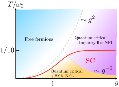
Figure 1: Schematic phase diagram of the SYK-model for electron-boson coupling as function of the dimensionless coupling constant $g=\bar{g}/\omega_{0}^{3/2}$, where $\omega_{0}$ is the bare phonon frequency. At lowest $T$ the normal state would be a Non-Fermi liquid state with anomalous exponents, similar to other SYK models. For $g<1$ superconductivity sets in at $T_{c}/\omega_{0}\propto g^{2}$, comparable to the temperature where quantum critical SYK-NFL sets in. Thus pairing occurs instead of the low-$T$ quantum critical state. At strong coupling a new intermediate-temperature regime opens up that is characterized by fully incoherent fermions. Coherent pairing of such incoherent fermions is still possible with finite transition temperature $T_{c}\rightarrow 0.112\omega_{0}$.

To address these questions in a theoretically well-controlled way it is highly desirable to identify a solvable model for non-quasiparticle superconductivity. A crucial issue is the proper interplay of Non-Fermi liquid excitations and the pairing interaction. For example, the spectral function of a Fermi liquid right at the Fermi surface,

$$A_{{\rm FL}}\left(\omega\right)=Z_{{\rm FL}}\delta\left(\omega\right),$$ (1)

is expected to transform for a quantum-critical system to the power-law form

$$A_{{\rm QC}}\left(\omega\right)=A_{0}\left|\omega\right|^{2\Delta-1}$$ (2)

with exponent $\Delta$. For $\Delta>0$ an evaluation of the pairing susceptibility with instantaneous pairing interaction yields no Cooper instabilityBalatsky1993 ; Sudbo1995 ; Yin1996 . Superconductivity would then only occur if the pairing interactions exceeded a threshold value. Then a superconducting ground state would be the exception rather than the rule. However, for a number of systems near a fermionic quantum critical point, ranging from composite-fermion metals, high-density quark matter to metals with magnetic or nematic critical points, the self-consistently determined pairing interaction inherits a singular behavior

$$V_{{\rm pair}}\left(\omega\right)=V_{0}\left|\omega\right|^{1-4\Delta}$$ (3)

with the same exponent $\Delta$Bonesteel1996 ; Son1999 ; Abanov2001 ; Abanov2001b ; Roussev2001 ; Chubukov2005 ; She2009 ; Moon2010 ; Metlitski2015 ; Raghu2015 ; Lederer2015 ; Wu2019 . The singular pairing interaction compensates for the weakened ability of Non-Fermi liquid electrons to form Cooper pairs. One obtains a generalized Cooper instability and superconductivity for infinitesimal $V_{0}$. A particularly dramatic phenomenon is the pairing of fully incoherent Non-Fermi liquid states, e.g. systems with a flat and structureless spectral function

$$A_{{\rm IC}}\left(\omega\right)=A_{0}+\cdots.$$ (4)

The pairing of such fully incoherent fermions remains an open question. It corresponds to the extreme limit of $\Delta=\frac{1}{2}$ of the quantum-critical pairing problem.

Significant progress in our understanding of quantum-critical superconductivity was achieved because of advances to formulate models that allow for sign-problem free Quantum-Monte-Carlo simulations Berg2012 ; Schattner2016a ; Schattner2016b ; Dumitrescu2016 ; Lederer2017 ; Li2017 ; Wang2017MC ; Esterlis2018b ; Berg2019 . The appeal of these computational approaches is that they allow for a detailed analysis of the interplay between quantum criticality, pairing, and other competing states of matter. Advances have also been made in clearly specifying how one would sharply distinguish the pairing state of a Non-Fermi liquid from the more conventional one. Cooper pairing of quantum critical fermions and incoherent pairing should be discernible by analyzing the frequency and temperature dependence of the dynamical pair susceptibilityChubukov2005 ; She2009 ; She2011 , a quantity accessible through higher-order Josephson effects.

An interesting approach that yields Non-Fermi liquid behavior is provided by the Sachdev-Ye-Kitaev (SYK) modelSachdev1993 ; Georges2000 ; Sachdev2010 ; Kitaev2015 ; Kitaev2015b and generalizations thereofSachdev2015 ; Maldacena2016 ; Polchinski2016 ; Fu2017 ; Bi2017 ; Song2017 ; Chowdhury2018 . The SYK model describes $N$ fermions with a random, infinite-ranged interaction and gives rise to a critical phase where fermions have a vanishing quasi-particle weight at low energies and temperatures. The model is exactly solvable in the limit of infinitely many fermions, $N\rightarrow\infty$, yielding a tractable example of strong-coupling, Non-Fermi liquid behavior. The SYK model is appropriate for situations where interactions dominate over the kinetic energy. Thus, it could serve as a toy model for systems that are characterized by flat bands, such as cuprate superconductors for momenta near the anti-nodal points or possibly twisted bilayer graphene near the magic angleCao2018 . Another appeal of this model is that its gravity dual is an asymptotic Anti-de-Sitter space AdS₂ that can be explicitly constructedKitaev2015b ; Maldacena2016 an approach that is particularly promising if one wants to include fluctuations that go beyond the leading large-$N$ limitBagrets2016 ; Bagrets2017 .

An exciting question is whether one can construct superconducting versions of the SYK model and address the question of how pairing occurs in such a Non-Fermi liquid state of matter. Indeed, in Ref.Patel2018 Patel et al. added an additional pairing interaction to the model and demonstrated that an instantaneous attractive coupling induces a large superconducting gap in the spectrum. This describes the behavior of a Non-Fermi liquid towards Cooper pairing due to an interaction that is unrelated to the initial cause of Non-Fermi liquid behavior. In another setting, of neutral fermions coupled to a single site of an “ordinary” complex spinless fermion, odd-frequency superconductivity was recently discussed in Ref.Gnezdilov2019 . It was also shown recently by Y. Wang in Ref. Wang2019 that superconductivity can emerge at $O(1/N)$ in a model similar to that discussed here (but in which superconductivity is absent in the large-$N$ limit).

A fundamental question is to understand systems where the interaction that causes of the breakdown of the quasiparticle description is equally responsible for pairing. Such quantum-critical pairing is then directly linked to the Non-Fermi liquid state. As we will see, the SYK-strategy allows to construct a solvable model of superconductivity near a quantum-critical point. Such a model has the potential to deepen our understanding of holographic superconductivityHartnoll2008 ; Hartnoll2008b ; Hartnoll2018 . The SYK model offers an explicit gravity dual that will have to display an instability due to the onset of superconductivity.

In this paper we present a model of electrons interacting with phonons via a random, infinite-range coupling. It is well established that singlet superconductivity can easily be destroyed if one breaks time-reversal symmetry. Thus, we consider a distribution function of real-valued electron-phonon coupling constants. This will indeed give rise to superconductivity in the SYK-model at leading order in an expansion for large number of fermions and bosons. The well-known Eliashberg equations of superconductivityEliashberg1960 ; Scalapino1969 ; Carbotte1990 , yet with self-consistently determined electron and phonon propagator, turn out to be exact.

Our calculation reveals that superconductivity emerges very differently in the weak and strong coupling regime of the system. At weak coupling $T_{c}$ coincides, up to numerical prefactors, with the crossover from Fermi liquid to Non-Fermi liquid behavior. Such behavior, where superconductivity preempts the ultimate quantum-critical state, is reminiscent of that observed in heavy-electronMathur1998 ; Petrovic2001 ; Nakatsuji2008 ; Knebel2011 and iron-basedKasahara2010 ; Boehmer2014 ; Shibauchi2014 ; Kuo2016 superconductors. Thus, the superconducting state masks large parts of the Non-Fermi liquid regime. Similar behavior was recently seen in Quantum-Monte-Carlo simulations of spin-fluctuation-induced superconductivityBerg2019 . The nature of the superconductivity changes in the strong-coupling regime, where pairing occurs deep in the Non-Fermi liquid state and $T_{c}$ approaches a universal value times the bare phonon frequency. Pairing at strong coupling is a genuine example of Cooper pairs made up of completely ill defined individual electrons, a phenomenon that is relevant for the underdoped cuprate superconductors. A model for incoherent fermions in the cuprates due to similarly soft bosons, that also gives rise to magnetic precursors, was discussed in Ref.Schmalian1998 ; Schmalian1999 and is similar in spirit to the behavior found here in the strong coupling regime. The resulting phase diagram that follows from our analysis is given in Fig. 1.

The results of this paper are determined from a model of electrons that interact strongly with soft lattice vibrations. In several instances we compare the qualitative features of our results with observations made in strongly-correlated superconductors such as members of the heavy fermion, iron-based, or cuprate family. Strong evidence exists that the pairing mechanism in these systems is predominantly of electronic origin. The findings of our analysis can however be rather straightfowardly extended to models of electrons that interact with collective electronic excitations, such as nematic or magnetic fluctuations; see also the summary section of this paper. In this more general reasoning do we see the justification of our statements as they pertain to the mentioned materials.

II The Model

We start from the following Hamiltonian:

$$H = -\sum_{i=1}^{N}\sum_{\sigma=\pm}\mu c_{i\sigma}^{\dagger}c_{i\sigma}+\frac{1}{2}\sum_{k=1}^{M}\left(\pi_{k}^{2}+\omega_{0}^{2}\phi_{k}^{2}\right)+\frac{\sqrt{2}}{N}\sum_{ij,\sigma}^{N}\sum_{k}^{M}g_{ij,k}c_{i\sigma}^{\dagger}c_{j\sigma}\phi_{k},$$ (5)

with fermionic operators $c_{i\sigma}$ and $c_{i\sigma}^{\dagger}$ that obey $\left[c_{i\sigma},c_{j\sigma^{\prime}}^{\dagger}\right]_{+}=\delta_{ij}$$\delta_{\sigma\sigma^{\prime}}$ and $\left[c_{i\sigma},c_{j\sigma}\right]_{+}=0$ with spin $\sigma=\pm 1$. In addition we have phonons, i.e. scalar bosonic degrees of freedom $\phi_{k}$ with canonical momentum $\pi_{k}$, such that $\left[\phi_{k},\pi_{k^{\prime}}\right]_{-}=i\delta_{kk^{\prime}}$. Here $i,j=1\cdots N$ refer to fermionic modes and $k=1\cdots M$ to the phonon field. Below we consider the limit $N=M\rightarrow\infty$. We briefly comment on the behavior for arbitrary $M/N$ in Appendix C. For simplicity we assume particle-hole symmetry which yields $\mu=0$ for the chemical potential. Notice, the coupling to phonons usually shifts the particle-hole symmetric point to non-zero value of $\mu$. This is a consequence of the Hartree diagram. However, this contribution vanishes in the $N\rightarrow\infty$ limit.

The electron-phonon coupling constants $g_{ij,k}$ are real, Gaussian-distributed random variables that obey

$$g_{ij,k}=g_{ji,k}.$$ (6)

The distribution function has zero mean and a second moment $\overline{\left|g_{ij,k}\right|^{2}}=\bar{g}^{2}$. The unit of $\bar{g}$ is energy^3/2. Thus, the model has two energy scales, the bare phonon frequency $\omega_{0}$ and $\bar{g}^{2/3}$. For convenience we measure all energies and temperatures in units of $\omega_{0}$ and use the dimensionless coupling constant $g^{2}=\bar{g}^{2}/\omega_{0}^{3}$. Whenever it seems useful, we will reintroduce $\omega_{0}$ in the final results.

We perform the disorder average using the replica trickEdwards1975 . Since $g_{ij,k}$ only occurs in the random part of the interaction we are interested in the following average

$$\overline{e^{-S_{{\rm rdm}}}}=\overline{e^{-\sum_{ijk}g_{ijk}O_{ijk}}},$$ (7)

where $O_{ijk}=\frac{\sqrt{2}}{N}\sum_{\sigma a}\int_{0}^{\beta}d\tau c_{i\sigma a}^{\dagger}\left(\tau\right)c_{j\sigma a}\left(\tau\right)\phi_{ka}\left(\tau\right).$ Here, $a=1,\cdots,n$ stands for the replica index and the over-bar denotes disorder averages, while $\tau$ stands for the imaginary time in the Matsubara formalism with $\beta=\left(k_{B}T\right)^{-1}$ the inverse temperature. The $g_{ij,k}$ are for given $k$ chosen from the Gaussian orthogonal ensemble (GOE) of random matricesMehta2004 . We obtain for the disorder average

$$\left.\overline{e^{-\sum_{ijk}g_{ijk}O_{ijk}}}\right|_{{\rm GOE}}=e^{\bar{g}^{2}\sum_{ijk}\left(O_{ijk}^{\dagger}+O_{ijk}\right)^{2}}.$$ (8)

There is an important distinction between the models with and without time-reversal symmetry for individual disorder configurations. If we allow for complex coupling constants with $g_{ij,k}=g_{ji,k}^{*}$, then, for given $k$, $g_{ij,k}$ would be chosen from the Gaussian unitary ensemble (GUE). Performing the disorder average for the case of the unitary ensemble yields

$$\left.\overline{e^{-\sum_{ijk}g_{ijk}O_{ijk}}}\right|_{{\rm GUE}}=e^{2\bar{g}^{2}\sum_{ijk}O_{ijk}^{\dagger}O_{ijk}}.$$ (9)

As can be seen from the distinct behavior of the disorder averages in Eq.9 and 8, the orthogonal ensemble with time reversal symmetry contains, in addition to terms like $O_{ijk}^{\dagger}O_{ijk}$, that also occur in the unitary ensemble, the anomalous terms $O_{ijk}^{\dagger}O_{ijk}^{\dagger}$ and $O_{ijk}O_{ijk}$. The anomalous terms can be analyzed at large $N$ by introducing anomalous propagators and self energies. These terms give rise to superconductivity, see Appendix A.

The subsequent derivation of the self-consistency equations of the model in the large-$N$ limit proceeds along the lines of other SYK modelsSachdev1993 ; Kitaev2015 ; Kitaev2015b ; Maldacena2016 ; Polchinski2016 ; Sachdev2015 ; Patel2018 ; Gnezdilov2019 . Assuming replica diagonal solutions, we obtain a coupled set of equations for the fermionic and bosonic self energies and Green’s functions. This derivation is summarized in Appendix A. The most straightforward formulation can be performed using the Nambu spinors $c_{i}=\left(c_{i\uparrow},c_{i\downarrow}^{\dagger}\right)$ in the singlet channel. Then we obtain the coupled set of equations for the self energies:

$$\hat{\Sigma}\left(\tau\right) = \bar{g}^{2}\tau_{3}\hat{G}\left(\tau\right)\tau_{3}D\left(\tau\right),$$ (10)

$$\Pi\left(\tau\right) = -\bar{g}^{2}{\rm tr}\left(\tau_{3}\hat{G}\left(\tau\right)\tau_{3}\hat{G}\left(\tau\right)\right),$$ (11)

with $D^{-1}\left(\nu_{n}\right)=\nu_{n}^{2}+\omega_{0}^{2}-\Pi\left(\nu_{n}\right)$ and the fermionic Dyson equation in Nambu space $\hat{G}\left(\epsilon_{n}\right)^{-1}=i\epsilon_{n}\tau_{0}+\mu\tau_{3}-\hat{\Sigma}\left(\epsilon_{n}\right)$, where $\tau_{\alpha}$ are the $2\times 2$ Pauli matrices in Nambu space. Here $\epsilon_{n}=\left(2n+1\right)\pi T$ and $\nu_{n}=2n\pi T$ are fermionic and bosonic Matsubara frequencies, respectively. These relations correspond to the Eliashberg equations of electron phonon superconductivity, however with the inclusion of the fully renormalized boson self energy. We use the standard parametrization for $\hat{\Sigma}$ in Nambu spaceEliashberg1960 ; Scalapino1969 ; Carbotte1990 :

$$\hat{\Sigma}\left(\epsilon_{n}\right)=\Sigma\left(\epsilon_{n}\right)\tau_{0}+\Phi\left(\epsilon_{n}\right)\tau_{1},$$ (12)

where we dropped the terms proportional to $\tau_{3}$ and $\tau_{2}$ due to our assumption of particle-hole symmetry and by fixing the phase of the superconducting wave function, respectively. We will also frequently use the parametrization

$$\Sigma\left(\epsilon_{n}\right)=i\epsilon_{n}\left(1-Z\left(\epsilon_{n}\right)\right),$$ (13)

where $Z\left(\epsilon_{n}\right)^{-1}$contains information about the quasiparticle weight.

III Non-Fermi liquid Fixed Points in the normal state

We first solve the coupled equations in the normal state, i.e. assuming that the anomalous self energy vanishes: $\Phi=0$. As discussed above this corresponds to the full solution of a model that breaks time reversal symmetry for individual configurations of the $g_{ij,k}$, chosen from the unitary ensemble. We obtain the following coupled equations for the fermionic and bosonic self energies:

$$\Sigma_{\sigma}\left(\tau\right) = \bar{g}^{2}G_{\sigma}\left(\tau\right)D_{0}\left(\tau\right),$$ (14)

$$\Pi\left(\tau\right) = -\bar{g}^{2}\sum_{\sigma}G_{\sigma}\left(\tau\right)G_{\sigma}\left(-\tau\right),$$ (15)

as well as the Dyson equations $G_{\sigma}^{-1}\left(\epsilon_{n}\right)=i\epsilon_{n}+\mu-\Sigma_{\sigma}\left(\epsilon_{n}\right)$ and $D^{-1}\left(\nu_{n}\right)=\nu_{n}^{2}+\omega_{0}^{2}-\Pi\left(\nu_{n}\right)$. As sketched in Fig.2 these coupled equations give rise to two distinct Non-Fermi liquid fixed points that govern the low temperature regime for all coupling constants and the intermediate temperature regime at strong coupling, respectively. In what follows we will summarize the key properties of these fixed points, while a detailed derivation of our results can be found in Appendix B.

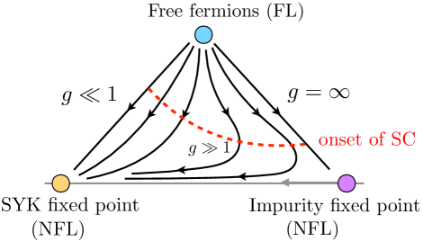
Figure 2: Renormalization group flow that summarizes the physics of the phase diagram of Fig.1. The free-fermion fixed point is always unstable and flows at low energies to the quantum-critical SYK fixed point. At strong coupling, the flow is influenced for a large energy window by a new strong coupling fixed point of fully incoherent fermions. At $g=\infty$ this impurity-like fixed point is stable and governs the behavior at all scales. Superconductivity, marked by the red line, at strong coupling occurs in the vicinity of the impurity-like fixed point. At weak coupling it sets in at the crossover between the two fixed points.

III.1 Low-temperature behavior: quantum-critical SYK-fixed point

We first discuss the solution of this coupled set of equations at low temperatures. The key finding is the following form of the fermionic and bosonic propagators on the Matsubara axis:

$$G\left(\epsilon_{n}\right) = \frac{1}{i\epsilon_{n}\left(1+c_{1}\left|\frac{g^{2}}{\epsilon_{n}}\right|^{2\Delta}\right)},$$ (16)

$$D\left(\nu_{n}\right) = \frac{1}{\nu_{n}^{2}+\omega_{r}^{2}+c_{3}\left|\frac{\nu_{n}}{g^{2}}\right|^{4\Delta-1}},$$ (17)

Here

$$\omega_{r}^{2}=c_{2}\left(T/g^{2}\right)^{4\Delta-1}$$ (18)

is the renormalized phonon frequency. The $c_{i}$ are numerical coefficients of order unity. The value of the exponent $\Delta$ is generally confined to the interval $\frac{1}{4}<\Delta<\frac{1}{2}$, and for our problem we find

$$\Delta\backsimeq 0.420374134464041.$$ (19)

In Appendix B we derive these results, demonstrate that they agree very well with our numerical solution of Eqs.14 and 15, and give analytic and numeric expressions for the coefficients $c_{i}\left(\Delta\right)$. With $\Delta$ of Eq.19 we find $c_{1}\approx 1.154700$, $c_{2}\approx 0.561228$, and $c_{3}\approx 0.709618$.

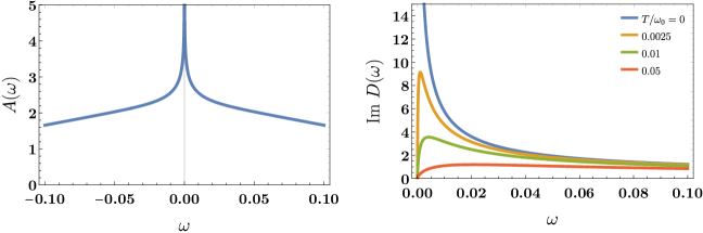
Figure 3: Spectral function $A(\omega)=-\frac{1}{\pi}{\rm Im}G(\omega)$ and imaginary part of the bosonic propagator on the real frequency axis for dimensionless coupling constant $g=0.5$. The phonon spectrum is shown for several temperatures, displaying the softening of the phonon mode $\omega_{r}$.

The findings of Eqs.16, 17, and 18 are summarized in Fig.3, where these equations have been analytically continued from the imaginary to the real frequency axis. Let us discuss the main implications of these findings. The fermionic propagator, Eq.16 is similar to solutions of other SYK models and at low energies is dominated by the self energy

$$\Sigma\left(\epsilon_{n}\right)=-i{\rm sign}\left(\epsilon_{n}\right)c_{1}g^{4\Delta}\left|\epsilon_{n}\right|^{1-2\Delta},$$ (20)

with anomalous exponent $\Delta$. Only the numerical value of $\Delta$ is different from what can be found in purely fermionic models. Notice however that we can vary $\Delta$ in the intervals $\left(\frac{1}{4},\frac{1}{2}\right)$ if we vary the ratio $M/N$ of the number of bosonic and fermionic degrees of freedom, see Appendix C and Ref.Bi2017 . The bosonic propagator Eq.17 is, at low frequencies, dominated by an anomalous Landau damping term, caused by the coupling to fermions and hence determined by the same anomalous exponent $\Delta$.

Notice that the system is critical for all values of $\omega_{0}$ and $g$. This is a surprising result. The renormalized phonon frequency

$$\omega_{r}^{2}=\omega_{0}^{2}-\Pi\left(0\right)$$ (21)

in Eq.18 always vanishes as $T\rightarrow 0$. One might have expected that $\Pi\left(0\right)$ compensates the bare mass only for one specific value of the coupling constant $g$, which would then determine a quantum-critical point. Instead, the system remains critical for all values of $g$, i.e. the fixed point described by Eqs.16 and 17 is stable, see Fig.2. This stability is a consequence of the diverging charge susceptibility of bare fermions with $G\left(i\epsilon_{n}\right)^{-1}\approx i\epsilon_{n}$. It is the Non-Fermi liquid state that lifts the degeneracy of the local Fermi liquid and protects the system against diverging charge fluctuations.

The scaling solution in Eqs. (16) and (17) is valid in a low-temperature regime $T\lesssim T^{*}$ where the self-energies dominate the bare fermion and boson Green’s functions. We can estimate this crossover temperature as

$$T^{*}=\min(T_{f},T_{b}),$$ (22)

where $T_{f}\sim g^{2}\omega_{0}$ and $T_{b}\sim g^{-\phi}\omega_{0}$, where $0<\phi=\frac{8\Delta-2}{3-4\Delta}\leq 2$ for the allowed values $\frac{1}{4}<\Delta\leq\frac{1}{2}$. Below we will see that the relevant exponent at large $g$ is $\Delta=\frac{1}{2}$, so that $\phi=2$. Thus, the SYK-like quantum critical regime is confined to temperatures $T\lesssim g^{2}\omega_{0}$ at small $g$ and $T\lesssim g^{-2}\omega_{0}$ at large $g$ (see Fig. 1).

III.2 Intermediate-temperature behavior: impurity-like Non-Fermi liquid fixed point

The quantum critical regime of Eqs.16 and 17 is however not the only universal Non-Fermi liquid regime of this model. Once $g>1$ an increasingly wide intermediate temperature window $g^{-2}<T<g^{2}$ opens up. In this new temperature window we find for the electron and phonon propagators the solution

$$G\left(\epsilon_{n}\right) = \frac{-2i{\rm sign}\left(\epsilon_{n}\right)}{\sqrt{\epsilon_{n}^{2}+\Omega_{0}^{2}}+\left|\epsilon_{n}\right|},$$ (23)

$$D\left(\nu_{n}\right) = \frac{1}{\nu_{n}^{2}+\omega_{r}^{2}},$$ (24)

with a large fermionic energy scale $\Omega_{0}=\frac{16}{3\pi}g^{2}$ and small phonon energy

$$\omega_{r}^{2}=\left(\frac{3\pi}{8}\right)^{2}T/g^{2}.$$ (25)

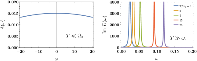
Figure 4: Spectral function and imaginary part of the bosonic propagator on the real frequency axis and for dimensionless coupling constant $g=5$. The phonon spectrum is shown for several temperatures, displaying the softening of the phonon mode $\omega_{r}$.

The findings of Eqs.23, 24, and 25 are summarized in Fig.4. Since $T\ll\Omega_{0}$ fermions are “cold” and effectively behave as if they were quantum-critical with exponent $\Delta=\frac{1}{2}$, i.e. with impurity-like self energy

$$\Sigma\left(\epsilon_{n}\right)=-i{\rm sign}\left(\epsilon_{n}\right)\frac{8}{3\pi}g^{2}.$$ (26)

Non-interacting electrons with static impurities give rise to a similar self energy and can, for a given disorder configuration, be considered a Fermi liquid, essentially by definition. In our case the situation is different. We have to analyze multiple phonon configurations, even for a given disorder configuration of the $g_{ij,k}$. The resulting state cannot be mapped onto a free-fermion problem. Hence the term Non-Fermi liquid. The spectral function $A\left(\omega\right)$ is semicircular with a width $2\Omega_{0}$. The low frequency spectral function is therefore frequency independent

$$A\left(\left|\omega\right|\ll\Omega_{0}\right)=\frac{3}{8g^{2}},$$ (27)

reflecting the incoherent nature of the fermion spectrum, as mentioned in Eq.4 in the introduction. On the other hand, phonons are undamped but “hot”, i.e. thermally excited since $T\gg\omega_{r}$ once $T\gg g^{-2}$. Given the large fermionic energy scale $\Omega_{0}$ we can neglect Landau damping terms that we find to be $\propto\left|\omega_{n}\right|/\Omega_{0}$ in the intermediate energy window. While the phonons are sharp excitations with a strongly renormalized, soft frequency, the fermions are highly incoherent. Similar behavior was discussed in the context of magnetic precursors in cupratesSchmalian1998 ; Schmalian1999 . The impurity-like behavior for the fermionic self energy is expected given the quasi-static nature of the phonons. Notice, all these results correspond to an anomalous fermionic exponent $\Delta=\frac{1}{2}$. This strong-coupling fixed point is unstable and the system eventually crosses over to the low-temperature SYK fixed point. Only for $g=\infty$ does the impurity fixed point describe the ultimate low-$T$ behavior, see Fig.2. The analytic derivation of this strong coupling criticality is summarized in Appendix B and compared with the full numerical solution of Eqs.14 and 15.

IV Superconductivity and Pairing of Non-Fermi Liquids

In the previous section we analyzed the behavior of the model Eq.5 in the normal state. As indicated in Fig.1 the normal state consists of three distinct regions that are separated by crossover lines. Tor $T>T_{f}\approx g^{2}\omega_{0}$ interaction effects are weak and we have essentially free electrons. For $T<T_{f}$ we have two distinct interacting regimes. At lowest temperatures with $T<T^{*}\sim{\rm min}(g^{2}\omega_{0},g^{-2}\omega_{0}$) quantum-critical behavior similar to that found in previous SYK-model calculations occurs, where phonons are characterized by anomalous Landau damping. For strong coupling, i.e. for $g>1$ a new universal intermediate temperature window $g^{-2}<T/\omega_{0}<g^{2}$ opens up where strongly incoherent fermions interact with soft phonons.

Next we allow for superconducting solutions and solve the coupled equations for the normal and anomalous self energies. On the Matsubara axis, these coupled equations are

$$i\epsilon_{n}\left(1-Z\left(\epsilon_{n}\right)\right) = -\bar{g}^{2}T\sum_{n^{\prime}}\frac{D\left(\epsilon_{n}-\epsilon_{n^{\prime}}\right)i\epsilon_{n^{\prime}}Z\left(\epsilon_{n^{\prime}}\right)}{\left(\epsilon_{n^{\prime}}Z\left(\epsilon_{n^{\prime}}\right)\right)^{2}+\Phi\left(\epsilon_{n^{\prime}}\right)^{2}},$$

$$\Phi\left(\epsilon_{n}\right) = \bar{g}^{2}T\sum_{n^{\prime}}\frac{D\left(\epsilon_{n}-\epsilon_{n^{\prime}}\right)\Phi\left(\epsilon_{n^{\prime}}\right)}{\left(\epsilon_{n^{\prime}}Z\left(\epsilon_{n^{\prime}}\right)\right)^{2}+\Phi\left(\epsilon_{n^{\prime}}\right)^{2}}$$

$$\Pi(\nu_{n}) = -2\bar{g}^{2}T\sum_{n^{\prime}}[G(\epsilon_{n^{\prime}}+\nu_{n})G(\epsilon_{n^{\prime}})-F(\epsilon_{n^{\prime}}+\nu_{n})F(\epsilon_{n^{\prime}})].$$ (28)

If we linearize the second equation with respect to the anomalous self energy $\Phi$ and set $\Phi=0$ in the first equation we can determine the superconducting transition temperature. The result of this analysis is summarized in Fig.5. First, our model does indeed give rise to a superconducting ground state for all values of the coupling constant $g>0$. For small $g$ the transition temperature behaves as

$$T_{c}\left(g\ll 1\right)\approx 0.16g^{2}\omega_{0}.$$ (29)

Thus, while $T_{c}$ at weak coupling is numerically smaller than the crossover scale $T^{*}$ to the quantum critical regime, both temperature scales have the same parametric dependence. We will demonstrate in the next section that indeed superconductivity at $g<1$ occurs near the onset of the low-$T$ quantum critical state. The behavior changes at strong coupling, where we find that

$$T_{c}\left(g\rightarrow\infty\right)\approx 0.11188\omega_{0}$$ (30)

approaches a finite value. In this case we form Cooper pairs deep in the Non-Fermi liquid state. We will analyze the behavior of this new superconducting ground state and demonstrate that it is characterized by a subtle formation of bound states of Cooper pairs with the dynamical pairing field.

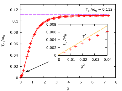
Figure 5: Superconducting transition temperature as function of the coupling constant from the numerical solution of the coupled equations in the normal state and the analysis of the eigenvalue of the pairing vertex. At weak coupling we obtain $T_{c}\propto g^{2}\omega_{0}$ while the transition temperature saturates at strong coupling with $T_{c}\left(g\rightarrow\infty\right)\approx 0.112$$\omega_{0}$.

For our subsequent discussion it is useful to express the pairing state in terms of the gap function

$$\Delta\left(\epsilon_{n}\right)=\Phi\left(\epsilon_{n}\right)/Z\left(\epsilon_{n}\right).$$ (31)

This yields the following coupled equations that are formally equivalent to Eq.28:

$$Z\left(\epsilon_{n}\right) = 1+\bar{g}^{2}T\sum_{n^{\prime}}\frac{D\left(\epsilon_{n}-\epsilon_{n^{\prime}}\right)}{\sqrt{\epsilon_{n^{\prime}}^{2}+\Delta^{2}\left(\epsilon_{n^{\prime}}\right)}}\left[\frac{1}{Z\left(\epsilon_{n^{\prime}}\right)\sqrt{\epsilon_{n^{\prime}}^{2}+\Delta^{2}\left(\epsilon_{n^{\prime}}\right)}}\right]\frac{\epsilon_{n^{\prime}}}{\epsilon_{n}},$$

$$\Delta\left(\epsilon_{n}\right) = \bar{g}^{2}T\sum_{n^{\prime}}\frac{D\left(\epsilon_{n}-\epsilon_{n^{\prime}}\right)}{\sqrt{\epsilon_{n^{\prime}}^{2}+\Delta^{2}\left(\epsilon_{n^{\prime}}\right)}}\left[\frac{1}{Z\left(\epsilon_{n^{\prime}}\right)\sqrt{\epsilon_{n^{\prime}}^{2}+\Delta^{2}\left(\epsilon_{n^{\prime}}\right)}}\right]\left(\Delta\left(\epsilon_{n^{\prime}}\right)-\frac{\epsilon_{n^{\prime}}}{\epsilon_{n}}\Delta\left(\epsilon_{n}\right)\right),$$ (32)

and the same equation for $\Pi(\nu_{n})$. These equations are distinct from the usual Eliashberg theory where the momentum integration over states in a broad band replaces the terms in square brackets by $\pi\rho_{0}$, where $\rho_{0}$ is the density of states in the normal state. In our problem we analyze systems with non-dispering bands, changing the character of the Eliashberg equations. We will see below that for very large $g$ the interactions give rise to a significant broadening of the spectral function that allows to replace the terms in square brackets by a spectral function $A\left(g\rightarrow\infty,\omega\right)=\frac{3}{8}g^{-2}$ times $\pi$. In this limit some known results of the conventional Eliashberg theoryCarbotte1990 ; Allen1975 ; Marsiglio1991 ; Karakozov1991 ; Combescot1995 can be used to obtain a better understanding of the strong coupling limit.

The appeal of the reformulation in terms of the gap function in Eq.32 is that it clearly reveals the role of the zeroth bosonic Matsubara frequency for the gap equation. Suppose the bosonic propagator is dominated by the zeroth Matsubara frequency. This is the case at strong coupling where we obtained with Eqs.24 and 25 that $D\left(\nu_{m}\right)$ is dominated by $\nu_{m}=0$, a result that led to the solutions of Eq.23. From Eq.32 it follows that there is no contribution to the pairing problem for $\epsilon_{n}=\epsilon_{n^{\prime}}$. Thus, static phonons do not affect the onset of superconductivity. The same effect is also responsible for the Anderson theoremAnderson1959 ; Abrikosov1958a ; Abrikosov1958b ; Abrikosov1961 ; Potter2011 ; Kang2016 where static non-magnetic impurities will not affect the superconducting transition temperature. Soft phonons behave somewhat similar to non-magnetic impuritiesMillis1988 ; Abanov2008 . Superconductivity is then only caused by the remaining quantum fluctuations of the phonons. How this happens and what the implications for the spectral properties of the superconducting state are will be discussed in the subsequent sections.

IV.1 Superconductivity at weak coupling

We start our analysis of superconductivity in the weak coupling regime $g<1$ and first estimate the superconducting transition temperature $T_{c}$ from the linearized version of Eq.28

$$\Delta\left(\epsilon_{n}\right)=\bar{g}^{2}T\sum_{n^{\prime}}\frac{D\left(\epsilon_{n}-\epsilon_{n^{\prime}}\right)}{Z\left(\epsilon_{n^{\prime}}\right)\epsilon_{n^{\prime}}^{2}}\left(\Delta\left(\epsilon_{n^{\prime}}\right)-\frac{\epsilon_{n^{\prime}}}{\epsilon_{n}}\Delta\left(\epsilon_{n}\right)\right),$$ (33)

where both $Z\left(\epsilon_{n}\right)$ and $D\left(\nu_{n}\right)$ are determined by our norml state solutions Eq.16 and Eq.17. Here we use $\epsilon_{n}Z\left(\epsilon_{n}\right)=\epsilon_{n}+i\Sigma\left(\epsilon_{n}\right)$. For the phonon propagator of Eq.17 we can safely neglect the $\nu_{n}^{2}$ term in the denominator. When we explicitly write out the temperature dependence in the various terms we obtain the linearized gap equation

$$\Delta\left(\epsilon_{n}\right)=a_{0}\sum_{n^{\prime}}\frac{\left(\frac{T_{f}}{T}\right)^{2\Delta}{\rm sign}\left(\epsilon_{n^{\prime}}\right)}{\left(\frac{T}{T_{f}}\right)^{2\Delta}\left|n^{\prime}+\frac{1}{2}\right|+\left|n^{\prime}+\frac{1}{2}\right|^{1-2\Delta}}\frac{\frac{\Delta\left(\epsilon_{n^{\prime}}\right)}{\epsilon_{n^{\prime}}}-\frac{\Delta\left(\epsilon_{n}\right)}{\epsilon_{n}}}{m_{0}+\left|n-n^{\prime}\right|^{4\Delta-1}},$$

with $m_{0}=\frac{c_{2}}{c_{3}\left(2\pi\right)^{4\Delta-1}}\approx 0.156558$, $a_{0}=\frac{1}{2\pi c_{1}^{2}c_{2}}\approx 0.212687$ and $T_{f}=\frac{1}{2\pi}c_{1}^{\frac{1}{2\Delta}}g^{2}\approx 0.1888g^{2}$. The temperature dependence of the gap equation only occurs in the combination $T/T_{f}$. Thus the scale for the superconducting transition is set by $T_{f}.$ However, this is precisely the temperature scale where the crossover between the univeral low-$T$ non-Fermi liquid fixed point and the high-temperature free fermion behavior takes place. This is also the reason why we included the term $\left(\frac{T}{T_{f}}\right)^{2\Delta}\left|n^{\prime}+\frac{1}{2}\right|$ in the denominator, which corresponds to the bare fermionic propagator. Equally, the coefficient $m_{0}$ occurs as we have to include a finite phonon frequency at the transition temperature. If we keep all those terms we obtain $T_{c}\approx 0.0821g^{2}$. Thus, we find that the transition temperature is about half of the crossover temperature $T_{f}.$ The $g^{2}$ dependence agrees with our numerical finding shown in Fig.5. Not surprisingly, the precise numerical coeffficient in $T_{c}$ cannot be reliably determined as the transition temperature is right in the crossover regime between free-fermion and quantum-critical SYK behavior. The reason is that there appear to be corrections to the fermionic self energy that are formally subleading at low frequencies, yet modify numerical coefficients. The correct behavior was obtained from the full numerical solution and yields Eq.29; see also Fig.5.

This analysis demonstrates that superconductivity in the weak coupling regime occurs at the same temperature scale where quantum critical Non-Fermi liquid behavior emerges. Thus superconductivity occurs instead of the quantum critical regime. While parametrically the same, the numerical coefficient of the transition temperature is somewhat smaller than the crossover scale $T_{f}$ between the region of free fermion and quantum-critical fermion behavior. Thus, in this regime it might be possible to observe quantum critical scaling over a regime up to a decade in frequency or temperature. It should however not be possible to find several decades of universal scaling according to Eqs.16 and 17. Superconductivity prevents such a wide quantum-critical regime.

Nevertheless, it is very intructive to compare our gap function with results from a previous analysis of the linearized gap-equation in quantum-critical systems; see in particular Ref.Abanov2001 ; Chubukov2005 ; Moon2010 ; Metlitski2015 ; Raghu2015 ; Lederer2015 ; Wu2019 . If we formulate the linearized gap equation merely in terms of the universal contributions to the electron and phonon self energies, we obtain

$$\Phi\left(\epsilon_{n}\right)=\frac{T_{c}}{c_{1}^{2}c_{3}}\sum_{n^{\prime}}\frac{\Phi\left(\epsilon_{n^{\prime}}\right)}{\left|\epsilon_{n}-\epsilon_{n^{\prime}}\right|^{4\Delta-1}\left|\epsilon_{n^{\prime}}\right|^{2-4\Delta}},$$ (34)

where $\epsilon_{n}=\left(2n+1\right)\pi T_{c}$. Here we can see explicitly what was discussed in the introduction, namely that the singular pairing interaction $V_{{\rm pair}}\left(\nu_{n}\right)\propto D\left(\nu_{n}\right)\propto\left|\nu_{n}\right|^{1-4\Delta}$ compensates for the less singular fermionic propagator giving rise to a generalized Cooper instability. Self-consistency equations of this type have been discussed in the context of several scenarios for quantum critical pairing in metallic systemsBonesteel1996 ; Son1999 ; Abanov2001 ; Abanov2001b ; Roussev2001 ; Chubukov2005 ; She2009 ; Moon2010 ; Metlitski2015 ; Raghu2015 ; Lederer2015 ; Wu2019 . In this equation the entire $T$-dependence disappears given that the two exponents in the denominator add up to unity. Thus, unless this equation is supplemented by appropriate boundary conditions, it is not possible to determine $T_{c}$, see Ref.Wu2019 . This is essentially achieved by our above solution of the gap equation for $\Delta$_n. For a detailed discussion of the gap-equation in the form Eq.34, see Ref.Moon2010 ; Metlitski2015 ; Raghu2015 ; Lederer2015 ; Wu2019 .

In Fig.6 we show the spectral function in the weak coupling regime at low temperatures that was obtained from a numerical solution of the full coupled equations on the real frequency axis, following the approach of Ref.Langer1995 ; CPC . Our main observation is the emergence of a sharp excitation, and of several high energy structures. We will discuss these high -energy shake-off peaks in greater detail in the discussion of the strong coupling limit. Finally, we observe that in this weak coupling regime the superconducting gap closes as the temperature increases.

Overall, the analysis of the pairing problem in this weak coupling regime closely resembles the behavior that was found in a number of metallic quantum critical pointsBonesteel1996 ; Son1999 ; Abanov2001 ; Abanov2001b ; Roussev2001 ; Chubukov2005 ; She2009 ; Moon2010 ; Metlitski2015 ; Raghu2015 ; Lederer2015 ; Wu2019 . The SYK model proposed here may serve as a starting point to go beyond the mean-field limit and investigate the fluctuation corrections by following the advances in the $1/N$ corrections of SYK-like modelsBagrets2016 ; Bagrets2017 .

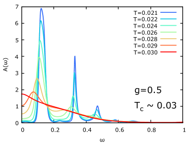
Figure 6: Spectral function as function of temperature for $g=0.5$. The superconducting transition temperature is $T_{c}=0.03\omega_{0}$. We find higher order bound states as well as a gap closing as function of temperature.

IV.2 Superconductivity at strong coupling

The investigation of superconductivity at strong coupling is of particular interest, as it reveals why fully incoherent fermions are able to nevertheless form a coherent superconducting state. We begin again with a determination of the superconducting transition temperature from the linearized gap equation. To this end we start from Eq.32 to obtain

$$\Delta\left(\epsilon_{n}\right)=\frac{3\pi}{8}T_{c}\sum_{n^{\prime}}\frac{1}{\left(\epsilon_{n}-\epsilon_{n^{\prime}}\right)^{2}+\omega_{r}^{2}}\left(\frac{\Delta\left(\epsilon_{n^{\prime}}\right)}{\epsilon_{n^{\prime}}}-\frac{\Delta\left(\epsilon_{n}\right)}{\epsilon_{n}}\right){\rm sign}\left(\epsilon_{n^{\prime}}\right).$$ (35)

Here, we used the normal state result Eq.23 that has the low frequency behavior

$$\left|\epsilon_{n}\right|Z\left(\epsilon_{n}\right)\approx\frac{8}{3\pi}g^{2}.$$ (36)

The large normal state fermionic self energy is responsible for the fact that the coupling constant $g$ gets cancelled in the prefactor of Eq.35. The only dependence on the coupling constant in this equation is in the renormalized phonon frequency $\omega_{r}$. At $T_{c}$, $\omega_{r}$ is determined by the normal state solution of Eq.25. However, since $T\gg\omega_{r}$ in the strong coupling regime and since the zeroth Matsubara frequency does not contribute to superconductivity, we can simply set $\omega_{r}$ to zero in Eq.35. The linearized gap equation becomes

$$\Delta_{n}=\alpha\sum_{n^{\prime}\neq n}\frac{\frac{\Delta_{n^{\prime}}}{2n^{\prime}+1}-\frac{\Delta_{n}}{2n+1}}{\left(2n-2n^{\prime}\right)^{2}}{\rm sign}\left(n^{\prime}+\frac{1}{2}\right)$$ (37)

with $\alpha=\frac{3\omega_{0}^{2}}{8\pi^{2}T_{c}^{2}}$. One easily finds that this equation has a solution for $\alpha_{c}=3.03458$, which yields for the transition temperature $T_{c}=\sqrt{\frac{3\omega_{0}^{2}}{8\pi^{2}\alpha_{c}}}\$. Inserting the numerical coefficients yields Eq.30. The transition temperature saturates as $g\rightarrow\infty$, in quantitative agreement with the numerical results shown in Fig.5. This analysis also reveals the reason why pairing of fully incoherent fermions is possible. The lack of fermionic coherence, with large imaginary part of the electronic self energy, is caused by the coupling to almost static bosonic modes. However, by arguments that in the context of disordered superconductors give rise to the Anderson theorem, such static bosons affect the normal and anomalous self energies $\Sigma$ and $\Phi$, yet they cancel for the actual pairing gap $\Delta=\Phi/Z$ which is solely affected by the much weaker quantum fluctuations of the bosonic spectrum. Thus, pairing of time-reversal partners occurs even for incoherent fermions, a state that is protected by the same mechanism that makes the superconducting transition temperature robust against non-magnetic impuritiesAnderson1959 ; Abrikosov1958a ; Abrikosov1958b ; Abrikosov1961 ; Potter2011 ; Kang2016 ; Millis1988 ; Abanov2008 .

Now that we established that superconductivity sets in at a temperature that is deep in the incoherent strong coupling regime, we discuss the properties of this superconducting state. We start with our numerical results for the spectral function and the anomalous Green’s function. In Fig.7 we show the fermionic spectral function in the superconducting state. In distinction to the gap-closing behavior that occurs at weak coupling, we find a filling of the gap, where the position of the maximum is essentially unchanged with temperature. In addition, higher order shake-off peaks occur that become most evident in the strong coupling limit. The value of the superconducting gap is, just like the transition temperature, independent of coupling constant and of order of the bare phonon frequency $\omega_{0}$. The lowest excitation of the fermions is $\Delta_{0}\approx 0.640869140625\omega_{0}$. This yields

$$2\Delta_{0}/T_{c}\approx 11.456366,$$ (38)

which is more than three times the BCS value $2\pi e^{-\gamma_{E}}\approx 3.527754$. Such large values of $2\Delta_{0}/T_{c}$ have been obtained in the Eliashberg theory at strong coupling and for small phonon frequenciesScalapino1969 ; Carbotte1990 ; for a recent discussion seeWu2019b . Since the spectral weight of the excited state is transferred from energies below the gap, we can estimate the weight of the peak as $Z_{{\rm coh}}\approx\int_{0}^{\Delta\approx\omega_{0}}A_{{\rm ns}}\left(\omega\right)d\omega\propto g^{-2}$, where we used the normal state spectral function of Eq.27. We will see below that this result can be obtained rigorously at large $g$.

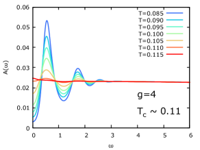
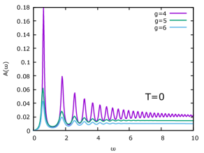
Figure 7: Left panel: spectral function at strong coupling ($g=4$ with $T_{c}\approx 0.11\omega_{0}$) for different temperatures. In distinction to the weak coupling case we find gap filling, rather than gap closing and a pronounced peak-dip-peak structure. The latter is not due to the coupling to the phonon mode, which has much smaller energy. Right panel: spectral function at $T=0$ for different coupling constants revealing a large number of shake-off peaks that reflect the bound state formation in this limit of strongly coupled Cooper pairs. Also, the total weight of the leading coherence peak decreases with increasing coupling strength.

A very intriguing feature of the low-$T$ spectral function is the occurrence of a large number of shake-off peaks at discrete energies $\Omega_{l}$ that are reminiscent of the satellites that emerge as one forms polaronic states due to strong electron-phonon coupling. However, in the conventional polaronic theory these shake-off structures exist at energies $\epsilon_{0}+l\omega_{r}$ where $\epsilon_{0}$ is the bare fermion energy, $\omega_{r}$ the phonon frequencyMahan1993 , and $l$ an integer. In our case $\omega_{r}$ is much smaller than the separation of the peaks in the spectral function. In fact such structures in the normal and anomalous Greens function, see Fig.8, have already been discussed in the context of strong coupling solutions of the Eliashberg theoryMarsiglio1991 ; Karakozov1991 ; Combescot1995 and can be considered as self trapping states of excited quasiparticles in the pairing potential of the other electronsCombescot1995 . The excited quasiparticle polarizes the pairing field, that deforms and traps it. The positions of the peaks are not equidistant. Following Ref.Combescot1995 we find at large $l$ that the energies grow as $\Omega_{l}\approx\frac{\sqrt{3}\pi}{4}\sqrt{2l-1}\omega_{0}$. The first ten peaks are located at $\Omega_{l}=p_{l}\Delta_{0}$ with $p_{l}=(1.,2.81,4.05,5.00,5.76,6.47,7.14,7.71,8.29,8.81)$. The first peak corresponds of course to the gap $\Omega_{1}=\Delta_{0}$. These features are a clear sign of the fact that we have strongly interacting Cooper pairs, instead of an ideal gas of such pairs. While most of these shake-off peaks smear out as the temperature increases (see left panel of Fig.7) the first one or two peaks should be visible and serve as potential explanation for the observed peak-dip-hump structures seen in photoemission spectroscopy measurements of cuprate superconductors near the antinodal momentumDessau1991 ; ZXSchrieffer1997 ; Campuzano1996 ; Fedorov1999 ; Feng2000 .

One way to verify the emergence of these shake-off peaks due to self trapping in the pairing field is via the AC-Josephson effect with current

$$I_{J}\left(t\right)=2et_{0}^{2}\left({\rm Re}\Pi_{F}\left(eV\right)\sin\left(2eVt\right)+{\rm Im}\Pi_{F}\left(eV\right)\cos\left(2eVt\right)\right),$$ (39)

where $\Pi_{F}\left(\omega\right)$ is the retarded version of the Matsubara function $\Pi_{F}\left(\nu_{n}\right)=T\sum_{m}F^{\dagger}\left(\epsilon_{m}\right)F\left(\epsilon_{m}-\nu_{n}\right)$. At low applied voltage $\left|eV\right|<2\Delta_{0}$ the imaginary part of $\Pi_{F}$ vanishes and the Josephson current is proportional to the sinus of the phase differenceJosephson1962 . As the magnitude of the voltage exceeds $2\Delta_{0}$ an additional, phase-shifted AC Josepshon current that is proportional to $\cos(2eVt)$ sets in Harris1974 . The coefficient is proportional to ${\rm Im}\Pi_{F}\left(eV\right)$ that we show in Fig. 9. Clearly the sequence of bound states of the spectral function can be identified in the cosine AC-Josephson response. Most interestingly, the sign change of two consecutive bound states, visible in the anomalous propagator in Fig.8, directly leads to an alternating sign of the phase-shifted Josephson signal. This offers a way to identify the nature of higher energy structures in the spectral function of superconductors, such as the bound states discussed here. For example, peaks in the spectral function due to multiple gaps on different Fermi surface sheets would not display such a sign-changing AC-Josephson signal.

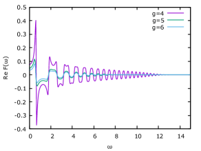
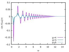
Figure 8: Real part (left panel) and imaginary part (right panel) of the anomalous propagator $F\left(\omega\right)$ at $T=0$ and for different coupling strengths. Notice the alternating sign of the peaks in the imaginary part.

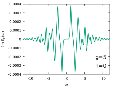
Figure 9: Imaginary part of $\Pi_{F}(\omega)$ (defined in the text) for $g=5$ at $T=0$. ${\rm Im}\Pi_{F}(\omega)$ determines the amplitude of the phase-shifted AC Josephson current at higher voltage. The alternating sign of the peaks shown here is a direct consequence of the sign changes of consecutive peaks in the anomalous propagator, shown in Fig.8. Thus, the AC-Josephson response might serve as a tool to identify the internal structure of the Cooper pair states of a strongly coupled superconductor.

Finally, in Fig.10 we show our results for the softening of the phonon frequency in the superconducting state. In the normal state the phonon mode is expected to soften, first according to Eq.25 and below $T\sim\omega_{0}g^{-2}$ according to Eq. 18. In the normal state $\omega_{r}$ always vanishes for $T\rightarrow 0$. With the onset of superconductivity the phonon frequency still decreases with decreasing $T$, however it reaches a finite value $\omega_{r}^{sc}$ at $T=0$. If we simply determine the phonon renormalization from the high-energy behavior of the spectral function in the superconducting state we find $\omega_{r}^{sc}=\frac{\omega_{0}}{2}\left(\frac{3\pi}{8}\right)^{2}g^{-2}$ which agrees well with our numerical finding. As expected the superconducting ground state has gapped fermion and phonon excitations which explains its coherent nature.

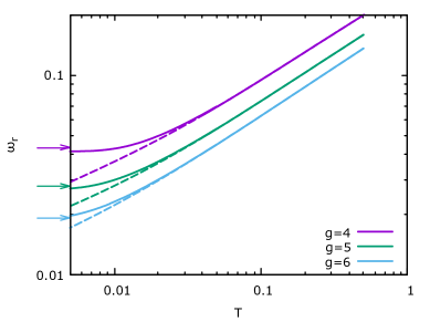
Figure 10: Softening of the phonon frequency in the superconducting state at strong coupling. The dashed line is the normal state result, continued below $T_{c}$. While in the normal state the phonon frequency vanishes as $T\rightarrow 0$, it approaches the finite $T=0$ value $\omega_{r}^{sc}=\frac{\omega_{0}}{2}\left(\frac{3\pi}{8}\right)^{2}g^{-2}$, indicated by the arrows. Thus, both the electrons and the bosons are gapped in the superconducting state.

In the strong coupling limit one can make contact with results that were obtained in the context of the usual Eliashberg theory, where conduction electrons with a large bandwidth require momentum averagingEliashberg1960 ; Scalapino1969 ; Carbotte1990 . This additional momentum integration is not present in the SYK model, where one is interested in the behavior of strongly-interacting narrow bands. From a purely technical point of view, the effect of the momentum integration in the usual Eliashberg formalism is to replace the term

$${\cal A}\left(\epsilon_{n}\right)=\frac{1}{\pi}\frac{1}{Z\left(\epsilon_{n}\right)\sqrt{\epsilon_{n}^{2}+\Delta^{2}\left(\epsilon_{n}\right)}},$$ (40)

that occurs in square brackets in Eq.32, by the normal state density of states of the system. We will now show that at strong coupling the interaction-induced broadening plays a similar role to the momentum integration and we can replace ${\cal A}\left(\epsilon_{n}\right)$ by the broad spectral function of Eq.27, i.e. ${\cal A}\left(\epsilon_{n}\right)\approx\frac{3}{8}g^{-2}$. To demonstrate this we take the $T=0$ limit for $Z\left(\epsilon\right)$ in Eq.32:

$$Z\left(\epsilon\right)=1+\bar{g}^{2}\int\frac{d\epsilon^{\prime}}{2\pi}\frac{1}{\left(\epsilon-\epsilon^{\prime}\right)^{2}+\left(\omega_{r}^{sc}\right)^{2}}\frac{1}{Z\left(\epsilon^{\prime}\right)\left(\epsilon^{\prime 2}+\Delta^{2}\left(\epsilon^{\prime}\right)\right)}\frac{\epsilon^{\prime}}{\epsilon},$$ (41)

At large $g$ the $T=0$ phonon frequency is small and the sharp Lorentzian behaves as a $\delta$-function. Using our above result for $\omega_{r}^{sc}$ it follows that

$$Z\left(\epsilon\right)=1+\left(\frac{8g^{2}}{3\pi}\right)^{2}\frac{1}{Z\left(\epsilon\right)\left(\epsilon{}^{2}+\Delta^{2}\left(\epsilon\right)\right)},$$ (42)

which yields at large $g$ the solution

$$Z\left(\epsilon\right)=\frac{8g^{2}}{3\pi}\frac{1}{\sqrt{\epsilon{}^{2}+\Delta^{2}\left(\epsilon\right)}}.$$ (43)

Thus, while $Z\left(\epsilon\right)$ and $\Delta\left(\epsilon\right)$ depend strongly on frequency in the superconducting state, the combination that enters ${\cal A}\left(\epsilon\right)$ is a constant. We have verified that this result for $Z\left(\epsilon\right)$ agrees very well with the full numerical solution for $g\gtrsim 4$. Using Eq.43 the equation for the gap function is given as

$$\Delta\left(\epsilon_{n}\right)=\frac{3\pi}{8}T\sum_{n^{\prime}}\frac{D\left(\epsilon_{n}-\epsilon_{n^{\prime}}\right)}{\sqrt{\epsilon_{n^{\prime}}^{2}+\Delta^{2}\left(\epsilon_{n^{\prime}}\right)}}\left(\Delta\left(\epsilon_{n^{\prime}}\right)-\frac{\epsilon_{n^{\prime}}}{\epsilon_{n}}\Delta\left(\epsilon_{n}\right)\right).$$ (44)

While the physics we are describing is rather different, formally this equation is identical to the usual Eliashberg theory, yet with a dimensionless coupling constant $\lambda=\frac{3}{8}$ and a very soft phonon frequency. If we set this phonon frequency to zero, the solution for $\Delta\left(\epsilon_{n}\right)$ is fully universal and independent of the coupling constant. Comparing with the numerical solution, we find that for $g\gtrsim 4$ this is indeed the case with high accuracy. Our result Eq.30 can also be obtained from the well known strong coupling solution $T_{c}\approx 0.1827$$\sqrt{\lambda}\omega_{0}$ by Allen and DynesAllen1975 if one inserts $3/8$ for the coupling constant. This is curious as one is very far from the applicability of this strong-coupling Allen-Dynes result for $\lambda=0.375$. The reason we can apply this formula is because of the extreme softening of the phonons in our critical system. In the usual Eliashberg formalism the frequency that enters the phonon propagator $D\left(\nu_{n}\right)$ is the bare, unrenormalized phonon frequency $\omega_{0}$. Then, the Allen Dynes limit of $T_{c}$ only becomes relevant for extremely large values of the couplig constant.

Using Eq.43 we can also find a very efficient way to relate the function $\Delta\left(\omega\right)$ on the real frequency axis and the spectral function

$$A\left(\omega\right)=\frac{3}{8g^{2}}{\rm Re\left(\frac{\omega}{\sqrt{\omega^{2}-\Delta\left(\omega\right)^{2}}}\right)}.$$ (45)

Since at large $g$ the solution for the gap function is independent of the coupling constant, we immediately see that the weight of the superconducting coherence peak must scale as $g^{-2}$, a behavior that we estimated earlier based on the conservation of spectral weight. Thus, the key effect of the incoherent nature of the normal state is the reduced weight of the coherence peak, not its lifetime.

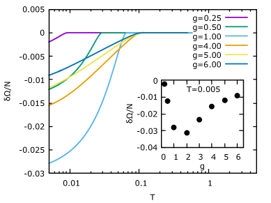
Figure 11: Condensation energy $\delta\Omega/N$ as a function of temperature $T$ for several values of $g$. The inset shows $\delta\Omega/N$ as a function of $g$ at $T=0.005\omega_{0}$.

We finish this discussion with an analysis of the condensation energy as function of temperature and coupling strength. We determine the condensation energy $\delta\Omega$ from the difference of

$$\Omega/N = -T\sum_{n}{\rm tr}\log\left(\hat{1}-\hat{G}_{0}\left(\nu_{n}\right)\hat{\Sigma}\left(\nu_{n}\right)\right)+\frac{T}{2}\sum_{m}\log\left(1-D_{0}\left(\epsilon_{m}\right)\Pi\left(\epsilon_{m}\right)\right),$$ (46)

$$- T\sum_{n}{\rm tr}\left(\hat{G}\left(\nu_{n}\right)\hat{\Sigma}\left(\nu_{n}\right)\right)$$

in the normal and superconductng state. Here, the trace is performed with respect to the degrees of freedom in Nambu space. As shown in Fig. 11, the temperature dependence of the condensation energy is very different in the weak and strong coupling regime with an almost linear behavior for large $g$. In this regime we also find a close relation between the condensation energy and the quasiparticle weight. At weak coupling $g<1$ the magnitude of the condensation energy rises precipitously with increasing $g$. On the other hand, for $g\gtrsim 4$ the magnitude of the condensation energy drops slowly, consistent with the power-law drop off of the quasiparticle weight. Such a correlation between coherent weight in the superconducting state and condensation energy has indeed been observed in the cuprate superconductors Feng2000 .

V Summary

In summary, we introduced and solved a model of interacting electrons and phonons with random, infinite-ranged couplings that is in the class of Sachdev-Ye-Kitaev models and allows for an exact solution in the limit of a large number of fermion and boson flavors. The normal state phase diagram is summarized in Fig. 1 and contains adjacent to a high energy regime of almost free fermions, two distinct Non-Fermi liquid regimes. If the random electron-phonon interaction respects time reversal symmetry not just on the average, but for each disorder configuration, the system becomes superconducting. Despite the incoherent nature of normal state excitations, sharp, coherent excitations, including higher order shake-off peaks, emerge below $T_{c}$. However, the broader the fermionic states above $T_{c}$, the smaller the weight of the coherence peak below $T_{c}$. The superconducting transition temperature grows monotonically with coupling strength and levels off at a finite value that is determined by the bare phonon frequency. We remark that a general upper bound on $T_{c}$ in conventional superconductors was recently proposed in Ref. Esterlis2018 , with the numerical value $T_{c}\lesssim\bar{\omega}/10$ comparable to the maximal $T_{c}$ found here ($\bar{\omega}$ is an appropriately defined maximal phonon frequency). However, in that case the bound is ultimately due to polaron physics at strong coupling, which is absent in the $N\rightarrow\infty$ limit of the model considered here. In contrast to $T_{c}$, we find the condensation energy is non-monotonic and largest for intermediate coupling strength $g\approx 1$. Thus, we expect strong fluctuations for large $g$ if one goes beyond the leading large-$N$ limit. Indeed, the appeal of the SYK formalism is that it offers a well defined avenue to systematically improve the results, see e.g. Refs.Bagrets2016 ; Bagrets2017 . Our analysis can also be used as a starting point for lattice models of coupled strongly-interacting superconductors and may be relevant in the theory of Josephson-Junction arrays that are made up of unconventional superconductors. Finally, our analysis was performed for fermions that interact with a phonon mode, i.e. a scalar boson that couples to the fermion operator $c_{i\sigma}^{\dagger}c_{j\sigma}$ in the charge channel. It is straightforward to generalize the model and include a spin-1 boson $\mathbf{\boldsymbol{\phi}}_{k}$ that couples to electrons via $g_{ij,k}\mathbf{\boldsymbol{\phi}}_{k}\cdot\sum_{\sigma\sigma^{\prime}}c_{i\sigma}^{\dagger}\boldsymbol{\sigma}_{\sigma\sigma^{\prime}}d_{j\mathbf{\sigma^{\prime}}}$ with $\boldsymbol{\sigma}$ the vector of Pauli matrices in spin space and with two fermion species $c_{i\sigma}$ and $d_{j\sigma}$. These two fermion species correspond to different bands or different antinodal regions on the same band, depending on the problem under consideration. The large-$N$ equations of this model are very similar to Eqn.10 and 11, with $\tau_{3}\rightarrow\tau_{0}$. The superconducting gap function of the two fermion species then has a relative minus sign, just like the gap function at the two anti-nodal points of a $d$-wave superconductor. The formal expression for the gap function turns out to be the same as the one discussed in this paper. Overall, the approach presented here is a promising starting point to understand superconductivity in strongly coupled, incoherent materials. It justifies some of the known results of the Eliashberg formalism, in particular in the strong-coupling limit, and serves as a starting point to include fluctuations that go beyond the Eliashberg theory.

Note Added: After the completion of this work, we learned about an independent study of random imaginary coupling between the fermions and bosons by Yuxuan Wang Wang2019 . Because of the distinction in the fermion-boson coupling pairing occurs at higher order in the expansion in $1/N$. However, our normal state results agree with that of Ref.Wang2019 . We are grateful to Y. Wang for sharing his unpublished work with us.

Appendix A Derivation of the Self-Consistency Equations

After performing the disorder average with the help of the replica trick, we obtain for the averaged replicated partition function

$$\overline{Z^{n}}=\int{\cal D}^{n}c^{\dagger}{\cal D}c{\cal D}^{n}\phi e^{-S},$$ (47)

where the action is of the form

$$S=S_{0}+S_{g}.$$ (48)

The bare action is given as

$$S_{0} = \sum_{i\sigma a}\int d\tau c_{i\sigma a}^{\dagger}\left(\tau\right)\left(\partial_{\tau}-\mu\right)c_{i\sigma a}\left(\tau\right)+\sum_{ia}\int d\tau\phi_{ia}\left(\tau\right)\left(-\partial_{\tau}^{2}+m_{0}\right)\phi_{ia}\left(\tau\right)$$ (49)

while the disorder-average induced interaction term is

$$S_{g}=-\frac{g^{2}}{4N^{2}}\sum_{ijk}\left(\sum_{a\sigma}\int d\tau c_{i\sigma a}^{\dagger}\left(\tau\right)c_{j\sigma a}\left(\tau\right)\phi_{ka}\left(\tau\right)+\sum_{a\sigma}\int d\tau c_{j\sigma a}^{\dagger}\left(\tau\right)c_{i\sigma a}\left(\tau\right)\phi_{ka}\left(\tau\right)\right)^{2},$$ (50)

a result that can be rewritten as

$$S_{g} = \frac{g^{2}}{2N^{2}}\sum_{ab\sigma\sigma^{\prime}}\int d\tau d\tau^{\prime}\sum_{i}^{N}\phi_{ia}\left(\tau\right)\phi_{ib}\left(\tau^{\prime}\right)$$ (51)

$$\times \left[\sum_{i}^{N}c_{i\sigma a}^{\dagger}\left(\tau\right)c_{i\sigma^{\prime}b}\left(\tau^{\prime}\right)\sum_{j}^{N}c_{j\sigma^{\prime}b}^{\dagger}\left(\tau^{\prime}\right)c_{j\sigma a}\left(\tau\right)\right.$$

$$- \left.\left(\sum_{i}^{N}c_{i\sigma a}^{\dagger}\left(\tau\right)c_{i\sigma^{\prime}b}^{\dagger}\left(\tau^{\prime}\right)\right)\left(\sum_{j}^{N}c_{j\sigma^{\prime}b}\left(\tau^{\prime}\right)c_{j\sigma a}\left(\tau\right)\right)\right].$$

In order to analyze the action we introduce collective variables $G\left(\tau,\tau^{\prime}\right)$ and Lagrange multiplyer fields $\Sigma\left(\tau,\tau\right)$

$$1 = \int{\cal D}G\prod_{ab\tau\tau^{\prime}}\delta\left(NG_{ba,\sigma^{\prime}\sigma}\left(\tau^{\prime},\tau\right)-\sum_{i}c_{i\sigma a}^{\dagger}\left(\tau\right)c_{i\sigma^{\prime}b}\left(\tau^{\prime}\right)\right)$$ (52)

$$= \int{\cal D}G{\cal D}\Sigma e^{\sum_{ab,\sigma\sigma^{\prime}}\int d\tau d\tau^{\prime}\left(NG_{ba,\sigma^{\prime}\sigma}\left(\tau^{\prime},\tau\right)-\sum_{i}c_{i\sigma a}^{\dagger}\left(\tau\right)c_{i\sigma^{\prime}b}\left(\tau^{\prime}\right)\right)\Sigma_{ab,\sigma\sigma^{\prime}}\left(\tau,\tau^{\prime}\right)},$$

that allow for an efficient decoupling of the interaction terms. Because of the last term in $S_{g}$ we also include corresponding anomalous propagators and self energies:

$$1 = \int{\cal D}F\prod_{ab\tau\tau^{\prime}}\delta\left(NF_{ba,\sigma^{\prime}\sigma}\left(\tau^{\prime},\tau\right)-\sum_{i}c_{i\sigma a}\left(\tau\right)c_{i\sigma^{\prime}b}\left(\tau^{\prime}\right)\right)$$ (53)

$$= \int{\cal D}F{\cal D}\Phi^{+}e^{\sum_{ab,\sigma\sigma^{\prime}}\int d\tau d\tau^{\prime}\left(NF_{ba,\sigma^{\prime}\sigma}\left(\tau^{\prime},\tau\right)-\sum_{i}c_{i\sigma a}\left(\tau\right)c_{i\sigma^{\prime}b}\left(\tau^{\prime}\right)\right)\Phi_{ab,\sigma\sigma^{\prime}}^{+}\left(\tau,\tau^{\prime}\right)},$$

as well as

$$1 = \int{\cal D}F^{+}\prod_{ab\tau\tau^{\prime}}\delta\left(NF_{ba,\sigma^{\prime}\sigma}^{+}\left(\tau^{\prime},\tau\right)-\sum_{i}c_{i\sigma a}^{\dagger}\left(\tau\right)c_{i\sigma^{\prime}b}^{\dagger}\left(\tau^{\prime}\right)\right)$$ (54)

$$= \int{\cal D}F^{+}{\cal D}\Phi e^{\sum_{ab,\sigma\sigma^{\prime}}\int d\tau d\tau^{\prime}\left(NF_{ba,\sigma^{\prime}\sigma}^{+}\left(\tau^{\prime},\tau\right)-\sum_{i}c_{i\sigma a}^{\dagger}\left(\tau\right)c_{i\sigma^{\prime}b}^{\dagger}\left(\tau^{\prime}\right)\right)\Phi_{ab,\sigma\sigma^{\prime}}\left(\tau,\tau^{\prime}\right)}.$$

Finally, for the bosonic degrees of freedom we use:

$$1 = \int{\cal D}D\prod_{ab\tau\tau^{\prime}}\delta\left(ND_{ab}\left(\tau,\tau^{\prime}\right)-\sum_{i}\phi_{ia}\left(\tau\right)\phi_{ib}\left(\tau^{\prime}\right)\right)$$

$$= \int{\cal D}D{\cal D}\Pi e^{\frac{1}{2}\sum_{ab}\int d\tau d\tau^{\prime}\left(ND_{ba}\left(\tau^{\prime},\tau\right)-\sum_{i}\phi_{ia}\left(\tau\right)\phi_{ib}\left(\tau^{\prime}\right)\right)\Pi_{ab}\left(\tau,\tau^{\prime}\right)}$$

and obtain an effective action with a sizable amount of integration variables:

$$\overline{Z^{n}}=\int{\cal D}G{\cal D}\Sigma{\cal D}F^{+}{\cal D}\Phi^{+}{\cal D}F{\cal D}\Phi{\cal D}D{\cal D}\Pi{\cal D}^{n}c^{\dagger}{\cal D}^{n}c{\cal D}\phi e^{-S}$$

where the collective action is now given as

$$S = \sum_{iab\sigma\sigma^{\prime}}\int d\tau d\tau^{\prime}c_{i\sigma a}^{\dagger}\left(\tau\right)\left[\left(\partial_{\tau}-\mu\right)\delta_{ab}\delta_{\sigma\sigma^{\prime}}\delta\left(\tau-\tau^{\prime}\right)+\Sigma_{ab,\sigma\sigma^{\prime}}\left(\tau,\tau^{\prime}\right)\right]c_{i\sigma^{\prime}b}\left(\tau^{\prime}\right)$$

$$+ \sum_{iab\sigma\sigma^{\prime}}\int d\tau d\tau^{\prime}\left[c_{i\sigma a}^{\dagger}\left(\tau\right)\Phi_{ab,\sigma\sigma^{\prime}}\left(\tau,\tau^{\prime}\right)c_{i\sigma^{\prime}b}^{\dagger}\left(\tau^{\prime}\right)+c_{i\sigma a}\left(\tau\right)\Phi_{ab,\sigma\sigma^{\prime}}^{+}\left(\tau,\tau^{\prime}\right)c_{i\sigma^{\prime}b}\left(\tau^{\prime}\right)\right]$$

$$+ \frac{1}{2}\sum_{iab}\int d\tau d\tau^{\prime}\phi_{ia}\left(\tau\right)\left[\left(-\partial_{\tau}^{2}+m\right)\delta_{ab}\delta\left(\tau-\tau^{\prime}\right)-\Pi_{ab}\left(\tau,\tau^{\prime}\right)\right]\phi_{ib}\left(\tau^{\prime}\right)$$

$$- N\sum_{ab,\sigma\sigma^{\prime}}\int d\tau d\tau^{\prime}G_{ba,\sigma^{\prime}\sigma}\left(\tau^{\prime},\tau\right)\Sigma_{ab\sigma\sigma^{\prime}}\left(\tau,\tau^{\prime}\right)+\frac{N}{2}\sum_{ab}\int d\tau d\tau^{\prime}D_{ba}\left(\tau^{\prime},\tau\right)\Pi_{ab}\left(\tau,\tau^{\prime}\right)$$

$$- N\sum_{ab,\sigma\sigma^{\prime}}\int d\tau d\tau^{\prime}F_{ba,\sigma^{\prime}\sigma}\left(\tau^{\prime},\tau\right)\Phi_{ab\sigma\sigma^{\prime}}\left(\tau,\tau^{\prime}\right)-N\sum_{ab,\sigma\sigma^{\prime}}\int d\tau d\tau^{\prime}F_{ba,\sigma^{\prime}\sigma}^{+}\left(\tau^{\prime},\tau\right)\Phi_{ab\sigma\sigma^{\prime}}^{+}\left(\tau,\tau^{\prime}\right)$$

$$+ N\frac{g^{2}}{2}\sum_{ab\sigma\sigma^{\prime}}\int d\tau d\tau^{\prime}\left(G_{ab,\sigma\sigma^{\prime}}\left(\tau,\tau^{\prime}\right)G_{ba,\sigma^{\prime}\sigma}\left(\tau^{\prime},\tau\right)-F_{ab,\sigma\sigma^{\prime}}^{+}\left(\tau,\tau^{\prime}\right)F_{ba,\sigma^{\prime}\sigma}\left(\tau^{\prime},\tau\right)\right)D_{ab}\left(\tau,\tau^{\prime}\right).$$ (56)

We use the Nambu spinor

$$\psi_{ia}\left(\tau\right)=\left(c_{i\uparrow a}\left(\tau\right),c_{i\downarrow a}\left(\tau\right),c_{i\uparrow a}^{\dagger}\left(\tau\right),c_{i\downarrow a}^{\dagger}\left(\tau\right)\right)^{T}$$

and rewrite the first two lines of the previous equation as

$$S_{{\rm ferm}}=-\sum_{iab}\int d\tau d\tau^{\prime}\psi_{ia}^{\dagger}\left(\tau\right)\left(\begin{array}[]{cc}G_{0,ab}^{-1}\left(\tau,\tau^{\prime}\right)-\Sigma_{ab}\left(\tau,\tau^{\prime}\right)&\Phi_{ab}\left(\tau,\tau^{\prime}\right)\\ \Phi_{ab}^{+}\left(\tau,\tau^{\prime}\right)&-\tilde{G}_{0,ba}^{-1}\left(\tau^{\prime},\tau\right)+\Sigma_{ba}\left(\tau^{\prime},\tau\right)\end{array}\right)\psi_{ib}\left(\tau^{\prime}\right).$$

Here we introduced the bare propagators

$$G_{0,ab}^{-1}\left(\tau,\tau^{\prime}\right) = -\left(\partial_{\tau}-\mu\right)\delta_{ab}\sigma_{0}\delta\left(\tau-\tau^{\prime}\right),$$

$$\tilde{G}_{0,ab}^{-1}\left(\tau,\tau^{\prime}\right) = -\left(\partial_{\tau}+\mu\right)\delta_{ab}\sigma_{0}\delta\left(\tau-\tau^{\prime}\right).$$

Then we can work with matrices in Nambu space

$$\hat{G}_{0,ab}^{-1}\left(\tau,\tau^{\prime}\right)=\left(\begin{array}[]{cc}G_{0,ab}^{-1}\left(\tau,\tau^{\prime}\right)&0\\ 0&-\tilde{G}_{0,ba}^{-1}\left(\tau^{\prime},\tau\right)\end{array}\right)$$ (57)

and

$$\hat{\Sigma}_{ab}\left(\tau,\tau^{\prime}\right)=\left(\begin{array}[]{cc}\Sigma_{ab}\left(\tau,\tau^{\prime}\right)&\Phi_{ab}\left(\tau,\tau^{\prime}\right)\\ \Phi_{ab}^{+}\left(\tau,\tau^{\prime}\right)&-\Sigma_{ba}\left(\tau^{\prime},\tau\right)\end{array}\right).$$ (58)

Here $\Sigma_{ab}\left(\tau,\tau^{\prime}\right)$ and $\Phi_{ab}\left(\tau,\tau^{\prime}\right)$ etc. are still $2\times 2$ matrices in spin space. In addition we use for the bare phonon propagator

$$D_{0}^{-1}\left(\tau,\tau^{\prime}\right) = \left(-\partial_{\tau}^{2}+m\right)\delta\left(\tau-\tau^{\prime}\right).$$ (59)

We can now integrate out the fermions and bosons:

$$S = -N{\rm tr}\log\left(\hat{G}_{0}^{-1}-\hat{\Sigma}\right)+\frac{N}{2}{\rm tr}\log\left(D_{0}^{-1}\left(\tau,\tau^{\prime}\right)\delta_{ab}-\Pi_{ab}\left(\tau,\tau^{\prime}\right)\right)$$ (60)

$$- N\sum_{ab,\sigma\sigma^{\prime}}\int d\tau d\tau^{\prime}G_{ba,\sigma^{\prime}\sigma}\left(\tau^{\prime},\tau\right)\Sigma_{ab\sigma\sigma^{\prime}}\left(\tau,\tau^{\prime}\right)+\frac{N}{2}\sum_{ab}\int d\tau d\tau^{\prime}D_{ba}\left(\tau^{\prime},\tau\right)\Pi_{ab}\left(\tau,\tau^{\prime}\right)$$

$$- N\sum_{ab,\sigma\sigma^{\prime}}\int d\tau d\tau^{\prime}F_{ba,\sigma^{\prime}\sigma}\left(\tau^{\prime},\tau\right)\Phi_{ab\sigma\sigma^{\prime}}\left(\tau,\tau^{\prime}\right)-N\sum_{ab,\sigma\sigma^{\prime}}\int d\tau d\tau^{\prime}F_{ba,\sigma^{\prime}\sigma}^{+}\left(\tau^{\prime},\tau\right)\Phi_{ab\sigma\sigma^{\prime}}^{+}\left(\tau,\tau^{\prime}\right)$$

$$+ N\frac{g^{2}}{2}\sum_{ab\sigma\sigma^{\prime}}\int d\tau d\tau^{\prime}\left(G_{ab,\sigma\sigma^{\prime}}\left(\tau,\tau^{\prime}\right)G_{ba,\sigma^{\prime}\sigma}\left(\tau^{\prime},\tau\right)-F_{ab,\sigma\sigma^{\prime}}^{+}\left(\tau,\tau^{\prime}\right)F_{ba,\sigma^{\prime}\sigma}\left(\tau^{\prime},\tau\right)\right)D_{ab}\left(\tau,\tau^{\prime}\right).$$

We assume a replica-diagonal structure such that $\overline{Z^{n}}=\overline{Z}^{n}$. Thus, the average is essentially an annealed one. Now the replica structure disappears from the action that determines $\overline{Z}$:

$$S = -N{\rm tr}\log\left(\hat{G}_{0}^{-1}-\hat{\Sigma}\right)+\frac{N}{2}{\rm tr}\log\left(D_{0}^{-1}-\Pi\right)$$ (61)

$$- N\sum_{\sigma\sigma^{\prime}}\int d\tau d\tau^{\prime}G_{\sigma^{\prime}\sigma}\left(\tau^{\prime},\tau\right)\Sigma_{\sigma\sigma^{\prime}}\left(\tau,\tau^{\prime}\right)+\frac{N}{2}\int d\tau d\tau^{\prime}D\left(\tau^{\prime},\tau\right)\Pi\left(\tau,\tau^{\prime}\right)$$

$$- N\sum_{\sigma\sigma^{\prime}}\int d\tau d\tau^{\prime}F_{\sigma^{\prime}\sigma}\left(\tau^{\prime},\tau\right)\Phi_{\sigma\sigma^{\prime}}^{+}\left(\tau,\tau^{\prime}\right)-N\sum_{\sigma\sigma^{\prime}}\int d\tau d\tau^{\prime}F_{\sigma^{\prime}\sigma}^{+}\left(\tau^{\prime},\tau\right)\Phi_{\sigma\sigma^{\prime}}\left(\tau,\tau^{\prime}\right)$$

$$+ N\frac{g^{2}}{2}\sum_{\sigma\sigma^{\prime}}\int d\tau d\tau^{\prime}\left(G_{\sigma\sigma^{\prime}}\left(\tau,\tau^{\prime}\right)G_{\sigma^{\prime}\sigma}\left(\tau^{\prime},\tau\right)-F_{\sigma\sigma^{\prime}}^{+}\left(\tau,\tau^{\prime}\right)F_{\sigma^{\prime}\sigma}\left(\tau^{\prime},\tau\right)\right)D\left(\tau,\tau^{\prime}\right).$$

At large $N$ we can perform the saddle point approximation and obtain the stationary equations

$$G\left(\tau,\tau^{\prime}\right) = \left(G_{0}^{-1}-\Sigma\right)_{\tau,\tau^{\prime}}^{-1},$$

$$D\left(\tau,\tau^{\prime}\right) = \left(D_{0}^{-1}-\Pi\right)_{\tau,\tau^{\prime}}^{-1},$$

$$\Sigma_{\sigma\sigma^{\prime}}\left(\tau,\tau^{\prime}\right) = g^{2}G_{\sigma\sigma^{\prime}}\left(\tau,\tau^{\prime}\right)D\left(\tau,\tau^{\prime}\right),$$

$$\Phi_{\sigma\sigma^{\prime}}\left(\tau,\tau^{\prime}\right) = -g^{2}F_{\sigma\sigma^{\prime}}\left(\tau^{\prime},\tau\right)D\left(\tau,\tau^{\prime}\right),$$

$$\Pi\left(\tau,\tau^{\prime}\right) = -g^{2}\sum_{\sigma\sigma^{\prime}}\left(G_{\sigma\sigma^{\prime}}\left(\tau^{\prime},\tau\right)G_{\sigma^{\prime}\sigma}\left(\tau,\tau^{\prime}\right)-F_{\sigma\sigma^{\prime}}^{+}\left(\tau^{\prime},\tau\right)F_{\sigma\sigma^{\prime}}\left(\tau,\tau^{\prime}\right)\right).$$ (62)

If we focus on singlet pairing we have $F_{\sigma\sigma^{\prime}}\left(\tau\right)=F\left(\tau\right)i\sigma_{\sigma\sigma^{\prime}}^{y}$ and $F_{\sigma\sigma^{\prime}}^{+}\left(\tau\right)=-F^{+}\left(\tau\right)i\sigma_{\sigma\sigma^{\prime}}^{y}$. Now we can rewrite these equations in the usual fashion in $2\times 2$ Nambu space with $\left(c_{i\uparrow},c_{i\downarrow}^{\dagger}\right)$ with fermionic Green’s function

$$\hat{G}\left(\omega_{n}\right)^{-1}=i\omega_{n}\tau_{0}+\mu\tau_{3}-\hat{\Sigma}\left(\omega_{n}\right).$$ (63)

For the bosons we use

$$D\left(\nu_{n}\right)=\frac{1}{\nu_{n}^{2}+\omega_{0}^{2}+\Pi\left(\nu_{n}\right)}.$$ (64)

Then, the self energies are given as

$$\hat{\Sigma}\left(\tau\right) = g^{2}\tau_{3}\hat{G}\left(\tau\right)\tau_{3}D\left(\tau\right)$$

$$\Pi\left(\tau\right) = -g^{2}{\rm tr}\left(\tau_{3}\hat{G}\left(\tau\right)\tau_{3}\hat{G}\left(-\tau\right)\right).$$ (65)

Those are the coupled equations given above.

Appendix B Derivation of the normal-state results

In this appendix we summarize the derivation of the electron and phonon propagators for the two normal-state regimes. We start our analysis with the behavior in the low-temperature quantum critical SYK-regime and continue with the intermediate temperature impurity-like behavior at strong coupling. In addition to the analytic derivation we also present results of the full numerical solution that confirm our analytic findings in detail.

B.1 Quantum-critical SYK fixed point: derivation of Eqs.16, 17, and 18 and numerical results

We start our analysis at $T=0$ and make the following ansatz for the fermionic self energy

$$\Sigma\left(\omega\right)=-i\lambda{\rm sign}\left(\omega\right)\left|\omega\right|^{1-2\Delta}.$$ (66)

To preserve causality, the coefficient $\lambda$ has to be positive. This is most transparent if one analytically continues this ansatz to the real frequency axis. Here, causality requires that the retarded self energy has a negative imaginary part. With ${\rm Im}\Sigma^{R}\left(\epsilon\right)=-\sin\left(\pi\Delta\right)\lambda\left|\epsilon\right|^{\eta}$ follows $\lambda>0$ for $0<\Delta<1$.

As long as $\Delta>0$ the low-energy fermionic Green’s function is dominated by this singular self energy

$$G\left(\omega\right) \approx -\frac{1}{\Sigma\left(\omega\right)}=-\frac{i}{\lambda}{\rm sign}\left(\omega\right)\left|\omega\right|^{-\left(1-2\Delta\right)}.$$ (67)

On the real axis this corresponds to the spectral function $A\left(\epsilon\right)=-\frac{1}{\pi}{\rm Im}G^{R}\left(\epsilon\right)=\frac{\sin\left(\pi\Delta\right)\left|\epsilon\right|^{-\left(1-2\Delta\right)}}{\lambda\pi}$ . The bosonic self energy is

$$\Pi\left(\Omega\right) = -2\bar{g}^{2}\int\frac{d\omega}{2\pi}G\left(\omega\right)G\left(\omega+\Omega\right)$$ (68)

$$= \frac{2g^{2}}{\lambda^{2}}\int\frac{d\omega}{2\pi}\frac{{\rm sign}\left(\omega\right){\rm sign}\left(\omega+\Omega\right)}{\left|\omega\right|^{1-2\Delta}\left|\omega+\Omega\right|^{1-2\Delta}}$$

This bosonic self energy for $\Omega-0$ is ultraviolet divergent if $\Delta>\frac{1}{4}$, i.e. $\Pi\left(0\right)\propto\Lambda^{4\Delta-1}$ with upper cut-off $\Lambda$. This divergency can be avoided if we include the full propagator and write

$$\Pi\left(0\right) = -2\bar{g}^{2}\int\frac{d\omega}{2\pi}G\left(\omega\right)^{2}=-2g^{2}\int\frac{d\omega}{2\pi}\left(\frac{1}{i\omega-\Sigma\left(\omega\right)}\right)^{2}$$ (69)

$$= \frac{2\Delta-1}{2\Delta^{2}\sin\frac{\pi}{2\Delta}}\bar{g}^{2}\lambda^{-\frac{1}{2\Delta}}.$$

Next we analyze the dynamic part $\delta\Pi\left(\Omega\right)=\Pi\left(\Omega\right)-\Pi\left(0\right)$. It is easiest to do this by first Fourier transforming the propagator to imaginary time:

$$G\left(\tau\right)=-\frac{\Gamma\left(2\Delta\right)\sin\left(\pi\Delta\right)}{\pi\lambda}\frac{{\rm sign}\left(\tau\right)}{\left|\tau\right|^{2\Delta}}.$$ (70)

such that the Fourier transform of the phonon self energy is given as $\Pi\left(\tau\right)=2g^{2}\left(\frac{\Gamma\left(2\Delta\right)\sin\left(\pi\Delta\right)}{\pi\lambda}\right)^{2}\frac{1}{\left|\tau\right|^{4\Delta}}$, which yields

$$\delta\Pi\left(\omega\right) = 2\int_{0}^{\infty}\Pi\left(\tau\right)\left(\cos\left(\omega\tau\right)-1\right)d\tau$$

$$= -\frac{g^{2}}{\lambda^{2}}C_{\Delta}\left|\omega\right|^{4\Delta-1}$$

with coefficient $C_{\Delta}=-8\cos\left(\pi\Delta\right)\sin^{3}\left(\pi\Delta\right)\Gamma\left(2\Delta\right)^{2}\Gamma\left(1-4\Delta\right)/\pi^{2}.$

Now we can analyze the bosonic propagator $D\left(\Omega\right).$ We can neglect the bare $\Omega^{2}$ term against the singular bosonic frequency dependence due to the Landau damping. In addition we can only expect a power law solution if indeed $\omega_{0}^{2}-\Pi\left(0\right)=0$. If this is the case, it follows for the bosonic propagator

$$D\left(\Omega\right)\approx-\frac{1}{\delta\Pi\left(\Omega\right)}=\frac{\lambda^{2}}{\bar{g}^{2}C_{\Delta}}\left|\Omega\right|^{1-4\Delta}.$$ (71)

The Fourier transform is $D\left(\tau\right)=\frac{\lambda^{2}}{g^{2}}B_{\Delta}\frac{1}{\left|\tau\right|^{2-4\Delta}}$with $B_{\Delta}=\frac{\pi\left(1-4\Delta\right)\cos\left(2\pi\Delta\right)}{8\Gamma\left(2\Delta\right)^{2}\cos\left(\pi\Delta\right)\sin^{3}\left(\pi\Delta\right)}$ which gives for the self energy

$$\Sigma\left(\tau\right)=-\lambda\frac{B_{\Delta}\Gamma\left(2\Delta\right)\sin\left(\pi\Delta\right)}{\pi}\frac{{\rm sign}\left(\tau\right)}{\left|\tau\right|^{2-2\Delta}}.$$ (72)

Fourier transforming this back to the Matsubara frequency axis finally yields

$$\Sigma\left(\omega\right)=-i\lambda A_{\Delta}{\rm sign}\left(\omega\right)\left|\omega\right|^{1-2\Delta}$$ (73)

with

$$A_{\Delta}=\frac{4\Delta-1}{2\left(2\Delta-1\right)\left(\sec\left(2\pi\Delta\right)-1\right)}.$$ (74)

Notice, for the Fourier transforms to be well defined, it must hold that $\frac{1}{4}<\Delta<\frac{1}{2}$. In order to have a self consistent solution it must of course hold that $A_{\Delta}=1$. This determines the exponent $\Delta$ given in Eq. 19. Interestingly, The coefficient $\lambda$ remains undetermined by this procedure. However, our solution still relies on the assumption that the renormalized phonon frequency vanishes at $T=0$. We have not yet determined when this is the case. We can now always use the freedom and determine $\lambda$ such that $\omega_{r}\left(T=0\right)=0$, which yields the condition

$$\lambda=c_{1}g^{4\Delta}$$ (75)

in order to generate a critical state for all values of the coupling constant. The numerical coefficient is

$$c_{1}=\left(\frac{2\Delta-1}{2\Delta^{2}\sin\frac{\pi}{2\Delta}}\right)^{2\Delta}.$$ (76)

With $\Delta$ from Eq. 19 follows $c_{1}\approx 0.8322602114$. There is one caveat in this argumentation. The relationship between $\Pi(0)$ and $\lambda$ that we used to determine the coefficient $c_{1}$ relied on the simultaneous knowledge of the low and high-frequency behavior of the fermionic propagator, see Eq. 69. To address this, we used an expression that interpolates between the two known limits. Such an approach gives the correct qualitative behavior. Yet the numerical value for $c_{1}$ cannot be reliably determined by such a procedure. To avoid this uncertainty we determined this coefficient from the full numerical solution of the problem that confirms our scaling results in detail; see below. This yields $c_{1}\approx 1.1547005$ which is somewhat larger than the above estimate. In what follows we will use this result for $c_{1}$. Notice, all other coefficients of our analysis, such as $C_{\Delta}$ or $A_{\Delta}$ can be uniquely determined by the universal low-energy behavior and do not have to be determined numerically.

These results for the phonon frequency allow us to determine the coefficient of the dynamic part of the boson propagator

$$\delta\Pi\left(\omega\right)=-c_{3}\left|\frac{\omega}{g^{2}}\right|^{4\Delta-1}$$ (77)

where $c_{3}=\frac{C_{\Delta}}{c_{1}^{2}}$. With $\Delta$ from Eq. 19 and the numerically determined value of $c_{1}$ follows $c_{3}\approx 0.709618$.

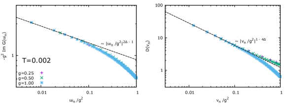
Figure 12: Numerical solution of the fermionic (left panel) and bosonic (right panel) propagators on the imaginary axis in comparison with the analytic solution given in Eqs.16, 17.

This analysis further allows us to determine the temperature dependence of the phonon frequency, which is determined via

$$\omega_{r}^{2}\left(T\right)=\omega_{0}^{2}-\Pi\left(T\right),$$ (78)

where

$$\Pi\left(T\right)=-2g^{2}T\sum_{n=-\infty}^{\infty}G\left(\omega_{n}\right)^{2}.$$ (79)

At low but finite temperatures we use for the propagator our result

$$G\left(\omega_{n}\right)=\frac{1}{i\omega_{n}+i\lambda{\rm sign}\left(\omega_{n}\right)\left|\omega_{n}\right|^{1-2\Delta}}.$$ (80)

Using the Poisson summation formula for fermionic Matsubara sums gives for the phonon frequency

$$\omega_{r}^{2}\left(T\right)=\omega_{0}^{2}-2g^{2}\sum_{k=-\infty}^{\infty}\left(-1\right)^{k}\int_{0}^{\infty}\frac{d\omega}{\pi}\frac{\cos\left(\beta\omega k\right)}{\left(\omega+\lambda\omega^{1-2\Delta}\right)^{2}}$$ (81)

The $k=0$ term corresponds to the $T=0$ result. Thus, it exactly cancels the bare frequency. The remaining frequency integrals are ultraviolet convergent even without the bare fermionic propagator included, which finally gives

$$\omega_{r}^{2}\left(T\right) = \frac{4g^{2}}{\lambda^{2}}\sum_{k=1}^{\infty}\left(-1\right)^{k+1}\int_{0}^{\infty}\frac{d\omega}{\pi}\frac{\cos\left(\beta\omega k\right)}{\omega^{2-4\Delta}}$$ (82)

$$= c_{2}\left(\frac{T}{g^{2}}\right)^{4\Delta-1},$$

with numerical coefficient

$$c_{2}=\frac{4}{\pi c_{1}^{2}}\sin\left(2\pi\Delta\right)\Gamma\left(4\Delta-1\right)\left(1-2^{2-4\Delta}\right)\zeta\left(4\Delta-1\right),$$ (83)

where $c_{1}$ was determined numerically, see text below Eq. 76. With $\Delta$ from Eq. 19 follows $c_{2}\approx 0.561228$.

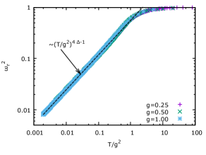
Figure 13: Temperature dependence of the renormalized phonon frequency for several values of the coupling constant $g$ determined from the numerical solution of the coupled equations and compared with the analytical expression of Eq.18.

We finish this discussion with a comparison of our analytical results with the numerical solutions of the coupled equations in the normal state. In Fig.12 we compare the fermionic and bosonic propagators as function of the imaginary Matsubara frequency with our analytic solution of Eqs.16, 17. Finally, In Fig.13 we demonstrate that the phonon frequency agrees with our analytical result Eq.18. In particular this demonstrates that indeed the phonon frequency is soft for all values of $g$.

B.2 Impurity-like fixed point: derivation of Eqs.23, 24 and 25 and numerical results

Let us assume that the boson propagator behaves as in Eq.24 with renormalized boson frequency $\omega_{r}$, but without additional dynamic renormalizations due to Landau damping. We further assume $T\gg\omega_{r}$ something we need to check below to be consistent. Then follows that the self energy is dominated by the lowest bosonic Matsubara frequency, i.e. bosons behave as classical impurities:

$$\Sigma\left(\omega_{n}\right) = g^{2}T\sum_{n^{\prime}}D\left(\omega_{n}-\omega_{n^{\prime}}\right)G\left(\omega_{n^{\prime}}\right)$$ (84)

$$= \frac{g^{2}T}{\omega_{r}^{2}}\frac{1}{i\omega_{n}-\Sigma\left(\omega_{n}\right)}$$

This suggests to introduce the energy scale$\Omega_{0}=2\sqrt{\frac{g^{2}T}{\omega_{r}^{2}}}$which yields

$$\Sigma\left(\omega_{n}\right)=-i{\rm sign}\left(\omega_{n}\right)\frac{1}{2}\left(\sqrt{\omega_{n}^{2}+\Omega_{0}^{2}}-\left|\omega_{n}\right|\right)$$ (85)

as solution of the above quadratic equation. For $\left|\omega_{n}\right|\ll\Omega_{0}$ holds $\Sigma\left(\omega_{n}\right)=-i{\rm sign}\left(\omega_{n}\right)\frac{\Omega_{0}}{2}$ while for large frequencies follows $\Sigma\left(\omega_{n}\right)=-i{\rm sign}\left(\omega_{n}\right)\frac{\Omega_{0}^{2}}{4\left|\omega\right|}$. For the fermionic Green’s function follows then Eq.23. Next we determine the bosonic self energy for this problem:

$$\Pi\left(\omega_{n}\right)=-2g^{2}T\sum_{n^{\prime}}G\left(\omega_{n^{\prime}}\right)G\left(\omega_{n^{\prime}}+\omega_{n}\right).$$ (86)

Let us first determine the zero frequency part

$$\Pi\left(0\right) = -2g^{2}T\sum_{n^{\prime}}G\left(\omega_{n^{\prime}}\right)^{2}$$ (87)

$$= 8g^{2}T\sum_{n^{\prime}}\frac{1}{\left(\sqrt{\omega_{n}^{2}+\Omega_{0}^{2}}+\left|\omega_{n}\right|\right)^{2}}$$

Let us try to determine $\Omega_{0}$ from the condition that the boson frequency goes to zero as $T$ is extrapolated to $T=0$. Formally we can just require that $\Pi\left(0\right)=\omega_{0}^{2}$ at $T=0.$ Then we have ‘

$$\Pi\left(0\right) = 8g^{2}\int_{0}^{\infty}\frac{d\omega}{\pi}\frac{1}{\left(\sqrt{\omega^{2}+\Omega_{0}^{2}}+\omega\right)^{2}}$$ (88)

$$= \frac{16g^{2}}{3\pi\Omega_{0}}$$

This yields $\Omega_{0}=\frac{16}{3\pi}g^{2}$. Combining both expressions that we obtained for $\Omega_{0}$ can be used to determine the phonon frequency and gives rise to our result Eq.25. The assumption of classical bosons was $T\gg\omega_{r}$ which implies $T\gg g^{-2}$, consistent in the strong coupling limit. In addition, as long as $T\ll g^{2}$ we also have $T\ll\Omega_{0}$ and the evaluation of the above fermionic Matsubara sum in the zero-temperature limit is justified. The frequency dependence of the self energy for $\omega\ll g^{2}$ is then$\Sigma\left(\omega_{n}\right)=-i{\rm sign}\left(\omega_{n}\right)\frac{8}{3\pi}g^{2}$.

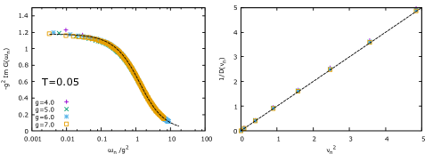
Figure 14: Numerical solution of the fermionic (left panel) and bosonic (right panel) propagators on the imaginary axis in comparison with the analytic solution given in Eqs.23, 24.

For consistency we have to check that we can indeed ignore the frequency dependence of the bosonic self energy. The only scale that enters the fermionic propagator is $\Omega_{0}$. In the relevant limit $T\ll\Omega_{0}$ the fermions are essentially at zero temperature, where

$$\delta\Pi\left(\omega\right) = 2\int_{0}^{\infty}d\tau\Pi\left(\tau\right)\left(\cos\left(\omega\tau\right)-1\right)$$

$$= -4g^{2}\int_{0}^{\infty}d\tau G\left(\tau\right)G\left(-\tau\right)\left(\cos\left(\omega\tau\right)-1\right)$$

The Fourier transform of the fermionic propagator can be determined analytically and expressed in terms of modified Bessel functions and the modified Struve function. For our purposes it suffices to analyze the short and long time limit:

$$G\left(\tau\right)={\rm sign}\left(\tau\right)\times\left\{\begin{array}[]{cc}\frac{1}{\Omega_{0}\left|\tau\right|}&{\rm if}\,\,\left|\tau\right|\gg\Omega_{0}^{-1}\\ \frac{1}{2}-\frac{2}{3\pi}\left|\tau\right|\Omega_{0}&{\rm if}\,\,\left|\tau\right|\ll\Omega_{0}^{-1}\end{array}\right.,$$ (89)

which yields

$$\delta\Pi\left(\omega\right) \approx- \frac{\left|\omega\right|}{\Omega_{0}}.$$

This Landau damping term is negligible compared to $\omega_{n}^{2}$ for $T\gg g^{-2}$. Thus, we can indeed approximate the bosonic propagator by Eq.24.

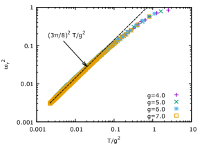
Figure 15: Temperature dependence of the renormalized phonon frequency for several values of the coupling constant $g$ determined from the numerical solution of the coupled equations and compared with the analytical expression of Eq.25.

We finish this discussion with a comparison of our analytical results with the numerical solutions of the coupled equations in the normal state. In Fig.14 we compare the fermionic and bosonic propagators as function of the imaginary Matsubara frequency with our analytic solution of Eqs.23, 24. Finally, In Fig.15 we demonstrate that the phonon frequency agrees with our analytical result Eq.25.

Appendix C On the role of distinct fermion and boson modes

The ratio $m=M/N$ changes the relative importance of the fermion and boson self energies. Changing the ratio $m$ of the number of boson and fermion flavors does not affect the overall behavior of Eqs.10 and 17. The exponent $\Delta$ changes continuously from $\Delta\left(m\rightarrow 0\right)\rightarrow 1/2$ to $\Delta\left(m\rightarrow\infty\right)\rightarrow 1/4$. The phonon softening follows formally still Eq.18, yet the temperature scale below which this powerlaw softening occurs depends sensitively on the relative importance of the phonon and electron renormalizations. If phonon self energy effects dominate ($m\ll 1$) we find $\omega_{r}^{2}=\frac{m}{4}\pi^{2}\log 2\left(T/g^{2}\right)^{1-\frac{m}{2}}$, i.e. phonons are soft below a very large temperature $T^{*}\sim g^{2}/m^{1-\frac{m}{2}}$. In the opposite limit, of large $m$, i.e. relatively negligible phonon self energy, holds that $\omega_{r}^{2}\approx\left(\frac{T}{g^{2}}\right)^{\sqrt{\frac{2}{\pi m}}}$and the temperature window below phonon softening takes place is exponentially small $T^{*}\sim g^{2}e^{-\sqrt{\frac{\pi m}{2}}}$.