Measuring clock jumps using pulsar timing

Abstract

In this paper, we investigate the statistical signal-processing algorithm to measure the instant local clock jump from the timing data of multiple pulsars. Our algorithm is based on the framework of Bayesian statistics. In order to make the Bayesian algorithm applicable with limited computational resources, we dedicated our efforts to the analytic marginalization of irrelevant parameters. We found that the widely used parameter for pulsar timing systematics, the ‘Efac’ parameter, can be analytically marginalized. This reduces the Gaussian likelihood to a function very similar to the Student’s $t$-distribution. Our iterative method to solve the maximum likelihood estimator is also explained in the paper. Using pulsar timing data from the Yunnan Kunming 40m radio telescope, we demonstrate the application of the method, where 80-ns level precision for the clock jump can be achieved. Such a precision is comparable to that of current commercial time transferring service using satellites. We expect that the current method could help developing the autonomous pulsar time scale.

97.60.Gb, 05.45.Tp, 95.55.Sh

1 Introduction

Pulsars are stable celestial clocks, particularly, the long-term stability of millisecond pulsars (MSPs) is comparable to that of the current atomic time-scales [2, 1]. On a short time-scale, the noise in pulsar timing signals becomes signal-to-noise ratio limited, and it is widely accepted that the atomic clock is more stable [1]. At first glance, pulsar timing would not help much, if one focuses on the short term timing stability. Indeed, most of the previous studies aimed at developing a pulsar time-scale with long-term stability [6, 5, 3, 7, 4], while the short-term stability is not extensively investigated.

The traditional local time-frequency sources based on the atomic clock to generate the frequency standard, GPS technology have two major components: (i) a local and (ii) a GPS receiver as a servo to regularize the long-term timing stability [8]. The atomic frequency standard easily reaches a daily Allan variance of $10^{-13}$, while the GPS system performs rather well in time broadcasting, and the precision of 10 ns or better can be achieved using the commercial systems [9]. Clearly, it is unreasonable to expect that pulsar timing will surpass such high stability on short-timescales.

However, the above mentioned stability of the atomic frequency standard is based on the assumption that the atomic frequency standard is well behaved. In practice, due to environmental variations, frequency standard tuning, or other factors (e.g. accidentally changing clock configuration, replacing cables, or interference in the GPS receiver), the local time standard sometimes shows unexpected jitter. In most of the cases, the time signal jumps for a few micro- to milli-seconds. This is a rather common phenomenon, and appears nearly at all astronomical observatories (for an example, see [10]). Clearly, the very first step to construct a standalone pulsar timescale aiming at real scenario applications would be the identification of those signal jitters and related corrections.

In this paper, we propose to use the timing data of multiple pulsars to diagnose and correct such local time jitter. This is very similar to a pulsar timing array (PTA) experiment, which primarily aims at detecting gravitational waves at the nano-Hz band [11]. We introduce the algorithm to compute the local clock jumps from pulsar timing data in Section 2. In Section 3, we demonstrate the algorithm using pulsar timing data from the Kunming 40m (KM40m) radio telescope. The conclusions and discussions are made in Section 4.

2 Waveform estimation for clock jumps

In the common pulsar timing practice, one measures the TOA at the telescope site. The TOA is then converted to the TOA as seen by an observer at the pulsar’s co-rotating reference frame. During the conversion, one accounts for effects such as Earth motion in the Solar system, electromagnetic wave dispersion, pulsar motion with respect to the Solar-system barycenter. The orbital dynamics of the pulsar also need to be corrected, if it is in a binary system. The next step is to compute the pulsar timing residuals. Here, an integer phase is subtracted from the pulsar-frame TOA, and the difference between the TOA and the modeled integer phase is the timing residual. All the unmodeled effects, such as clock jitter, reside in these timing residuals. We refer the interested readers [12] and references therein for an extensive description of pulsar timing techniques.

The clock jitter or jump introduces a common mode in all pulsars’ timing data, i.e. all the TOAs will be late for a given value at the same epoch, if the clock ticking leaps forward. Such a common mode is very different from other possible noise signals, e.g. pulsar intrinsic noise will not be correlated among pulsars. The clock-induced common mode is identical for all pulsars. We need to identify this identical signal and estimate the waveform in order to compute the clock jump.

Our algorithm to extract the clock jump is based on the maximum likelihood estimator (MLE). For the waveform estimation purpose, the MLE was proven to be asymptotically optimal [13]. Such a property guarantees that the error of waveform estimation approaches the best possible values when the signal-to-noise ratio becomes large.

Clock jitter happens on timescales usually less than a few minutes. We can use pulsar timing data around the jitter epoch to determine the clock jitter amplitude. Neglecting the red noise contribution for short timescales, the timing residuals contain mainly two parts, the clock jitter and measurement error, i.e.

$$R_{i,j}=s_{j}+n_{i,j}\,,$$ (1)

where we denote the timing residual of the $i$-th pulsar at the $j$-th epoch as $R_{i,j}$, $s_{i,j}$ is the waveform of the clock jitter and $n_{i,j}$ is the measurement error, following the same convention for the indices as for the timing residual ($R$). The noise ($n_{i,j}$) is a zero mean Gaussian random variable. In this paper, we assume that there are extra systematics in determining the errorbar of each TOA. We summarize the systematics using the ‘Efac’ parameters similar to previous studies [14]. The likelihood for the timing residual thus becomes

$$f(R_{i,j})\propto\prod_{i=1}^{N}\prod_{j=1}^{M_{i}}\frac{1}{\eta_{i}\sigma_{i,j}}e^{-\frac{1}{2}\left(\frac{R_{i,j}-s_{i,j}-\mu_{i}}{\eta_{i}\sigma_{i,j}}\right)^{2}}\,.$$ (2)

Here, the function $f$ is the likelihood function, i.e. the probability density for the given data ($R_{i,j}$). $N$ and $M_{i}$ are the total number of pulsars and epochs for the $i$-th pulsar. $\mu_{i}$ is the local mean of the residual, $\sigma_{i,j}$ is the errorbar of each data point. The ‘Efac’ parameter $\eta_{i}$ is defined for each pulsar to include the minimum practical modeling for the measurement of systematics.

Focusing on the clock jitter, the signal will be identical for all pulsars. We model the clock jitter using a step function of the form

$$s_{i,j}=\left\{\begin{array}[]{l}s_{0},\textrm{for }T_{i,j}>t_{0}\,,\\ 0,\textrm{ for alternatives}\,,\end{array}\right.$$ (3)

where $s_{0}$ is the amplitude of the clock jitter, which allows for both positive and negative values corresponding to the two possible ways of clock jitter, i.e. delay or advance. The time epoch of the data points is described by $T_{i,j}$.

We can now split the likelihood into a multiplication of two independence parts, the one before the clock jitter and the one after it, i.e.

$$f(R_{i,j})\propto\prod_{i=1}^{N}\prod_{j=1}^{\rm before}\frac{1}{\eta_{i}\sigma_{i,j}}e^{-\frac{1}{2}\left(\frac{R_{i,j}-\mu_{i}}{\eta_{i}\sigma_{i,j}}\right)^{2}}\prod_{i=1}^{N}\prod_{j={\rm after}}^{M_{i}}\frac{1}{\eta_{i}\sigma_{i,j}}e^{-\frac{1}{2}\left(\frac{R_{i,j}-s_{0}-\mu_{i}}{\eta_{i}\sigma_{i,j}}\right)^{2}}\,.$$ (4)

By inserting Equation 3 into Equation 4, one can see that the likelihood is controlled by $2+2N$ parameters. There are two parameters for the clock jitter, the event’s amplitude and epoch ($s_{0}$ and $t_{0}$), $N$ pulsar ‘Efac’ parameters ($\eta_{i}$) and finally $N$ local mean values ($\mu_{i}$). The MLEs for all the parameters are derived according to

$${s_{0},t_{0},\mu_{i},\eta_{i}}={\rm argmax}[f(R_{i,j})]\,.$$ (5)

The statistical inference seems to be straightforward, e.g. one can perform Monte-Carlo Bayesian inference with the likelihood function (Equation 4) to measure all $2+2N$ parameters and related errors.

However, for the current problem, such a full Monte-Carlo Bayesian method is not ideal. It has a very high computational cost due to the potentially large number of parameters. On the other hand, the Bayesian method would perform the inference on all parameters, for some of which we are not interested in their values, e.g. $\eta_{i}$ and $\mu_{i}$ are parameters for individual pulsars. Furthermore, we only need to measure the epoch of jitter to the precision of observation cadence due to the sparseness of pulsar timing observations. The requirement for jitter-epoch estimation is rather rough. As we will show in the following paragraphs, it is possible to compute the MLE in a very computationally efficient way, if we perform a one-dimensional search for the jitter epoch ($t_{0}$). That is, we can compute the MLE and error for the clock jump amplitude using a direct method, at each trial jitter epoch.

Since ‘Efac’ parameters are not required, we can marginalize the them by integrating the likelihood function ($f$) under Bayesian prior, and the reduced likelihood ($f^{\prime}$) is then defined as

$$f^{\prime}(R_{i,j})\equiv\int f(R_{i,j})p(\eta)\,{\rm d}\eta\,,$$ (6)

where function $p(\eta)$ is the prior of $\eta$. The least informative prior will be $p(\eta)\propto 1/\eta$, i.e. when the $\eta$ probability distributes uniformly in logarithmic space [15]. Inserting Equation 4 into Equation 6, one can show that

$$f^{\prime}(R_{i,j})\propto\prod_{i=1}^{N}\left[\sum_{j=1}^{\rm before}\left(\frac{R_{i,j}-\mu_{i}}{\sigma_{i,j}}\right)^{2}+\sum_{j={\rm after}}^{M_{i}}\left(\frac{R_{i,j}-\mu_{i}-s_{0}}{\sigma_{i,j}}\right)^{2}\right]^{-M_{i}/2}\,.$$ (7)

The above result is very similar to the Student’s $t$-distribution with $M-1$ degrees of freedom, which describes the mean of a normally distributed population with finite sample size and unknown standard deviation. Note that for any time epoch between two available data points, the data defining ‘before’ and ‘after’ are the same, and as such for all time epochs between these points the likelihood value will be the same. In this way, the best measurement precision for the epoch of clock jump is the length between the two nearest data points containing the jump. This becomes more apparent in case where the jump is associated with data gaps longer than the average data cadence, as we will also see in Section 3.

The MLE for $\mu_{i}$ can be readily computed from $\partial f^{\prime}/\partial\mu_{i}=0$, which leads to

$$\hat{\mu_{i}}=\frac{\sum_{j=1}^{\rm before}R_{i,j}\sigma_{i,j}^{-2}}{\sum_{j=1}^{\rm before}\sigma_{i,j}^{-2}}\,.$$ (8)

Here the hat symbol $\hat{X}$ stands for the estimator for any given parameter, $X$. The condition for the MLE for $s_{0}$ is $\partial f^{\prime}/\partial s_{0}=0$, which gives an implicit expression

$$\sum_{i=1}^{N}\frac{\sum_{j={\rm after}}^{M_{i}}\frac{R_{i,j}-\mu_{i}-\hat{s_{0}}}{\sigma_{i,j}^{2}}}{\frac{1}{M_{i}}\left[\sum_{j=1}^{\rm before}\left(\frac{R_{i,j}-\mu_{i}}{\sigma_{i,j}}\right)^{2}+\sum_{j={\rm after}}^{M_{i}}\left(\frac{R_{i,j}-\mu_{i}-\hat{s_{0}}}{\sigma_{i,j}}\right)^{2}\right]}=0\,.$$ (9)

We can use a two-step iterative method to solve the MLE for $s_{0}$ from Equation 9, as follows: step i. start with the initial value of $s_{0}=0$ and compute the re-scaled errorbar using

$$\sigma_{i,j}^{\prime 2}=\sigma_{i,j}^{2}\frac{1}{M_{i}}\left[\sum_{j=1}^{\rm before}\left(\frac{R_{i,j}-\mu_{i}}{\sigma_{i,j}}\right)^{2}+\sum_{j={\rm after}}^{M_{i}}\left(\frac{R_{i,j}-\mu_{i}-\hat{s_{0}}}{\sigma_{i,j}}\right)^{2}\right]\,,$$ (10)

step ii. update value of $s_{0}$ using

$$\hat{s_{0}}^{\prime}=\frac{\sum_{i=1}^{N}\sum_{j={\rm after}}^{M_{i}}\left({R_{i,j}-\mu_{i}}\right)\sigma_{i,j}^{\prime-2}}{\sum_{i=1}^{N}\sum_{j={\rm after}}^{M_{i}}\sigma_{i,j}^{\prime-2}}\,.$$ (11)

Here, Equation 10 acts to estimate the errorbars of each pulsar using the total standard deviation after removing the jump. Equation 11 uses the re-scaled errorbar to compute the error-weighted average of the jump. The experiment shows that 3 to 5 iterations are usually enough to get the $\sigma_{i,j}^{\prime}$ stable to within 15 digits with the our updating scheme. The above results (Equation 8 and 9) agree with the ad-hoc $\chi^{2}=1$ approach, which is a rather common method to deal with the systematics in errorbar [17].

We now proceed to compute the error of the MLEs. From Equation 11, one can show that the variance of the estimator $\hat{s_{0}}$ has two parts

$${\rm Var}[s_{0}]\equiv\langle\hat{s_{0}}^{2}\rangle-\langle\hat{s_{0}}\rangle^{2}\simeq A+B\,,$$ (12)

where the part $A$ and $B$ are

$$A = \frac{\sum_{i=1}^{N}\left(\sum_{j={\rm after}}^{M_{i}}\sigma_{i,j}^{-2}\right)^{2}/\left(\sum_{j=1}^{\rm before}\sigma_{i,j}^{-2}\right)}{\left(\sum_{i=1}^{N}\sum_{j={\rm after}}^{M_{i}}\sigma_{i,j}^{-2}\right)^{2}}\,,$$ (13)

$$B = \frac{1}{\sum_{i=1}^{N}\sum_{j={\rm after}}^{M_{i}}\sigma_{i,j}^{-2}}\,.$$ (14)

Part $A$ comes from the error in estimating the local $\mu_{i}$ using data before the jump, and part $B$ originates from the error of the data after the jump. The error of $\hat{s_{0}}$ is $\delta\hat{s_{0}}=\sqrt{{\rm Var}[s_{0}]}$. From Equation 12, one can see that the final error in the estimator agrees with the optimal weighting averaging. It is clear that we have used all the available information in the data when estimating the clock jitter amplitude.

The above MLE, $\hat{s_{0}}$ and $\hat{\mu_{i}}$, are the estimators for the clock jump amplitude and residual leveling given a pre-determined clock jump epoch. In practical situations, we will not know the clock jump epoch beforehand, and we need to search for it. As shown in the next section, we can simply calculate $\hat{s_{0}}$ on a dense grid of clock-jump epoch trials. The most likely jump is the largest among the trials.

While in this discussion we focus on the clock jump signal, in practice one also needs to account the pulsar timing-parameters fitting. One can implement the timing-model fitting by replacing $\mu_{i}$ in Equation 7 with the linearised timing waveform. In this paper, we take a simpler iterative approach, where we repeat the step of fitting for the clock jump and for timing parameters several times, until the result converges. Note that in each iteration, we subtract the fitted jump from the site arrival times (TOAs at the observatory) when fitting the timing parameters. Such an iterative method also helps to derive the clock jump referring to the telescope site.

3 Example using pulsar timing data from the Yunnan observatory

We first validate our algorithm using simulated data. We simulate timing data of two pulsars (PSRs J1713+0747 and J0437-4715, which are the most accurately timed pulsars in our campaign) with similar length and cadence as the real data, which we are going to discuss right after, in this section. The data is simulated with precision of 5 $\mu$s. We inject a clock jump at MJD 58380 with an amplitude of $5$ $\mu$s. The data and recovered clock jump value are shown in Figure 1. As one can see, the current algorithm recovers the clock jump amplitude well.

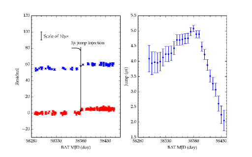
Figure 1: Left panel: The simulated pulsar (relative)timing residual for two pulsars. The x-axis is the barycentric TOA in Modified Julian Day (MJD) and the y-axis is units of time. The scale is drawn and labeled on the top-left corner of the figure. We injected a 5-$\mu$s clock jump at MJD 58380. Right panel: The recovered clock jump (y-axis) as a function of jump epoch (x-axis). One can see we recover the clock jump successfully, where the measured jump is $5.08\pm 0.1$ $\mu$s.

We now turn to the real data. The Yunnan Astronomical Observatory (YNAO) of the Chinese Academy of Science operates the Kunming 40-meter radio telescope (KM40m). The telescope was built in 2006 for the Chinese lunar-probe mission. It is located in the south-west of China (${\rm N}25^{\circ}01^{\prime}38^{\prime\prime}$, ${\rm E}102^{\circ}47^{\prime}45^{\prime\prime}$), approximately 15 kilometers away from the city of Kunming. The total collecting area of KM40m is 1250 m². Our timing data were collected using a room-temperature receiver (70 K system temperature), originally designed for communication purposes. The center frequency is 2.5 GHz and the bandwidth is 300 MHz.

We have been regularly timing five millisecond pulsars since 2017. The observing schedule is much more intense compared to a typical pulsar timing program (e.g. see [18]), as we observe the same set of pulsars almost daily. Part of our timing efforts aim at helping to identify the potential issues in the frequency-clock signal chain of telescope systems. Following the standard timing pipeline, we measured the TOAs using the software PSRCHIVE [19], and computed the timing residual using TEMPO2 [20, 14].

On the 25th of August 2018, the clock signal distributor was broken during an intense lightning storm. Switching to the back-up signal path led to a jump in the pulsar timing signal, as shown in Figure 2.

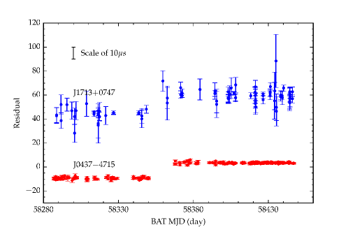
Figure 2: The timing residuals of the two most accurate millisecond pulsars in our timing array pool, i.e. PSR J1713$+$0747 and PSR J0437$-$4715. The x-axis is the barycentric TOA in Modified Julian Day (MJD) and the y-axis is the time. The scale is drawn and labeled on the top-left corner of the figure. Since the timing dataset have arbitrary offsets, we can simply compare the two pulsars in the same panel. There is a clock jitter around MJD 58355, i.e. 25/08/2018, because of the signal path switching.

The search of the clock jump is shown in Figure 3, where we compute the clock-jump value on a grid of jump epoch. The maximum clock jump value appears in the span between MJD 58350 and MJD 58365. After correcting the jump at MJD 58350, no significant clock jump can be further detected. The measured jump is $12.71\pm 0.08$ $\mu$s. We have determined the clock jump with a precision of 80 ns, which is 8 times lower than the original pulsar timing precision (600 ns for PSR 0437-4715). The 80-ns precision mainly comes from the statistical algorithm presented in this paper.

Figure 3: Upper panel: The inferred jumps as the function of jump time. The x-axis is the time in MJD, the y-axis is the amplitude of the clock jump. The inferred clock jump peaks between MJD 58350 and 58365, the amplitude is $12.71\pm 0.08$ $\mu$s. The error-bar is the standard deviation of the estimator. Note that there is a plateau from MJD 58350 to 58365. This is due to the data gap, in which time interval we can only deduce the time window of the clock jump, rather than pin down the exact epoch of clock jump. Lower panel: The inferred jumps after removing the 12.71 $\mu$s jump at MJD 58350. No jumps can be further detected with more than 1-$\sigma$ confidence.

4 Conclusion and Discussion

In this work, we have investigated a computationally efficient method to measure the observatory’s local clock jumps using pulsar timing data as the first step to build the autonomous pulsar time-scale. In order to minimize errors in determining the clock jump, we used Bayesian statistics, with which the unknown systematics can be marginalized with an analytic calculation. The estimator we adopted is the MLE, which is thought to be asymptotically optimal. We found that the Gaussian likelihood after marginalization over the noise scales leads to a distribution similar to the Student’s $t$-distribution. Using the method, we measured the clock jump at Yunnan observatory using the pulsar timing data, where 80-ns precision could be achieved using the observed data. The current precision is worse than that of widely used GPS time delivery service. Using a better receiver (e.g. 20 K noise temperature) with wider observation bandwidth (e.g. 900MHz) will bring the precision down to an 8-ns level, which will be better than that of the current GPS time delivery service. In addition, the precision can also be improved if some larger facilities can be used, for example, the Five-hundred-meter Aperture Spherical radio Telescope (FAST). FAST has just complete its initial commissioning [21] and first studies on pulsars have also been made by using it [22, 23, 24, 25, 26]. Moreover, in general, the clock precision scales as $\sim N_{\rm psr}^{1/2}$, with $N_{\rm psr}$ the number of pulsar observed. If more telescope time is available, we can time more pulsars, which would allow substantial improvement on the precision of pulsar time-scales. In this way, pulsar timing may be used as an independent method to check the local clock stability, if the GPS signal is not available or if the autonomy is the priority.

Due to the intrinsic phase confusion of the pulsar timing technique, the clock-jump value ($s$) seen in the timing residuals is the remainder of the division of the real clock jump ($s_{\rm real}$) by pulsar period $p$, i.e. $s_{\rm real}=s\,({\rm mod\,}p)$. In this way, one will not recover a clock jump that is larger than the rotational period of the pulsar in the array with the longest one. This difficultly can be resolved by observing a long period pulsar in the array. The long-period pulsar can help to derive an initial guess of the jump value. For our analysis, we used PSR B0329+54, which has a rotational period of 0.7 s. The MSP timing data can be preconditioned to the coherent state, and the final clock jump without phase confusion can be measured with the MSP ensemble.

The measured clock jump in the timing residuals refers to the barycentric dynamical time. However, in practice we need the clock jump with respect to the local terrestrial time (most of the times, Coordinated Universal Time). In this paper, we perform the reference frame correction using an iterative approach, where we can measure the clock jump in the barycentric frame, correct the local TOA with the measured jump, reform the timing residual (with timing-parameter fitting), and repeat the iteration. Once the process converges, i.e. when no further clock correction is needed, one determines the clock jump in the terrestrial frame. The iterative method thus also enables us to fit for the pulsar timing parameters.

In the current paper, we focus on the clock jump, so the timing-parameter modeling is not explicitly shown. One can include the timing parameter modeling in the Equation 7 by replacing the central value $\mu_{i}$ with the linearised timing model [14]. Here, the iterative procedure automatically takes care of the timing parameter fitting.

Pulsar timing residuals often contain red noise, i.e. time-correlated noise. In the current paper, we consider white noise only, which reduces the computational cost significantly. There are two major reasons that legitimize our decision to take such a simplified approach. Firstly, the clock jump is highly localized in time, therefore we do not need an extended dataset to measure its value. The contribution of red noise in such a short time scale is small and usually the white noise dominates. Secondly, we have marginalized the ‘Efac’ parameters, which take care of the noise systematics.

In order to get a robust error estimation, we include the ‘EFac’ in our model. We neglected the jitter noise modeling because the radiometer noise (error bars) is much larger than the jitter level. For example, the 1-hr weighted precision of J0437$-$4715 is 600 ns at YN40m, which is 6-20 times larger than the jitter noise measured [27]. Similarly, the current accuracy for the clock jump is 80 ns based on 150-day observation. The jitter noise contribution is further averaged out by another order of magnitude with the current data processing algorithm.

This work was supported by XDB23010200, 11690024, NSFC U15311243, 2015CB857101 and funding from TianShanChuangXinTuanDui and the Max-Planck Partner Group.

References

- [1] J. G. Hartnett, and A. N. Luiten, Rev. Mod. Phys. 83, 1 (2011).
- [2] D. N. Matsakis, J. H. Taylor, and T. M. Eubanks, Astron. Astropys. 326, 924 (1997).
- [3] G. Hobbs, W. Coles, R. N. Manchester, M. J. Keith, R. M. Shannon, D. Chen, M. Bailes, N. D. R.Bhat, S. Burke-Spolaor, D. Champion, A. Chaudhary, A. Hotan, J. Khoo, J. Kocz, Y. Levin, S. Oslowski, B. Preisig, V. Ravi, J. E. Reynolds, J. Sarkissian, W. van Straten, J. P. W. Verbiest, D. Yardley, and X. P. You MNRAS 427, 2780 (2012).
- [4] A. E. Rodin, and V. A. Fedorova, Astron. Rep+. 62, 378 (2018).
- [5] B. Guinot, and G. Petit, Astron. Astropys. 248, 292 (1991).
- [6] A. E. Rodin, MNRAS 387, 1583 (2008).
- [7] R. N. Caballero, K. J. Lee, L. Lentati, G. Desvignes, D. J. Champion, J. P. W. Verbiest, G. H. Janssen, B. W. Stappers, M. Kramer, P. Lazarus, A. Possenti, C. Tiburzi, D. Perrodin, S. Osłowski, S. Babak, C. G. Bassa, P. Brem, M. Burgay, I. Cognard, J. R. Gair, E. Graikou, L. Guillemot, J. W. T. Hessels, R. Karuppusamy, A. Lassus, K. Liu, J. McKee, C. M. F. Mingarelli, A. Petiteau, M. B. Purver, P. A. Rosado, S. Sanidas, A. Sesana, G. Shaifullah, R. Smits, S. R. Taylor, G. Theureau, R. van Haasteren, and A. Vecchio, MNRAS 457, 4421 (2016).
- [8] E. Kaplan, and C. Hegarty, Understanding GPS: principles and applications (Artech house, Boston, USA, 2005).
- [9] Microsemi, Datasheet of SyncSystem 4380A Master Timing Reference (Microsemi Corporate Headquarters, One Enterprise, Aliso Viejo, CA 92656 USA, 2015).
- [10] P. Lazarus, R. Karuppusamy, E. Graikou, R. N. Caballero, D. J. Champion, K. J. Lee, J. P. W. Verbiest, and M. Kramer, MNRAS 458, 868 (2016).
- [11] R. S. Foster, and D. C. Backer, ApJ 361, 300 (1990).
- [12] D. R. Lorimer and M. Kramer, Handbook of Pulsar Astronomy (Cambridge University Press, Cambridge, UK, 2012).
- [13] S. S. Wilks, Ann. Math. Stat. 9, 60 (1938).
- [14] G. B. Hobbs, R. T. Edwards, and R. N. Manchester, MNRAS 369, 655 (2006).
- [15] P. Gregory, Bayesian Logical Data Analysis for the Physical Sciences: A Comparative Approach with Mathematica ® Support (Cambridge University Press, Cambridge, UK, 2005).
- [16] I. S. Gradshteyn, and I. M. Ryzhik, Table of integrals, series, and products (Academic press, London, UK, 2014).
- [17] W. H. Press, S. A. Teukolsky, W. T. Vetterling, and B. P. Flannery, Numerical recipes in C, Vol. 2 (Cambridge university press, Cambridge, UK, 1982).
- [18] G. Desvignes, R. N. Caballero, L. Lentati, J. P. W. Verbiest, D. J. Champion, B. W. Stappers, G. H. Janssen, P. Lazarus, S. Osłowski, S. Babak, C. G. Bassa, P. Brem, M. Burgay, I. Cognard, J. R. Gair, E. Graikou, L. Guillemot, J. W. T. Hessels, A. Jessner, C. Jordan, R. Karuppusamy, M. Kramer, A. Lassus, K. Lazaridis, K. J. Lee, K. Liu, A. G. Lyne, J. McKee, C. M. F. Mingarelli, D. Perrodin, A. Petiteau, A. Possenti, M. B. Purver, P. A. Rosado, S. Sanidas, A. Sesana, G. Shaifullah, R. Smits, S. R. Taylor, G. Theureau, Tiburzi, R. van Haasteren, and A. Vecchio, MNRAS 458, 3341 (2016).
- [19] A. W. Hotan, W. van Straten, and R. N. Manchester, PASA 21, 302 (2004).
- [20] R. T. Edwards, G. B. Hobbs, and R. N. Manchester, MNRAS 372, 1549 (2006).
- [21] P. Jiang, Y. L. Yue, H. Q. Gan, R. Yao, H. Li, G. F. Pan, J. H. Sun, D. J. Yu, H¿ F. Liu, N. Y. Tang, L. Qian, J. G. Lu, J. Yan, B. Peng, S. X. Zhang, Q. M. Wang, Q. Li, D. Li, and FAST Collaboration, Sci. China-Phys. Mech. Astron. 62, 959502 (2019).
- [22] J. G Lu, B. Peng, K. Liu, P. Jiang, Y. L. Yue, M. Yu, Y. Z. Yu, F. F. Kou, L. Wang, and FAST Collaboration Sci. China-Phys. Mech. Astron. 62, 959503 (2019).
- [23] Y. Z. Yu, B. Peng, K. Liu, C. M. Zhang, L. Wang, F. F. Kou, J. G. Lu, M. Yu, and FAST Collaboration, Sci. China-Phys. Mech. Astron. 62, 959504 (2019).
- [24] J. G Lu, B. Peng, R. X. Xu, M. Yu, S. Dai, W. W. Zhu, Y. Z. Yu, P. Jiang, Y. L. Yue, L. Wang, and FAST Collaboration Sci. China-Phys. Mech. Astron. 62, 959505 (2019).
- [25] H. F. Wang, W. W. Zhu, P. Guo, D. Li, S. B. Feng, Q. Yin, C. C. Miao, Z. Z. Tao, Z. C. Pan, P. Wang, X. Zheng, X. D. Deng, Z. J. Liu, X. Y. Xie, X. H. Yu, S. P. You, H. Zhang, and FAST Collaboration, Sci. China-Phys. Mech. Astron. 62, 959507 (2019).
- [26] L. Qian, Z. C. Pan, D. Li, G. Hobbs, W. W. Zhu, P. Wang, Z. J. Liu, Y. L. Yue, Y. Zhu, H. F. Liu, D. J. Yu, J. H. Sun, P. Jiang, G. F. Pan, H. Li, H. Q. Gan, R. Yao, X. Y. Xie, F. Camilo, A. Cameron, L. Zhang, S. Wang, and FAST Collaboration, Sci. China-Phys. Mech. Astron. 62, 959508 (2019).
- [27] K. Liu, E.F. Keane, K.J. Lee, M. Kramer, J.M. Cordes, and M.B. Purver, MNRAS 420, 361 (2012).