Asymmetric nonsingular bounce from a dynamic scalar field

Abstract

We present a dynamical model for a time-asymmetric nonsingular bounce with a post-bounce change of the effective equation-of-state parameter. Specifically, we consider a scalar-field model with a time-reversal-noninvariant effective potential. [arXiv:1904.09961]

1 Introduction

A nonsingular bouncing cosmology can have several interesting properties which may remove the need for inflation; see the discussion of Ref. IjjasSteinhardt2018 and references therein. The crucial question, then, is what physics is responsible for such a nonsingular bounce of the cosmic scale factor.

Recently, a very simple suggestion has been put forward, namely to keep the structure of general relativity but to allow for degenerate metrics [$\det g_{\mu\nu}(x)=0$ at certain spacetime points]. In that case, it is possible to make an Ansatz for the metric which leads to a modified Friedmann equation with a nonsingular bouncing solution Klinkhamer2019 .

A follow-up paper KlinkhamerWang2019 has calculated certain cosmological observables (for the moment, only as Gedankenexperiments). That follow-up paper also presented, in its Appendix A, an explicit model for the time-asymmetric nonsingular bouncing cosmology discussed in Ref. IjjasSteinhardt2018 . This explicit model was constructed at the hydrodynamic level with a designer equation-of-state parameter $w(T)$, where $T$ is the cosmic time coordinate used for the metric (see Sec. 2.1).

The goal, here, is to obtain a dynamic realization of a time-asymmetric nonsingular bounce with a post-bounce change of the effective equation-of-state parameter: $w_{\text{eff,\,pre-bounce}}(T)=1$ for $T\leq 0$ and $w_{\text{eff,\,post-bounce}}(T)<1$ for $T>0$.

2 Model with a massive scalar

We take a scalar field $\phi(x)$ minimally coupled to Einstein gravity. The scalar has self-interactions determined by a special effective potential $V_{\text{eff}}(\phi)$, which is possibly related to a fundamental time asymmetry Klinkhamer2002 ; Klinkhamer2000 ; Klinkhamer2018 , as will be explained in Sec. 4. Specifically, we consider a homogenous scalar field $\phi$ that propagates over the spacetime manifold from Ref. Klinkhamer2019 .

In Sec. 2.1, we briefly review the metric Ansatz from Ref. Klinkhamer2019 , which applies to the case of a spatially flat universe. In Sec. 2.2, we introduce a dynamic scalar field and consider the reduced field equations from a particular model. In Sec. 2.3, we obtain the numerical solution of these reduced field equations, together with analytic results for the pre-bounce behavior of the solution and the asymptotic post-bounce behavior. Natural units with $c=1$ and $\hbar=1$ are used initially.

2.1 Metric Ansatz

With a cosmic time coordinate $T$ and co-moving spatial Cartesian coordinates $\{x^{1},\,x^{2},\,x^{3}\}$, the metric Ansatz for a spatially flat universe is given by Klinkhamer2019

$$ds^{2} \equiv g_{\mu\nu}(x)\,dx^{\mu}\,dx^{\nu}$$ (1a)

$$= -\frac{T^{2}}{b^{2}+T^{2}}\,dT^{2}+a^{2}(T)\;\delta_{kl}\,dx^{k}\,dx^{l}\,,$$

$$b > 0\,,$$ (1b)

$$T \in (-\infty,\,\infty)\,,\quad x^{k}\;\in\;(-\infty,\,\infty)\,,$$ (1c)

where $b$ corresponds to the regularization parameter. The corresponding spacetime manifold has topology $\mathbb{R}^{4}$.

Observe that the metric (1a) is degenerate: $\det\,g_{\mu\nu}=0$ at $T=0$. The corresponding spacetime slice at $T=0$ may be interpreted as a 3-dimensional “defect” of spacetime with topology $\mathbb{R}^{3}$. The parameter $b$ then corresponds to the characteristic length scale of this spacetime defect.

Assuming, for the moment, that the matter content of the cosmological model is solely given by a homogeneous perfect fluid with a relativistic-matter equation of state $P(\rho)=\rho/3$, the Einstein equation from the metric (1a) gives the following bounce solution of the scale factor Klinkhamer2019 :

$$a(T)=\left(\frac{b^{2}+T^{2}}{b^{2}+T_{0}^{2}}\right)^{1/4}\,,$$ (2)

where $a(T)$ has been normalized to unity at $T=T_{0}>0$. The solution (2) is perfectly smooth at $T=0$, as long as $b\neq 0$. The corresponding Kretschmann curvature scalar $K\equiv R^{\mu\nu\rho\sigma}\,R_{\mu\nu\rho\sigma}$ and the energy density $\rho$ are given by Klinkhamer2019

$$K(T) = \frac{3}{2}\;\frac{1}{\big{(}b^{2}+T^{2}\big{)}^{2}}\,,$$ (3a)

$$\rho(T) = \rho_{0}\;\frac{b^{2}+T_{0}^{2}}{b^{2}+T^{2}}\,,$$ (3b)

which are both finite at $T=0$ for nonvanishing $b$ and a finite value of $\rho_{0}$. Further details on this particular nonsingular-bouncing-cosmology scenario can be found in Refs. Klinkhamer2019 ; KlinkhamerWang2019 .

For the numerical calculations with a dynamic scalar field (to be introduced in Sec. 2.2), we will use the auxiliary coordinate $\tau\in(-\infty,\,-b]\,\cup\,[b,\,\infty)$ instead of $T\in\mathbb{R}$. These two coordinates are related as follows:

$$\tau(T)=\begin{cases}+\sqrt{b^{2}+T^{2}}\,,&\;\;\text{for}\;\;T\geq 0\,,\\[5.69054pt] -\sqrt{b^{2}+T^{2}}\,,&\;\;\text{for}\;\;T\leq 0\,,\end{cases}$$ (4)

where $\tau=-b$ and $\tau=b$ correspond to a single point ($T=0$) on the cosmic time axis (see Ref. Klinkhamer2019 for further discussion).

We remark that the coordinate transformation from $T$ to $\tau$ is not a diffeomorphism (an invertible $C^{\infty}$ function): the function (4) is discontinuous between $T=0^{-}$ and $T=0^{+}$, as is the (suitably defined) second derivative. This implies that the metric (1a) and the metric in terms of the $\tau$ coordinate (4) give rise to different differential structures of the respective spacetime manifolds (see Refs. Klinkhamer2019 ; KlinkhamerSorba2014 ; Guenther2017 for further details). Still, we can use the auxiliary $\tau$ coordinate (with appropriate boundary conditions at $\tau=\pm b$) to simplify the process of obtaining explicit solutions of the field equations.

2.2 Reduced field equations with a dynamic scalar field

We now consider a particular model for a dynamic scalar field $\phi(x)$ propagating over the spacetime manifold with metric (1a). For the cosmological applications considered, the scalar field is assumed to be spatially homogeneous and to depend solely on the cosmic time coordinate, which is taken to be the auxiliary coordinate $\tau$ from (4).

The dynamic equations for the functions $\phi(\tau)$ and $a(\tau)$ are the Klein–Gordon equation, the second-order Friedmann equation, and the first-order Friedmann equation,

$$\ddot{\phi}+3\,\left(\frac{\dot{a}}{a}\right)\,\dot{\phi}=-\frac{\partial\,V_{\text{eff}}}{\partial\phi}\,\,,$$ (5a)

$$\frac{\ddot{a}}{a}=-\frac{8\pi G_{N}}{3}\,\left(\dot{\phi}^{2}-V_{\text{eff}}-\frac{1}{2}\,\frac{a}{\dot{a}}\,\left[\frac{dV_{\text{eff}}}{d\tau}\,-\frac{\partial V_{\text{eff}}}{\partial\phi}\,\dot{\phi}\right]\right)\,,$$ (5b)

$$\left(\frac{\dot{a}}{a}\right)^{2}=\frac{8\pi G_{N}}{3}\,\left(\frac{1}{2}\,\dot{\phi}^{2}+V_{\text{eff}}\right)\,,$$ (5c)

$$V_{\text{eff}}=\Big{(}1-\exp\left[\widehat{\alpha}^{6}-a^{6}\right]\Big{)}^{2}\,\left(\frac{\text{sgn}\left[\dot{a}/a\right]+1}{2}\right)\frac{1}{2}\,m^{2}\,\phi^{2}\,,$$ (5d)

$$\phi(b)=\phi(-b)\,,$$ (5e)

$$a^{2}(b)=a^{2}(-b)\equiv\widehat{\alpha}^{2}\,,$$ (5f)

where the overdot stands for differentiation with respect to $\tau$ and the sign function is defined by

$$\text{sgn}(x) = \begin{cases}x/\sqrt{x^{2}}\,,&\;\;\text{for}\;\;x\neq 0\,,\\[5.69054pt] 0\,,&\;\;\text{for}\;\;x=0\,.\end{cases}$$ (6)

The boundary conditions (5e) and (5f) are supplemented with boundary conditions on the derivatives $\dot{\phi}$ and $\dot{a}$ at $\tau=\pm b$, in order to have well-defined functions $\phi(T)$ and $a(T)$ at $T=0$ (further details will be given in Sec. 2.3).

The effective potential (5d) consists of the standard quadratic term multiplied by two pre-factors with large brackets. The second pre-factor in (5d) gives a vanishing potential in the contracting pre-bounce phase and a nonvanishing potential in the expanding post-bounce phase, while the first pre-factor makes for a smooth start at $\tau=b$ of the nonvanishing potential in the post-bounce phase ($\tau>b$).

The ordinary differential equations (ODEs) from (5) are consistent, as can be checked by calculating the $\tau$ derivative of the first-order Friedmann equation (5c) and eliminating the obtained $\ddot{\phi}$ term by use of the Klein–Gordon equation (5a). The resulting equation is precisely the second-order Friedmann equation (5b) with the extra term on the right-hand side. This extra term reads, for the explicit choice (5d),

$$\frac{8\pi G_{N}}{6}\,\frac{a}{\dot{a}}\,\left[\dot{a}\;\frac{d}{da}\,\Big{(}1-\exp\left[\widehat{\alpha}^{6}-a^{6}\right]\Big{)}^{2}\right]\;\left(\frac{\text{sgn}\left[\dot{a}/a\right]+1}{2}\right)\,$$

$$\times\frac{1}{2}\,m^{2}\,\phi^{2}\,.$$ (7)

As mentioned before, further remarks on the effective potential (5d) appear in Sec. 4.

For later use, we introduce the definitions

$$\rho_{\phi} \equiv \frac{1}{2}\,\dot{\phi}^{2}+\frac{1}{2}\,m^{2}\,\phi^{2}\,,$$ (8a)

$$P_{\phi} \equiv \frac{1}{2}\,\dot{\phi}^{2}-\frac{1}{2}\,m^{2}\,\phi^{2}\,,$$ (8b)

$$w_{\phi} \equiv P_{\phi}/\rho_{\phi}\,,$$ (8c)

which are primarily relevant in the post-bounce phase. The two Friedmann equations (5b) and (5c) then become asymptotically ($\tau\gg b$):

$$\left.\frac{\ddot{a}}{a}\,\right|^{\text{(asymp.)}} \sim -\frac{8\pi G_{N}}{3}\,\left[\frac{1}{2}\,\rho_{\phi}+\frac{3}{2}\,P_{\phi}\right]\,,$$ (9a)

$$\left.\left(\frac{\dot{a}}{a}\right)^{2}\,\right|^{\text{(asymp.)}} \sim +\frac{8\pi G_{N}}{3}\;\rho_{\phi}\,,$$ (9b)

which shows that the quantities $\rho_{\phi}$ and $P_{\phi}$ from (8) can be interpreted as the energy density and the pressure of the asymptotic homogeneous $\phi$ field Mukhanov2005 .

Henceforth, we use reduced-Planckian units and take explicit values for $b$ and $m$ in these units,

$$8\pi G_{N}=c=\hbar=1\,,$$ (10a)

$$b=1/m=1\,,$$ (10b)

where $b$ and $1/m$ correspond, respectively, to the length scale entering the metric (1a) and the Compton wavelength of the $\phi$ scalar in the post-bounce phase.

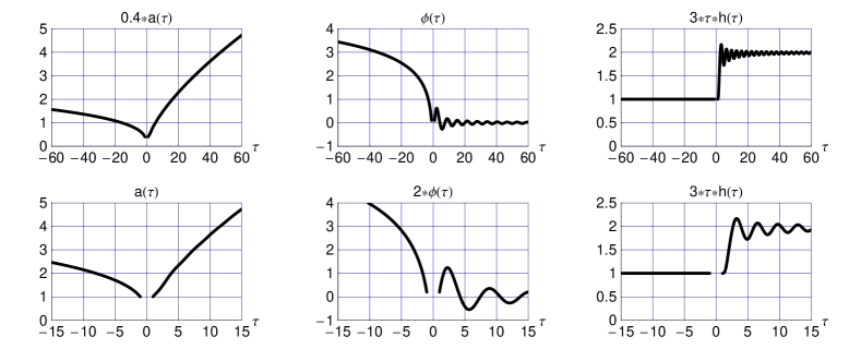
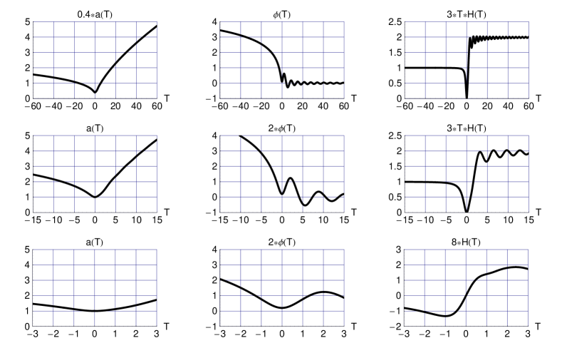
Figure 1: Numerical solution of the second-order ODEs (5a) and (5b), with boundary conditions satisfying the first-order ODE (5c) for effective potential (5d). The model parameters are $b=1/m=1$. Shown are the dynamic variables $a(\tau)$ and $\phi(\tau)$ for $|\tau|\geq b$, together with the corresponding Hubble parameter $h(\tau)\equiv[da(\tau)/d\tau]/a(\tau)$. With $b=1$, the boundary conditions are: $a(1)=a(-1)=1$, $\dot{a}(1)=-\dot{a}(-1)=1/3$, $\phi(1)=\phi(-1)=1/10$, and $\dot{\phi}(1)=-\dot{\phi}(-1)=\sqrt{2/3}\approx 0.816497$.

Figure 2: Numerical solutions $a(\tau)$ and $\phi(\tau)$ from Fig. 2 plotted with respect to $T$ as defined by (4), together with the corresponding Hubble parameter $H(T)\equiv[da(T)/dT]/a(T)$.

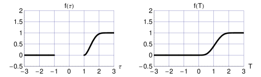
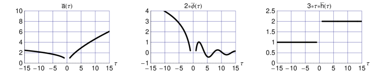
Figure 3: On the left, prefactor $f(\tau)\equiv\big{(}1-\exp\big{[}1-a^{6}(\tau)\big{]}\big{)}^{2}\,\big{(}\text{sgn}\left[h(\tau)\right]+1\big{)}\big{/}2$ entering the effective potential (5d) for the numerical solution displayed in Fig. 2 and, on the right, the corresponding prefactor $f(T)\equiv\big{(}1-\exp\big{[}1-a^{6}(T)\big{]}\big{)}^{2}\,\big{(}\text{sgn}\left[H(T)\right]+1\big{)}\big{/}2$ for the numerical solution displayed in Fig. 2.

Figure 4: Analytic expressions $\overline{a}(\tau)$, $\overline{\phi}(\tau)$, and $\overline{h}(\tau)$, as given by (11) and (13) for $b=1/m=1$ with constants $c_{1}=1/10$ and $c_{2}=\arccos\big{(}-\sqrt{3}/20\big{)}-1+\pi\approx 3.7991$.

2.3 Numerical and analytic results

We solve the ODEs (5) numerically. Specifically, we solve the two second-order equations (5a) and (5b), with boundary conditions satisfying the first-order Friedman equation (5c).

Numerical results are shown in Fig. 2 with the following boundary conditions at $\tau=\pm b$ : $a(b)=a(-b)$, $\dot{a}(b)=-\dot{a}(-b)$, $\phi(b)=\phi(-b)$, and $\dot{\phi}(b)=-\dot{\phi}(-b)$, where the $\dot{\phi}^{2}$ value at $\tau=\pm b$ follows from (5c). The top-left panel of Fig. 2, in particular, makes clear that the bounce is time-asymmetric.

Two technical remarks are in order. The first remark is that the ODEs are solved forward in cosmic time $\tau$ with the $\tau=b$ boundary conditions and backward in cosmic time $\tau$ with the $\tau=-b$ boundary conditions. The second remark is that we prefer to work with the ODEs (5a), (5b), and (5c) in terms of the auxiliary time coordinate $\tau$, rather than the corresponding ODEs in terms of the original time coordinate $T$. The reason is that the $\tau$-ODEs are nonsingular equations, whereas the $T$-ODEs are singular equations [having, for example, a term $(1+b^{2}/T^{2})\,d^{2}\phi(T)/dT^{2}$ in the Klein–Gordon equation].

As mentioned in the previous paragraph, the results of Fig. 2 are obtained with the auxiliary cosmic time coordinate $\tau$, but the physically relevant cosmic time coordinate is $T$ from (1). Using (4), the results from Fig. 2 are re-plotted with respect to $T$ in Fig. 2: the top row shows the asymptotic post-bounce behavior for $T\gg b$, the middle row the unset of oscillatory behavior of the scalar field $\phi(T)$ for $T>0$, and the bottom row the smoothness at $T=0$ (for further discussion on the smoothness, see Ref. Klinkhamer2019 and references therein).

The top-right panel in Fig. 2 has, in the asymptotic pre-bounce phase ($T\ll-b$), a Hubble parameter $H(T)\sim(1/3)\,T^{-1}$ corresponding to the scale factor $a(T)\propto(T^{2})^{1/6}$ and, in the asymptotic post-bounce phase ($T\gg b$), a Hubble parameter $H(T)\sim(2/3)\,T^{-1}$ corresponding to the scale factor $a(T)\propto T^{2/3}$. This behavior results from having effective equation-of-state parameters $w_{\text{eff,\,pre-bounce}}\sim 1$ and $w_{\text{eff,\,post-bounce}}\sim 0$. Figure 4 shows, for the obtained numerical solution, the prefactors entering the effective potential (5d).

We also have some analytic results. In the pre-bounce phase ($\tau\leq-b<0$), we obtain the following analytic solution:

$$\overline{\phi}_{\text{pre-bounce}}(\tau) = \sqrt{1/6}\,\ln(\tau^{2}/b^{2})+c_{1}\,,$$ (11a)

$$\overline{h}_{\text{pre-bounce}}(\tau) = (1/3)\,\tau^{-1}\,,$$ (11b)

$$\overline{a}_{\text{pre-bounce}}(\tau) = (\tau^{2}/b^{2})^{1/6}\,,$$ (11c)

with an appropriate constant $c_{1}$ to match the numerical value of $\phi(-1)$ from Fig. 2. Notice that if the effective potential (5d) were absent (for example, from having $m=0$), the nonsingular bouncing cosmology would be time-symmetric with the behavior (11) over the whole cosmic time axis, $\tau\in(-\infty,\,-b]\,\cup\,[b,\,\infty)$.

Moreover, it is possible to obtain analytic results for the asymptotic post-bounce behavior of the dimensionless variables $\phi(\tau)$ and $h(\tau)$. We consider $\tau\gg b$ with $V_{\text{eff}}\sim(1/2)\,m^{2}\,\phi^{2}$. Making the Ansatz

$$\phi(\tau)=\xi(\tau)\,\tau^{-1}$$ (12)

and considering the resulting $O(\tau^{-1})$ and $O(\tau^{-2})$ terms of the ODEs (5a) and (5c), we obtain the following asymptotic solution (for $\tau\gg b$):

$$\overline{\phi}_{\text{post-bounce}}(\tau)\,\Big{|}^{\text{(asymp.)}} \sim \frac{2}{\sqrt{3}}\;\frac{\cos\big{(}m\tau+c_{2}\big{)}}{m\tau}\,,$$ (13a)

$$\overline{h}_{\text{post-bounce}}(\tau)\,\Big{|}^{\text{(asymp.)}} \sim (2/3)\,\tau^{-1}\,,$$ (13b)

$$\overline{a}_{\text{post-bounce}}(\tau)\,\Big{|}^{\text{(asymp.)}} \sim (\tau/b)^{2/3}\,,$$ (13c)

with an appropriate constant $c_{2}$ to match the numerical value of $\phi(1)$ from Fig. 2. Higher-order terms are given by Eqs. (5.45) and (5.46) in Ref. Mukhanov2005 . In any case, we see that the appropriate Ansatz (12) inserted in the original ODEs (5a) and (5c) already gives the leading terms of the asymptotic solution for $\tau\gg b$.

Figure 4 shows the analytic behavior (11) and (13) over the whole $\tau$ range, even though the post-bounce results are only valid asymptotically. The analytic results from Fig. 4 may be compared with the numerical results from the bottom-row panels in Fig. 2.

Figure 5: Numerical solution of the ODEs (18a), (18), and (18), with boundary conditions satisfying (18) for effective potential (18). The model length scales are $b=1$ and $1/m=1$, and the model decay constant vanishes, $\gamma=0$. The top row shows the dynamic variables $a(\tau)$, $\phi(\tau)$, and $\rho_{\text{rel}}(\tau)$ for $|\tau|\geq b$. The middle row shows the asymptotic post-bounce behavior of certain derived quantities, the Hubble parameter $h(\tau)\equiv[da(\tau)/d\tau]/a(\tau)$ and the energy density $\rho_{\phi}(\tau)$ and pressure $P_{\phi}(\tau)$ as defined by (8). The bottom row shows the behavior near the spacetime defect at $\tau=\pm b$ with the post-bounce onset of $\phi$ oscillations (solely dampened by the expansion of the model universe). With $b=1$, the boundary conditions are: $a(1)=a(-1)=1$, $\dot{a}(1)=-\dot{a}(-1)=1/3$, $\phi(1)=\phi(-1)=1/10$, $\dot{\phi}(1)=-\dot{\phi}(-1)=\sqrt{2/3}\approx 0.816497$, and $\rho_{\text{rel}}(1)=\rho_{\text{rel}}(-1)=0$.

3 Model with a massive scalar and relativistic matter

If the massive scalar field $\phi(x)$ of Sec. 2 is coupled to other fields, then the oscillatory behavior of the post-bounce scalar field $\phi(x)$ gives rise to particle creation and reheating Kofman-etal1997 , with $w_{\text{eff}}\sim 1/3$ from massless or ultrarelativistic created particles. In this section, we present a simplified calculation for the decay of an oscillating massive scalar field propagating over the spacetime manifold with topology $\mathbb{R}^{4}$ and metric (1a). An alternative calculation for a massless scalar with quartic self-interactions is given in A.

All further calculations in this paper will be performed solely with the auxiliary coordinate $\tau$ from (4). Still, the behavior of the cosmic scale factor $a(T)$, the Hubble parameter $H(T)$, and matter fields such as $\phi(T)$ will be smooth at the defect surface $T=0$, as shown by the bottom-row panels in Fig. 2.

In Sec. 3.1, we consider the reduced field equations from a particular model that incorporates the energy exchange between the scalar field and a relativistic matter component. In Sec. 3.2, we obtain the numerical solution of these reduced field equations.

3.1 Reduced field equations

The rapid oscillations of the post-bounce scalar field $\phi$ in Fig. 2 are expected to decay rapidly Kofman-etal1997 , as long as the scalar particle $\phi$ of mass $m>0$ is coupled to light particles (for example, a scalar particle $\chi$ of mass $\mu\,m$ with $0\leq\mu\ll 1$). A coupling term $g\,m\,\phi\,\chi^{2}$ in the Lagrange density gives a tree-level decay rate $\Gamma=g^{2}\,m/(8\pi)$ for the process $\phi\to\chi\,\chi$. In a cosmological context, there are other effects which may increase the effective decay rate Mukhanov2005 , but, here, we only intend to present a simplified (but consistent) model.

Our particular model involves the bounce field $\phi(\tau)$ together with a relativistic matter component which is described by a homogeneous perfect fluid with energy density $\rho_{\text{rel}}(\tau)$ and pressure $P_{\text{rel}}(\tau)=(1/3)\,\rho_{\text{rel}}(\tau)$. In fact, the model extends the discussion of Sec. 5.5.1 in Ref. Mukhanov2005 and aims to give a consistent description of the post-bounce evolution.

Figure 6: Same as Fig. 5, but now with a nonvanishing decay constant, $\gamma=1/10$.

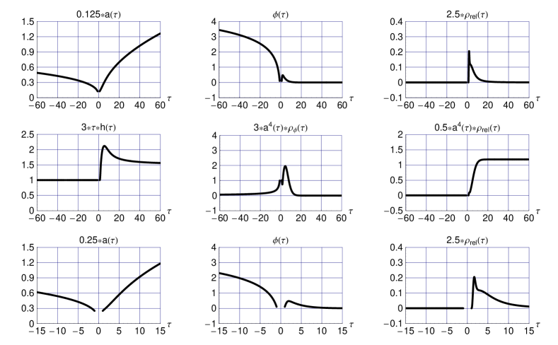
Figure 7: Same as Fig. 6, but now with a larger decay constant, $\gamma=1$.

In addition to the homogeneous scalar field $\phi(\tau)$ responsible for the bounce, we thus consider a homogeneous relativistic matter component with a constant equation-of-state parameter,

$$w_{\text{rel}}(\tau)\equiv P_{\text{rel}}(\tau)/\rho_{\text{rel}}(\tau)=1/3\,.$$ (14)

We now proceed in three steps. First, we modify the Klein–Gordon equation by the introduction of a friction term Mukhanov2005 with decay constant $\Gamma$,

$$\ddot{\phi}+3\,\big{(}\dot{a}/a+\Gamma\big{)}\,\dot{\phi}+m^{2}\,\phi=0\,,$$ (15)

where the overdot stands for differentiation with respect to $\tau$. Second, we obtain the corresponding evolution equation for $\rho_{\phi}$ from (15) and the definitions (8) for $\rho_{\phi}$ and $P_{\phi}$,

$$\dot{\rho}_{\phi}+3\,(\dot{a}/a)\,\big{(}\rho_{\phi}+P_{\phi}\big{)}=-3\,\Gamma\,\big{(}\rho_{\phi}+P_{\phi}\big{)}\,.$$ (16)

Third, energy conservation then gives the evolution equation for $\rho_{\text{rel}}$,

$$\dot{\rho}_{\text{rel}}+4\,\big{(}\dot{a}/a\big{)}\,\rho_{\text{rel}}=+3\,\Gamma\,\big{(}\rho_{\phi}+P_{\phi}\big{)}\,,$$ (17)

where the right-hand side can also be written as $3\,\Gamma\,\dot{\phi}^{2}$. The terms on the right-hand sides of (16) and (17) describe the energy exchange between the scalar-field matter component and a relativistic matter component characterized by $\rho_{\text{rel}}$ and $P_{\text{rel}}=(1/3)\,\rho_{\text{rel}}$.

Replacing the decay constant $\Gamma$ in (15) and (17) by a time-dependent quantity $\Gamma_{\text{eff}}$, the following consistent ODES are obtained:

$$\ddot{\phi}+3\,\left(\frac{\dot{a}}{a}+\Gamma_{\text{eff}}\right)\,\dot{\phi}=-\frac{\partial\,V_{\text{eff}}}{\partial\phi}\,\,,$$ (18a)

$$\dot{\rho}_{\text{rel}}+4\,\big{(}\dot{a}/a\big{)}\,\rho_{\text{rel}}=3\,\Gamma_{\text{eff}}\;\dot{\phi}^{2}\,,$$

$$\frac{\ddot{a}}{a}=-\frac{8\pi G_{N}}{3}\,\Bigg{(}\dot{\phi}^{2}-V_{\text{eff}}+\rho_{\text{rel}}-\frac{1}{2}\,\frac{a}{\dot{a}}\,\left[\frac{dV_{\text{eff}}}{d\tau}\,-\frac{\partial V_{\text{eff}}}{\partial\phi}\,\dot{\phi}\right]\Bigg{)}\,,$$

$$\left(\frac{\dot{a}}{a}\right)^{2}=\frac{8\pi G_{N}}{3}\,\left(\frac{1}{2}\,\dot{\phi}^{2}+V_{\text{eff}}+\rho_{\text{rel}}\right)\,,$$

$$V_{\text{eff}}=f\,\frac{1}{2}\,m^{2}\,\phi^{2}\,,$$

$$\Gamma_{\text{eff}}=f\,\gamma\,m\,,$$

$$f(\tau)\equiv\Big{(}1-\exp\left[\widehat{\alpha}^{6}-a^{6}(\tau)\right]\Big{)}^{2}\,\left(\frac{\text{sgn}\left[\dot{a}(\tau)/a(\tau)\right]+1}{2}\right)\,,$$

$$\phi(b)=\phi(-b)\,,$$ (18h)

$$a^{2}(b)=a^{2}(-b)\equiv\widehat{\alpha}^{2}\,,$$ (18i)

with Newton’s constant $G_{N}$ temporarily displayed and a nonnegative coupling constant $\gamma$ in $\Gamma_{\text{eff}}$ (the $\phi$-scalar mass $m$ is taken to be positive). Two technical remarks are in order. First, the additional term $\rho_{\text{rel}}$ on the right-hand side of (18) corresponds to the extra contribution $(1/2)\,\rho_{\text{rel}}+(3/2)\,P_{\text{rel}}\,$, just as in the ODE (9a) for the $\phi$ field. Second, more or less the same numerical results are obtained without the smoothing factor $\big{(}1-\exp\big{[}\widehat{\alpha}^{6}-a^{6}\big{]}\big{)}^{2}$ in $\Gamma_{\text{eff}}$ from (18) and (18).

3.2 Numerical results

We have obtained numerical solutions of the ODEs (18) for nonvanishing decay coupling constant $\gamma$ and with the same boundary conditions as in Fig. 2. For comparison, we first show in Fig. 5 (which partly reproduces Fig. 2) the numerical solution without $\phi$ decay ($\gamma=0$). The $\phi$ oscillations in the post-bounce phase give a vanishing average pressure $P_{\phi}$ and an average energy density $\rho_{\phi}\propto 1/a^{3}$, as shown by the right and mid panels of the middle row in Fig. 5. The resulting post-bounce expansion has $a(\tau)\propto\tau^{2/3}$ with Hubble parameter $h(\tau)\sim(2/3)\,\tau^{-1}$, as shown by the left panel of the middle row in Fig. 5.

With decay coupling constants $\gamma=1/10$ and $\gamma=1$, Figs. 6 and 7 show that the post-bounce $\phi$ oscillations are rapidly damped (with $\rho_{\phi}$ dropping to zero even faster than $1/a^{4}$) and that the $\phi$-oscillation energy is completely transferred to the relativistic component $\rho_{\text{rel}}\propto 1/a^{4}$. The resulting post-bounce expansion has $a(\tau)\propto\tau^{1/2}$ with Hubble parameter $h(\tau)\sim(1/2)\,\tau^{-1}$. Observe that the behavior of the post-bounce $\phi$-oscillations in the bottom-mid panels of Figs. 5–7 ranges from underdamped to overdamped.

4 Discussion

The construction of the scalar-field model for the asymmetric nonsingular bounce in Sec. 2 (and also in A) is relatively straightforward, but there is a subtle point.

Indeed, the crucial property of the effective potential $V_{\text{eff}}(\phi)$ in (5d) is its time-reversal-noninvariance: the effective potential vanishes in the contracting phase and is nonvanishing in the expanding phase. A possible origin of such an effective potential may come from a fundamental arrow-of-time, one example being the anomalous time-reversal violation Klinkhamer2002 obtained from the chiral $SO(10)$ gauge theory containing the three-family Standard Model defined over a manifold with topology $\mathbb{R}\times T^{3}$ (see Ref. Klinkhamer2000 for the original paper on the CPT anomaly and Ref. Klinkhamer2018 for a recent review).

The idea is that $V_{\text{eff}}(\phi)$ in (5d) originates from quantum effects, where the CPT anomaly Klinkhamer2002 ; Klinkhamer2000 ; Klinkhamer2018 is responsible for a microscopic “time-direction” (giving the second prefactor with the sign function in $V_{\text{eff}}$) and where gravitational effects involving $H^{2}(T)$ are responsible for the smooth turn-on (giving the first prefactor with the exponential function in $V_{\text{eff}}$). The outstanding task is to calculate such an effective potential ab initio. Note that previous results for particle creation in nonsingular bouncing cosmology appear to rely on time-reversal-noninvariant boundary conditions; see, e.g., Ref. Quintin-etal2014 .

Another issue is the physical interpretation of the fundamental scalar field $\phi(x)$ used in Secs. 2 and 3. Perhaps it is possible to interpret this fundamental scalar field $\phi(x)$ [or rather an extra copy of it] as the fluctuating component $\xi(x)$ of the composite scalar field $q(x)=q_{0}+\xi(x)$ from the so-called $q$-theory approach to the cosmological constant problem (see Refs. KV2008a ; KV2016-Lambda-cancellation ; KV2016-q-DM ; KV2016-More-on-q-DM ; KlinkhamerMistele2017 and references therein). The results of Sec. 3 then illustrate, for an assumed nonzero and positive value of $\gamma$, how the oscillating homogeneous component $\xi(x)$ of the $q$-field transfers its energy to relativistic particles in the post-bounce phase (this energy-transfer process differs from the one considered in Ref. KV2016-Lambda-cancellation ).

Appendix A Model with a massless scalar and quartic
self-interactions

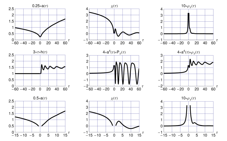
Figure 8: Numerical solution of the ODEs (5a) and (5b) with $\phi(\tau)$ replaced by $\chi(\tau)$. The boundary conditions satisfy (5c) in terms of $\chi(\tau)$, for effective potential (19). The model length scale is given by $b=1$ and the quartic coupling constant by $\lambda=1$. The top row shows the dynamic variables $a(\tau)$ and $\chi(\tau)$ for $|\tau|\geq b$, together with $\rho_{\chi}(\tau)$ from (20a). The middle row shows the asymptotic post-bounce behavior of certain derived quantities, the Hubble parameter $h(\tau)\equiv[da(\tau)/d\tau]/a(\tau)$ and the energy density $\rho_{\chi}(\tau)$ and pressure $P_{\chi}(\tau)$ as defined by (20). The bottom row shows the behavior near the spacetime defect at $\tau=\pm b$ with the post-bounce onset of $\chi$ oscillations. With $b=1$, the boundary conditions are: $a(1)=a(-1)=1$, $\dot{a}(1)=-\dot{a}(-1)=1/3$, $\chi(1)=\chi(-1)=1/10$, and $\dot{\chi}(1)=-\dot{\chi}(-1)=\sqrt{2/3}\approx 0.816497$.

Figure 9: Asymptotic post-bounce solution (26) with $\lambda=1$ and $c_{3}\approx 1.78523$. Also shown is the analytic pre-bounce solution (11) with $\overline{\phi}(\tau)$ replaced by $\overline{\chi}(\tau)$ and $\lambda=1$ and $c_{1}=1/10$.

In Sec. 2, we considered a massive free scalar $\phi$ in the post-bounce phase. Here, we take a massless scalar $\chi$ with quartic self-interactions in the post-bounce phase. The spacetime manifold has, again, topology $\mathbb{R}^{4}$ and metric (1a). The actual calculations use the auxiliary cosmic time coordinate $\tau$ from (4) and the overdot stands for differentiation with respect to $\tau$.

Specifically, we have the ODEs (5a), (5b), and (5c) with $\phi(\tau)$ replaced by $\chi(\tau)$ and the following effective potential:

$$V_{\text{eff}}=\Big{(}1-\exp\left[\widehat{\alpha}^{6}-a^{6}\right]\Big{)}^{2}\,\left(\frac{\text{sgn}\left[\dot{a}/a\right]+1}{2}\right)\,\frac{\lambda}{4}\,\chi^{4}\,,$$ (19)

with $\widehat{\alpha}^{2}\equiv a^{2}(b)=a^{2}(-b)$ and a positive coupling constant $\lambda$. Also define the following quantities:

$$\rho_{\chi} \equiv \frac{1}{2}\,\dot{\chi}^{2}+\frac{\lambda}{4}\,\chi^{4}\,,$$ (20a)

$$P_{\chi} \equiv \frac{1}{2}\,\dot{\chi}^{2}-\frac{\lambda}{4}\,\chi^{4}\,,$$ (20b)

$$w_{\chi} \equiv P_{\chi}/\rho_{\chi}\,,$$ (20c)

which are primarily relevant in the post-bounce phase. Numerical results are presented in Fig. 8. The left panel of the middle row in Fig. 8 shows that the post-bounce expansion $a\propto\tau^{1/2}$ for $\tau\gg b$ [with $h\equiv\dot{a}/a\sim(1/2)\,\tau^{-1}$] resembles the one of a standard radiation-dominated FLRW universe ($w_{\text{matter}}=1/3$), as noted already in Sec. 5.4.2. of Ref. Mukhanov2005 .

The analytic pre-bounce solution is given by (11) with $\overline{\phi}(\tau)$ replaced by $\overline{\chi}(\tau)$. We will now get the asymptotic post-bounce expressions for the dimensionless variables $\chi(\tau)$ and $h(\tau)$. Just as for the case of the quadratic potential discussed in the penultimate paragraph of Sec. 2.3, the crucial step is to make an appropriate Ansatz for $\chi(\tau)$.

Using reduced-Planckian units (10a), the relevant equations for $\chi(\tau)$ and $h(\tau)$ are

$$\ddot{\chi}+3\,h\,\dot{\chi}=-\lambda\,\chi^{3}\,,$$ (21a)

$$h^{2}=\frac{1}{3}\,\left(\frac{1}{2}\,\dot{\chi}^{2}+\frac{\lambda}{4}\,\chi^{4}\right)\,.$$ (21b)

The asymptotic solution $\chi_{\text{asymp}}(\tau)$ for $\tau\gg b>0$ will be seen to fluctuate around zero and the asymptotic solution $h_{\text{asymp}}(\tau)$ around $(1/2)\,\tau^{-1}$.

The procedure consists of two steps. First, we modify the ODE (21a) by replacing $h(\tau)$ with $(1/2)\,\tau^{-1}$ and we get

$$\left.\left(\ddot{\chi}+\frac{3}{2}\,\frac{1}{\tau}\,\dot{\chi}+\lambda\,\chi^{3}\right)\,\right|^{\text{(asymp.)}}=0\,.$$ (22)

Second, we make the following Ansatz:

$$\chi(\tau) = \eta(\rho)\;\frac{2}{\rho}\,,$$ (23a)

$$\rho(\tau) \equiv 2\,\sqrt{\tau}\,,$$ (23b)

where $\eta(\rho)$ fluctuates around zero. From (22) and (23), we obtain

$$\frac{1}{\tau^{3/2}}\,\Big{(}\eta^{\prime\prime}+\lambda\,\eta^{3}\Big{)}=0\,,$$ (24)

where the prime stands for differentiation with respect to $\rho$. As the auxiliary cosmic time coordinate $\tau$ is nonvanishing for nonzero defect scale $b$, (24) reduces to

$$\eta^{\prime\prime}+\lambda\,\eta^{3}=0\,,$$ (25)

which corresponds to a nonlinear second-order ODE (in fact, a type of Bellman’s equation, $d^{2}y/dx^{2}=k\,x^{l}\,y^{m}$ for $k=-\lambda$, $l=0$, and $m=3$).

The solution of the ODE (25) is given by a Jacobian elliptic function $\text{sn}(u\,|\,m)$, in the notation of Ref. AbramowitzStegun1965 . Taking the two integration constants appropriately (see below), the asymptotic ($\tau\gg b$) post-bounce solutions of $\chi(\tau)$ and $h(\tau)$ are given by

$$\overline{\chi}(\tau)\,\Big{|}^{\text{(asymp.)}} = \sqrt[4]{3/\lambda}\;\;\text{sn}\Big{(}\sqrt[4]{12\,\lambda}\;\sqrt{\tau}+c_{3}\,\Big{|}\,-1\Big{)}\;\;\frac{1}{\sqrt{\tau}}\,,$$

$$\overline{h}^{2}(\tau)\,\Big{|}^{\text{(asymp.)}} = \frac{1}{3}\;\left(\frac{1}{2}\,\dot{\chi}_{\text{asymp}}^{2}(\tau)+\frac{\lambda}{4}\,\chi_{\text{asymp}}^{4}(\tau)\right)\,,$$ (26b)

with a real constant $c_{3}$ that is, for the moment, set to zero. The leading behavior of $h^{2}$ from (26b), for the $\chi$ solution (26) with $c_{3}=0$, equals $(1/4)\,\tau^{-2}$ upon use of the identity $\text{cn}^{2}\,\text{dn}^{2}+\text{sn}^{4}=1$, which holds AbramowitzStegun1965 for parameter $m=-1$. The asymptotic behavior $h^{2}\sim(1/4)\,\tau^{-2}$ explains a posteriori the particular choice of one of the two integration constants needed to get (26) with $c_{3}=0$, the other integration constant is chosen to get the simplest possible argument of the sn function (an argument just proportional to $\sqrt{\tau}$). Finally, we observe from (25) that the $\rho$ variable in a particular $\eta(\rho)$ solution can be shifted by an arbitrary constant and we determine an appropriate real constant $c_{3}$ in (26) to match the numerical value of $\chi(1)$ from Fig. 8.

The asymptotic solution (26) for $\tau\gg b$ is shown in Fig. 9 and compares reasonably well with the numerical solution in Fig. 8. For completeness, the analytic pre-bounce solution for $\tau\leq-b$ is also displayed in Fig. 9. The mismatch at $\tau=\pm b$ in the left- and right-panels of Fig. 9 is of no concern, as the asymptotic solution (26) is only approximative at $\tau=b$.

References

- (1) A. Ijjas and P.J. Steinhardt, Bouncing cosmology made simple, Class. Quant. Grav. 35, 135004 (2018) [arXiv:1803.01961].
- (2) F.R. Klinkhamer, Regularized big bang singularity, Phys. Rev. D 100, 023536 (2019) [arXiv:1903.10450].
- (3) F.R. Klinkhamer and Z.L. Wang, Nonsingular bouncing cosmology from general relativity, [arXiv:1904.09961].
- (4) F.R. Klinkhamer, Fundamental time asymmetry from nontrivial space topology, Phys. Rev. D 66, 047701 (2002) [arXiv:gr-qc/0111090].
- (5) F.R. Klinkhamer, A CPT anomaly, Nucl. Phys. B 578, 277 (2000) [arXiv:hep-th/9912169].
- (6) F.R. Klinkhamer, Anomalous Lorentz and CPT violation, J. Phys. Conf. Ser. 952, 012003 (2018) [arXiv:1709.01004].
- (7) F.R. Klinkhamer and F. Sorba, Comparison of spacetime defects which are homeomorphic but not diffeomorphic, J. Math. Phys. (N.Y.) 55, 112503 (2014) [arXiv:1404.2901].
-
(8)
M. Guenther,
Skyrmion spacetime defect, degenerate metric,
and negative gravitational mass,
Master Thesis, KIT, September 2017
[available from
https://www.itp.kit.edu/en/publications/diploma]. - (9) V. Mukhanov, Physical Foundations of Cosmology (Cambridge University Press, Cambridge, England, 2005).
- (10) L. Kofman, A.D. Linde, and A.A. Starobinsky, Towards the theory of reheating after inflation, Phys. Rev. D 56, 3258 (1997) [arXiv:hep-ph/9704452].
- (11) J. Quintin, Y.F. Cai, and R.H. Brandenberger, Matter creation in a nonsingular bouncing cosmology, Phys. Rev. D 90, 063507 (2014) [arXiv:1406.6049].
- (12) F.R. Klinkhamer and G.E. Volovik, Self-tuning vacuum variable and cosmological constant, Phys. Rev. D 77, 085015 (2008) [arXiv:0711.3170].
- (13) F.R. Klinkhamer and G.E. Volovik, Dynamic cancellation of a cosmological constant and approach to the Minkowski vacuum, Mod. Phys. Lett. A 31, 1650160 (2016) [arXiv:1601.00601].
- (14) F.R. Klinkhamer and G.E. Volovik, Dark matter from dark energy in -theory, JETP Lett. 105, 74 (2017) [arXiv: 1612.02326].
- (15) F.R. Klinkhamer and G.E.Volovik, More on cold dark matter from q-theory, [arXiv:1612.04235].
- (16) F.R. Klinkhamer and T. Mistele, Classical stability of higher-derivative -theory in the four-form-field-strength realization, Int. J. Mod. Phys. A 32, 1750090 (2017) [arXiv:1704.05436].
- (17) M. Abramowitz and I.A. Stegun (editors), Handbook of Mathematical Functions (Dover Publ., New York, 1965).