(2+1)-dimensional Static Cyclic Symmetric Traversable Wormhole: Quasinormal Modes and Causality.

Abstract

In this paper we study a static cyclic symmetric traversable wormhole in $(2+1)-$dimensional gravity coupled to nonlinear electrodynamics in anti-de Sitter spacetime. The solution is characterized by three parameters: mass $M$, cosmological constant $\Lambda$ and one electromagnetic parameter, $q_{\alpha}$. The causality of this spacetime is studied, determining its maximal extension and constructing then the corresponding Kruskal-Szekeres and Penrose diagrams. The quasinormal modes (QNMs) that result from considering a massive scalar test field in the wormhole background are determined by solving in exact form the Klein-Gordon equation; the effective potential resembles the one of a harmonic oscillator shifted from its equilibrium position and, consequently, the QNMs have a pure point spectrum.

I Introduction

Anti-de Sitter gravity in $(2+1)$-dimensions has attracted a lot of attention due to its connection to a Yang-Mills theory with the Chern-Simons term Witten2007 , Achucarro1986 . Moreover, taking advantage of simplifications due to the dimensional reduction, three dimensional Einstein theory of gravity has turned out a good model from which extract relevant insights regarding the quantum nature of gravity Carlip1998 . In three spacetime dimensions, general relativity becomes a topological field theory without propagating degrees of freedom. Additionally, in string theory, there are near extremal black holes (BHs) whose entropy can be calculated and have a near-horizon geometry containing the Bañados-Teitelboim-Zanelli (BTZ) solution BTZ1992 , BTZ1993 . Particularly for the (2+1)-dimensional BTZ black hole (BH), the two-dimensional conformal description has by now well established Carlip2005 : the BTZ-BH provides a precise mathematical model of a holographic manifold. For these reasons systems where the conformal description can be carried out all the way through are very valuable.

On the other hand nonlinear electrodynamics (NLED) has gained interest for a number of reasons. Nonlinear electrodynamics consists of theories derived from Lagrangians that depend arbitrarily on the two electromagnetic invariants, $F=2(E^{2}-B^{2})$ and $G=E\cdot B$, i.e. $L(F,G)$. The ways in which $L(F,G)$ may be chosen are many, but two of them are outstanding: the Euler-Heisenberg theory Heisenberg_36 , derived from quantum electrodynamics assumptions, takes into account some nonlinear features like the interaction of light by light. And the Born-Infeld theory BI , Pleban , proposed originally with the aim of avoiding the singularity in the electric field and the self-energy due to a point charge, it is a classical effective theory that describes nonlinear features arising from the interaction of very strong electromagnetic fields, where Maxwell linear superposition principle is not valid anymore. Interesting solutions have been derived from the Einstein gravity coupled to NLED, like regular BHs, wormholes (WHs) sustained with NLED, among others, see for instance Bronnikov2017 . It is also worth to mention that some NLED arise from the spontaneous Lorentz symmetry breaking (LSB), triggered by a non-zero vacuum expectation value of the field strength Urrutia2004 .

WHs in the anti- de Sitter (AdS) gravity are interesting objects to study. For instance, regarding the transmission of information through the throat, the understanding of the details of the traversable wormhole (WH) and its quantum information implications would shed light on the lost information problem Bak2018 . The thermodynamics of a WH and its trapped surfaces was addressed in PGDiaz2009 , establishing that the accretion of phantom energy, considered as thermal radiation coming out from the WH, can significantly widen the radius of the throat. In Maldacena2004 it is shown that Euclidean geometries with two boundaries that are connected through the bulk are similar to WH in the sense that they connect two well understood asymptotic regions. In Gao2017 it is constructed a WH via a double trace deformation. Alternatively, WH solutions are constructed by gluing two spacetimes at null hypersurfaces, Kim2004 Maeda2009 . Contrasting this procedure, in a recent paper the authors derived exact solutions of the Einstein equations coupled to NLED that can be interpreted as WHs and for certain values of the parameters such solutions become the BTZ-BH Pedro2018 . Which has become an excellent laboratory for studying quantum effects since the seminal paper or94 . And regarding LSB, it can be mentioned as well that WH solutions have been derived in the context of the bumblebee gravity Ovgun1 , their QNMs have been studied in Oliveira , and the corresponding gravitational lensing in Ovgun2 .

Moreover, WHs are related to BHs; BH and WH spacetimes are obtained by identifying points in (2+1)-dimensional AdS space by means of a discrete group of isometries, some of them resulting in non-eternal BHs with collapsing WH topologies Aminneborg1998 .

In this paper we present an exact solution of the Einstein equations in (2+1)-dimensions with a negative cosmological constant (AdS) coupled to NLED. The solution can be interpreted as a WH sourced by the NLED field with a Lagrangian of the form $F^{1/2}$. This solution is a particular case of a broader family of solutions previously presented in Pedro2018 . The solution is characterized by three parameters: mass $M$, cosmological constant $-\Lambda=1/l^{2}$ and the electromagnetic parameter $q_{\alpha}$. The analogue to the Kruskal-Szekeres diagram is constructed for the WH, and the causality is investigated by means of the Penrose diagram, showing that the light trajectories traverse the WH. The WH Penrose diagram resembles the anti-de Sitter one with the WH embedded in it.

A massive scalar test field is considered in the WH background; the corresponding Klein-Gordon (KG) equation, when written in terms of the tortoise coordinate, acquires a Schrödinger-like form and it is solved in exact form determining the frequencies of the massive scalar field; the boundary conditions are of purely ingoing waves at the throat and zero outgoing waves at infinity. The effective potential in the KG equation is a confining one and, accordingly, we found that the spectrum is real, showing then that the wormhole does not swallow the field as a black hole would, but the field goes through the throat passing then to the continuation of the WH, and preserving the energy of the test field. This also shows the stability of the scalar field in this WH background.

The outline of the paper is as follows. In the next section we present the metric for the WH and the field that sources it as well as a brief review on its derivation. In Section III we find the maximal extension and then the Penrose diagram is constructed. In Section IV the KG equation for a massive scalar field is considered in the WH background. The radial sector of the KG equation, when written in terms of the tortoise coordinate, takes the form of a Schrödinger equation that is exactly solved, obtaining the QNMs by imposing the appropriate WH boundary conditions. Final remarks are given in the last section. Details on the derivation of the QNMs as well as the setting of the boundary conditions are presented as an Appendix.

II The wormhole sourced by nonlinear electrodynamics

The action of the (2+1) Einstein theory with cosmological constant, coupled to NLED is given by

$$S[g_{ab},A_{a}]=\int d^{3}x\sqrt{-g}\left(\frac{1}{16\pi}(R-2\Lambda)+L(F)\right),$$ (1)

where $R$ is the Ricci scalar and $\Lambda$ is the cosmological constant; $L(F)$ is the NLED characteristic Lagrangian. Varying this action with respect to gravitational field gives the Einstein equations,

$$G_{ab}+\Lambda g_{ab}=8\pi E_{ab},$$ (2)

where $E_{ab}$ is the electromagnetic energy-momentum tensor,

$$4\pi E_{ab}=g_{ab}L(F)-f_{ac}f_{b}{}^{c}L_{F},$$ (3)

where $L_{F}$ stands for the derivative of $L(F)$ with respect to $F$ and $f_{ab}$ are the components of the electromagnetic field tensor. The variation with respect to the electromagnetic potential $A_{a}$ entering in $f_{ab}=2\partial_{[a}A_{b]}$, yields the electromagnetic field equations,

$$\nabla_{a}(L_{F}f^{ab})=0=\nabla_{a}(_{\ast}\bm{f})^{a},$$ (4)

where $(_{\ast}\bm{f})^{a}$ is the dual electromagnetic field tensor which, for (2+1)-dimensional gravity, in terms of $f^{ab}$, is defined by $(_{\ast}\bm{f})_{a}=\frac{\sqrt{-g}}{3}\left(f^{tr}\delta^{\phi}_{a}+f^{r\phi}\delta^{t}_{a}+f^{\phi t}\delta^{r}_{a}\right)$ with $(a=t,r,\phi).$ We shall consider the particular nonlinear Lagrangian, $L(F)=\sqrt{-sF};$ these kind of Lagrangians have been called Einstein-power-Maxwell theories Hassaine2008 , Gurtug2012 . On the other hand, in Pedro2018 was shown that in $(2+1)$ Einstein theory coupled to NLED the most general form of the electromagnetic fields for stationary cyclic symmetric $(2+1)$ spacetimes, i.e., the general solution to Eqs. (4), is given by ${}_{\ast}\bm{f}=(g_{rr}c/\sqrt{-g})dr+(a/3L_{F})dt+(b/3L_{F})d\phi$, where $a$, $b$ and $c$ are constant, that by virtue of the Ricci circularity conditions, are subjected to the restriction that $ac=0=bc$. Therefore, in this geometry, in order to describe the electromagnetic field tensor, we have two disjoint branches; [$a=0=b$, $c\neq 0$] and [($a\neq 0\lor b\neq 0$), $c=0$]. Here we are considering the branch $c\neq 0$, and thus the only non-null electromagnetic field tensor component and the electromagnetic invariant are given, respectively, by

$$f^{\phi t}=\frac{3g_{rr}c}{(\sqrt{-g})^{2}},\quad F=\frac{1}{2}f^{\phi t}f_{\phi t}=\frac{9}{2}\frac{c^{2}}{g_{tt}g_{\phi\phi}}.$$ (5)

With these assumptions a five-parameter family of solutions with a charged rotating wormhole interpretation was previously presented in Pedro2018 . In this work we shall address in detail the (2+1)-dimensional static cyclic symmetric wormhole.

For the sake of completeness, we give a brief review on the derivation of the solution. The field equations of general relativity (with cosmological constant) coupled to NLED for a static cyclic symmetric (2+1)-dimensional spacetime with line element

$$ds^{2}=-N^{2}(r)dt^{2}+\frac{dr^{2}}{f^{2}(r)}+r^{2}d\phi^{2},$$ (6)

written in the orthonormal frame $\{$ $\theta^{(0)}=N(r)dt$, $\theta^{(1)}=\frac{dr}{f(r)}$, $\theta^{(2)}=rd\phi$ $\}$, are given by

$$G_{(0)}{}^{(0)}=8\pi E_{(0)}{}^{(0)}-\Lambda\delta_{(0)}^{(0)}\quad\Rightarrow\quad\frac{(f^{2})_{,r}}{2r}=2\left(L-2FL_{F}\right)-\Lambda,$$ (7)

$$G_{(1)}{}^{(1)}=8\pi E_{(1)}{}^{(1)}-\Lambda\delta_{(1)}^{(1)}\quad\Rightarrow\quad\frac{f^{2}N_{,r}}{rN}=2L-\Lambda,$$ (8)

$$G_{(2)}{}^{(2)}=8\pi E_{(2)}{}^{(2)}-\Lambda\delta_{(2)}^{(2)}\quad\Rightarrow\quad\frac{f(fN_{,r})_{,r}}{N}=2\left(L-2FL_{F}\right)-\Lambda,$$ (9)

where the comma denotes ordinary derivative with respect to the radial coordinate $r$.

The metric given by

$$ds^{2}=-\left(-q_{\alpha}Mr+q_{\beta}\sqrt{-M-\Lambda r^{2}}\right)^{2}dt^{2}+\frac{dr^{2}}{-M-\Lambda r^{2}}+r^{2}d\phi^{2},$$ (10)

is a solution of the Einstein-NLED field equations, with cosmological constant, with the nonlinear electromagnetic Lagrangian $L(F)=\sqrt{-sF}$, whose electromagnetic field tensor is given by (5) and with the electromagnetic parameter $c$ given by $c=\sqrt{2}M^{2}q_{\alpha}/(6\sqrt{s})$.

In order to obtain the solution (10), note that $L(F)=\sqrt{-sF}$ is such that $\left(L-2FL_{F}\right)=0$, then Eq.(7) becomes,

$$(f^{2})_{,r}=-2\Lambda r\Rightarrow f^{2}(r)=-M-\Lambda r^{2},$$ (11)

with $M$ being an integration constant. On the other hand, according to (5), for the line element (6) the invariant $F$ takes the form,

$$F=-\frac{1}{2}\left(\frac{3c}{rN}\right)^{2}.$$ (12)

If one replaces $F$ from Eq.(12) into $L(F)$ in Eq. (8), we arrive at

$$\frac{f^{2}N_{,r}}{rN}=2L-\Lambda\Rightarrow\frac{\left(-M-\Lambda r^{2}\right)N_{,r}}{rN}=2\sqrt{\frac{s}{2}\left(\frac{3c}{rN}\right)^{2}}-\Lambda\Rightarrow\left(-M-\Lambda r^{2}\right)N_{,r}+\Lambda rN=3\sqrt{2s}c.$$ (13)

Now, by substituting $c=\sqrt{2}M^{2}q_{\alpha}/(6\sqrt{s})$ into the previous equation, yields

$$\left(-M-\Lambda r^{2}\right)N_{,r}+\Lambda rN=M^{2}q_{\alpha},$$ (14)

whose general solution is

$$N(r)=-q_{\alpha}Mr+q_{\beta}\sqrt{-M-\Lambda r^{2}},$$ (15)

where $q_{\beta}$ is an integration constant. Finally, by substituting (11) and (15) into (9), one finds

$$\frac{f(fN_{,r})_{,r}}{N}=\sqrt{-M-\Lambda r^{2}}\frac{\left(q_{\alpha}M\frac{\Lambda r}{\sqrt{-M-\Lambda r^{2}}}-q_{\beta}\Lambda\right)}{-q_{\alpha}Mr+q_{\beta}\sqrt{-M-\Lambda r^{2}}}=\frac{\left(q_{\alpha}Mr-q_{\beta}\sqrt{-M-\Lambda r^{2}}\right)\Lambda}{-q_{\alpha}Mr+q_{\beta}\sqrt{-M-\Lambda r^{2}}}=-\Lambda,$$ (16)

such that Eq. (9) is trivially satisfied by the Lagrangian $L=\sqrt{-sF}$, the structural functions $f^{2}(r)$, $N^{2}(r)$ given by (11 ) and (15), and the electromagnetic field given by (5).

II.1 Wormhole properties

Let us show that the solution (10) allows a traversable wormhole interpretation.
The canonical metric for a (2+1)-dimensional static cyclic symmetric WH ThorneMorris is given by

$$ds^{2}=-e^{2\Phi(r)}dt^{2}+\frac{dr^{2}}{1-\frac{b(r)}{r}}+r^{2}d\phi^{2}.$$ (17)

By comparison with (10) we see that $e^{\Phi(r)}=-q_{\alpha}Mr+q_{\beta}\sqrt{-M-\Lambda r^{2}}$ and $b(r)=r(1+M+\Lambda r^{2})$, where $-\Lambda=1/l^{2}$. In this paper the case $q_{\beta}=0$ will be the subject of our study,

$$ds^{2}=-\left(-q_{\alpha}Mr\right)^{2}dt^{2}+\frac{dr^{2}}{\frac{r^{2}}{l^{2}}-M}+r^{2}d\phi^{2}\quad\textup{ with }\quad M>0.$$ (18)

Then we can check the WH properties of the metric (18):

(i) The existence of a throat $r_{0}$ where $b(r_{0})=r_{0}$. Such a throat is located at $r_{0}=\sqrt{l^{2}M}$. The range of the $r$-coordinate is in the interval $r\in[r_{0},\infty)$.

(ii) The absence of horizons. It is fulfilled since $e^{2\Phi(r)}=(-q_{\alpha}Mr)^{2}$ is nonzero for all $r\in[r_{0},\infty)$.

(iii) The fulfilment of the flaring out condition that is related to the traversability of the WH. We shall see that traversability has a consequence on the form of the QNMs. This condition is guaranteed if the derivative of $b(r)$ when evaluated at the throat is less than one, $b^{\prime}(r_{0})<1$; in our case, $b^{\prime}(r_{0})=1-2M<1$.

The nonlinear field in our case is generated by the Lagrangian $L(F)=\sqrt{-sF},$ where $F$, the electromagnetic invariant, and the only non-vanishing electromagnetic component, $f_{t\phi}$, are given, respectively, by

$$F=-\frac{M^{2}}{4sr^{4}},\quad f_{t\phi}=-\partial_{\phi}A_{t}=\frac{q_{\alpha}M^{2}}{\sqrt{2s}}.$$ (19)

Moreover, it is well known that in GR matter obeying the standard energy conditions is not worth to open a throat and so create a traversable wormhole. In the case we are analyzing, the NLED energy-momentum tensor does not satisfy the null energy condition (NEC), rendering this into a traversable WH. To check the violation of the NEC due to NLED, let us consider the null vector in the orthonormal frame, $\bm{n}=(1,1,0),$ and calculate $E_{(\alpha)(\beta)}n^{(\alpha)}n^{(\beta)}=E_{(0)(0)}+E_{(1)(1)}=L(F)/(4\pi)$, then, using (8) to determine $L(F)$, we obtain that

$$E_{(\alpha)(\beta)}n^{(\alpha)}n^{(\beta)}=-\frac{M}{8\pi r^{2}}<0,$$ (20)

from which we see that NEC is violated; particularly, evaluating at the throat $r_{0}^{2}=Ml^{2}$, $E_{(\alpha)(\beta)}n^{(\alpha)}n^{(\beta)}=-1/(8\pi l^{2})$.

III The maximal extension and causality: Kruskal-Szekeres and Penrose diagrams

In order to understand the causal structure and the structure at infinity of the WH with metric (18), we will construct its Penrose diagram. Following the standard procedure we derive first the analogue to the Kruskal-Szekeres diagram.

To start with, since the causal structure is defined by the light cones, we need to consider the radial null curves which by definition satisfy the null condition $0=ds^{2}(k^{\alpha},k^{\beta})$, $k^{\alpha}$ being a null vector; that implies

$$\frac{dt}{dr}=\pm\frac{1}{\sqrt{(r^{2}/l^{2}-M)q_{\alpha}^{2}M^{2}r^{2}}}.$$ (21)

Since the metric (18) has a coordinate singularity at $r=\sqrt{-\frac{M}{\Lambda}}=\sqrt{l^{2}M}$, we shall use the tortoise coordinate $r_{\ast}$ defined by

$$\frac{dr_{\ast}}{dr}=\sqrt{-\frac{g^{tt}}{g^{rr}}}=\frac{1}{\sqrt{({r^{2}}/{l^{2}}-M)\left(q_{\alpha}Mr\right)^{2}}}.$$ (22)

Integrating Eq. (22) for the tortoise coordinate, $r_{\ast}$, we obtain

$$r_{\ast}=-\frac{i}{2\sqrt{q_{\alpha}^{2}M^{3}}}\ln{\!\left(\frac{\sqrt{M-{r^{2}}/{l^{2}}}+\sqrt{M}}{\sqrt{M-{r^{2}}/{l^{2}}}-\sqrt{M}}\right)}.$$ (23)

We should remark that $r_{\ast}$ is real, in spite of how it looks Eq. (23). It turns out that $r_{\ast}$ in the previous form is very convenient when applying the WH boundary conditions to the KG equation. It can be shown that $r_{\ast}$ can be written equivalently as

$$r_{\ast}=-\frac{1}{\sqrt{q_{\alpha}^{2}M^{3}}}\tan^{-1}\left({\sqrt{\frac{M}{{r^{2}}/{l^{2}}-M}}}\right).$$ (24)

Since the function $\tan(x)$ is periodic, then $r_{\ast}$ is not uniquely defined in terms of $r$, i.e., for each value of $r$ there are multiple values of $r_{\ast}$, $r_{\ast}+\frac{1}{\sqrt{q_{\alpha}^{2}M^{3}}}\pi\xi_{{}_{n}}$, with $\xi_{{}_{n}}\in\mathbb{Z}$. The range of $r_{\ast}$ is determined by its values at the throat, $r_{0}$, and at infinity: at the throat $r_{\ast}(r_{0})=\frac{1}{\sqrt{q_{\alpha}^{2}M^{3}}}(-\frac{\pi}{2}+\pi\xi_{{}_{n}})$, while at the AdS infinity, $r\sim\infty$, $r_{\ast}\sim\frac{\pi\xi_{{}_{n}}}{\sqrt{q_{\alpha}^{2}M^{3}}}$, where $\xi_{{}_{n}}$ is the integer defining each particular branch. Since all these branches are equivalent, we select the branch $\xi_{{}_{n}}=1$; consequently, the range of the tortoise coordinate is $\frac{\pi}{2\sqrt{q_{\alpha}^{2}M^{3}}}\leq r_{\ast}<\frac{\pi}{\sqrt{q_{\alpha}^{2}M^{3}}}$. From Eq. (24) we can obtain $r(r_{\ast})$,

$$r^{2}=Ml^{2}\left[{1+\cot^{2}\!\left(\sqrt{q_{\alpha}^{2}M^{3}}r_{\ast}\right)}\right]=Ml^{2}\csc^{2}\!\left(\sqrt{q_{\alpha}^{2}M^{3}}r_{\ast}\right).$$ (25)

The tortoise coordinate as a function of $r$ as well as its inverse are shown in Fig. 1.

Figure 1: The tortoise coordinate $r_{\ast}$ as a function of the coordinate $r$, Eq. (24), as well as its inverse, Eq. (25) (right) are plotted; the dashed red straight lines show the position of the throat, $r_{0}^{2}=Ml^{2}$. The parameters are fixed as $M=1$, $q_{\alpha}=0.5$ and the AdS parameter is $l=2$.

In terms of the coordinates $(t,r_{\ast},\phi)$ the line element (18) becomes

$$ds^{2}=q_{\alpha}^{2}M^{2}r^{2}\left(-dt^{2}+dr^{2}_{\ast}\right)+r^{2}d\phi^{2}.$$ (26)

In terms of these coordinates the radial null geodesics satisfy $t=\pm r_{\ast}+$ constant. This motivates us to define the advanced and retarded null coordinates $v$ and $u$, respectively, by

$$v=t+r_{\ast}\quad\textup{ and }\quad u=t-r_{\ast},$$ (27)

where $-\infty<v<\infty$, $-\infty<u<\infty$. In these coordinates the metric (26) becomes

$$ds^{2}=-q_{\alpha}^{2}M^{3}l^{2}\csc^{2}{\left(\frac{u-v}{2}\sqrt{q_{\alpha}^{2}M^{3}}\right)}dudv+r^{2}d\phi^{2}.$$ (28)

From Eq. (25) and using $r_{\ast}=(v-u)/2$, it can be determined $r$ as a function of $(u,v)$ as,

$$r^{2}=l^{2}M\csc^{2}{\left(\frac{(v-u)}{2}\sqrt{q_{\alpha}^{2}M^{3}}\right)}.$$ (29)

Despite the coordinate ranges $-\infty<u<\infty$ and $-\infty<v<\infty$, the metric (28) spans only on the region $\frac{\pi}{2\sqrt{q_{\alpha}^{2}M^{3}}}\leq r_{\ast}=\frac{v-u}{2}<\frac{\pi}{\sqrt{q_{\alpha}^{2}M^{3}}}$. In order to extend the spacetime beyond the wormhole throat, $r_{0}=\sqrt{l^{2}M}$, we are going to determine the affine parameter, $\tau$, along the null geodesics and reparametrize them with the coordinates $V=V(v)$, and $U=U(u)$. We know that the geodesic tangent vector $K=K^{\beta}\partial_{\beta}=\frac{dx^{\beta}}{d\tau}\partial_{\beta}$ satisfies

$$K^{\alpha}\nabla_{\alpha}K^{\beta}=0.$$ (30)

The tangent vector can be written as $K=\frac{dr}{d\tau}\left(\pm\frac{1}{\sqrt{(r^{2}/l^{2}-M)q_{\alpha}^{2}M^{2}r^{2}}}\partial_{t}+\partial_{r}\right)$. Thus, by substituting $K^{\beta}$ into (30), we find for the affine parameter $\tau$,

$$\tau={C}_{0}\cot{\left(\frac{u-v}{2}\sqrt{q_{\alpha}^{2}M^{3}}\right)}+C_{1},$$ (31)

where ${C}_{0}$ and $C_{1}$ are integration constants. Then, the affine parameter along the null geodesics suggests to define the new coordinates $U$ and $V$ as

$$U=\cot{\left(\frac{u}{2}\sqrt{q_{\alpha}^{2}M^{3}}\right)}\quad\textup{ and }\quad V=\cot{\left(-\frac{v}{2}\sqrt{q_{\alpha}^{2}M^{3}}\right),}\quad\textup{ with ranges }\quad-\infty<U,V<\infty,$$ (32)

therefore, in terms of $U$ and $V$ the metric (28) becomes

$$ds^{2}=\frac{4l^{2}}{(U+V)^{2}}dUdV+r^{2}d\phi^{2},$$ (33)

where we have used that $r^{2}=l^{2}M(1+U^{2})(1+V^{2})/(U+V)^{2}$. By transforming to $X=(V+U)/2$ and $T=(V-U)/2$, the metric (33) can be reduced to a more usual form given by

$$ds^{2}=\frac{l^{2}}{X^{2}}\left(-dT^{2}+dX^{2}\right)+r^{2}d\phi^{2}.$$ (34)

We can see that the coordinates $(T,X)$ are the analogue to the Kruskal coordinates in Schwarzschild spacetime. In terms of $(t,r_{\ast})$ the coordinates $(T,X)$ are

$$X^{2}-T^{2}=UV=\frac{\cos\left({t\sqrt{q_{\alpha}^{2}M^{3}}}\right)+\cos\left({r_{\ast}\sqrt{q_{\alpha}^{2}M^{3}}}\right)}{\cos\left({t\sqrt{q_{\alpha}^{2}M^{3}}}\right)-\cos\left({r_{\ast}\sqrt{q_{\alpha}^{2}M^{3}}}\right)},\quad\quad\frac{X+T}{X-T}=\frac{V}{U}=\frac{\sin{\left(r_{\ast}\sqrt{q_{\alpha}^{2}M^{3}}\right)}-\sin{\left(t\sqrt{q_{\alpha}^{2}M^{3}}\right)}}{\sin{\left(r_{\ast}\sqrt{q_{\alpha}^{2}M^{3}}\right)}+\sin{\left(t\sqrt{q_{\alpha}^{2}M^{3}}\right)}}.$$ (35)

from the above equations we deduce that, in terms of $T$ and $X$, the region corresponding to the wormhole throat $r=r_{0}=\sqrt{l^{2}M}$, or $r_{\ast}=\frac{\pi}{2\sqrt{q_{\alpha}^{2}M^{3}}}$ is determined by the two equations

$$X^{2}-T^{2}=1\quad\textup{ and }\quad\frac{X+T}{X-T}=\frac{1-\sin{\left(t\sqrt{q_{\alpha}^{2}M^{3}}\right)}}{1+\sin{\left(t\sqrt{q_{\alpha}^{2}M^{3}}\right)}}$$ (36)

Since $X^{2}-T^{2}=1$, then $X\neq T$ and $\frac{X+T}{X-T}=\frac{1-\sin{\left(t\sqrt{q_{\alpha}^{2}M^{3}}\right)}}{1+\sin{\left(t\sqrt{q_{\alpha}^{2}M^{3}}\right)}}$ can be written as

$$T=m(t)X,\quad\textup{ with }\quad m(t)=-\sin(t)\in(-1,1),$$ (37)

$T=m(t)X$ corresponds to the region determined by all the straight lines that cross the origin $(X=0,T=0)$ with slope between $-1$ and $1$. The intersection between $X^{2}-T^{2}=1$ and $T=m(t)X$, yields $X^{2}-T^{2}=1$. Thus, the region corresponding to the wormhole throat in terms of $X$ and $T$, corresponds to $X^{2}-T^{2}=1$, i.e. the hyperbola with vertices at $(X=\pm 1,T=0)$.

From Eqs. (35) can be obtained that

$$T^{2}\sin^{2}{\left(r_{\ast}\sqrt{q_{\alpha}^{2}M^{3}}\right)}+X^{2}\left(\frac{T^{2}-X^{2}-1}{T^{2}-X^{2}+1}\right)^{2}\cos^{2}{\left(r_{\ast}\sqrt{q_{\alpha}^{2}M^{3}}\right)}=X^{2}.$$ (38)

Regarding infinity, from the previous equation, the asymptotic AdS region $r\sim\infty$, or $r_{\ast}\sim\frac{\pi}{\sqrt{q_{\alpha}^{2}M^{3}}}$, in terms of $X$ and $T$, is given by

$$X^{2}\left(\frac{T^{2}-X^{2}-1}{T^{2}-X^{2}+1}\right)^{2}\sim X^{2},$$ (39)

which is fulfilled by $X\sim 0$, or by the region,

$$\frac{T^{2}-X^{2}-1}{T^{2}-X^{2}+1}\sim 1\Rightarrow\left\{\quad(T^{2}-X^{2})\gg 1\quad\vee\quad(X^{2}-T^{2})\gg 1\quad\right\}$$ (41)

Collecting the regions defined by (36) and (39), the Kruskal diagram corresponding to the spacetime (18) is depicted in Fig. 2.

Figure 2: It is shown the analogue to the Kruskal-Szekeres diagram for the WH. The blue hyperbola with vertices at $(X,T)=(\pm 1,0)$, represents the WH throat. Horizontal hyperbolae with vertices at $(X,T)=(\pm\infty,0)$, as well as the region $X=0$, represent spatial infinity; the vertical hyperbola (vertices at $(X,T)=(0,\pm\infty)$) represents time infinity. In the Kruskal diagram, the hyperbola at the top (time infinity) can be identified with the one at the bottom, in case we want to work with the covering space.

In order to obtain the Penrose diagram of the spacetime in consideration, we introduce the coordinates $\lambda$ and $\rho$ given by

$$T-X=\tan{\left(\frac{\lambda-\rho}{2}\right)},\quad T+X=\tan{\left(\frac{\lambda+\rho}{2}\right)}.$$ (42)

Then, the WH metric in terms of $(\lambda,\rho)$, yields

$$ds^{2}=l^{2}\csc^{2}{\rho}\left(-d\lambda^{2}+d\rho^{2}+Md\phi^{2}\right)=\frac{l^{2}}{\sin^{2}{\rho}}\left(-d\lambda^{2}+d\rho^{2}+d\tilde{\phi}^{2}\right),\quad\textup{ with }\quad\tilde{\phi}=M\phi,$$ (43)

and where $r$ and $\rho$ are related by

$$r^{2}=l^{2}M\csc^{2}{\rho}.$$ (44)

Now in order to draw the Penrose diagram, by using (44), we can see that for the range of $\rho$, i.e., $\rho\in(-\pi,0)\cup(0,\pi)$, the regions that define the maximal extension of the spacetime correspond to

$$\textup{Wormhole throat: }\quad\left(r=r_{0}=\sqrt{l^{2}M}\right)\equiv\left(\rho=\pm\frac{\pi}{2}\right).$$ (45)

$$\textup{Asymptotic AdS regions: }\quad\left(r\sim\infty\right)\equiv\left(\rho=0,\pm\pi\right).$$ (46)

Figure 3: Penrose diagram for the WH, metric (18): Continuous vertical lines show the spatial infinity, $\rho=-\pi,0,\pi$; while the dashed ones represent WH throats, $\rho=-\pi/2,\pi/2$. The black dots at the top and at the bottom, $i^{+}$ and $i^{-}$, denote the time infinity, future and past, respectively. Every light ray coming from infinity $\rho\sim\pm\pi$ will pass through the WH throat $\rho=\pm\pi/2$, and reach infinity $\rho\sim 0$, and viceversa. In a similar way than for the BTZ Penrose diagram, the WH Penrose diagram can be embedded in the Einstein Universe.

The Penrose diagram of the spacetime with metric (18) is shown in Fig. 3. Finally, symmetries allow us to consider the Penrose diagram for the metric (18) being just half of the strip $\rho\in(-\pi,0)\cup(0,\pi)$, as shown in Fig. 4. In a similar way than the BTZ Penrose diagram, the WH Penrose diagram can be embedded into the Einstein Universe. Thus, in Fig. 4, every light ray coming from infinity $\rho\sim\pi$ will pass through the WH throat $\rho=\pi/2$, and reach infinity $\rho\sim 0$, and viceversa. According to the Penrose diagram, anything that crosses the throat is not lost, but passes to the other part of the WH, in the extended manifold.

Figure 4: Penrose diagram for the WH, metric (18): Continuous vertical lines show the spatial infinity, while the dashed one represents the WH throat. Light rays coming from infinity $\rho\sim\pi$, will pass through the WH throat $\rho=\pi/2$, and then travel towards infinity $\rho\sim 0$.

IV QNMs of a massive scalar test field in the WH spacetime

The QNMs encode the information on how a perturbing field behaves in certain spacetime; they depend on the type of perturbation and on the geometry of the background system. The QNMs of the BTZ-BH have been determined for a number of perturbing fields, namely, scalar, massive scalar, electromagnetic, etc Cardoso2001 , Birmingham2001 , Fernando2004 . In this section we address the perturbation of the previously introduced WH, (18), by a massive scalar field $\Psi(t,\vec{r})$. The effect is described by the solutions of the KG equation,

$$(\nabla^{\alpha}\nabla_{\alpha}-\mu^{2})\Psi(t,\vec{r})=0,$$ (47)

where $\mu$ is the mass of the scalar field; equivalently, the KG equation is,

$$\partial_{\alpha}\left(\sqrt{-g}g^{\alpha\beta}\partial_{\beta}\Psi(t,\vec{r})\right)-\sqrt{-g}\mu^{2}\Psi(t,\vec{r})=0.$$ (48)

The scalar field is suggested of the form

$$\Psi(t,\vec{r})=e^{-i\omega t}e^{i\ell\phi}R(r),$$ (49)

where $\omega$ is the frequency of the perturbation and $\ell$ its azimuthal angular momentum. Substituting (49) into the KG equation, we arrive at a second order equation for $R(r)$,

$$R^{\prime\prime}+\frac{2Ml^{2}-3r^{2}}{(Ml^{2}-r^{2})r}R^{\prime}-\left(\frac{\omega^{2}-q_{\alpha}M^{2}(\ell^{2}+\mu^{2}r^{2})}{q_{\alpha}M^{2}(M-{r^{2}}/{l^{2}})r^{2}}\right)R=0.$$ (50)

$R(r)$ is completely determined once the appropriate boundary conditions are imposed. Since Eq. (50) diverges at the throat, $r_{0}^{2}=-M/\Lambda=Ml^{2}$, it is useful to put the KG equation in terms of the tortoise coordinate, $r_{\ast}$, defined in Eq. (22). For the WH, with $r_{0}$ being the throat, the boundary conditions for the QNMs consist in assuming purely ingoing waves at the throat of the WH, $r=r_{0}$, that in terms of the tortoise coordinate is $R(r)\sim e^{-i\omega r_{\ast}}$. While at infinity, $r\mapsto\infty$, the AdS boundary demands the vanishing of the solution; i.e. the boundary conditions are

$${r\sim r_{0}\Rightarrow R(r)\sim e^{-i\omega r_{\ast}},}$$ (51)

$${r\sim\infty\Rightarrow R(r)\sim 0.}$$ (52)

Let us return to the radial part of the KG Eq. (50). By transforming $R(r_{\ast})=\psi(r_{\ast})/\sqrt{r}$ (considering $r$ as a function of $r_{\ast}$), we arrive at

$$\ddot{\psi}(r_{\ast})+\left[\omega^{2}-V_{\rm eff}(r_{\ast})\right]\psi(r_{\ast})=0,$$ (53)

where $\dot{f}=df/dr_{\ast}$; while the effective potential $V_{\rm eff}$ in the Schrödinger-like equation (53), is

$$V_{\rm eff}(r)=q_{\alpha}^{2}M^{2}\left[\left(\mu^{2}+\frac{3}{4l^{2}}\right)r^{2}+\ell^{2}-\frac{M}{4}\right],\quad\textup{ for }\quad r\in[r_{0},\infty)$$ (54)

that we identify as the potential of a displaced harmonic oscillator, with frequency $\omega^{2}=q_{\alpha}^{2}M^{2}(\mu^{2}+\frac{3}{4l^{2}})$. Note that the displacement is proportional to the angular momentum of the scalar field, $\ell^{2}$. The effective potential can be written in terms of the tortoise coordinate as

$$V_{\rm eff}(r_{\ast})=q_{\alpha}^{2}M^{3}\left\{\left(\mu^{2}l^{2}+\frac{3}{4}\right)\csc^{2}\!\left(\sqrt{q_{\alpha}^{2}M^{3}}r_{\ast}\right)+\frac{\ell^{2}}{M}-\frac{1}{4}\right\},\quad\textup{ for }\quad\frac{\pi}{2\sqrt{q_{\alpha}^{2}M^{3}}}\leq r_{\ast}<\frac{\pi}{\sqrt{q_{\alpha}^{2}M^{3}}}.$$ (55)

The coordinate $\rho$, that was introduced in section III, as $r^{2}=l^{2}M\csc^{2}{\rho}$ [see Eq. (44)], in contrast to the coordinates $r$ and $r_{\ast}$, covers both sides of the WH spacetime, side I: $\rho\in(0,\pi/2]$, and side II: $\rho\in[\pi/2,\pi)$, connected by the WH throat located at $\rho=\frac{\pi}{2}$. The effective potential in terms of $\rho$ is

$$V_{\rm eff}(\rho)=q_{\alpha}^{2}M^{3}\left\{\left(\mu^{2}l^{2}+\frac{3}{4}\right)\csc^{2}\!(\rho)+\frac{\ell^{2}}{M}-\frac{1}{4}\right\},\quad\textup{ for }\quad\rho\in(0,\pi).$$ (56)

The effective potential is depicted in Fig. 5, both, as a function of $r$ and of $\rho$. It diverges at infinity, being, as a function of $r$, a confining harmonic oscillator-type potential; while as a function of $\rho$ it is a potential of the Rosen-Morse type Fdez2001 .

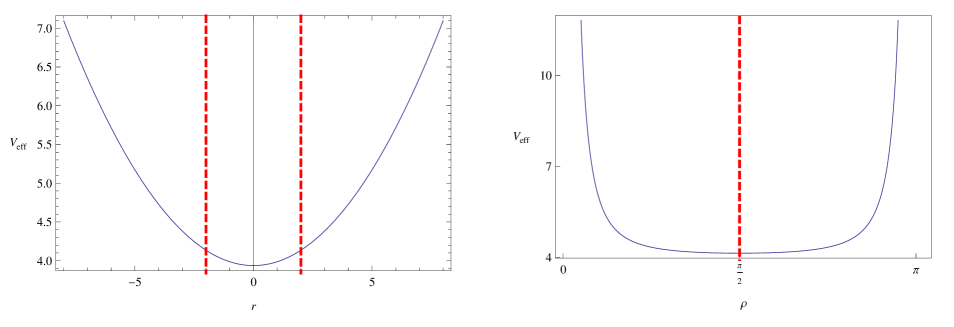
Figure 5: The effective potential as a function of the coordinate $r$ (left) and as a function of $\rho$ (right) are displayed; the dashed red vertical lines show the position of the throat, $r_{0}^{2}=Ml^{2}$ or $\rho=\pi/2$. The parameters are fixed as $M=1$, $q_{\alpha}=0.5$ and the AdS parameter is $l=2$; while the field parameters are $\ell=4,\mu=0.1$. Note that the range of the coordinate $r$ is $r_{0}\leq r<\infty$, i.e. to the right of the dashed red lines.

IV.1 The solution for the QNMs of the WH

In general, the spectrum of the Schrödinger-like operator $\hat{H}=-\frac{d^{2}}{dr^{2}_{\ast}}+V_{\rm eff}(r_{\ast})$, can be decomposed into three parts: point spectrum (often called discrete spectrum); continuous spectrum and residual spectrum. In the case of our interest it turns out that the QNMs correspond to the point spectrum and it could be foreseen from the shape of the effective potential.

In Weyl H. Weyl showed that if $V(x)$ is a real valued continuous function on the real line $\mathcal{R}=(-L,L)$, $L\in\mathbb{R}$, and such that $\lim_{|x|\rightarrow L}V(x)\rightarrow\infty$, and such that $V(x)$ is monotonic in $|x|\in(-L,L)$, then the unbounded operator $-d^{2}/dx^{2}+V(x)$, acting on $\mathbf{L}^{2}(\mathcal{R})$, has pure point spectrum. Moreover, since $V(x)$ has the structure of an infinite well, it implies that all the eigenvalues of the operator $\hat{H}=-d^{2}/dx^{2}+V(x)$ will be real numbers, necessarily. Subsequently, in Titchmarsh , this result was extended for the case in which $V(x)$ is not necessarily monotonic in $|x|\in(-L,L)$.

Specifically in our case, the potential $V_{\rm eff}(\rho)$, in Eq. (56), is a real valued continuous function in $(0,\pi)$, and since $\lim_{|\rho|\rightarrow\pi}V_{\rm eff}(\rho)=\lim_{|\rho|\rightarrow 0}V_{\rm eff}(\rho)\rightarrow\infty$, then according to Weyl ; Titchmarsh , the the Schrödinger-like operator has a pure point spectrum. Thus we can conclude that the QNMs of the scalar field in the wormhole background (18) are purely real; i.e., these QNMs are in fact normal modes (NMs) of oscillations. In agreement with the previous argument, the general solution of Eq. (53) with $V_{\rm eff}(r_{\ast})$ in Eq. (56), is given by

$$\psi(\rho)=B_{1}P^{Z}_{V}\left(\sqrt{1-\csc^{2}{\rho}}\right)+B_{2}Q^{Z}_{V}\left(\sqrt{1-\csc^{2}{\rho}}\right)=B_{1}P^{Z}_{V}\left(i\cot{\rho}\right)+B_{2}Q^{Z}_{V}\left(i\cot{\rho}\right),$$ (57)

where $B_{1}$ and $B_{2}$ are integration constants, $P^{Z}_{V}(x)$ are the associated Legendre functions of the first kind, and $Q^{Z}_{V}(x)$ are the associated Legendre functions of the second kind; while the parameters $V$ and $Z$ are given, respectively, by

$$V=\sqrt{1+\mu^{2}l^{2}}-\frac{1}{2},\quad Z=\frac{i}{\sqrt{M}}\sqrt{\ell^{2}-\frac{M}{4}-\frac{\omega^{2}}{q_{\alpha}^{2}M^{2}}}.$$ (58)

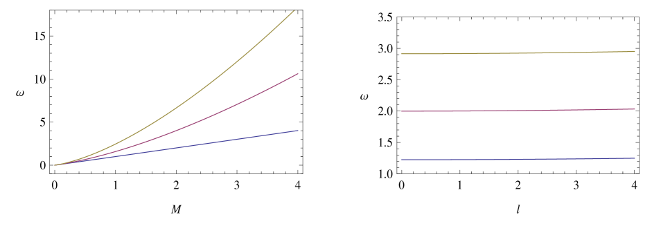
Figure 6: The quasinormal frequencies $\omega$ are shown, to the left as a function of the WH mass $M$ and to the right as a function of the AdS parameter $l$. The AdS parameter is $l=0.3$ in the plot to the left; $M=1$ in the graphic to the right. The rest of parameters are fixed as $q_{\alpha}=0.5$;$\ell=2;\mu=0.1$. The QNMs are shown for $n=0$, $n=1$ and $n=2$ in order from bottom to top.

For the sake of fluency in the text we skip the details on imposing the boundary conditions, (51) and (52), and include them in the Appendix. The boundary conditions for the QNMs consist in assuming purely ingoing waves at the throat of the WH, $r=r_{0}$, that in terms of the tortoise coordinate are $R(r)\sim e^{-i\omega r_{\ast}}$. While related to the AdS asymptotics it shall be required the vanishing of the solution at infinity, $r\mapsto\infty$; or in terms of $\rho$, $\rho\mapsto 0$ or $\rho\mapsto\pi$. These conditions imply restrictions in the values of the arguments of the Gamma functions related to the hypergeometric functions. Joining both conditions we arrive at the following restrictions for the WH parameters $(M,\Lambda,q_{\alpha})$ that combined with restrictions on the parameters of the perturbing field $(\ell,\mu,\omega)$ amount to

$$1-Z+V=-2n,\quad n\in\mathbb{N}+\{0\},$$ (59)

$$\frac{1}{2}-iM^{-3/2}\sqrt{\ell^{2}M^{2}-\frac{M^{3}}{4}-\left(\frac{\omega}{q_{\alpha}}\right)^{2}}+\sqrt{1+\mu^{2}l^{2}}=-2n,$$ (60)

$$\Rightarrow\omega^{2}=q_{\alpha}^{2}M^{3}\left[\left(2n+\frac{1}{2}+\sqrt{\mu^{2}l^{2}+1}\right)^{2}+\frac{\ell^{2}}{M}-\frac{1}{4}\right].$$ (61)

Besides, the condition (59) when applied to the solution (57) it renders that the second term becomes a multiple of the first one, and then the solution (57), in terms of the hypergeometric function, takes the form

$$\psi(\rho)=\tilde{B}_{1}\left(\frac{i\cot{\rho}+1}{i\cot{\rho}-1}\right)^{\frac{Z}{2}}\!\!\quad_{2}\!\tilde{F}_{1}\!\!\left(-V,V+1;1-Z;\frac{1-i\cot{\rho}}{2}\right),$$ (62)

being $\tilde{B}_{1}$ a constant, while ${}_{2}\!\tilde{F}_{1}\!(a,b;c;x)$ is a regularized Gauss (or ordinary) hypergeometric function, related to the Gauss hypergeometric function ${}_{2}\!F_{1}\!(a,b;c;x)$ through ${}_{2}\!\tilde{F}_{1}\!(a,b;c;x)=$ ${}_{2}\!F_{1}\!(a,b;c;x)/\Gamma(c)$, see Appendix for details.

Clearly from the expression for $\omega^{2}$, Eq. (61), we see that it is real and always positive. It may be a surprise that $\omega$ is not complex, as corresponds to an open system, as deceptively may appear a WH. However a clue that this is not the case (WH as an open system) came from the form of the effective potential. The throat is not similar to the event horizon in a BH, where amounts of fields are lost once penetrating the horizon. In the case of a WH it is supposed that the waves that penetrate the throat are passing to the continuation of the WH. This image is in agreement to the Kruskal-Szekeres and Penrose diagrams. Moreover the fact that the frequency of the QNMs has not an imaginary part, tells us that the system will remain the same, i.e. massive scalar field solutions are stable. In Fig. 6 are plotted the frequencies as a function of the mass $M$ and of the AdS parameter $l$, for $n=0,1,2$; the tendency is of growing $\omega$ as $M$ increases, we can deduce a similar behavior for the variation of the electromagnetic parameter $q_{\alpha}$, and a very slow increase of $\omega$ when $l$ increases. In here we just note that for the hypergeometric function, if the first or the second argument is a non-positive integer, then the function reduces to a polynomial. In our problem it is possible to impose that condition, by making $V=n$, being $n$ an integer; however, this is not our aim and we will not go further in this direction.

A remarkable particular case is $\ell=\pm\frac{\sqrt{M}}{2}$,

$$\pm\omega=\left(n+\frac{1}{2}\right)\omega_{0}+\left(\sqrt{\mu^{2}l^{2}+1}-\frac{1}{2}\right)\frac{\omega_{0}}{2},\textup{ with }\omega_{0}=2|q_{\alpha}|\sqrt{M^{3}}.$$ (63)

This spectrum resembles the corresponding to a quantum harmonic oscillator under the influence of an electric field $\mathcal{E}$, $E_{n}=\left(n+\frac{1}{2}\right)\hbar\omega-\frac{q^{2}\mathcal{E}^{2}}{2m\omega^{2}}$, with a frequency given by $\omega=\sqrt{\frac{k}{m}}$. i. e. for this particular frequency, $\omega_{0}=2\sqrt{M^{3}q_{\alpha}^{2}}$, the massive scalar field, confined by the WH-AdS spacetime, will oscillate harmonically.

V Final Remarks

We have determined in exact form the QNMs of a massive scalar field in the background of a charged, static, cyclic symmetric (2+1)-dimensional traversable wormhole, determining that the characteristic frequencies are real and discrete (point spectrum), showing that as far as the test scalar field is concerned, the potential is a confining one. The WH Penrose diagram agrees with this interpretation, since light trajectories passing through the WH throat arrive to the extended manifold, i.e. the other side of the WH.

Since there are no propagating degrees of freedom in the purely (2+1)-dimensional gravity, it is important to couple (2+1)-gravity with other fields as well as probe (2+1)- systems with test fields such as scalar fields. The BTZ-black hole has been of great relevance providing a mathematical model of a holographic manifold. Then (2+1)-systems in which quasinormal modes are exactly calculated, are encouraging examples for trying to go all the way through and find the correspondence with a holography theory Bertola2000 . Holographic principle, roughly speaking, consists in finding a lower-dimensional dual field theory that contains the same information as gravity. In the system worked out in the present paper, we consider two fields, an electromagnetic field, characterized by a gauge, $A^{\mu}$ that could be the starting point to try a quantization scheme. We also show that the KG equation for a massive scalar field can be exactly solvable, providing then a scalar field, that could be used in searching for a correspondence in the AdS boundary. In other words, the system worked out here stimulates to explore the possibility of obtaining the conformal field associated to this AdS-WH solution in the bulk, according to the AdS/CFT correspondence.

Acknowledgments: N. B. and P. C. acknowledges partial financial support from CONACYT-Mexico through the project No. 284489. P. C. and L. O. thank Cinvestav for hospitality.

Appendix

In this Appendix, we present the details in setting the boundary conditions for the massive scalar field in the WH spacetime with metric (18).

.1 Boundary conditions at the throat $r=r_{0}$, and at infinity $r\sim\infty$

Very close to the throat $r\sim r_{0}=\sqrt{-\frac{M}{\Lambda}}=\sqrt{l^{2}M}$ we shall require that $R(r_{\ast})\sim e^{-i\omega r_{\ast}}$. For simplicity, the description will be presented in terms of the tortoise coordinate, $r_{\ast}$. Then, the asymptotic form of $e^{-i\omega r_{\ast}}$ near the throat $r_{\ast}\sim\frac{\pi}{2\sqrt{q_{\alpha}^{2}M^{3}}}$, is given by

$$r_{\ast}\sim\frac{\pi}{2\sqrt{q_{\alpha}^{2}M^{3}}}\Rightarrow e^{-i\omega r_{\ast}}\sim\left(e^{i\pi}\right)^{-\frac{\omega}{2\sqrt{q_{\alpha}^{2}M^{3}}}}=\left(-1\right)^{-\frac{\omega}{2\sqrt{q_{\alpha}^{2}M^{3}}}}$$ (64)

In such a way that the condition (51) goes like

$$r_{\ast}\sim\frac{\pi}{2\sqrt{q_{\alpha}^{2}M^{3}}}\Rightarrow R(r_{\ast})=\frac{\psi(r_{\ast})}{r^{\frac{1}{2}}\!(r_{\ast})}\sim\left(-1\right)^{-\frac{\omega}{2\sqrt{q_{\alpha}^{2}M^{3}}}}\sim{\rm constant}\equiv\mathbb{C}-\{0\}.$$ (65)

To implement this asymptotic behavior in the solution $R(r_{\ast})=\psi(r_{\ast})/r^{\frac{1}{2}}\!(r_{\ast})$, with $\psi$ given in Eq. (57), with $\rho$ and $r_{\ast}$ related by $\rho=\sqrt{q_{\alpha}^{2}M^{3}}r_{\ast}$, recalling that the ranges are different, we shall write it as

$$R(r_{\ast})=\frac{B_{1}}{r^{\frac{1}{2}}\!(r_{\ast})}P^{Z}_{V}\!\!\left(i\cot(\sqrt{q_{\alpha}^{2}M^{3}}r_{\ast})\right)+\frac{B_{2}}{r^{\frac{1}{2}}\!(r_{\ast})}Q^{Z}_{V}\!\!\left(i\cot(\sqrt{q_{\alpha}^{2}M^{3}}r_{\ast})\right)=B_{1}R_{I}(r_{\ast})+B_{2}R_{II}(r_{\ast}),$$ (66)

the two terms, $R_{I}(r_{\ast})=\frac{1}{r^{\frac{1}{2}}\!(r_{\ast})}P^{Z}_{V}\!\!\left(i\cot(\sqrt{q_{\alpha}^{2}M^{3}}r_{\ast})\right)$ and $R_{II}(r_{\ast})=\frac{1}{r^{\frac{1}{2}}\!(r_{\ast})}Q^{Z}_{V}\!\!\left(i\cot(\sqrt{q_{\alpha}^{2}M^{3}}r_{\ast})\right)$ shall be analyzed separately. Moreover, in terms of the hypergeometric functions, the quantities $R_{I}(r_{\ast})$ and $R_{II}(r_{\ast})$ become

$$R_{I}(r_{\ast})=\frac{1}{r^{\frac{1}{2}}\!(r_{\ast})}\left(\frac{i\cot(\sqrt{q_{\alpha}^{2}M^{3}}r_{\ast})+1}{i\cot(\sqrt{q_{\alpha}^{2}M^{3}}r_{\ast})-1}\right)^{\frac{i}{2\sqrt{M}}\sqrt{\ell^{2}-\frac{M}{4}-\frac{\omega^{2}}{q_{\alpha}^{2}M^{2}}}}\!\!\!\!\!\quad_{2}\!\tilde{F}_{1}\!\!\left(-V,V+1;1-Z;\frac{1-i\cot(\sqrt{q_{\alpha}^{2}M^{3}}r_{\ast})}{2}\right),$$ (67)

The behavior of $R(r_{\ast})$ at the wormhole throat $r_{\ast}\sim\frac{\pi}{2\sqrt{q_{\alpha}^{2}M^{3}}}$ (in this neighborhood $l^{2}M-r^{2}\sim 0$) is

$$R_{I}(r_{\ast})\sim\frac{1}{\sqrt{\sqrt{l^{2}M}}}\left(\frac{i\cot(\sqrt{q_{\alpha}^{2}M^{3}}r_{\ast})+1}{i\cot(\sqrt{q_{\alpha}^{2}M^{3}}r_{\ast})-1}\right)^{\frac{i}{2\sqrt{M}}\sqrt{\ell^{2}-\frac{M}{4}-\frac{\omega^{2}}{q_{\alpha}^{2}M^{2}}}}\!\!\!\!\!\quad_{2}\!\tilde{F}_{1}\!\!\left(-V,V+1;1-Z;\frac{1}{2}\right).$$ (68)

Now, using the Bailey’s summation theorem

$$_{2}\!F_{1}\!\!\left(a,1-a;c;\frac{1}{2}\right)=\frac{\Gamma(\frac{c}{2})\Gamma(\frac{1+c}{2})}{\Gamma(\frac{c+a}{2})\Gamma(\frac{1+c-a}{2})},$$ (69)

the Eq. (68) takes the form

$$R_{I}(r_{\ast})\sim\frac{1}{\sqrt{\sqrt{l^{2}M}}}\left(\frac{i\cot(\sqrt{q_{\alpha}^{2}M^{3}}r_{\ast})+1}{i\cot(\sqrt{q_{\alpha}^{2}M^{3}}r_{\ast})-1}\right)^{\frac{i}{2\sqrt{M}}\sqrt{\ell^{2}-\frac{M}{4}-\frac{\omega^{2}}{q_{\alpha}^{2}M^{2}}}}\frac{\Gamma(\frac{1-Z}{2})\Gamma(\frac{2-Z}{2})}{\Gamma(\frac{1-V-Z}{2})\Gamma(\frac{2+V-Z}{2})}\sim R_{\ast}\frac{\Gamma(\frac{1-Z}{2})\Gamma(\frac{2-Z}{2})}{\Gamma(\frac{1-V-Z}{2})\Gamma(\frac{2+V-Z}{2})},$$ (70)

where $R_{\ast}\in\mathbb{C}-\{0\}$ is constant. While in order that $R_{I}(r_{\ast})$ behaves properly, the factor $\Gamma(\frac{1-Z}{2})\Gamma(\frac{2-Z}{2})/(\Gamma(\frac{1-V-Z}{2})\Gamma(\frac{2+V-Z}{2}))$ should be finite and non-vanishing; this can be accomplished if $\frac{1-Z}{2}$, $\frac{2-Z}{2}$, $\frac{1-V-Z}{2}$ and $\frac{2+V-Z}{2}=\frac{1}{2}+\frac{1+V-Z}{2}$, are not in the set $\{$ 0, -1, -2, -3, …. -$n$,… $\}$ with $n\in\mathbb{N};$ consequently, $1+V-Z$ $\neq$ $-1$, $-3$, $-5$, $-7$, .. $-(2n+1)$. With this restriction we get to

$$r_{\ast}\sim\frac{\pi}{2\sqrt{q_{\alpha}^{2}M^{3}}}\Rightarrow R_{I}(r_{\ast})\sim{\rm constant}\in\mathbb{C}-\{0\},$$ (71)

Having then accomplished that for $r\sim r_{0}=\sqrt{l^{2}M}\Rightarrow R_{I}(r_{\ast})\sim e^{-i\omega r_{\ast}}$ [condition (51)].

In order to get the function that describes the asymptotic behavior of the second term in $R(r_{\ast})$ as $r\sim r_{0}=\sqrt{l^{2}M}$,

$R_{II}(r_{\ast})=\frac{1}{r^{\frac{1}{2}}(r_{\ast})}Q^{Z}_{V}\!\!\left(i\cot(\sqrt{q_{\alpha}^{2}M^{3}}r_{\ast})\right)$, we write it in terms of the hypergeometric functions,

$$R_{II}(r_{\ast}) = \frac{\pi}{2}R_{I}(r_{\ast})$$

$$- \frac{\Gamma(Z+V+1)}{\Gamma(-Z+V+1)}\frac{\pi\csc{(Z\pi)}}{2r^{\frac{1}{2}}\!(r_{\ast})}\left(\frac{i\cot(\sqrt{q_{\alpha}^{2}M^{3}}r_{\ast})-1}{i\cot(\sqrt{q_{\alpha}^{2}M^{3}}r_{\ast})+1}\right)^{\!\frac{i}{2\sqrt{M}}\sqrt{\ell^{2}-\frac{M}{4}-\frac{\omega^{2}}{q_{\alpha}^{2}M^{2}}}}\!\!\!\!\!\!\!\quad_{2}\!\tilde{F}_{1}\!\!\left(-V,V+1;1+Z;\frac{1-i\cot(\sqrt{q_{\alpha}^{2}M^{3}}r_{\ast})}{2}\right).$$

Now we can analyze the behavior of $R_{II}$ as $r_{\ast}\sim\frac{\pi}{2\sqrt{q_{\alpha}^{2}M^{3}}}$,

$$R_{II}(r_{\ast}) \sim \frac{\pi}{2}R_{I}(r_{\ast})-\frac{\Gamma(Z+V+1)}{\Gamma(-Z+V+1)}\frac{\pi\csc{(Z\pi)}}{2\sqrt{\sqrt{l^{2}M}}}\left(\frac{i\cot(\sqrt{q_{\alpha}^{2}M^{3}}r_{\ast})-1}{i\cot(\sqrt{q_{\alpha}^{2}M^{3}}r_{\ast})+1}\right)^{\frac{i}{2\sqrt{M}}\sqrt{\ell^{2}-\frac{M}{4}-\frac{\omega^{2}}{q_{\alpha}^{2}M^{2}}}}\!\!\!\!\!\quad_{2}\!\tilde{F}_{1}\!\!\left(-V,V+1;1+Z;\frac{1}{2}\right),$$ (73)

$$\sim \frac{\pi}{2}R_{I}(r_{\ast})-\frac{\Gamma(Z+V+1)}{\Gamma(-Z+V+1)}\frac{\pi\csc{(Z\pi)}}{2\sqrt{\sqrt{l^{2}M}}}\left(\frac{i\cot(\sqrt{q_{\alpha}^{2}M^{3}}r_{\ast})-1}{i\cot(\sqrt{q_{\alpha}^{2}M^{3}}r_{\ast})+1}\right)^{\frac{i}{2\sqrt{M}}\sqrt{\ell^{2}-\frac{M}{4}-\frac{\omega^{2}}{q_{\alpha}^{2}M^{2}}}}\frac{\Gamma(\frac{1+Z}{2})\Gamma(\frac{2+Z}{2})}{\Gamma(\frac{1-V+Z}{2})\Gamma(\frac{2+V+Z}{2})}$$

$$\sim \frac{\pi}{2}R_{I}(r_{\ast})-\frac{\Gamma(Z+V+1)}{\Gamma(-Z+V+1)}\frac{\pi\csc{(Z\pi)}}{2\sqrt{\sqrt{l^{2}M}}}(-1)^{\frac{i}{2\sqrt{M}}\sqrt{\ell^{2}-\frac{M}{4}-\frac{\omega^{2}}{q_{\alpha}^{2}M^{2}}}}\frac{\Gamma(\frac{1+Z}{2})\Gamma(\frac{2+Z}{2})}{\Gamma(\frac{1-V+Z}{2})\Gamma(\frac{2+V+Z}{2})}.$$ (74)

Therefore we have determined the asymptotic behavior of $R_{II}(r_{\ast})$ at the throat. We considered that as $r_{\ast}\sim\frac{\pi}{2\sqrt{q_{\alpha}^{2}M^{3}}}$ i.e., ($r\sim r_{0}$), then $l^{2}M-r^{2}\sim 0$, and we also used Eq. (69).

.2 Boundary condition at infinity, $(r\sim\infty)$.

In what follows we shall impose the second boundary condition at infinity, $r\sim\infty$; in terms of the tortoise coordinate is equivalent to $r_{\ast}\sim\frac{\pi}{\sqrt{q_{\alpha}^{2}M^{3}}}$, then $R(r_{\ast})\rightarrow 0$ [condition 52]. It will be done separately for $R_{I}(r_{\ast})$ and $R_{II}(r_{\ast})$.

It shall be considered first the term $R_{I}(r_{\ast})$ written in terms of the hypergeometric function, Eq. (67). Since the last argument $x=(1-i\cot(\sqrt{q_{\alpha}^{2}M^{3}}r_{\ast}))/2$ of the hypergeometric function diverges when $r_{\ast}\sim\frac{\pi}{\sqrt{q_{\alpha}^{2}M^{3}}}$ the following identity can be used,

$${}_{2}\!F_{1}\!\!\left(a,b;c;x\right) = \Gamma(c)\!\!\!\!\!\quad_{2}\!\tilde{F}_{1}\!\!\left(a,b;c;x\right)=\frac{\Gamma(c)\Gamma(b-a)}{\Gamma(b)\Gamma(c-a)}(-x)^{-a}\!\!\!\!\!\quad_{2}\!F_{1}\!\!\left(a,a-c+1;a-b+1;\frac{1}{x}\right)$$ (75)

$$+ \frac{\Gamma(c)\Gamma(a-b)}{\Gamma(a)\Gamma(c-b)}(-x)^{-b}\!\!\!\!\!\quad_{2}\!F_{1}\!\!\left(b,b-c+1;b-a+1;\frac{1}{x}\right),$$

that allows us to write the asymptotic expression for $R_{I}(r_{\ast})$ as

$$R_{I}(r_{\ast}) \sim \frac{\Gamma(2V+1)C_{1}}{\Gamma(V+1)\Gamma(1-Z+V)}r^{V-\frac{1}{2}}(r_{\ast})\!\!\!\!\!\quad_{2}\!\tilde{F}_{1}\!\!\left(-V,Z-V;-2V;0\right)$$ (76)

$$+\!\!\!\quad\frac{\Gamma(-2V-1)C_{2}}{\Gamma(-V)\Gamma(-Z-V)}r^{-V-\frac{3}{2}}\!(r_{\ast})\!\!\!\!\!\quad_{2}\!\tilde{F}_{1}\!\!\left(V+1,Z+V+1;2V+2;0\right),$$

where $C_{1}$ and $C_{2}$ are complex constants. Using now that ${}_{2}\!F_{1}\!\!\left(a,b;c;0\right)=\Gamma(c)\!\!\!\!\!\quad_{2}\!\tilde{F}_{1}\!\!\left(a,b;c;0\right)=1/\Gamma(c)$, the previous equation can be written as

$$R_{I}(r_{\ast})\sim\frac{\Gamma(2V+1)C_{1}}{\Gamma(V+1)\Gamma(1-Z+V)}\frac{1}{\Gamma^{2}(-2V)}r^{V-\frac{1}{2}}(r_{\ast})+\!\!\!\quad\frac{\Gamma(-2V-1)C_{2}}{\Gamma(-V)\Gamma(-Z-V)}\frac{1}{\Gamma^{2}(2V+2)}r^{-V-\frac{3}{2}}(r_{\ast}).$$ (77)

On the other hand, given that $V=\sqrt{1+\mu^{2}l^{2}}-\frac{1}{2}$, and since $\mu$, $l$ $\in\mathbb{R}$ $\Rightarrow$ $\sqrt{1+\mu^{2}l^{2}}>1$ $\Rightarrow$ $V>\frac{1}{2}$. Then the behavior of $R_{I}(r)$ goes like

$$\lim_{r\rightarrow\infty}r^{V-\frac{1}{2}}\rightarrow\infty,\quad{\rm and}\lim_{r\rightarrow\infty}r^{-V-\frac{3}{2}}\rightarrow 0.$$ (78)

Therefore, the fulfilment of the proper behavior, $R_{I}(r)\sim 0$ when $r\rightarrow\infty$, and keeping the convergence of the second term in (77), imposes the condition that $(-2V-1)\neq 0,-1,-2,-3,...-n,...$ with $n\in\mathbb{N}$, guaranteeing then that $\Gamma(-2V-1)$ be finite. In other words, $(-2V-1)\neq 0,-1,-2,-3,...-n,...\Rightarrow(-2V)\neq 1,0,-1,-2,-3,...-n,...$, implying that $1/\Gamma(-2V)\neq 0$. Moreover, $V+1>0$ implies that $1/\Gamma(V+1)\neq 0$, but the fulfilment of the boundary condition that $R(r)$ vanishes at infinity requires that $1/\Gamma(1-Z+V)=0$; this condition imposes that $(1-Z+V)=0,-1,-2,-3,...-n,...$ with $n\in\mathbb{N}$. This guarantees the vanishing of the first term in (77), accomplishing then the desired behavior at infinity.

We still have to consider the compatibility of the previously determined values of $V$ and $Z$ with the fulfilment of the first boundary condition, that at the throat $R_{I}(r_{\ast})\sim e^{-i\omega r_{\ast}}$. Eq. (71) imposes that $(1-Z+V)\neq-1,-3,-5,-7,...-(2n+1),..$ with $n\in\mathbb{N}$. Gathering the two conditions lead us to the following

$$\left\{(1-Z+V)=-n:n\in\mathbb{N}\right\}-\left\{(1-Z+V)=-(2n+1):n\in\mathbb{N}\right\}=\left\{(1-Z+V)=0,-2,-4,-6,...-2n,..\right\},$$ (79)

i.e. $R_{I}(r_{\ast})$ has the asymptotic behaviors (51) and (52) provided

$$1-Z+V=-2n,\textup{ with }n\in\mathbb{N}+\{0\}.$$ (80)

.3 Behavior of $R_{II}(r_{\ast})$ at infinity

In Eq. (.1) was defined $R_{II}(r_{\ast})$. Substituting the previously derived condition (80) into (.1), leads to the vanishing of the second term of $R_{II}(r_{\ast})$ since $1/\Gamma(-Z+1+V)=0$. This will occur whenever (i) $Z$ is not an integer, otherwise $\csc{\!(Z\pi)}$ will diverge; and (ii) $1+Z+V\neq-n$ with $n\in\mathbb{N}+0$, otherwise $\Gamma(1+Z+V)$ diverges.

Summarizing, the fulfilment of the condition (80), along with $Z\neq\pm n$ and $1+Z+V\neq-n,\quad n\in\mathbb{N}+0$, leads to the following simplifications,

$$R_{II}(r_{\ast})=\frac{\pi}{2}R_{I}(r_{\ast})\Rightarrow R(r_{\ast})=B_{1}R_{I}(r_{\ast})+B_{2}R_{II}(r_{\ast})=\tilde{B}_{1}R_{I}(r_{\ast}),\quad\textup{ i.e., }R(r_{\ast})=\tilde{B}_{1}R_{I}(r_{\ast}),\quad\forall r_{\ast}.$$ (81)

Being then achieved the fulfilment of the two boundary conditions, at the throat and at infinity, for the solution $R(r_{\ast})$ for the QNMs of the scalar test field coming from the WH.

Bibliography

Bibliography

- (1) E. Witten, Three-Dimensional Gravity Revisited, arXiv: 0706.3359
- (2) A. Achúcarro, P. K. Townsend, A Chern-Simons action for three-dimensional anti-de Sitter supergravity theoriesPhys. Lett. B 180 (1986)
- (3) S. Carlip, Quantum Gravity in 2+1 Dimensions, Cambridge, UK, Cambridge University Press (1998).
- (4) M. Bañados, C. Teitelboim, J. Zanelli, The Black Hole in Three Dimensional Spacetime, Phys. Rev. Lett. 69, 1849 (1992); arXiv: hep-th/9204099.
- (5) M. Bañados, M. Henneaux, C. Teitelboim, J. Zanelli, Geometry of the 2+1 Black Hole, Phys. Rev. D 48 1506 (1993); arXiv: gr-qc/9302012.
- (6) S. Carlip, Conformal field theory, (2 + 1)-dimensional gravity and the BTZ black hole, Class. Quantum Grav. 22 (2005) R85-R123;
- (7) W. Heisenberg y H. Euler: Folgerungen aus der Diracschen Theorie des Positrons. Z. Phys 98 (1936) 714–732.
- (8) M. Born, L. Infeld: Foundations of the New Field Theory, Proc. Roy. Soc. A144 (1934) 425–451.
- (9) J.F. Plebański, Lectures on Nonlinear Electrodynamics. (Nordita, Copenhagen 1970).
- (10) K. A. Bronnikov, Nonlinear electrodynamics, regular black holes and wormholes, Int. J. Modern Phys. D, 27, 1841005 (2018); arXiv: gr-qc/1711.00087..
- (11) C. A. Escobar, L. F. Urrutia, The Goldstone theorem in nonlinear electrodynamics, Eur. J. Phys., 106, 31002 (2014);
- (12) D. Bak, C. Kim, S. Yi, Bulk View of Teleportation and Traversable Wormholes, J. High Energy Phys. 08 (2018) 140; arXiv: 1805.12349.
- (13) P. Martin-Moruno, P. Gonzalez-Diaz, Thermal Radiation from Lorentzian Wormholes, Phys. Rev. D 80 024007 (2009); arXiv: gr-qc/.0907.4055.
- (14) J. Maldacena, L. Maoz, Wormholes in AdS, J. High Energy Phys. 02, 053 (2004)
- (15) P. Gao, D. L. Jafferis and A. C. Wall, Traversable wormhole via a double trace deformation. J. High Energy Phys. 12 (2017) 151; arXiv: 1608.05687.
- (16) W. T. Kim, Traversable wormhole construction in (2+1)-Dimensions, Phys. Rev. D 79 024030 (2009); arXiv: gr-qc/0811.2962.
- (17) H. Maeda, Simple analytic model of wormhole formation, Phys. Rev. D 79 024030 (2009); arXiv: gr-qc/0811.2962.
- (18) P. Cañate, N. Breton, Black Hole-Wormhole transition in (2+1) Einstein -anti- de Sitter Gravity Coupled to Nonlinear Electrodynamics, Phys. Rev. D 98 104012 (2018); arXiv: gr-qc/1810.12111
- (19) V. Lifschytz and M. Ortiz, Scalar field quantization on the (2+1)-dimensional black hole background, Phys. Rev. D 49 1929 (1994); arXiv: gr-qc/9310008
- (20) A. Övgün, K. Jusufi, İ. Sakalli, Thermal Radiation from Lorentzian WormholesExact traversable wormhole solution in bumblebee gravity, Phys. Rev. D 99 024042 (2019); arXiv: 1804.09911.
- (21) R. Oliveira, D. M. Pantos, V. Santos, C. A. S. Almeida, Quasinormal modes of Bumblebee Wormholes, Phys. Rev. D 80 024007 (2009); arXiv:1812.01798.
- (22) A. Övgün, K. Jusufi, İ. Sakalli, Gravitational lensing under the effect of Weyl and Bumblebee Gravities, Ann. of Phys. 399 193 (2018); arXiv:1805.09431
- (23) S. Aminneborg et al, Black holes and wormholes in (2+1)-dimensions, Class. Quantum Grav. 15 627 (1998).
- (24) M. Hassaine, C. Martínez, Higher-dimensional charged black hole solutions with nonlinear electrodynamics source, Class. Quantum Grav. 25, 195023 (2008), arXiv: hep-th/0803.2946
- (25) O. Gurtug, S. H. Mzharimousavi, M. Halilsoy, 2+1-dimensional electrically charged black holes in Einstein-power-Maxwell theory, Phys. Rev. D 85, 104004 (2012); arXiv: gr-qc/1010.2340
- (26) K. Thorne, M. Morris, Wormholes in Spacetime and their use for Interstellar Travel: A Tool for Teaching General Relativity, Am. J. Phys 56, 395 (1988); M. S. Morris, K. S. Thorne and U. Yurtsever, Wormholes, Time Machines, and the Weak Energy Condition, Phys. Rev. Lett. 61, 1446 (1988);
- (27) V. Cardoso, J. P. Lemos, Scalar, electromagnetic and Weyl perturbations of BTZ black holes: Quasinormal modes, Phys. Rev. D 63, 124015 (2001); arXiv: gr-qc/0101052.
- (28) D. Birmingham, Choptuik scaling and quasinormal modes in the anti-de Sitter space/conformal field theory correspondence, Phys. Rev. D 64, 064024 (2001).
- (29) S. Fernando, Quasinormal Modes of Charged Dilaton Black Hole in 2+1 Dimensons, Gen. Relativ. Gravit. 36, 71-82 (2004).
- (30) S. Dominguez-Hernandez, D. J. Fernandez, Rosen-Morse Potential and Its Supersymmetric Partners, Int. J. Theor. Phys. 501993-2001 (2011).
- (31) M. Bertola, J. Bros, U. Moschella and R. Schaeffer, A general construccion of conformal field theories from scalar anti-de Sitter quantum field theories, Nucl. Phys. B, 587, (2000) 619; arXiv: hep-th/ 9908140
- (32) H. Weyl, Über gewöhnliche Differentialgleichungen mit Singularitäten und die zugehörigen Entwicklungen willkürlicher Funktionen. Math. Ann. 68 (1910), 220-269.
- (33) E. C. Titchmarsh, Eigenfunction Expansions Associated with Second Order Differential Equations. Clarendon Press, Oxford, 1946.