Word-level Speech Recognition
with a Letter to Word Encoder

Abstract

We propose a direct-to-word sequence model which uses a word network to learn word embeddings from letters. The word network can be integrated seamlessly with arbitrary sequence models including Connectionist Temporal Classification and encoder-decoder models with attention. We show our direct-to-word model can achieve word error rate gains over sub-word level models for speech recognition. We also show that our direct-to-word approach retains the ability to predict words not seen at training time without any retraining. Finally, we demonstrate that a word-level model can use a larger stride than a sub-word level model while maintaining accuracy. This makes the model more efficient both for training and inference.

1 Introduction

Predicting words directly has the potential to allow for more accurate, more efficient and simpler end-to-end automatic speech recognition (ASR) systems. For example, outputting words enables a word-level learning objective which more directly optimizes the quality of the transcription. While phonemes last 50-150 milliseconds and graphemes can be shorter or even silent, words are on average much longer. This allows the acoustic model to capture meaning more holistically, operating at a lower frequency with a larger context. To operate at a lower frequency the acoustic model takes larger strides (e.g. sub-samples more), which contributes to a much faster transcription speed and a lower memory footprint.

One major hurdle for direct-to-word approaches is transcribing words not found in the training vocabulary. Unlike phone-based or letter-based systems, the output lexicon in a word-based model is bounded by the words observed in the training transcriptions. Here, we propose an end-to-end model which outputs words directly, yet is still able to dynamically modify the lexicon with words not seen at training time. The method consists in jointly training an acoustic model which outputs word embeddings with a sub-word model (e.g. graphemes or word pieces) which also outputs word embeddings. The transcription of a new word is generated by inputting the individual tokens of the word into the sub-word model to obtain an embedding. We then match this embedding to the output of the acoustic model. For instance, assume the word “caterpillar” was not seen at training time, but “cat” and “pillar” were. If we input “caterpillar” into the word embedding model it should yield an embedding close to the embedding of the acoustic model when observing speech with the words “cat” and “pillar”.

Another hurdle for direct-to-word approaches is the need for massive datasets since some words may be seen only a few times in a data set with even 1,000 hours of speech. For example, Soltau et al. (2016) demonstrate competitive word-based speech recognition but require 100,000 hours of captioned video to do so. Our approach circumvents this issue by learning an embedding from the sub-word tokens of the word. By jointly optimizing the word model and the acoustic model, we gain the added advantage of learning acoustically relevant word embeddings. In order to efficiently optimize both the acoustic and word models simultaneously, we use a simple sampling based approach to approximate the normalization term over the full vocabulary. We also show how to efficiently integrate the word model with a beam search decoder.

We validate our method on two commonly used models for end-to-end speech recognition. The first is a Connectionist Temporal Classification (CTC) model Graves et al. (2006) and the second is a sequence-to-sequence model with attention (seq2seq) Bahdanau et al. (2014); Cho et al. (2014); Sutskever et al. (2014). We show competitive performance with both approaches and demonstrate the advantage of predicting words directly, especially when decoding without the use of an external language model. We also validate that our method enables the use of a dynamic lexicon and can predict words not seen at training time more accurately than a word piece baseline. Finally, we show that with our word level model, we are able to surpass state-of-the-art word error rate (WER) for end-to-end models on a low resource speech recognition benchmark.

2 Related Work

Our work builds on a large body of research in end-to-end sequence models in general and also in speech recognition (Amodei et al., 2016; Bahdanau et al., 2016; Chan et al., 2016; Collobert et al., 2016). The direct-to-word approach can be used with structured loss functions including Connectionist Temporal Classification (CTC) Graves et al. (2006) and the Auto Segmentation Criterion (ASG) Collobert et al. (2016) or less structured sequence-to-sequence models with attention Bahdanau et al. (2014).

Unlike lexicon-free approaches Likhomanenko et al. (2019); Maas et al. (2015); Zeyer et al. (2018) our model requires a lexicon. However, the lexicon is adaptable allowing for a different lexicon to be used at inference than that used during training. Traditional speech recognizers also have adaptable lexicons, which they achieve by predicting phonemes and requiring a model for grapheme-to-phoneme conversion Bisani and Ney (2008); Rao et al. (2015). Direct to grapheme speech recognition Kanthak and Ney (2002); Killer et al. (2003) circumvents the need for the grapheme-to-phoneme model but suffers from other drawbacks including (1) inefficiency due to a high-frame rate and (2) optimizing the letter error rate instead of the word error rate. In contrast, we show that it is possible to predict words directly while retaining an adaptable lexicon.

Prior work has also attempted direct-to-word speech recognition Audhkhasi et al. (2017); Li et al. (2018); Soltau et al. (2016). These approaches require massive data sets to work well Soltau et al. (2016) and do not have adaptable lexicons. Similar to our work is that of Bengio and Heigold (2014), who learn to predict word embeddings by using a sub-word level embedding model. However, their model is not end-to-end in that it requires an aligned training dataset and only uses the word model for lattice re-scoring. They also use a triplet ranking loss to learn the word embeddings, whereas our word model integrates seamlessly with common loss functions such as CTC or categorical cross entropy. Building on this work, Settle et al. (2019) keep the triplet loss but update the model to an end-to-end architecture. Their lexicon was, however, limited to up to 20k words.

One benefit of the direct-to-word approach is that optimizing a word-level loss can lead to a more direct improvement in WER. Prior work has attempted to build structured loss functions which optimize a higher-level error metric. Discriminative loss functions like Minimum Bayes Risk training can be used to optimize the WER directly but are not end-to-end Gibson and Hain (2006). On the other hand, end-to-end approaches are often non-differentiable Graves and Jaitly (2014); Prabhavalkar et al. (2018), or can be quite complex and difficult to implement Collobert et al. (2019). In contrast, the word model we propose is easy to use with existing end-to-end models.

Similar approaches to building word representations from characters have been studied for tasks in language processing Bojanowski et al. (2017); Kim et al. (2016); Labeau and Allauzen (2017); Ling et al. (2015a). Santos and Zadrozny (2014) apply a convolutional model to construct word embeddings from characters. Our work differs from this work in that (1) we show how to integrate word-level embeddings with structured loss functions like CTC that are commonly used in speech recognition and (2) we use a sampling approach to efficiently compute the lexicon-level normalization term when training the model. Ling et al. (2015b) propose a hierarchical character-to-word based sequence-to-sequence model for machine translation. This approach generates new words character-by-character and hence is more computationally expensive and not easily generalizable for use with structured loss functions like CTC.

3 Model

Figure 1: A CTC trained acoustic model combined with the letter-based word model. The $\varnothing$ denotes blank.

Figure 2: A seq2seq model combined with the letter-based word model. The function $g(\cdot)$ denotes the decoder Transformer.

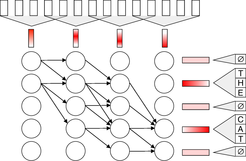
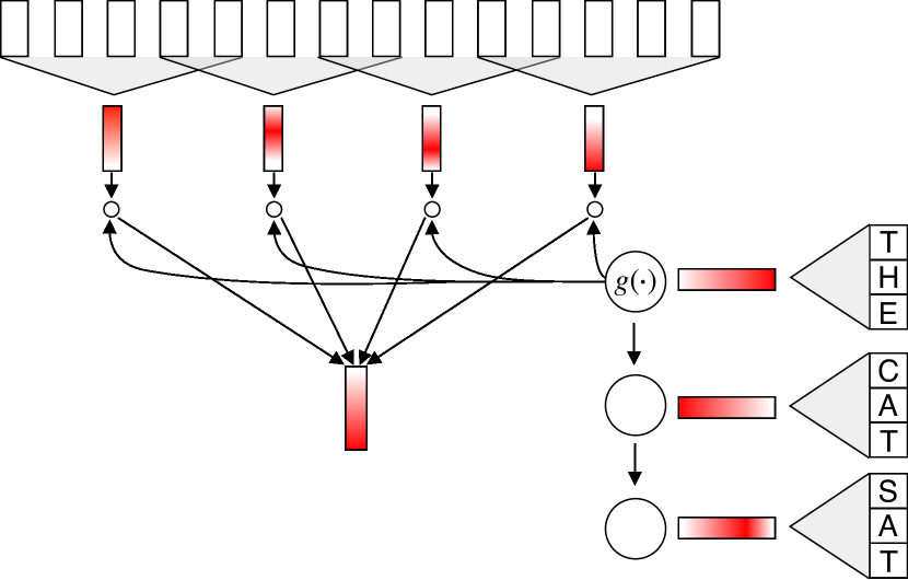
We consider a standard speech recognition setting, where we are given audio-sentence pairs $(\mathbf{X},\,\mathbf{Y})$ at training time. $\mathbf{X}=\{\mathbf{x}_{1},\,\dots,\mathbf{x}_{T}\}$ is a sequence of acoustic frames (e.g. log-mel filterbanks), and $\mathbf{Y}=\{y_{1},\,\dots y_{N}\}$ is a sequence of words with each $y_{i}$ in the lexicon ${\cal D}$. We are interested in models mapping $\mathbf{X}$ to $\mathbf{Y}$ in an end-to-end manner. We consider two approaches: (1) a structured-output learning approach, leveraging a sequence-level criterion like CTC, and (2) a sequence-to-sequence (seq2seq) approach, leveraging an encoder-decoder model with attention. Figures 2 and 2 give a high-level overview of our proposed approach combined with CTC and seq2seq models respectively.

As mentioned in Section 1, word-level end-to-end approaches face generalization issues regarding rare words, as well as challenges in addressing out-of-vocabulary words (which commonly occur at inference time in ASR). To cope with these issues, we consider an acoustic model $f^{am}(\mathbf{W}|\mathbf{X})$ which relies on word embeddings to represent any word $y\in{\cal D}$ in the lexicon by a $d$-dimensional vector $\mathbf{W}_{y}\in\mathbb{R}^{d}$. As the acoustic model relies strictly on word embeddings to represent words, the model may operate on a different lexicon ${\cal D^{\prime}}$ (say at inference), assuming one can provide corresponding word embeddings $\mathbf{W}^{\prime}$.

Word embeddings $\mathbf{W}$ are computed with a specific network architecture $f^{wd}(\cdot)$, which operates over sub-word units (in our case letters). The acoustic model $f^{am}(\cdot)$ and word model $f^{wd}(\cdot)$ are trained jointly, forcing both models to operate in the same acoustically-meaningful $d$-dimensional embedding space. In the following, we detail the word model, as well as the CTC and seq2seq combined acoustic and word model approaches.

3.1 Letter-based Word Modeling

Figure 3: Architecture of the letter to word embedding model.

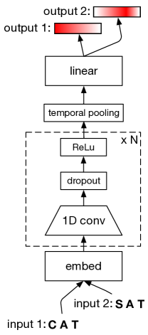
The word model $f^{wd}(\mathbf{\sigma}(y))$ maps any word $y\in{\cal D}$ into a $d$-dimensional space. As shown in Figure 3, it takes as input the sequence of letters $\mathbf{\sigma}(y)$ of the word, and performs a series of 1D-convolutions interleaved with ReLU non-linearities. For our word models, we use $N\!=\!3$ layers of convolution, the first at a stride of 1 and the second and third at a stride of 2. Each output of the last convolution depends on a fixed number ($n$) of input characters (as determined by the strides and kernel sizes) which can be seen as an $n$-gram embedding for each input. A fixed-sized embedding for the full word is obtained by a 1D max-pooling aggregation over these n-gram representations, followed by a linear layer.

One can efficiently compute the embedding of all words in the dictionary by batching several words together. When batching, an extra <pad> character is used to pad all words to the same maximum word length. Moreover, both CTC and seq2seq-based acoustic modeling rely on special word tokens (like blank for CTC or the end-of-sentence token eos for seq2seq). Embeddings for these special words are also obtained with the same approach, using special <blank> and <eos> tokens as input to the word model.

3.2 Transformer-based Acoustic Modeling

Our Transformer-based acoustic models, $f^{am}(\mathbf{X})$, take as input a sequence of acoustic frames $\mathbf{X}$ and output $d$-dimensional embeddings. The architecture begins with a small front-end with $6$ layers of 1D convolutions each of kernel width $3$ and respective input and output sizes $(80,2048)$, $(1024,2048)$, $(1024,2048)$, $(1024,2048)$, $(1024,2048)$, $(1024,1536)$. Each convolution is followed by a GLU activation function Dauphin et al. (2017) and every other convolution strides by 2. The output of the front-end is thus sub-sampled by a factor of $8$. After the front-end, there are $L_{e}=36$ Transformer blocks, and each block has $4$ self-attention heads with dimension $768$, followed by a feed forward network (FFN), one hidden layer of dimension $3072$, and a ReLU non-linearity.

The output of the front-end is represented by the matrix $\mathbf{H^{0}}\in\mathbb{R}^{m\times T}$ where $T$ in this case is the reduced number of frames from sub-sampling in the convolution. Following the original architecture of Vaswani et al. (2017), we have:

$$\mathbf{Z}^{i} =\textsc{Norm}(\textsc{SelfAttention}(\mathbf{H}^{i-1})+\mathbf{H}^{i-1}),$$

$$\mathbf{H}^{i} =\textsc{Norm}(\textsc{FFN}(\mathbf{Z}^{i})+\mathbf{Z}^{i}),$$

where $\mathbf{Z}$ is the output of the self-attention layer, with a skip connection, and $\mathbf{H}$ is the output of the FFN layer, with a skip connection. Also following the original architecture, we use layer normalization Ba et al. (2016) as the $\textsc{norm}(\cdot)$, and define self-attention as:

$$\textsc{SoftMax}(\frac{1}{\sqrt{h}}(\mathbf{A}_{K}\mathbf{H})^{\top}(\mathbf{A}_{Q}\mathbf{H})_{t})\mathbf{A}_{V}\mathbf{H}$$

where $\mathbf{A}_{K}$, $\mathbf{A}_{V}$ and $\mathbf{A}_{Q}$ are key, value and query projection matrices, respectively, and $h$ is the inner dimension of the projected hidden states.

For CTC-trained models, the output of the Transformer blocks, $\mathbf{H}^{L_{e}}$, is followed by a linear layer projecting to the number of output classes. For all of the layers in the encoder (and the decoder when present), we use dropout on the self-attention and layer drop following Fan et al. (2019).

3.3 CTC-based Acoustic Modeling

Given an input sequence $\mathbf{X}$, the acoustic model is a Transformer-based architecture (Section 3.2), which outputs a sequence of embeddings:

$$f^{am}_{t}(\mathbf{X})\in\mathbb{R}^{d}\quad\quad 1\leq t\leq T\,.$$ (1)

The log-probability $P_{t}(y|\mathbf{X},\mathbf{W})$ of a word $y$ at each time step $t$ is then obtained by performing a dot-product with the word embedding of the word model from Section 3.1, followed by a log-softmax operation over possible words in the lexicon ${\cal D}$.

$$\log P_{t}(y|\mathbf{X},\mathbf{W})=\mathbf{W}_{y}\cdot f^{am}_{t}(\mathbf{X})-\log\sum_{y^{\prime}\in{\cal D}}e^{\mathbf{W}_{y^{\prime}}\cdot f^{am}_{t}(\mathbf{X})}\,.$$ (2)

CTC Graves et al. (2006) is a structured-learning approach, which learns to align a sequence of labels $\mathbf{Y}=\{y_{1},\,\dots\,,y_{N}\}$ to an input sequence of size $T$ (in our case the embeddings of Equation (1)). An alignment $\pi=\{\pi_{1},\,\dots,\,\pi_{T}\}\in{\cal D}^{T}$ over $T$ frames is valid for the label sequence $\mathbf{Y}$ if it maps to $\mathbf{Y}$ after removing identical consecutive $\pi_{t}$. For example, with $T=4$, $N=3$, ${\cal D}=\{a,\,b,\,c\}$ and a label sequence “cab”, valid alignments would be “ccab”, “caab” and “cabb”. In CTC we also have a blank label, which allows the model to output nothing at a given time step, and also provides a way to separate actual label repetitions in $\mathbf{Y}$.

With CTC, we maximize the log-probability $\log P(\mathbf{Y}|\mathbf{X},\mathbf{W})$, computed by marginalizing over all valid alignments:

$$\log P(\mathbf{Y}|\mathbf{X},\mathbf{W})=\log\sum_{\mathbf{\pi}\in{\cal A}_{\mathbf{Y}}^{T}}e^{\sum_{t=1}^{T}\log P_{t}(\pi_{t}|\mathbf{X},\,\mathbf{W})}\,,$$ (3)

where ${\cal A}_{\mathbf{Y}}^{T}$ is the set of valid alignments of length $T$ for $\mathbf{Y}$. The log-probability of Equation (3) can be efficiently computed with dynamic programming.

It is worth mentioning that the output sequence length $T$ in Equation (1) depends on the size of the input sequence $\mathbf{X}$, as well as the amount of padding and the stride of the acoustic model architecture. Successful applications of CTC are only possible if $T\geq N$ (where $N$ is the size of the label sequence $\mathbf{Y}$). When using sub-word units as labels (like characters), using large strides in the acoustic model may not be possible. In contrast, since we are using words as labels, $N$ is much smaller than it would be with sub-word units, and we can afford architectures with larger strides – leading to faster training and inference.

3.4 Seq2Seq-based Acoustic Modeling

Given an input $\mathbf{X}$, the seq2seq model outputs an embedding for each possible token in the output:

$$f^{am}_{n}(\mathbf{X})\in\mathbb{R}^{d}\quad\quad 1\leq n\leq N\,.$$ (4)

The log probability of a word $y$ at step $n$ is obtained with Equation (2). In our case, the embeddings $f_{n}^{am}({\mathbf{X}})$ are computed by first encoding the input $\mathbf{X}$ with a Transformer encoder, and then decoding the resultant hidden states with a Transformer decoder equipped with an attention mechanism. The encoder is given by:

$$\begin{bmatrix}\mathbf{K}\\ \mathbf{V}\end{bmatrix}=\mathbf{H}^{L_{e}}=\text{encode}(\mathbf{X})$$ (5)

where $\mathbf{K}=\{\mathbf{K}_{1},\ldots,\mathbf{K}_{T}\}$ are the keys and $\mathbf{V}=\{\mathbf{V}_{1}\ldots,\mathbf{V}_{T}\}$ are the values. The decoder is given by

$$\mathbf{Q}_{n} =g(\mathbf{W}_{y_{<n}},\mathbf{Q}_{<n})$$ (6)

$$f_{n}^{am}(\mathbf{X}) =\mathbf{V}_{n}\cdot\textsc{softmax}\left(\frac{1}{\sqrt{d}}\mathbf{K}_{n}^{\top}\mathbf{Q}_{n}\right)$$ (7)

where $g(\cdot)$ is a decoder consisting of a stack of 6 Transformer blocks, with an encoding dimension of 256, and 4 attention heads. The seq2seq model, like CTC, requires the word embeddings to compute the word-level log probabilities. However, unlike CTC, the word embeddings are also input to the decoder, $g(\cdot)$.

The attention mechanism in the seq2seq model implicitly learns an alignment, thus the final optimization objective is simply the log probability of the word sequence:

$$\log P(\mathbf{Y}|\mathbf{X},\mathbf{W})=\sum_{n=0}^{N}\log P(y_{n}|y_{<n},\mathbf{X},\,\mathbf{W}).$$ (8)

where $y_{0}$ is a special token indicating the beginning of the transcription.

Table 1: Comparison of our word-level approach against a word piece baseline on the full 960 hour dataset, with and without language model (LM) decoding. All models have an overall stride of 8 except rows with $s=\!16$, which have a stride of 16.

Model	LM	$|\mathcal{D}|$	$|\mathcal{D}|$	Dev WER		Test WER
		train	test	clean	other	clean	other
word piece Trans. CTC Synnaeve et al. (2019)	None	-	-	$2.98$	$7.36$	$3.18$	$7.49$
word piece Trans. CTC Synnaeve et al. (2019)	4-gram	-	-	$2.51$	$6.21$	$2.92$	$6.65$
word piece Trans. seq2seq Synnaeve et al. (2019)	None	-	-	$2.56$	$6.65$	$3.05$	$7.01$
word piece Trans. seq2seq Synnaeve et al. (2019)	6-gram	-	-	$2.28$	$5.88$	$2.58$	$6.15$
word-level Trans. CTC	None	89k	89k	$2.91$	$7.49$	$3.15$	$7.45$
word-level Trans. CTC	4-gram	89k	89k	$2.69$	$6.62$	$2.88$	$6.73$
word-level Trans. CTC	4-gram	89k	200k	$2.59$	$6.60$	$2.91$	$6.72$
word-level Trans. seq2seq	None	89k	89k	$2.66$	$6.48$	$2.87$	$6.69$
word-level Trans. seq2seq	4-gram	89k	89k	$2.58$	$5.96$	$2.78$	$6.18$
word-level Trans. seq2seq	4-gram	89k	200k	$2.53$	$5.96$	$3.02$	$6.28$
word-level Trans. CTC, $s\!=\!16$	None	89k	89k	$2.97$	$7.69$	$3.24$	$7.73$
word-level Trans. CTC, $s\!=\!16$	4-gram	89k	89k	$2.66$	$6.75$	$2.98$	$6.97$
word-level Trans. CTC, $s\!=\!16$	4-gram	89k	200k	$2.55$	$6.72$	$2.98$	$6.96$
word-level Trans. seq2seq, $s\!=\!16$	None	89k	89k	$2.81$	$7.14$	$3.29$	$7.48$
word-level Trans. seq2seq, $s\!=\!16$	4-gram	89k	89k	$2.65$	$6.39$	$2.93$	$6.90$
word-level Trans. seq2seq, $s\!=\!16$	4-gram	89k	200k	$2.58$	$6.35$	$2.99$	$6.86$

3.5 Scalable Training via Word Sampling

The resources (computation and memory) required to estimate the posteriors in Equation (2) scale linearly with the number of words in the lexicon ${\cal D}$. As is, word-level approaches do not scale well to lexicons with more than a few thousand. To circumvent this scaling issue, we use a simple sampling approach: for each sample $(\mathbf{X},\mathbf{Y})$ (or batch of samples) we consider a dictionary $\tilde{\cal D}$ with the size $|\tilde{\cal D}|\ll|{\cal D}|$ fixed beforehand. Let $\mathcal{D}_{\mathbf{Y}}$ be the set of unique labels in $\mathbf{Y}$. We construct $\tilde{\cal D}$ by combining $\mathcal{D}_{\mathbf{Y}}$ and a set of labels uniformly sampled from ${\cal D}\backslash\cal{D}_{\mathbf{Y}}$. All operations described in previous sections then remain the same, but performed using $\tilde{\cal D}$. For simplicity, in practice we construct $\mathcal{D}_{\mathbf{Y}}$ from a mini-batch of samples rather than just a single example. We will show in Section 4 that this sampling approach is effective in practice.

3.6 Inference and Language Model Decoding

For fast inference, the embeddings $\mathbf{W}$ can be computed in advance only once, if the inference dictionary is known beforehand, and fixed. Note that the inference dictionary may or may not be the same as the training dictionary.

As our approach is word-based, there is no need for a decoding procedure at inference time – compared to sub-word unit-based approaches – to obtain a sequence of meaningful words. However, leveraging a word language model trained on a large text corpus can still help to further decrease the word error rate (see Section 4). We implemented a beam-search decoder which optimizes the following objective:

$$\log P(\mathbf{Y}|\mathbf{X},\mathbf{W})+\alpha\,\log P_{LM}(\mathbf{Y})+\beta|\mathbf{Y}|\,,$$ (9)

where $\log P_{LM}(\cdot)$ is the log-likelihood of the language model, $\alpha$ is the weight of the language model, and $\beta$ is a word insertion weight. Given the acoustic and language models operate at the same granularity (words), the decoder is much simpler to implement than a traditional speech recognition decoder. The decoder is an iterative beam search procedure which tracks hypotheses with the highest probability in the following steps:

• Each hypothesis is augmented with a word in ${\cal D}$. For efficiency, only the top $K$ words, according to the acoustic model likelihood, are considered.

• The individual hypothesis scores are updated according to the acoustic and language model scores, as well as the word insertion score.

• The top $B$ hypotheses are retained and the remaining hypotheses are discarded.

Both $K$ and $B$ are hyper-parameters which trade-off accuracy and efficiency and can be set by the user.

4 Experiments

We perform experiments on the LibriSpeech corpus – 960 hours of speech collected from open domain audio books Panayotov et al. (2015). We consider two settings. In the first, models are trained on all of the available training data. In the second, we limit the training data to a cleaner 100 hour subset (“train-clean-100”) in order to study our model in a lower resource setting. All hyper-parameters are tuned according to the word error rates on the standard validation sets. Final test set performance is reported for both the clean and other settings (the latter being a subset of the data with noisier utterances). We use log-mel filterbanks as features to the acoustic model, with 80 filters of size 25ms, stepped by 10ms. No speaker adaptation was performed. We use SpecAugment for data augmentation, following the recipe in Park et al. (2019).

Unless otherwise stated, the lexicon ${\cal D}$ at training time contains all the words in the training set (around 89k words) and we use a 5k word lexicon at each iteration sampled as described in Section 3.5. Characters used to build the word embeddings include all English letters (a-z) and the apostrophe, augmented by special tokens <pad>, <blank> (for CTC) and <eos> (for seq2seq), as described in Section 3.1. When decoding with a language model, we use the standard LibriSpeech 4-gram LM, which contains 200k unigrams. For some of the word piece models, we decode with a 6-gram word piece LM designed to match the perplexity of the 4-gram word level model. The word piece 6-gram is trained on the same LibriSpeech training text as the 4-gram. We use the open source wav2letter++ toolkit Pratap et al. (2018) to perform our experiments. We train with Stochastic Gradient Descent, with a mini-batch size of $128$ samples split evenly across eight GPUs. We use the Transformer encoder as described in Section 3.2 for both CTC and seq2seq models and the Transformer decoder for seq2seq models as described in Section 3.4.

Our initial runs with the CTC word-level approach were unsuccessful – the loss and WER diverged after a few iterations. We found that the norm of the output of the acoustic and word embedding models were slowly growing in magnitude causing numerical instability and ultimately leading to divergence. We circumvent the issue by constraining the norm of the embeddings to lie in an $L_{2}$-ball. Keeping $\|f_{t}^{am}\|_{2}\leq 5$ and $\|f_{t}^{wd}\|_{2}\leq 5$ for both the acoustic and word model embeddings stabilized training. All of our subsequent experiments were performed with this constraint.

In Table 1, we compare our word-level approach with word pieces, which are commonly used with seq2seq models in speech recognition and machine translation. On the 960 hour training set, the word piece models contain 10k tokens computed from the SentencePiece toolkit Kudo and Richardson (2018). We also show in Table 1 that a model with a stride of 16 gives comparable WERs to a model with a stride of 8 while being faster to train and decode, and having a smaller memory footprint. We experimented with word piece models and higher strides and found that the results degraded much more beyond a stride of 8.

We also compare the word-level approach to word piece models and other prior work on the 100 hour subset. The lexicon-free word piece baseline uses a word piece set of 5k tokens learned from the transcriptions of “train-clean-100”. We cross validated over different size word piece sets and found 5k to be optimal. The word-level models are trained with a lexicon containing 89k words and evaluated with a lexicon containing 200k words. The 200k lexicon is the lexicon from the default LibriSpeech language model.

In Table 2, we show that our end-to-end models, both word-level and word piece, substantially outperform prior work on the 100 hour subset “train-clean-100”. We also see that the word-level models consistently outperform the word piece models both with and without language model decoding. This suggests the word-level approach has an advantage over word pieces in the lower resource setting. We also observe that the word-level model more substantially improves over word piece models without the use of an external LM. This may be due to several factors including the benefit of having a lexicon built into the model, and that word-level models can learn a stronger implicit LM.

Table 2: Comparison of our word-level approaches against a word piece baseline and prior work on the full 100 hour dataset, with and without language model (LM) decoding.

Model	LM	Dev WER		Test WER
		clean	other	clean	other
Lüscher et al. (2019) hybrid	4-gram	5.0	19.5	5.8	18.6
Lüscher et al. (2019) seq2seq	None	14.7	38.5	14.7	40.8
Irie et al. (2019) seq2seq	None	12.7	33.9	12.9	35.5
word piece seq2seq	None	9.0	22.8	9.5	23.3
word piece seq2seq	6-gram	8.3	21.2	9.2	22.0
word piece CTC	None	12.4	27.7	12.8	28.7
word piece CTC	6-gram	9.7	22.9	10.3	24.0
word-level seq2seq	None	7.2	21.2	8.6	21.9
word-level seq2seq	4-gram	7.3	19.5	8.0	20.4
word-level CTC	None	8.0	21.0	7.7	21.4
word-level CTC	4-gram	6.3	19.1	6.8	19.4

(a) Dev clean

(b) Dev other

Figure 4: Validation WER with respect to number of training epochs, on the (a) clean and (b) other conditions. Training was with CTC. We show the effect of the number of sampled words (1000, 2000, 5000 and 10000) used in the CTC normalization (see Equation (2)).

4.1 Effect of Sampling

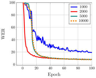
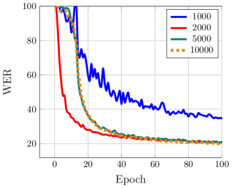
We compare the validation WER on both the clean and other conditions, for a different number of sampled words from the lexicon ${\cal D}$, as explained in Section 3.5. We report results for the CTC trained model using the Time-Depth Separable (TDS) convolution architecture of Hannun et al. (2019) with 9 TDS blocks – the acoustic model used in most of our preliminary experiments.

As we see in Figure 4, too few sampled examples makes the training unstable, and slow to converge. We do not see any advantage in having more than 5k sampled words per batch. We observe in general that the number of sampled examples may affect the beginning of training – but in our experience, when the sample set is large enough ($\geq$2000), all experiments converge to a similar word error rate.

4.2 Out-of-Vocabulary Words

Table 3: Word neighbors for selected OOVs using letter edit distance and Euclidean distance in the word model embedding space. The word model was trained with CTC on LibriSpeech 100h. The training vocabulary contains 39k words, and neighbors are computed with the full LM dictionary (200k words). Words in italic are OOV (not seen at training time).

amulet		cinderella’s		mittens		snobbish		welsh
(Edit)	(Embed.)	(Edit)	(Embed.)	(Edit)	(Embed.)	(Edit)	(Embed.)	(Edit)	(Embed.)
mulet	emulate	cinderellas	cinderellas	kittens	mattins	snobbism	snobbism	weesh	walsh
amulets	amelot	cinderella	cinderella	mitten	mittin	snobbishly	snobby	walsh	welch
amile	omelet	cantrell’s	kinsella’s	tittens	miltons	bobbish	snobbs	wesh	walch
amplest	emilet	banderillas	chaudoreille’s	ritten	middens	snobbs	snobbe	welshy	welsher
ambles	amoret	calderwell’s	ghirlandajo’s	mittin	mitten	snobbery	snobbishness	welse	wesh
mulct	amalek	kinsella’s	sganarelle’s	battens	mitton	nobis	snubby	welch	walshe
amoret	amulets	cinereous	sinclair’s	fattens	muttons	nobbs	snob’s	weals	walth
roulet	armlet	cordelia’s	cibolero’s	pattens	matins	sourish	snob	selah	welshy

In Table 1, we show that training with the complete training lexicon (89k words), and then decoding with the language model lexicon shipped with LibriSpeech (200k words) yields similar WERs as decoding with the 89k lexicon. At evaluation time, we simply extended the dictionary by computing the unseen word embeddings with the letter-based word model. We consider as out-of-vocabulary (OOV) words which are considered at inference, but not present at training time.

To further study the extent to which new words can be added to the lexicon, we trained word piece and word-level models on the “train-clean-100” subset of LibriSpeech. The lexicon for the word-level models was chosen to contain only the words which occur in the transcripts of this subset, of which there are about 34k. Given the word model receives letters as input, we compare the neighbors in the word model output embedding space to neighbors found using letter edit distance. Table 3 shows a comparison of the eight nearest neighbors for select OOV words using these two metrics. The neighbors found by the word model overlap with those found using letter edit distance. However, using only edit distance results in words which are spelled similarly but with clearly differing pronunciations as close neighbors. The word model is able to correctly discard these from the set of close neighbors. We also find that some morphology is learned by the word model (e.g. with “’s” in “cinderella’s”).

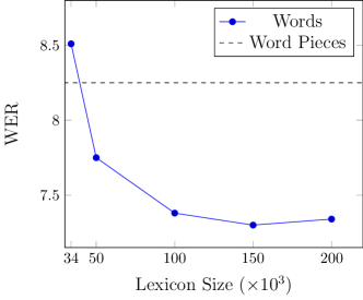
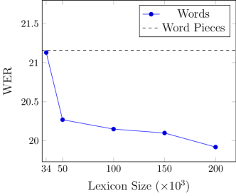
In Figure 5 we examine the word error rate as we increase the size of the lexicon used when evaluating the development set. When using the same 34k lexicon used at training time for evaluation, the word-level and word piece models perform comparably. However, as we increase the lexicon size the word-level model improves and consistently outperforms the word piece model. The larger lexicons are chosen by keeping the top words by frequency computed from the LibriSpeech language model training data.

(a) Dev clean

(b) Dev other

Figure 5: The WER on the (a) clean and (b) other development sets as a function of the lexicon size used when evaluating the word-level model. We use a 4-gram word LM for the word model and a 6-gram word piece LM for the word piece model. The word piece model uses 5k tokens but is lexicon-free.

(a) OOV Precision

(b) OOV Recall

Figure 6: Out-of-vocabulary (a) precision and (b) recall as a function of the lexicon size used when evaluating the word-level model. An OOV is any token which does not appear in the set of 34k unique tokens present in the 100 hour training set. The word piece model uses 5k tokens but is lexicon-free.

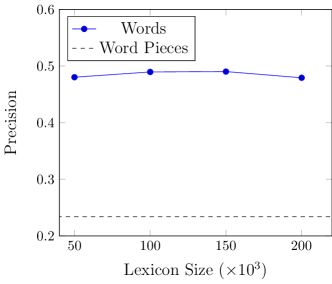
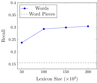
We also study the performance of the word-level and word piece models limited to out-of-vocabulary words. To do so, we first find the minimum word edit distance alignment of the models best prediction to the reference transcript. Using this alignment, we define the OOV recall as the number of correctly classified OOV words over the total number of OOVs in the reference transcripts. Similarly, we define the OOV precision as the number of correctly classified OOV words over the total number of predicted OOVs.

For example, given the reference the cat sat and the prediction cat sat we compute the following alignment (where the corresponds to a deletion):

Reference: thecatsat

Prediction: ***catsat

If both the and sat are OOV words, then the precision is $1$ and the recall is $1/2$, for this example.

For both word-level and word piece models we define an OOV as a word which does not appear in any of the training set transcriptions (i.e. any word not in the 34k lexicon). We compute OOV precision and recall on the combined clean and other development sets.

As seen in Figure 6, the word model achieves better OOV precision (a) and recall (b) than the corresponding word piece model. We also see that the word model improves in recall as we increase the lexicon size without a loss in precision. This may explain the improved word error rate of the word model with larger lexicon sizes as seen in Figure 5.

4.3 Efficiency

We compared the wall-clock time of word-based acoustic models. For decoding, the decoding time per utterance is 0.539 seconds at stride 8 (80ms), and 0.323 seconds at stride 16 (160ms). Just the forward of the acoustic model for a batch of 5 utterances takes 85ms and 60ms for stride 8 and stride 16 respectively. The whole batch (forward, criterion, backward, optimizer) takes 469ms (stride 8) vs. 426ms (stride 16), so the gain is mostly at inference time (forward). Also note that, in practice, we can fit larger batches in GPU memory with stride 16 than 8, and all in all (even with the additional FLOPS) the throughput will be higher for stride 16, but this was ran at the same batch size for comparison.

Compared to word piece models, the softmax of the word-level model is more computationally expensive at inference time. However, with a vocabulary of 89k and stride 8 model, computing the last layer represents only $11\%$ of the overall forward time (to compare with $9\%$ with a vocabulary of 10k – as in our word piece models – and $15\%$ with 200k). Word-level models have the advantage of allowing stride 16 with little loss in WER performance (see Table 1), and twice faster decoding time.

5 Conclusion

Direct-to-word speech recognition poses an exciting opportunity to simplify ASR models as well as make them more accurate and more efficient. However, this line of research has received little attention due to the difficulty of the problem. Either the model requires massive training sets to learn reasonably sized lexicons or the lexicon is small and unchangeable.

We have demonstrated that a direct-to-word approach for speech recognition is not only possible but promising. Our model gains several advantages from predicting words directly including (1) an improvement in WER over word piece baselines (2) a model which can operate at a larger stride (lower frame-rate) and hence is more efficient and (3) a simpler beam search decoder which integrates easily with an externally trained language model. Key to our approach is a letter to word embedding model which can be jointly trained with an acoustic embedding model. To make this efficient, especially for large vocabulary sizes, we used a simple sampling-based mechanism to compute the normalization term needed when training.

We have shown that our approach can be used seamlessly with two commonly used end-to-end models for speech recognition – a CTC trained model and an encoder-decoder model with attention. We validated our models on LibriSpeech, a standard benchmark in speech recognition. On this data set, the direct-to-word model achieves competitive word error rates. We also showed that the direct-to-word model has a stronger advantage over a well tuned word piece baseline in a lower resource setting. In fact, in this setting our model achieves a state-of-the-art result for end-to-end models. Finally, we demonstrated that our model can accurately predict words never seen in the training set transcriptions and gave evidence that the word-level model generalizes to out-of-vocabulary words better than a word piece model.

References

- Amodei et al. (2016) Dario Amodei, Sundaram Ananthanarayanan, Rishita Anubhai, Jingliang Bai, Eric Battenberg, Carl Case, Jared Casper, Bryan Catanzaro, Qiang Cheng, Guoliang Chen, et al. Deep speech 2: End-to-end speech recognition in english and mandarin. In International Conference on Machine Learning (ICML), pages 173–182, 2016.
- Audhkhasi et al. (2017) Kartik Audhkhasi, Bhuvana Ramabhadran, George Saon, Michael Picheny, and David Nahamoo. Direct acoustics-to-word models for english conversational speech recognition. arXiv preprint arXiv:1703.07754, 2017.
- Ba et al. (2016) Jimmy Lei Ba, Jamie Ryan Kiros, and Geoffrey E Hinton. Layer normalization. arXiv preprint arXiv:1607.06450, 2016.
- Bahdanau et al. (2014) Dzmitry Bahdanau, Kyunghyun Cho, and Yoshua Bengio. Neural machine translation by jointly learning to align and translate. In International Conference on Learning Representations (ICLR), 2014.
- Bahdanau et al. (2016) Dzmitry Bahdanau, Jan Chorowski, Dmitriy Serdyuk, Philemon Brakel, and Yoshua Bengio. End-to-end attention-based large vocabulary speech recognition. In International Conference on Acoustics, Speech and Signal Processing (ICASSP), pages 4945–4949. IEEE, 2016.
- Bengio and Heigold (2014) Samy Bengio and Georg Heigold. Word embeddings for speech recognition. In Fifteenth Annual Conference of the International Speech Communication Association, 2014.
- Bisani and Ney (2008) Maximilian Bisani and Hermann Ney. Joint-sequence models for grapheme-to-phoneme conversion. Speech communication, 50(5):434–451, 2008.
- Bojanowski et al. (2017) Piotr Bojanowski, Edouard Grave, Armand Joulin, and Tomas Mikolov. Enriching word vectors with subword information. Transactions of the Association for Computational Linguistics, 5:135–146, 2017.
- Chan et al. (2016) William Chan, Navdeep Jaitly, Quoc Le, and Oriol Vinyals. Listen, attend and spell: A neural network for large vocabulary conversational speech recognition. In Acoustics, Speech and Signal Processing (ICASSP), 2016 IEEE International Conference on, pages 4960–4964. IEEE, 2016.
- Cho et al. (2014) Kyunghyun Cho, Bart Van Merriënboer, Caglar Gulcehre, Dzmitry Bahdanau, Fethi Bougares, Holger Schwenk, and Yoshua Bengio. Learning phrase representations using rnn encoder-decoder for statistical machine translation. 2014.
- Collobert et al. (2016) Ronan Collobert, Christian Puhrsch, and Gabriel Synnaeve. Wav2letter: an end-to-end convnet-based speech recognition system. arXiv preprint arXiv:1609.03193, 2016.
- Collobert et al. (2019) Ronan Collobert, Awni Hannun, and Gabriel Synnaeve. A fully differentiable beam search decoder. In International Conference on Machine Learning (ICML), 2019.
- Dauphin et al. (2017) Yann N Dauphin, Angela Fan, Michael Auli, and David Grangier. Language modeling with gated convolutional networks. In International Conference on Machine Learning (ICML), pages 933–941, 2017.
- Fan et al. (2019) Angela Fan, Edouard Grave, and Armand Joulin. Reducing transformer depth on demand with structured dropout. arXiv preprint arXiv:1909.11556, 2019.
- Gibson and Hain (2006) Matthew Gibson and Thomas Hain. Hypothesis spaces for minimum bayes risk training in large vocabulary speech recognition. In Ninth international conference on spoken language processing, 2006.
- Graves and Jaitly (2014) Alex Graves and Navdeep Jaitly. Towards end-to-end speech recognition with recurrent neural networks. In International Conference on Machine Learning (ICML), pages 1764–1772, 2014.
- Graves et al. (2006) Alex Graves, Santiago Fernández, Faustino Gomez, and Jürgen Schmidhuber. Connectionist temporal classification: labelling unsegmented sequence data with recurrent neural networks. In International Conference on Machine Learning (ICML), pages 369–376, 2006.
- Hannun et al. (2019) Awni Hannun, Ann Lee, Qiantong Xu, and Ronan Collobert. Sequence-to-sequence speech recognition with time-depth separable convolutions. arXiv preprint arXiv:1904.02619, 2019.
- Irie et al. (2019) Kazuki Irie, Rohit Prabhavalkar, Anjuli Kannan, Antoine Bruguier, David Rybach, and Patrick Nguyen. On the choice of modeling unit for sequence-to-sequence speech recognition. In Interspeech, 2019.
- Kanthak and Ney (2002) Stephan Kanthak and Hermann Ney. Context-dependent acoustic modeling using graphemes for large vocabulary speech recognition. In 2002 IEEE International Conference on Acoustics, Speech, and Signal Processing, volume 1, pages I–845. IEEE, 2002.
- Killer et al. (2003) Mirjam Killer, Sebastian Stuker, and Tanja Schultz. Grapheme based speech recognition. In Eighth European Conference on Speech Communication and Technology, 2003.
- Kim et al. (2016) Yoon Kim, Yacine Jernite, David Sontag, and Alexander M Rush. Character-aware neural language models. In Thirtieth AAAI conference on artificial intelligence, 2016.
- Kudo and Richardson (2018) Taku Kudo and John Richardson. SentencePiece: A simple and language independent subword tokenizer and detokenizer for neural text processing. arXiv preprint arXiv:1808.06226, 2018.
- Labeau and Allauzen (2017) Matthieu Labeau and Alexandre Allauzen. Character and subword-based word representation for neural language modeling prediction. In Proceedings of the First Workshop on Subword and Character Level Models in NLP, pages 1–13, 2017.
- Li et al. (2018) Jinyu Li, Guoli Ye, Amit Das, Rui Zhao, and Yifan Gong. Advancing acoustic-to-word ctc model. In 2018 IEEE International Conference on Acoustics, Speech and Signal Processing (ICASSP), pages 5794–5798. IEEE, 2018.
- Likhomanenko et al. (2019) Tatiana Likhomanenko, Gabriel Synnaeve, and Ronan Collobert. Who needs words? lexicon-free speech recognition. arXiv preprint arXiv:1904.04479, 2019.
- Ling et al. (2015a) Wang Ling, Tiago Luís, Luís Marujo, Ramón Fernandez Astudillo, Silvio Amir, Chris Dyer, Alan W Black, and Isabel Trancoso. Finding function in form: Compositional character models for open vocabulary word representation. arXiv preprint arXiv:1508.02096, 2015a.
- Ling et al. (2015b) Wang Ling, Isabel Trancoso, Chris Dyer, and Alan W Black. Character-based neural machine translation. arXiv preprint arXiv:1511.04586, 2015b.
- Lüscher et al. (2019) Christoph Lüscher, Eugen Beck, Kazuki Irie, Markus Kitza, Wilfried Michel, Albert Zeyer, Ralf Schlüter, and Hermann Ney. Rwth asr systems for librispeech: Hybrid vs attention-w/o data augmentation. In Interspeech, 2019.
- Maas et al. (2015) Andrew Maas, Ziang Xie, Dan Jurafsky, and Andrew Ng. Lexicon-free conversational speech recognition with neural networks. In Proceedings of the 2015 Conference of the North American Chapter of the Association for Computational Linguistics: Human Language Technologies, pages 345–354, 2015.
- Panayotov et al. (2015) Vassil Panayotov, Guoguo Chen, Daniel Povey, and Sanjeev Khudanpur. Librispeech: an asr corpus based on public domain audio books. In 2015 IEEE International Conference on Acoustics, Speech and Signal Processing (ICASSP), pages 5206–5210. IEEE, 2015.
- Park et al. (2019) Daniel S Park, William Chan, Yu Zhang, Chung-Cheng Chiu, Barret Zoph, Ekin D Cubuk, and Quoc V Le. Specaugment: A simple data augmentation method for automatic speech recognition. In Interspeech, 2019.
- Prabhavalkar et al. (2018) Rohit Prabhavalkar, Tara N Sainath, Yonghui Wu, Patrick Nguyen, Zhifeng Chen, Chung-Cheng Chiu, and Anjuli Kannan. Minimum word error rate training for attention-based sequence-to-sequence models. In International Conference on Acoustics, Speech and Signal Processing (ICASSP), pages 4839–4843. IEEE, 2018.
- Pratap et al. (2018) Vineel Pratap, Awni Hannun, Qiantong Xu, Jeff Cai, Jacob Kahn, Gabriel Synnaeve, Vitaliy Liptchinsky, and Ronan Collobert. wav2letter++: The fastest open-source speech recognition system. arXiv preprint arXiv:1812.07625, 2018.
- Rao et al. (2015) Kanishka Rao, Fuchun Peng, Haşim Sak, and Françoise Beaufays. Grapheme-to-phoneme conversion using long short-term memory recurrent neural networks. In 2015 IEEE International Conference on Acoustics, Speech and Signal Processing (ICASSP), pages 4225–4229. IEEE, 2015.
- Santos and Zadrozny (2014) Cicero D Santos and Bianca Zadrozny. Learning character-level representations for part-of-speech tagging. In Proceedings of the 31st International Conference on Machine Learning (ICML-14), pages 1818–1826, 2014.
- Settle et al. (2019) Shane Settle, Kartik Audhkhasi, Karen Livescu, and Michael Picheny. Acoustically grounded word embeddings for improved acoustics-to-word speech recognition. In 2015 IEEE International Conference on Acoustics, Speech and Signal Processing (ICASSP). IEEE, 2019.
- Soltau et al. (2016) Hagen Soltau, Hank Liao, and Hasim Sak. Neural speech recognizer: Acoustic-to-word lstm model for large vocabulary speech recognition. arXiv preprint arXiv:1610.09975, 2016.
- Sutskever et al. (2014) Ilya Sutskever, Oriol Vinyals, and Quoc V Le. Sequence to sequence learning with neural networks. In Advances in neural information processing systems (NIPS), pages 3104–3112, 2014.
- Synnaeve et al. (2019) Gabriel Synnaeve, Qiantong Xu, Jacob Kahn, Edouard Grave, Tatiana Likhomanenko, Vineel Pratap, Anuroop Sriram, Vitaliy Liptchinsky, and Ronan Collobert. End-to-end asr: from supervised to semi-supervised learning with modern architectures. arXiv preprint arXiv:1911.08460, 2019.
- Vaswani et al. (2017) Ashish Vaswani, Noam Shazeer, Niki Parmar, et al. Attention is all you need. In Adv. NIPS, 2017.
- Zeyer et al. (2018) Albert Zeyer, Kazuki Irie, Ralf Schlüter, and Hermann Ney. Improved training of end-to-end attention models for speech recognition. arXiv preprint arXiv:1805.03294, 2018.