Full counting statistics of energy transfers in inhomogeneous nonequilibrium states of $(1+1)D$ CFT

Abstract

Employing the conformal welding technique, we find an exact expression for the Full Counting Statistics of energy transfers in a class of inhomogeneous nonequilibrium states of a (1+1)-dimensional unitary Conformal Field Theory. The expression involves the Schwarzian action of a complex field obtained by solving a Riemann-Hilbert type problem related to conformal welding of infinite cylinders. On the way, we obtain a formula for the extension of characters of unitary positive-energy representations of the Virasoro algebra to 1-parameter groups of circle diffeomorphisms and we develop techniques, based on the analysis of certain classes of Fredholm operators, that allow to control the leading asymptotics of such extensions for small real part of the modular parameter $\,\tau$.

1 Introduction

$(1+1)D$ Conformal Field Theory (CFT) provides an effective description of long-range physics in a number of critical systems in one spatial dimension. The examples include electrons or cold atoms trapped in one-dimensional potential wells, carbon nanotubes, quantum Hall edge currents or critical XXZ spin chains. CFT permitted to explain the long-range equilibrium properties of such systems that are driven by the low lying excitations but, more recently, it has also been used to describe the nonequilibrium situations, like the evolution after quantum quenches CaCa2 or in the partitioning protocol after two haft-line systems prepared in different equilibrium states are joined together BD2 . In LLMM2 a smooth version of the partitioning protocol was considered for nonlocal and local Luttinger model Lutt ; ML of interacting fermions with the initial nonequilibrium state possessing a built-in inverse-temperature profile $\,\beta(x)\,$ interpolating smoothly between different constant values on the left and on the right. More exactly, such a profile state corresponds in finite box of length of order $\,L\,$ to the density matrix proportional to $\,\exp[-G_{L}]\,$ where $\,G_{L}=\int\beta(x){\cal E}(x)\hskip 0.71114ptdx\,$ with $\,{\cal E}(x)\,$ standing for the energy density and the integral running over the box. The evolution of the energy density and current in such an initial state was computed in LLMM2 in the $\,L\to\infty\,$ limit in the perturbation theory in the difference of the asymptotic values of the inverse-temperature profile, for the local version of the model to all orders. The local Luttinger model is a $(1+1)D$ CFT and in GLM the evolution of similar profile states was analyzed for a general unitary $(1+1)D$ CFT using global conformal symmetries of the theory. The latter permitted to reduce the arbitrary correlation functions of the energy-momentum components or the primary fields in the nonequilibrium profile states to equilibrium correlation functions, considerably generalizing the results of LLMM2 on the local Luttinger model.

The present paper is, in a sense, a continuation of GLM . We show how global conformal symmetries may be used to provide an exact expression for the generating function for Full Counting Statistics (FCS) of energy transfers through a kink in the profile of a profile state. The notion of FCS was introduced by L. S. Levitov and G. B. Lesovik in LL , where an exact formula for the generating function for FCS of charge transport between free-fermion channels was obtained. For finite volumes, the expression involves Fredholm determinants containing scattering amplitudes ABGK . The definition of FCS requires a measurement protocol for the changes of the conserved quantity which may be assimilated with its transfers. The measurements may be indirect, performed on a device coupled to the system LLL , or direct, performed on the system in question, MA . Our approach to FCS of energy transfers in a profile state will be based on the two-time measurement protocol that belongs to the latter class. We shall extract the energy transfer through the kink in $\,\beta(x)\,$ from two measurements, separated by time $\,t$,  of the finite box observable $\,G_{L}\,$ introduced above. To associate the difference of the results of such measurements with the energy transfer through the kink encompassed by the spatial box, we shall have to impose boundary conditions that guarantee that there is no energy transfer through the edges of the box. Those are different from the periodic boundary conditions used in GLM . The finite-volume CFT with such boundary conditions is chiral, i.e. its space of states carries a unitary, positive-energy representation of a single Virasoro algebra with generators $\,L_{n}\,$ and central charge $\,c$.  The Virasoro representation lifts to a projective unitary representation of the group $\,{Diff_{+}S^{1}}\,$ of smooth, orientation-preserving diffeomorphisms of the circle. We show that the generating function for FCS of energy transfers extracted from the two-time measurements of $\,G_{L}\,$ may be expressed in terms of the character

$$\Upsilon(f,\tau)=\hbox{Tr}\Big{(}U(f)\,{\rm e}^{2\pi\mathrm{i}\tau(L_{0}-\frac{c}{24})}\Big{)}$$ (1.1)

of the projective representation $\,f\mapsto U(f)\,$ of $\,{Diff_{+}S^{1}}$,  where $\,\tau\,$ is in the upper half-plane. In fact one only needs to know such a character on 1-parameter subgroups $\,(f_{s})\,$ of $\,{Diff_{+}S^{1}}$.  Unlike the Virasoro characters $\,\chi(\tau)\,$ defined by a similar formula but with $\,U(f)\,$ absent, the characters $\,\Upsilon(f,\tau)\,$ have not been studied in detail. Inspired by the recent work FH2 , which used conformal welding of boundaries of two discs with a twist by the circle diffeomorphism $\,f_{s}\,$ to express the vacuum matrix elements $\,\langle 0|U(f_{s})|0\rangle$,  see also Poly ,  we obtain an exact formula for $\,\Upsilon(f_{s},\tau)\,$ from conformal welding with the twist by $\,f_{s}$ of the boundaries of complex annulus $\,\{z\,|\,|{\rm e}^{2\pi\mathrm{i}\tau}|\leq|z|\leq 1\}$.  In fact, following the approach of Segal , one of the present authors (K.G.) has previously obtained a general formula for $\,\Upsilon(f,\tau)\,$ involving Fredholm determinants of operators appearing in a Riemann-Hilbert type problem underlying the same conformal welding construction KGr . The approach based on the idea of FH2 , that we describe here, produces, however, a simpler integral expression for $\,\Upsilon(f_{s},\tau)$. This reduction resembles the use of a Riemann-Hilbert problem solution in MA in the context of the Levitov-Lesovik formula. In our case, the generating function for finite-volume FCS is finally expressed by a ratio of Virasoro characters at two different values of $\,\tau\,$ and the exponential of an integral involving the Schwarzian derivative of a solution of a Fredholm equation directly related to conformal welding of the boundaries of annuli.

In the infinite-volume limit, whose rigorous control is somewhat cumbersome, the expression for the generating function for FCS simplifies to the exponential of an integral involving the solution of a Fredholm equation now related to conformal welding of the boundaries of an infinite strip in the complex plane or, equivalently, of the boundaries of two discs. The corresponding Fredholm equation may be studied numerically as discussed in ShM . The infinite-volume result exhibits a large degree of universality: the generating function for FCS depends only on the profile $\,\beta(x)\,$ and on the central charge $\,c\,$ that enters as an overall power, but not on the details of the CFT. For large times $\,t$,  the generating function for FCS should take the large deviations form derived in BD0 for the partitioning protocol. That form depends on $\,\beta(x)\,$ only through the asymptotic values. It arises when conformal welding of the strip boundaries involves the diffeomorphism that is a simple translation but we still lack a sufficient rigorous control of the large $\,t\,$ asymptotics of the finite-time Fredholm equation so that the large-deviations result remains only heuristic at the moment.

The reference GLM considered also nonequilibrium states with profiles for both the inverse temperature and the chemical potential in CFTs with the $\,u(1)\,$ current algebra. The approach to FCS discussed here may be extended to cover the $\,u(1)$-charge transfers at least in states with chemical potential profile but constant $\,\beta$. We postpone the study of such extensions to a future publication.

The present paper is organized as follows. In Sec. 2, we describe the structure of $(1+1)D$ CFT in a finite box with no energy-flux through the boundary. Sec. 3 gives three simple examples of such CFTs: the free massless fermions (Sec. A), the free massless compactified bosons (Sec. B), and the local Luttinger model (Sec. C). In Sec. 4, we construct the finite-volume non-equilibrium profile states (Sec. A), show how they may be related to equilibrium states (Sec. B), and discuss their infinite-volume limit that coincides with the one obtained in ref. GLM which used periodic boundary conditions (Sec. C). Sec. 5 contains a preliminary discussion of FCS of energy transfers in the profiles states, describing the two-time measurement protocol for FCS (Sec. A) and defining the FCS generating function (Sec. B). Sec. 6, that constitutes the core of the paper, relates FCS to conformal welding. First, we express the generating function of finite-volume FCS via characters of $\,{Diff_{+}S^{1}}\,$ (Sec. A). Next, we explain a correspondence between $\,{Diff_{+}S^{1}}\,$ and Virasoro characters that originates from the isomorphism between tori which are conformally welded from annuli with and without twist by a circle diffeomorphism (Sec. B). Then we discuss the connection between conformal welding of tori and an inhomogeneous Riemann-Hilbert problem (Sec. C). Next, we obtain a relation between the 1-point function of the Euclidian energy-momentum tensor on the tori welded with and without twist (Sec. D). Such a relation gives rise to a formula for $\,{Diff_{+}S^{1}}$-characters on 1-parameter subgroups (Sec. E) and for the correspondence between modular parameters of tori welded with and without twist (Sec. F). Finally, we apply the above formulae to obtain an exact expression for the generating function for finite-volume FCS (Sec. G). The infinite-volume limit of that expression is discussed in Sec. 7. First, we study the infinite-volume behavior of the 1-parameter subgroups of circle diffeomorphisms providing twists for conformal welding of tori on which the finite-volume FCS formula was based (Sec. A). Next, we discuss conformal welding of cylinders to which conformal welding of tori reduces in the infinite-volume limit (Sec. B). Based on that, we extract, under some technical assumptions, our exact infinite-volume formula for the generating function for FCS of energy transfers (Sec. C) and check that it represents correctly the first two moments of the energy transfer (Sec. D). Sec. 8 examines the long-time large-deviations asymptotics for FCS of energy transfers and discusses its consequences that were first pointed out in BD0 . Sec. 9 is devoted to a rigorous proof of the technical assumptions used in Sec. 7 about the the convergence of solutions of the Fredholm equations related to conformal welding of tori and of cylinders. This is the most technical part of the paper and it uses results developed in Appendix C about Fredholm operators of two classes relevant for our problem, their determinants and their inverses. Finally,  Sec. 10  lists our conclusions and other Appendices A,B,D,E and F establish few more technical results used on the way.

Acknowledgements.  K.G. thanks Chris Fewster and Stefan Hollands for inspiring discussions and Jan Dereziński, Stefan Hollands and Karl-Henning Rehren for an invitation to the BIRS 2018 workshop “Physics and Mathematics of Quantum Field Theory” that influenced the work on the present paper.

2 Minkowskian CFT in a finite box

Let us consider a Minkowskian CFT in the spatial box $\,[-{\frac{{}_{1}}{{}^{4}}L},{\frac{{}_{1}}{{}^{4}}L}]\,$ with a special type of boundary conditions that assure the following gluing relations for the right- and left-moving components $\,T_{+}(x^{-})\,$ and $\,T_{-}(x^{+})\,$ of the energy-momentum tensor:

$$T_{+}(x^{-})=T_{-}(x^{+})\qquad{\rm for}\qquad x=\pm{\frac{{}_{1}}{{}^{4}}L}\,,$$ (2.1)

where $\,x^{\pm}=x\pm vt\,$ are the light-cone coordinates. The latter relations mean that there is no energy flux through the boundary and they imply that $\,T_{+}(x)\,$ and $\,T_{-}(x)\,$ are $\,L$-periodic distributions with values in self-adjoint operators in the Hilbert space $\,{\cal H}_{L}\,$ of states of the finite-box theory satisfying the relation

$$T_{-}(x)=T_{+}(-x\pm\frac{{}_{1}}{{}^{2}}L)\,.$$ (2.2)

Such a theory is then chiral: there is just one independent $\,L$-periodic component of the energy-momentum tensor for which we shall choose $\,T_{+}(x)\equiv T(x)$.  The Fourier modes of $\,T(x)\,$ define the generators $\,L_{n},\ n\in\mathbb{Z}$,  of the Virasoro algebra

$$T(x)=\frac{{}_{2\pi}}{{}^{L^{2}}}\sum\limits_{n=-\infty}^{\infty}{\rm e}^{\frac{2\pi\mathrm{i}n}{L}(x+\frac{1}{4}L)}\big{(}L_{n}-\frac{{}_{c}}{{}^{24}}\delta_{n,0}\big{)}\,,$$ (2.3)

with $\,L_{n}=L_{-n}^{\dagger}\,$ satisfying (on a common dense domain) the commutation relations

$$[L_{n},L_{m}]=(n-m)L_{n+m}+\frac{{}_{c}}{{}^{12}}(n^{3}-n)\delta_{n,-m}$$ (2.4)

which are equivalent to

$$[T(x),T(y)]=-2\mathrm{i}\,\delta^{\prime}_{L}(x-y)\,T(y)+\mathrm{i}\,\delta_{L}(x-y)\,T^{\prime}(y)+\frac{{}_{c\,\mathrm{i}}}{{}^{24\pi}}\,\delta^{\prime\prime\prime}_{L}(x-y)\,,$$ (2.5)

where $\,c\,$ is the central charge of the theory and $\,\delta_{L}\,$ is the $L$-periodized delta-function. We assume that the Hilbert space of states $\,{\cal H}_{L}\,$ of the finite-box theory is a (possibly infinite) direct sum of the unitary highest-weight representations of the Virasoro algebra with fixed central charge $\,c\,$ containing the vacuum representation exactly once.

The energy density of the theory is defined by

$${\cal E}(t,x)=v\big{(}T_{+}(x^{-})+T_{-}(x^{+})\big{)}=v\big{(}T(x^{-})+T(-x^{+}-\frac{{}_{1}}{{}^{2}}L)\big{)}\,,\qquad$$ (2.6)

and the self-adjoint Hamiltonian in the box is

$$H_{L}\,=\,\int_{-{\frac{{}_{1}}{{}^{4}}L}}^{{\frac{{}_{1}}{{}^{4}}L}}{\cal E}(t,x)\,dx\,=\,v\int_{-{\frac{{}_{3}}{{}^{4}}L}}^{{\frac{{}_{1}}{{}^{4}}L}}T(x^{-})\,dx\,=\,\frac{{}_{2\pi v}}{{}^{L}}\big{(}L_{0}-\frac{{}_{c}}{{}^{24}}\big{)}.$$ (2.7)

It generates the right-moving dynamics of $\,T(x)$:

$${\rm e}^{\mathrm{i}tH_{L}}T(x)\,{\rm e}^{-\mathrm{i}tH_{L}}\,=\,T(x^{-})\,.$$ (2.8)

We assume additionally that $\,\hbox{Tr}\,\big{(}{\rm e}^{-\beta_{0}H_{L}}\big{)}<\infty\,$ for all $\,\beta_{0}>0$,  a condition that is satisfied for a rich class of models of CFT including the rational ones. The expectation values of observables in the finite-box equilibrium state with inverse temperature $\,\beta_{0}\,$ are then defined by the formula

$$\big{\langle}A\big{\rangle}_{\beta_{0};L}^{\rm eq}\,=\,\frac{\hbox{Tr}\,\big{(}A\,{\rm e}^{-\beta_{0}H_{L}}\big{)}}{\hbox{Tr}\,\big{(}{\rm e}^{-\beta_{0}H_{L}}\big{)}}$$ (2.9)

(we set $\,\hbar=1=k_{B}$).

Let $\,{Diff_{+}S^{1}}\,$ be the group of smooth, orientation-preserving diffeomorphisms of the circle $\,S^{1}_{L}=\mathbb{R}/L\mathbb{Z}\,$ and let $\,{Diff_{+}{}^{{}^{\sim}}S^{1}}\,$ be its universal cover.  Elements of $\,{Diff_{+}{}^{{}^{\sim}}S^{1}}\,$ are smooth functions $\,f:\mathbb{R}\to\mathbb{R}\,$ such that $\,f^{\prime}(x)>0\,$ and $\,f(x+L)=f(x)+L$.  The group $\,{Diff_{+}{}^{{}^{\sim}}S^{1}}\,$ is contractible and one has the central extension of groups

$$0\,\longrightarrow\,\mathbb{Z}\,\longrightarrow\,{Diff_{+}{}^{{}^{\sim}}S^{1}}\,\longrightarrow\,{Diff_{+}S^{1}}\,\longrightarrow\,1$$ (2.10)

where $\,n\in\mathbb{Z}\,$ is represented by the translation $\,x\mapsto x+nL$.  (Direct sums of) unitary highest-weight representations of the Virasoro algebra with central charge $\,c\,$ lift to unitary projective representations $\,f\mapsto U(f)\,$ of $\,{Diff_{+}{}^{{}^{\sim}}S^{1}}\,$ [GW2, ,TL, ,FH1, ]  such that,

$$U(f)\,T(x)\,U(f)^{-1}\,=\,f^{\prime}(x)^{2}\,T(f(x))-\frac{c}{{24\pi}}(Sf)(x)\,,$$ (2.11)

where

$$(Sf)(x)=\frac{f^{\prime\prime\prime}(x)}{f^{\prime}(x)}-\frac{3}{2}\Big{(}\frac{f^{\prime\prime}(x)}{f^{\prime}(x)}\Big{)}^{2}$$ (2.12)

is the Schwarzian derivative of $\,f\,$ fulfilling the chain rule

$$S(f_{1}\circ f_{2})=(f_{2}^{\prime})^{2}(Sf_{1})\circ f_{2}\,+\,Sf_{2}\,.$$ (2.13)

If $\,\zeta:\mathbb{R}\rightarrow\mathbb{R}\,$ is a smooth function satisfying $\,\zeta(x+L)=\zeta(x)\,$ defining a vector field $\,-\zeta(x)\partial_{x}\,$ on $\,\mathbb{R}\,$ and if $\,f_{s}(x)\,$ is the flow of the latter that forms a 1-parameter subgroup of $\,{Diff_{+}{}^{{}^{\sim}}S^{1}}$,  i.e.

$$\partial_{s}f_{s}(x)=-\zeta(f_{s}(x))\,,\qquad f_{0}(x)=x\,,$$ (2.14)

then

$$U(f_{s})=c_{s,\zeta}\,\exp\Big{[}\mathrm{i}s\int_{-{\frac{{}_{3}}{{}^{4}}L}}^{{\frac{{}_{1}}{{}^{4}}L}}\zeta(x)T(x)dx\Big{]},$$ (2.15)

where $\,|c_{s,\zeta}|=1$.  In particular, if $\,\zeta(x)=L\,$ then $\,f_{s}(x)=x-sL\,$ are translations that form the Cartan subgroup of $\,{Diff_{+}{}^{{}^{\sim}}S^{1}}\,$ and

$$U(f_{s})=c_{s,L}\,{\rm e}^{2\pi\mathrm{i}s(L_{0}-\frac{c}{24})}\hskip 0.71114pt.$$ (2.16)

The projective factors in $\,U(f)\,$ may be fixed so that FH1

$$U(f_{1})\hskip 0.71114ptU(f_{2})=\exp\Big{[}\frac{\mathrm{i}c}{48\pi}\int_{-{\frac{{}_{3}}{{}^{4}}L}}^{{\frac{{}_{1}}{{}^{4}}L}}\ln{(f_{1}\circ f_{2})^{\prime}(x)}\,d\ln{f_{2}^{\prime}(x)}\Big{]}U(f_{1}\circ f_{2})\,.$$ (2.17)

The exponential term on the right-hand side of (2.17) defines the Bott 2-cocycle on $\,{Diff_{+}{}^{{}^{\sim}}S^{1}}\,$ that corresponds to the infinitesimal 2-cocycle given by the last terms on the right-hand side of (2.4) or (2.5) KhWe .

Eqs. (2.11) and (2.2) imply that in the special case when

$$f(-x-\frac{{}_{1}}{{}^{2}}L)=-f(x)-\frac{{}_{1}}{{}^{2}}L$$ (2.18)

one also has the relation

$$U(f)\,T_{-}(x)\,U(f)^{-1}\,=\,f^{\prime}(x)^{2}\,T_{-}(f(x))-\frac{c}{{24\pi}}(Sf)(x)\,.$$ (2.19)

The projective representation $\,f\rightarrow U(f)\,$ in the Hilbert space $\,{\cal H}_{L}\,$ of the finite-box theory will be our main tool used below.

The primary fields $\,\Phi(x,t)\,$ satisfy in the light-cone re parameterization the commutation relations

$$[T(x),\Phi(y^{-},y^{+})] = -\mathrm{i}\big{(}\Delta^{+}_{\Phi}\delta^{\prime}_{L}(x-y^{-})+\Delta^{-}_{\Phi}\delta^{\prime}_{L}(x+y^{+}+\frac{{}_{1}}{{}^{2}}L)\big{)}\Phi(y^{-},y^{+})$$ (2.22)

$$+\mathrm{i}\,\delta_{L}(x-y^{-})\,\partial_{-}\Phi(y^{-},y^{+})-\mathrm{i}\,\delta_{L}(x+y^{+}+\frac{{}_{1}}{{}^{2}}L)\,\partial_{+}\Phi(y^{-},y^{+})\,,$$

where $\,(\Delta^{+}_{\Phi},\Delta^{-}_{\Phi})\,$ are the conformal weights of $\,\Phi$.  Under the adjoint action of $\,U(f)\,$ for $\,f\in{Diff_{+}{}^{{}^{\sim}}S^{1}}\,$ they transform according to the rule

$$U(f)\hskip 0.71114pt\Phi(x^{-},x^{+})\hskip 0.71114ptU(f)^{-1}=f^{\prime}(x^{-})^{\Delta^{+}_{\Phi}}f^{\prime}(-x^{+}-\frac{{}_{1}}{{}^{2}}L)^{\Delta^{-}_{\Phi}}\,\Phi(f(x^{-}),-f(-x^{+}-\frac{{}_{1}}{{}^{2}}L)-\frac{{}_{1}}{{}^{2}}L)$$ (2.23)

that simplifies to

$$U(f)\hskip 0.71114pt\Phi(x^{-},x^{+})\hskip 0.71114ptU(f)^{-1}=f^{\prime}(x^{-})^{\Delta^{+}_{\Phi}}f^{\prime}(x^{+})^{\Delta^{-}_{\Phi}}\,\Phi(f(x^{-}),f(x^{+}))$$ (2.24)

if $\,f\,$ satisfies (2.18).

3 Simple examples

For illustration, we list three simple examples of models of CFT with the structure as discussed above. Many other examples, e.g., the unitary minimal models or the WZW and coset theories, may be added to that list.

A Free massless fermions

The classical action functional of anti-commuting Fermi fields has here the form

$$S[\psi_{+},\psi_{-}]\,=\,\frac{{}_{2\mathrm{i}v}}{{}^{\pi}}\int dt\int_{-{\frac{{}_{1}}{{}^{4}}L}}^{{\frac{{}_{1}}{{}^{4}}L}}\big{[}\psi_{+}^{*}\partial_{+}\psi_{+}\,-\,\psi_{-}^{*}\partial_{-}\psi_{-}\big{]}dx\,,$$ (3.1)

where $\,\partial_{\pm}=\frac{1}{2}(\partial_{x}\pm v^{-1}\partial_{t})$.  We impose on the fields the boundary conditions

$$\psi_{+}(t,-\frac{{}_{1}}{{}^{4}}L)=\psi_{-}(t,-\frac{{}_{1}}{{}^{4}}L)\,,\qquad\psi_{+}(t,\frac{{}_{1}}{{}^{4}}L)=-\psi_{-}(t,\frac{{}_{1}}{{}^{4}}L)\,.$$ (3.2)

The quantized theory has the fermionic Fock space $\,{\cal F}_{f}\,$ carrying the vacuum representation of CAR

$$[c_{p},c_{p^{\prime}}]_{{}_{+}}=0=[c^{\dagger}_{p},c^{\dagger}_{p^{\prime}}]_{{}_{+}},\qquad[c_{p},c^{\dagger}_{p^{\prime}}]_{{}_{+}}=\delta_{p,p^{\prime}}$$ (3.3)

with $\,p,p^{\prime}\in\frac{1}{2}+\mathbb{Z}\,$ as the space of states $\,{\cal H}_{L}$,  with the normalized Dirac vacuum $\,|0\rangle_{f}\,$ annihilated by $\,c_{p}\,$ and $\,c^{\dagger}_{-p}\,$ with $\,p>0$.  The quantum fermionic fields are

$$\psi_{\pm}(t,x)=\sqrt{\frac{{}_{\pi}}{{}^{L}}}\hskip 0.71114pt\sum\limits_{p}c_{p}\,{\rm e}^{\pm\frac{2\pi\mathrm{i}p}{L}(x^{\mp}+\frac{1}{4}L)}\,\equiv\,\psi_{\pm}(x^{\mp})$$ (3.4)

and the energy momentum tensor components

$$T_{\pm}(x^{\mp})=\pm\frac{{}_{\mathrm{i}}}{{}^{2\pi}}:\big{(}(\partial_{\mp}\psi^{\dagger}_{\pm})\psi_{\pm}-\psi_{\pm}^{\dagger}\partial_{\mp}\psi_{\pm}\big{)}(x^{\mp}):-\frac{{}_{\pi c}}{{}^{12L^{2}}}$$ (3.5)

satisfy (2.1) and correspond to $\,c=1\,$ Virasoro generators

$$L_{n}=\sum\limits_{p}(p-\frac{{}_{n}}{{}^{2}}):c_{p-n}^{\dagger}c_{p}:$$ (3.6)

where the fermionic Wick ordering $\,:-:\,$ puts the creators $\,c_{p}\,$ and $\,c^{\dagger}_{-p}\,$ with $\,p<0\,$ to the left of the annihilators, with a minus sign for each transposition. $\,\psi_{\pm}(x^{\mp})\,$ are primary fields with the conformal weights $\,(\frac{1}{2},0)\,$ and $\,(0,\frac{1}{2})$,  respectively,  and so are their hermitian conjugates $\,\psi_{\pm}^{\dagger}(x^{\mp})$.  Among the other primary fields of the theory there are the chiral components of the $\,U(1)$ current

$$J_{\pm}(x^{\mp})=\frac{{}_{1}}{{}^{\pi}}:(\psi^{\dagger}_{\pm}\psi_{\pm})(x^{\mp}):$$ (3.7)

with conformal weights $\,(1,0)\,$ and $\,(0,1)$,  respectively.

B Compactified free massless bosons

The classical action functional of the massless free field $\,\varphi(x,t)\,$ with values defined modulo $\,2\pi\,$ is

$$S[\varphi]=\frac{{}_{r^{2}}}{{}^{4\pi}}\int dt\int_{-{\frac{{}_{1}}{{}^{4}}L}}^{{\frac{{}_{1}}{{}^{4}}L}}\big{[}(\partial_{t}\varphi)^{2}-(\partial_{x}\varphi)^{2}\big{]}\,dx\,.$$ (3.8)

The parameter $\,r\,$ has the interpretation of the radius of compactification of the circle of values of the field. We impose on the fields $\,\varphi(x,t)\,$ the Neumann boundary conditions

$$\partial_{x}\varphi(t,-\frac{{}_{1}}{{}^{4}}L)=0=\partial_{x}\varphi(t,\frac{{}_{1}}{{}^{4}}L)\,.$$ (3.9)

The space of states $\,{\cal H}_{L}\,$ of the quantized theory is then the tensor product $\,{\cal H}_{0}\otimes{\cal F}_{b}$.  The second factor is the bosonic Fock space $\,{\cal F}_{b}\,$ carrying the vacuum representation of the CCR algebra

$$[\alpha_{n},\alpha_{m}]=n\hskip 0.71114pt\delta_{n,-m}$$ (3.10)

for $\,n\in\mathbb{Z}$,  with the normalized vacuum state $\,|0\rangle_{b}\,$ annihilated by $\,\alpha_{n}\,$ for $\,n\geq 0\,$ and with $\,\alpha_{-n}=\alpha_{n}^{\dagger}$. The mode $\,\alpha_{0}$,  that commutes with all $\,\alpha_{n}$,  acts in the zero-mode space $\,{\cal H}_{0}\,$ spanned by the orthonormal vectors $\,|k\rangle,\,k\in\mathbb{Z}$,  by

$$\alpha_{0}|k\rangle=\frac{{}_{\sqrt{2}}}{{}^{r}}k\hskip 0.71114pt|k\rangle\,.$$ (3.11)

The quantum bosonic field is

$$\varphi(t,x)=\varphi_{+}(x^{-})-\varphi_{-}(x^{+})\,,$$ (3.12)

where

$$\varphi_{\pm}(x^{\mp})=\pm\frac{{}_{1}}{{}^{2}}\varphi_{0}-\frac{{}_{\sqrt{2}\hskip 0.71114pt\pi}}{{}^{rL}}\alpha_{0}(x^{\mp}+\frac{{}_{1}}{{}^{4}}L)\pm\mathrm{i}\sum\limits_{n\not=0}\frac{{}_{1}}{{}^{\sqrt{2}rn}}\alpha_{n}\hskip 0.56917pt{\rm e}^{\pm\frac{2\pi\mathrm{i}n}{L}(x^{\mp}+\frac{1}{4}L)}\,,$$ (3.13)

with $\,[\varphi_{0},\alpha_{n}]=\mathrm{i}\,\delta_{n0}\frac{{\sqrt{2}}}{r}$, so that the action of $\,{\rm e}^{\pm\mathrm{i}\varphi_{0}}\,$ on $\,{\cal H}_{0}\,$ is well defined with $\,{\rm e}^{\pm\mathrm{i}\varphi_{0}}|k\rangle=|k\pm 1\rangle$.  The components of the energy-momentum tensor satisfying (2.1) are

$$T_{\pm}(x^{\mp})=\frac{{}_{r^{2}}}{{}^{2\pi}}:(\partial_{\mp}\varphi_{\pm})^{2}(x^{\mp}):-\frac{{}_{\pi}}{{}^{12L^{2}}}$$ (3.14)

and they correspond to the $\,c=1\,$ Virasoro generators

$$L_{n}=\frac{{}_{1}}{{}^{2}}\sum\limits_{m}:\alpha_{n-m}\alpha_{m}:\,,$$ (3.15)

where the bosonic Wick ordering puts the creators $\,\alpha_{n}\,$ with $\,n<0\,$ to the left of annihilators $\,\alpha_{n}\,$ with $\,n>0$.  Among the primary fields, there are the chiral components of  a $\,U(1)\,$ current

$$J_{\pm}(x^{\mp})=-\frac{{}_{r^{2}}}{{}^{2\pi}}(\partial_{\mp}\varphi_{\pm})(x^{\mp})=\frac{{}_{r}}{{}^{\sqrt{2}L}}\sum\limits_{n}\alpha_{n}\hskip 0.56917pt{\rm e}^{\pm\frac{2\pi\mathrm{i}n}{L}(x^{\mp}+\frac{1}{4}L)}$$ (3.16)

with conformal weights $\,(1,0)\,$ and $\,(0,1)$,  respectively.

The bosonic theory with the compactification radius $\,r=\sqrt{2}\,$ is equivalent to the fermionic theory from the previous subsection. The equivalence is established by the unitary isomorphism between $\,{\cal F}_{f}\,$ and $\,{\cal H}_{0}\otimes{\cal F}_{b}\,$ that maps the fermionic vacuum $\,|0\rangle_{f}\,$ to $\,|0\rangle\otimes|0\rangle_{b}\,$  and intertwines the chiral components (3.7) and (3.16) of the $U(1)\,$ currents as well as those of the energy-momentum tensor (3.5) and (3.14). The fermionic fields (3.4) are, in turn, intertwined with the bosonic vertex operators

$$\sqrt{\frac{{}_{\pi}}{{}^{L}}}:{\rm e}^{\mp 2\mathrm{i}\varphi_{\pm}(x^{\mp})}:\ \equiv\,\sqrt{\frac{{}_{\pi}}{{}^{L}}}\,{\rm e}^{-\mathrm{i}\varphi_{0}\pm\frac{2\pi\mathrm{i}}{L}(x^{\mp}+\frac{1}{4}L)\alpha_{0}}\,\,{\rm e}^{\,\sum\limits_{n<0}\frac{1}{n}\alpha_{n}\hskip 0.56917pt{\rm e}^{\pm\frac{2\pi\mathrm{i}n}{L}(x^{\mp}+\frac{1}{4}L)}}{\rm e}^{\,\sum\limits_{n>0}\frac{1}{n}\alpha_{n}\hskip 0.56917pt{\rm e}^{\pm\frac{2\pi\mathrm{i}n}{L}(x^{\mp}+\frac{1}{4}L)}}.$$ (3.17)

C Local Luttinger model

The (local, spinless) Luttinger model [Tomonaga, ,Lutt, ,ML, ,Voit, ,Giam, ,MM, ] is obtained by perturbing the Hamiltonian $\,H_{L}=\frac{2\pi v}{L}\big{(}L_{0}-\frac{1}{24}\big{)}\,$ of the free massless fermions of Sec. A by the addition of a singular local interaction term

$$H^{\rm int}_{L}=\int_{-{\frac{{}_{1}}{{}^{4}}L}}^{{\frac{{}_{1}}{{}^{4}}L}}\big{[}g_{2}J_{+}J_{-}+\frac{{}_{1}}{{}^{2}}g_{4}(J_{+}^{2}+J_{-}^{2})\big{]}(x)\,dx\,+\,{\rm const.}$$ (3.18)

with $\,J_{\pm}\,$ as in (3.7) and $\,2\pi v+g_{4}>|g_{2}|$. After replacing $\,H^{\rm int}_{L}\,$ by its cutoff non-local version and conjugating with a cutoff-dependent unitary ML , one may remove the cutoff. What results is a CFT that is equivalent to the bosonic massless free field with Neumann boundary conditions considered in Sec. B with the compactification radius given by the relation

$$\frac{{}_{r^{2}}}{{}^{2}}=\sqrt{\frac{2\pi v+g_{4}+g_{2}}{2\pi v+g_{4}-g_{2}}}\equiv K$$ (3.19)

and the modified Fermi velocity

$$\widetilde{v}=\frac{\sqrt{(2\pi v+g_{4})^{2}-g_{2}^{2}}}{2\pi}\,.$$ (3.20)

In particular, the chiral components of the energy momentum tensor and of the $\,U(1)\,$ current of the Luttinger model are those of the massless free field:

$$T_{\pm}(\widetilde{x}^{\mp})=\frac{{}_{K}}{{}^{\pi}}:(\widetilde{\partial}_{\mp}\varphi_{\pm})^{2}(\widetilde{x}^{\mp}):-\frac{{}_{\pi}}{{}^{12L^{2}}}\,,\qquad J_{\pm}(\widetilde{x}^{\mp})=-\frac{{}_{K}}{{}^{\pi}}(\widetilde{\partial}_{\mp}\varphi_{\pm})(\widetilde{x}^{\mp})\,,$$ (3.21)

for $\,\widetilde{x}^{\pm}=x\pm\widetilde{v}t\,$ and $\,\widetilde{\partial}_{\pm}=\frac{1}{2}\big{(}\partial_{x}\pm\frac{1}{\widetilde{v}}\partial_{t}\big{)}$.  The fermionic fields of the Luttinger model are represented by the vertex operators

$$\psi_{+}(x,t)=\psi_{-}(-x-\frac{{}_{1}}{{}^{2}}L,t) = A_{K,L}(x)\,:{\rm e}^{-\mathrm{i}(K+1)\varphi_{+}(\widetilde{x}^{-})-\mathrm{i}(K-1)\varphi_{-}(\widetilde{x}^{+})}:$$ (3.22)

$$\equiv A_{K,L}(x)\,\,{\rm e}^{-\mathrm{i}\varphi_{0}+\mathrm{i}\frac{\pi\sqrt{K}}{L}\alpha_{0}(\widetilde{x}^{-}+\widetilde{x}^{+}+\frac{{}_{1}}{{}^{2}}L)+\mathrm{i}\frac{\pi}{\sqrt{K}L}\alpha_{0}(\widetilde{x}^{-}-\widetilde{x}^{+})}$$ (3.25)

$$\times\ {\rm e}^{\,\sum\limits_{n<0}\frac{1}{2\sqrt{K}n}\big{(}(K+1)\,{\rm e}^{\frac{2\pi\mathrm{i}n}{L}(\widetilde{x}^{-}+\frac{1}{4}L)}-(K-1)\,{\rm e}^{-\frac{2\pi\mathrm{i}n}{L}(\widetilde{x}^{+}+\frac{1}{4}L)}\big{)}}$$

$$\times\ {\rm e}^{\,\sum\limits_{n>0}\frac{1}{2\sqrt{K}n}\big{(}(K+1)\,{\rm e}^{\frac{2\pi\mathrm{i}n}{L}(\widetilde{x}^{-}+\frac{1}{4}L)}-(K-1)\,{\rm e}^{-\frac{2\pi\mathrm{i}n}{L}(\widetilde{x}^{+}+\frac{1}{4}L)}\big{)}},$$

where

$$A_{K,L}(x)=\frac{{}_{1}}{{}^{\sqrt{2}}}\Big{(}\frac{{}_{2\pi}}{{}^{L}}\Big{)}^{\frac{K^{2}+1}{4K}}\big{(}2\cos(\frac{{}_{2\pi x}}{{}^{L}})\big{)}^{-\frac{K^{2}-1}{4K}}.$$ (3.26)

The fields $\,\psi_{+}(x,t)\,$ and $\,\psi_{+}^{\dagger}(x,t)\,$ anti-commute at different points and are primary fields with conformal weights $\,\big{(}\frac{(K+1)^{2}}{8K},\frac{(K-1)^{2}}{8K})$.

4 Nonequilibrium states with temperature profile

The main aim of this paper, similarly to that of [LLMM2, ,GLM, ], is to study certain aspects of the time evolution of nonequilibrium states with preimposed smooth inverse-temperature kink-like profiles $\,\beta(x)>0\,$ such that

$$\beta(x)\,=\,\begin{cases}\,\beta_{\cal L}\hskip 10.81218pt{\rm for}\hskip 10.243ptx\quad{\rm sufficiently\ negative}\hskip 0.71114pt,\cr\,\beta_{\cal R}\quad{\rm for}\quad x\quad{\rm sufficiently\ positive}\hskip 0.71114pt,\end{cases}$$ (4.1)

for some positive constants $\,\beta_{\cal L},\beta_{\cal R}$,  see Fig. 1.

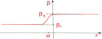
Figure 1: An example of a profile $\,\beta(x)$

A Finite-volume profile states

We shall consider first such states in a finite box $\,[-\frac{1}{4}L,\frac{1}{4}L]\,$ assuming the boundary conditions (2.1) and taking $\,L\,$ sufficiently large so that $\,\beta(x)=\beta_{\cal L}\,$ for $\,x\leq-{\frac{{}_{1}}{{}^{4}}L}\,$ and $\,\beta(x)=\beta_{\cal R}\,$ for $\,x\geq{\frac{{}_{1}}{{}^{4}}L}$.  Let $\,\beta_{L}(x)\,$ be the smooth $\,L$-periodic function on $\,\mathbb{R}\,$ satisfying

$$\beta_{L}(x)\,=\,\begin{cases}\,\beta(x)\hskip 53.20651pt{\rm for}\qquad x\in[-{\frac{1}{4}L},{\frac{1}{4}L}]\hskip 0.71114pt,\cr\,\beta(-x-\frac{1}{2}L)\qquad{\rm for}\qquad x\in[-{\frac{3}{4}L},-{\frac{1}{4}L}]\hskip 0.71114pt,\end{cases}$$ (4.2)

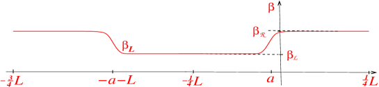
Figure 2: The extended inverse-temperature profile

see Fig. 2. The relations

$$\beta_{L}(x+L)=\beta_{L}(x)\,,\qquad\beta_{L}(-x-\frac{{}_{1}}{{}^{2}}L)=\beta_{L}(x)$$ (4.3)

hold then for all real $\,x$.  Let for the energy density $\,{\cal E}(t,x)\,$ given by (2.6),

$$G_{L}(t)\,=\,\int_{-{\frac{{}_{1}}{{}^{4}}L}}^{{\frac{{}_{1}}{{}^{4}}L}}\beta(x)\,{\cal E}(t,x)\,dx\,=\,v\int_{{\cal I}_{L}}\beta_{L}(x)\,T(x^{-})\,dx\,=\,v\int_{{\cal I}_{L}}\beta_{L}(x^{+})\,T(x)\,dx\,,$$ (4.4)

where we used (2.2) and (4.2) denoting by $\,{\cal I}_{L}\,$ the extended interval $\,[-\frac{3}{4}L,\frac{1}{4}L]$. As will be shown below, $\,G_{L}(t)\,$ is a bounded below self-adjoint operator such that $\,\hbox{Tr}\big{(}{\rm e}^{-G_{L}(t)}\big{)}<\infty$,  see also FH1 .  We shall consider the finite-box nonequilibrium state with expectation values defined by

$$\big{\langle}A\big{\rangle}^{\rm neq}_{L}\,=\,\frac{\hbox{Tr}\,\big{(}A\,{\rm e}^{-G_{L}(0)}\big{)}}{\hbox{Tr}\,\big{(}{\rm e}^{-G_{L}(0)}\big{)}}\hskip 0.71114pt.$$ (4.5)

B Relation between nonequilibrium and equilibrium states

Let $\,h_{L}\,$ be a function on the real line defined by

$$h_{L}(x)\,=\,\beta_{0,L}\int_{-{\frac{{}_{1}}{{}^{4}}L}}^{x}\beta_{L}(x^{\prime})^{-1}dx^{\prime}\,-\,{\frac{{}_{1}}{{}^{4}}L}\qquad\text{for}\qquad\beta_{0,L}^{-1}\,=\,2L^{-1}\int_{-{\frac{{}_{1}}{{}^{4}}L}}^{{\frac{{}_{1}}{{}^{4}}L}}\beta(x)^{-1}dx\hskip 0.71114pt.\ \quad$$ (4.6)

Then

$$h_{L}^{\prime}(x)\ =\,\frac{{}_{\beta_{0,L}}}{{}^{\beta_{L}(x)}},$$ (4.7)

$$h_{L}(x+L)\ =\,\beta_{0,L}\int_{-{\frac{{}_{1}}{{}^{4}}L}}^{x}\beta_{L}(x^{\prime})^{-1}dx^{\prime}+\beta_{0,L}\int_{x}^{x+L}\beta_{L}(x^{\prime})^{-1}dx^{\prime}-{\frac{{}_{1}}{{}^{4}}L}$$ (4.8)

$$\hskip 59.75095pt=\beta_{0,L}\int_{-{\frac{{}_{1}}{{}^{4}}L}}^{x}\beta_{L}(x^{\prime})^{-1}dx^{\prime}+L-\frac{{}_{1}}{{}^{4}}L=h_{L}(x)+L\,,\qquad$$ (4.9)

$$h_{L}(-x-\frac{{}_{1}}{{}^{2}}L)=\beta_{0,L}\int_{-{\frac{{}_{1}}{{}^{4}}L}}^{-x-\frac{{}_{1}}{{}^{2}}L}\beta_{L}(x^{\prime})^{-1}dx^{\prime}-{\frac{{}_{1}}{{}^{4}}L}=\beta_{0,L}\int_{-{\frac{{}_{1}}{{}^{4}}L}}^{-x-\frac{{}_{1}}{{}^{2}}L}\beta_{L}(-x^{\prime}-\frac{{}_{1}}{{}^{2}}L)^{-1}dx^{\prime}-{\frac{{}_{1}}{{}^{4}}L}$$ (4.10)

$$\hskip 59.75095pt=-\beta_{0,L}\int_{-{\frac{{}_{1}}{{}^{4}}L}}^{x}\beta_{L}(x^{\prime})^{-1}dx^{\prime}-{\frac{{}_{1}}{{}^{4}}L}=-h_{L}(x)-\frac{{}_{1}}{{}^{2}}L\,.$$ (4.11)

In particular, $\,h_{L}\in{Diff_{+}{}^{{}^{\sim}}S^{1}}$.  It follows then from (4.4) and the transformation rule (2.11) that

$$U(h_{L})\,G_{L}(t)\,U(h_{L})^{-1}\,=\,v\int_{{\cal I}_{L}}\beta_{L}(x^{+})\,\Big{(}h^{\prime}_{L}(x)^{2}\,T_{+}(h_{L}(x))-\frac{{}_{c}}{{}^{24\pi}}(Sh_{L})(x)\Big{)}dx$$ (4.12)

$$=\,\gamma_{L}\int_{{\cal I}_{L}}\beta_{L}(x^{+})\hskip 0.71114pt\beta_{L}(x)^{-1}T_{+}(h_{L}(x))\,dh_{L}(x)\,-\,C_{t,L}\,=\,\int_{{\cal I}_{L}}\zeta_{t,L}(y)\,T_{+}(y)\,dy\,-\,C_{t,L}\,,$$ (4.13)

where we introduced the notation $\,\gamma_{L}=v\beta_{0,L}\,$ for the combination of dimension of length that will frequently appear below and where

$$C_{t,L}=\frac{{}_{cv}}{{}^{24\pi}}\int_{{\cal I}_{L}}\beta_{L}(x^{+})\,(Sh_{L})(x)\,dx$$ (4.14)

is a number and to obtain the last equality in (4.13) we changed the variable of integration to $\,y=h_{L}(x)\,$ setting

$$\zeta_{t,L}(y)=\gamma_{L}\frac{\beta_{L}(h_{L}^{-1}(y)+vt)}{\beta_{L}(h_{L}^{-1}(y))}\hskip 0.71114pt.$$ (4.15)

Note for the later use that

$$\zeta_{t,L}(y+L)=\zeta_{L,t}(y)\,,\qquad\zeta_{t,L}(-y-\frac{{}_{1}}{{}^{2}}L)=\zeta_{-t,L}(y)\,.$$ (4.16)

Since $\,\zeta_{0,L}(y)=\gamma_{L}$,  it follows, in particular, that

$$U(h_{L})\,G_{L}(0)\,U(h_{L})^{-1} = \beta_{0,L}H_{L}\,-\,C_{0,L}$$ (4.17)

and that $\,G_{L}(0)\,$ is a bounded below self-adjoint operator (and so is $\,G_{L}(t)\,$ because of (2.8)). The identity (4.17) allows to relate the non-equilibrium to equilibrium expectation values:

$$\big{\langle}A\big{\rangle}^{\rm neq}_{L}\,=\,\big{\langle}U(h_{L})\,A\hskip 1.9919ptU(h_{L})^{-1}\big{\rangle}_{\beta_{0,L};L}^{\rm eq}\,.$$ (4.18)

Although essentially tautological, this relation is the main result of the present section. It means that the nonequilibrium state is obtained from the equilibrium one by the composition with the action of a $\,{Diff_{+}{}^{{}^{\sim}}S^{1}}\,$ symmetry on observables. in particular, using (2.11), (2.19) and (2.24), we infer from (4.18) that

$$\Big{\langle}\prod\limits_{i}T_{+}(x_{i})\,\prod\limits_{j}T_{-}(x_{j})\Big{\rangle}^{\rm neq}_{L}$$ (4.19)

$$\,=\,\Big{\langle}\prod\limits_{i}\Big{(}h^{\prime}_{L}(x_{i})^{2}\,T_{+}(h_{L}(x_{i}))-\frac{{}_{c}}{{}^{24\pi}}(Sh_{L})(x_{i})\Big{)}\,\prod\limits_{j}\Big{(}h^{\prime}_{L}(x_{j})^{2}\,T_{-}(h_{L}(x_{j}))-\frac{{}_{c}}{{}^{24\pi}}(Sh_{L})(x_{j})\Big{)}\Big{\rangle}_{\beta_{0,L};L}^{\rm eq},\qquad$$ (4.20)

(4.21)

$$\Big{\langle}\prod\limits_{i}\Phi_{i}(x_{i}^{-},x^{+}_{i})\Big{\rangle}^{\rm neq}_{L}\,=\,\prod\limits_{i}\Big{(}h^{\prime}_{L}(x_{i}^{-})^{\Delta^{+}_{\Phi}}\,h^{\prime}_{L}(x_{i}^{+})^{\Delta^{-}_{\Phi}}\Big{)}\Big{\langle}\prod\limits_{i}\Phi_{+}\big{(}h_{L}(x_{i}^{-}),h_{L}(x_{i}^{+})\big{)}\Big{\rangle}_{\beta_{0,L};L}^{\rm eq}.$$ (4.22)

Analogous relations were obtained in GLM for CFT in a periodic box.

Remark.  Using more general $L$-periodic inverse-temperature profiles $\beta_{L}(x)$ equal to $\beta_{\cal L}$ around $x=-\frac{1}{4}L$ and $\beta_{\cal R}$ around $\frac{1}{4}L$, one may similarly obtain expression for the nonequilibrium expectations with $\,G_{L}(0)\,$ in (4.5) replaced by

$$v\int_{-{\frac{{}_{1}}{{}^{4}}L}}^{{\frac{{}_{1}}{{}^{4}}L}}\big{(}\beta_{+}(x)\,T_{+}(x)+\beta_{-}(x)T_{-}(x)\big{)}\,dx$$ (4.23)

for $\,\beta_{+}(x)=\beta_{L}(x)\,$ and $\,\beta_{-}(x)=\beta_{L}(-x-\frac{{}_{1}}{{}^{2}}L)$,  i.e. for the right- and left-movers corresponding to different temperature profiles with the same asymptotics. The boundary conditions (2.1) do not admit, however, nonequilibrium states corresponding to different profiles $\,\beta_{\pm}(x)\,$ possessing arbitrary asymptotic values that were discussed in GLM using periodic boundary conditions.

C Thermodynamic limit

The thermodynamic limit $\,L\to\infty\,$ of the expectations (4.20) may be controlled similarly as in GLM . First, we observe that, for the fixed inverse-temperature profile (4.1),

$$\beta_{0,L}^{-1}\,=\,2L^{-1}(\Delta\beta^{-1}_{{\cal L}}+\Delta\beta_{\cal R}^{-1})\,+\,\frac{{}_{1}}{{}^{2}}(\beta_{\cal L}^{-1}+\beta_{\cal R}^{-1})\,,$$ (4.24)

where

$$\Delta\beta^{-1}_{\cal L}=\int_{-\infty}^{0}\big{(}\beta(x)^{-1}-\beta_{\cal L}^{-1}\big{)}\,dx\,,\qquad\Delta\beta^{-1}_{\cal R}=\int_{0}^{\infty}\big{(}\beta(x)^{-1}-\beta_{\cal R}^{-1}\big{)}\,dx\,.$$ (4.25)

It follows that

$$\beta_{0,L}\,=\,\frac{{}_{2}}{{}^{\beta_{\cal L}^{-1}+\beta_{\cal R}^{-1}}}-\frac{{}_{8}}{{}^{(\beta_{\cal L}^{-1}+\beta_{\cal R}^{-1})^{2}}}\,(\Delta\beta^{-1}_{\cal L}+\Delta\beta^{-1}_{\cal R})\,L^{-1}\ +\ O(L^{-2})\,,$$ (4.26)

In particular,

$$\lim\limits_{L\to\infty}\,\beta_{0,L}=\frac{{}_{2}}{{}^{\beta_{\cal L}^{-1}+\beta_{\cal R}^{-1}}}\equiv\beta_{0}\,.$$ (4.27)

Similarly, for fixed $\,x$,

$$h_{L}(x)\,=\,\beta_{0,L}\Big{(}\Delta\beta^{-1}_{\cal L}+\frac{{}_{1}}{{}^{4}}\beta_{\cal L}^{-1}{L}\,+\,\int_{0}^{x}\beta(x^{\prime})^{-1}dx^{\prime}\Big{)}\,-\,{\frac{{}_{1}}{{}^{4}}L}$$ (4.28)

$$=\,\frac{{}_{1}}{{}^{4}}\frac{{}_{\beta_{\cal L}^{-1}-\beta_{\cal R}^{-1}}}{{}^{\beta_{\cal L}^{-1}+\beta_{\cal R}^{-1}}}L+\frac{{}_{2(\Delta\beta^{-1}_{\cal L}\beta_{\cal R}^{-1}-\Delta\beta^{-1}_{\cal R}\beta_{{\cal L}}^{-1})}}{{}^{(\beta^{-1}_{\cal L}+\beta_{\cal R}^{-1})^{2}}}+\frac{{}_{2}}{{}^{\beta_{\cal L}^{-1}+\beta_{\cal R}^{-1}}}\int_{0}^{x}\beta(x^{\prime})^{-1}dx^{\prime}\ +\ O(L^{-1})\,.$$ (4.29)

Since $\,\lim\limits_{L\to\infty}\beta_{0,L}=\beta_{0}\,$ and $\,\beta_{L}(x)=\beta(x)\,$ for $\,|x|\leq{\frac{{}_{1}}{{}^{4}}L}$,  it is enough to study the limit of the equilibrium expectations

$$\Big{\langle}\prod\limits_{i}T_{+}(y_{i,L}))\,\prod\limits_{j}T_{-}(y_{j,L})\Big{\rangle}_{\beta_{0,L};L}^{\rm eq}$$ (4.30)

with $\,y_{k,L}=h_{L}(x_{k})\,$ for $\,k=i\,$ or $\,k=j$, and with the products running over subsets of the original indices. The latter equilibrium expectations are the amplitudes of the Euclidean CFT on a cylinder of spatial length $\,L\,$ and temporal circumference $\,\gamma_{L}=v\beta_{0,L}$,  see Fig. 3. In the dual picture interchanging the roles of the space and of the Euclidean time, they may be represented as matrix elements in the theory on the spatial circle of length $\,\gamma_{L}\,$ with the variable $\,\frac{x}{v}\,$ playing the role of the Euclidean time:

Figure 3: Euclidian cylinder

$$\Big{\langle}\prod\limits_{i}T_{+}(y_{i,L})\,\prod\limits_{j}T_{-}(y_{j,L})\Big{\rangle}^{\rm eq}_{\beta_{0,L};L}$$ (4.31)

$$=\,\frac{\big{\langle}\big{\langle}B_{\cal L}\big{|}\big{|}\,{\rm e}^{-{\frac{{}_{1}}{{}^{4v}}L}H_{\gamma_{L}}}\,{\cal T}\big{(}\prod\limits_{i}(-T_{+}(\mathrm{i}y_{i,L}))\prod\limits_{j}(-T_{-}(-\mathrm{i}y_{j,L}))\big{)}\,{\rm e}^{-{\frac{{}_{1}}{{}^{4v}}L}H_{\gamma_{L}}}\big{|}\big{|}B_{\cal R}\big{\rangle}\big{\rangle}}{\big{\langle}\big{\langle}B_{\cal L}\big{|}\big{|}\,{\rm e}^{-\frac{{}_{1}}{{}^{v}}LH_{\gamma_{L}}}\big{|}\big{|}B_{\cal R}\big{\rangle}\big{\rangle}},\quad$$ (4.32)

where $\,\big{|}\big{|}B_{\cal L}\big{\rangle}\big{\rangle}\,$ and $\,\big{|}\big{|}B_{\cal R}\big{\rangle}\big{\rangle}\,$ are the states in the (extended) space of states of the theory on the circle of circumference $\,\gamma_{L}\,$ (an appropriate combinations of the so-called Ishibashi states Ishi ) that represent the conformal boundary conditions at the ends of the interval $[-{\frac{{}_{1}}{{}^{4}}L},{\frac{{}_{1}}{{}^{4}}L}]$,  the operator $\,H_{\gamma_{L}}\,$ is the Hamiltonian of that theory,

$$T_{\pm}(x\pm\mathrm{i}v\tau)\,=\,{\rm e}^{\tau H_{\gamma_{L}}}T_{\pm}(x)\,{\rm e}^{-\tau H_{\gamma_{L}}}\,,$$ (4.33)

with $\,T_{\pm}(x)\,$ standing for the components of the energy-momentum tensor of the theory on the circle,  see Appendix A,  and $\,{\cal T}\,$ reorders the factors so that $\,y_{i,L}\,$ and $\,y_{j,L}\,$ increase from right to left.

This type of finite-volume equilibrium expectations is standard in CFT Cardy and was discussed in detail for the compactified free massless field in Gab or GT . In that case, the dual theory on the circle of length $\,\gamma_{L}\,$ used in the representation (4.32) has the field with the periodic boundary condition $\,\varphi(t,x)=\varphi(t,x+\gamma_{L})\,$ leading to independent left- and right-moving components and two commuting sets of modes $\,\alpha_{n}\,$ and $\,\bar{\alpha}_{n}\,$ satisfying each the relations (3.10). The zero-mode space is generated by orthonormal vectors $\,|k,w\rangle\,$ with $\,k,w\in\mathbb{Z}$, $\,k\,$ corresponding to the momentum and $\,w\,$ the winding number of the fields.  One has

$$\frac{{}_{r}}{{}^{\sqrt{2}}}(\alpha_{0}+\bar{\alpha}_{0})|k,w\rangle=k|k,w\rangle\,,\quad\frac{{}_{1}}{{}^{\sqrt{2}r}}(\alpha_{0}-\bar{\alpha}_{0})|k,w\rangle=w|k,w\rangle\,,\quad\alpha_{n}|k,w\rangle=0=\bar{\alpha}_{n}|k,w\rangle\ \,{\rm for}\ \,n>0.\qquad\ \$$ (4.34)

The dual-theory boundary states representing the Neumann boundary conditions (3.9) of the original theory have the form Polch

$$\big{|}\big{|}B_{{\cal L}}\big{\rangle}\big{\rangle}\,=\,{\rm e}^{-\sum\limits_{n=1}^{\infty}\frac{1}{n}\hskip 0.56917pt\alpha_{-n}\bar{\alpha}_{-n}}\sum\limits_{w\in\mathbb{Z}}|0,w\rangle\,=\,\big{|}\big{|}B_{{\cal R}}\big{\rangle}\big{\rangle}.$$ (4.35)

The action of $\,\alpha_{-n}\,$ or $\,\bar{\alpha}_{-n}\,$ for $\,n>0\,$ raises the eigenvalue of the Hamiltonian $\,H_{\gamma_{L}}\,$ of the theory by $\,\frac{2\pi n}{\beta_{0,L}}\,$ whereas $\,H_{\gamma_{L}}|k,w\rangle=\frac{\pi}{\beta_{0,L}}(r^{-2}k^{2}+r^{2}w^{2}-\frac{{}_{1}}{{}^{6}})$.  The vacuum vector is $\,|0,0\rangle$.

Coming back to the general case, let

$$\widetilde{y}_{k,L}=h_{L}(x_{k})-\frac{{}_{1}}{{}^{4}}\frac{{}_{\beta_{\cal L}^{-1}-\beta_{\cal R}^{-1}}}{{}^{\beta_{\cal L}^{-1}+\beta_{\cal R}^{-1}}}L$$ (4.36)

so that

$$\lim\limits_{L\to\infty}\,\widetilde{y}_{k,L}=y_{0}+h(x_{k})$$ (4.37)

for $\,y_{0}\equiv\frac{{2(\Delta\beta^{-1}_{\cal L}\beta_{\cal R}^{-1}-\Delta\beta^{-1}_{\cal R}\beta_{{\cal L}}^{-1})}}{{(\beta^{-1}_{\cal L}+\beta_{\cal R}^{-1})^{2}}}\,$ and

$$h(x)=\int_{0}^{x}\frac{{}_{\beta_{0}}}{{}^{\beta(x^{\prime})}}\,dx^{\prime}\hskip 0.71114pt.$$ (4.38)

Note that

$$\frac{{}_{1}}{{}^{4}}L-\frac{{}_{1}}{{}^{4}}\frac{{}_{\beta_{\cal L}^{-1}-\beta_{\cal R}^{-1}}}{{}^{\beta_{\cal L}^{-1}+\beta_{\cal R}^{-1}}}L=\frac{{}_{\beta_{\cal R}^{-1}}}{{}^{2(\beta_{\cal L}^{-1}+\beta_{\cal R}^{-1})}}L\,,\qquad\frac{{}_{1}}{{}^{4}}L+\frac{{}_{1}}{{}^{4}}\frac{{}_{\beta_{\cal L}^{-1}-\beta_{\cal R}^{-1}}}{{}^{\beta_{\cal L}^{-1}+\beta_{\cal R}^{-1}}}L=\frac{{}_{\beta_{\cal L}^{-1}}}{{}^{2(\beta_{\cal L}^{-1}+\beta_{\cal R}^{-1})}}L\hskip 0.71114pt.$$ (4.39)

If we replace $\,\beta_{0,L}\,$ by its limiting value $\,\beta_{0}\,$ on the right-hand side of (4.32) and denote $\,v\beta_{0}=\gamma\,$ then

$$\frac{{\big{\langle}\big{\langle}B_{\cal L}\big{|}\big{|}\,{\rm e}^{-{\frac{{}_{1}}{{}^{4v}}L}H_{\gamma}}\,{\cal T}\Big{(}\prod\limits_{i}(-T_{+}(\mathrm{i}y_{i,L}))\prod\limits_{j}(-T_{-}(-\mathrm{i}y_{j,L}))\Big{)}\,{\rm e}^{-{\frac{{}_{1}}{{}^{4v}}L}H_{\gamma}}\big{|}\big{|}B_{\cal R}\big{\rangle}\big{\rangle}}}{{\big{\langle}\big{\langle}B_{\cal L}\big{|}\big{|}\,{\rm e}^{-\frac{{}_{1}}{{}^{2v}}LH_{\gamma}}\big{|}\big{|}B_{\cal R}\big{\rangle}\big{\rangle}}}$$ (4.40)

$$=\,\frac{{\big{\langle}\big{\langle}B_{\cal L}\big{|}\big{|}\,{\rm e}^{-\frac{{}_{\beta_{\cal R}^{-1}}}{{}^{2(\beta_{\cal L}^{-1}+\beta_{\cal R}^{-1})v}}LH_{\gamma}}\,{\cal T}\Big{(}\prod\limits_{i}(-T_{+}(\mathrm{i}\widetilde{y}_{i,L}))\prod\limits_{j}(-T_{-}(-\mathrm{i}\widetilde{y}_{j,L}))\Big{)}\,\hskip 0.71114pt{\rm e}^{-\frac{{}_{\beta_{\cal L}^{-1}}}{{}^{2(\beta_{\cal L}^{-1}+\beta_{\cal R}^{-1})v}}LH_{\gamma}}\big{|}\big{|}B_{\cal R}\big{\rangle}\big{\rangle}}}{{\big{\langle}\big{\langle}B_{\cal L}\big{|}{\rm e}^{-\frac{{}_{1}}{{}^{2v}}LH_{\gamma}}\big{|}\big{|}B_{\cal R}\big{\rangle}\big{\rangle}}}$$ (4.41)

(4.42)

(4.43)

$$\mathop{\longrightarrow}\limits_{L\to\infty}\ \big{\langle}0\big{|}\,{\cal T}\Big{(}\prod\limits_{i}(-T_{+}(\mathrm{i}(y_{0}+y_{i})))\prod\limits_{j}(-T_{-}(-\mathrm{i}(y_{0}+y_{j})))\Big{)}\big{|}0\big{\rangle}$$ (4.44)

(4.45)

$$\hskip 28.45274pt=\,\big{\langle}0\big{|}\,{\cal T}\Big{(}\prod\limits_{i}(-T_{+}(\mathrm{i}y_{i}))\prod\limits_{j}(-T_{-}(-\mathrm{i}y_{j}))\Big{)}\big{|}0\big{\rangle}\ =\ \Big{\langle}\prod\limits_{i}T_{+}(y_{i})\prod\limits_{j}T_{-}(y_{j})\Big{\rangle}^{\rm eq}_{\beta_{0}},$$ (4.46)

where $\,y_{k}=h(x_{k})\,$ for $\,k=i\,$ or $\,k=j\,$ and the expectation on the right-hand side is in the infinite-volume Gibbs state at inverse temperature $\,\beta_{0}$.  The limit was obtained using the fact that the leading contribution to $\,{\rm e}^{-CL\hskip 0.71114ptH_{\gamma}}\big{|}\big{|}B_{{\cal L},{\cal R}}\big{\rangle}\big{\rangle}\,$ for $\,C>0\,$ and large $\,L\,$ comes from the vacuum vector $\,\big{|}0\big{\rangle}\,$ of the theory on the circle of radius $\,\gamma$,  with the other contributions exponentially suppressed.  Finally, $\,\beta_{0,L}\,$ on the right hand side of (4.32) may be turned to $\,\beta_{0}\,$ by rescaling the Euclidian space coordinates by $\,C_{L}\equiv\gamma/\gamma_{L}=1+O(L^{-1})$.  Upon such a rescaling, the theory on the circle of length $\,\gamma_{L}\,$ is mapped to the one on the circle of length $\,\gamma$, $\,T_{\pm}(\pm\mathrm{i}y_{i,L})\,$ to $\,C_{L}^{2}T_{\pm}(\pm\mathrm{i}C_{L}y_{i,L})$, and the boundary states $\,\big{|}\big{|}B_{{\cal L},{\cal R}}\big{\rangle}\big{\rangle}\,$ to states with the similar asymptotic behavior under the action of $\,{\rm e}^{-CL\hskip 0.71114ptH_{\gamma}}\,$ and the argument goes as before. Dropping the subscript $L$ in the infinite-volume limit of the equilibrium and nonequilibrium expectations, we obtain from (4.20) the identity

$$\Big{\langle}\prod\limits_{i}T_{+}(x_{i})\,\prod\limits_{j}T_{-}(x_{j})\Big{\rangle}^{\rm neq}$$ (4.47)

$$\,=\,\Big{\langle}\prod\limits_{i}\big{(}h^{\prime}(x_{i})^{2}\,T_{+}(h(x_{i}))-\frac{{}_{c}}{{}^{24\pi}}(Sh)(x_{i})\big{)}\,\prod\limits_{j}\big{(}h^{\prime}(x_{j})^{2}\,T_{-}(h(x_{j}))-\frac{{}_{c}}{{}^{24\pi}}(Sh)(x_{j})\big{)}\Big{\rangle}^{\rm eq}_{\beta_{0}}\hskip 0.71114pt,\qquad$$ (4.48)

where $\,\beta_{0}\,$ and $\,h\,$ are given by (4.27) and (4.38). This is the same infinite-volume relation that was obtained in GLM using in finite volume the periodic boundary conditions. In particular, one gets

$$\Big{\langle}T_{\pm}(x)\Big{\rangle}^{\rm neq}=\frac{{\pi c}}{{12(v\beta(x))^{2}}}-\frac{c}{{24\pi}}(Sh)(x)\,.$$ (4.49)

$$\Big{\langle}T_{\pm}(x_{1})\,;\,T_{\pm}(x_{2})\Big{\rangle}^{{\rm neq},\,c}\,=\,\frac{{\pi^{2}c}}{8(v\beta(x_{1}))^{2}(v\beta(x_{2}))^{2}\sinh^{4}\big{(}\frac{\pi}{\gamma}(h(x_{1})-h(x_{2})\big{)}}\,,$$ (4.50)

$$\Big{\langle}T_{\pm}(x_{1})\,;\,T_{\mp}(x_{2})\Big{\rangle}^{{\rm neq},\,c}\,=\,0\,,$$ (4.51)

where $\,\big{\langle}\ \,;\ \big{\rangle}^{{\rm neq},\,c}$ denotes the infinite-volume limit of the connected expectations.

For (4.22), the thermodynamic limit reduces again to that for the equilibrium expectation values. For the equal-time correlations or if the primary fields are chiral, the latter may be controlled the same way as above. For non-chiral fields at non-equal times, one should first analytically continue to imaginary times. For Euclidian points with purely imaginary times the thermodynamic limit may again be controlled by passing to the dual picture that leads to the vacuum expectation values. This should yield the convergence for $\,L\to\infty\,$ of the analytic continuations to imaginary times of the equilibrium correlators of the primary fields and, in turn, of their boundary values with real times. The thermodynamic limit of the latter may also be controlled directly for the examples of CFTs and their primary fields discussed above. The end result is the infinite-volume version

$$\Big{\langle}\prod\limits_{i}\Phi_{i}(x_{i}^{-},x^{+}_{i})\Big{\rangle}^{\rm neq}\,=\,\prod\limits_{i}\Big{(}h^{\prime}(x_{i}^{-})^{\Delta^{+}_{\Phi}}\,h^{\prime}(x_{i}^{+})^{\Delta^{-}_{\Phi}}\Big{)}\Big{\langle}\prod\limits_{i}\Phi_{+}(h(x_{i}^{-}),h(x_{i}^{+}))\Big{\rangle}^{\rm eq}_{\beta_{0}}$$ (4.52)

of the identity (4.22) GLM .

Remark.  The condition $\,\beta_{0}=\frac{2}{\beta_{\cal L}^{-1}+\beta_{\cal R}^{-1}}\,$ in (4.38), (4.48) and (4.52) may be dropped using the scaling properties of the infinite-volume equilibrium state.

5 Full counting statistics of energy transfers:  preliminaries

A Two-time measurement protocol

The aim of the subsequent part of the paper is to describe the statistics of energy transfers in the nonequilibrium states with preimposed inverse-temperature profile with a kink as in Fig. 1. To access that statistics, we shall follow a two-time quantum measurement protocol [LL, ,MA, ,BD0, ]. To this end, we consider in the setup of Sec. 4 the observables

$$G_{L}(t)\,=\,{\rm e}^{\mathrm{i}tH_{L}}\,G_{L}(0)\hskip 0.71114pt\,{\rm e}^{-\mathrm{i}tH_{L}}$$ (5.1)

defined by (4.4) and possessing the spectral decompositions

$$G_{L}(t)\,=\,\sum\limits_{i}g_{i}\hskip 0.71114ptP_{i,L}(t)$$ (5.2)

with $\,P_{i,L}(t)={\rm e}^{\mathrm{i}tH_{L}}P_{i,L}(0)\,{\rm e}^{-\mathrm{i}tH_{L}}$.  If the inverse-temperature profile $\,\beta(x)\,$ is a narrow kink with constant values $\,\beta_{\cal L}\,$ and $\,\beta_{\cal R}\,$ to the left and to the right, respectively, of a small interval $\,[a-\delta,a+\delta]\,$ then

$$G_{L}(t)=\beta_{\cal L}E_{\cal L}(t)+\beta_{\cal R}E_{\cal R}(t)\,,$$ (5.3)

where the observable $\,E_{\cal L}(t)\,$ measures the energy in the system at time $\,t\,$ to the left of the kink and $\,E_{\cal R}(t)\,$ the one to the right of the kink (redistributing the small energy contained within the kink appropriately).

Suppose that we measure the observable $\,G_{L}(0)\,$ in the nonequilibrium state $\,\omega^{\rm neq}_{L}\,$ given by (4.5). The probability to obtain the result $\,g_{i}\,$ is

$$p_{L}(g_{i})\,=\,\big{\langle}P_{i,L}(0)\big{\rangle}^{\rm neq}_{L}=\frac{\hbox{Tr}\,\big{(}P_{i,L}(0)\,{\rm e}^{-G_{L}(0)}\big{)}}{\hbox{Tr}\,\big{(}{\rm e}^{-G_{L}(0)}\big{)}}$$ (5.4)

and, after the measurement,  the nonequilibrium state is reduced to the new state with expectations

$$\big{\langle}A\big{\rangle}_{i,L}\,=\,\frac{\hbox{Tr}\,\big{(}P_{i,L}(0)\,A\,P_{i,L}(0)\,{\rm e}^{-G_{L}(0)}\big{)}}{\hbox{Tr}\,\big{(}P_{i,L}(0)\,{\rm e}^{-G_{L}(0)}\big{)}}\,=\,\frac{\hbox{Tr}\,\big{(}A\,P_{i,L}(0)\,{\rm e}^{-G_{L}(0)}\big{)}}{\hbox{Tr}\,\big{(}P_{i,L}(0)\,{\rm e}^{-G_{L}(0)}\big{)}}\,,$$ (5.5)

where the second equality follows from the commutation of $\,P_{i,L}(0)\,$ with $\,G_{L}(0)$.  We now let this state evolve for time $\,t\,$ and then measure the observable $\,G_{L}(0)\,$ for the second time. This is equivalent to the measurement of the observable $\,G_{L}(t)\,$ in the state with expectations given by (5.5).  The probability that the result of the second measurement is $\,g_{j}$, under the condition that the first one was $\,g_{i}$,  is then equal to

$$p_{t,L}(g_{j}|\,g_{i})\,=\,\big{\langle}P_{j,L}(t)\big{\rangle}_{i,L}\,=\,\frac{\hbox{Tr}\,\big{(}P_{j,L}(t)\hskip 0.71114ptP_{i,L}(0)\,{\rm e}^{-G_{L}(0)}\big{)}}{\hbox{Tr}\,\big{(}P_{i,L}(0)\,{\rm e}^{-G_{L}(0)}\big{)}}\,.$$ (5.6)

Hence the probability to get the results $\,(g_{i},g_{j})\,$ in the two-time measurement of $\,G_{L}(0)\,$ separated by time $\,t\,$ in the nonequilibrium state with expectation values (4.5) is

$$p_{t,L}(g_{i},g_{j})\,=\,p_{L}(g_{i})\,p_{t,L}(g_{i}|g_{j})\,=\,\frac{\hbox{Tr}\,\big{(}P_{j,L}(t)\hskip 0.71114ptP_{i,L}(0)\,{\rm e}^{-G_{L}(0)}\big{)}}{\hbox{Tr}\,\big{(}{\rm e}^{-G_{L}(0)}\big{)}}\,=\,\big{\langle}P_{j,L}(t)\hskip 0.71114ptP_{i,L}(0)\big{\rangle}^{\rm neq}_{L}\,.$$ (5.7)

B The generating function for FCS of energy transfers

We shall consider

$$\Delta E=\frac{g_{j}-g_{i}}{\Delta\beta}\,,$$ (5.8)

where $\,\Delta\beta\equiv\beta_{\cal R}-\beta_{\cal L}$,  as a measure of the net energy transfer through the kink during time $\,t$.  Indeed, the energy on the right of the kink should change in time $\,t\,$ by $\,\Delta E\,$ and on the left of the kink by $\,-\Delta E\,$ so that, by (5.3), $\,g_{j}-g_{i}\,$ should be equal to $\,\beta_{\cal R}\Delta E-\beta_{\cal L}\Delta E$. Upon the identification (5.8), the PDF of $\,\Delta E$,  called Full Counting Statistics (FCS) QN of energy transfers,  takes the form

$$P_{t,L}(\Delta E)\,=\,\sum\limits_{i,j}\,\delta\Big{(}\Delta E-\frac{g_{j}-g_{i}}{\Delta\beta}\Big{)}\,p_{t,L}(g_{i},g_{j})$$ (5.9)

and its Fourier transform (called the FCS generating function) becomes

$$\Psi_{t,L}(\lambda) = \int{\rm e}^{\mathrm{i}\lambda\Delta E}\,P_{t,L}(\Delta E)\,\,d(\Delta E)\,=\,\sum\limits_{i,j}{\rm e}^{\frac{\mathrm{i}\lambda(g_{j}-g_{i})}{\Delta\beta}}\,p_{t,L}(g_{i},g_{j})$$ (5.10)

$$= \sum\limits_{i,j}{\rm e}^{\frac{\mathrm{i}\lambda(g_{j}-g_{i})}{\Delta\beta}}\,\big{\langle}P_{j,L}(t)\hskip 0.71114ptP_{i,L}(0)\big{\rangle}^{\rm neq}_{L}\,=\,\big{\langle}{\rm e}^{\frac{\mathrm{i}\lambda}{\Delta\beta}G_{L}(t)}\,{\rm e}^{-\frac{\mathrm{i}\lambda}{\Delta\beta}G_{L}(0)}\big{\rangle}^{\rm neq}_{L}\,.$$ (5.11)

In particular, the average of the energy transfer

$$\langle\Delta E\rangle_{t,L}\,=\,\frac{{}_{1}}{{}^{\mathrm{i}}}\,\partial_{\lambda}\ln{\Psi_{t,L}(0)}\,=\,(\Delta\beta)^{-1}\,\big{\langle}G_{L}(t)-G_{L}(0)\big{\rangle}^{\rm neq}_{L}$$ (5.12)

and its variance

$$\langle\Delta E;\Delta E\rangle^{c}_{t,L}\,=\,-\partial_{\lambda}^{2}\hskip 0.71114pt\ln{\Psi_{t,L}(0)}\,=\,(\Delta\beta)^{-2}\,\big{\langle}G_{L}(t)-G_{L}(0);G_{L}(t)-G_{L}(0)\big{\rangle}^{{\rm neq},\,c}_{L}\,.$$ (5.13)

$\,\Psi_{t,L}(\lambda)\,$ extends to an analytic function in the interior of the strip $\,0\leq{\rm Im}(\lambda)\leq\Delta\beta\,$ if $\,\Delta\beta>0\,$ and $\,\Delta\beta\leq{\rm Im}(\lambda)\leq 0\,$ if $\,\Delta\beta<0$,  with the boundary value

$$\Psi_{t,L}(-\lambda+\mathrm{i}\Delta\beta) = \frac{\hbox{Tr}\,\big{(}{\rm e}^{-\frac{\mathrm{i}\lambda+\Delta\beta}{\Delta\beta}G_{L}(t)}\,{\rm e}^{\frac{\mathrm{i}\lambda+\Delta\beta}{\Delta\beta}G_{L}(0)}\,{\rm e}^{-G_{L}(0)}\big{)}}{\hbox{Tr}\,\big{(}{\rm e}^{-G_{L}(0)}\big{)}}\,=\,\frac{\hbox{Tr}\,\big{(}{\rm e}^{-G_{L}(t)}{\rm e}^{-\frac{\mathrm{i}\lambda}{\Delta\beta}G_{L}(t)}{\rm e}^{\frac{\mathrm{i}\lambda}{\Delta\beta}G_{L}(0)}\big{)}}{\hbox{Tr}\,\big{(}{\rm e}^{-G_{L}(0)}\big{)}}$$ (5.15)

$$=\,\frac{\hbox{Tr}\,\big{(}{\rm e}^{-G_{L}(0)}{\rm e}^{-\frac{\mathrm{i}\lambda}{\Delta\beta}G_{L}(0)}{\rm e}^{\frac{\mathrm{i}\lambda}{\Delta\beta}G_{L}(-t)}\big{)}}{\hbox{Tr}\,\big{(}{\rm e}^{-G_{L}(0)}\big{)}}\,=\,\frac{\hbox{Tr}\,\big{(}{\rm e}^{\frac{\mathrm{i}\lambda}{\Delta\beta}G_{L}(-t)}\,{\rm e}^{-\frac{\mathrm{i}\lambda}{\Delta\beta}G_{L}(0)}\,{\rm e}^{-G_{L}(0)}\big{)}}{\hbox{Tr}\,\big{(}{\rm e}^{-G_{L}(0)}\big{)}}\,=\,\Psi_{-t,L}(\lambda)\,.\qquad$$

The above identity is a “fluctuation relation” between the FCS generating functions for the direct and the time reversed dynamics. If the CFT is time-reversal invariant so that there exists an anti-unitary involution or anti-involution $\,\Theta\,$ such that $\,\Theta\hskip 0.28436ptT_{\pm}(x)\Theta^{-1}=T_{\mp}(x)\,$ and,  consequently, $\,\Theta\hskip 0.85355ptG_{L}(t)\Theta^{-1}=G_{L}(-t)\,$ then

$$\Psi_{-t,L}(\lambda) = \frac{\hbox{Tr}\,\big{(}\Theta\hskip 1.42271pt{\rm e}^{-\frac{\mathrm{i}\lambda}{\Delta\beta}G_{L}(t)}\,{\rm e}^{\frac{\mathrm{i}\lambda}{\Delta\beta}G_{L}(0)}\,{\rm e}^{-G_{L}(0)}\,\Theta^{-1}\big{)}}{\hbox{Tr}\,\big{(}{\rm e}^{-G_{L}(0)}\big{)}}\,=\,\frac{\overline{\hbox{Tr}\,\big{(}{\rm e}^{-\frac{\mathrm{i}\lambda}{\Delta\beta}G_{L}(t)}\,{\rm e}^{\frac{\mathrm{i}\lambda}{\Delta\beta}G_{L}(0)}\,{\rm e}^{-G_{L}(0)}\big{)}}}{\hbox{Tr}\,\big{(}{\rm e}^{-G_{L}(0)}\big{)}}$$ (5.16)

$$= \frac{\hbox{Tr}\,\big{(}{\rm e}^{-\frac{\mathrm{i}\lambda}{\Delta\beta}G_{L}(t)}\,{\rm e}^{\frac{\mathrm{i}\lambda}{\Delta\beta}G_{L}(0)}\,{\rm e}^{-G_{L}(0)}\big{)}^{\dagger}}{\hbox{Tr}\,\big{(}{\rm e}^{-G_{L}(0)}\big{)}}\,=\,\frac{\hbox{Tr}\,\big{(}{\rm e}^{-G_{L}(0)}\,{\rm e}^{-\frac{\mathrm{i}\lambda}{\Delta\beta}G_{L}(0)}\,{\rm e}^{\frac{\mathrm{i}\lambda}{\Delta\beta}G_{L}(t)}\big{)}}{\hbox{Tr}\,\big{(}{\rm e}^{-G_{L}(0)}\big{)}}$$ (5.17)

$$= \frac{\hbox{Tr}\,\big{(}{\rm e}^{\frac{\mathrm{i}\lambda}{\Delta\beta}G_{L}(t)}\,{\rm e}^{-\frac{\mathrm{i}\lambda}{\Delta\beta}G_{L}(0)}\,{\rm e}^{-G_{L}(0)}\big{)}}{\hbox{Tr}\,\big{(}{\rm e}^{-G_{L}(0)}\big{)}}\,=\,\Psi_{t,L}(\lambda)$$ (5.18)

and we infer the “transient” fluctuation relation for the generating function $\,\Psi_{t,L}(\lambda)\,$ [ES, ,Kur, ,BD1, ]:

$$\Psi_{t,L}(\lambda)\,=\,\Psi_{t,L}(-\lambda+\mathrm{i}\Delta\beta)$$ (5.19)

In fact, in the Hilbert of the boundary theory such that $\,T_{+}(x^{-})=T_{-}(x^{+})\,$ for $\,x=\pm\frac{1}{2}L$,  there always exists an anti-unitary involution $\,\Theta\,$ that does the job:  it is sufficient to take $\,\Theta\,$ that preserves the highest-weight vectors of the unitary irreducible representations of the Virasoro algebra and that commutes with the Virasoro generators $\,L_{n}$.  Hence the transient fluctuation relation is always valid in our case.

6 FCS  in finite volume and conformal welding

A FCS  and $\,{Diff_{+}{}^{{}^{\sim}}S^{1}}\,$ characters

Using the relation (4.18) between the nonequilibrium and equilibrium expectations and the transformation identity (4.13), we may rewrite the expression (5.11) for the generating function for FCS of energy transfers in the form

$$\Psi_{t,L}(\lambda) = \big{\langle}U(h_{L})\,\hskip 0.71114pt{\rm e}^{\frac{\mathrm{i}\lambda}{\Delta\beta}G_{L}(t)}\,{\rm e}^{-\frac{\mathrm{i}\lambda}{\Delta\beta}G_{L}(0)}\hskip 0.85355ptU(h_{L})^{-1}\big{\rangle}^{\rm eq}_{\beta_{0,L};L}$$ (6.1)

$$= \big{\langle}{\rm e}^{\frac{\mathrm{i}\lambda}{\Delta\beta}\int_{{}_{{\cal I}_{L}}}\zeta_{t,L}(y)\,T(y)\,dy}\,{\rm e}^{-\frac{\mathrm{i}\lambda}{\Delta\beta}\beta_{0,L}H_{L}}\,\big{\rangle}^{\rm eq}_{\beta_{0,L};L}\,{\rm e}^{-\frac{\mathrm{i}\lambda}{\Delta\beta}(C_{t,L}-C_{0,L})}.$$ (6.3)

In virtue of  (2.7) and (2.15),

$$\big{\langle}{\rm e}^{\frac{\mathrm{i}\lambda}{\Delta\beta}\int_{{}_{{\cal I}_{L}}}\zeta_{t,L}(y)\,T(y)\,dy}\,{\rm e}^{-\frac{\mathrm{i}\lambda}{\Delta\beta}\beta_{0,L}H_{L}}\big{\rangle}^{\rm eq}_{\beta_{0,L};L}$$ (6.4)

$$=\frac{\hbox{Tr}\,\big{(}{\rm e}^{\mathrm{i}\frac{\lambda}{\Delta\beta}\int_{{}_{{\cal I}_{L}}}\zeta_{t,L}(y)\,T(y)\,dy}\,{\rm e}^{-\frac{2\pi\gamma_{L}}{L}(1+\mathrm{i}\frac{\lambda}{\Delta\beta})(L_{0}-\frac{c}{24})}\big{)}}{\hbox{Tr}\,\big{(}{\rm e}^{-\frac{2\pi\gamma_{L}}{L}(L_{0}-\frac{c}{24})}\big{)}}\,=\,\frac{\hbox{Tr}\,\big{(}U(f_{s,t,L})\,\hskip 0.71114pt{\rm e}^{2\pi\mathrm{i}\tau_{s,L}(L_{0}-\frac{c}{24})}\big{)}}{c_{s,\zeta_{t,L}}\,\hbox{Tr}\,\big{(}{\rm e}^{2\pi\mathrm{i}\tau_{0,L}(L_{0}-\frac{c}{24})}\big{)}}$$ (6.5)

where, as before, $\,\gamma_{L}=v\beta_{0,L}\,$ and

$$s=\frac{{}_{\lambda}}{{}^{\Delta\beta}}\,,\qquad\tau_{s,L}=L^{-1}(\mathrm{i}-s)\gamma_{L}$$ (6.6)

and $\,f_{s,t,L}\in{Diff_{+}{}^{{}^{\sim}}S^{1}}\,$ describe the flow of the vector field $\,-\zeta_{t,L}(y)\partial_{y}$.  Note that the relation (4.16) implies that

$$f_{s,t,L}(-y-\frac{{}_{1}}{{}^{2}}L)=-f_{-s,-t,L}(y)-\frac{{}_{1}}{{}^{2}}L\,.$$ (6.7)

The function

$$\chi(\tau)\,=\,\hbox{Tr}\big{(}{\rm e}^{2\pi\mathrm{i}\tau(L_{0}-\frac{c}{24})}\big{)}$$ (6.8)

of $\,\tau\,$ from the complex upper half-plane $\,\mathbb{H}_{+}$,  where the trace is over the space of a Virasoro algebra representation,  defines the character of the latter. Such characters are explicitly known for the (direct sums of) irreducible highest-weight representations of the Virasoro algebra RC . By analogy, we shall call the function

$$\Upsilon(f,\tau)\,=\,\hbox{Tr}\big{(}U(f)\,{\rm e}^{2\pi\mathrm{i}\tau(L_{0}-\frac{c}{24})}\big{)}$$ (6.9)

of $\,f\in{Diff_{+}{}^{{}^{\sim}}S^{1}}\,$ and $\,\tau\in\mathbb{H}_{+}\,$ the character of the projective representation $\,U\,$ of $\,{Diff_{+}{}^{{}^{\sim}}S^{1}}$.  We may then rewrite the relation (6.3) as

$$\Psi_{t,L}(\lambda)\,=\,\frac{\Upsilon(f_{s,t,L}\hskip 0.71114pt,\tau_{s,L})}{c_{s,\zeta_{t,L}}\,\chi(\tau_{0,L})}\,\,{\rm e}^{-\mathrm{i}s\hskip 0.71114pt(C_{t,L}-C_{0,L})}\,,$$ (6.10)

where the characters pertain to the representation of the Virasoro algebra in the space $\,{\cal H}_{L}\,$ of states of the boundary CFT and to its corresponding lift to $\,{Diff_{+}{}^{{}^{\sim}}S^{1}}$.

Unlike the Virasoro characters, the characters $\,\Upsilon(f,\tau)\,$ where not studied in detail and we shall try to fill this gap in the next section for the special case that occurs on the right hand side of (6.10) for which $\,f=f_{s}\,$ belongs to the flow of a vector field.

B Reduction of $\,{Diff_{+}{}^{{}^{\sim}}S^{1}}\,$ characters to Virasoro ones

The Virasoro character $\,\chi(\tau)\,$ of (6.8) is given by the trace of the operator $\,{\rm e}^{2\pi\mathrm{i}\tau(L_{0}-\frac{c}{24})}$.  If $\,\tau\,$ were real, such an operator would represent (up to a phase) a translation in the Cartan subgroup of $\,{Diff_{+}{}^{{}^{\sim}}S^{1}}$,  see (2.16). Instead, $\,\tau\,$ is taken with a positive imaginary part in order to assure the convergence of the trace. In the simpler context of finite-dimensional representations of compact groups, it is enough to know the characters on the Cartan subgroup,  as they are class functions that are constant on conjugacy classes and each conjugacy class contains an element in the Cartan subgroup. When dealing with the characters $\,\Upsilon(f,\tau)\,$ of $\,{Diff_{+}{}^{{}^{\sim}}S^{1}}$,  however,  there are complications. The first one is due to the insertion of the operator $\,{\rm e}^{2\pi\mathrm{i}\tau(L_{0}-\frac{c}{24})}\,$ that represents an element in the complexification of the Cartan subgroup of $\,{Diff_{+}{}^{{}^{\sim}}S^{1}}\,$ and assures the convergence of the trace. The second complication is due to the projectivity of the representation of $\,{Diff_{+}{}^{{}^{\sim}}S^{1}}$. Finally, the conjugacy classes in $\,{Diff_{+}{}^{{}^{\sim}}S^{1}}\,$ rarely contain elements in the Cartan subgroup. All these difficulties find an elegant resolution in the setup advocated by G. Segal Segal where one replaces $\,{Diff_{+}S^{1}}\,$ by a semigroup of complex annuli with parameterized boundaries and one studies its projective representations. Within this approach, the operator $\,U(f)\,{\rm e}^{2\pi\mathrm{i}\tau(L_{0}-\frac{c}{24})}\,$ is proportional to the trace-class operator (the chiral amplitude) representing the complex annulus

$${\cal A}_{f,\tau}=\big{\{}z\in\mathbb{C}\,\big{|}\,|q|\leq|z|\leq 1\big{\}}$$ (6.11)

for $\,q={\rm e}^{2\pi\mathrm{i}\tau}\,$ with the boundary components parameterized by

$$p_{1}(x)=q\,{\rm e}^{-\frac{2\pi\mathrm{i}}{L}f(x)}=p_{1}(x+L)\,,\qquad p_{2}(x)={\rm e}^{-\frac{2\pi\mathrm{i}}{L}x}=p_{2}(x+L)\,,$$ (6.12)

see Fig. 4. The precise normalization of the chiral amplitudes that allows to handle the projectivity of the representations of the semigroup of annuli is fixed in Segal using the theory of determinant line bundles for Riemann surfaces with boundary and we shall not dwell on it here. Within Segal’s approach, the counterpart of the “class-function”property of the compact-group characters is the fact that the trace of the chiral amplitude associated to a complex annulus depends, up to a controllable factor, only on the complex torus obtained from the annulus by “conformal welding” that identifies the two boundary components using their parameterizations. The complex structure of such a welded torus is fixed by defining the local holomorphic functions on it as those whose pullback to the annulus is smooth and holomorphic in the interior.

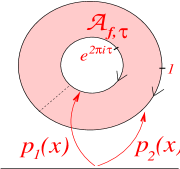
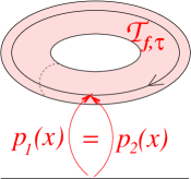
Figure 4: Annulus $\,{\cal A}_{f,\tau}\,$ and torus $\,{\cal T}_{f,\tau}$

In particular, identifying the boundaries of the annulus $\,{\cal A}_{f,\tau}\,$ by setting $\,p_{1}(x)=p_{2}(x)$,  one obtains a complex torus $\,{\cal T}_{f,\tau}$.  The torus $\,{\cal T}_{f,\tau}\,$ comes with a natural marking $\,([a],[b])$, where $\,[a]\,$ and $\,[b]\,$ are homology classes of 1-cycles $\,a\,$ and $\,b\,$ with intersection number 1 given by the curves

$${\cal I}_{{}_{L}}\ni x\,\mathop{\longmapsto}\limits^{a}\,\ p_{1}(x)=p_{2}(x)\qquad\text{and}\qquad[0,1]\ni s\,\mathop{\longmapsto}\limits^{b}\,{\rm e}^{(1-s)(2\pi\mathrm{i}\tau-\frac{2\pi\mathrm{i}}{L}f(0))},$$ (6.13)

respectively. The marked complex tori have the upper half-plane $\,\mathbb{H}_{+}\,$ as the moduli space. This means that $\,{\cal T}_{f,\tau}\,$ must be isomorphic to a more standard complex torus $\,{\cal T}_{f_{0},\widehat{\tau}}\,$ with $\,f_{0}(x)\equiv x\,$ for certain $\,\widehat{\tau}\in\mathbb{H}_{+}\,$ that is unique if we demand that the isomorphism $\,{\cal T}_{f,\tau}\cong{\cal T}_{f_{0},\widehat{\tau}}\,$ intertwines the markings. Note that the torus $\,{\cal T}_{f_{0},\widehat{\tau}}\,$ may be also viewed as obtained by identifying $\,0\not=z\in\mathbb{C}\,$ with $\,\widehat{q}\hskip 0.71114ptz\,$ for $\,\widehat{q}={\rm e}^{2\pi\mathrm{i}\widehat{\tau}}$.

Since $\,U(f)\,{\rm e}^{2\pi\mathrm{i}\tau(L_{0}-\frac{c}{24})}\,$ is proportional to the chiral amplitude of $\,{\cal A}_{f,\tau}\,$ and $\,{\rm e}^{2\pi\mathrm{i}\widehat{\tau}(L_{0}-\frac{c}{24})}\,$ to the chiral amplitude of $\,{\cal A}_{f_{0},\widehat{\tau}}$,  with controllable proportionality constants,  and the traces of those amplitudes differ by a controllable factor,  it follows that we must have the relation

$$\Upsilon(f,\tau)\,=\,C_{f,\tau}\,\chi(\widehat{\tau})$$ (6.14)

with a controllable coefficient $\,C_{f,\tau}$.  Indeed, a closer examination of Segal’s theory shows KGr that $\,C_{f,\tau}\,$ may be expressed by explicit Fredholm determinants and the vacuum matrix element $\,\langle 0|U(f)|0\rangle$,  where $\,|0\rangle\,$ is the highest-weight vector in the vacuum representation of the Virasoro algebra.

The matrix element $\,\langle 0|U(f_{s})|0\rangle\,$ for the flow $\,f_{s}\,$ of a vector field, where $\,U(f_{s})\,$ is given by (2.15), was studied extensively in the context of “energy inequalities”, see [FH1, ,FFR, ]. For free fields, it may be expressed in terms of Fredholm determinants, see e.g. BrDer , and for other CFTs the free-field expression should be raised to the power given by the central charge $\,c\hskip 0.71114pt$. Recently, C. J. Fewster and S. Hollands derived in FH2 an integral expression for $\,\langle 0|U(f_{s})|0\rangle\,$ using conformal welding of discs ShM . Employing in a similar vein conformal welding of tori $\,{\cal T}_{f,\tau}$,  we shall obtain below an integral expression without Fredholm determinants for the proportionality constant $\,C_{f_{s},\tau}$. Its derivation is the subject of the three subsequent subsections.

C Conformal welding of tori $\,{\cal T}_{f,\tau}\,$ and an inhomogeneous Riemann-Hilbert problem

We shall need more information about the isomorphism $\,{\cal T}_{f,\tau}\cong{\cal T}_{f_{0},\widehat{\tau}}\,$ of the complex tori. In the first step to construct such an isomorphism we shall look for a continuous function

$$Y:{\cal A}_{f,\tau}\longmapsto\mathbb{C}$$ (6.15)

holomorphic in the interior of $\,{\cal A}_{f,\tau}\,$ and possessing the boundary values $\,Y_{i}=Y\circ p_{i}\,$ that satisfy the relation

$$Y_{12}\equiv Y_{1}-Y_{2}=f-f_{0}+L(\widehat{\tau}-\tau)\,.$$ (6.16)

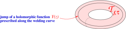
Figure 5: Inhomogeneous Riemann-Hilbert problem on $\,{\cal T}_{f,\tau}$

This may be viewed as an inhomogeneous Riemann-Hilbert problem RH on $\,{\cal T}_{f,\tau}\,$ searching for a holomorphic function with a prescribed jump along the $\,a$-curve of $\,{\cal T}_{f,\tau}\,$ which was obtained by welding the two edges of $\,{\cal A}_{f,\tau}$,  see Fig. 5.  As we shall see below, this problem has a solution $\,Y\,$ for a unique $\,\widehat{\tau}\in\mathbb{H}_{+}$,  assuming that $\,Y_{i}\in L^{2}(S^{1}_{L})$.  Besides such a solution is unique up to an additive constant, and $\,Y_{i}\,$ are automatically smooth. Given $\,Y$,  the function

$$W(z)=z\,{\rm e}^{\hskip 0.71114pt\frac{2\pi\mathrm{i}}{L}Y(z)}$$ (6.17)

on $\,{\cal A}_{f,\tau}\,$ has the boundary values $\,W_{i}=W\circ p_{i}\,$ that satisfy

$$W_{1}=\widehat{q}\,W_{2}$$ (6.18)

so that it defines a holomorphic map from $\,{\cal T}_{f,\tau}\,$ to $\,\mathbb{C}^{\times}\big{/}(w\sim\widehat{q}^{\pm 1}w)\cong{\cal T}_{f_{0},\widehat{\tau}}$. That map provides the isomorphism $\,{\cal T}_{f,\tau}\cong{\cal T}_{f_{0},\widehat{\tau}}$.

The solution of the inhomogeneous Riemann-Hilbert problem searching for the function $\,Y\,$ follows the standard strategy RH . In the interior of $\,{\cal A}_{f,\tau}$, $\,Y(z)\,$ is expressed in terms of its boundary values $\,Y_{i}\,$ via the Cauchy formula. Taking the limits $\,z\to p_{i}(x)\,$ in the latter and using (6.16),  one obtains a Fredholm equation for, say, $\,Y_{1}$.  Its solution, together with $\,Y_{2}\,$ obtained from (6.16),  and the Cauchy formula determine $\,Y$.

Here are some more details. Let us first assume that $\,Y_{i}\,$ are smooth. The Cauchy formula for $\,Y(z)\,$ with $\,z\,$ in the interior of $\,{\cal A}_{f,\tau}\,$ reads:

$$Y(z)\,=\,\frac{{}_{1}}{{}^{2\pi\mathrm{i}}}\int_{{\cal I}_{L}}\Big{(}\frac{Y_{1}(y)\,dp_{1}(y)}{p_{1}(y)-z}-\frac{Y_{2}(y)\,dp_{2}(y)}{p_{2}(y)-z}\Big{)}\,.$$ (6.19)

By sending $\,z\,$ to $\,p_{i}(x)$,  one obtains for the boundary values of $\,Y\,$ the relations

$$\frac{{}_{1}}{{}^{2}}Y_{1}(x)=\frac{{}_{1}}{{}^{2\pi\mathrm{i}}}\,PV\int_{{\cal I}_{L}}\frac{Y_{1}(y)\,dp_{1}(y)}{p_{1}(y)-p_{1}(x)}\,-\,\frac{{}_{1}}{{}^{2\pi\mathrm{i}}}\int_{{\cal I}_{L}}\frac{Y_{2}(y)\,dp_{2}(y)}{p_{2}(y)-p_{1}(x)}\,,$$ (6.20)

$$\frac{{}_{1}}{{}^{2}}Y_{2}(x)=\frac{{}_{1}}{{}^{2\pi\mathrm{i}}}\int_{{\cal I}_{L}}\frac{Y_{1}(y)\,dp_{1}(y)}{p_{1}(y)-p_{2}(x)}\,-\,\frac{{}_{1}}{{}^{2\pi\mathrm{i}}}\,PV\int_{{\cal I}_{L}}\frac{Y_{2}(y)\,dp_{2}(y)}{p_{2}(y)-p_{2}(x)}\,,$$ (6.21)

where $\,PV\,$ stands for “principal value”. We shall identify $L$-periodic functions on $\,\mathbb{R}\,$ with functions on the circle $\,{\mathbb{R}}/L{\mathbb{Z}}=S^{1}_{L}\,$ and shall denote by $\,E_{\pm}\,$ the orthogonal projections in $\,L^{2}(S^{1}_{L})\,$ on the subspace spanned by functions $\,e_{n}(x)=\frac{1}{\sqrt{L}}{\rm e}^{-\mathrm{i}p_{n}x}\,$ with $\,n>0\,$ and $\,n<0$,  respectively, for $\,p_{n}\equiv\frac{2\pi n}{L}$.  Similarly, we shall denote by $\,E_{0\pm}\,$ the orthogonal projections corresponding to $\,n\geq 0\,$ and $\,n\leq 0$.  For a smooth $\,L$-periodic function $\,X$, one has the relation

$$\frac{{}_{1}}{{}^{2}}\big{(}(E_{0+}-E_{-})X\big{)}(x)\,=\,-\frac{{}_{1}}{{}^{2\pi\mathrm{i}}}\,PV\int_{{\cal I}_{L}}\frac{X(y)\,dp_{2}(y)}{p_{2}(y)-p_{2}(x)}\,.$$ (6.22)

Adding (6.22) for $\,X=Y_{1}\,$ to (6.20) and subtracting it for $\,X=Y_{2}\,$ from (6.21),  we obtain the identities:

$$E_{0+}Y_{1}=K_{11}Y_{1}+K_{12}Y_{2}\,,\qquad E_{-}Y_{2}=K_{21}Y_{1}\,,$$ (6.23)

where

$$(K_{11}X)(x)\,=\,\frac{{}_{1}}{{}^{2\pi\mathrm{i}}}\int_{{\cal I}_{L}}X(y)\Big{(}\frac{dp_{1}(y)}{p_{1}(y)-p_{1}(x)}-\frac{dp_{2}(y)}{p_{2}(y)-p_{2}(x)}\Big{)},$$ (6.24)

$$(K_{12}X)(x)\,=\,-\frac{{}_{1}}{{}^{2\pi\mathrm{i}}}\int_{{\cal I}_{L}}X(y)\frac{dp_{2}(y)}{p_{2}(y)-p_{1}(x)}\,,$$ (6.25)

$$(K_{21}X)(x)\,=\,\frac{{}_{1}}{{}^{2\pi\mathrm{i}}}\int_{{\cal I}_{L}}X(y)\frac{dp_{1}(y)}{p_{1}(y)-p_{2}(x)}$$ (6.26)

are trace-class Simon operators on $\,L^{2}(S^{1}_{L})\,$ as they have smooth kernels and $\,S^{1}_{L}\,$ is a compact manifold Sugi ; Brisl .  We also have the representations:

$$K_{11}=E_{0+}-F^{-1}E_{0+}F=-E_{-}+F^{-1}E_{-}F\,,\qquad K_{12}=F^{-1}QE_{0+}\,,\qquad K_{21}=E_{-}Q^{-1}F\,,$$ (6.27)

where $\,(FX)(x)=X(f^{-1}(x))\,$ and $\,Qe_{n}=q^{n}e_{n}$.  By a limiting argument, the relations (6.23) also hold if $\,Y_{i}\in L^{2}(S^{1}_{L})$.  Summing the equations (6.23), substituting $\,Y_{2}=Y_{1}-Y_{12}\,$ and denoting

$$K=K_{11}+K_{12}+K_{21}\,,$$ (6.28)

we obtain the identity

$$(I-K)Y_{1}=(E_{-}-K_{12})Y_{12}$$ (6.29)

which is a Fredholm equation for $\,Y_{1}$,  given $\,Y_{12}$.  It appears that,  conversely,  if $\,Y_{1}\in L^{2}(S^{1}_{L})\,$ is a solution of (6.29) for some $\,Y_{12}\in L^{2}(S^{1}_{L})\,$ then there exists a holomorphic function $\,Y\,$ on $\,{\cal A}_{f,\tau}\,$ for which $\,Y_{1}\,$ and $\,Y_{2}=Y_{1}-Y_{12}\,$ are its boundary values. Besides, if $\,Y_{12}\,$ is smooth then so is $\,(E_{-}-K_{12})Y_{12}\,$ and $\,KY_{1}\,$ so that (6.29) implies that $\,Y_{1}\,$ is also smooth.

The Fredholm operator $\,I-K\,$ has only constants in its kernel. Indeed, if $\,(I-K)X_{1}=0\,$ for some $\,X_{1}\in L^{2}(S^{1}_{L})\,$ then there exists a function $\,X\,$ holomorphic on $\,{\cal A}_{f,\tau}\,$ with smooth boundary values $\,X_{1}\,$ and $\,X_{2}=X_{1}$.  Such $\,X\,$ defines a holomorphic function on the torus $\,{\cal T}_{f,\tau}\,$ and must be constant. Since the index of the Fredholm operator $\,I-K\,$ vanishes,  it follows that the image of $\,I-K\,$ is of codimension one. The solubility of (6.29) for $\,Y_{1}$,  given $\,Y_{12}$,  requires a fine tuning of the constant contribution to $\,Y_{12}$.  Let $\,\omega\,$ be a holomorphic $\,1$-form on $\,{\cal T}_{f,\tau}\,$ fixed by the normalization condition

$$\int_{a}\omega=1\,.$$ (6.30)

We shall identify $\,\omega\,$ with its pullback to $\,{\cal A}_{f,\tau}\,$ that satisfies the relation $\,p_{1}^{*}\omega=p_{2}^{*}\omega$.  If $\,Y_{12}\,$ is the difference of the boundary values of a function $\,Y\,$ holomorphic in the interior of $\,{\cal A}_{f,\tau}\,$ then, by the Stokes theorem,

$$\int_{{\cal I}_{L}}Y_{12}\hskip 0.71114pt\,p_{1}^{*}\omega=\int_{{\cal I}_{L}}Y_{1}\,p_{1}^{*}\omega-\int_{{\cal I}_{L}}Y_{2}\,p_{2}^{*}\omega=\int_{{\cal A}_{f,\tau}}d(Y\omega)\,=\,0\,.$$ (6.31)

One may show that this is also a sufficient condition for the solubility of (6.29) for $\,Y_{1}$,  given $\,Y_{12}\hskip 0.71114pt$.  For $\,Y_{12}\,$ of  (6.16),  it fixes uniquely $\,\widehat{\tau}$.  The form $\,\omega\,$ may be constructed as the pullback by $\,W\,$ given by (6.17) of the holomorphic form $\,-\frac{dw}{2\pi\mathrm{i}w}\,$ on $\,\mathbb{C}^{\times}\,$ (that descends to $\,\mathbb{C}^{\times}\big{/}(w\sim\widehat{q}^{\pm 1}w)$).  It follows that it is given by the formula

$$\omega=-\frac{dz}{2\pi\mathrm{i}z}-L^{-1}dY\,.$$ (6.32)

The integrability condition (6.31) takes then for $\,Y_{12}\,$ given by (6.16) the form of an implicit equation for $\,\widehat{\tau}\,$:

$$\widehat{\tau}=\tau-L^{-2}\int_{{\cal I}_{L}}(f-f_{0})(df-dY_{1})\,.$$ (6.33)

One also obtains from (6.13) and (6.32) the relation

$$\int_{b}\hskip 0.71114pt\omega=\tau-L^{-1}f(0)+L^{-1}Y_{12}(0)=\widehat{\tau}$$ (6.34)

which, together with (6.30), shows that $\,\widehat{\tau}\in\mathbb{H}_{+}\,$ and that the isomorphism $\,{\cal T}_{f,\tau}\cong{\cal T}_{f_{0},\widehat{\tau}}\,$ defined by $\,W\,$ of (6.17) intertwines the markings defined by (6.13).

It will be convenient to introduce the functions

$$X_{1}(x)=f(x)-Y_{1}(x)-L\tau\,,$$ (6.35)

(6.36)

$$X_{2}(x)=x-Y_{2}(x)=x-Y_{1}(x)+Y_{12}(x)=f(x)+L(\widehat{\tau}-\tau)-Y_{1}(x)=X_{1}(x)+L\widehat{\tau}$$ (6.37)

such that

$$W_{i}(x)={\rm e}^{-\frac{2\pi\mathrm{i}}{L}X_{i}(x)}\,.$$ (6.38)

for the boundary values $\,W_{i}\,$ of $\,W$. The functions $\,X_{i}\,$ and their derivatives satisfy the relations

$$X_{i}(x+L)=X_{i}(x)+L\,,\qquad X_{i}^{\prime}(x+L)=X_{i}^{\prime}(x)\,,\qquad X^{\prime}_{1}(x)=X^{\prime}_{2}(x)\,.$$ (6.39)

We shall need below the following identities.

Lemma 1.  One has:

$$\int_{{\cal I}_{L}}\big{(}X_{i}^{\prime}(x)\big{)}^{2}dx=\int_{{\cal I}_{L}}\frac{{}_{1}}{{}^{f^{\prime}(x)}}\,\big{(}X_{i}^{\prime}(x)\big{)}^{2}dx\,,$$ (6.40)

$$\int_{{\cal I}_{L}}(SX_{i})(x)\,dx=\int_{{\cal I}_{L}}\frac{{}_{1}}{{}^{f^{\prime}(x)}}\,\big{(}(SX_{i})(x)-(Sf)(x)\big{)}\,dx\,,$$ (6.41)

where $\,S\,$ denotes the Schwarzian derivative,  see (2.12).

Proof of Lemma 1.  Consider first the 1-form $\,\eta_{1}(z)=\big{(}\frac{W^{\prime}(z)}{W(z)}\big{)}^{2}z\hskip 0.71114ptdz\,$ on $\,{\cal A}_{f,\tau}$. One has

$$\int_{{\cal I}_{L}}p_{2}^{*}\eta_{1}=\big{(}-\frac{{}_{2\pi\mathrm{i}}}{{}^{L}}\big{)}\int_{{\cal I}_{L}}\big{(}X_{2}^{\prime}(x)\big{)}^{2}dx\,.$$ (6.42)

On the other hand,

$$\int_{{\cal I}_{L}}p_{1}^{*}\eta_{1}=\big{(}-\frac{{}_{2\pi\mathrm{i}}}{{}^{L}}\big{)}\int_{{\cal I}_{L}}\frac{{}_{1}}{{}^{f^{\prime}(x)}}\big{(}X_{1}^{\prime}(x)\big{)}^{2}dx$$ (6.43)

so that the identity (6.40) follows from the holomorphicity of the 1-form $\,\eta_{1}\,$ in the interior of $\,{\cal A}_{f,\tau}\hskip 0.71114pt$. Similarly,  consider the 1-form $\,\eta_{2}(z)=(SW)(z)\hskip 0.71114ptz\hskip 0.71114ptdz\,$ that is also holomorphic on the interior of $\,{\cal A}_{f,\tau}$.  Now one has:

$$\int_{{\cal I}_{L}}p_{2}^{*}\eta_{2}=\big{(}-\frac{{}_{2\pi\mathrm{i}}}{{}^{L}}\big{)}\int_{{\cal I}_{L}}\Big{(}-\frac{{}_{1}}{{}^{2}}\big{(}X^{\prime}_{2}(x)\big{)}^{2}-\frac{{}_{L^{2}}}{{}^{4\pi^{2}}}(SX_{2})(x)+\frac{{}_{1}}{{}^{2}}\Big{)}dx$$ (6.44)

and

$$\int_{{\cal I}_{L}}p_{1}^{*}\eta_{2}=\big{(}-\frac{{}_{2\pi\mathrm{i}}}{{}^{L}}\big{)}\int_{{\cal I}_{L}}\frac{{}_{1}}{{}^{f^{\prime}(x)}}\Big{(}-\frac{{}_{1}}{{}^{2}}\big{(}X^{\prime}_{1}(x)\big{)}^{2}-\frac{{}_{L^{2}}}{{}^{4\pi^{2}}}(SX_{1})(x)+\frac{{}_{L^{2}}}{{}^{4\pi^{2}}}(Sf)(x)+\frac{{}_{1}}{{}^{2}}f^{\prime}(x)^{2}\Big{)}\,dx$$ (6.45)

$$=\big{(}-\frac{{}_{2\pi\mathrm{i}}}{{}^{L}}\big{)}\int_{{\cal I}_{L}}\bigg{(}\frac{{}_{1}}{{}^{f^{\prime}(x)}}\Big{(}-\frac{{}_{1}}{{}^{2}}\big{(}X^{\prime}_{1}(x)\big{)}^{2}-\frac{{}_{L^{2}}}{{}^{4\pi^{2}}}(SX_{1})(x)+\frac{{}_{L^{2}}}{{}^{4\pi^{2}}}(Sf)(x)\Big{)}+\frac{{}_{1}}{{}^{2}}\bigg{)}\hskip 0.71114ptdx\,.$$ (6.46)

Comparing both integrals and using (6.40) and the equality $\,SX_{1}=SX_{2}$,  we obtain (6.41).

$\square$

D 1-point function of the Euclidian energy-momentum tensor

The holomorphic component of the Euclidian energy-momentum tensor is given by the formula

$$T^{E}(z)=\sum\limits_{n=-\infty}^{\infty}i^{n}L_{n}\hskip 0.71114ptz^{-n-2}\hskip 0.71114pt.$$ (6.47)

In view of (2.3), the Minkowskian energy-momentum tensor $\,T(x)\,$ is related to $\,T^{E}(z)\,$ for $\,|z|=1\,$ by the identity

$$T(x)=\frac{{}_{2\pi}}{{}^{L^{2}}}\Big{(}{\rm e}^{-\frac{4\pi\mathrm{i}}{L}x}\,T^{E}({\rm e}^{-\frac{2\pi\mathrm{i}}{L}x})-\frac{{}_{c}}{{}^{24}}\Big{)}$$ (6.48)

that we shall use below several times. We would like to find the 1-point function of $\,T^{E}(z)\,$ on the torus $\,{\cal T}_{f,\tau}\,$ defined as

$$\big{\langle}\,T^{E}(z)\hskip 0.71114pt\big{\rangle}_{{}_{{\cal T}_{f,\tau}}}\,=\,\frac{\hbox{Tr}\Big{(}U(f)\,T^{E}(z)\,\hskip 0.71114pt{\rm e}^{2\pi\mathrm{i}\tau(L_{0}-\frac{c}{24})}\Big{)}}{\hbox{Tr}\Big{(}U(f)\,\hskip 0.71114pt{\rm e}^{2\pi\mathrm{i}\tau(L_{0}-\frac{c}{24})}\Big{)}}\hskip 0.71114pt.$$ (6.49)

$\langle\,T^{E}(z)\hskip 0.71114pt\rangle_{{}_{{\cal T}_{f,\tau}}}$ is holomorphic in the interior of $\,{\cal A}_{f,\tau}\,$ and has boundary values,  at least in the distributional sense,  that we would like to relate. Since the commutator with $\,L_{0}-\frac{2}{24}\,$ generates the dilations of $\,T^{E}(z)\,$ so that.

$$q^{2}\hskip 0.71114ptT^{E}(qz)\,=\,{\rm e}^{2\pi\mathrm{i}\tau(L_{0}-\frac{c}{24})}\,T^{E}(z)\,{\rm e}^{-2\pi\mathrm{i}\tau(L_{0}-\frac{c}{24})}\hskip 0.71114pt,$$ (6.50)

we infer using (6.48) and the transformation rule (2.11) that

$$f^{\prime}(x)^{2}\,\Big{(}q^{2}\,{\rm e}^{-\frac{4\pi\mathrm{i}}{L}f(x)}\,\Big{\langle}\hskip 0.71114ptT^{E}(q\,{\rm e}^{-\frac{2\pi\mathrm{i}}{L}f(x)})\Big{\rangle}_{{}_{{\cal T}_{f,\tau}}}-\frac{{}_{c}}{{}^{24}}\Big{)}$$ (6.51)

(6.52)

(6.53)

$$=\frac{f^{\prime}(x)^{2}\,\hbox{Tr}\bigg{(}U(f)\,\Big{(}q^{2}\,{\rm e}^{-\frac{4\pi\mathrm{i}}{L}f(x)}\,T^{E}(q\,{\rm e}^{-\frac{2\pi\mathrm{i}}{L}f(x)})\,-\,\frac{c}{24}\Big{)}\,{\rm e}^{2\pi\mathrm{i}\tau(L_{0}-\frac{c}{24})}\bigg{)}}{\hbox{Tr}\Big{(}U(f)\,\hskip 0.71114pt{\rm e}^{2\pi\mathrm{i}\tau(L_{0}-\frac{c}{24})}\Big{)}}$$ (6.54)

$$=\,\frac{f^{\prime}(x)^{2}\,\hbox{Tr}\bigg{(}U(f)\,\hskip 0.71114pt{\rm e}^{2\pi\mathrm{i}\tau(L_{0}-\frac{c}{24})}\Big{(}{\rm e}^{-\frac{4\pi\mathrm{i}}{L}f(x)}\,T^{E}({\rm e}^{-\frac{2\pi\mathrm{i}}{L}f(x)})\,-\,\frac{c}{24}\Big{)}\bigg{)}}{\hbox{Tr}\Big{(}U(f)\,\hskip 0.71114pt{\rm e}^{2\pi\mathrm{i}\tau(L_{0}-\frac{c}{24})}\Big{)}}$$ (6.55)

$$=\,\frac{f^{\prime}(x)^{2}\,\hbox{Tr}\Big{(}U(f)\,\hskip 0.71114pt{\rm e}^{2\pi\mathrm{i}\tau(L_{0}-\frac{c}{24})}\,\frac{L^{2}}{2\pi}T(f(x))\Big{)}}{\hbox{Tr}\Big{(}U(f)\,\hskip 0.71114pt{\rm e}^{2\pi\mathrm{i}\tau(L_{0}-\frac{c}{24})}\Big{)}}\,=\,\frac{\frac{L^{2}}{2\pi}\,\hbox{Tr}\Big{(}f^{\prime}(x)^{2}\,T(f(x))\,U(f)\,\hskip 0.71114pt{\rm e}^{2\pi\mathrm{i}\tau(L_{0}-\frac{c}{24})}\Big{)}}{\hbox{Tr}\Big{(}U(f)\,\hskip 0.71114pt{\rm e}^{2\pi\mathrm{i}\tau(L_{0}-\frac{c}{24})}\Big{)}}$$ (6.56)

$$=\,\frac{\frac{L^{2}}{2\pi}\,\hbox{Tr}\bigg{(}\Big{(}f^{\prime}(x)^{2}T(f(x))-\frac{c}{24\pi}(Sf)(x)\Big{)}\,U(f)\,\hskip 0.71114pt{\rm e}^{2\pi\mathrm{i}\tau(L_{0}-\frac{c}{24})}\bigg{)}}{\hbox{Tr}\Big{(}U(f)\,\hskip 0.71114pt{\rm e}^{2\pi\mathrm{i}\tau(L_{0}-\frac{c}{24})}\Big{)}}\,+\,\frac{{}_{cL^{2}}}{{}^{48\pi^{2}}}(Sf)(x)$$ (6.57)

$$=\,\frac{\frac{L^{2}}{2\pi}\,\hbox{Tr}\Big{(}U(f)\,T(x)\,\hskip 0.71114pt{\rm e}^{2\pi\mathrm{i}\tau(L_{0}-\frac{c}{24})}\Big{)}}{\hbox{Tr}\Big{(}U(f)\,\hskip 0.71114pt{\rm e}^{2\pi\mathrm{i}\tau(L_{0}-\frac{c}{24})}\Big{)}}\,+\,\frac{{}_{cL^{2}}}{{}^{48\pi^{2}}}(Sf)(x)$$ (6.58)

$$=\,\frac{\hbox{Tr}\bigg{(}U(f)\,\Big{(}{\rm e}^{-\frac{4\pi\mathrm{i}}{L}x}T^{E}({\rm e}^{-\frac{2\pi\mathrm{i}}{L}x})-\frac{c}{24}\Big{)}\,{\rm e}^{2\pi\mathrm{i}\tau(L_{0}-\frac{c}{24})}\bigg{)}}{\hbox{Tr}\Big{(}U(f)\,\hskip 0.71114pt{\rm e}^{2\pi\mathrm{i}\tau(L_{0}-\frac{c}{24})}\Big{)}}\,+\,\frac{{}_{cL^{2}}}{{}^{48\pi^{2}}}(Sf)(x)$$ (6.59)

(6.60)

(6.61)

$$=\,{\rm e}^{-\frac{4\pi\mathrm{i}}{L}x}\,\Big{\langle}\hskip 0.71114ptT^{E}({\rm e}^{-\frac{2\pi\mathrm{i}}{L}x})\Big{\rangle}_{{}_{{\cal T}_{f,\tau}}}-\frac{{}_{c}}{{}^{24}}\,+\,\frac{{}_{cL^{2}}}{{}^{48\pi^{2}}}\,(Sf)(x)\,.$$ (6.62)

This is a linear inhomogeneous equation for the boundary values of the 1-point function $\,\langle\,T^{E}(z)\hskip 0.71114pt\rangle_{{}_{{\cal T}_{f,\tau}}}$.  Let us consider now the function

$$G(z)=\frac{{}_{c}}{{}^{12}}(SW)(z)\,,$$ (6.63)

where $\,W(z)\,$ is given by (6.17). By the chain rule for the Schwarzian derivative (2.13) and (6.18),

$$(SW_{1})(x)=\big{(}q(-\frac{{}_{2\pi\mathrm{i}}}{{}^{L}})f^{\prime}(x)\,{\rm e}^{-\frac{2\pi\mathrm{i}}{L}f(x)}\big{)}^{2}\,(SW)(q\,{\rm e}^{-\frac{2\pi\mathrm{i}}{L}f(x)})+\frac{{}_{2\pi^{2}}}{{}^{L^{2}}}\,f^{\prime}(x)^{2}+(Sf)(x)$$ (6.64)

$$=\,(SW_{2})(x)=\big{(}(-\frac{{}_{2\pi\mathrm{i}}}{{}^{L}})\,{\rm e}^{-\frac{2\pi\mathrm{i}}{L}x}\big{)}^{2}\,(SW)({\rm e}^{-\frac{2\pi\mathrm{i}}{L}x})+\frac{{}_{2\pi^{2}}}{{}^{L^{2}}}=-\frac{{}_{4\pi^{2}}}{{}^{L^{2}}}\big{(}{\rm e}^{-\frac{4\pi\mathrm{i}}{L}x}(SW)({\rm e}^{-\frac{2\pi\mathrm{i}}{L}x})-\frac{{}_{1}}{{}^{2}}\big{)}$$ (6.65)

from which we conclude that

$$f^{\prime}(x)^{2}\Big{(}q^{2}\,{\rm e}^{-\frac{4\pi\mathrm{i}}{L}f(x)}\,G(q\,{\rm e}^{-\frac{2\pi\mathrm{i}}{L}f(x)})-\frac{{}_{c}}{{}^{24}}\Big{)}\,=\,{\rm e}^{-\frac{4\pi\mathrm{i}}{L}x}\,G({\rm e}^{-\frac{2\pi\mathrm{i}}{L}x})-\frac{{}_{c}}{{}^{24}}+\frac{{}_{cL^{2}}}{{}^{48\pi^{2}}}\,(Sf)(x)\,,\qquad$$ (6.66)

which is the same linear inhomogeneous equation that for the boundary values of $\,\langle\,T^{E}(z)\hskip 0.71114pt\rangle_{{}_{{\cal T}_{f,\tau}}}$.  But the corresponding homogeneous equation for the boundary values of a holomorphic function $\,F(z)\,$ on the interior of $\,{\cal A}_{f,\tau}\hskip 0.71114pt$,

$$f^{\prime}(x)^{2}\,q^{2}\,{\rm e}^{-\frac{4\pi\mathrm{i}}{L}f(x)}\,F(q\,{\rm e}^{-\frac{2\pi\mathrm{i}}{L}f(x)})={\rm e}^{-\frac{4\pi\mathrm{i}}{L}x}\,F({\rm e}^{-\frac{2\pi\mathrm{i}}{L}x})\,,$$ (6.67)

has solutions that correspond to holomorphic quadratic differentials $\,F(z)(dz)^{2}\,$ pulled back from $\,{\cal T}_{f,\tau}\,$ that necessarily are of the form $\,A(d\ln{W(z)})^{2}$,  i.e.

$$F(z)=A\hskip 0.71114pt\Big{(}\frac{W^{\prime}(z)}{W(z)}\Big{)}^{2}$$ (6.68)

for some constant $\,A$.  This leads to the identity

$$\big{\langle}\,T^{E}(z)\hskip 0.71114pt\big{\rangle}_{{}_{{\cal T}_{f,\tau}}}=\,G(z)+F(z)\,=\,\frac{{}_{c}}{{}^{12}}\,(SW)(z)\,+\,F(z)\,.$$ (6.69)

The parameter $\,A\,$ in (6.68) may be fixed from the transformation rule of the Euclidian energy-momentum expectations between the isomorphic tori $\,{\cal T}_{f,\tau}\,$ and $\,{\cal T}_{f_{0},\widehat{\tau}}\,$ in Euclidian CFT which gives

$$F(z) = W^{\prime}(z)^{2}\,\big{\langle}\,T^{E}(W(z))\hskip 0.71114pt\big{\rangle}_{{}_{{\cal T}_{f_{0},\widehat{\tau}}}}\,,$$ (6.70)

see Eq. (5.124) in DFMS or (2.15) in KGPr .  Since

$$\big{\langle}\,T^{E}(w)\hskip 0.71114pt\big{\rangle}_{{}_{{\cal T}_{f_{0},\widehat{\tau}}}}\,=\,\frac{\hbox{Tr}\Big{(}T^{E}(w)\,\hskip 0.71114pt{\rm e}^{2\pi\mathrm{i}\widehat{\tau}(L_{0}-\frac{c}{24})}\Big{)}}{\hbox{Tr}\Big{(}{\rm e}^{2\pi\mathrm{i}\widehat{\tau}(L_{0}-\frac{c}{24})}\Big{)}}=\frac{\hbox{Tr}\Big{(}L_{0}\hskip 0.71114ptw^{-2}\,{\rm e}^{2\pi\mathrm{i}\widehat{\tau}(L_{0}-\frac{c}{24})}\Big{)}}{\hbox{Tr}\Big{(}{\rm e}^{2\pi\mathrm{i}\widehat{\tau}(L_{0}-\frac{c}{24})}\Big{)}}$$ (6.71)

$$=w^{-2}\bigg{(}\frac{\hbox{Tr}\Big{(}(L_{0}-\frac{c}{24})\,\hskip 0.71114pt{\rm e}^{2\pi\mathrm{i}\widehat{\tau}(L_{0}-\frac{c}{24})}\Big{)}}{\hbox{Tr}\Big{(}{\rm e}^{2\pi\mathrm{i}\widehat{\tau}(L_{0}-\frac{c}{24})}\Big{)}}+\frac{{}_{c}}{{}^{24}}\bigg{)}=w^{-2}\Big{(}\frac{{}_{1}}{{}^{2\pi\mathrm{i}}}\hskip 0.71114pt\partial_{\widehat{\tau}}\ln{\chi(\widehat{\tau})}+\frac{{}_{c}}{{}^{24}}\Big{)},\qquad$$ (6.72)

we obtain then the identity

$$\big{\langle}\,T^{E}(z)\hskip 0.71114pt\big{\rangle}_{{}_{{\cal T}_{f,\tau}}}\,=\,\frac{{}_{c}}{{}^{12}}\,(SW)(z)\,+\,\Big{(}\frac{W^{\prime}(z)}{W(z)}\Big{)}^{2}\Big{(}\frac{{}_{1}}{{}^{2\pi\mathrm{i}}}\,\partial_{\widehat{\tau}}\ln{\chi(\widehat{\tau})}+\frac{{}_{c}}{{}^{24}}\Big{)}$$ (6.73)

that is the main result of the present subsection.

E ${Diff_{+}{}^{{}^{\sim}}S^{1}}\,$ character on 1-parameter subgroups

We shall use the identity (6.73) to calculate the logarithmic $\hskip 0.71114pts$-derivative of

$$c_{s,\zeta}^{-1}\,\Upsilon(f_{s},\tau)=\hbox{Tr}\Big{(}{\rm e}^{\mathrm{i}s\int_{{\cal I}_{L}}\zeta(x)T(x)dx}\,\hskip 0.71114pt{\rm e}^{2\pi\mathrm{i}\tau(L_{0}-\frac{c}{24})}\Big{)}\,\equiv\,\widetilde{\Upsilon}(f_{s},\tau)$$ (6.74)

for the flow $\,f_{s}\,$ of the vector field $\,-\zeta(x)\partial_{x}$,  see (6.9) and (2.15). First note that

$$\partial_{s}\ln{\widetilde{\Upsilon}(f_{s},\tau)}\,=\,\frac{\mathrm{i}\int_{{\cal I}_{L}}\zeta(x)\,\hbox{Tr}\Big{(}U(f_{s})\,T(x)\,\hskip 0.71114pt{\rm e}^{2\pi\mathrm{i}\tau(L_{0}-\frac{c}{24})}\Big{)}\hskip 0.71114ptdx}{\hbox{Tr}\Big{(}U(f_{s})\,\hskip 0.71114pt{\rm e}^{2\pi\mathrm{i}\tau(L_{0}-\frac{c}{24})}\Big{)}}\,.$$ (6.75)

Denoting by $\,W_{s}\,$ the function defining the isomorphism $\,{\cal T}_{f_{s},\tau}\cong{\cal T}_{f_{0},\widehat{\tau}_{s}}\,$ constructed as in Sec. C and by $\,W_{s;i}={\rm e}^{-\frac{2\pi\mathrm{i}}{L}X_{s;i}}\,$ its boundary values such that $\,X_{s;1}=X_{s;2}-L\widehat{\tau}_{s}$,  we infer from (6.48), (6.73), (6.65) and (6.39) that

$$\frac{\frac{L^{2}}{2\pi}\,\hbox{Tr}\Big{(}U(f_{s})\,T(x)\,\hskip 0.71114pt{\rm e}^{2\pi\mathrm{i}(L_{0}-\frac{c}{24})}\Big{)}}{\hbox{Tr}\Big{(}U(f_{s})\,\hskip 0.71114pt{\rm e}^{2\pi\mathrm{i}(L_{0}-\frac{c}{24})}\Big{)}}\,=\,{\rm e}^{-\frac{4\pi\mathrm{i}}{L}x}\,\big{\langle}T^{E}({\rm e}^{-\frac{2\pi\mathrm{i}}{L}x})\big{\rangle}_{{}_{{\cal T}_{f,\tau}}}-\,\frac{{}_{c}}{{}^{24}}$$ (6.76)

$$=\,\frac{{}_{c}}{{}^{12}}\,{\rm e}^{-\frac{4\pi\mathrm{i}}{L}x}\,(SW_{s})({\rm e}^{-\frac{2\pi\mathrm{i}}{L}x})\,+\,{\rm e}^{-\frac{4\pi\mathrm{i}}{L}x}\,\Big{(}\frac{W^{\prime}_{s}({\rm e}^{-\frac{2\pi\mathrm{i}}{L}x})}{W_{s}({\rm e}^{-\frac{2\pi\mathrm{i}}{L}x})}\Big{)}^{2}\Big{(}\frac{{}_{1}}{{}^{2\pi\mathrm{i}}}\,\partial_{\widehat{\tau}_{s}}\ln{\chi(\widehat{\tau}_{s})}+\frac{{}_{c}}{{}^{24}}\Big{)}\,-\,\frac{{}_{c}}{{}^{24}}$$ (6.77)

$$=\,-\frac{{}_{cL^{2}}}{{}^{48\pi^{2}}}\,(SW_{s;2})(x)\,-\,\frac{{}_{L^{2}}}{{}^{4\pi^{2}}}\,\big{(}\partial_{x}\ln{W_{s;2}(x)}\big{)}^{2}\,\Big{(}\frac{{}_{1}}{{}^{2\pi\mathrm{i}}}\,\partial_{\widehat{\tau}_{s}}\ln{\chi(\widehat{\tau}_{s})}+\frac{{}_{c}}{{}^{24}}\Big{)}$$ (6.78)

(6.79)

$$=\,-\frac{{}_{cL^{2}}}{{}^{48\pi^{2}}}\,(SX_{s;i})(x)+\frac{{}_{1}}{{}^{2\pi\mathrm{i}}}\,(X^{\prime}_{s;i}(x))^{2}\,\partial_{\widehat{\tau}_{s}}\ln{\chi(\widehat{\tau}_{s})}\,.$$ (6.80)

The substitution of (6.80) to (6.75) gives then the relation

$$\partial_{s}\ln{\widetilde{\Upsilon}(f_{s},\tau)}\,=\,-\mathrm{i}\,\frac{{}_{c}}{{}^{24\pi}}\int_{{\cal I}_{L}}\zeta(x)\,(SX_{s;i})(x)\,dx\,+\,L^{-2}\int_{{\cal I}_{L}}\zeta(x)\,(X^{\prime}_{s;i}(x))^{2}\hskip 0.71114ptdx\ \,\partial_{\widehat{\tau}_{s}}\ln{\chi(\widehat{\tau}_{s})}\,.$$ (6.81)

In the next subsection, we shall show that

$$\partial_{s}\widehat{\tau}_{s}=\,L^{-2}\int_{{\cal I}_{L}}\zeta(x)\,(X^{\prime}_{s;i}(x))^{2}\hskip 0.71114ptdx\,.$$ (6.82)

Using this identity, we infer from (6.81) that

$$\Upsilon(f_{s},\tau)\,=\,C_{f_{s},\tau}\,\chi(\widehat{\tau}_{s})$$ (6.83)

with

$$C_{f_{s},\tau}\,=\,c_{s,\zeta}\,\hskip 0.71114pt\exp\bigg{[}-\mathrm{i}\frac{{}_{c}}{{}^{24\pi}}\int_{0}^{s}ds^{\prime}\int_{{\cal I}_{L}}\zeta(x)\hskip 0.71114pt(SX_{s^{\prime},i})(x)\,dx\hskip 0.71114pt\bigg{]}.$$ (6.84)

This establishes the relation between the characters of $\,{Diff_{+}{}^{{}^{\sim}}S^{1}}\,$ on 1-parameter subgroups and the Virasoro characters.

Remark.  We could obtain formulae similar to (6.81) and (6.82) if we replaced $\,f_{s}\,$ by $\,f\circ f_{s}\,$ for any $\,f\in{Diff_{+}{}^{{}^{\sim}}S^{1}}$.  This would lead to an expression for $\,\Upsilon(f,\tau)\,$ involving the integration along any smooth curve joining $\,f\,$ to $\,f_{0}$,  but we shall not need such a generalization here.

F The effective modular parameter

In this subsection, we shall obtain an integral expression for the effective modular parameter $\,\widehat{\tau}_{s}\,$ such that $\,{\cal T}_{f_{s},\tau}\cong{\cal T}_{f_{0},\widehat{\tau}_{s}}$.  With the applications to FCS in sight,  we shall consider a slightly more general situation with the initial modular parameter $\,\tau\,$ replaced by $\,\tau_{s}=\tau-L^{-1}as\,$ for some real constant $\,a$.  Let $\,W_{s}:{\cal A}_{f_{s},\tau_{s}}\rightarrow\mathbb{C}^{\times}\,$ be the map constructed as in Sec. C defining the isomorphism $\,{\cal T}_{f_{s},\tau_{s}}\cong{\cal T}_{f_{0},\widehat{\tau}_{s}}\,$ with the boundary values $\,W_{s;i}={\rm e}^{-\frac{2\pi\mathrm{i}}{L}X_{s;i}}\,$ such that $\,X_{s;1}(x)=X_{s;2}(x)-L\widehat{\tau}_{s}$. Clearly, $\,X_{s;i}\,$ and $\,\widehat{\tau}_{s}\,$ depend now also on $\,a$.

Proposition.  The effective modular parameter $\,\widehat{\tau}_{s}\,$ satisfies the relation

$$\partial_{s}\widehat{\tau}_{s}=\hskip 0.71114ptL^{-2}\int_{{\cal I}_{L}}\big{(}\zeta(x)-a\big{)}\hskip 0.71114pt(X^{\prime}_{s;i}(x))^{2}\hskip 0.71114ptdx$$ (6.85)

Proof of Proposition.  Eq. (6.85) will be established by calculating the infinitesimal change in $\,\widehat{\tau}_{s}$.  Denote by $\,{\cal A}_{s}\,$ the annular region in $\,\mathbb{C}^{\times}\,$ that is the image of $\,{\cal A}_{f_{s},\tau_{s}}\,$ by $\,W_{s}\,$ and has the boundary components parameterized by

$$x\ \longmapsto\ W_{s}(q_{s}\hskip 0.85355pt{\rm e}^{-\frac{2\pi\mathrm{i}}{L}f_{s}(x)})={\rm e}^{-\frac{2\pi\mathrm{i}}{L}X_{s;1}(x)}\,,\qquad x\ \longmapsto\ W_{s}({\rm e}^{-\frac{2\pi\mathrm{i}}{L}x})={\rm e}^{-\frac{2\pi\mathrm{i}}{L}X_{s;2}(x)}$$ (6.86)

for $\,q_{s}={\rm e}^{2\pi\mathrm{i}\tau_{s}}$.  Consider the map $\,U_{s,\sigma}=W_{s+\sigma}\circ W_{s}^{-1}:{\cal A}_{s}\rightarrow\mathbb{C}^{\times}\,$ that is holomorphic on the interior of $\,{\cal A}_{s}\,$ and that satisfies the relations

$$U_{s,\sigma}({\rm e}^{-\frac{2\pi\mathrm{i}}{L}X_{s;1}(f_{s}^{-1}(f_{s+\sigma}(x)+a\sigma))})=W_{s+\sigma}(q_{s+\sigma}\,{\rm e}^{-\frac{2\pi\mathrm{i}}{L}f_{s+\sigma}(x)})={\rm e}^{-\frac{2\pi\mathrm{i}}{L}X_{s+\sigma;1}(x)}$$ (6.87)

$$=\widehat{q}_{s+\sigma}\,{\rm e}^{-\frac{2\pi\mathrm{i}}{L}X_{s+\sigma;2}(x)}=\widehat{q}_{s+\sigma}\,W_{s+\sigma}({\rm e}^{-\frac{2\pi\mathrm{i}}{L}x})=\widehat{q}_{s+\sigma}\,U_{s,\sigma}({\rm e}^{-\frac{2\pi\mathrm{i}}{L}X_{s;2}(x)})$$ (6.88)

for $\,\widehat{q}_{s}={\rm e}^{2\pi\mathrm{i}\widehat{\tau}_{s}}$.  One may write

$$U_{s,\sigma}(w)=w\,{\rm e}^{\frac{2\pi\mathrm{i}}{L}V_{s,\sigma}(w)}\,,$$ (6.89)

where $\,V\,$ is a function on $\,{\cal A}_{s}\,$ with the boundary values

$$V_{s,\sigma;1}(x)\equiv V_{s,\sigma}({\rm e}^{-\frac{2\pi\mathrm{i}}{L}X_{s;1}(f_{s}^{-1}(f_{s+\sigma}(x)+a\sigma))})=X_{s;1}(f_{s}^{-1}(f_{s+\sigma}(x)+a\sigma))-X_{s+\sigma;1}(x)\,,$$ (6.90)

$$V_{s,\sigma;2}(x)\equiv V_{s,\sigma}({\rm e}^{-\frac{2\pi\mathrm{i}}{L}X_{s;2}(x)})=X_{s;2}(x)-X_{s+\sigma;2}(x)$$ (6.91)

so that

$$V_{s,\sigma;12}(x)\equiv V_{s,\sigma;1}(x)-V_{s,\sigma;2}(x) = X_{s;1}(f_{s}^{-1}(f_{s+\sigma}(x)+a\sigma))-X_{s;2}(x)+L\widehat{\tau}_{s+\sigma}$$ (6.92)

$$= X_{s;2}(f_{s}^{-1}(f_{s+\sigma}(x)+a\sigma))-X_{s;2}(x)+L(\widehat{\tau}_{s+\sigma}-\widehat{\tau}_{s})\,.$$ (6.93)

Consider on $\,{\cal A}_{s}\,$ the holomorphic form

$$\omega_{s,\sigma}=U_{s,\sigma}^{\hskip 0.71114pt*}\big{(}-\frac{{}_{du}}{{}^{2\pi\mathrm{i}u}}\big{)}=-\frac{{}_{dw}}{{}^{2\pi\mathrm{i}w}}-L^{-1}dV_{s,\sigma}\,.$$ (6.94)

Then

$$\omega_{s,\sigma}\big{(}{\rm e}^{-\frac{2\pi\mathrm{i}}{L}X_{s;1}(f_{s}^{-1}(f_{s+\sigma}(x)+a\sigma))}\big{)}\hskip 0.71114pt=\,\omega_{s,\sigma}\big{(}{\rm e}^{-\frac{2\pi\mathrm{i}}{L}X_{s;2}(x)}\big{)}=L^{-1}\hskip 0.71114pt\big{(}X^{\prime}_{s;2}(x)\,dx\,-\,V^{\prime}_{s,\sigma;2}(x)\big{)}\,dx\,,$$ (6.95)

where the first equality follows from (6.88).  Besides, $\,\omega_{s,\sigma}\,$ satisfies the normalization condition

$$\int_{{\cal I}_{L}}\omega_{s,\sigma}\big{(}{\rm e}^{-\frac{2\pi\mathrm{i}}{L}X_{s;2}(x)}\big{)}\,=\,1\,.$$ (6.96)

As $\,V_{s,\sigma}\,$ is a holomorphic on the interior of $\,{\cal A}_{s}$,  we have the relation

$$0 = \int_{{\cal A}_{s}}d\hskip 0.71114pt(V_{s,\sigma}\hskip 0.71114pt\omega_{s,\sigma})\,=\,\int_{{\cal I}_{L}}V_{s,\sigma;1}(x)\,\omega_{s,\sigma}\big{(}{\rm e}^{-\frac{2\pi\mathrm{i}}{L}X_{s;1}(f_{s}^{-1}(f_{s+\sigma}(x)+a\sigma))}\big{)}-\int_{{\cal I}_{L}}V_{s,\sigma;2}(x)\,\omega_{s,\sigma}\big{(}{\rm e}^{-\frac{2\pi\mathrm{i}}{L}X_{s;2}(x)}\big{)}$$ (6.97)

$$= \int_{{\cal I}_{L}}V_{s,\sigma;12}(x)\,\omega_{s,\sigma}\big{(}{\rm e}^{-\frac{2\pi\mathrm{i}}{L}X_{s;2}(x)}\big{)}$$ (6.98)

$$= \int_{{\cal I}_{L}}\Big{(}X_{s;2}(f_{s}^{-1}(f_{s+\sigma}(x)+a\sigma))-X_{s;2}(x)\Big{)}\,\omega_{s,\sigma}\big{(}{\rm e}^{-\frac{2\pi\mathrm{i}}{L}X_{s;2}(x)}\big{)}\,+\,L(\widehat{\tau}_{s+\sigma}-\widehat{\tau}_{s})$$ (6.99)

$$= L^{-1}\int_{{\cal I}_{L}}\Big{(}X_{s;2}(f_{s}^{-1}(f_{s+\sigma}(x)+a\sigma))-X_{s;2}(x)\Big{)}\Big{(}X^{\prime}_{s;2}(x)-V_{s,\sigma;2}^{\prime}(x)\Big{)}\hskip 0.71114ptdx\,+\,L(\widehat{\tau}_{s+\sigma}-\widehat{\tau}_{s})\hskip 0.71114pt.$$ (6.100)

Differentiating the last line over $\,\sigma\,$ at $\,\sigma=0\,$ and using the fact that $\,V_{s,0}=0$,  as well as the relation

$$(f_{s}^{-1})^{\prime}(f_{s}(x))\,\zeta(f_{s}(x))=\zeta(x)$$ (6.101)

that follows from the differentiation over $\,s\,$ of the identity $\,f_{s}^{-1}(f_{s}(x))=x$,  we infer from (6.100) that

$$0 = L^{-1}\int_{{\cal I}_{L}}X^{\prime}_{s;2}(x)\,(f_{s}^{-1})^{\prime}(f_{s}(x))\big{(}-\zeta(f_{s}(x))+a\big{)}\,X^{\prime}_{s;2}(x)\,dx\,+\,L\,\partial_{s}\widehat{\tau}_{s}$$ (6.102)

$$= -\,L^{-1}\int_{{\cal I}_{L}}(\zeta(x)-\frac{{}_{a}}{f^{\prime}_{s}(x)})\,(X^{\prime}_{s;2}(x))^{2}\,+\,L\,\partial_{s}\widehat{\tau}_{s}\,.$$ (6.103)

Together with (6.40),  this implies (6.85).

$\square$

Corollary.  Taking $\,a=0$,  we obtain (6.82).

G Generating function of FCS in finite volume

We are now ready to eliminate the $\,{Diff_{+}{}^{{}^{\sim}}S^{1}}$-character $\,\Upsilon(f_{s,t,L},\tau_{s,L})\,$ from the expression (6.10) for the finite-volume generating function $\,\Psi_{t,L}(\lambda)\,$ of  FCS for energy transfers.  To this end, we first rewrite the formula (6.10) in the form

$$\Psi_{t,L}(\lambda)\,=\,\frac{\widetilde{\Upsilon}(f_{s,t,L}\hskip 0.71114pt,\tau_{s,L})}{\chi(\tau_{0,L})}\,\,{\rm e}^{-\mathrm{i}s\hskip 0.71114pt(C_{t,L}-C_{0,L})}$$ (6.104)

recalling that

$$s=\frac{{}_{\lambda}}{{}^{\Delta\beta}}\,,\qquad\tau_{s,L}=L^{-1}(\mathrm{i}-s)\gamma_{L}\,,\qquad\zeta_{t,L}(x)=\gamma_{L}\frac{\beta_{L}(h_{L}^{-1}(x)+vt)}{\beta_{L}(h_{L}^{-1}(x))}$$ (6.105)

and $\,f_{s,t,L}\,$ is the flow of the vector field $\,-\zeta_{t,L}(x)\partial_{x}$. The only difference with respect to the setting of Sec. E is that $\,\tau\,$ is now replaced by $\,\tau_{s,L}\,$ which corresponds to the situation considered in Sec. F if we set $\,a=\gamma_{L}\,$ there.  Differentiating $\,\ln{\Psi_{t,L}}\,$ over $\,\lambda$,  we obtain the relation

$$\partial_{\lambda}\ln{\Psi_{t,L}(\lambda)}$$ (6.106)

$$=\,\frac{{}_{1}}{{}^{\Delta\beta}}\bigg{(}-\mathrm{i}\,\frac{{}_{c}}{{}^{24\pi}}\int_{{\cal I}_{L}}\zeta_{t,L}(x)\,(SX_{s,t,L;i})(x)\,dx\,+\,L^{-2}\int_{{\cal I}_{L}}\zeta_{t,L}(x)\,(X^{\prime}_{s,t,L;i}(x))^{2}\hskip 0.71114ptdx\ \,\partial_{\widehat{\tau}_{s,L,t}}\ln{\chi(\widehat{\tau}_{s,L,t})}$$ (6.107)

$$\hskip 36.98866pt-\,2\pi\mathrm{i}L^{-1}\gamma_{L}\frac{\hbox{Tr}\Big{(}U(f_{s,L,t})\,(L_{0}-\frac{c}{24})\,\hskip 0.71114pt{\rm e}^{2\pi\mathrm{i}\tau_{s,L}(L_{0}-\frac{c}{24})}\Big{)}}{\hbox{Tr}\Big{(}U(f_{s,L,t})\,\hskip 0.71114pt{\rm e}^{2\pi\mathrm{i}\tau_{s,L}(L_{0}-\frac{c}{24})}\Big{)}}\,-\,\mathrm{i}\,\big{(}C_{t,L}-C_{0,L}\big{)}\bigg{)},$$ (6.108)

where the $\,1^{\rm st}$-line on the right-hand side came from the $\,s$-dependence of $\,f_{s,t,L}\,$ in $\,\ln{\widetilde{\Upsilon}(f_{s,t,L},\tau_{s,L})}\,$ given by (6.81)  and the $\,1^{\rm st}\,$ term of the $\hskip 0.71114pt2^{\rm nd}$-line from the $\hskip 0.71114pts$-dependence of $\,\tau_{s,L}$.  Functions $\,X_{s,t,L;i}\,$ pertain to the boundary values of the maps $\,W_{s,t,L}\,$ defining the isomorphisms $\,{\cal T}_{f_{s,t,L},\tau_{s,L}}\cong{\cal T}_{f_{0},\widehat{\tau}_{s,t,L}}$,  see Sec. E.  Now,  from  (6.80),

$$\frac{2\pi\mathrm{i}L^{-1}\,\hbox{Tr}\Big{(}U(f_{s,L,t})\,(L_{0}-\frac{c}{24})\,\hskip 0.71114pt{\rm e}^{2\pi\mathrm{i}\tau_{s}(L_{0}-\frac{c}{24})}\Big{)}}{\hbox{Tr}\Big{(}{\rm e}^{2\pi\mathrm{i}\tau_{s}(L_{0}-\frac{c}{24})}\,U(f_{s,L,t})\Big{)}}=\frac{\mathrm{i}\,\hbox{Tr}\Big{(}U(f_{s,L,t})\int_{{\cal I}_{L}}T(x)\hskip 0.71114ptdx\,\,{\rm e}^{2\pi\mathrm{i}\tau_{s}(L_{0}-\frac{c}{24})}\Big{)}}{\hbox{Tr}\Big{(}{\rm e}^{2\pi\mathrm{i}\tau_{s}(L_{0}-\frac{c}{24})}\,U(f_{s,L,t})\Big{)}}$$ (6.109)

$$=\,-\mathrm{i}\,\frac{{}_{c}}{{}^{24\pi}}\int_{{\cal I}_{L}}(SX_{s,t,L;i})(x)dx\,+\,L^{-2}\int_{{\cal I}_{L}}(X^{\prime}_{s,t,L;i}(x))^{2}\hskip 0.71114ptdx\ \,\partial_{\widehat{\tau}_{s,L,t}}\ln{\chi(\widehat{\tau}_{s,L,t})}\,.$$ (6.110)

Thus the net effect of the $1^{\rm st}$ term on the $2^{\rm nd}$ line on the right-hand side of (6.108) is to replace $\,\zeta_{t,L}\,$ in the $1^{\rm nd}$ line by

$$\xi_{t,L}=\zeta_{t,L}-\gamma_{L}\,.$$ (6.111)

Altogether, we obtain the identity

$$\partial_{\lambda}\ln{\Psi_{t,L}(\lambda)} = \frac{{}_{1}}{{}^{\Delta\beta}}\bigg{(}-\mathrm{i}\,\frac{{}_{c}}{{}^{24\pi}}\int_{{\cal I}_{L}}\xi_{t,L}(x)\,(SX_{s,t,L;i})(x)\,dx$$ (6.113)

$$\hskip 25.6073pt+\,L^{-2}\int_{{\cal I}_{L}}\xi_{t,L}(x)\,(X^{\prime}_{s,t,L;i}(x))^{2}\hskip 0.71114ptdx\ \,\partial_{\widehat{\tau}_{s,t,L}}\ln{\chi(\widehat{\tau}_{s,t,L})}\,-\,\mathrm{i}\hskip 0.71114pt\big{(}C_{t,L}-C_{0,L}\big{)}\bigg{)}.$$

Moreover,  taking $\,\zeta=\zeta_{t,L}\,$ and $\,a=\gamma_{L}\,$ in Proposition of Sec. F,  we infer from (6.85) that

$$\partial_{s}\widehat{\tau}_{s,t,L}=L^{-2}\int_{{\cal I}_{L}}\xi_{t,L}(x)\,(X_{s,t,L;i}^{\prime}(x))^{2}\hskip 0.71114ptdx$$ (6.114)

so that (6.113) implies that

$$\Psi_{t,L}(\lambda)\,=\,\exp\bigg{[}-\mathrm{i}\,\frac{{}_{c}}{{}^{24\pi}}\int_{0}^{\frac{\lambda}{\Delta\beta}}ds\int_{{\cal I}_{L}}\xi_{t,L}(x)(SX_{s,t,L;i})(x)\,dx\bigg{]}\,\,\frac{\chi(\widehat{\tau}_{\frac{\lambda}{\Delta\beta},t,L})}{\chi(\tau_{0,L})}\,\,\hskip 0.71114pt{\rm e}^{-\hskip 0.71114pt\frac{\mathrm{i}\lambda}{\Delta\beta}\big{(}C_{t,L}-C_{0,L}\big{)}}\,,\qquad$$ (6.115)

where

$$\widehat{\tau}_{\frac{\lambda}{\Delta\beta},t,L}\,=\,\tau_{0,L}\,+\,L^{-2}\int_{0}^{\frac{\lambda}{\Delta\beta}}ds\int_{{\cal I}_{L}}\xi_{t,L}(x)\,(X_{s,t,L;i}^{\prime}(x))^{2}\hskip 0.71114ptdx$$ (6.116)

and $\,C_{t,L}\,$ is given by (4.14).  This is our final formula based on conformal welding for the finite-volume generating function for FCS of energy transfers. Note that the right-hand side of (6.115) depends on the spectrum of the CFT via the Virasoro character $\,\chi$.

7 Thermodynamic limit formula for FCS

We would like to compute the limit $\,L\to\infty\,$ of the generating function $\,\Psi_{t,L}(\lambda)\,$ for FCS. Let us first consider the last factor on the right hand side of (6.115). Using the symmetries (4.3) and (4.11) of $\,\beta_{L}\,$ and $\,h_{L}\,$ and the behavior of the latter when $\,L\to\infty$,  see (4.29),  we infer that

$$\lim\limits_{L\to\infty}\,{\rm e}^{-\frac{\mathrm{i}\lambda}{\Delta\beta}\big{(}C_{t,L}-C_{0,L}\big{)}} = \lim\limits_{L\to\infty}\,\exp\Big{[}{-\frac{{}_{\mathrm{i}\lambda}}{{}^{\Delta\beta}}\frac{{}_{cv}}{{}^{24\pi}}\int_{-{\frac{{}_{3}}{{}^{4}}L}}^{{\frac{{}_{1}}{{}^{4}}L}}(\beta_{L}(x^{+})-\beta_{L}(x))\,(Sh_{L})(x)\,dx}\Big{]}$$ (7.1)

$$= \exp\Big{[}{-\frac{{}_{\mathrm{i}\lambda}}{{}^{\Delta\beta}}\hskip 0.71114pt\frac{{}_{cv}}{{}^{24\pi}}\int(\beta(x^{+})+\beta(x^{-})-2\beta(x))\,(Sh)(x)\,dx}\Big{]},$$ (7.3)

where $\,h\,$ is given by (4.38) and (4.27). Note that the integral on the right hand side is concentrated on the support of the kink in the profile $\,\beta(x)$.

A Large $\,L\,$ behavior of the vector field $\,\zeta_{t,L}(y)\partial_{y}\,$ and of its flow

In order to study the limiting behavior of the other terms in the formula (6.115) for $\,\Psi_{t,L}(\lambda)$,  we shall need more detailed information about the forms of the inverse function $\,h_{L}^{-1}\,$ and of $\,\zeta_{t,L}\,$ given by (4.15).  Let us assume that $\,\beta(x)\,$ takes its asymptotic values outside the interval $\,[a-\delta,a+\delta]\,$ containing the kink. Then on the interval $\,[-\frac{1}{4}L,\frac{1}{4}L]$,  the function $\,h_{L}^{-1}\,$ is linear to the left and to the right of the interval $\,[A_{L},B_{L}]\,$

$$h_{L}^{-1}(y)\,=\,\begin{cases}\,\frac{\beta_{\cal L}}{\beta_{0,L}}(y+\frac{1}{4}L)-\frac{1}{4}L\qquad\text{for}\quad-\frac{1}{4}L\leq y\leq A_{L}\hskip 0.71114pt,\cr\,\frac{\beta_{\cal R}}{\beta_{0,L}}(y-\frac{1}{4}L)+\frac{1}{4}L\qquad\text{for}\hskip 22.1931ptB_{L}\leq y\leq\frac{1}{4}L\end{cases}$$ (7.4)

for

$$A_{L}=h_{L}(a-\delta)=\frac{{}_{\beta_{0,L}}}{{}^{\beta_{\cal L}}}(a-\delta)-\big{(}1-\frac{{}_{\beta_{0.L}}}{{}^{\beta_{\cal L}}})\frac{{}_{L}}{{}^{4}}\hskip 0.71114pt,\quad\ B_{L}=h_{L}(a+\delta)=\frac{{}_{\beta_{0,L}}}{{}^{\beta_{\cal R}}}(a+\delta)+\big{(}1-\frac{{}_{\beta_{0.L}}}{{}^{\beta_{\cal R}}})\frac{{}_{L}}{{}^{4}}\hskip 0.71114pt,$$ (7.5)

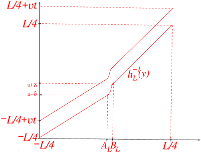
Figure 6: $\,h_{L}^{-1}\,$ and $\,h_{L}^{-1}+vt$

see Fig. 6,  and its form stabilizes inside that interval. More exactly, with the function $\,h(x)\,$ given by (4.38) and (4.27) and

$$A=h(a-\delta)\hskip 0.71114pt,\qquad B=h(a+\delta)\hskip 0.71114pt,$$ (7.6)

and for

$$O_{L}^{+}=-A+A_{L}\hskip 0.71114pt,$$ (7.7)

we have the identity

$$h_{L}^{-1}\big{(}y+O_{L}^{+}\big{)}=h^{-1}\big{(}\frac{{}_{\beta_{0}}}{{}^{\beta_{0,L}}}y+(1-\frac{{}_{\beta_{0}}}{{}^{\beta_{0,L}}})A\big{)}$$ (7.8)

so that by (4.26)

$$\lim\limits_{L\to\infty}\,h_{L}^{-1}(y+O_{L}^{+})=h^{-1}(y)\hskip 0.71114pt,$$ (7.9)

and the difference between $\,h_{L}^{-1}(y+O_{L}^{+})\,$ and $\,h^{-1}(y)\,$ is $\,O(L^{-1})\,$ uniformly for $\,y\,$ in bounded sets and the same is true for all the $\,y$-derivatives of that difference. The inverse function $\,h^{-1}\,$ is linear on the left and on the right of the interval $\,[A,B]\,$ and it maps this interval into $\,[a-\delta,a+\delta]$.  More precisely,

$$h^{-1}(y)\,=\,\begin{cases}\,\frac{\beta_{\cal L}}{\beta_{0}}(y-A)+a-\delta\qquad\,\text{for}\qquad y\leq A\,,\cr\,\frac{\beta_{\cal R}}{\beta_{0}}(y-B)+a+\delta\qquad\text{for}\qquad y\geq B\,,\end{cases}$$ (7.10)

An examination of the function $\,\zeta_{t,L}\,$ of (4.15) shows now that if $\,|x|\leq\frac{1}{4}L\,$ then $\,\zeta_{t,L}(x)=v\beta_{0,L}=\gamma_{L}\,$ outside an interval $\,[A_{L}-O(|t|),B_{L}+O(|t|)]\,$ and that the form of $\,\zeta_{t,L}\,$ stabilizes inside this interval. More precisely,

$$\zeta_{t,L}(y+O_{L}^{+})=\gamma_{L}\frac{\beta(h_{L}^{-1}(y+O_{L}^{+})+vt)}{\beta(h_{L}^{-1}(y+O_{L}^{+}))}$$ (7.11)

for large $\,L\,$ so that

$$\lim\limits_{L\to\infty}\,\zeta_{t,L}(y+O_{L}^{+})=\gamma\hskip 0.71114pt\frac{\beta\big{(}h^{-1}(y)+vt\big{)}}{\beta\big{(}h^{-1}(y)\big{)}}\equiv\zeta^{+}_{t}(y)$$ (7.12)

for $\,\gamma=v\beta_{0}\,$ with $\,\zeta^{+}_{t}(y)=\gamma\,$ outside an interval $\,[A-O(|t|),B+O(|t|)]$.  Similarly, for $\,\xi_{t,L}\,$ given by (6.111),

$$\lim\limits_{L\to\infty}\,\xi_{t,L}(y+O_{L}^{+})=\zeta^{+}_{t}(y)-\gamma\equiv\xi^{+}_{t}(y)$$ (7.13)

with $\,\xi^{+}_{t}(y)\,$ vanishing outside $\,[A-O(|t|),B+O(|t|)]$.  In particular, if $\,vt\geq 2\delta\,$ then

$$\xi^{+}_{t}(y)\,=\,\begin{cases}\,0\hskip 45.52458pt\text{for}\hskip 93.325pty\leq A-\frac{\beta_{0}}{\beta{\cal L}}vt\hskip 0.71114pt,\cr\,\gamma\frac{\Delta\beta}{\beta_{\cal L}}\hskip 29.87547pt\text{for}\quad A-\frac{\beta_{0}}{\beta_{\cal L}}(vt-2\delta)\leq y\leq A\hskip 0.71114pt,\cr\,0\hskip 44.9554pt\text{for}\hskip 73.12378ptB\leq y\hskip 0.71114pt.\end{cases}$$ (7.14)

The functions $\,f_{s,t,L}\,$ forming the flow of the vector field $\,-\zeta_{t,L}(y)\partial_{y}\,$ are equal to $\,f_{0}-\gamma_{L}s\,$ outside an interval $\,[A_{L}-O(|t|+|s|),B_{L}+O(|t|+|s|)]\,$ when restricted to $\,[-\frac{1}{4}L,\frac{1}{4}L]\,$ and their form stabilizes inside that interval when $\,L\to\infty$.  More exactly,

$$\lim\limits_{L\to\infty}\,\big{(}f_{s,t,L}\big{(}y+O_{L}^{+})-O_{L}^{+}\big{)}\,=\,f^{+}_{s,t}(y)\hskip 0.71114pt,$$ (7.15)

where the limiting functions $\,f^{+}_{s,t}\,$ form the flow of the vector field $\,-\zeta^{+}_{t}(y)\partial_{y}$.  It will be convenient to introduce the shifted functions

$$g_{s,t,L}(y)=f_{s,t,L}(y)+\gamma_{L}s$$ (7.16)

equal to $\,y\,$ outside an interval $\,[A_{L}-O(|t|+|s|),B_{L}+O(|t|+|s|)]\,$ when restricted to $\,[-\frac{1}{4}L,\frac{1}{4}L]\,$ for which

$$\lim\limits_{L\to\infty}\,\big{(}g_{s,t,L}\big{(}y+O_{L}^{+})-O_{L}^{+}\big{)}\,=\,g^{+}_{s,t}(y)\,,$$ (7.17)

where the functions $\,g^{+}_{s,t}(y)=f^{+}_{s,t}(y)+\gamma s\,$ are equal to $\,y\,$ outside an interval $\,[A-O(|t|+|s|),B+O(|t|+|s|)]$.  It is straightforward to see that the convergence in (7.12), (7.13), (7.15) and (7.17) is uniform on compacts with all derivatives and that it proceeds with speed $\,O(L^{-1})$.

The symmetry relations (4.16) and (6.7) imply then that for

$$O_{L}^{-}=A-A_{L}-\frac{{}_{1}}{{}^{2}}L\,,$$ (7.18)

$$\lim\limits_{L\to\infty}\,\zeta_{t,L}(y+O_{L}^{-})\,=\,\zeta^{+}_{-t}(-y)\equiv\zeta^{-}_{t}(y)\hskip 0.71114pt,$$ (7.19)

$$\lim\limits_{L\to\infty}\,\xi_{t,L}(y+O_{L}^{-})\,=\,\xi^{+}_{-t}(-y)\equiv\xi^{-}_{t}(y)\hskip 0.71114pt,$$ (7.20)

$$\lim\limits_{L\to\infty}\,\big{(}f_{s,t,L}(y+O_{L}^{-})-O_{L}^{-}\big{)}\,=\,-f^{+}_{-s,-t}(-y)\equiv f^{-}_{s,t}(y)\hskip 0.71114pt,$$ (7.21)

$$\lim\limits_{L\to\infty}\,\big{(}g_{s,t,L}(y+O_{L}^{-})-O_{L}^{-}\big{)}\,=\,f^{-}_{s,t}(y)+\gamma s\equiv g^{-}_{s,t}(y)$$ (7.22)

with $\,f^{-}_{s,t}\,$ forming the flow of the vector field $\,-\zeta^{-}_{t}(y)\partial_{y}$.  Again the convergence is uniform on compacts with all derivatives and speed $\,O(L^{-1})$.  Similarly as for $\,\xi^{+}_{t}\,$ and $\,g^{+}_{s,t}$, $\,\xi^{-}_{t}(y)=0\,$ and $\,g^{-}_{s,t}(y)=y\,$ outside some bounded intervals. In particular,  for $\,vt\geq 2\delta$,

$$\hskip 28.45274pt\xi^{-}_{t}(y)\,=\,\begin{cases}\,0\hskip 45.52458pt\text{for}\hskip 111.8191pty\leq-B-\frac{\beta_{0}}{\beta_{R}}vt\hskip 0.71114pt,\cr\,-\gamma\frac{\Delta\beta}{\beta_{\cal R}}\hskip 22.1931pt\text{for}\hskip 14.22636pt-B-\frac{\beta_{0}}{\beta_{\cal R}}(vt-2\delta)\leq y\leq-B\hskip 0.71114pt,\cr\,0\hskip 45.52458pt\text{for}\hskip 79.09862pt-A\leq y\hskip 0.71114pt.\end{cases}$$ (7.23)

Note that the two different limits for $\,L\to\infty\,$ distinguished by the superscript $\,\pm\,$ were obtained in the $\,L$-dependent frames with the centers at $\,O_{L}^{\pm}$,  respectively,  where

$$O^{+}_{L}-O^{-}_{L}=-2h(a-\delta)+(2a-2\delta+\frac{{}_{L}}{{}^{2}})\frac{{}_{\beta_{0,L}}}{{}^{\beta_{\cal L}}}\,\equiv\,M_{L}$$ (7.24)

so that $\,O^{\pm}_{L}\,$ are separated by an $\,O(L)\,$ distance from each other. For the later use,  let us observe that

$$\lim\limits_{L\to\infty}\,L^{-1}M_{L}=\frac{{}_{\beta_{\cal R}}}{{}^{\beta_{\cal L}+\beta_{\cal R}}}<1\,.$$ (7.25)

B Conformal welding of cylinders

Below, for more clarity, we shall attempt to use capital Roman letters for functions and operators in the finite-volume context (whose dependence on $\,L\,$ will often be suppressed in the notation) and capital script letters for functions and operators pertaining to the infinite-volume context.

A detailed analysis,  that we shall perform in Sec. 9,  will show that the derivatives of the functions $\,X_{s,t,L;i}(x)\,$ appearing in Eqs. (6.115) and (6.116) and obtained from conformal welding of the tori $\,{\cal T}_{f_{s,t,L},\tau_{s,L}}\,$ converge when considered in the frames centered in $\,O^{\pm}_{L}\,$ to the derivatives of functions $\,{\cal X}^{\pm}_{s,t;i}(x)\,$ that appear in the context of conformal welding of cylinders that we shall describe now.

Consider for $\,\gamma=v\beta_{0}\,$ the infinite band

$${\cal B}_{g,\gamma}\,=\,\big{\{}z\in\mathbb{C}\,\big{|}\,-\mathrm{i}\gamma\leq{\rm Im}(z)\leq 0\big{\}},$$ (7.26)

in the complex plane with the boundary components parameterized as

$$\mathbb{R}\ni x\,\longrightarrow\,p_{1}(x)=-\mathrm{i}\gamma+g(x)\,,\qquad\mathbb{R}\ni x\,\longrightarrow\,p_{2}(x)=x$$ (7.27)

for a diffeomorphism $\,g:\mathbb{R}\rightarrow\mathbb{R}$, $\,g^{\prime}(x)>0$, equal to the identity outside a bounded interval. Let $\,{\cal Z}_{g,\gamma}\,$ be the complex cylinder obtained from $\,{\cal B}_{g,\gamma}\,$ by conformal welding that identifies $\,p_{1}(x)\,$ with $\,p_{2}(x)$,  see Fig. 7.

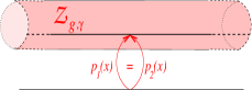
Figure 7: Conformal welding of a cylinder

${\cal Z}_{g,\gamma}\hskip 0.71114pt$ is isomorphic to the standard cylinder $\,{\cal Z}_{g_{0},\gamma}\hskip 0.71114pt$ for $\,g_{0}(x)\equiv x$,  with the isomorphism given by a function $\,{\cal X}:{\cal B}_{g,\gamma}\rightarrow\mathbb{C}\,$ holomorphic in the interior such that its boundary values $\,{\cal X}_{i}={\cal X}\circ p_{i}\,$ satisfy the relation

$${\cal X}_{1}(x)={\cal X}_{2}(x)-\mathrm{i}\gamma\,.$$ (7.28)

One may obtain such a function $\,{\cal X}\,$ by conformal welding of discs ShM . To this end, let us first consider the map

$${\cal B}_{g,\gamma}\ni z\,\longmapsto\,u={\rm e}^{\frac{2\pi}{\gamma}z}$$ (7.29)

that sends $\,{\cal B}_{g,\gamma}\,$ onto $\,\mathbb{C}\,$ cut along $\,\mathbb{R}_{+}\subset\mathbb{C}$,  with the sides of the cut parameterized by

$$\mathbb{R}\ni x\,\longmapsto\,{\rm e}^{\frac{2\pi}{\gamma}g(x)}+\mathrm{i}0\equiv\widetilde{p}_{1}(x)\qquad\text{and}\qquad\mathbb{R}\ni x\,\longmapsto\,{\rm e}^{\frac{2\pi}{\gamma}x}-\mathrm{i}0\equiv\widetilde{p}_{2}(x)\,.$$ (7.30)

Note that $\,\widetilde{p}_{1}(x)\,$ and $\,\widetilde{p}_{2}(x)\,$ agree for $\,|x|\,$ large enough. Welding the sides of the cut by identifying $\,\widetilde{p}_{1}(x)=\widetilde{p}_{2}(x)\,$ and adding the point $\,u=\infty$,  we obtain a closed Riemann surface $\,{\cal S}_{g}\,$ of genus zero. Another way to describe the same surface may be obtained using the map

$$\,u\,\longmapsto\,\frac{{1-\mathrm{i}u}}{{1+\mathrm{i}u}}$$ (7.31)

of $\,\mathbb{C}\cup\{\infty\}\cong\mathbb{C}P^{1}\,$ into itself that sends the real line $\,\mathbb{R}\,$ to the unit circle $\,S^{1}\,$ and $\,\mathbb{R}_{+}\subset\mathbb{R}\,$ into the lower half of the circle. Then $\,S_{g}\,$ may be viewed as obtained from the two discs into which the unit circle cuts $\,\mathbb{C}\cup\{\infty\}\,$ by welding them back together after twist by a circle diffeomorphism equal to the identity on a neighborhood of the upper half of the circle. As discussed  e.g. in ShM , one may construct an isomorphism of the surface $\,S_{g}\,$ obtained this way with $\,\mathbb{C}\cup\{\infty\}\,$ by solving an explicit Fredholm equation in $\,L^{2}(S^{1})$.  Composing that isomorphism with the map (7.31),  one obtains a holomorphic map $\,{\cal W}\,$ from $\,\mathbb{C}\setminus\mathbb{R}_{+}\,$ to $\,\mathbb{C}\cup\{\infty\}\,$ whose boundary values satisfy the relation

$${\cal W}(\widetilde{p}_{1}(x))={\cal W}(\widetilde{p}_{2}(x))$$ (7.32)

implying that $\,{\cal W}\,$ is also holomorphic in neighborhoods of $\,u=0\,$ and $\,u=\infty$. By composing $\,{\cal W}\,$ with an appropriate Möbius transformation, we may also demand that $\,{\cal W}(0)=0\,$ and $\,{\cal W}(\infty)=\infty\,$ so that

$${\cal W}(u)=\begin{cases}au+O(u^{2})\qquad\text{\,for}\qquad|u|\,\ \text{small}\,,\cr bu+O(1)\ \ \qquad\,\text{for}\qquad|u|\,\ \text{large}\end{cases}$$ (7.33)

for $\,a,b\not=0$.  Then the map

$${\cal B}_{\gamma,g}\ni z\,\longmapsto\,{\cal X}(z)\,=\,\frac{{}_{\gamma}}{{}^{2\pi}}\ln{{\cal W}({\rm e}^{\frac{2\pi}{\gamma}z})}\hskip 0.71114pt,$$ (7.34)

where $\,\ln(w)\,$ is chosen with a branch-cut along the image of $\,\mathbb{R}_{+}\,$ by $\,{\cal W}$,  is holomorphic in the interior of $\,{\cal B}_{g,\gamma}\,$ and its boundary values satisfy the relation (7.28) so that $\,{\cal X}\,$ defines the isomorphism $\,{\cal Z}_{g,\gamma}\cong{\cal Z}_{g_{0},\gamma}$.  In particular, from (7.33) we infer that

$${\cal X}_{i}^{\prime}(x)=\frac{\gamma}{{2\pi}}\,\frac{{\cal W}^{\prime}(\widetilde{p}_{i}(x))}{{\cal W}(\widetilde{p}_{i}(x))}\hskip 0.71114pt{\widetilde{p}_{i}}^{\hskip 0.56917pt\prime}(x)\,=\,\begin{cases}\,1+O({\rm e}^{\frac{2\pi}{\gamma}x})\qquad\ \,\text{for}\ \quad x\ll 0\hskip 0.71114pt,\cr\,1+O({\rm e}^{-\frac{2\pi}{\gamma}x})\qquad\text{for}\ \quad x\gg 0\hskip 0.71114pt.\end{cases}$$ (7.35)

Besides, $\,{\cal X}^{\prime}_{i}(x)\not=0$.  Writing

$${\cal X}_{1}(x)=g(x)-{\cal Y}_{1}(x)-\mathrm{i}\gamma\hskip 0.71114pt,\qquad{\cal X}_{2}(x)=x-{\cal Y}_{2}(x)={\cal X}_{1}(x)+\mathrm{i}\gamma\hskip 0.71114pt,$$ (7.36)

so that

$${\cal Y}_{12}(x)={\cal Y}_{1}(x)-{\cal Y}_{2}(x)=g(x)-x\hskip 0.71114pt,$$ (7.37)

we infer from (7.35) that $\,{\cal Y}^{\prime}_{i}(x)\,$ have an exponential decay when $\,x\to\pm\infty$.  Note that $\,{\cal Y}_{i}\,$ are the boundary values for the function $\,{\cal Y}(z)=z-{\cal X}(z)$.

It is easy to obtain an integral equation for $\,{\cal Y}_{1}\,$ similar to (6.29) of Sec. C. Indeed, using the Cauchy formula,

$${\cal Y}(z)=\frac{{}_{1}}{{}^{2\pi\mathrm{i}}}\int\frac{g^{\prime}(y)}{g(y)-\mathrm{i}\gamma-z}\,{\cal Y}_{1}(y)\,dy-\frac{{}_{1}}{{}^{2\pi\mathrm{i}}}\int\frac{1}{y-z}\,{\cal Y}_{2}(y)\,dy$$ (7.38)

for $\,z\,$ in the interior of $\,{\cal B}_{g,\gamma}\,$ and sending $\,z\,$ to $\,p_{i}(x)$,  one obtains the relations

$$\frac{{}_{1}}{{}^{2}}{\cal Y}_{1}(x)=\frac{{}_{1}}{{}^{2\pi\mathrm{i}}}\,PV\int\frac{g^{\prime}(y)}{g(y)-g(x)}\,{\cal Y}_{1}(y)\,dy-\frac{{}_{1}}{{}^{2\pi\mathrm{i}}}\int\frac{1}{y-g(x)+\mathrm{i}\gamma}\,{\cal Y}_{2}(y)\,dy\,,$$ (7.39)

$$\frac{{}_{1}}{{}^{2}}{\cal Y}_{2}(x)=\frac{{}_{1}}{{}^{2\pi\mathrm{i}}}\int\frac{g^{\prime}(y)}{g(y)-\mathrm{i}\gamma-x}\,{\cal Y}_{1}(y)\,dy-\frac{{}_{1}}{{}^{2\pi\mathrm{i}}}\,PV\int\frac{1}{y-x}\,{\cal Y}_{2}(y)\,dy$$ (7.40)

that, with the help of the identity

$$\frac{{}_{1}}{{}^{2}}\big{(}({\cal E}_{+}-{\cal E}_{-}){\cal X}\big{)}(x)=-\frac{{}_{1}}{{}^{2\pi\mathrm{i}}}\,PV\int\frac{1}{y-x}\,{\cal X}(y)\,dy\,,$$ (7.41)

where $\,{\cal E}_{\pm}\,$ are the orthogonal projections on functions $\,{\cal X}\in L^{2}(\mathbb{R})\,$ with the Fourier transform

$$\widehat{\cal X}(p)=\int{\rm e}^{\mathrm{i}px}\hskip 0.71114pt{\cal X}(x)\,dx$$ (7.42)

vanishing outside $\,\mathbb{R}_{\pm}$, respectively, may be rewritten in the form

$${\cal E}_{+}{\cal Y}_{1}={\cal K}_{11}{\cal Y}_{1}+{\cal K}_{12}{\cal Y}_{2}\,,\qquad{\cal E}_{-}{\cal Y}_{2}={\cal K}_{21}{\cal Y}_{1}\,,$$ (7.43)

for

$$({\cal K}_{11}{\cal X})(x)=\frac{{}_{1}}{{}^{2\pi\mathrm{i}}}\int\Big{(}\frac{g^{\prime}(y)}{g(y)-g(x)}-\frac{1}{y-x}\Big{)}{\cal X}(y)\,dy\hskip 0.71114pt,$$ (7.44)

$$({\cal K}_{12}{\cal X})(x)=-\frac{{}_{1}}{{}^{2\pi\mathrm{i}}}\int\frac{1}{y-g(x)+\mathrm{i}\gamma}\,{\cal X}(y)\,dy\hskip 0.71114pt,$$ (7.45)

$$({\cal K}_{21}{\cal X})(x)=\frac{{}_{1}}{{}^{2\pi\mathrm{i}}}\int\frac{g^{\prime}(y)}{g(y)-x-\mathrm{i}\gamma}\,{\cal X}(y)\,dy\hskip 0.71114pt.$$ (7.46)

The summation of (7.43) gives then rise to the integral equation

$$({\cal I}-{\cal K}){\cal Y}_{1}=({\cal E}_{-}-{\cal K}_{12}){\cal Y}_{12}\,,$$ (7.47)

where $\,{\cal I}\,$ stands for the identity operator in $\,L^{2}({\mathbb{R}})\,$ and

$${\cal K}={\cal K}_{11}+{\cal K}_{12}+{\cal K}_{21}\,.$$ (7.48)

We also have the representations:

$${\cal K}_{11}=-{\cal E}_{-}+{\cal G}^{-1}{\cal E}_{-}{\cal G}={\cal E}_{+}-{\cal G}^{-1}{\cal E}_{+}{\cal G}\,,\qquad{\cal K}_{12}={\cal G}^{-1}{\cal Q}\hskip 0.71114pt{\cal E}_{+}\,,\qquad{\cal K}_{21}={\cal E}_{-}{\cal Q}^{-1}{\cal G}\,,$$ (7.49)

where $\,({\cal G}{\cal X})(x)={\cal X}(g^{-1}(x))\,$ and $\,{\cal Q}\,{\rm e}^{-\mathrm{i}px}={\rm e}^{-\gamma p}\,{\rm e}^{-\mathrm{i}px}$. Contrary to the operator $\,K\,$ of Sec. C, the operator $\,{\cal K}\,$ in $\,L^{2}({\mathbb{R}})\,$ is not trace-class and the solution of Eq. (7.47) will require more care.

Note that for $\,f=f_{s,t,L}\,$ and $\,\tau=\tau_{s,L}\,$ the kernels of the operators $\,K_{ij}\,$ of  (6.24)-(6.26)  become

$$K_{11}(x,y)=-\frac{1}{L}\Big{(}\frac{g^{\prime}_{s,t,L}(y)}{1-{\rm e}^{\frac{2\pi\mathrm{i}}{L}(g_{s,t,L}(y)-g_{s,t,L}(x))}}-\frac{1}{1-{\rm e}^{-\frac{2\pi\mathrm{i}}{L}(x-y)}}\Big{)}\,$$ (7.50)

$$K_{12}(x,y)=\frac{1}{L\Big{(}1-{\rm e}^{\frac{2\pi\mathrm{i}}{L}(y-g_{s,t,L}(x)+\mathrm{i}\gamma_{L})}\Big{)}}\,,$$ (7.51)

$$K_{21}(x,y)=-\frac{g^{\prime}_{s,t,L}(y)}{L\Big{(}1-{\rm e}^{\frac{2\pi\mathrm{i}}{L}(g_{s,t,L}(y)-x-\mathrm{i}\gamma_{L})}\Big{)}}\,,$$ (7.52)

where $\,g_{s,t,L}\,$ are given by (7.16). From the results of Sec. A it follows that in the frames centered at $\,O^{\pm}_{L}\,$ of (7.7) and (7.18) they converge pointwise to the kernels of operators $\,{\cal K}_{ij}\,$ for $\,g=g^{\pm}_{s,t}\,$ when $\,L\to\infty$.  This renders plausible the convergence of the derivatives of functions $\,X_{s,t,L;i}\,$ in the recentered frames to the derivatives of the functions $\,{\cal X}^{\pm}_{s,t;i}\,$ obtained from conformal welding of the cylinders $\,{\cal Z}_{g^{\pm}_{s,t},\gamma}$.  Indeed, the corresponding functions are determined in terms of the solution of, respectively, Eq. (6.29) and (7.47). A rigorous proof of such a convergence, however, requires more subtle analysis that will be presented in Sec. 9.

C Infinite-volume formula for the FCS generating function

We shall assume here the uniform convergence on compacts of derivatives of the functions $\,X_{s,t,L;i}\,$ occurring in (6.115) and (6.116) in the frames with centers at $\,O_{L}^{\pm}\,$ to derivatives of functions $\,{\cal X}^{\pm}_{s,t;i}\,$ obtained from conformal welding of cylinders $\,{\cal Z}_{g^{\pm}_{s,t},\gamma}$,  in agreement with the discussion of the last subsection. For the first term on the right-hand side of (6.115),  we obtain then the limiting behavior

$$\lim\limits_{L\to\infty}\,\exp\bigg{[}-\mathrm{i}\,\frac{{}_{c}}{{}^{24\pi}}\int_{0}^{\frac{\lambda}{\Delta\beta}}ds\int_{{\cal I}_{L}}\xi_{t,L}(x)(SX_{s,t,L;i})(x)\,dx\bigg{]}$$ (7.53)

$$=\,\exp\bigg{[}-\mathrm{i}\,\frac{{}_{c}}{{}^{24\pi}}\sum\limits_{\pm}\int_{0}^{\frac{\lambda}{\Delta\beta}}ds\int\xi^{\pm}_{t}(x)(S{\cal X}^{\pm}_{s,t;i})(x)\,dx\bigg{]}.\quad$$ (7.54)

We are still left with the control of the $\,L\to\infty\,$ limit of the ratio of Virasoro characters in (6.115). Note that $\,\tau_{0,L}=\mathrm{i}\hskip 0.71114ptL^{-1}\gamma_{L}=O(L^{-1})\,$ and that $\,\widehat{\tau}_{\frac{\lambda}{\Delta\beta},t,L}-\tau_{0,L}=O(L^{-2})\,$ as follows from (6.116) and the relation

$$\lim\limits_{L\to\infty}\,\int_{0}^{\frac{\lambda}{\Delta\beta}}ds\hskip 0.85355pt\int_{{\cal I}_{L}}\xi_{t,L}(x)\,(X^{\prime}_{s,t,L;i}(x))^{2}\,dx\,=\,\sum\limits_{\pm}\int_{0}^{\frac{\lambda}{\Delta\beta}}ds\int\xi^{\pm}_{t}(x)\,({{\cal X}^{\pm}_{s,t;i}}^{\prime}\hskip 3.98337pt(x))^{2}\,dx\,.$$ (7.55)

The behavior when $\,\tau\to 0\,$ for the Virasoro character $\,\chi(\tau)\,$ of the finite-volume theory may be obtained from the dual picture or the modular properties of the characters of of the Virasoro algebra or its extensions:

$$\chi(\tau)=C\,{\rm e}^{2\pi\mathrm{i}\frac{c}{24\tau}}\big{(}1+o(e^{-\frac{\epsilon}{|\tau|}})\big{)},$$ (7.56)

where $\,C>0\,$ and $\,\epsilon>0\,$ are constants dependent on the theory but independent of $\,\tau$.  This holds e.g. for general rational unitary CFTs where $\,\chi(\tau)\,$ is a finite sum of the characters of a chiral algebra transforming linearly under $\,\tau\mapsto-\frac{1}{\tau}\,$ DFMS ,  but also for toroidal compactifications of free fields, e.g. for the massless bosonic field considered in Sec. B with any radius of compactification. Assuming (7.56), we infer that

$$\lim\limits_{L\to\infty}\,\frac{\chi(\widehat{\tau}_{\frac{\lambda}{\Delta\beta},t,L})}{\chi(\tau_{0,L})}\,=\,\exp\Big{[}-\mathrm{i}\frac{{}_{\pi c}}{{}^{12}}\,\lim\limits_{L\to\infty}\frac{{}_{\widehat{\tau}_{\frac{\lambda}{\Delta\beta},t,L}-\,\hskip 0.71114pt\tau_{0,L}}}{{}^{\tau_{0,L}^{2}}}\Big{]}$$ (7.57)

$$=\,\exp\Big{[}\mathrm{i}\hskip 0.71114pt\frac{{}_{\pi c}}{{}^{12\gamma^{2}}}\,\sum\limits_{\pm}\int_{0}^{\frac{\lambda}{\Delta\beta}}ds\int\xi^{\pm}_{t}(x)\,({{\cal X}^{\pm}_{s,t;i}}^{\prime}\hskip 3.41418pt(x))^{2}\,dx\Big{]},$$ (7.58)

where, as before, $\,\gamma=v\beta_{0}$.  Collecting (7.54), (7.58) and (7.3), we obtain for the infinite-volume generating function for FCS of energy transfers the expression

$$\Psi_{t}(\lambda)\,\equiv\,\lim\limits_{L\to\infty}\,\Psi_{t,L}(\lambda)\,=\,\prod\limits_{\pm}\Psi_{t}^{\pm}(\lambda)\,,$$ (7.59)

where $\,\Psi^{\pm}_{t}(\lambda)\,$ are the contributions of the right- and left-movers,  respectively,  given by the relations

$$\Psi^{\pm}_{t}(\lambda)\,=\,\exp\bigg{[}-\mathrm{i}\,\frac{{}_{c}}{{}^{24\pi}}\,\bigg{(}\int_{0}^{\frac{\lambda}{\Delta\beta}}ds\int\xi^{\pm}_{t}(x)\hskip 0.71114pt\Big{(}(S{\cal X}^{\pm}_{s,t;i})(x)-\frac{{}_{2\pi^{2}}}{{}^{\gamma^{2}}}\,({{\cal X}^{\pm}}^{\prime}_{s,t;i}(x))^{2}\Big{)}\hskip 0.71114ptdx$$ (7.60)

$$\hskip 157.91287pt+\,\frac{{}_{\lambda\hskip 0.28436ptv}}{{}^{\Delta\beta}}\int\big{(}\beta(x^{\pm})-\beta(x)\big{)}\,(Sh)(x)\,dx\bigg{)}\bigg{]}.$$ (7.61)

The last formulae show that in the infinite-volume, the generating function $\,\Psi_{t}(\lambda)\,$ for the FCS of energy transfers in the non-equilibrium profile states is universal depending only on the profile $\,\beta(x)\,$ and the central charge $\,c\,$ of the CFT but not on the spectrum of the theory. Besides, the central charge enters simply as an overall power.

D Simple checks: the first two moments of the energy transfer

In virtue of (5.12), the average energy transfer through the kink is given in the infinite-volume limit by the expression

$$\langle\Delta E\rangle^{\ }_{\hskip 0.28436ptt}=\lim\limits_{L\to\infty}\,\langle\Delta E\rangle^{\ }_{t,L}=\lim\limits_{L\to\infty}\,\frac{{}_{1}}{{}^{\Delta\beta}}\big{\langle}G_{L}(t)-G_{L}(0)\big{\rangle}^{\rm neq}_{\,L}$$ (7.62)

$$=\frac{{}_{v}}{{}^{\Delta\beta}}\int\Big{(}(\beta(x^{+})-\beta(x))\big{\langle}T_{+}(x)\big{\rangle}^{\rm neq}+(\beta(x^{-})-\beta(x))\big{\langle}T_{-}(x)\big{\rangle}^{\rm neq}\Big{)}dx$$ (7.63)

$$=\frac{{}_{v}}{{}^{\Delta\beta}}\int\Big{(}(\beta(x^{+})-\beta(x))\big{(}\frac{{}_{\pi c}}{{}^{12(v\beta(x))^{2}}}-\frac{{}_{c}}{{}^{24\pi}}(Sh)(x)\big{)}\,+\,(\beta(x^{-})-\beta(x))\big{(}\frac{{}_{\pi c}}{{}^{12(v\beta(x))^{2}}}-\frac{{}_{c}}{{}^{24\pi}}(Sh)(x)\big{)}\Big{)}dx$$ (7.64)

$$=\frac{{}_{\pi c}}{{}^{12\gamma^{2}\Delta\beta}}\sum\limits_{\pm}\int\xi^{\pm}_{t}(y)\,dy\,-\frac{{}_{cv}}{{}^{24\pi\Delta\beta}}\sum\limits_{\pm}\int\Big{(}\beta(x^{\pm})-\beta(x)\Big{)}(Sh)(x)\,dx\,,\qquad$$ (7.65)

where we have used (4.49), (7.12) and (7.19),  changing the integration variable to $\,y=h(x)\,$ in the part of the integral. The result agrees with $\,\frac{{}_{1}}{{}^{\mathrm{i}}}\,\partial_{\lambda}\hskip 0.71114pt\ln{\Psi_{t}(0)}\,$ for $\,\Psi_{y}(\lambda)\,$ given by (7.59) and (7.61) since $\,{{\cal X}^{\pm}}^{\prime}_{0,t;i}(x)=1$.

For the variance of the energy transfer given by (5.13), we obtain in the infinite-volume limit the expression

$$\big{\langle}\Delta E;\Delta E\big{\rangle}^{c}_{t}=\lim\limits_{L\to\infty}\,\big{\langle}\Delta E;\Delta E\big{\rangle}^{c}_{t,L}=\lim\limits_{L\to\infty}\,\frac{{}_{1}}{{{}^{(\Delta\beta)^{2}}}}\Big{\langle}G_{L}(t)-G_{L}(0)\,;\,G_{L}(t)-G_{L}(0)\Big{\rangle}^{\rm neq,\,c}_{L}$$ (7.66)

$$=\frac{{}_{v^{2}}}{{}^{(\Delta\beta)^{2}}}\int\Big{(}\big{(}\beta(x_{1}^{+})-\beta(x_{1})\big{)}\big{(}\beta(x_{2}^{+})-\beta(x_{2})\big{)}\Big{\langle}T_{+}(x_{1})\,;\,T_{+}(x_{2})\Big{\rangle}^{{\rm neq},\,c}$$ (7.67)

$$\hskip 48.36958pt+\,\big{(}\beta(x_{1}^{-})-\beta(x_{1})\big{)}\big{(}\beta(x_{2}^{-})-\beta(x_{2})\big{)}\Big{\langle}T_{-}(x_{1})\,;\,T_{-}(x_{2})\Big{\rangle}^{{\rm neq},\,c}\,\Big{)}\hskip 0.71114ptdx_{1}dx_{2}$$ (7.68)

$$=\frac{{}_{\pi^{2}c}}{{}^{8(\Delta\beta)^{2}\gamma^{4}}}\sum\limits_{\pm}\int\bigg{(}\frac{\xi^{\pm}_{t}(y_{1})\,\xi^{\pm}_{t}(y_{2})}{\sinh^{4}\big{(}\frac{\pi}{\gamma}(y_{1}-y_{2}-\mathrm{i}0)\big{)}}\bigg{)}dy_{1}dy_{2}\,,$$ (7.69)

where we used (4.50), (4.51) and (7.12) and the way the singularity $\,\propto\frac{1}{(y_{1}-y_{2})^{4}}\,$ has been treated was obtained by writing

$$\Big{\langle}G_{L}(t)-G_{L}(0)\,;\,G_{L}(t)-G_{L}(0)\Big{\rangle}^{{\rm neq},\,c}_{\,L}$$ (7.70)

$$=\,\lim\limits_{\epsilon\searrow 0}\,\Big{\langle}G_{L}(t)-G_{L}(0)\,;\,{\rm e}^{-\epsilon G_{L}(0)}\big{(}G_{L}(t)-G_{L}(0)\big{)}\,{\rm e}^{\epsilon G_{L}(0)}\Big{\rangle}^{{\rm neq},\,c}_{L}.\ \quad$$ (7.71)

Expressing $\,\xi^{\pm}_{t}(y)\,$ by its Fourier transform,

$$\widehat{\xi^{\pm}_{t}}(p)=\int{\rm e}^{\mathrm{i}py}\,\xi^{\pm}_{t}(y)\,dy\,,$$ (7.72)

and using the result (B.12) from Appendix B, we infer that

$$\big{\langle}\Delta E;\Delta E\big{\rangle}^{c}_{t} = \frac{{}_{\pi^{2}c}}{{}^{8(\Delta\beta)^{2}\gamma^{4}}}\frac{{}_{1}}{{}^{(2\pi)^{2}}}\sum\limits_{\pm}\int\Big{(}\frac{{\rm e}^{-\mathrm{i}(p_{1}y_{1}+p_{2}y_{2})}}{\sinh^{4}\big{(}\frac{\pi}{\gamma}(y_{1}-y_{2}-\mathrm{i}0)\big{)}}\,\widehat{\xi^{\pm}_{t}}(p_{1})\,\widehat{\xi_{t}^{\pm}}(p_{2})\Big{)}\hskip 0.71114ptdp_{1}dp_{2}dy_{1}dy_{2}$$ (7.73)

$$= \frac{{}_{c}}{{}^{48\pi^{2}(\Delta\beta)^{2}}}\sum\limits_{\pm}\int\frac{p\big{(}p^{2}+\frac{{4\pi^{2}}}{{\gamma^{2}}}\big{)}}{1-{\rm e}^{-\gamma p}}\,\widehat{\xi^{\pm}_{t}}(p)\,\widehat{\xi^{\pm}_{t}}(-p)\,dp\,.$$ (7.74)

In order to compare this to $\,-\partial_{\lambda}^{2}\hskip 0.71114pt\ln{\Psi_{t}(0)}$,  we have to find the $\hskip 0.71114pt1^{\rm st}\,$ order correction in $\,s\,$ given by $\,\partial_{s}{{\cal X}^{\pm}}^{\prime}_{0,t;i}(x)\,$ to $\,{{\cal X}^{\pm}}^{\prime}_{0,t;i}=1$.  Write $\,{\cal X}^{\pm}_{s,t;1}(x)=g^{\pm}_{s,t}(x)-{\cal Y}_{s;1}(x)-\mathrm{i}\gamma$,  see (7.36), recalling that $\,{\cal Y}_{s;1}\,$ satisfies (7.47) for $\,g=g^{\pm}_{s,t}$.  Differentiating the latter equation with $\,{\cal Y}_{12}=g^{\pm}_{s,t}-g_{0}\,$ over $\,s\,$ at $\,s=0$,  where, as before, $\,g_{0}(x)=x$,  one gets:

$$(1-{\cal K}^{0})\partial_{s}{\cal Y}_{0;1}=({\cal E}_{-}-{\cal K}^{0}_{12})(-\xi^{\pm}_{t})$$ (7.75)

where $\,{\cal K}^{0}_{ij}\,$ correspond to $\,g=g_{0}$.  In terms of the Fourier transforms, (7.75) reads:

$$\big{(}1-{\rm e}^{-\gamma|p|}\big{)}\partial_{s}\widehat{{\cal Y}_{0;1}}(p)=-\big{(}\theta(-p)-{\rm e}^{-\gamma p}\theta(p)\big{)}\widehat{\xi}^{\pm}_{t}(p)$$ (7.76)

and we infer that

$$\partial_{s}{{\cal X}^{\pm}}^{\prime}_{0,t;1}(x)=-{\xi^{\pm}_{t}}^{\prime}(x)-\frac{{}_{\mathrm{i}}}{{}^{2\pi}}\int{\rm e}^{-\mathrm{i}px}\,\frac{p(\theta(-p)-{\rm e}^{-\gamma p}\theta(p))}{1-{\rm e}^{-\gamma|p|}}\,\widehat{\xi}^{\pm}_{t}(p)\,dp\,=\,\frac{{}_{\mathrm{i}}}{{}^{2\pi}}\int\frac{p\,{\rm e}^{-\mathrm{i}px}}{1-{\rm e}^{-\gamma p}}\,\widehat{\xi}^{\pm}_{t}(p)\,dp\,,$$ (7.77)

$$\partial_{s}(S{\cal X}^{\pm}_{0,t;1})(x)=\partial_{s}{{\cal X}^{\pm}}^{\prime\prime\prime}_{0,t;1}(x)=-\frac{{}_{\mathrm{i}}}{{}^{2\pi}}\int\frac{p^{3}\,{\rm e}^{-\mathrm{i}px}}{1-{\rm e}^{-\gamma p}}\,\widehat{\xi}^{\pm}_{t}(p)\,dp\,.$$ (7.78)

Hence

$$-\partial_{\lambda}^{2}\hskip 0.71114pt\ln{\Psi_{t}(0)}\,=\,\mathrm{i}\,\frac{{}_{c}}{{}^{24\pi(\Delta\beta)^{2}}}\sum\limits_{\pm}\int\xi^{\pm}_{t}(x)\Big{(}\partial_{s}(S{\cal X}^{\pm}_{0,t;1})(x)-\frac{{}_{4\pi^{2}}}{{}^{\gamma^{2}}}{{\cal X}^{\pm}}^{\prime}_{0,t;1}(x)\hskip 0.71114pt\partial_{s}{{\cal X}^{\pm}}^{\prime}_{0,t;1}(x)\Big{)}\,dx$$ (7.79)

$$=\,\frac{{}_{c}}{{}^{48\pi^{2}(\Delta\beta)^{2}}}\sum\limits_{\pm}\int\xi^{\pm}_{t}(x)\Big{(}\int\frac{p\hskip 0.71114pt(p^{2}+\frac{4\pi^{2}}{\gamma^{2}})\,{\rm e}^{-\mathrm{i}px}}{1-{\rm e}^{-\gamma p}}\,\widehat{\xi}^{\pm}_{t}(p)\,dp\Big{)}\,dx$$ (7.80)

$$=\,\frac{{}_{c}}{{}^{48\pi^{2}(\Delta\beta)^{2}}}\sum\limits_{\pm}\int\frac{p\big{(}p^{2}+\frac{{4\pi^{2}}}{{\gamma^{2}}}\big{)}}{1-{\rm e}^{-\gamma p}}\,\widehat{\xi}^{\pm}_{t}(p)\,\widehat{\xi}^{\pm}_{t}(-p)\,dp$$ (7.81)

which agrees with (7.74).

8 Long-time behavior of FCS

It is not difficult to understand heuristically the long-time large-deviations type asymptotics of the right-hand side of (7.61). Using the relations (7.14) and (7.23), we observe that the functions $\,\xi^{\pm}_{t}\hskip 0.71114pt$ are, respectively, equal to constant values $\,\gamma\frac{\Delta\beta}{\beta_{\cal L}}\,$ and $\,-\gamma\frac{\Delta\beta}{\beta_{\cal R}}\,$ for $\,\gamma=v\beta_{0}\,$ on intervals of length $\,\frac{\gamma}{\beta_{\cal L}}t-O(1)\,$ and $\,\frac{\gamma}{\beta_{\cal R}}t-O(1)$,  and that they vanish outside $\,O(1)\,$ extensions of those intervals.  It follows that the shifted flows $\,g_{s,t}^{\pm}(x)=f_{s,t}^{\pm}(x)+\gamma s$, which satisfy the equations

$$\partial_{s}g^{\pm}_{s,t}(x)=-\xi^{\pm}_{t}(g^{\pm}_{s,t}(x)-\gamma s)\,,\qquad g^{\pm}_{0,t}(x)=x\,,$$ (8.1)

are equal, respectively, to $\,x-\gamma\frac{\Delta\beta}{\beta_{\cal L}}s\equiv\widetilde{g}^{+}_{s}(x)\,$ and to $\,x+\gamma\frac{\Delta\beta}{\beta_{\cal R}}s\equiv\widetilde{g}^{-}_{s}(x)\,$ on those intervals shortened by $\,O(|s|)\,$ on either side.  For estimating the right-hand side of (7.61), we would like to know the behavior of the functions $\,{{\cal X}^{\pm}}^{\prime}_{s,t;i}\,$ on the support of $\,\xi^{\pm}_{t}$.  In the bulk of the support, we expect $\,{{\cal X}^{\pm}}^{\prime}_{s,t;i}(x)\,$ to fast approach for large $\,t\,$ the functions obtained from conformal welding of the cylinders $\,{\cal Z}_{\widetilde{g}^{\pm}_{s},\gamma}$. The holomorphic maps $\,\widetilde{\cal X}^{\pm}_{s}:{\cal B}_{\widetilde{g}^{\pm}_{s},\gamma}\rightarrow\mathbb{C}\,$ generating the isomorphisms $\,{\cal Z}_{\widetilde{g}^{\pm}_{s},\gamma}\cong{\cal Z}_{g_{0},\gamma}\,$ are in that case given simply by the multiplication by complex factors:

$$\widetilde{\cal X}^{+}_{s}(z)=\big{(}1-\mathrm{i}\frac{{}_{\Delta\beta}}{{}^{\beta_{\cal L}}}s\big{)}^{-1}z+C^{+}\,,\qquad\widetilde{\cal X}^{-}_{s}(z)=\big{(}1+\mathrm{i}\frac{{}_{\Delta\beta}}{{}^{\beta_{\cal R}}}s\big{)}^{-1}z+C^{-}$$ (8.2)

up to arbitrary additive constants $\,C^{\pm}$.  Indeed,

$$\widetilde{\cal X}^{+}_{s;1}(x) = \widetilde{\cal X}^{+}_{s}(-\mathrm{i}\gamma+\widetilde{g}^{+}_{s}(x))=\big{(}1-\mathrm{i}\frac{{}_{\Delta\beta}}{{}^{\beta_{\cal L}}}s\big{)}^{-1}\big{(}-\mathrm{i}\gamma+x-\gamma\frac{{}_{\Delta\beta}}{{}^{\beta_{\cal L}}}s\big{)}+C^{+}$$ (8.3)

$$= \big{(}1-\mathrm{i}\frac{{}_{\Delta\beta}}{{}^{\beta_{\cal L}}}s\big{)}^{-1}x+C^{+}-\mathrm{i}\gamma=\widetilde{\cal X}^{+}_{s;2}(x)-\mathrm{i}\gamma\,,$$ (8.4)

$$\widetilde{\cal X}^{-}_{s;1}(x) = \widetilde{\cal X}^{-}_{s}(-\mathrm{i}\gamma+\widetilde{g}^{-}_{s}(x))=\big{(}1+\mathrm{i}\frac{{}_{\Delta\beta}}{{}^{\beta_{\cal R}}}s\big{)}^{-1}\big{(}-\mathrm{i}\gamma+x+\gamma\frac{{}_{\Delta\beta}}{{}^{\beta_{\cal R}}}s\big{)}+C^{-}$$ (8.5)

$$= \big{(}1+\mathrm{i}\frac{{}_{\Delta\beta}}{{}^{\beta_{\cal R}}}s\big{)}^{-1}x+C^{-}-\mathrm{i}\gamma=\widetilde{\cal X}^{-}_{s;2}(x)-\mathrm{i}\gamma$$ (8.6)

so that

$${\widetilde{\cal X}^{+}_{s;i}}{}^{\prime}(x)=\big{(}1-\mathrm{i}\frac{{}_{\Delta\beta}}{{}^{\beta_{\cal L}}}s\big{)}^{-1}\,,\qquad{\widetilde{\cal X}^{-}_{s;i}}{}^{\prime}(x)=\big{(}1+\mathrm{i}\frac{{}_{\Delta\beta}}{{}^{\beta_{\cal R}}}s\big{)}^{-1}\,.$$ (8.7)

A rigorous proof of the convergence of the derivatives of functions $\,{{\cal X}^{\pm}}_{s,t;i}\,$ to those of $\,{\widetilde{\cal X}^{\pm}}_{s;i}(x)\,$ in the bulk of the support of $\,\xi^{\pm}_{t}\,$ requires a rather subtle control of the solutions of the Fredholm equation that computes $\,{{\cal X}^{\pm}}_{s,t;i}\,$ that we have not performed in detail. Assuming such a convergence, the only contributions to the large-deviations rates

$$\Xi^{\pm}(\lambda)\,=\,\lim\limits_{t\to\infty}\,\frac{1}{t}\,\ln{\Psi^{\pm}_{t}(\lambda)}$$ (8.8)

would come from the middle terms on the right-hand side of (7.61) leading to the formulae

$$\Xi^{+}(\lambda)\,=\,\mathrm{i}\frac{{}_{\pi c}}{{}^{12\gamma^{2}}}\int_{0}^{\frac{\lambda}{\Delta\beta}}\frac{{}_{\gamma}}{{}^{\beta_{\cal L}}}\gamma\frac{{}_{\Delta\beta}}{{}^{\beta_{\cal L}}}\big{(}1-\mathrm{i}\frac{{}_{\Delta\beta}}{{}^{\beta_{\cal L}}}s\big{)}^{-2}\hskip 0.71114ptds\,=\,\frac{{}_{\pi c}}{{}^{12}}\Big{(}\frac{{}_{1}}{{}^{\beta_{\cal L}-\mathrm{i}\lambda}}-\frac{{}_{1}}{{}^{\beta_{\cal L}}}\Big{)},$$ (8.9)

$$\Xi^{-}(\lambda)\,=\,\mathrm{i}\frac{{}_{\pi c}}{{}^{12\gamma^{2}}}\int_{0}^{\frac{\lambda}{\Delta\beta}}\frac{{}_{\gamma}}{{}^{\beta_{\cal R}}}(-\gamma)\frac{{}_{\Delta\beta}}{{}^{\beta_{\cal R}}}\big{(}1+\mathrm{i}\frac{{}_{\Delta\beta}}{{}^{\beta_{\cal R}}}s\big{)}^{-2}\hskip 0.71114ptds\,=\,\frac{{}_{\pi c}}{{}^{12}}\Big{(}\frac{{}_{1}}{{}^{\beta_{\cal R}+\mathrm{i}\lambda}}-\frac{{}_{1}}{{}^{\beta_{\cal R}}}\Big{)},$$ (8.10)

in agreement with the Bernard-Doyon result BD0 obtained for the partitioning protocol. For $\,c=1$,  the latter expressions also agree with the large-volume long-time limit of the Levitov-Lesovik formula for two channels of free massless fermions with pure transmission that gives LL2 ; LLL ; MBHD

$$\sum\limits_{\pm}\Xi^{\pm}(\lambda)=\frac{{}_{1}}{{}^{2\pi}}\int\ln\Big{[}1+f_{\cal L}(\omega)(1-f_{\cal R}(\omega))({\rm e}^{\mathrm{i}\lambda\omega}-1)+f_{{\cal R}}(\omega)(1-f_{{\cal L}}(\omega))({\rm e}^{-\mathrm{i}\lambda\omega}-1)\Big{]}\hskip 0.71114ptd\omega\hskip 0.71114pt,$$ (8.11)

where $\,f_{\cal L}(\omega)=\frac{1}{{{\rm e}^{\beta_{\cal L}\omega}+1}}\,$ and $\,f_{\cal R}(\omega)=\frac{1}{{{\rm e}^{\beta_{\cal R}\omega}+1}}\,$ are the Fermi functions for the right and left movers. Observe that the functions $\,\Xi^{\pm}(\lambda)\,$ depend on the inverse-temperature profile only via its asymptotic values $\,\beta_{\cal L},\beta_{\cal R}\,$ exhibiting even more universality than $\,\Psi_{t}^{\pm}(\lambda)$.  The Legendre transform

$${\cal I}(\sigma)\,=\mathop{{\rm sup}}\limits_{\nu\in]-\beta_{\cal R},\beta_{\cal L}[}\Big{(}\nu\sigma\,-\,\frac{{}_{\pi c}}{{}^{12}}\Big{(}\frac{{}_{\nu}}{{}^{\beta_{\cal L}(\beta_{\cal L}-\nu)}}-\frac{{}_{\nu}}{{}^{\beta_{\cal R}(\beta_{\cal R}+\nu)}}\Big{)}\Big{)}$$ (8.12)

with the asymptotic behavior

$${\cal I}(\sigma)=\begin{cases}\ \beta_{\cal L}\sigma-\sqrt{\frac{\pi c}{3}\sigma}\,+\,O(1)\quad\hskip 13.08846pt\text{when}\quad\sigma\to\infty\cr-\beta_{\cal R}\sigma-\sqrt{-\frac{\pi c}{3}\sigma}\,+\,O(1)\quad\text{when}\quad\sigma\to-\infty\end{cases}$$ (8.13)

determines the long-time large-deviations form of the of energy transfers in the thermodynamic limit:

$$P_{t}(\Delta E)\,=\,\lim\limits_{L\to\infty}\,P_{t,L}(\Delta E)\ \ {{}_{\begin{subarray}{c}{}_{\smile}\\ {}^{\frown}\end{subarray}}}\ \,\exp\big{[}-t\hskip 0.85355pt{\cal I}\big{(}\frac{{}_{\Delta E}}{{}^{t}}\big{)}\big{]}.$$ (8.14)

The rate function possesses the Gallavotti-Cohen symmetry GalCoh : $\,{\cal I}(-\sigma)={\cal I}(\sigma)+\sigma\Delta\beta\,$ that follows here from the transient fluctuation relation (5.19).

Another way to characterize the behavior of the FCS at large times is to note that

$$t\hskip 0.71114pt\frac{{}_{\pi c}}{{}^{12}}\Big{(}\frac{{}_{\mathrm{i}\lambda}}{{}^{\beta_{\cal L}(\beta_{\cal L}-\mathrm{i}\lambda)}}-\frac{{}_{\mathrm{i}\lambda}}{{}^{\beta_{\cal R}(\beta_{\cal R}+\mathrm{i}\lambda)}}\Big{)}=\,t\frac{{}_{\pi c}}{{}^{12}}\int({\rm e}^{\mathrm{i}\lambda q}-1)\Big{(}{\rm e}^{-\beta_{\cal L}q}\theta(q)+{\rm e}^{\beta_{\cal R}q}\theta(-q)\Big{)}dq$$ (8.15)

is the logarithm of the Fourier transform of the time-$t\,$ distribution of a Lévy process Lawler with the jump rates

$$w(x,y)=\frac{{}_{\pi c}}{{}^{12}}\Big{(}{\rm e}^{-\beta_{\cal L}(y-x)}\theta(y-x)+{\rm e}^{-\beta_{\cal R}(x-y)}\theta(x-y)\Big{)}$$ (8.16)

that starts at $\,x=0$.  The right hand side of (8.15) gives the Lévy-Khintchine representation for the infinitely divisible distribution of such a process, see also BD0 ; BD2 .

9 Thermodynamic limit of FCS:  proof of convergence

This section fills the missing element in the proof that the thermodynamic limit of the FCS generating function $\,\Psi_{t,L}(\lambda)\,$ given by (6.115) and (6.116) takes the form (7.59)-(7.61). It is addressed to readers not convinced by the heuristic arguments of Sec. 7.

The functions $\,X_{s,t,L;i}\,$ that appear in (6.115) and (6.116) satisfy the relations

$$X_{s,t,L;1}=g_{s,t,L}-Y_{1}-L\tau_{0,L}\,,\quad X_{s,t,L;2}=X_{s,t,L;1}+L\widehat{\tau}_{s,t,L}\,,$$ (9.1)

where $\,Y_{1}\,$ is the solution of the Fredholm equation (6.29) related to conformal welding of tori described in Sec. C. On the other hand, the functions $\,{\cal X}^{\pm}_{s,t;i}\,$ that appear in the formula (7.61) satisfy the relations

$${\cal X}^{\pm}_{s,t;1}(x)=g^{+}_{s,t}(x)-{\cal Y}^{\pm}_{1}(x)-\mathrm{i}\gamma\,,\qquad{\cal X}^{\pm}_{s,t;2}(x)={\cal X}^{\pm}_{s,t;1}+\mathrm{i}\gamma\,,$$ (9.2)

where $\,{\cal Y}^{\pm}_{1}\,$ are solutions of Eq. (7.47) for $\,g=g^{\pm}_{s,t}\,$ obtained in the context of conformal welding of cylinders discussed in Sec. B.

We shall prove here the uniform convergence on compacts with all derivatives of the functions $\,X^{\prime}_{s,t,L;1}\,$ viewed in the frames centered at $\,O^{\pm}_{L}\,$ of (7.7) and (7.18) to the functions $\,X^{\pm}_{s,t;i}{}^{\prime}\ \,$. We often suppress the dependence on $\,(s,t,L)\,$ in the notation for the finite-volume quantities (like for $\,Y_{1}\,$ in (9.1)) and on $\,(s,t)\,$ in the infinite volume (like for $\,{\cal Y}^{\pm}_{1}\,$ in (9.2)). All the estimates established below are uniform in $\,s=\frac{\lambda}{\Delta\beta}\,$ belonging to bounded sets.

A Recasting equation for $\,Y_{1}$

The main point is to control the behavior for large $\,L\,$ of the derivatives of functions $\,Y_{1}\,$ solving Eq. (6.29) in the frames centered at $\,O^{\pm}_{L}$. To this end, it will be convenient to rewrite the Fredholm equation (6.29) in which $\,K=K_{11}+K_{12}+K_{21}\,$ with

$$K_{11}=E_{0+}-G^{-1}E_{0+}G=-E_{-}+G^{-1}E_{-}G\hskip 0.71114pt,\qquad K_{12}=G^{-1}QE_{0+}\hskip 0.71114pt,\qquad K_{21}=E_{-}Q^{-1}G$$ (9.3)

for $\,(G^{-1}X)(x)=X(g_{s,t,L}(x))\,$ and $\,Q\hskip 0.71114pte_{n}={\rm e}^{-\frac{2\pi n}{L}\gamma_{L}}e_{n}$,  see (6.27),  and where

$$Y_{12}(x)=g_{s,t,L}(x)-x+L(\widehat{\tau}_{s,t,L}-\tau_{0,L})\,.$$ (9.4)

First, we shall eliminate from (6.29) the constant mode contributions involving the toroidal modular parameters. Applying the orthogonal projector $\,E^{\perp}_{0}=E_{+}+E_{-}\,$ to the both sides of (6.29), we obtain the relation

$$E_{0}^{\perp}(I-K)Y_{1}=E_{0}^{\perp}(I-K)E_{0}^{\perp}Y_{1}=E_{0}^{\perp}(E_{-}-K_{12})(E_{0}^{\perp}Y_{12}+E_{0}Y_{12})=E_{0}^{\perp}(E_{-}-K_{12})E_{0}^{\perp}Y_{12}$$ (9.5)

since $\,E_{0}^{\perp}K_{ij}E_{0}=0$. Recall that the kernel of $\,I-K\,$ is composed of constants, the range of $\,I-K\,$ has codimension 1, and the solvability of (6.29) fixes uniquely the constant contribution to $\,Y_{12}$,  see (6.31), with $\,E_{-}-K_{12}\,$ mapping constants into constants. Thus the range of $\,I-K\,$ cannot contain nonzero constants. It follows that the operator $\,E_{0}^{\perp}(I-K)E_{0}^{\perp}\,$ is invertible on the range of $\,E_{0}^{\perp}\,$ and that the function $\,E_{0}^{\perp}Y_{1}\,$ is uniquely determined by (9.5) from $\,E_{0}^{\perp}Y_{12}$.  Note from (9.3) that $\,K^{0}=QE_{0+}+E_{-}Q^{-1}\,$ is the operator $\,K\,$ for $\,g_{s,t,L}\,$ replaced by the identity diffeomorphism. Explicitly, $\,K^{0}e_{n}={\rm e}^{-\frac{2\pi|n|}{L}\gamma_{L}}e_{n}$.  Factoring out the part related to $\,K^{0}$,  we shall rewrite

$$E_{0}^{\perp}(I-K)E_{0}^{\perp}=E_{0}^{\perp}\Big{(}I-(K-K^{0})E_{0}^{\perp}\big{(}E_{0}^{\perp}(I-K^{0})E_{0}^{\perp}\big{)}^{-1}\Big{)}E_{0}^{\perp}(I-K^{0})E_{0}^{\perp}\hskip 0.71114pt,$$ (9.6)

where

$$K-K^{0} = -E_{-}+G^{-1}E_{-}G+(G^{-1}-I)QE_{0+}+E_{-}Q^{-1}(G-I)$$ (9.7)

$$= E_{0+}-G^{-1}E_{0+}G+(G^{-1}-I)QE_{0+}+E_{-}Q^{-1}(G-I)\hskip 0.71114pt.$$ (9.9)

In the matrix notation corresponding to the decomposition $\,L^{2}_{0}(S^{1}_{L})\equiv E_{0}^{\perp}L^{2}(S^{1}_{L})=E_{+}L^{2}(S^{1}_{L})\oplus E_{-}L^{2}(S^{1}_{L})$,

$$E_{0}^{\perp}(I-K)E_{0}^{\perp}\,=\,\left(\begin{matrix}E_{+}+\Sigma_{++}&\ \Sigma_{+-}\cr\Sigma_{-+}&\ E_{-}+\Sigma_{--}\end{matrix}\right)\left(\begin{matrix}(I-Q)_{++}&\ 0\cr 0&\ (I-Q^{-1})_{--}\end{matrix}\right),$$ (9.10)

where

$$\Sigma_{++}=-\Big{(}(G^{-1})_{+-}G_{-+}+\big{(}(G^{-1}-I)Q\big{)}_{++}\Big{)}(I-Q)_{++}^{\,-1}\,,$$ (9.11)

(9.12)

$$\Sigma_{+-}=(G^{-1})_{++}G_{+-}(I-Q^{-1})^{\,-1}_{--}\,,$$ (9.13)

(9.14)

$$\Sigma_{-+}=-\Big{(}(G^{-1})_{--}G_{-+}+(G^{-1}Q)_{-+}+(Q^{-1}G)_{-+}\Big{)}(I-Q)_{++}^{\,-1}\,,$$ (9.15)

(9.16)

$$\Sigma_{--}=\Big{(}(G^{-1})_{-+}G_{+-}-\big{(}Q^{-1}(G-I)\big{)}_{--}\Big{)}(I-Q^{-1})^{\,-1}_{--}$$ (9.17)

in the notation $\,D_{++}\equiv E_{+}DE_{+}$, $\,D_{+-}\equiv E_{+}DE_{-}$,  etc.  Similarly,

$$E_{0}^{\perp}(E_{-}-K_{12})E_{0}^{\perp}=\left(\begin{matrix}-(G^{-1}Q)_{++}&\ 0\cr-(G^{-1}Q)_{-+}&\ E_{-}\end{matrix}\right).$$ (9.18)

Hence (9.5) becomes

$$\left(\begin{matrix}E_{+}+\Sigma_{++}&\ \Sigma_{+-}\cr\Sigma_{-+}&\ E_{-}+\Sigma_{--}\end{matrix}\right)\left(\begin{matrix}Z_{+}\cr Z_{-}\end{matrix}\right)=\left(\begin{matrix}-(G^{-1}Q)_{++}Y_{12}\cr-(G^{-1}Q)_{-+}Y_{12}+E_{-}Y_{12}\end{matrix}\right).$$ (9.19)

for

$$Z=Z_{+}+Z_{-}=(I-K^{0})Y_{1}\qquad\text{or}\qquad Z_{+}=(I-Q)_{++}Y_{1}\,,\quad\ Z_{-}=(I-Q^{-1})_{--}Y_{1}\,.$$ (9.20)

Recall that $\,K\,$ is trace-class in $\,L^{2}(S^{1}_{L})\,$ so that from (9.10) it follows that the operator $\,\Sigma=\big{(}\begin{subarray}{c}\Sigma_{++}\,\Sigma_{+-}\\ \Sigma_{-+}\,\Sigma_{--}\end{subarray}\big{)}\,$ on $\,L^{2}_{0}(S^{1}_{L})\,$ is also trace-class and that $\,I+\Sigma\,$ is invertible on that space.

To control the $\,L\to\infty\,$ limit, we shall need a better control of those operators. Note that, for $\,L\,$ sufficiently large, the diffeomorphism $\,g_{s,t,L}\,$ is equal to the identity except on two disjoint intervals, one inside $]-\frac{1}{4}L,\frac{1}{4}L[\,$ and the other inside $]-\frac{3}{4}L,-\frac{1}{4}L[$.  Let us set

$$g^{+}_{s,t,L}(x)=\begin{cases}g_{s,t,L}(x+O^{+}_{L})-O^{+}_{L}\quad\text{for}\quad x+O^{+}_{L}\in]-\frac{1}{4}L,\frac{1}{4}L[\,,\cr\,x\qquad\text{otherwise}\,,\end{cases}$$ (9.21)

$$g^{-}_{s,t,L}(x)=\begin{cases}g_{s,t,L}(x+O^{-}_{L})-O^{-}_{L}\quad\text{for}\quad x+O^{-}_{L}\in]-\frac{3}{4}L,-\frac{1}{4}L[\,,\cr\,x\qquad\text{otherwise}\,,\end{cases}$$ (9.22)

so that

$$g_{s,t,L}(x+O^{+}_{L})-O^{+}_{L}-x=g^{+}_{s,t,L}(x)-x+g^{-}_{s,t,L}(x+M_{L})-M_{L}-x\,,$$ (9.23)

where $\,M_{L}\,$ is given by (7.24). When restricted to $\,{\cal I}_{L}$, $\,g^{\pm}_{s,t,L}\,$ may be viewed as diffeomorphisms of $\,S^{1}_{L}={\mathbb{R}}/L{\mathbb{Z}}\,$ and,  when considered on the whole line,  as diffeomorphisms of $\,{\mathbb{R}}$. In the latter case, it follows from the analysis of Sec. A that $\,g^{\pm}_{s,t,L}(x)=g^{\pm}_{s,t}(x)=x\,$ outside an $\hskip 0.71114ptL$-independent bounded set and that for $\,\ell=0,1,\dots$,

$$|\partial_{x}^{\ell}g^{\pm}_{s,t,L}(x)-\partial_{x}^{\ell}g^{\pm}_{s,t}(x)|\leq L^{-1}C_{\ell}$$ (9.24)

uniformly in $\,x$.

Let $\,T_{b}\,$ and $\,(G^{\pm})^{\mp 1}\,$ be the translation and substitution operators acting on $\,L^{2}(S^{1}_{L})\,$ by

$$(T_{b}X)(x)=X(x-b)\,,\qquad((G^{\pm})^{-1}X)(x)=X(g^{\pm}_{s,t,L}(x))\,.$$ (9.25)

Given an operator $\,D\,$ acting on $\,L^{2}(S^{1}_{L})$,  we shall denote by $\,\widetilde{D}\,$ the operator $\,T_{O^{+}_{L}}^{-1}D\,T_{O^{+}_{L}}$,  i.e. the operator $\,D\,$ viewed in the frame centered at $\,O^{+}_{L}$.  The relation (9.23) implies that

$${\widetilde{G}}^{-1}-I=(G^{+})^{-1}-I+T_{M_{L}}^{-1}((G^{-})^{-1}-I)\hskip 0.71114ptT_{M_{L}}$$ (9.26)

and,  similarly,

$$\widetilde{G}-I=G^{+}-I+T_{M_{L}}^{-1}(G^{-}-I)T_{M_{L}}\,.$$ (9.27)

Since $\,T_{b}\,$ commutes with $\,E_{\pm}$,  we infer that

$$({\widetilde{G}}^{\mp 1}-I)_{++}=((G^{+})^{\mp 1}-I)_{++}+T_{M_{L}}^{-1}((G^{-})^{\mp 1}-I)_{++}\hskip 0.71114ptT_{M_{L}}\,,$$ (9.28)

$$({\widetilde{G}}^{\mp 1}-I)_{--}=((G^{+})^{\mp 1}-I)_{--}+T_{M_{L}}^{-1}((G^{-})^{\mp 1}-I)_{--}\hskip 0.71114ptT_{M_{L}}\,,$$ (9.29)

$$({\widetilde{G}}^{\mp 1})_{+-}=((G^{+})^{\mp 1})_{+-}+T_{M_{L}}^{-1}((G^{-})^{\mp 1})_{+-}\hskip 0.71114ptT_{M_{L}}\,,$$ (9.30)

$$({\widetilde{G}}^{\mp 1})_{-+}=((G^{+})^{\mp 1})_{-+}+T_{M_{L}}^{-1}((G^{-})^{\mp 1})_{-+}\hskip 0.71114ptT_{M_{L}}\,.$$ (9.31)

In the frame centered at $\,O^{+}_{L}$, the relation (9.19) becomes

$$(I+\widetilde{\Sigma})\widetilde{Z}=-\Big{(}({\widetilde{G}}^{-1}Q)_{++}+({\widetilde{G}}^{-1}Q)_{-+}-E_{-}\Big{)}\widetilde{Y}_{12}\,,$$ (9.32)

where

$$\widetilde{Z}=T_{O^{+}_{L}}^{-1}Z\,,\qquad\widetilde{Y}_{12}=T_{O^{+}_{L}}^{-1}Y_{12}$$ (9.33)

and,  by (9.4) and (9.23),  we may take

$$\widetilde{Y}_{12}=Y^{+}_{12}+T_{M_{L}}^{-1}Y^{-}_{12}$$ (9.34)

for

$$Y^{+}_{12}=g^{+}_{s,t,L}-g_{0}\,,\qquad Y^{-}_{12}=g^{-}_{s,t,L}-g_{0}$$ (9.35)

dropping constant terms from $\,Y_{12}\,$ that do not change the right hand side of (9.32). The operator $\,\widetilde{\Sigma}=T_{O^{+}_{L}}^{-1}\Sigma\hskip 0.71114ptT_{O^{+}_{L}}\,$ on $\,L^{2}_{0}(S^{1}_{L})\,$ is obtained from the relations (9.11)-(9.17) by replacing $\,G^{\pm 1}\,$ by $\,\widetilde{G}^{\pm 1}$.

We have to deal with the fact that the contribution of the right- and left-movers corresponding to diffeomorphisms $\,g^{\pm}_{s,t,L}\,$ are mixed together in finite volume. Let $\,\Sigma^{+}\,$ be the operator obtained from $\,\widetilde{\Sigma}\,$ by replacing all inputs with $\,\widetilde{G}^{\mp 1}\,$ by the first terms on the right-hand side of (9.28)-(9.31) and let $\,T_{M_{L}}^{-1}\Sigma^{-}T_{M_{L}}\,$ be obtained similarly but using the second terms on the right-hand side of (9.28)-(9.31). Consider first the decoupled equations

$$(I+{\Sigma}^{\pm})Z^{\pm}=-\Big{(}((G^{\pm})^{-1}Q)_{++}+((G^{\pm})^{-1}Q)_{-+}-E_{-}\Big{)}Y^{\pm}_{12}\hskip 0.71114pt.$$ (9.36)

They may be solved for $\,Z^{\pm}\,$ because $\,I+\Sigma^{\pm}$,  similarly as $\,I+\Sigma$,  are invertible on $\,L^{2}_{0}(S^{1}_{L})$.  Exhibiting the corrections due to the coupling between the right- and left-movers, we shall write

$$\widetilde{\Sigma}\,=\,\Sigma^{+}+T_{M_{L}}^{-1}\Sigma^{-}T_{M_{L}}+\delta\widetilde{\Sigma}\,,$$ (9.37)

where

$$\delta\widetilde{\Sigma}_{++}=-\Big{(}((G^{+})^{-1})_{+-}T_{M_{L}}^{-1}(G^{-})_{-+}T_{M_{L}}+T_{M_{L}}^{-1}((G^{-})^{-1})_{+-}T_{M_{L}}(G^{+})_{-+}\Big{)}(I-Q)_{++}^{\,-1}\,,$$ (9.38)

(9.39)

$$\delta\widetilde{\Sigma}_{+-}=\Big{(}((G^{+})^{-1}-I)_{++}T_{M_{L}}^{-1}(G^{-})_{+-}T_{M_{L}}+T_{M_{L}}^{-1}((G^{-})^{-1}-I)_{++}T_{M_{L}}(G^{+})_{+-}\Big{)}(I-Q^{-1})^{\,-1}_{--}\,,\quad$$ (9.40)

(9.41)

$$\delta\widetilde{\Sigma}_{-+}=-\Big{(}((G^{+})^{-1}-I)_{--}T_{M_{L}}^{-1}(G^{-})_{-+}T_{M_{L}}+T_{M_{L}}^{-1}((G^{-})^{-1}-I)_{--}T_{M_{L}}(G^{+})_{-+}\Big{)}(I-Q)_{++}^{\,-1}\,,$$ (9.42)

(9.43)

$$\delta\widetilde{\Sigma}_{--}=\Big{(}((G^{+})^{-1})_{-+}T_{M_{L}}^{-1}(G^{-})_{+-}T_{M_{L}}+T_{M_{L}}^{-1}((G^{-})^{-1})_{-+}T_{M_{L}}(G^{+})_{+-}\Big{)}(I-Q^{-1})_{--}^{\,-1}\,.$$ (9.44)

and

$$\widetilde{Z}\,=\,Z^{+}+T_{M_{L}}^{-1}Z^{-}+\delta\widetilde{Z}\,.$$ (9.45)

The decoupled contributions (9.36) to (9.32) will now cancel out resulting in the equation

$$\big{(}I+\widetilde{\Sigma}\big{)}\delta\widetilde{Z} = -\Big{(}T_{M_{L}}^{-1}\Sigma^{-}T_{M_{L}}+\delta\widetilde{\Sigma}\Big{)}Z^{+}-\Big{(}\Sigma^{+}+\delta\widetilde{\Sigma}\Big{)}T_{M_{L}}^{-1}Z^{-}$$ (9.48)

$$-\Big{(}T_{M_{L}}^{-1}(((G^{-})^{-1}-I)Q)_{++}T_{M_{L}}+T_{M_{L}}^{-1}((G^{-})^{-1}Q)_{-+}T_{M_{L}}\Big{)}Y^{+}_{12}$$

$$-\Big{(}(((G^{+})^{-1}-I)Q)_{++}+((G^{+})^{-1}Q)_{-+}\Big{)}T_{M_{L}}^{-1}Y^{-}_{12}$$

for $\,\delta\widetilde{Z}$.  Below, we shall show that this equation implies that $\,\delta\widetilde{Z}\,$ tends to zero in an appropriate sense when $\,L\to\infty$. This will establish the factorization of the right- and left-movers contributions in the thermodynamic limit.

Following similar steps as in finite volume,  the infinite-volume equation (7.47) with $\,g=g^{\pm}_{s,t}\,$ may be recast upon writing

$${\cal I}-{\cal K}=\big{(}{\cal I}-({\cal K}-{\cal K}^{0})({\cal I}-{\cal K}^{0})^{-1}\big{)}({\cal I}-{\cal K}^{0})$$ (9.49)

into the form

$$({\cal I}+\varSigma^{\pm}){\cal Z}^{\pm}=-\Big{(}(({\cal G}^{\pm})^{-1}{\cal Q})_{++}\hskip 0.71114pt+(({\cal G}^{\pm})^{-1}{\cal Q})_{-+}\hskip 0.71114pt-{\cal E}_{-}\Big{)}{\cal Y}^{\pm}_{12}$$ (9.50)

where $\hskip 0.71114pt\,\varSigma^{\pm}=\big{(}\begin{matrix}{}_{\varSigma^{\pm}_{++}}&{}_{\varSigma^{\pm}_{+-}}\cr{}^{\varSigma^{\pm}_{-+}}&{}^{\varSigma^{\pm}_{--}}\end{matrix}\big{)}\,\hskip 0.71114pt$ act in $\,L^{2}({\mathbb{R}})={\cal E}_{+}L^{2}({\mathbb{R}})\oplus{\cal E}_{-}L^{2}({\mathbb{R}})\,$ and have the components $\,\varSigma_{++}={\cal E}_{+}\varSigma\hskip 0.71114pt{\cal E}_{+}$,  etc.,  given by Eqs. (9.11)-(9.17) in which $\,G^{\pm 1}\,$ is replaced by the operators $\,({\cal G}^{\pm})^{\pm 1}\,$ such that $\,(({\cal G}^{\pm})^{-1}{\cal X})(x)={\cal X}(g^{\pm}_{s,t}(x))$,  and where

$${\cal Z}^{\pm}=({\cal I}-{\cal K}^{0}){\cal Y}^{\pm}_{1}\,,\qquad{\cal Y}^{\pm}_{12}=g^{\pm}_{s,t}-g_{0}\,.$$ (9.51)

Above, $\,{\cal K}^{0}={\cal Q}\hskip 0.71114pt{\cal E}_{+}+{\cal E}_{-}{\cal Q}^{-1}\,$ denotes the operator $\,{\cal K}\,$ of (7.48) for $\,g\,$ equal to the identity diffeomorphism $\,g_{0}$.

B Fast-decay and Schwartz type operators

We shall consider operators on $\,L^{2}({\mathbb{R}})\,$ acting in the momentum space representation by

$$(\widehat{{\cal D}{\cal X}})(p)\,=\,\frac{{}_{1}}{{}^{2\pi}}\int\widehat{\cal D}(p,q)\,\widehat{\cal X}(q)\,dq\,dx\hskip 0.71114pt.$$ (9.52)

for $\,\widehat{X}(p)\,$ given by (7.42).

Definition 1.  We shall call $\,{\cal D}\,$ of fast-decay type if for any $\,k=0,1,\dots\,$ there exists a constant $\,C_{k}\,$ such that

$$|\widehat{\cal D}(p,q)|\leq\frac{C_{k}}{(1+p^{2})^{k}(1+q^{2})^{k}}\,.$$ (9.53)

Let $\,\widehat{\cal J},\,\widehat{\cal J}^{\prime}\,$ be open subsets of $\,\mathbb{R}$. We shall call $\,{\cal D}\,$ of Schwartz $\widehat{\cal J}\times\widehat{\cal J}^{\prime}$ type if $\,(i)$ $\,\widehat{\cal D}(p,q)=0\,$ for $\,(p,q)\notin\widehat{\cal J}\times\widehat{\cal J}^{\prime}$, $\,(ii)$ $\,\widehat{\cal D}(p,q)\,$ is smooth on $\widehat{\cal J}\times\widehat{\cal J}^{\prime}$, and  $(iii)$ for any $\,\ell_{1},\ell_{2},k=0,1,\dots\,$ there exists a constant $\,C_{\ell_{1},\ell_{2},k}\,$ such that

$$|\partial_{p}^{\ell_{1}}\partial_{q}^{\ell_{2}}\widehat{\cal D}(p,q)|\leq\frac{C_{\ell_{1},\ell_{2},k}}{(1+p^{2})^{k}(1+q^{2})^{k}}$$ (9.54)

on $\,\widehat{\cal J}\times\widehat{\cal J}^{\prime}$,

Definition 2.  Let $\,{\cal D}_{L},\,{\cal D}\,$ be operators of fast-decay type. We shall say that $\,{\cal D}_{L}\,$ converge to $\,{\cal D}\,$ with speed $\,L^{-1}\,$ if for any $\,k=0,1,\dots\,$ there exists a constant $\,C_{k}\,$ such that

$$|\widehat{\cal D}_{L}(p,q)-\widehat{\cal D}(p,q)|\leq\frac{L^{-1}C_{k}}{(1+p^{2})^{k}(1+q^{2})^{k}}$$ (9.55)

for all $\,L\geq L_{0}\,$ where $\,L_{0}\,$ is $\,k$-independent. Similarly, the convergence with speed $\,L^{-1}\,$ of Schwartz $\widehat{\cal J}\times\widehat{\cal J}^{\prime}$ type operators is defined by demanding that for any $\,\ell_{1},\ell_{2},k=0,1,\dots\,$ there exists a constant $\,C_{\ell_{1},\ell_{2},k}\,$ such that

$$\big{|}\partial_{p}^{\ell_{1}}\partial_{q}^{\ell_{2}}\big{(}\widehat{\cal D}_{L}(p,q)-\widehat{\cal D}(p,q)\big{)}\big{|}\leq\frac{L^{-1}C_{\ell_{1},\ell_{2},k}}{(1+p^{2})^{k}(1+q^{2})^{k}}$$ (9.56)

on $\,\widehat{\cal J}\times\widehat{\cal J}^{\prime}\,$ for all $\,L\geq L_{0}$.

Note that the Schwartz-type operators are of fast decay type,  that the latter are Hilbert-Schmidt Simon ,  and that the Schwartz-type convergence implies the fast-decay one.

Definition 3. We shall call a function $\,X\in L^{2}_{0}(S^{1}_{L})\,$ the $L$-periodization of a function $\,{\cal X}\,$ on $\,{\mathbb{R}}\,$ if $\,\sqrt{L}\,\big{\langle}e_{n}\big{|}X\big{\rangle}=\widehat{\cal X}(p_{n})\,$ for $\,0\not=n\in{\mathbb{Z}}$,  where $\,e_{n}(x)=\frac{1}{\sqrt{L}}{\rm e}^{-\mathrm{i}p_{n}x}\,$ and $\,p_{n}\equiv\frac{2\pi n}{L}$.  Similarly, we shall call an operator $\,D\,$ on $\,L^{2}_{0}(S^{1}_{L})\,$ with the matrix elements $\,D_{mn}=\langle e_{m}|D|e_{n}\rangle\,$ the $L$-periodization of an operator $\,{\cal D}\,$ on $\,L^{2}({\mathbb{R}})\,$ with momentum-space kernel $\,\widehat{{\cal D}}(p,q)\,$ if $\,L\hskip 0.71114ptD_{mn}=\widehat{{\cal D}}(p_{m},p_{n})\,$ for $\,0\not=m,n\in{\mathbb{Z}}$.

Definition 4. We shall call an operator $\,D\,$ on $\,L^{2}_{0}(S^{1}_{L})\,$ of fast-decay or Schwartz $\,\widehat{\cal J}\times\widehat{\cal J}^{\prime}\,$ type if $\,D\,$ is the $L$-periodization of an operator $\,{\cal D}\,$ on $\,L^{2}({\mathbb{R}})\,$ of the corresponding type. If $\,D_{L}\,$ are the $L$-periodization of fast-decay or Schwartz $\widehat{\cal J}\times\widehat{\cal J}^{\prime}$ type operators $\,{\cal D}_{L}\,$ on $\,L^{2}({\mathbb{R}})\,$ converging as such to operator $\,{\cal D}\,$ with speed $\,L^{-1}$,  we shall say that $\,D_{L}\,$ converge to $\,{\cal D}\,$ with speed $\,L^{-1}\,$ as fast-decay or Schwartz $\widehat{\cal J}\times\widehat{\cal J}^{\prime}$ type operators.

In Appendix C we present basic general results about the fast-decay and Schwartz type operators and the related Fredholm operators, their determinants and their inverses that we shall frequently evoke in the sequel.

C Schwartz-type convergence results

Let $\,g:\mathbb{R}\rightarrow\mathbb{R}\,$ be a diffeomorphism that is equal to the identity outside a bounded subset of $\,\mathbb{R}\,$ and let $\,{\cal G}\,$ be the substitution operator on $\,L^{2}(\mathbb{R})$,

$$({\cal G}^{-1}{\cal X})(x)={\cal X}(g(x))\hskip 0.71114pt.$$ (9.57)

We shall denote by $\,{\cal P}\,$ the operator $\,\mathrm{i}\partial_{x}\,$ and by $\,{\cal Q}\,$ the operator $\,{\rm e}^{-\gamma_{\#}{\cal P}}\,$ for $\,\gamma_{\#}=\gamma_{L}\,$ or $\,\gamma_{\#}=\gamma$,  as specified below,  with $\,\gamma_{L}=v\beta_{0,L}\,$ and $\,\gamma=v\beta_{0}$.  As before, $\,{\cal E}_{\pm}\,$ will denote the orthogonal projections in $\,L^{2}(\mathbb{R})\,$ on functions with Fourier transform vanishing outside $\,\mathbb{R}_{\pm}\,$ and we shall use the shorthand notation $\,{\cal D}_{++}={\cal E}_{+}{\cal D}\hskip 0.71114pt{\cal E}_{+}$,  etc.

Lemma 2.  The following operators on $\,L^{2}(\mathbb{R})\,$ are of Schwartz ${\mathbb{R}}_{\sigma}\times{\mathbb{R}}_{\sigma^{\prime}}$ type:

• $\,{\cal D}_{1}=({\cal G}^{-1}{\cal P}^{-1})_{+-}=(({\cal G}^{-1}-{\cal I}){\cal P}^{-1})_{+-}\,$  for $\,(\sigma,\sigma^{\prime})=(+,-)$ ,

• $\,{\cal D}_{2}=({\cal G}^{-1}{\cal P}^{-1})_{-+}=(({\cal G}^{-1}-{\cal I}){\cal P}^{-1})_{-+}\,$  for $\,(\sigma,\sigma^{\prime})=(-,+)$ ,

• $\,{\cal D}_{3}=(({\cal G}^{-1}-{\cal I}){\cal Q}{\cal P}^{-1})_{++}\,$                     for $\,(\sigma,\sigma^{\prime})=(+,+)$ ,

• $\,{\cal D}_{4}=({\cal Q}^{-1}({\cal G}^{-1}-{\cal I}){\cal P}^{-1})_{--}\,$                  for $\,(\sigma,\sigma^{\prime})=(-,-)$ ,

• $\,{\cal D}_{5}=({\cal G}^{-1}-{\cal I})_{++}({\cal G}{\cal P}^{-1})_{+-}\,$                  for $\,(\sigma,\sigma^{\prime})=(+,-)$ ,

• $\,{\cal D}_{6}=({\cal G}^{-1}-{\cal I})_{--}({\cal G}{\cal P}^{-1})_{-+}\,$                  for $\,(\sigma,\sigma^{\prime})=(-,+)$ ,

The same claims hold for the above operators with $\,{\cal G}\,$ and $\,{\cal G}^{-1}\,$ interchanged.

The proof of Lemma 2 based on straightforward estimates is given in Appendix D. Applying Lemma 2 to the case when $\,g=g^{\pm}_{s,t,L}\,$ of (9.21) and (9.22) with $\,{\cal Q}={\rm e}^{-\gamma_{L}{\cal P}}\,$ or  to $\,g=g_{s,t}^{\pm}\,$ with $\,{\cal Q}={\rm e}^{-\gamma{\cal P}}$,  we infer that the corresponding operators $\,{\cal D}^{\pm}_{i,L}\,$ and $\,{\cal D}^{\pm}_{i}\,$ for $\,i=1,\dots,6\,$ are of Schwartz type. A straightforward modification of the proof of Lemma 2, see Appendix D, together with the estimates (9.24), show that $\,{\cal D}^{\pm}_{i,L}\,$ converge to $\,{\cal D}^{\pm}_{i}\,$ with speed $\,L^{-1}\,$ as operators of Schwartz-type.  For $\,i=5,6$,  we introduce an additional modification of $\,{\cal D}^{\pm}_{i,L}$,  described at the end of the proof of Lemma 2 in Appendix D, which does not change the above properties. Now, let $\,D^{\pm}_{i,L}\,$ be the $L$-periodization of the operators $\,{\cal D}^{\pm}_{i,L}$.  In view of Definition 4, the operators $\,D^{\pm}_{i,L}\,$ converge with speed $\,L^{-1}\hskip 0.71114pt$ to $\,{\cal D}^{\pm}_{i}\,$ as operators of Schwartz type. Explicitly, $\,D^{\pm}_{i,L}\,$ are the operators

$$D^{\pm}_{1,L}=((G^{\pm})^{-1}P^{-1})_{+-}\,,\hskip 65.44142ptD_{2,L}^{\pm}=((G^{\pm})^{-1}P^{-1})_{-+}\,,$$ (9.58)

$$D^{\pm}_{3,L}=((G^{\pm})^{-1}-I)_{++}(QP^{-1})_{++}\,,\qquad D^{\pm}_{4,L}=(Q^{-1})_{--}((G^{\pm})^{-1}-I)_{--}(P^{-1})_{--}\,,$$ (9.59)

$$D^{\pm}_{5,L}=((G^{\pm})^{-1}-I)_{++}(G^{\pm}P^{-1})_{+-}\,,\hskip 13.6572ptD^{\pm}_{6,L}=((G^{\pm})^{-1}-I)_{--}(G^{\pm}P^{-1})_{-+}\,,$$ (9.60)

where $\,P{\rm e}_{n}=p_{n}{\rm e}_{n}\,$ and $\,(G^{\pm})^{-1}\,$ are the operators of substitution of $\,g^{\pm}_{s,t,L}\,$ acting on $\,L^{2}_{0}(S^{1}_{L})$.  On the other hand,

$${\cal D}^{\pm}_{1}=(({\cal G}^{\pm})^{-1}{\cal P}^{-1})_{+-}\,,\hskip 66.57933pt\quad{\cal D}^{\pm}_{2}=(({\cal G}^{\pm})^{-1}{\cal P}^{-1})_{-+}\,,$$ (9.61)

$${\cal D}^{\pm}_{3}=(({\cal G}^{\pm})^{-1}-{\cal I})_{++}({\cal Q}{\cal P}^{-1})_{++}\,,\qquad\quad{\cal D}^{\pm}_{4}=({\cal Q}^{-1})_{--}(({\cal G}^{\pm})^{-1}-{\cal I})_{--}({\cal P}^{-1})_{--}\,,$$ (9.62)

$${\cal D}^{\pm}_{5}=(({\cal G}^{\pm})^{-1}-{\cal I})_{++}({\cal G}^{\pm}{\cal P}^{-1})_{+-}\,,\hskip 25.6073pt{\cal D}^{\pm}_{6}=(({\cal G}^{\pm})^{-1}-{\cal I})_{--}({\cal G}^{\pm}{\cal P}^{-1})_{-+}\,,$$ (9.63)

where $\,({\cal G}^{\pm})^{-1}\,$ are the operator of substitution of $\,g^{\pm}_{s,t}\,$ acting on $\,L^{2}({\mathbb{R}})$.

Recall from Sec. A that the operators $\hskip 0.71114pt\,\Sigma^{\pm}=\big{(}\begin{matrix}{}_{\Sigma^{\pm}_{++}}&{}_{\Sigma^{\pm}_{+-}}\cr{}^{\Sigma^{\pm}_{-+}}&{}^{\Sigma^{\pm}_{--}}\end{matrix}\big{)}\,\hskip 0.71114pt$ on $\,L^{2}_{0}(S^{1}_{L})\,$ have the components that are given by Eqs. (9.11)-(9.17) with $\,G^{\pm 1}\,$ replaced by $\,(G^{\pm})^{\pm 1}\,$ and that their $\,L=\infty\,$ version acting in $\,L^{2}({\mathbb{R}})\,$ are the operators $\hskip 0.71114pt\,\varSigma^{\pm}=\big{(}\begin{matrix}{}_{\varSigma^{\pm}_{++}}&{}_{\varSigma^{\pm}_{+-}}\cr{}^{\varSigma^{\pm}_{-+}}&{}^{\varSigma^{\pm}_{--}}\end{matrix}\big{)}\,\hskip 0.71114pt$ with the components given by Eqs. (9.11)-(9.17) in which $\,G^{\pm 1}\,$ is replaced by $\,({\cal G}^{\pm})^{\pm 1}\,$ and $\,Q\,$ by $\,{\cal Q}={\rm e}^{-\gamma{\cal P}}$. Let $\,{\mathbb{R}}_{\not=0}={\mathbb{R}}\setminus\{0\}$.

Proposition 1.  The operators $\,\Sigma^{\pm}\,$ and $\,\varSigma^{\pm}\,$ are of Schwartz ${\mathbb{R}}_{\not=0}\times{\mathbb{R}}_{\not=0}$ type and $\,\Sigma^{\pm}\,$ converge with speed $\,L^{-1}\hskip 0.71114pt$ to $\,\varSigma^{\pm}\,$ as such.

Remark.  Schwartz ${\mathbb{R}}_{\not=0}\times{\mathbb{R}}_{\not=0}$ type operators have momentum-space kernels that are smooth away from $\,\{0\}\times{\mathbb{R}}\cup{\mathbb{R}}\times\{0\}\,$ but may be discontinuous across that set.

Proof of Proposition 1.  The claim follows from the above results and their version with diffeomorphisms $\,g^{\pm}_{s,t,L}\,$ and $\,g^{\pm}_{s,t}\,$ replaced by their inverses,  together with Propositions C2 and C3 of Appendix C. For example, in

$$\Sigma^{\pm}_{++}=-\Big{(}\big{(}G^{\pm})^{-1}\big{)}_{+-}G^{\pm}_{-+}+\big{(}((G^{\pm})^{-1}-I)Q\big{)}_{++}\Big{)}(I-Q)^{-1}_{++}\,,$$ (9.64)

the operators $\,\big{(}(G^{\pm})^{-1}\big{)}_{+-}G^{\pm}_{-+}(I-Q)^{-1}_{++}\,$ are the $L$-periodization of $\,{\cal D}^{\pm}_{1,L}{\cal P}\hskip 0.71114pt{\cal D}^{\pm}_{2,L}\big{(}\frac{{\cal P}}{{\cal I}-{\rm e}^{-\gamma_{L}{\cal P}}}\big{)}_{{++}}$,  where in $\,{\cal D}^{\pm}_{2,L}\,$ one should invert $\,g^{\pm}_{s,t,L}$.  Those operators converge with speed $\,L^{-1}\,$ as operators of Schwartz ${\mathbb{R}}_{+}\times{\mathbb{R}}_{+}$ type to $\,{\cal D}^{\pm}_{1}{\cal P}\hskip 0.71114pt{\cal D}^{\pm}_{2}\big{(}\frac{{\cal P}}{{\cal I}-{\rm e}^{-\gamma{\cal P}}}\big{)}_{++}$,  where in $\,{\cal D}^{\pm}_{2}\,$ one should invert $\,g^{\pm}_{s,t,}$.  Similarly, $\,\big{(}((G^{\pm})^{-1}-I)Q\big{)}_{++}(I-Q)^{-1}_{++}\,$ is the $L$-periodization of $\,{\cal D}^{\pm}_{3,L}\big{(}\frac{{\cal P}}{{\cal I}-{\rm e}^{-\gamma_{L}{\cal P}}}\big{)}_{++}\,$ that converges to $\,{\cal D}^{\pm}_{3}\big{(}\frac{{\cal P}}{{\cal I}-{\rm e}^{-\gamma{\cal P}}}\big{)}_{++}$.  In

$$\Sigma^{\pm}_{-+}=-\Big{(}\big{(}(G^{\pm})^{-1}-I\big{)}_{--}G^{\pm}_{-+}+G^{\pm}_{-+}+\big{(}(G^{\pm})^{-1}Q\big{)}_{-+}+\big{(}Q^{-1}G^{\pm}\big{)}_{-+}\Big{)}(I-Q)^{-1}_{++}\,,$$ (9.65)

the operators $\,\big{(}(G^{\pm})^{-1}-I\big{)}_{--}G^{\pm}_{-+}(I-Q)^{-1}_{++}\,$ are the $L$-periodization of $\,{\cal D}^{\pm}_{6,L}\big{(}\frac{{\cal P}}{I-{\rm e}^{-\gamma_{L}{\cal P}}}\big{)}_{++}$. They converge with speed $\,L^{-1}\,$ to $\,{\cal D}^{\pm}_{6}\big{(}\frac{{\cal P}}{I-{\rm e}^{-\gamma{\cal P}}}\big{)}_{++}\,$ as operators of Schwartz ${\mathbb{R}}_{-}\times{\mathbb{R}}_{+}$ type. Similarly, $\,G^{\pm}_{-+}(I-Q)^{-1}_{++}\,$ are the $L$-periodization of $\,{\cal D}^{\pm}_{2,L}\big{(}\frac{{\cal P}}{{\cal I}-{\rm e}^{-\gamma_{L}{\cal P}}}\big{)}_{++}$,  where in $\,{\cal D}_{2,L}^{\pm}\,$ one should invert $\,g^{\pm}_{s,t,L}$. They converge to $\,{\cal D}^{\pm}_{2}\big{(}\frac{{\cal P}}{{\cal I}-{\rm e}^{-\gamma{\cal P}}}\big{)}$, where in $\,{\cal D}^{\pm}_{2}\,$ one should invert $\,g^{\pm}_{s,t}$. $\,\big{(}(G^{\pm})^{-1}Q\big{)}_{-+}(I-Q)^{-1}_{++}\,$ are the $L$-periodization of operators $\,{\cal D}_{2,L}\big{(}\frac{{\cal P}\,{\rm e}^{-\gamma_{L}{\cal P}}}{{\cal I}-{\rm e}^{-\gamma_{L}{\cal P}}}\big{)}_{++}\,$ that converge to $\,{\cal D}_{2}\big{(}\frac{{\cal P}\,{\rm e}^{-\gamma{\cal P}}}{{\cal I}-{\rm e}^{-\gamma{\cal P}}}\big{)}_{++}$.  Finally, $\,(Q^{-1}G^{\pm})_{-+}(I-Q)^{-1}_{++}\,$ are the $L$-periodization of $\,({\rm e}^{\gamma_{L}{\cal P}})_{--}{\cal D}^{\pm}_{2,L}\big{(}\frac{{\cal P}}{{\cal I}-{\rm e}^{-\gamma_{L}{\cal P}}}\big{)}_{++}\,$ with $\,g^{\pm}_{s,t,L}\,$ inverted that converge to $\,({\rm e}^{\gamma{\cal P}})_{--}{\cal D}^{\pm}_{2}\big{(}\frac{{\cal P}}{{\cal I}-{\rm e}^{-\gamma{\cal P}}}\big{)}_{++}\,$ with $\,g^{\pm}_{s,t}\,$ inverted.  The convergence of $\,\Sigma^{\pm}_{+-}\,$ and $\,\Sigma^{\pm}_{--}\,$ is obtained in a similar way.

$\square$

The Fredholm determinants $\,\det(I+\Sigma^{\pm})\,$ and $\,\det({\cal I}+\varSigma^{\pm})\,$ are well defined,  see Appendix C.  We shall prove in Appendix E  the following result:

Lemma 3.

$$|\det({\cal I}+\varSigma^{\pm})|\geq C>0\,.$$ (9.66)

In virtue of Proposition C9 of Appendix C, it follows from (9.66) that the operators $\,{\cal I}+\varSigma^{\pm}\,$ are invertible and that the operators $\,{\cal R}^{\pm}={\cal I}-({\cal I}+\Sigma^{\pm})^{-1}\,$ are of Schwartz ${\mathbb{R}}_{\not=0}\times{\mathbb{R}}_{\not=0}$ type. The convergence of $\,\Sigma^{\pm}\,$ to $\,\varSigma^{\pm}\,$ with speed $\,L^{-1}\,$ as operators of Schwartz ${\mathbb{R}}_{\not=0}\times{\mathbb{R}}_{\not=0}$ type implies in turn by Propositions C4 and C6 of Appendix C that

$$\det(I+\Sigma^{\pm})\,=\,\det({\cal I}+\varSigma^{\pm})\,+\,O(L^{-1})\,.$$ (9.67)

As a consequence, $\,|\det(I+\Sigma^{\pm})|\geq\frac{1}{2}C\,$ for $\,L\,$ large enough,  and the operators $\,R^{\pm}=I-(I+\Sigma^{\pm})^{-1}\,$ are of Schwartz ${\mathbb{R}}_{\not=0}\times{\mathbb{R}}_{\not=0}$ type and, as such, they converges with speed $\,L^{-1}\,$ to $\,{\cal R}^{\pm}$,  see Proposition C10 of Appendix C.

D Solution of the decoupled Fredholm equations

The decoupled Fredholm equations (9.36) in $\,L^{2}_{0}(S^{1}_{L})\,$ take the form

$$(I+\Sigma^{\pm})Z^{\pm}=Z^{\pm}_{12}\,,$$ (9.68)

where

$$Z^{\pm}_{12} = -\Big{(}\big{(}((G^{\pm})^{-1}-I)Q\big{)}_{++}\hskip 0.71114pt+Q_{++}\hskip 0.71114pt+((G^{\pm})^{-1}Q)_{-+}\hskip 0.71114pt-E_{-}\Big{)}Y^{\pm}_{12}$$ (9.69)

$$= -\Big{(}D_{3,L}^{\pm}P_{++}\hskip 0.71114pt+Q_{++}\hskip 0.71114pt+D^{\pm}_{2,L}\hskip 0.71114pt(PQ)_{++}\hskip 0.71114pt-E_{-}\Big{)}(g^{\pm}_{s,t,L}-g_{0})\,.$$ (9.70)

We shall first consider the limiting version (9.50) in $\,L^{2}({\mathbb{R}})\,$ of the above equations taking the form

$$({\cal I}+\varSigma^{\pm}){\cal Z}^{\pm}={\cal Z}^{\pm}_{12}\,,$$ (9.71)

where the functions

$${\cal Z}^{\pm}_{12} = -\Big{(}\big{(}(({\cal G}^{\pm})^{-1}-{\cal I}){\cal Q}\big{)}_{++}+{\cal Q}_{++}+(({\cal G}^{\pm})^{-1}{\cal Q})_{-+}-{\cal E}_{-}\Big{)}(g_{s,t}^{\pm}-g_{0})$$ (9.72)

$$= \,-\Big{(}{\cal D}^{\pm}_{3}{\cal P}_{++}+{\cal Q}_{++}+{\cal D}^{\pm}_{2}({\cal P}{\cal Q})_{++}-{\cal E}_{-}\Big{)}(g_{s,t}^{\pm}-g_{0}).$$ (9.73)

satisfy the following estimates:

Lemma 4.  For $\,p\not=0\,$ and $\,\ell,k=0,1,\dots$,

$$\big{|}\partial_{p}^{\ell}\hskip 0.71114pt\widehat{{\cal Z}^{\pm}_{12}}(p)\big{|}\,\leq\,\frac{C_{\ell,k}}{(1+p^{2})^{k}}$$ (9.74)

for some constants $\,C_{\ell,k}$.

Proof of Lemma 4. We have

$$\widehat{{\cal Z}^{\pm}_{12}}(p) = -\frac{{}_{1}}{{}^{2\pi}}\int_{0}^{\infty}\Big{(}\widehat{{\cal D}^{\pm}_{3}}(p,q)\,q\,+\,\widehat{{\cal D}^{\pm}_{2}}(p,q)\,q\,{\rm e}^{-\gamma q}\Big{)}\hskip 0.71114pt\widehat{(g^{\pm}_{s,t}-g_{0})}(q)\,dq$$ (9.76)

$$\hskip 88.2037pt-\hskip 0.71114pt\Big{(}{\rm e}^{-\gamma p}\,\theta(p)-\theta(-p)\Big{)}\hskip 0.71114pt\widehat{(g^{\pm}_{s,t}-g_{0})}(p)\ \qquad$$

and the assertion follows since the operators $\,{\cal D}^{\pm}_{i}\,$ are of Schwartz ${\mathbb{R}}_{\not=0}\times{\mathbb{R}}_{\not=0}$ type and $\,\widehat{(g^{\pm}_{s,t}-g_{0})}\,$ are Schwartz functions.

$\square$

The solutions of the Fredholm equations (9.71) have the form

$${\cal Z}^{\pm}={\cal Z}^{\pm}_{12}-{\cal R}^{\pm}{\cal Z}^{\pm}_{12}\,.$$ (9.77)

From the fact that $\,{\cal R}^{\pm}={\cal I}-({\cal I}+\varSigma^{\pm})^{-1}\,$ are of ${\mathbb{R}}_{\not=0}\times{\mathbb{R}}_{\not=0}$ Schwartz type and from Lemma 4, we infer that for $\,p\not=0\,$ and $\,\ell,k=0,1,\dots$,

$$\big{|}\partial_{p}^{\ell}\hskip 0.71114pt\widehat{{\cal Z}^{\pm}}(p)\big{|}\,\leq\,\frac{C_{\ell,k}}{(1+p^{2})^{k}}$$ (9.78)

for some constants $\,C_{\ell,k}$.

Let us recall now that the functions $\,{\cal Y}^{\pm}_{1}\,$ that satisfy (9.2) are related to $\,{\cal Z}^{\pm}\,$ by the first of Eqs. (9.50) that may be solved for the derivative of $\,{\cal Y}^{\pm}_{1}\,$ by setting

$${\cal Y}_{1}^{\pm}{}^{\prime}=-\mathrm{i}\,{\cal P}({\cal I}-{\cal K}^{0})^{-1}{\cal Z}^{\pm}=-\mathrm{i}\,{\cal P}({\cal I}-{\rm e}^{-\gamma|{\cal P}|})^{-1}{\cal Z}^{\pm}\,.$$ (9.79)

The estimate (9.78) implies that for $\,p\not=0\,$ and $\,\ell,k=0,1,\dots$,

$$\big{|}\partial_{p}^{\ell}\hskip 0.71114pt\widehat{{\cal Y}_{1}^{\pm}{}^{\prime}}(p)\big{|}\,\leq\,\frac{C_{\ell,k}}{(1+p^{2})^{k}}$$ (9.80)

for some new constants $\,C_{\ell,k}$.  It follows, in particular, that the functions $\,{\cal Y}_{1}^{\pm}{}^{\prime}\,$ are smooth and satisfy the uniform bounds

$$\big{|}\partial_{x}^{l}{\cal Y}^{\pm}_{1}{}^{\prime}(x)|\,\leq\,C_{l}$$ (9.81)

for $\,l=0,1,\dots$.

Let us pass now to the finite-volume Fredholm equations (9.68).

Lemma 5.  There exist functions $\,{\cal Z}^{\pm}_{12,L}\,$ on $\,{\mathbb{R}}\,$ such that $\,Z^{\pm}_{12}\,$ are their $L$-periodization in the sense of Definition 3 and for $\,p\not=0$, $\,\ell,k=0,1,\dots$,

$$\big{|}\partial_{p}^{\ell}\hskip 0.71114pt\widehat{{\cal Z}^{\pm}_{12,L}}(p)-\partial_{p}^{\ell}\hskip 0.71114pt\widehat{{\cal Z}^{\pm}_{12}}(p)\big{|}\,\leq\,\frac{L^{-1}C_{\ell,k}}{(1+p^{2})^{k}}\,.$$ (9.82)

Proof of Lemma 5.  We shall set

$$\widehat{{\cal Z}^{\pm}_{12,L}}(p)\,=\,-\frac{{}_{1}}{{}^{L}}\sum\limits_{n=1}^{\infty}\Big{(}\widehat{{\cal D}^{\pm}_{3,L}}(p,p_{n})\,p_{n}\,+\,\widehat{{\cal D}^{\pm}_{2,L}}(p,p_{n})\,p_{n}\hskip 0.71114pt{\rm e}^{-\gamma_{L}p_{n}}\Big{)}\hskip 0.71114pt\widehat{(g^{\pm}_{s,t,L}-g_{0})}(p_{n})\$$ (9.83)

$$-\hskip 0.71114pt\Big{(}{\rm e}^{-\gamma_{L}p}\,\theta(p)-\theta(-p)\Big{)}\hskip 0.71114pt\widehat{(g^{\pm}_{s,t,L}-g_{0})}(p)\,.$$ (9.84)

That $\,Z^{\pm}_{12}\,$ are the $L$-periodization of $\,Z^{\pm}_{12,L}\,$ follows from the fact that $\,D_{i,L}\,$ are the $L$-periodization of $\,{\cal D}_{i,L}$.  A comparison of (9.84) and (9.76) shows that the estimate (9.82) is a consequence of the convergence of $\,{\cal D}_{i,L}\,$ to $\,{\cal D}_{i}\,$ as Schwartz-type operators and the convergence of $\,g^{\pm}_{s,t,L}-g_{0}\,$ to $\,g^{\pm}_{s,t}-g_{0}\,$ as Schwartz functions, and of the bound

$$\big{|}\partial_{p}^{\ell}\hskip 0.71114pt\widehat{{\cal D}^{\pm}_{i}}(p,p_{n})-\partial_{p}^{\ell}\hskip 0.71114pt\widehat{{\cal D}^{\pm}_{i}}(p,q)\big{|} \leq \pi L^{-1}\sup\limits_{|r-p_{n}|\leq\pi L^{-1}}\big{(}|\partial_{p}^{\ell}\partial_{r}\widehat{{\cal D}^{\pm}_{i}}(p,r)\big{|}\,\leq\,\frac{L^{-1}C_{\ell,k}}{(1+p^{2})^{k}(1+q^{2})^{k}}$$ (9.85)

holding for $\,|q-p_{n}|\leq\pi L^{-1}$,  and of a similar estimate for $\,\big{|}\partial_{p}^{\ell}\hskip 0.71114pt\widehat{(g^{\pm}_{s,t}-g_{0})}(p_{n})-\partial_{p}^{\ell}\hskip 0.71114pt\widehat{(g^{\pm}_{s,t}-g_{0})}(q)\big{|}\,$ and,  finally,  of (4.26).

$\square$

The solutions of the Fredholm equations (9.68) have the form

$$Z^{\pm}=Z^{\pm}_{12}-R^{\pm}Z^{\pm}_{12}\,.$$ (9.86)

We shall need below a result about $\,Z^{\pm}\,$ analogous to Lemma 5 about $\,Z^{\pm}_{12}$.

Lemma 6.  There exist functions $\,{\cal Z}^{\pm}_{L}\,$ on $\,{\mathbb{R}}\,$ such that $\,Z^{\pm}\,$ are their $L$-periodization and that for $\,p\not=0\,$ and $\,\ell,k=0,1,\dots$,

$$\big{|}\partial_{p}^{\ell}\hskip 0.71114pt\widehat{{\cal Z}^{\pm}_{L}}(p)-\partial_{p}^{\ell}\hskip 0.71114pt\widehat{{\cal Z}^{\pm}}(p)\big{|}\,\leq\,\frac{L^{-1}C_{\ell,k}}{(1+p^{2})^{k}}\,.$$ (9.87)

Proof of Lemma 6.  We take

$$\widehat{{\cal Z}^{\pm}_{L}}(p)=\widehat{{\cal Z}^{\pm}_{12,L}}(p)-\frac{{}_{1}}{{}^{L}}\sum\limits_{0\not=n\in{\mathbb{Z}}}\widehat{{\cal R}^{\pm}_{L}}(p,p_{n})\,\widehat{{\cal Z}^{\pm}_{12,L}}(p_{n})\,,$$ (9.88)

where $\,{\cal R}^{\pm}_{L}\,$ are operators of Schwartz ${\mathbb{R}}_{\not=0}\times{\mathbb{R}}_{\not=0}$ type that converge to $\,{\cal R}^{\pm}\,$ with speed $\,L^{-1}\,$ and such that $\,R^{\pm}\,$ are their $L$-periodization (their existence is a consequence of the convergence of $\,R^{\pm}\,$ to $\,{\cal R}\,$ as Schwartz operators, see Definition 4 and the end of Sec. C). Then the functions $\,{\cal Z}^{\pm}_{L}\,$ have the desired properties.

$\square$

Let us consider now the functions

$$Y_{1}^{\pm}{\hskip 0.71114pt}^{\prime}=-\mathrm{i}\hskip 0.71114ptP(1-K^{0})^{-1}Z^{\pm}\,.$$ (9.89)

in $\,L^{2}_{0}(S^{1}_{L})$.  They are the decoupled versions of the recentered functions $\,Y^{\prime}_{1}$,  where $\,Y_{1}\,$ is related by (9.1) to the functions $\,X_{s,t,L;1}\,$ that appear in the finite-volume formulae (6.115) and (6.116) for the generating function $\,\Psi_{t,L}(\lambda)\,$ of FCS.  The functions $\,Y^{\pm}_{1}{}^{\prime}\,$ are the $L$-periodization of the functions

$${\cal Y}^{\pm}_{1,L}{}^{\prime}=-\mathrm{i}\,{\cal P}({\cal I}-{\rm e}^{-\gamma_{L}|{\cal P}|})^{-1}{\cal Z}^{\pm}_{L}\,.$$ (9.90)

The estimates (9.78) and (9.87) imply that

$$\big{|}\partial_{p}^{\ell}\hskip 0.71114pt\widehat{{\cal Y}^{\pm}_{1,L}{}^{\prime}}\hskip 0.71114pt(p)-\partial_{p}^{\ell}\hskip 0.71114pt\widehat{{\cal Y}^{\pm}_{1}{\hskip 0.71114pt}^{\prime}}(p)\big{|}\,\leq\,\frac{L^{-1}C_{\ell,k}}{(1+p^{2})^{k}}\,.$$ (9.91)

for $\,\ell,k=0,1,\dots$.  Since for $\,l=0,1,\dots$,

$$(\mathrm{i}\partial_{x})^{l}Y^{\pm}_{1}{\hskip 0.56917pt}^{\prime}(x)=\frac{{}_{1}}{{}^{L}}\sum\limits_{0\not=n\in{\mathbb{Z}}}p_{n}^{l}\,{\rm e}^{-\mathrm{i}p_{n}x}\,\widehat{{\cal Y}^{\pm}_{1,L}{\hskip 0.71114pt}^{\prime}}(p_{n})\,,$$ (9.92)

we infer that

$$\Big{|}\partial_{x}^{l}{Y}^{\pm}_{1}{}^{\prime}(x)-\partial_{x}^{l}{\cal Y}^{\pm}_{1}{}^{\prime}(x)\Big{|}\,\leq\,\frac{{}_{1}}{{}^{L}}\sum_{0\not=n\in{\mathbb{Z}}}|p_{n}|^{l}\big{|}\widehat{{\cal Y}^{\pm}_{1,L}{}^{\prime}}\,(p_{n})-\widehat{{\cal Y}^{\pm}_{1}{}^{\prime}}(p_{n})\big{|}$$ (9.93)

$$+\Big{|}\frac{{}_{1}}{{}^{L}}\sum\limits_{0\not=n\in{\mathbb{Z}}}p_{n}^{l}\,{\rm e}^{-\mathrm{i}p_{n}x}\,\widehat{{\cal Y}^{\pm}_{1}{}^{\prime}}(p_{n})\,-\,\frac{{}_{1}}{{}^{2\pi}}\int p^{l}\,{\rm e}^{-\mathrm{i}px}\,\widehat{{\cal Y}^{\pm}_{1}{}^{\prime}}(p)\,dp\hskip 0.71114pt\Big{|}.$$ (9.94)

The first term on the right is estimated directly from (9.91) with $\,\ell=0\,$ by $\,\frac{1}{2}L^{-1}C_{l}\,$ whereas the second one is bounded using (9.80) for $\,\ell=0,1\,$ by $\,\frac{1}{2}L^{-1}C_{l}(1+|x|)$. It follows that

$$\Big{|}\partial_{x}^{l}{Y}^{\pm}_{1}{}^{\prime}(x)-\partial_{x}^{l}{\cal Y}^{\pm}_{1}{}^{\prime}(x)\Big{|}\,\leq\,L^{-1}C_{l}(1+|x|)$$ (9.95)

proving the uniform convergence on compacts of $\,Y^{\pm}_{1}{\hskip 0.71114pt}^{\prime}\,$ to $\,{\cal Y}^{\pm}_{1}{\hskip 0.71114pt}^{\prime}\,$ with all derivatives.

E Corrections coupling the right- and left-movers

The estimates (9.87) and (9.78) provide the needed control of the solutions of the decoupled Fredholm equations (9.68) and of their infinite volume version (9.71). The complete finite-volume Fredholm equation coupling the right- and left- movers has the form (9.32) in the frame centered at $\,O^{+}_{L}\,$ and its solution $\,\widetilde{Z}\,$ decomposes according to (9.45), where $\,\delta\widetilde{Z}\,$ solves Eq. (9.48). In the present subsection, we shall estimates $\,\delta\widetilde{Z}$.

The main tool that will be employed is the summation by parts formula

$$\sum\limits_{n=1}^{m}u_{n}v_{n}=u_{m}s_{m}-u_{1}s_{0}-\sum_{n=1}^{m-1}(u_{n+1}-u_{n})s_{n}\qquad\text{for}\qquad s_{m}=\sum\limits_{n=0}^{m}v_{n}$$ (9.96)

that will allow to obtain fast-decay type estimates. As an example of its use, let us prove the following result that will be applied below:

Lemma 7.  If functions $\,{\cal X}_{L}\,$ on $\,{\mathbb{R}}\,$ satisfy for $\,p\not=0$, $\,\ell=0,1\,$ and $\,k=0,1,\dots\,$ the uniform in $\,L\,$ bounds

$$\big{|}\partial_{p}^{\ell}\widehat{{\cal X}_{L}}(p)|\,\leq\,\frac{C_{\ell,k}}{(1+p^{2})^{k}}$$ (9.97)

then

$$\Big{|}\frac{{}_{1}}{{}^{L}}\sum\limits_{0\not=n\in{\mathbb{Z}}}p_{n}^{l}\,{\rm e}^{-\mathrm{i}p_{n}x}\,\widehat{{\cal X}_{L}}(p_{n})\,{\rm e}^{\pm\mathrm{i}p_{n}M_{L}}\Big{|}\,\leq\,L^{-1}C_{l}(1+|x|)$$ (9.98)

for $\,l=0,1,\dots$.

Proof of Lemma 7.  Clearly, the bound (9.98) would hold if we dropped the factor $\,L^{-1}(1+|x|)\,$ on the right-hand side. To extract such a factor, we apply the summation by parts formula (9.96) for $\,u_{n}=p_{n}^{l}\,{\rm e}^{-\mathrm{i}p_{n}x}\,\widehat{{\cal X}_{L}}(p_{n})\,$ and $\,v_{n}={\rm e}^{\pm\mathrm{i}p_{n}M_{L}}$.  In that case, $\,u_{m}\mathop{\longrightarrow}\limits_{m\to\infty}0\,$ and

$$s_{m}=\frac{1-{\rm e}^{\pm\mathrm{i}p_{m+1}M_{L}}}{1-{\rm e}^{\pm\mathrm{i}p_{1}M_{L}}}$$ (9.99)

are uniformly bounded for sufficiently large $\,L\,$ in view of (7.25).  Besides, by (9.97),

$$|u_{n+1}-u_{n}|\leq\frac{L^{-1}C_{k}(1+|x|)}{(1+p_{n}^{2})^{k}}$$ (9.100)

for some constants $\,C_{k}$.  Hence

$$\Big{|}\frac{{}_{1}}{{}^{L}}\sum\limits_{n=1}^{\infty}p_{n}^{l}\,{\rm e}^{-\mathrm{i}p_{n}x}\,{\cal X}(p_{n})\,{\rm e}^{\pm\mathrm{i}p_{n}M_{L}}\Big{|}=\Big{|}L^{-1}u_{1}\,+\,L^{-1}\sum\limits_{n=1}^{\infty}(u_{n+1}-u_{n})s_{n}\Big{|}\leq\frac{{}_{1}}{{}^{2}}L^{-1}C_{l}(1+|x|)\,.$$ (9.101)

The sum over the negative $\,n\,$ is estimated the same way and the bound (9.98) follows.

$\square$

Let us define the functions

$$\widetilde{Y}^{\pm}_{1}{\hskip 0.71114pt}^{\prime}\,=-\mathrm{i}\hskip 0.71114ptP(I-K^{0})^{-1}T_{M_{L}}^{\pm 1}Z^{\pm}=-\mathrm{i}\hskip 0.71114ptP(I-{\rm e}^{-\gamma_{L}|P|})^{-1}T_{M_{L}}^{\pm 1}Z^{\pm}\,.$$ (9.102)

in $\,L^{2}_{0}(S^{1}_{L})$.

Corollary.  The functions $\,\widetilde{Y}^{\pm}_{1}{\hskip 0.71114pt}^{\prime}\,$ are smooth and they satisfy the bounds

$$\big{|}\partial_{x}^{l}\widetilde{Y}^{\pm}_{1}{\hskip 0.71114pt}^{\prime}(x)\big{|}\,\leq\,L^{-1}C_{l}(1+|x|)\,.$$ (9.103)

for $\,l=0,1,\dots$.

Proof of Corollary. We note that the inequalities (9.97) hold for the functions $\,{\cal X}_{L}=-\mathrm{i}\,{\cal P}(I-{\rm e}^{-\gamma_{L}|{\cal P}|})^{-1}{\cal Z}_{L}^{\pm}\,$ as a consequence of (9.78) and (9.87) and that

$$\widetilde{Y}^{\pm}_{1}{\hskip 0.71114pt}^{\prime}(x)=\frac{{}_{1}}{{}^{L}}\sum\limits_{0\not=n\in{\mathbb{Z}}}{\rm e}^{-\mathrm{i}p_{n}x}\,\widehat{{\cal X}_{L}}(p_{n})\,{\rm e}^{\pm\mathrm{i}p_{n}M_{L}}$$ (9.104)

so that (9.103) follows from the bound (9.98).

$\square$

Lemma 8.  There exist operators $\,{\cal D}_{i,L},\ i=7,\dots,10$,  on $\,L^{2}({\mathbb{R}})\,$ of fast-decay type converging to zero with speed $\,L^{-1}\,$ whose $L$-periodizations are

$$((G^{\pm})^{-1})_{+-}\hskip 0.71114ptT_{M_{L}}^{\mp 1}(G^{\mp}P^{-1})_{-+}\,,\qquad\hskip 17.07182pt((G^{\pm})^{-1})_{-+}\hskip 0.71114ptT_{M_{L}}^{\mp 1}(G^{\mp}P^{-1})_{+-}\hskip 36.98866pt\text{for}\ \,i=7\,\ \text{and}\ \,8\,,\qquad$$ (9.105)

$$((G^{\pm})^{-1}-I)_{++}\hskip 0.71114ptT_{M_{L}}^{\mp 1}(G^{\mp}P^{-1})_{+-}\,,\qquad((G^{\pm})^{-1}-I)_{--}\hskip 0.71114ptT_{M_{L}}^{\mp 1}(G^{\mp}P^{-1})_{-+}\qquad\text{for}\ \,i=9\,\ \text{and}\ \,10\,.\qquad$$ (9.106)

The proof of Lemma 8 is again based on the summation by parts formula (9.96). The details may be found in Appendix F. Lemma 8 implies immediately that the operators $\,\delta\widetilde{\Sigma}\,$ with the components given by the relations (9.38)-(9.44) are of fast-decay type and that they converge to zero with speed $\,L^{-1}$.

Lemma 9. The operators $\,\Sigma^{+}T_{M_{L}}^{-1}\Sigma^{-}T_{M_{L}}\,$ are of fast-decay type and they converge to zero with speed $\,L^{-1}\,$ as such.

The proof of Lemma 9 goes as for Lemma 8 in Appendix F using the Schwartz property of $\hskip 0.71114pt\Sigma^{\pm}\,$ and the summation by parts.

$\square$

Recalling the decomposition (9.37),  we shall write

$$\widetilde{\Sigma}=D_{L}+\delta D_{L}$$ (9.107)

for

$$D_{L}=\Sigma^{+}+T_{M_{L}}^{-1}\Sigma^{-}T_{M_{L}}+\Sigma^{+}T_{M_{L}}^{-1}\Sigma^{-}T_{M_{L}}\,,\qquad\delta D_{L}=-\Sigma^{+}T_{M_{L}}^{-1}\Sigma^{-}T_{M_{L}}+\delta\widetilde{\Sigma}\,.$$ (9.108)

From the fact that $\,\Sigma^{\pm}\,$ are operators in $\,L^{2}_{0}(S^{1}_{L})\,$ of Schwartz ${\mathbb{R}}_{\not=0}\times{\mathbb{R}}_{\not=0}$ type that converge as such to $\,\varSigma^{\pm}\,$ with speed $\,L^{-1}$ and Lemma 9 it follows that the operators $\,D_{L}\,$ are the $L$-periodization of fast-decay operators in $\,L^{2}({\mathbb{R}})\,$ satisfying uniform in $\,L\,$ fast-decay bounds. Note that

$$\det(I+D_{L})=\det\big{(}(I+\Sigma^{+})(I+T_{M_{L}}^{-1}\Sigma^{-}T_{M_{L}}))=\det(I+\Sigma^{+})\,\det(I+\Sigma^{-})$$ (9.109)

$$=\det({\cal I}+\varSigma^{+})\,\det({\cal I}+\varSigma^{-})+O(L^{-1})$$ (9.110)

by Corollary C2 of Appendix C. From Lemma 3, it follows then that $\,\det(I+D_{L})\,$ are bounded away from zero for $\,L\,$ sufficiently large. Finally, by Lemmas 8 and 9, operators $\,\delta D_{L}\,$ are of fast-decay type and converge to zero with speed $\,L^{-1}$. Hence the pair $\,(D_{L},\delta D_{L})\,$ satisfies the assumptions of Proposition C8 of Appendix C from which we infer that the operators $\hskip 0.71114pt\,I+\widetilde{\Sigma}\hskip 0.71114pt\,$ are invertible for $\,L\,$ large enough and the operators

$$\widetilde{R}=I-(I+\widetilde{\Sigma})^{-1}$$ (9.111)

are of fast-decay type being the $L$-periodization of fast-decay type operators $\,\widetilde{\cal R}_{L}\,$ on $\,L^{2}({\mathbb{R}})$ such that the bounds (9.53) on the momentum-space kernels of $\,\widetilde{\cal R}_{L}\,$ are uniform in $\,L$.

The Fredholm equation (9.48) for the corrective term due to the coupling of right- and left-movers has the form

$$\big{(}I+\widetilde{\Sigma}\big{)}\delta\widetilde{Z}=\delta\widetilde{Z}_{12}\,,$$ (9.112)

where

$$\delta\widetilde{Z}_{12} = -\Big{(}T_{M_{L}}^{-1}\Sigma^{-}T_{M_{L}}+\delta\widetilde{\Sigma}\Big{)}Z^{+}-\Big{(}\Sigma^{+}+\delta\widetilde{\Sigma}\Big{)}T_{M_{L}}^{-1}Z^{-}$$ (9.115)

$$-\Big{(}T_{M_{L}}^{-1}\big{(}((G^{-})^{-1}-I)Q\big{)}_{++}T_{M_{L}}+T_{M_{L}}^{-1}\big{(}(G^{-})^{-1}Q\big{)}_{-+}T_{M_{L}}\Big{)}Y^{+}_{12}$$

$$-\Big{(}\big{(}((G^{+})^{-1}-I)Q\big{)}_{++}+\big{(}(G^{+})^{-1}Q\big{)}_{-+}\Big{)}T_{M_{L}}^{-1}Y^{-}_{12}$$

Lemma 10.  There exist functions $\,\delta\widetilde{Z}_{12,L}\,$ on $\,{\mathbb{R}}\,$ such that $\,\delta\widetilde{Z}_{12}\,$ are their $L$-periodization and for $\,k=0,1,\dots$,

$$\big{|}\widehat{\delta\widetilde{Z}_{12,L}}(p)\big{|}\,\leq\,\frac{L^{-1}C_{k}}{(1+p^{2})^{k}}\,.$$ (9.116)

Proof of Lemma 10.  For all terms of $\,\delta\widetilde{Z}_{12,L}\,$ except for $\,-(\delta\widetilde{\Sigma})Z^{+}\,$ and $\,-(\delta\widetilde{\Sigma})T_{M_{L}}^{-1}Z^{-}$,  this is shown as in Proof of Lemma 8 in Appendix F using the Schwartz-type estimates for $\,\Sigma^{\pm}$, $\,Z^{\pm}$, $\,D^{\pm}_{3,L}$, $\,D_{2,L}$ and $\,Y^{\pm}_{12}\,$ and the summation by parts formula (9.96). For the other two terms,  it follows from the fast-decay type result for $\,\delta\widetilde{\Sigma}\,$ established above and the bounds (9.87) and (9.78) with $\,\ell=0$.

$\square$

Since the solution of (9.112) takes the form

$$\delta\widetilde{Z}\,=\,\delta\widetilde{Z}_{12}-\widetilde{R}\,\delta\widetilde{Z}_{12}\,,$$ (9.117)

we infer from Lemma 10 and the result about $\,\widetilde{R}\,$ that there exist functions $\,\delta\widetilde{\cal Z}_{L}\,$ on $\,{\mathbb{R}}\,$ such that that $\,\delta\widetilde{Z}\,$ are their $L$-periodization and for $\,k=0,1,\dots\,$

$$\Big{|}\widehat{\delta\widetilde{\cal Z}_{L}}(p)\Big{|}\,\leq\,\frac{L^{-1}C_{k}}{(1+p^{2})^{k}}\,.$$ (9.118)

Let us now consider the functions

$$\delta\widetilde{Y}_{1}{}^{\prime}=-\mathrm{i}\hskip 0.71114ptP(I-K^{0})^{-1}\delta\widetilde{Z}$$ (9.119)

in $\,L^{2}_{0}(S^{1}_{L})$.  They are the $L$-periodization of the functions

$$\delta\widetilde{\cal Y}_{1,L}{}^{\prime}\ =\mathrm{i}\,{\cal P}({\cal I}-{\rm e}^{-\gamma_{L}|{\cal P}|})^{-1}\delta\widetilde{\cal Z}_{L}\,.$$ (9.120)

so that for $\,k=0,1,\dots$,

$$\Big{|}\widehat{\delta\widetilde{\cal Y}_{1,L}{}^{\prime}\,\,}\,\hskip 0.71114pt(p)\Big{|}\,\leq\,\frac{L^{-1}C_{k}}{(1+p^{2})^{k}}$$ (9.121)

and, as a result,

$$\big{|}\partial_{x}^{l}\delta\widetilde{Y}_{1}{}^{\prime}(x)\hskip 0.71114pt\big{|}\,=\,\Big{|}\frac{{}_{1}}{{}^{L}}\sum\limits_{0\not=n\in{\mathbb{Z}}}p_{n}^{l}\,{\rm e}^{-\mathrm{i}p_{n}x}\,\widehat{\delta\widetilde{\cal Y}_{1,L}{}^{\prime}\,\,}\,\hskip 0.71114pt(p_{n})\,\Big{|}\,\leq\,L^{-1}C_{l}$$ (9.122)

for $\,l=0,1,\dots$.

F Infinite-volume limits of functions $\,X^{\prime}_{s,t,L;1}$

From the relations (9.20), (9.33) and (9.45), we infer that

$$T_{O^{+}_{L}}^{-1}Y_{1}{}^{\prime}=-\mathrm{i}\hskip 0.71114ptP(I-K^{0})^{-1}\widetilde{Z}=-\mathrm{i}\,P(I-K^{0})^{-1}(Z^{+}+T_{M_{L}}^{-1}Z^{-}+\delta\widetilde{Z})=Y^{+}_{1}{}^{\prime}+\widetilde{Y}^{-}_{1}{}^{\prime}+\delta\widetilde{Y}_{1}{}^{\prime}$$ (9.123)

with the last equality following from (9.89), (9.102) and (9.119). The established estimates (9.95), (9.103) and (9.122) imply then that

$$\big{|}\partial_{x}^{l}T_{O^{+}_{L}}^{-1}Y_{1}{}^{\prime}-\partial_{x}^{l}{\cal Y}^{+}_{1}{}^{\prime}\big{|}\,\leq\,L^{-1}C_{l}(1+|x|)\,.$$ (9.124)

Similarly,

$$T_{O^{-}_{L}}^{-1}Y_{1}{}^{\prime}=T_{M_{L}}T_{O^{+}_{L}}^{-1}Y_{1}{}^{\prime}=-\mathrm{i}\,P(I-K^{0})^{-1}(T_{M_{L}}Z^{+}+Z^{-}+T_{M_{L}}\delta\widetilde{Z})=\widetilde{Y}^{+}_{1}{}^{\prime}+Y^{-}_{1}{}^{\prime}+T_{M_{L}}\delta\widetilde{Y}_{1}{}^{\prime}$$ (9.125)

and now,

$$\big{|}\partial_{x}^{l}T_{O^{-}_{L}}^{-1}Y_{1}{}^{\prime}-\partial_{x}^{l}{\cal Y}^{-}_{1}{}^{\prime}\big{|}\,\leq\,L^{-1}C_{l}(1+|x|)\,.$$ (9.126)

From the identity (9.1) it follows that

$$T_{O^{\pm}}^{-1}(X^{\prime}_{s,t,L;1}-1)=T_{O^{\pm}_{L}}^{-1}(g^{\prime}_{s,t,L}-1)-T_{O^{\pm}_{L}}^{-1}Y_{1}{}^{\prime}\,.$$ (9.127)

and from (9.2) that

$${{\cal X}^{\pm}_{s,t}}{}^{\prime}-1={g^{\pm}_{s,t}}{}^{\prime}-1-{{\cal Y}^{\pm}_{1}}^{\prime}\,,$$ (9.128)

Since $\,T_{O^{\pm}_{L}}^{-1}(g_{s,t,L}-g_{0})\,$ converges to $\,g^{\pm}_{s,t}-g_{0}\,$ uniformly on compacts with all derivatives, see (9.23) and (9.24),  we finally obtain the desired result:

Proposition 2.  The functions $\,X^{\prime}_{s,t,L;1}\,$ considered in the frames centered at $\,O^{\pm}_{L}\,$ converge to $\,{{\cal X}^{\pm}_{s,t;1}}{}^{\prime}\,\$ uniformly on compacts with all derivatives.

Remark.  The speed of convergence is proportional to $\,L^{-1}$.

10 Conclusions

We have obtained an exact expression (7.59) and (7.61) for the infinite-volume generating function for Full Counting Statistics (FCS) of energy transfers in an inhomogeneous nonequilibrium state with a preimposed kink-like inverse temperature profile in a broad class of unitary CFTs. The expression involves a complexified version of the Schwarzian action of functions $\,{\cal X}\,$ on the line obtained from conformal welding of the boundaries of an infinite strip in complex plane after the twist by diffeomorphisms related to the inverse-temperature profile. It depends only on the inverse-temperature profile and the CFT central charge. The latter enters as an overall power, so that the generating function could be computed from free massless fields, although such a computation would lead to a more complicated expression involving determinants. Our infinite-volume formula was obtained by taking the thermodynamic limit of a finite-volume one involving conformal welding of boundaries of complex annuli. When deriving the finite-volume formula in a way inspired by FH2 , we have obtained, as a byproduct that may be of independent interest, an expression for the extension of the characters of unitary positive-energy representations of Virasoro algebra to 1-parameter groups of circle diffeomorphisms. The rigorous control of the thermodynamic limit of the finite-volume FCS formula required a considerable effort in order to derive the asymptotic behavior of solutions of a Riemann-Hilbert problem related to conformal welding of tori from annuli. The original motivation of this work was to prove rigorously in the context of profile states the long-time large-deviations FCS formula of BD0 . Although the picture how such a large-deviations regime arises from our all-times expression for the generating function for FCS is very clear, a rigorous control of such a regime appeared to require a refined asymptotic analysis of the solutions of the Riemann-Hilbert problem corresponding to conformal welding of complex cylinders from an infinite band that proved difficult and was postponed to a future work. The functions $\,{\cal X}\,$ involved in our infinite-volume generating-function formula may, however, be computed numerically using the conformal welding algorithms developed in ShM and we wish to perform such a computation in the future to access the finite-time corrections to the long-time large-deviations regime of FCS of energy transfers. The similar approach to FCS of charge transfers in CFTs with $u(1)$ current algebra, for which nonequilibrium states with chemical potential profiles were studied in LLMM1 and GLM , is another project left for a future study. A relation between the approach to FCS based on profile states and the original approach of LL and MA based on scattering amplitudes of free fields also needs a closer examination for finite times although the correspondence between the long-time regimes in the two approaches is transparent.

Appendix A

In a conformal field theory on a circle of circumference $\,L$, the energy-momentum components with Euclidian time dependence are

$$T_{\pm}(x\pm\mathrm{i}vt)=\frac{{}_{2\pi}}{{}^{L^{2}}}\sum\limits_{n=-\infty}^{\infty}{\rm e}^{\pm\frac{2\pi\mathrm{i}n}{L}(x\pm\mathrm{i}vt)}\big{(}L^{\pm}_{n}-\frac{{}_{c}}{{}^{24}}\delta_{n,0}\big{)},$$ (A.1)

where $\,L^{\pm}_{n}\,$ are generators of two commuting unitary Virasoro representation in the space of states. They satisfy the relations

$$T_{\pm}(x\pm\mathrm{i}vt)\,=\,{\rm e}^{tH_{L}}T_{\pm}(x)\,{\rm e}^{-tH_{L}},$$ (A.2)

where the Hamiltonian of the theory

$$H_{L}\,=\,v\int_{0}^{L}\big{(}T(x)+\bar{T}(-x)\big{)}\,dx\,=\,\frac{{}_{2\pi v}}{{}^{L}}\big{(}L_{0}+\bar{L}_{0}-\frac{{}_{c}}{{}^{12}}\big{)}.$$ (A.3)

The normalized vacuum vector $\,\big{|}0\big{\rangle}\,$ is the unique state for which $\,L_{n}\big{|}0\big{\rangle}=0=\bar{L}_{n}\big{|}0\big{\rangle}\,$ for $\,n\geq 0$. It follows then by a straightforward calculation that

$$\big{\langle}0\big{|}\,T_{\pm}(x\pm\mathrm{i}vt)\big{|}0\big{\rangle}\,=\,-\frac{{}_{\pi c}}{{}^{12L^{2}}}$$ (A.4)

with the vacuum energy $\,\langle 0|H_{L}|0\rangle=-\frac{\pi cv}{6L}\,$ and that for $\,t_{1}\not=t_{2}$,

$$\big{\langle}0\big{|}\,{\cal T}\big{(}T_{\pm}(x_{1}\pm\mathrm{i}vt_{1})\,T_{\pm}(x_{2}\pm\mathrm{i}vt_{2})\big{)}\big{|}0\big{\rangle} = \big{(}\frac{{}_{\pi c}}{{}^{12L^{2}}}\big{)}^{2}+\frac{{}_{2\pi^{2}c}}{{}^{L^{4}}}\frac{{}_{z_{1}^{2}z_{2}^{2}}}{{}^{(z_{1}-z_{2})^{4}}}$$ (A.5)

where $\,z_{1}={\rm e}^{\frac{2\pi\mathrm{i}}{L}(x_{1}\pm\mathrm{i}vt_{1})}\,$ and $\,z_{2}={\rm e}^{\frac{2\pi\mathrm{i}}{L}(x_{2}\pm\mathrm{i}vt_{2})}$.

Appendix B

From the residue theorem,

$$\int\frac{{\rm e}^{-\mathrm{i}py}}{\sinh^{4}\big{(}\frac{\pi}{\gamma}(y\pm\mathrm{i}0)\big{)}}dy-\int\frac{{\rm e}^{-\mathrm{i}p(y\mp\gamma\mathrm{i})}}{\sinh^{4}\big{(}\frac{\pi}{\gamma}(y\pm\mathrm{i}0)\big{)}}dy=\mp\frac{{}_{\pi\mathrm{i}}}{{}^{3}}\,\partial_{z}^{3}\Big{|}_{z=0}\,\frac{z^{4}{\rm e}^{-ipz}}{\sinh^{4}\big{(}\frac{\pi}{\gamma}z\big{)}}$$ (B.6)

$$=\mp\frac{{}_{\pi\mathrm{i}}}{{}^{3}}\frac{{}_{(\gamma)^{4}}}{{}^{\pi^{4}}}\,\partial_{z}^{3}\Big{|}_{z=0}\frac{e^{-\mathrm{i}pz}}{(1+\frac{1}{6}\frac{\pi^{2}}{(\gamma)^{2}}z^{2})^{4}}=\mp\frac{{}_{\pi\mathrm{i}}}{{}^{3}}\frac{{}_{(\gamma)^{4}}}{{}^{\pi^{4}}}\,\partial_{z}^{3}\Big{|}_{z=0}\Big{(}e^{-\mathrm{i}pz}\big{(}1-\frac{{}_{2}}{{}^{3}}\frac{{}_{\pi^{2}}}{{}^{(\gamma)^{2}}}z^{2}\big{)}\Big{)}$$ (B.7)

$$=\mp\frac{{}_{\pi\mathrm{i}}}{{}^{3}}\frac{{}_{(\gamma)^{4}}}{{}^{\pi^{4}}}\,\partial_{z}^{2}\Big{|}_{z=0}\Big{(}(-\mathrm{i}p)\,e^{-\mathrm{i}pz}\big{(}1-\frac{{}_{2}}{{}^{3}}\frac{{}_{\pi^{2}}}{{}^{(\gamma)^{2}}}z^{2}\big{)}-\frac{{}_{4}}{{}^{3}}{\rm e}^{-\mathrm{i}pz}\frac{{}_{\pi^{2}}}{{}^{(\gamma)^{2}}}z\Big{)}$$ (B.8)

$$=\mp\frac{{}_{\pi\mathrm{i}}}{{}^{3}}\frac{{}_{(\gamma)^{4}}}{{}^{\pi^{4}}}\,\partial_{z}\Big{|}_{z=0}\Big{(}(-\mathrm{i}p)^{2}e^{-\mathrm{i}pz}-\frac{{}_{8}}{{}^{3}}\frac{{}_{\pi^{2}}}{{}^{(\gamma)^{2}}}(-\mathrm{i}p)\,e^{-\mathrm{i}pz}z-\frac{{}_{4}}{{}^{3}}{\rm e}^{-\mathrm{i}pz}\frac{{}_{\pi^{2}}}{{}^{(\gamma)^{2}}}\Big{)}$$ (B.9)

$$=\mp\frac{{}_{\pi\mathrm{i}}}{{}^{3}}\frac{{}_{(\gamma)^{4}}}{{}^{\pi^{4}}}\,\Big{(}(-\mathrm{i}p)^{3}-\frac{{}_{4\pi^{2}}}{{}^{(\gamma)^{2}}}(-\mathrm{i}p)\Big{)}$$ (B.10)

$$=\pm\frac{{}_{1}}{{}^{3}}\frac{{}_{(\gamma)^{4}}}{{}^{\pi^{3}}}\,p\big{(}p^{2}+\frac{{}_{4\pi^{2}}}{{}^{(\gamma)^{2}}}\big{)}.$$ (B.11)

Hence

$$\int\frac{{\rm e}^{-\mathrm{i}py}}{\sinh^{4}\big{(}\frac{\pi}{\gamma}(y\pm\mathrm{i}0)\big{)}}dy=\pm\frac{{}_{(\gamma)^{4}}}{{}^{3\pi^{3}}}\frac{{}_{p\big{(}p^{2}+\frac{{}_{4\pi^{2}}}{{}^{(\gamma)^{2}}}\big{)}}}{1-{\rm e}^{\mp\gamma p}}.$$ (B.12)

Appendix C

We collect here few results concerning operators of fast-decay and Schwartz type introduced in Sec. B in Definitions 1 to 4. The two cases will be covered separately as they often differ and both are needed in the main text.

A Products of operators of fast-decay and Schwartz type

Let us start by two Propositions that are straightforward to prove.

Proposition C1.  If $\,{\cal D}_{1},{\cal D}_{2}\,$ are operators on $\,L^{2}({\mathbb{R}})\,$ of fast-decay type then so is their product $\,{\cal D}_{1}{\cal D}_{2}$. If $\,{\cal D}_{1,L},{\cal D}_{2,L}\,$ are families of fast-decay type operators converging with speed $\,L^{-1}\,$ to fast-decay type operators $\,{\cal D}_{1},{\cal D}_{2}$,  respectively,  then the products $\,{\cal D}_{1,L}{\cal D}_{2,L}\,$ converge with speed $\,L^{-1}\,$ to the product $\,{\cal D}_{1}{\cal D}_{2}\,$ as operators of fast-decay type. If $\,D_{1},D_{2}\,$ are operators on $\,L^{2}_{0}(S^{1}_{L})\,$ of fast-decay type then so is their product $\,D_{1}D_{2}$.

Proposition C2.  If $\,{\cal D}_{1},{\cal D}_{2}\,$ are operators on $\,L^{2}({\mathbb{R}})\,$ of Schwartz $\widehat{\cal J}\times\widehat{\cal J}^{\prime}$ and $\widehat{\cal J}^{\prime}\times\widehat{\cal J}^{\prime\prime}$ type, respectively, then $\,{\cal D}_{1}{\cal D}_{2}\,$ is of Schwartz $\widehat{\cal J}\times\widehat{\cal J}^{\prime\prime}$ type. If $\,{\cal D}_{1,L},{\cal D}_{2,L}\,$ are families of such operators converging with speed $\,L^{-1}\,$ to $\,{\cal D}_{1},{\cal D}_{2}$,  respectively,  then $\,{\cal D}_{1,L}{\cal D}_{2,L}\,$ converges with speed $\,L^{-1}\,$ to $\,{\cal D}_{1}{\cal D}_{2}\,$ as operators of Schwartz $\widehat{\cal J}\times\widehat{\cal J}^{\prime\prime}$ type. If $\,D_{1},D_{2}\,$ are operators on $\,L^{2}_{0}(S^{1}_{L})\,$ of Schwartz $\widehat{\cal J}\times\widehat{\cal J}^{\prime}$ and $\widehat{\cal J}^{\prime}\times\widehat{\cal J}^{\prime\prime}$ type, respectively, then $\,D_{1}D_{2}\,$ is of Schwartz $\widehat{\cal J}\times\widehat{\cal J}^{\prime\prime}$ type.

The next result is a little more subtle.

Proposition C3.  If $\,D_{1,L},D_{2,L}\,$ are families of operators on $\,L^{2}(S^{1}_{L})\,$ of Schwartz ${\mathbb{R}}_{\sigma}\times{\mathbb{R}}_{\sigma^{\prime}}$ and ${\mathbb{R}}_{\sigma^{\prime}}\times{\mathbb{R}}_{\sigma^{\prime\prime}}$ type for $\,\sigma,\sigma^{\prime},\sigma^{\prime\prime}=\pm\,$ converging with speed $\,L^{-1}\,$ to operators $\,{\cal D}_{1},{\cal D}_{2}\,$ on $\,L^{2}_{0}({\mathbb{R}})\,$ of the same Schwartz type then the operators $\,D_{1,L}D_{2,L}\,$ on $\,L^{2}_{0}(S^{1}_{L})\,$ of Schwartz ${\mathbb{R}}_{\sigma}\times{\mathbb{R}}_{\sigma^{\prime\prime}}$ type converge with speed $\,L^{-1}\,$ to $\,{\cal D}_{1}{\cal D}_{2}$.

Proof.  Let $\,{\cal D}_{1,L}\,$ and $\,{\cal D}_{2,L}\,$ be operators on $\,L^{2}({\mathbb{R}})\,$ of Schwartz ${\mathbb{R}}_{\sigma}\times{\mathbb{R}}_{\sigma^{\prime}}$ and and ${\mathbb{R}}_{\sigma^{\prime}}\times{\mathbb{R}}_{\sigma^{\prime\prime}}$ type, respectively, converging with speed $\,L^{-1}\,$ to, respectively, $\,{\cal D}_{1}\,$ and $\,{\cal D}_{2}\,$ and such that $\,D_{1,L}\,$ and $\,D_{2,L}\,$ are the $L$-periodization of, respectively, $\,{\cal D}_{1,L}\,$ and $\,{\cal D}_{2,L}\,$ (the existence of such operators follows from our assumptions in view of Definition 4 of Sec. B). Let $\,{\cal D}_{3,L}\,$ be the operators on $\,L^{2}({\mathbb{R}})\,$ with the momentum-space kernels

$$\widehat{{\cal D}_{3,L}}(p,q)=\frac{1}{L}\sum\limits_{p_{n}\in{\mathbb{R}}_{\sigma^{\prime}}}\widehat{{\cal D}_{1,L}}(p,p_{n})\,\widehat{{\cal D}_{2,L}}(p_{n},q)\,.$$ (C.13)

Note that the product operators $\,D_{3,L}=D_{1,L}D_{2,L}\,$ are the $L$-periodization of $\,{\cal D}_{3,L}$.  Let $\,{\cal D}_{3}={\cal D}_{1}{\cal D}_{2}\,$ with the momentum-space kernel

$$\widehat{{\cal D}_{3}}(p,q)=\frac{1}{2\pi}\int_{{\mathbb{R}}_{\sigma^{\prime}}}\widehat{{\cal D}_{1}}(p,r)\,\widehat{{\cal D}_{2}}(r,q)\,dr\,.$$ (C.14)

We shall prove Proposition C3 by showing that $\,{\cal D}_{3,L}\,$ converge with speed $\,L^{-1}\,$ to $\,{\cal D}_{3}\,$ as operators of Schwartz ${\mathbb{R}}_{\sigma}\times{\mathbb{R}}_{\sigma^{\prime\prime}}$ type. To this end, let us estimate for $\,(p,q)\in{\mathbb{R}}_{\sigma}\times{\mathbb{R}}_{\sigma^{\prime\prime}}$

$$\Big{|}\partial_{p}^{\ell_{1}}\partial_{q}^{\ell_{2}}\widehat{{\cal D}_{3,L}}(p,q)-\partial_{p}^{\ell_{1}}\partial_{q}^{\ell_{2}}\hskip 0.71114pt\widehat{{\cal D}_{3}}(p,q)\Big{|}$$ (C.15)

(C.16)

$$\leq\,\frac{1}{L}\sum\limits_{p_{n}\in{\mathbb{R}}_{\sigma^{\prime}}}\Big{|}\partial_{p}^{\ell_{1}}\widehat{{\cal D}_{1,L}}(p,p_{n})\,\partial_{q}^{\ell_{2}}\widehat{{\cal D}_{2,L}}(p_{n},q)-\partial_{p}^{\ell_{1}}\hskip 0.71114pt\widehat{{\cal D}_{1}}(p,p_{n})\,\partial_{q}^{\ell_{2}}\hskip 0.71114pt\widehat{{\cal D}_{2}}(p_{n},q)\Big{|}$$ (C.17)

$$+\,\Big{|}\frac{1}{L}\sum\limits_{p_{n}\in{\mathbb{R}}_{\sigma^{\prime}}}\partial_{p}^{\ell_{1}}\widehat{{\cal D}_{1}}(p,p_{n})\,\partial_{q}^{\ell_{2}}\widehat{{\cal D}_{2}}(p_{n},q)-\frac{1}{2\pi}\int_{{\mathbb{R}}_{\sigma^{\prime}}}\partial_{p}^{\ell_{1}}\widehat{{\cal D}_{1}}(p,r)\,\partial_{q}^{\ell_{2}}\widehat{{\cal D}_{2}}(r,q)\,dr\Big{|}.$$ (C.18)

The $1^{\rm st}$ term on the right is easily bounded using the convergence of $\,{\cal D}_{i,L}\,$ to $\,{\cal D}_{i}\,$ by

$$\frac{L^{-1}C_{\ell_{1},\ell_{2},k}}{(1+p^{2})^{k}(1+q^{2})}\,\sum\limits_{p_{n}\in{\mathbb{R}}_{\sigma^{\prime}}}\frac{1}{L}\,\frac{1}{(1+p_{n}^{2})^{2k}}\ \leq\ \frac{L^{-1}C^{\prime}_{\ell_{1},\ell_{2},k}}{(1+p^{2})^{k}(1+q^{2})}\,.$$ (C.19)

The $2^{\rm nd}$ term on the right-hand side of (C.18) is estimated by

$$\frac{1}{2\pi}\sum\limits_{\widehat{J}_{n}\subset{\mathbb{R}}_{\sigma^{\prime}}}\int_{\widehat{J}_{n}}\Big{|}\partial_{p}^{\ell_{1}}\widehat{{\cal D}_{1}}(p,p_{n})\,\partial_{q}^{\ell_{2}}\widehat{{\cal D}_{2}}(p_{n},q)-\partial_{p}^{\ell_{1}}\widehat{{\cal D}_{1}}(p,r)\,\partial_{q}^{\ell_{2}}\widehat{{\cal D}_{2}}(r,q)\Big{|}\,dr$$ (C.20)

$$+\,\frac{1}{2\pi}\int_{\widehat{J}_{0}\cap{\mathbb{R}}_{\sigma^{\prime}}}\Big{|}\partial_{p}^{\ell_{1}}\widehat{{\cal D}_{1}}(p,r)\,\partial_{q}^{\ell_{2}}\widehat{{\cal D}_{2}}(r,q)\Big{|}\,dr$$ (C.21)

for

$$\widehat{J}_{n}=\Big{]}\frac{{}_{2\pi(n-\frac{1}{2})}}{{}^{L}},\frac{{}_{2\pi(n+\frac{1}{2})}}{{}^{L}}\Big{]}.$$ (C.22)

so that $\,p_{n}\,$ is the middle-point of $\,\widehat{J}_{n}$.  The $1^{\rm st}$ line is estimated by (C.19) using the bounds of the $\,r$-derivative of $\,\partial_{p}^{\ell_{1}}\widehat{{\cal D}_{1}}(p,r)\,\partial_{q}^{\ell_{2}}\widehat{{\cal D}_{2}}(r,q)\,$ and the $2^{\rm nd}$ line using the bounds on that function and the small length $\,|\widehat{J}_{0}\cap{\mathbb{R}}_{\sigma^{\prime}}|=\pi L^{-1}$.  Altogether, the left-hand side of (C.18) is then bounded by $\,L^{-1}C_{\ell_{1},\ell_{2},k}(1+p^{2})^{-k}(1+q^{2})^{-k}\,$ for some $\,L$-independent constants $\,C_{\ell_{1},\ell_{2},k}$,  as required.

$\square$

B Fredholm determinants

Let $\,{\cal D}\,$ be the operator of fast-decay type on $\,L^{2}({\mathbb{R}})$. Then $\,{\cal I}+{\cal D}\,$ is a Fredholm operator and its determinant may be defined by the series GGK

$$\det({\cal I}+{\cal D})=\sum\limits_{r=0}^{\infty}\frac{1}{{r!(2\pi)^{r}}}\int_{{\mathbb{R}}^{r}}{\det}_{r\times r}\big{(}\widehat{\cal D}(q_{i},q_{j})\big{)}\,dq_{1}\cdots dq_{r}\,.$$ (C.23)

The determinant of an $\,r\times r\,$ matrix $\,M=(M_{ij})\,$ may be viewed as an $r$-linear function $\,d_{r}(m_{1},\dots,m_{r})\,$ of the row vectors of $\,M$,  where $\,(m_{i})_{j}=M_{ij}$.  We shall frequently use below the Hadamard inequality that states that

$$\big{|}{\det}_{r\times r}(M)\big{|}\,\leq\,\prod_{i=1}^{r}\|m_{i}\|\,,$$ (C.24)

where $\,\|m\|\,$ stands for the Euclidian norm of the vector $\,m$.  In particular, we infer that

$$\big{|}{\det}_{r\times r}\big{(}\widehat{\cal D}(q_{i},q_{j})\big{)}\big{|}\,\leq\,\prod\limits_{i=1}^{r}\Big{(}\sqrt{r}\,\frac{C_{k}}{(1+q_{i}^{2})^{k}}\Big{)}\,=\,r^{\frac{r}{2}}\hskip 0.71114ptC_{k}^{r}\prod\limits_{i=1}^{r}\frac{1}{(1+q_{i}^{2})^{k}}$$ (C.25)

which assures the convergence of the series (C.23).

Proposition C4.  Let $\,{\cal D}_{L}\,$ and $\,{\cal D}\,$ be operators on $\,L^{2}({\mathbb{R}})\,$ of fast-decay type such that $\,{\cal D}_{L}\,$ converge to $\,{\cal D}\,$ with speed $\,L^{-1}$. Then

$$\big{|}\det({\cal I}+{\cal D}_{L})-\det({\cal I}+{\cal D})\big{|}\,\leq\,\,L^{-1}C$$ (C.26)

for some $\,L$-independent constant $\,C$.

Proof.  Viewing the determinant as the $r$-linear function of row vectors, we may write

$${\det}_{r\times r}\big{(}\widehat{{\cal D}_{L}}(q_{i},q_{j})\big{)}-{\det}_{r\times r}\big{(}\widehat{{\cal D}}(q_{i},q_{j})\big{)}=\sum\limits_{k=1}^{r}d_{r}(m_{1,L},\dots,m_{k-1,L},m_{k,L}-m_{k},m_{k+1},\dots,m_{r})\,,$$ (C.27)

where $\,(m_{i,L})_{j}=\widehat{{\cal D}_{L}}(q_{i},q_{j})\,$ and $\,(m_{i})_{j}=\widehat{{\cal D}}(q_{i},q_{j})$.  Then, by the Hadamard inequality,

$$\big{|}{\det}_{r\times r}\big{(}\widehat{{\cal D}_{L}}(q_{i},q_{j})\big{)}-{\det}_{r\times r}\big{(}\widehat{{\cal D}}(q_{i},q_{j})\big{)}\big{|} \leq \sum\limits_{k=1}^{r}\Big{(}\prod\limits_{i=1}^{k-1}\|m_{i,L}\|\Big{)}\|m_{k,L}-m_{k}\|\Big{(}\prod\limits_{i=k+1}^{r}\|m_{i}\|\Big{)}$$ (C.28)

$$\leq r\,L^{-1}\prod\limits_{i=1}^{r}\frac{\sqrt{r}\,C_{k}}{(1+q_{i}^{2})^{k}}\,=\,L^{-1}r^{\frac{r}{2}+1}C_{k}^{r}\prod\limits_{i=1}^{r}\frac{1}{(1+q_{i}^{2})^{k}}\,.$$ (C.29)

The assertion of Proposition C4 follows now from the Fredholm series representation (C.23) for $\,\det({\cal I}+{\cal D}_{L})\,$ and $\,\det({\cal I}+{\cal D})$.

$\square$

If $\,D\,$ is an operator on $\,L^{2}_{0}(S^{1}_{L})\,$ of fast-decay type in the sense of Definition 4 of Sec. B then $\,I+D\,$ is a Fredholm operator and its determinant may be defined by the series

$$\det(I+D)\,=\sum\limits_{r=0}^{\infty}\frac{1}{r!}\sum_{(n_{1},\dots n_{r})\in{\mathbb{Z}}_{\not=0}^{\ r}}{\det}_{r\times r}\big{(}D_{n_{i},n_{j}}\big{)}\,=\sum\limits_{r=0}^{\infty}\frac{{}_{1}}{r!\,L^{r}}\sum_{(n_{1},\dots n_{r})\in{\mathbb{Z}}_{\not=0}^{\ r}}{\det}_{r\times r}\big{(}\widehat{\cal D}(p_{n_{i}},p_{n_{j}})\big{)}$$ (C.30)

if $\,{\cal D}\,$ is a fast-decay operator on $\,L^{2}({\mathbb{R}})\,$ such that $\,D\,$ is its $L$-periodization. The convergence of the series follows from the Hadamard inequality that implies the bound

$$\big{|}{\det}_{r\times r}\big{(}\widehat{\cal D}(p_{n_{i}},p_{n_{j}})\big{|}\,\leq\,r^{\frac{r}{2}}\,C_{k}^{r}\prod\limits_{i=1}^{r}\frac{1}{(1+p_{n_{i}}^{2})^{k}}$$ (C.31)

and the uniform in $L$ convergence of the series $\,\sum\limits_{0\not=n\in{\mathbb{Z}}}\frac{1}{L}\,\frac{1}{(1+p_{n}^{2})^{k}}\,$ for $\,k\geq 1$.

Proposition C5. Let $\,D_{L}\,$ be operators on $\,L^{2}(S^{1}_{L})\,$ of fast-decay type and let $\,\delta D_{L}\,$ be similar operators converging with speed $\,L^{-1}\,$ to zero. Suppose that $\,D_{L}\,$ are the $L$-periodization of operators $\,{\cal D}_{L}\,$ on $\,L^{2}({\mathbb{R}})\,$ of fast-decay type satisfying uniform in $\,L\,$ fast-decay bounds.  Then for $\,\widetilde{D}_{L}=D_{L}+\delta D_{L}$,

$$\big{|}\det(I+\widetilde{D}_{L})-\det(I+D_{L})\big{|}\,\leq\,L^{-1}C$$ (C.32)

for some $\,L$-independent constant $\,C$.

Proof.  Let $\,\delta{\cal D}_{L}\,$ be fast-decay operators on $\,L^{2}({\mathbb{R}})\,$ converging with speed $\,L^{-1}\,$ to zero and such that $\,\delta D_{L}\,$ are their $L$-periodization (their existence follows from Definition 4 of Sec. C). Set $\,\widetilde{\cal D}_{L}={\cal D}_{L}+\delta{\cal D}_{L}$. Then

$$\Big{|}\det(I+\widetilde{D}_{L})-\det(I+D_{L})\Big{|}$$ (C.33)

$$\leq\,\sum\limits_{r=0}^{\infty}\frac{1}{r!\,L^{r}}\sum\limits_{(n_{1},\dots,n_{r})\in{\mathbb{Z}}_{\not=0}^{\ r}}\Big{|}{\det}_{r\times r}\big{(}\widehat{\widetilde{\cal D}_{L}}(p_{n_{i}},p_{n_{j}}))\big{)}-{\det}_{r\times r}\big{(}\widehat{{\cal D}_{L}}(p_{n_{i}},p_{n_{j}})\Big{|}.$$ (C.34)

Using the Hadamard inequality as in Proof of Proposition C4 above, we obtain the bound

$$\big{|}{\det}_{r\times r}\big{(}\widehat{\widetilde{\cal D}_{L}}(p_{n_{i}},p_{n_{j}})\big{)}-{\det}_{r\times r}\big{(}\widehat{{\cal D}_{L}}(p_{n_{i}},p_{n_{j}})\big{|}\,\leq\,L^{-1}r^{\frac{r}{2}+1}\,C_{k}^{r}\prod\limits_{i=1}^{r}\frac{1}{(1+p_{n_{i}}^{2})^{k}}$$ (C.35)

from which (C.32) follows.

$\square$

Corollary C1.  Let $\,D_{L}\,$ be operators on $\,L^{2}_{0}(S^{1}_{L})\,$ of fast-decay type converging with speed $\,L^{-1}\,$ to operator $\,{\cal D}\,$ on $\,L^{2}({\mathbb{R}})\,$ of fast-decay type and let $\,D\,$ be the $L$-periodization of $\,{\cal D}$.  Then

$$\big{|}\det(I+D_{L})-\det(I+D)\big{|}\,\leq\,L^{-1}C$$ (C.36)

for some $\,L$-independent constant $\,C$.

Proof.  We set $\,D^{\prime}_{L}=D\,$ and $\,\delta D^{\prime}_{L}=D_{L}-D\,$ and apply Proposition C5 to the pair $\,(D^{\prime}_{L},\delta D^{\prime}_{L})$.

$\square$

Proposition C6.  If $\,{\cal D}\,$ is an operator on $\,L^{2}({\mathbb{R}})\,$ of Schwartz ${\mathbb{R}}_{\not=0}\times{\mathbb{R}}_{\not=0}$ type and $\,D\,$ is its $L$-periodization then

$$\big{|}\det(I+D)-\det({\cal I}+{\cal D})\big{|}\,\leq\,L^{-1}C$$ (C.37)

for some $\,L$-independent constant $\,C$.

Proof.  Let $\,{\cal D}_{L}\,$ be the operators on $\,L^{2}({\mathbb{R}})\,$ with momentum space kernels

$$\widehat{{\cal D}_{L}}(p,q)\,=\,\sum\limits_{0\not=m,n\in{\mathbb{Z}}}\bm{1}_{\widehat{J}_{m}}(p)\,\widehat{\cal D}(p_{m},p_{n})\,\bm{1}_{\widehat{J}_{n}}(q)\,,$$ (C.38)

where $\,\bm{1}_{\widehat{J}_{n}}\,$ is the characteristic function of the interval $\,\widehat{J}_{n}$, see (C.22).  We have the identity

$$\det(I+D)=\det({\cal I}+{\cal D}_{L})$$ (C.39)

and for $\,p\in\widehat{J}_{m}\,$ and $\,q\in\widehat{J}_{n}\,$ with $\,m,n\not=0$,

$$\big{|}\widehat{{\cal D}_{L}}(p,q)-\widehat{\cal D}(p,q)\big{|}\,=\,\big{|}\widehat{\cal D}(p_{m},p_{n})-\widehat{\cal D}(p,q)\big{|}\,\leq\,\frac{L^{-1}C_{k}}{(1+p^{2})^{k}(1+q^{2})^{k}}$$ (C.40)

for some $\,C_{k}\,$ by the Schwartz-type property of $\,{\cal D}$.  This bound may fail, however, for $\,p\,$ or $\,q\,$ in $\,\widehat{J}_{0}\,$ in which case $\,{\cal D}_{L}(p,q)=0\,$ and $\,{\cal D}(p,q)\,$ may be of order 1 with a possible discontinuity at $\,p=0\,$ and/or $\,q=0$.  If we define $\,{\cal D}^{\prime}_{L}\,$ as the operator on $\,L^{2}({\mathbb{R}})\,$ with the momentum-space kernel

$$\widehat{{\cal D}^{\prime}_{L}}(p,q)=\bm{1}_{{\mathbb{R}}\setminus\widehat{J}_{0}}(p)\,\widehat{\cal D}(p,q)\,\bm{1}_{{\mathbb{R}}\setminus\widehat{J}_{0}}(q)$$ (C.41)

then repeating the argument from Proof of Proposition C4, one shows using the bound (C.40) that

$$\big{|}\det(I+D)-\det({\cal I}+{\cal D}^{\prime}_{L})|\,=\,\big{|}\det({\cal I}+{\cal D}_{L})-\det({\cal I}+{\cal D}^{\prime}_{L})|\,\leq\,\frac{{}_{1}}{{}^{2}}L^{-1}C\,.$$ (C.42)

On the other hand,

$$|\det({\cal I}+{\cal D}^{\prime}_{L})-\det({\cal I}+{\cal D})\big{|}\,\leq\,\sum\limits_{r=1}^{\infty}\frac{1}{{(r-1)!\hskip 0.71114pt(2\pi)^{r}}}\int_{\widehat{J}_{0}}dq_{1}\int_{{\mathbb{R}}^{r-1}}\big{|}{\det}_{r\times r}\big{(}\widehat{\cal D}(q_{i},q_{j})\big{)}\big{|}\,dq_{2}\cdots dq_{r}$$ (C.43)

$$\leq\,\sum\limits_{r=1}^{\infty}\frac{r^{\frac{r}{2}}C_{k}^{r}}{{(r-1)!\hskip 0.71114pt(2\pi)^{r}}}\int_{\widehat{J}_{0}}dq_{1}\int_{{\mathbb{R}}^{r-1}}\prod\limits_{i=1}^{r}\frac{1}{(1+q_{i}^{2})}\,dq_{2}\cdots dq_{r}\,\leq\,\frac{{}_{1}}{{}^{2}}L^{-1}C\,,$$ (C.44)

where the $\,L^{-1}\,$ factor is due to the length $\,\frac{2\pi}{L}\,$ of $\,\widehat{J}_{0}$. Together with (C.42) this gives (C.37).

$\square$

Corollary C2.  If $\,D_{L}\,$ are operators on $\,L^{2}_{0}(S^{1}_{L})\,$ of Schwartz ${\mathbb{R}}_{\not=0}\times{\mathbb{R}}_{\not=0}$ type converging with speed $\,L^{-1}\,$ to operator $\,{\cal D}\,$ on $\,L^{2}({\mathbb{R}})\,$ of  Schwartz ${\mathbb{R}}_{\not=0}\times{\mathbb{R}}_{\not=0}$ type then

$$\big{|}\det(I+D_{L})-\det({\cal I}+{\cal D})\big{|}\,\leq\,L^{-1}C$$ (C.45)

for some $\,L$-independent constant $\,C$.

Proof.  This follows directly from Corollary C1 and Proposition C6 since the Schwartz type convergence implies fast-decay type one.

$\square$

C Inverses of Fredholm operators

Proposition C7.  If $\,{\cal D}\,$ is a fast-decay type operator on $\,L^{2}({\mathbb{R}})\,$ and $\,\det({\cal I}+{\cal D})\not=0\,$ then the Fredholm operator $\,{\cal I}+{\cal D}\,$ is invertible and $\,{\cal R}={\cal I}-({\cal I}+{\cal D})^{-1}\,$ is of fast-decay type.  If, moreover, operators $\,{\cal D}_{L}\,$ on $\,L^{2}({\mathbb{R}})\,$ of fast-decay type converge to $\,{\cal D}\,$ with speed $\,L^{-1}\,$ then $\,{\cal R}_{L}={\cal I}-({\cal I}+{\cal D}_{L})^{-1}\,$ are well defined for $\,L\,$ large enough and are of fast-decay type and they converge to $\,{\cal R}\,$ with speed $\,L^{-1}$.

Proof.  The invertibility of $\,{\cal I}+{\cal D}\,$ follows since this operator has no zero eigenvalue and $\,({\cal I}+{\cal D})^{-1}\,$ is also a Fredholm operator. The momentum-space kernel of $\,{\cal R}\,$ is given by the Fredholm series GGK

$$\widehat{\cal R}(p,q)\,=\,\frac{1}{{\det({\cal I}+{\cal D})}}\sum\limits_{r=0}^{\infty}\frac{1}{{r!\hskip 0.71114pt(2\pi)^{r}}}\int_{{\mathbb{R}}^{r}}{\det}_{(r+1)\times(r+1)}\big{(}\widehat{\cal D}(q_{i},q^{\prime}_{j})\big{)}\,\,dq_{1}\cdots dq_{r}\,,$$ (C.46)

where

$$q_{0}=p\,,\qquad q^{\prime}_{0}=q\,,\qquad q_{i}=q_{i}^{\prime}\quad\ \text{for}\quad\ i=1,\dots,r\,.$$ (C.47)

By the Hadamard inequality,

$$\Big{|}{\det}_{(r+1)\times(r+1)}\big{(}\widehat{\cal D}(q_{i},q^{\prime}_{j})\big{)}\Big{|}\,\leq\,(r+1)^{\frac{r+1}{2}}\,C_{k}^{r+1}\,\frac{1}{(1+p^{2})^{k}}\prod\limits_{i=1}^{r}\frac{1}{(1+q_{i}^{2})^{k}}$$ (C.48)

and similarly, applying it to the column vectors,

$$\Big{|}{\det}_{(r+1)\times(r+1)}\big{(}\widehat{\cal D}(q_{i},q^{\prime}_{j})\big{)}\Big{|}\,\leq\,(r+1)^{\frac{r+1}{2}}\,C_{k}^{r+1}\,\frac{1}{(1+q^{2})^{k}}\prod\limits_{i=1}^{r}\frac{1}{(1+q_{i}^{2})^{k}}\,.$$ (C.49)

Using the geometric mean of those estimates, we infer that

$$\big{|}\widehat{\cal R}(p,q)\big{|} \leq \frac{1}{{|\det({\cal I}+{\cal D})|}}\sum\limits_{r=0}^{\infty}\frac{{(r+1)^{\frac{r+1}{2}}\,C_{2k}^{r+1}}}{{r!\hskip 0.71114pt(2\pi)^{r}}}\frac{1}{(1+p^{2})^{k}(1+q^{2})^{k}}\int_{{\mathbb{R}}^{r}}\prod\limits_{i=1}^{r}\frac{1}{(1+q_{i}^{2})^{2k}}\,dq_{1}\cdots dq_{r}$$ (C.50)

$$\leq \frac{C_{k}}{(1+p^{2})^{k}(1+q^{2})^{k}}$$ (C.51)

for some new constants $\,C_{k}$.  This proves that $\,{\cal R}\,$ is of fast-decay type.

Now, if $\,{\cal D}_{L}\,$ converge with speed $\,L^{-1}\,$ to $\,{\cal D}\,$ then, by Proposition C4, $\,\det({\cal I}+{\cal D}_{L})\,$ converges with speed $\,L^{-1}\,$ to $\,\det({\cal I}+{\cal D})\,$ and hence is bounded away from zero for $\,L\,$ sufficiently large. On the other hand, using the Hadamard inequalities as in Proof of Proposition C4, we obtain the bounds

$$\Big{|}{\det}_{(r+1)\times(r+1)}\big{(}\widehat{{\cal D}_{L}}(q_{i},q^{\prime}_{j})\big{)}-{\det}_{(r+1)\times(r+1)}\big{(}\widehat{\cal D}(q_{i},q^{\prime}_{j})\big{)}\Big{|}$$ (C.52)

$$\leq\,L^{-1}(r+1)^{\frac{r+1}{2}+1}\,C_{2k}^{r+1}\,\frac{1}{(1+p^{2})^{k}(1+q^{2})^{k}}\prod\limits_{i=1}^{r}\frac{1}{(1+q_{i}^{2})^{2k}}$$ (C.53)

and, finally, the estimate

$$\big{|}\widehat{{\cal R}_{L}}(p,q)-\widehat{\cal R}(p,q)\big{|}\,\leq\,\frac{L^{-1}C_{k}}{(1+p^{2})^{k}(1+q^{2})^{k}}\,.$$ (C.54)

for some $\,L$-independent constants $\,C_{k}$. This proves that $\,{\cal R}_{L}\,$ converge to $\,{\cal R}\,$ with speed $\,L^{-1}\,$ as operators of fast-decay type.

$\square$

Proposition C8.  Let, as in Proposition C5, $\,D_{L}\,$ be operators on $\,L^{2}(S^{1}_{L})\,$ of fast-decay type and let $\,\delta D_{L}\,$ be similar operators converging with speed $\,L^{-1}\,$ to zero. Suppose that $\,D_{L}\,$ are the $L$-periodization of operators $\,{\cal D}_{L}\,$ on $\,L^{2}({\mathbb{R}})\,$ of fast-decay type satisfying uniform in $\,L\,$ fast-decay bounds. Assume additionally that there exists $\,L_{0}>0\,$ such that the Fredholm determinants $\,\det(I+D_{L})\,$ are bounded away from zero uniformly in $\,L\leq L_{0}$.  Then for $\,L\,$ large enough the Fredholm operators $\,I+\widetilde{D}_{L}\,$ for $\,\widetilde{D}_{L}=D_{L}+\delta D_{L}\,$ are invertible and the operators $\,\widetilde{R}_{L}=I-(I+\widetilde{D}_{L})^{-1}\,$ are of fast-decay type. Besides there exist operators $\,\widetilde{\cal R}_{L}\,$ on $\,L^{2}({\mathbb{R}})\,$ of fast-decay type satisfying uniform in $\,L\,$ fast-decay bounds and such that $\,\widetilde{R}_{L}\,$ are their $L$-periodization.

Proof. From Proposition C5 it follows that $\,\det(I+\widetilde{D}_{L})\,$ are bounded away from zero for $\,L\,$ large enough so that $\,I+\widetilde{D}_{L}\,$ are invertible. Let $\,\delta{\cal D}_{L}\,$ be the operators on $\,L^{2}({\mathbb{R}})\,$ of fast-decay type converging to zero with speed $\,L^{-1}\,$ and such that $\,\delta D_{L}\,$ are their $L$-periodization. Set $\,\widetilde{\cal D}_{L}={\cal D}_{L}+\delta{\cal D}_{L}$.  The matrix elements of $\,\widetilde{R}_{L}\,$ are then given by the Fredholm series GGK

$$(\widetilde{R}_{L})_{m,n} = \frac{1}{\det(I+\widetilde{D}_{L})}\,\sum\limits_{r=0}^{\infty}\,\frac{{}_{1}}{r!}\sum\limits_{(n_{1},\dots,n_{r})\in{\mathbb{Z}}_{\not=0}^{\ r}}{\det}_{(r+1)\times(r+1)}\big{(}(\widetilde{D}_{L})_{n_{i},n^{\prime}_{j}}\big{)}$$ (C.55)

$$= \frac{1}{\det(I+\widetilde{D}_{L})}\,\sum\limits_{r=0}^{\infty}\,\frac{1}{{r!\,L^{r+1}}}\sum\limits_{(n_{1},\dots,n_{r})\in{\mathbb{Z}}_{\not=0}^{\ r}}{\det}_{(r+1)\times(r+1)}\big{(}\widehat{\widetilde{\cal D}_{L}}(p_{n_{i}},p_{n^{\prime}_{j}})\big{)}\,.$$ (C.56)

where $\,n_{0}=m$, $\,n_{0}^{\prime}=n$, $\,n_{i}=n^{\prime}_{i}\,$ for $\,i=1,\dots,r$,  and  the $2^{\rm nd}$ equality follows from the fact that $\,\widetilde{D}_{L}\,$ are the $L$-periodization of $\,\widetilde{\cal D}_{L}$.  Let us now define an operator $\,\widetilde{\cal R}_{L}\,$ on $\,L^{2}({\mathbb{R}})\,$ with the momentum-space kernel

$$\widehat{\widetilde{\cal R}_{L}}(p,q)\,=\,\frac{1}{\det(I+\widetilde{D}_{L})}\,\sum\limits_{r=0}^{\infty}\,\frac{1}{{r!\,L^{r}}}\sum\limits_{(n_{1},\dots,n_{r})\in{\mathbb{Z}}_{\not=0}^{\ r}}{\det}_{(r+1)\times(r+1)}\big{(}(\widehat{\widetilde{\cal D}_{L}}({\rm q}_{i},{\rm q}^{\prime}_{j})\big{)}\,,$$ (C.57)

where

$${\rm q}_{0}=p\,,\qquad{\rm q}^{\prime}_{0}=q\,,\qquad{\rm q}_{i}=p_{n_{i}}={\rm q}_{i}^{\prime}\quad\ \text{for}\quad\ i=1,\dots,r\,.$$ (C.58)

Clearly, $\,\widetilde{R}_{L}\,$ is the $L$-periodization of $\,\widetilde{\cal R}_{L}$.  Since operators $\,\widetilde{\cal D}_{L}\,$ satisfy uniform fast-decay bounds, we get from the Hadamard inequality the uniform estimate

$$\Big{|}{\det}_{(r+1)\times(r+1)}\big{(}\widehat{\widetilde{\cal D}_{L}}({\rm q}_{i},{\rm q}^{\prime}_{j})\big{|}\Big{|}\,\leq\,(r+1)^{\frac{r+1}{2}}\hskip 0.71114ptC_{2k}^{r+1}\hskip 0.71114pt\frac{1}{(1+p^{2})^{k}(1+q^{2})^{k}}\prod\limits_{i=1}^{r}\frac{1}{(1+p_{n_{i}}^{2})^{2k}}$$ (C.59)

leading to the uniform fast-decay bounds

$$\big{|}\widehat{\widetilde{\cal R}_{L}}(p,q)\big{|}\,\leq\,\frac{C_{k}}{(1+p^{2})^{k}(1+q^{2})^{k}}\,.$$ (C.60)

$\square$

Proposition C9.  If $\,{\cal D}\,$ is an operator on $\,L^{2}({\mathbb{R}})\,$ of Schwartz ${\mathbb{R}}_{\not=0}\times{\mathbb{R}}_{\not=0}$ type and $\,\det({\cal I}+{\cal D})\not=0\,$ then $\,{\cal R}={\cal I}-({\cal I}+{\cal D})^{-1}\,$ is also of Schwartz ${\mathbb{R}}_{\not=0}\times{\mathbb{R}}_{\not=0}$ type.  If, moreover, operators $\,{\cal D}_{L}\,$ on $\,L^{2}({\mathbb{R}})\,$ of Schwartz ${\mathbb{R}}_{\not=0}\times{\mathbb{R}}_{\not=0}$ type converge to $\,{\cal D}\,$ with speed $\,L^{-1}\,$ then the operators $\,{\cal R}_{L}={\cal I}-({\cal I}+{\cal D}_{L})^{-1}$,  well defined and of Schwartz ${\mathbb{R}}_{\not=0}\times{\mathbb{R}}_{\not=0}$ type for $\,L\,$ large enough,  converge as such to $\,{\cal R}\,$ with speed $\,L^{-1}$.

Proof.  The momentum-space kernel of $\,{\cal R}\,$ is given by (C.46).  Since for $\,(q_{i},q^{\prime}_{i})\,$ as in (C.47) with $\,q_{i}\not=0\not=q^{\prime}_{i}$,

$$\partial_{p}^{\ell_{1}}\partial_{q}^{\ell_{2}}\,{\det}_{(r+1)\times(r+1)}\big{(}\widehat{\cal D}(q_{i},q^{\prime}_{j})\big{)}\,=\,{\det}_{(r+1)\times(r+1)}\big{(}\widehat{\cal D}^{\ell_{1},\ell_{2}}(q_{i},q^{\prime}_{j})\big{)}\,,$$ (C.61)

where

$$\widehat{\cal D}^{\ell_{1},\ell_{2}}(q_{0},q^{\prime}_{0})=\partial_{p}^{\ell_{1}}\partial_{q}^{\ell_{2}}\widehat{\cal D}(p,q)\,,$$ (C.62)

$$\widehat{\cal D}^{\ell_{1},\ell_{2}}(q_{0},q^{\prime}_{j})=\partial_{p}^{\ell_{1}}\widehat{\cal D}(p,q_{j})\quad\ \text{for}\quad\ j=1,\dots,r\,,$$ (C.63)

$$\widehat{\cal D}^{\ell_{1},\ell_{2}}(q_{i},q^{\prime}_{0})=\partial_{q}^{\ell_{2}}\widehat{\cal D}(q_{i},q)\quad\ \,\hskip 0.71114pt\text{for}\quad\ i=1,\dots,r\,,$$ (C.64)

$$\widehat{\cal D}^{\ell_{1},\ell_{2}}(q_{i},q^{\prime}_{j})=\widehat{\cal D}(q_{i},q_{j})\hskip 25.6073pt\text{for}\quad\ i,j=1,\dots,r\,,$$ (C.65)

we infer from the Hadamard inequalities that

$$\big{|}{\det}_{(r+1)\times(r+1)}\big{(}\widehat{{\cal D}}^{\ell_{1},\ell_{2}}(q_{i},q^{\prime}_{j})\big{)}\big{|}\,\leq\,(r+1)^{\frac{r+1}{2}}C_{\ell_{1},\ell_{2},2k}^{r+1}\,\frac{1}{(1+p^{2})^{k}(1+q^{2})^{k}}\prod\limits_{i=1}^{r}\frac{1}{(1+q_{i}^{2})^{2k}}$$ (C.66)

for some constants $\,C_{\ell_{1},\ell_{2},2k}\,$ and the bounds

$$\big{|}\partial_{p}^{\ell_{1}}\partial_{q}^{\ell_{2}}\hskip 0.71114pt\widehat{\cal R}(p,q)\big{|}\,\leq\frac{C_{\ell_{1},\ell_{2},k}}{(1+p^{2})^{k}(1+q^{2})^{k}}$$ (C.67)

for some new constants $\,C_{\ell_{1},\ell_{2},k}\,$ follow. The statement about the convergence of $\,{\cal R}_{L}\,$ to $\,{\cal R}\,$ with speed $\,L^{-1}\,$ is inferred similarly from the bound

$$\big{|}{\det}_{(r+1)\times(r+1)}\big{(}\widehat{{\cal D}_{L}}^{\ell_{1},\ell_{2}}(q_{i},q^{\prime}_{j})\big{)}-{\det}_{(r+1)\times(r+1)}\big{(}\widehat{{\cal D}}^{\ell_{1},\ell_{2}}(q_{i},q^{\prime}_{j})\big{)}\big{|}$$ (C.68)

$$\leq\,L^{-1}(r+1)^{\frac{r+1}{2}+1}C_{\ell_{1},\ell_{2},2k}^{r+1}\,\frac{1}{(1+p^{2})^{k}(1+q^{2})^{k}}\prod\limits_{i=1}^{r}\frac{1}{(1+q_{i}^{2})^{2k}}\,.$$ (C.69)

$\square$

Proposition C10.  Let $\,D_{L}\,$ be operators on $\,L^{2}_{0}(S^{1}_{L})\,$ of Schwartz ${\mathbb{R}}_{\not=0}\times{\mathbb{R}}_{\not=0}$ type converging with speed $\,L^{-1}\,$ to an operator $\,{\cal D}\,$ on $\,L^{2}({\mathbb{R}})\,$ of Schwartz ${\mathbb{R}}_{\not=0}\times{\mathbb{R}}_{\not=0}$ type such that $\,\det({\cal I}+{\cal D})\not=0$.  Then for $\,L\,$ large enough, $\,I+D_{L}\,$ are invertible Fredholm operators and $\,R_{L}=I-(I+D_{L})^{-1}\,$ are operators on $\,L^{2}_{0}(S^{1}_{L})\,$ of Schwartz ${\mathbb{R}}_{\not=0}\times{\mathbb{R}}_{\not=0}$ type converging with speed $\,L^{-1}\,$ to $\,{\cal R}={\cal I}-({\cal I}+{\cal D})^{-1}$.

Proof.  Let $\,{\cal D}_{L}\,$ be the operators of Schwartz ${\mathbb{R}}_{\not=0}\times{\mathbb{R}}_{\not=0}$ type on $\,L^{2}({\mathbb{R}})\,$ converging with speed $\,L^{-1}\,$ to $\,{\cal D}\,$ and such that $\,D_{L}\,$ are the $L$-periodization of $\,{\cal D}_{L}$,  see Definitions 3 and 4 in Sec. C. From Propositions C4 and C6,  we infer that

$$\big{|}\det(I+D_{L})-\det({\cal I}+{\cal D})\big{|}\,\leq\,L^{-1}C$$ (C.70)

for some $\,C$.  It follows then GGK that for $\,L\,$ large enough the Fredholm operator $\,I+D_{L}\,$ is invertible and $\,R_{L}=I-(I+D_{L})^{-1}\,$ has the matrix elements given by the Fredholm series as in (C.56) but without tilde and is the $L$-periodization of the operator $\,{\cal R}_{L}\,$ given by (C.57), again without tilde. Now for $\,p,q\not=0$,

$$\partial_{p}^{\ell_{1}}\partial_{q}^{\ell_{2}}\,{\det}_{(r+1)\times(r+1)}\big{(}\widehat{{\cal D}_{L}}({\rm q}_{i},{\rm q}^{\prime}_{j})\big{)}\,=\,{\det}_{(r+1)\times(r+1)}\big{(}\widehat{{\cal D}_{L}}^{\ell_{1},\ell_{2}}({\rm q}_{i},{\rm q}^{\prime}_{j})\big{)}\,,$$ (C.71)

where

$$\widehat{{\cal D}_{L}}^{\ell_{1},\ell_{2}}({\rm q}_{0},{\rm q}^{\prime}_{0})=\partial_{p}^{\ell_{1}}\partial_{q}^{\ell_{2}}\widehat{{\cal D}_{L}}(p,q)\,,$$ (C.72)

$$\widehat{{\cal D}_{L}}^{\ell_{1},\ell_{2}}({\rm q}_{0},{\rm q}^{\prime}_{j})=\partial_{p}^{\ell_{1}}\widehat{{\cal D}_{L}}(p,p_{n_{j}})\quad\ \text{for}\quad\ j=1,\dots,r\,,$$ (C.73)

$$\widehat{{\cal D}_{L}}^{\ell_{1},\ell_{2}}({\rm q}_{i},{\rm q}^{\prime}_{0})=\partial_{q}^{\ell_{2}}\widehat{{\cal D}_{L}}(p_{n_{i}},q)\hskip 15.6491pt\text{for}\quad\ i=1,\dots,r\,,$$ (C.74)

$$\widehat{{\cal D}_{L}}^{\ell_{1},\ell_{2}}({\rm q}_{i},{\rm q}^{\prime}_{j})=\widehat{{\cal D}_{L}}(p_{n_{i}},p_{n_{j}})\hskip 20.48601pt\text{for}\quad\ i,j=1,\dots,r$$ (C.75)

and

$$\big{|}{\det}_{(r+1)\times(r+1)}\big{(}\widehat{{\cal D}_{L}}^{\ell_{1},\ell_{2}}({\rm q}_{i},{\rm q}^{\prime}_{j})\big{)}\big{|}\,\leq\,(r+1)^{\frac{r+1}{2}}C_{\ell_{1},\ell_{2},2k}^{r+1}\,\frac{1}{(1+p^{2})^{k}(1+q^{2})^{k}}\prod\limits_{i=1}^{r}\frac{1}{(1+p_{n_{i}}^{2})^{2k}}$$ (C.76)

for some constants $\,C_{\ell_{1},\ell_{2},2k}\,$ implying the bounds

$$\big{|}\partial_{p}^{\ell_{1}}\partial_{q}^{\ell_{2}}\hskip 0.71114pt\widehat{{\cal R}_{L}}(p,q)\big{|}\,\leq\frac{C_{\ell_{1},\ell_{2},k}}{(1+p^{2})^{k}(1+q^{2})^{k}}\,.$$ (C.77)

This proves that $\,{\cal R}_{L}$,  and hence also $\,R_{L}$,  are operators of the Schwartz ${\mathbb{R}}_{\not=0}\times{\mathbb{R}}_{\not=0}$ type.

It remains to prove that $\,{\cal R}_{L}\,$ converge to $\,{\cal R}\,$ with speed $\,L^{-1}\,$ as Schwartz-type operators. Because of (C.70), it is enough to estimate

$$\bigg{|}\sum_{n_{1},\dots,n_{r}\in{\mathbb{Z}}_{\not=0}^{\ r}}\frac{1}{L^{r}}\,\partial_{p}^{\ell_{1}}\partial_{q}^{\ell_{2}}\,{\det}_{(r+1)\times(r+1)}\big{(}\widehat{{\cal D}_{L}}({\rm q}_{i},{\rm q}^{\prime}_{j})\big{)}-\int\limits_{{\mathbb{R}}^{r}}\frac{1}{(2\pi)^{r}}\,\partial_{p}^{\ell_{1}}\partial_{q}^{\ell_{2}}\,{\det}_{(r+1)\times(r+1)}\big{(}\widehat{{\cal D}}(q_{i},q^{\prime}_{j})\big{)}\,dq_{1}\cdots dq_{r}\bigg{|}$$ (C.78)

$$=\,\bigg{|}\sum_{n_{1},\dots,n_{r}\in{\mathbb{Z}}_{\not=0}^{\ r}}\frac{1}{L^{r}}\,{\det}_{(r+1)\times(r+1)}\big{(}\widehat{{\cal D}_{L}}^{\ell_{1},\ell_{2}}({\rm q}_{i},{\rm q}^{\prime}_{j})\big{)}-\int_{{\mathbb{R}}^{r}}\frac{1}{(2\pi)^{r}}\,{\det}_{(r+1)\times(r+1)}\big{(}\widehat{{\cal D}}^{\ell_{1},\ell_{2}}(q_{i},q^{\prime}_{j})\big{)}\,dq_{1}\cdots dq_{r}\bigg{|}$$ (C.79)

$$\leq\,\sum_{n_{1},\dots,n_{r}\in{\mathbb{Z}}_{\not=0}^{\ r}}\frac{1}{L^{r}}\,\bigg{|}{\det}_{(r+1)\times(r+1)}\big{(}\widehat{{\cal D}_{L}}^{\ell_{1},\ell_{2}}({\rm q}_{i},{\rm q}^{\prime}_{j})\big{)}-{\det}_{(r+1)\times(r+1)}\big{(}\widehat{{\cal D}}^{\ell_{1},\ell_{2}}({\rm q}_{i},{\rm q}^{\prime}_{j})\big{)}\bigg{|}$$ (C.80)

$$+\,\bigg{|}\sum_{n_{1},\dots,n_{r}\in{\mathbb{Z}}_{\not=0}^{\ r}}\frac{1}{L^{r}}\,{\det}_{(r+1)\times(r+1)}\big{(}\widehat{{\cal D}}^{\ell_{1},\ell_{2}}({\rm q}_{i},{\rm q}^{\prime}_{j})\big{)}-\int_{{\mathbb{R}}^{r}}\frac{1}{(2\pi)^{r}}\,{\det}_{(r+1)\times(r+1)}\big{(}\widehat{{\cal D}}^{\ell_{1},\ell_{2}}(q_{i},q^{\prime}_{j})\big{)}\,dq_{1}\cdots dq_{r}\bigg{|}.\qquad$$ (C.81)

The $1^{\rm st}$ sum on the right-hand side is estimated as in Proof of Proposition C7 by

$$L^{-1}(r+1)^{\frac{r+1}{2}+1}\,C_{\ell_{1},\ell_{2},2k}^{r+1}\,\frac{1}{(1+p^{2})^{k}(1+q^{2})^{k}}\sum_{n_{1},\dots,n_{r}\in{\mathbb{Z}}_{\not=0}^{\ r}}\frac{1}{L^{r}}\,\prod\limits_{i=1}^{r}\frac{1}{(1+p_{n_{i}})^{2k}}$$ (C.82)

$$\leq\,L^{-1}(r+1)^{\frac{r+1}{2}+1}\,\frac{C_{\ell_{1},\ell_{2},k}^{r+1}}{(1+p^{2})^{k}(1+q^{2})^{k}}\,,$$ (C.83)

with some new $\,C_{\ell_{1},\ell_{2},k}$,  compare to (C.69).  For the $2^{\rm nd}$ term on the right-hand side of (C.81), we use for $\,q_{i}\in\widehat{J}_{n_{i}}\,$ with $\,i=1,\dots,r\,$ the bound

$$\big{|}{\det}_{(r+1)\times(r+1)}\big{(}\widehat{{\cal D}}^{\ell_{1},\ell_{2}}({\rm q}_{i},{\rm q}^{\prime}_{j})\big{)}-{\det}_{(r+1)\times(r+1)}\big{(}\widehat{{\cal D}}^{\ell_{1},\ell_{2}}(q_{i},q^{\prime}_{j})\big{)}\big{|}$$ (C.84)

$$\leq\,L^{-1}(r+1)^{\frac{r+1}{2}+1}\,C^{r+1}_{\ell_{1}\ell_{2},2k}\,\frac{1}{(1+p^{2})^{k}(1+q^{2})^{k}}\prod\limits_{i=1}^{r}\frac{1}{(1+q_{i}^{2})^{2k}}$$ (C.85)

and for at least one $\,q_{i}\in\widehat{J}_{0}$,  we extract the factor $\,L^{-1}\,$ from the length of $\,\widehat{J}_{0}$,  similarly as in the proof of Proposition C6. Altogether, this gives for the $2^{\rm nd}$ term on the right hand side of (C.81) a similar bound as that for the $1^{\rm st}$ one and permits to conclude the proof.

$\square$

Appendix D

Proof of Lemma 2.  The support properties of the momentum-space kernels $\,\widehat{\cal D}_{i}(p,q)\,$ of the operators in question are evident. Now on $\,{\mathbb{R}}_{+}\times{\mathbb{R}}_{-}$,

$$\widehat{\cal D}_{1}(p,q) = q^{-1}\int{\rm e}^{\mathrm{i}px}\Big{(}{\rm e}^{-\mathrm{i}qg(x)}-{\rm e}^{-\mathrm{i}qx}\Big{)}\;dx\,=\,q^{-1}\int{\rm e}^{\mathrm{i}px}\Big{(}\int_{0}^{1}\partial_{\sigma}\,{\rm e}^{-\mathrm{i}q(x+\sigma(g(x)-x))}\,d\sigma\Big{)}\,dx\quad$$ (D.86)

$$= -\mathrm{i}\int_{0}^{1}d\sigma\int{\rm e}^{\mathrm{i}px-\mathrm{i}q(x+\sigma(g(x)-x))}\,(g(x)-x)\,dx$$ (D.87)

so that

$$\partial_{p}^{\ell_{1}}\partial_{q}^{\ell_{2}}\widehat{\cal D}_{1}(p,q)$$ (D.88)

$$=\,-\mathrm{i}\int_{0}^{1}d\sigma\int{\rm e}^{\mathrm{i}px-\mathrm{i}q(x+\sigma(g(x)-x))}\,\big{(}\mathrm{i}x\big{)}^{\ell_{1}}\,\big{(}-\mathrm{i}(x+\sigma(g(x)-x))\big{)}^{\ell_{2}}\,(g(x)-x)\,dx$$ (D.89)

$$=\,-\mathrm{i}\int_{0}^{1}d\sigma\int{\rm e}^{\mathrm{i}px-\mathrm{i}q(x+\sigma(g(x)-x))}\,d_{1}^{n}\Big{(}\big{(}\mathrm{i}x\big{)}^{\ell_{1}}\,\big{(}-\mathrm{i}(x+(g(x)-x))\big{)}^{\ell_{2}}\,(g(x)-x)\Big{)}\,dx$$ (D.90)

for $\,n=0,1,\dots\,$ and

$$(d_{1}{\cal X})(x)\,=\,(\mathrm{i}\partial_{x})\Big{(}\frac{{}_{1}}{{}^{p-q(1+\sigma(g^{\prime}(x)-1))}}{\cal X}(x)\Big{)}\,.$$ (D.91)

The last equality in (D.90) follows by the subsequent integration by parts over $\,x\,$ in which all the boundary terms vanish because of the compact support of $\,g(x)-x$. Since $\,|p-q(1+\sigma(g^{\prime}(x)-1))|\geq|p|+\epsilon|q|\,$ if $\,p\,$ and $\,q\,$ have different signs for some $\,\epsilon>0\,$ independent of $\,x\,$ and $\,\sigma$,  it follows that

$$\big{|}\partial_{p}^{\ell_{1}}\partial_{q}^{\ell_{2}}\widehat{\cal D}_{1}(p,q)\big{|}\,\leq\,\frac{C_{\ell_{1},\ell_{2},n}}{(|p|+|q|)^{n}}$$ (D.92)

from which the claim of Lemma 2 follows for $\,{\cal D}_{1}$.  The claim for $\,{\cal D}_{2}\,$ follows the same way.  For $\,{\cal D}_{3}$,

$$\widehat{\cal D}_{3}(p,q)\,=\,-\mathrm{i}\,{\rm e}^{-\gamma_{\#}q}\int_{0}^{1}d\sigma\int{\rm e}^{\mathrm{i}px-\mathrm{i}q(x+\sigma(g(x)-x))}\,(g(x)-x)\,dx$$ (D.93)

on $\,{\mathbb{R}}_{+}\times{\mathbb{R}}_{+}$,  where $\,\gamma_{\#}=\gamma_{L}\,$ or $\,\gamma_{\#}=\gamma\,$ so that

$$\partial_{p}^{\ell_{1}}\partial_{q}^{\ell_{2}}\widehat{\cal D}_{3}(p,q)$$ (D.94)

$$=\,-\mathrm{i}\,{\rm e}^{-\gamma_{\#}q}\int_{0}^{1}d\sigma\int{\rm e}^{\mathrm{i}px-\mathrm{i}q(x+\sigma(g(x)-x))}\,\big{(}\mathrm{i}x\big{)}^{\ell_{1}}\,\big{(}-\gamma_{\#}-\mathrm{i}(x+\sigma(g(x)-x))\big{)}^{\ell_{2}}\,(g(x)-x)\,dx\,.\qquad$$ (D.95)

It follows that

$$(1+p^{2})^{k}(1+q^{2})^{k}\,\big{|}\partial_{p}^{\ell_{1}}\partial_{q}^{\ell_{2}}\widehat{\cal D}_{3}(p,q)\big{|}$$ (D.96)

$$=\,{\rm e}^{-\gamma_{\#}q}\;(1+q^{2})^{k}\,\Big{|}\int_{0}^{1}d\sigma\int{\rm e}^{\mathrm{i}px}\big{(}1-\partial_{x}^{2})^{k}\Big{(}\big{(}\mathrm{i}x\big{)}^{\ell_{1}}\big{(}-\gamma_{\#}-\mathrm{i}(x+\sigma(g(x)-x))\big{)}^{\ell_{2}}$$ (D.97)

$$\hskip 207.7052pt\times\,(g(x)-x)\,{\rm e}^{-\mathrm{i}q(x+\sigma(g(x)-x))}\Big{)}\hskip 0.71114ptdx\Big{|}$$ (D.98)

$$\leq\,c_{\ell_{1},\ell_{2},k}\;{\rm e}^{-\gamma_{\#}q}(1+q^{2})^{2k}\,\leq\,C_{\ell_{1},\ell_{2},k}$$ (D.99)

which gives the claim of Lemma for $\,{\cal D}_{3}$. For $\,{\cal D}_{4}$,

$$\widehat{\cal D}_{4}(p,q)\,=\,-\mathrm{i}\,{\rm e}^{\gamma_{\#}p}\int_{0}^{1}d\sigma\int{\rm e}^{\mathrm{i}px-\mathrm{i}q(x+\sigma(g(x)-x))}\,(g(x)-x)\,dx$$ (D.100)

on $\,{\mathbb{R}}_{-}\times{\mathbb{R}}_{-}\,$ so that

$$\partial_{p}^{\ell_{1}}\partial_{q}^{\ell_{2}}\widehat{\cal D}_{4}(p,q)$$ (D.101)

$$=\,-\mathrm{i}\,{\rm e}^{\gamma_{\#}p}\int_{0}^{1}d\sigma\int{\rm e}^{\mathrm{i}px-\mathrm{i}q(x+\sigma(g(x)-x))}\,\big{(}\gamma_{\#}+\mathrm{i}x\big{)}^{\ell_{1}}\,\big{(}-\mathrm{i}(x+\sigma(g(x)-x))\big{)}^{\ell_{2}}\,(g(x)-x)\,dx\,.\qquad$$ (D.102)

Hence

$$(1+p^{2})^{k}(1+q^{2})^{k}\,\big{|}\partial_{p}^{\ell_{1}}\partial_{q}^{\ell_{2}}\widehat{\cal D}_{4}(p_{1},p_{2})\big{|}$$ (D.103)

$$=\,{\rm e}^{\gamma_{\#}p}\,(1+p^{2})^{k}\Big{|}\int_{0}^{1}d\sigma\int{\rm e}^{-\mathrm{i}q(x+\sigma(g(x)-x))}(1+d_{2}^{2})^{k}\Big{(}{\rm e}^{\mathrm{i}px}\big{(}\gamma_{\#}+\mathrm{i}x\big{)}^{\ell_{1}}$$ (D.104)

$$\hskip 199.16928pt\times\,\big{(}-\mathrm{i}(x+\sigma(g(x)-x))\big{)}^{\ell_{2}}\,(g(x)-x)\Big{)}\,dx\Big{|},\qquad$$ (D.105)

where

$$(d_{2}{\cal X})(x)=-\mathrm{i}\partial_{x}\Big{(}\frac{{}_{1}}{{}^{1+\sigma(g^{\prime}(x)-1)}}{\cal X}(x)\Big{)}.$$ (D.106)

It follows that

$$(1+p^{2})^{k}(1+q^{2})^{k}\,\big{|}\partial_{p}^{\ell_{1}}\partial_{q}^{\ell_{2}}\widehat{\cal D}_{4}(p,q)\big{|}\,\leq\,c_{\ell_{1},\ell_{2},k}\,{\rm e}^{\gamma_{\#}p}\,(1+p^{2})^{2k}\,\leq\,C_{\ell_{1},\ell_{2},k}$$ (D.107)

which proves the claim of Lemma for $\,{\cal D}_{4}$.

For $\,{\cal D}_{5}$,

$$\widehat{{\cal D}_{5}}(p,q)=\frac{{}_{1}}{{}^{2\pi}}\int_{0}^{\infty}\widehat{a}_{+}(p,r)\,\widehat{a}_{-}(r,q)\,r\,dr$$ (D.108)

on $\,{\mathbb{R}}_{+}\times{\mathbb{R}}_{-}$,  where

$$\widehat{a}_{\pm}(p,q)=-\mathrm{i}\int_{0}^{1}d\sigma\int{\rm e}^{\mathrm{i}rx-\mathrm{i}q(y+\sigma(g^{\pm 1}(x)-x))}(g^{\pm 1}(x)-x)\,dx\,.$$ (D.109)

Estimating as for $\,{\cal D}_{1}\,$ and $\,{\cal D}_{3}$,  we infer that for $\,pq<0$,

$$\big{|}\partial_{p}^{\ell}\partial_{q}^{\ell_{2}}\hskip 0.71114pt\widehat{a}_{\pm}(p,q)\big{|}\,\leq\,\frac{c_{\ell,\ell_{2},k}}{(1+p^{2})^{k}(1+q^{2})^{k}}\,,$$ (D.110)

and for $\,pq>0$,

$$\big{|}\partial_{p}^{\ell_{1}}\partial_{q}^{\ell}\hskip 0.71114pt\widehat{a}_{\pm}(p,q)\big{|}\,\leq\,\frac{c_{\ell_{1},\ell,k}(1+q^{2})^{k}}{(1+p^{2})^{k}}\,.$$ (D.111)

The above estimates with $\,\ell=0\,$ imply that

$$\big{|}\partial_{p}^{\ell_{1}}\partial_{q}^{\ell_{2}}\widehat{{\cal D}_{5}}(p,q)\big{|}\,\leq\,\frac{C_{\ell_{1},\ell_{2},k}}{(1+p^{2})^{k}(1+q^{2})^{k}}$$ (D.112)

as claimed. For the later use, let us observe that if we consider operator $\,{\cal D}_{5,L}\,$ with the momentum-space kernel

$$\widehat{{\cal D}_{5,L}}(p,q)=\frac{{}_{1}}{{}^{L}}\sum\limits_{n=1}^{\infty}\widehat{a}_{+}(p,p_{n})\,\widehat{a}_{-}(p_{n},q)\,p_{n}$$ (D.113)

for $\,p_{n}=\frac{2\pi n}{L}\,$ then the estimates (D.110) and (D.111) with $\,\ell=0,1\,$ show that

$$\big{|}\partial_{p}^{\ell_{1}}\partial_{q}^{\ell_{2}}\widehat{{\cal D}_{5,L}}(p,q)-\partial_{p}^{\ell_{1}}\partial_{q}^{\ell_{2}}\widehat{{\cal D}_{5}}(p,q)\big{|}\,\leq\,\frac{L^{-1}C_{\ell_{1},\ell_{2},k}}{(1+p^{2})^{k}(1+q^{2})^{k}}\,,$$ (D.114)

i.e.  that $\,{\cal D}_{5,L}\,$ converge to $\,{\cal D}_{5}\,$ with speed $\,L^{-1}\,$ as operators of Schwartz ${\mathbb{R}}_{+}\times{\mathbb{R}}_{-}$ type. Similarly we prove that $\,{\cal D}_{6}\,$ is of Schwartz ${\mathbb{R}}_{-}\times{\mathbb{R}}_{+}$ type and that its analogous modifications $\,{\cal D}_{6,L}\,$ converge with speed $\,L^{-1}\,$ to $\,{\cal D}_{6}$.

$\square$

If $\,g_{L}\,$ is a family of diffeomorphisms of $\,{\mathbb{R}}\,$ such that $\,g_{L}(x)=g(x)=x\,$ outside an $\,L$-independent bounded set and if for $\,\ell=0,1,\dots,\,$

$$|\partial_{x}^{\ell}g_{L}(x)-\partial_{x}^{\ell}g(x)|\leq L^{-1}C_{\ell}$$ (D.115)

uniformly in $\,x\,$ then a small modification of the above proof shows that the operators $\,{\cal D}_{i,L}\,$ for $\,i=1,\dots,6\,$ obtained from $\,{\cal D}_{i}\,$ by replacement of $\,g\,$ by $\,g_{L}\,$ and, for $\,i=5,6$, by cumulating this change with the one discussed above, converge as operators of Schwartz type to $\,{\cal D}_{i}\,$ with speed $\,L^{-1}$.

Appendix E

Proof of Lemma 3. $\,{\cal I}+\varSigma^{\pm}\,$ is a Fredholm operator in $\,L^{2}({\mathbb{R}})\,$ since $\,\varSigma^{\pm}\,$ is Hilbert-Schmidt as it is of Schwartz ${\mathbb{R}}_{\not=0}\times{\mathbb{R}}_{\not=0}$ type. We have then to show that $\,{\cal I}+\varSigma^{\pm}\,$ has a trivial kernel,  i.e. that, if we assume that for some $\,{\cal Z}^{\pm}\in L^{2}({\mathbb{R}})\,$ $\,({\cal I}+\varSigma^{\pm}){\cal Z}^{\pm}\,$ vanishes, then it follows that $\,{\cal Z}^{\pm}=0$.  The assumption implies that for $\,\ell,k=0,1,\dots\,$ and $\,p\not=0$,

$$\big{|}\partial_{p}^{\ell}\widehat{{\cal Z}^{\pm}}(p)\big{|}\,\leq\,\frac{C_{\ell,k}}{(1+p^{2})^{k}}\,.$$ (E.116)

in virtue of the Schwartz-type property of $\,\varSigma^{\pm}$. If we write $\,{\cal Z}^{\pm}=({\cal I}-{\cal K}^{0}){\cal P}^{-1}\mathrm{i}{\cal Y}^{\prime}_{1}\,$ then $\,{\cal Y}^{\prime}_{1}\,$ also satisfies the last bound (with new constants). It follows that $\,{\cal Y}_{1}^{\prime}(x)\,$ is smooth and is bounded by $\,C(1+|x|)^{-1}\,$ for some $\,C\,$ (as $\,\widehat{{\cal Y}_{1}^{\prime}}(p)\,$ may have a jump at $\,p=0$).  Besides, from the relation

$$\varSigma^{\pm}=-({\cal K}-{\cal K}^{0})({\cal I}-{\cal K}^{0})^{-1}\,,$$ (E.117)

where $\,{\cal K}\,$ is given by (7.48) and (7.49) or (7.44)-(7.46) for $\,g=g^{\pm}_{s,t}$,  it follows that

$$({\cal I}-{\cal K}){\cal P}^{-1}{\cal Y}^{\prime}_{1}=0\,.$$ (E.118)

Let $\,{\cal Y}_{1}\,$ be a function whose derivative is equal to $\,{\cal Y}_{1}^{\prime}$. $\,{\cal Y}_{1}\,$ is smooth and determined up to a constant and $\,|{\cal Y}_{1}(x)|\leq C\ln(2+|x|)\,$ for some $\,C$.  Then

$$({\cal I}-{\cal K}){\cal Y}_{1}=0\,,$$ (E.119)

where $\,{\cal K}_{11}{\cal Y}_{1}\,$ and $\,({\cal K}_{12}+{\cal K}_{21}){\cal Y}_{1}\,$ are well defined and $\,{\cal K}_{11}1=0,\ \,({\cal K}_{12}+{\cal K}_{21})1=1\,$ so that the zero mode equation (E.119) is solved for all choices of $\,{\cal Y}_{1}$.  Let us define a holomorphic function $\,{\cal Y}(z)\,$ on the interior of $\,{\cal B}_{g,\gamma}\,$ by

$${\cal Y}(z)=\frac{{}_{1}}{{}^{2\pi\mathrm{i}}}\int\Big{(}\frac{g^{\prime}(y)}{g(y)-\mathrm{i}\gamma-z}-\frac{1}{y-z}\Big{)}\,{\cal Y}_{1}(y)\,dy\,.$$ (E.120)

where $\,g=g^{\pm}_{s,t}$.  Note that the integral converges since $\,g(y)=g^{\pm}_{s,t}(y)=y\,$ for large $\,|y|$.  Besides, if we add a constant to $\,{\cal Y}_{1}\,$ then the same constant is added to $\,{\cal Y}$.  A straightforward estimation shows that for $\,z=z_{1}+\mathrm{i}z_{2}$,

$$|{\cal Y}(z)|\,\leq\,C\ln(2+|z_{1}|)$$ (E.121)

for some $\,C$.  We shall show below that the boundary values of the function $\,{\cal Y}\,$ satisfy the relation

$${\cal Y}\circ p_{i}={\cal Y}_{1}+c$$ (E.122)

for $\,p_{i}\,$ given by (7.27) and for the same constant $\,c\,$ for $\,i=1,2$.  In the variable $\,u={\rm e}^{\frac{2\pi}{\gamma}z}\,$ (keeping the same notation for the function), $\,|{\cal Y}(u)|\leq C\ln\ln(|u|+|u|^{-1})\,$ in virtue of (E.121) and a similar estimate holds in the variable $\,w={\cal W}(u)$,  where $\,{\cal W}\,$ is the map discussed in Sec. B with the properties (7.32) and (7.33). Besides, $\,{\cal Y}\,$ is analytic in the complex variable $\,w\,$ everywhere except at zero and at infinity because of (E.122). Let

$${\cal Y}_{+}(w)=\frac{{}_{1}}{{}^{2\pi\mathrm{i}}}\oint\limits_{|w^{\prime}|=R}\frac{{\cal Y}(w^{\prime})}{w^{\prime}-w}\,dw^{\prime}$$ (E.123)

for any $\,R>|w|$. $\,{\cal Y}_{+}\,$ is an entire function on $\,\mathbb{C}$.  Since

$${\cal Y}^{\prime}_{+}(w)=\frac{{}_{1}}{{}^{2\pi\mathrm{i}}}\oint\limits_{|w^{\prime}|=R}\frac{{\cal Y}(w^{\prime})}{(w^{\prime}-w)^{2}}\,dw^{\prime}\,,$$ (E.124)

taking $\,R\to\infty$,  we infer from the a priori bound

$$|{\cal Y}(w)|\,\leq\,C\ln\ln(|w|+|w|^{-1})$$ (E.125)

that $\,{\cal Y}_{+}^{\prime}=0\,$ and $\,{\cal Y}_{+}={\rm const}$.  Similarly,  let

$${\cal Y}_{-}(w)=\frac{{}_{1}}{{}^{2\pi\mathrm{i}}}\hskip 0.71114ptw^{-1}\oint\limits_{|w^{\prime}|=R}\frac{{\cal Y}(w^{\prime-1})}{w^{\prime}(w^{\prime}-w^{-1})}\,dw^{\prime}$$ (E.126)

for any $\,R>|w|^{-1}$. $\,{\cal Y}_{-}\,$ is holomorphic on $\,\mathbb{C}^{\times}\,$ and vanishes at infinity. Taking $\,R\to\infty$,  we infer from the a priori bound (E.125) that $\,{\cal Y}_{-}=0$.  But $\,{\cal Y}={\cal Y}_{-}+{\cal Y}_{+}\,$ as $\,{\cal Y}_{+}\,$ is given by the part of the Laurent series of $\,{\cal Y}\,$ with nonnegative powers and $\,{\cal Y}_{-}\,$ by the one with negative ones. Hence $\,{\cal Y}={\rm const}.\,$ and, consequently, $\,{\cal Y}_{1}={\rm const}.$, $\,{\cal Y}^{\prime}_{1}=0\,$ and $\,{\cal Z}^{\pm}=0$.

It remains to show (E.122). To this end, let us first consider the derivative of function $\,{\cal Y}$,

$${\cal Y}^{\prime}(z)\,=\,\frac{{}_{1}}{{}^{2\pi\mathrm{i}}}\int\Big{(}\frac{{}_{1}}{g(y)-\mathrm{i}\gamma-z}-\frac{1}{y-z}\Big{)}{\cal Y}^{\prime}_{1}(y)\,dy\,.$$ (E.127)

Due to the decay of $\,{\cal Y}^{\prime}_{1}$,  one has an a priori bound

$$|{\cal Y}^{\prime}(z)|\,\leq\,C(1+|z_{1}|)^{-1}$$ (E.128)

for some $\,C$.  For the boundary values of $\,{\cal Y}^{\prime}$,  we obtain the equations

$${\cal Y}^{\prime}\circ p_{1}={\cal E}_{-}({g^{\prime}}^{-1}{\cal Y}^{\prime}_{1})+{\cal K}_{11}({g^{\prime}}^{-1}{\cal Y}^{\prime}_{1})+{\cal K}_{12}{\cal Y}^{\prime}_{1}\,,\qquad{\cal Y}^{\prime}\circ p_{2}={\cal E}_{+}{\cal Y}^{\prime}_{1}+{\cal K}_{21}({g^{\prime}}^{-1}{\cal Y}^{\prime}_{1})$$ (E.129)

similarly as in (7.39), (7.40) and (7.43),  except that we do not know yet that $\,{\cal Y}^{\prime}\circ p_{1}={g^{\prime}}^{-1}{\cal Y}^{\prime}_{1}\,$ and $\,{\cal Y}^{\prime}\circ p_{2}={\cal Y}^{\prime}_{1}\,$ and we would like to show it. Let us now consider for $\,{\rm Im}(z)>0\,$ and $\,{\rm Im}(z)<-\gamma\,$ the holomorphic function

$${\cal U}(z)\,=\,{\rm sgn}({\rm Im}(z))\hskip 0.71114pt\frac{{}_{1}}{{}^{2\pi\mathrm{i}}}\int\Big{(}\frac{1}{g(y)-\mathrm{i}\gamma-z}-\frac{1}{y-z}\Big{)}{\cal Y}^{\prime}_{1}(y)\,dy\,,$$ (E.130)

with the boundary values

$${\cal U}\circ p_{1}={\cal E}_{+}({g^{\prime}}^{-1}{\cal Y}^{\prime}_{1})-{\cal K}_{11}({g^{\prime}}^{-1}{\cal Y}^{\prime}_{1})-{\cal K}_{12}{\cal Y}^{\prime}_{1}\,,\qquad{\cal U}\circ p_{2}=-{\cal E}_{-}{\cal Y}^{\prime}_{1}+{\cal K}_{21}({g^{\prime}}^{-1}{\cal Y}^{\prime}_{1})$$ (E.131)

such that

$${\cal U}\circ p_{1}-{\cal U}\circ p_{2}\,=\,{\cal E}_{+}({g^{\prime}}^{-1}{\cal Y}^{\prime}_{1})-{\cal K}_{11}({g^{\prime}}^{-1}{\cal Y}^{\prime}_{1})-{\cal K}_{12}{\cal Y}^{\prime}_{1}+{\cal E}_{-}{\cal Y}^{\prime}_{1}-{\cal K}_{21}({g^{\prime}}^{-1}{\cal Y}^{\prime}_{1})\,.$$ (E.132)

Differentiating (E.119) with the use of the relations

$$\partial\hskip 0.71114pt{\cal K}_{11}=g^{\prime}{\cal K}_{11}{g^{\prime}}^{-1}\partial-{\cal E}_{-}\partial+g^{\prime}{\cal E}_{-}{g^{\prime}}^{-1}\partial\,,\qquad\partial\hskip 0.71114pt{\cal K}_{12}=g^{\prime}{\cal K}_{12}\partial\,,\qquad\partial\hskip 0.71114pt{\cal K}_{21}={\cal K}_{21}{g^{\prime}}^{-1}\partial\,,$$ (E.133)

we obtain after some algebra the identity

$$g^{\prime}\Big{(}{\cal E}_{+}({g^{\prime}}^{-1}{\cal Y}^{\prime}_{1})-{\cal K}_{11}({g^{\prime}}^{-1}{\cal Y}^{\prime}_{1})-{\cal K}_{12}{\cal Y}^{\prime}_{1}\Big{)}+{\cal E}_{-}{\cal Y}^{\prime}_{1}-{\cal K}_{21}({g^{\prime}}^{-1}{\cal Y}^{\prime}_{1})\,=\,0$$ (E.134)

that substituted to (E.132) yields the equality

$${\cal U}\circ p_{1}\,=\,{\cal U}\circ p_{2}\,+\,\big{(}1-{g^{\prime}}^{-1}\big{)}\Big{(}{\cal E}_{-}{\cal Y}^{\prime}_{1}-{\cal K}_{21}({g^{\prime}}^{-1}{\cal Y}^{\prime}_{1})\Big{)}\,=\,{g^{\prime}}^{-1}\hskip 0.71114pt{\cal U}\circ p_{2}\hskip 0.71114pt.$$ (E.135)

From (E.131) and (7.49) it follows that

$${\cal E}_{-}{\cal G}\,\hskip 0.71114pt{\cal U}\circ p_{1}=0\,,\qquad{\cal E}_{+}\,{\cal U}\circ p_{2}=0\,.$$ (E.136)

Thus

$$({\cal G}\hskip 0.71114pt{g^{\prime}}^{-1})_{--}\,{\cal U}\circ p_{2}=0$$ (E.137)

But $\,({\cal G}\hskip 0.71114pt{g^{\prime}}^{-1})_{--}$ is the hermitian adjoint of $\,({\cal G}^{-1})_{--}\,$ and the operator $\,({\cal G}^{-1})_{--}\,$ is invertible on $\,{\cal E}_{-}L^{2}({\mathbb{R}})$. The latter fact is well known but let us digress to indicate how it is proven. First one shows that $\,({\cal G}^{-1})_{--}\,$ is injective since if $\,({\cal G}^{-1})_{--}{\cal X}=0\,$ for $\,{\cal X}\in{\cal E}_{-}L^{2}({\mathbb{R}})\,$ then $\,{\cal X}\,$ is a boundary value of a holomorphic function on the upper half-plane that vanishes at infinity and $\,{\cal X}\circ g\,$ is a boundary value of a holomorphic function on the lower half-plane that also vanishes at infinity. Such functions define a holomorphic function vanishing at one point on the Riemann sphere welded from the two compactified half-planes using the diffeomorphism $\,g\,$ so that $\,{\cal X}\,$ must vanish. Similarly, one shows that $\,{\cal G}_{--}\,$ is injective. But

$$({\cal G}^{-1})_{--}{\cal G}_{--}={\cal E}_{-}-({\cal G}^{-1})_{-+}{\cal G}_{+-}$$ (E.138)

and the right hand side is a Fredholm operator of index zero on $\,{\cal E}_{-}L^{2}({\mathbb{R}})\,$ because $\,({\cal G}^{-1})_{-+}\,$ and $\,{\cal G}_{+-}\,$ are Hilbert-Schmidt by Lemma 2 of Sec. C and it has no kernel by the injectivity of the left-hand side. Hence $\,({\cal G}^{-1})_{--}{\cal G}_{--}\,$ is invertible on $\,{\cal E}_{-}L^{2}({\mathbb{R}})\,$ and so are $\,({\cal G}^{-1})_{--}\,$ and its hermitian adjoint $\,({\cal G}{g^{\prime}}^{-1})_{--}$. As a consequence, the relations (E.137) and (E.135) imply that $\,{\cal U}\circ p_{i}=0$.  We are almost done since the latter relations together with (E.131) and (E.129) imply that

$${\cal Y}^{\prime}\circ p_{1}={g^{\prime}}^{-1}{\cal Y}^{\prime}_{1}\,,\qquad{\cal Y}^{\prime}\circ p_{2}={\cal Y}^{\prime}_{1}$$ (E.139)

so that

$${\cal Y}\circ p_{1}={\cal Y}_{1}+c_{1}\,,\qquad{\cal Y}\circ p_{2}={\cal Y}_{1}+c_{2}$$ (E.140)

for some constants $\,c_{i}$.  But, for $\,x\,$ sufficiently large,

$$c_{1}-c_{2}={\cal Y}(x-\mathrm{i}\gamma)-{\cal Y}(x)=\mathrm{i}\int_{-\gamma}^{0}{\cal Y}^{\prime}(x+\mathrm{i}y)\,dy$$ (E.141)

which is bounded by $\,O\big{(}\frac{1}{1+|x|}\big{)}\,$ in virtue of (E.128) so that $\,c_{1}-c_{2}\,$ must vanish. This establishes (E.122) completing the proof of Lemma 3.

$\square$

Appendix F

Proof of Lemma 8.  For $\,{\cal D}^{\pm}_{7,L}\,$ we take the operator with the momentum-space kernel

$$\widehat{{\cal D}^{\pm}_{7,L}}(p,q)=\frac{{}_{1}}{{}^{L}}\sum\limits_{n=1}^{\infty}\widehat{a}^{\pm}_{+}(p,-p_{n})\,\widehat{a}_{-}^{\pm}(-p_{n},q)\,(-p_{n})\,{\rm e}^{\pm\mathrm{i}p_{n}M_{L}}$$ (F.142)

on ${\mathbb{R}}_{+}\times{\mathbb{R}}_{+}$,  where $\,\widehat{a}^{\pm}_{\pm}(p,q)\,$ and are given by (D.109) for $\,g=g^{\pm}_{s,t,L}\,$ and they satisfy the estimates (D.110) and (D.111) uniformly in $\,L$.  Note that these bounds imply that

$$\big{|}\partial_{p}^{\ell_{1}}\partial_{r}^{\ell}\hskip 0.71114pt\partial_{q}^{\ell_{2}}\big{(}\widehat{a}^{\pm}_{+}(p,r)\,\widehat{a}^{\pm}_{-}(r,q)\,r\big{)}|\,\leq\,\frac{C_{\ell_{1},\ell,\ell_{2},k}}{(1+p^{2})^{k}(1+r^{2})^{k}(1+q^{2})^{k}}$$ (F.143)

for non-zero $\,p,r,q\,$ not all of the same sign.  Using the summation by parts formula (9.96) in which we set $\,u_{n}=\widehat{a}^{\pm}_{+}(p,-p_{n})\,\widehat{a}^{\pm}_{-}(-p_{n},q)\,(-p_{n})\,$ and $\,v_{n}={\rm e}^{\pm\mathrm{i}p_{n}M_{L}}$,  we infer that for $\,L\,$ sufficiently large,

$$\widehat{{\cal D}^{\pm}_{7,L}}(p,q)=\frac{{}_{1}}{{}^{L}}\bigg{(}\widehat{a}^{\pm}_{+}(p,-p_{1})\,\widehat{a}^{\pm}_{-}(-p_{1},q)\,p_{1}$$ (F.144)

$$\hskip 56.9055pt+\sum\limits_{n=1}^{\infty}\Big{(}\widehat{a}^{\pm}_{+}(p,-p_{n+1})\,\widehat{a}^{\pm}_{-}(-p_{n+1},q)\,p_{n+1}\,-\,\widehat{a}^{\pm}_{+}(p,-p_{n})\,\widehat{a}^{\pm}_{-}(-p_{n},q)\,p_{n}\Big{)}\,\frac{1-{\rm e}^{\hskip 0.71114pt\pm\mathrm{i}p_{n+1}M_{L}}}{1-{\rm e}^{\hskip 0.71114pt\pm\mathrm{i}p_{1}M_{L}}}\bigg{)}\qquad$$ (F.145)

where we used the facts that by (F.143), $\,u_{m}\mathop{\longrightarrow}\limits_{m\to\infty}0$,  and that $\,s_{m}\,$ are bounded uniformly in $\,L\,$ sufficiently large, see (7.25). The bound (F.143) also implies that

$$\Big{|}\Big{(}\widehat{a}^{\pm}_{+}(p,-p_{n+1})\,\widehat{a}^{\pm}_{-}(-p_{n+1},q)\,p_{n+1}\,-\,\widehat{a}^{\pm}_{+}(p,-p_{n})\,\widehat{a}^{\pm}_{-}(-p_{n},q)\,p_{n}\Big{)}\Big{|}\,\leq\,\frac{L^{-1}C_{k}}{(1+p^{2})(1+p_{n}^{2})(1+q^{2})^{k}}$$ (F.146)

which used on the right hand side of (F.145) gives the estimate

$$\big{|}\widehat{{\cal D}^{\pm}_{7,L}}(p,q)\big{|}\,\leq\,\frac{L^{-1}C_{k}}{(1+p^{2})^{k}(1+q^{2})^{k}}$$ (F.147)

showing that $\,{\cal D}^{\pm}_{7,L}\,$ converge to zero with speed $\,L^{-1}\,$ as operators of fast-decay type. The case of operators $\,\widehat{{\cal D}^{\pm}_{i,L}}\,$ with $\,i=8,\cdots,10\,\hskip 0.71114pt$ is treated same way using again the summation by parts formula (9.96) and the estimates (F.143).

$\square$

References

- (1) A. Alekseev, S.L. Shatashvili: Path integral quantization of the coadjoint orbits of the Virasoro group and 2D gravity. Nucl. Phys. B 323 (1989), 719-733
- (2) E. Avron, S. Bachmann, G. M. Graf, I. Klich: Fredholm determinants and the statistics of charge transport. Commun. Math. Phys. 280 (2007), 807-829
- (3) Ph. Di Francesco, P. Mathieu, D. Sénéchal: Conformal Field Theory, Graduate Texts in Contemporary Physics Series, Springer 1997
- (4) D. Bernard, B. Doyon: Energy flow in non-equilibrium conformal field theory, J. Phys. A: Math. Theor. 45 (2012), 362001
- (5) D. Bernard, B. Doyon: Time-reversal symmetry and fluctuation relations in non-equilibrium quantum steady states, J. Phys. A: Math. Theor. 46 (2013), 372001
- (6) D. Bernard, B. Doyon: Conformal field theory out of equilibrium: a review, J. Stat. Mech. 1606 (2016), 064005, arXiv:1603.07765 [cond-mat.stat-mech]
- (7) C. Brislawn: Kernels of trace class operators, Proc. AMS 104 (1988), 1181-1190
- (8) L. Bruneau, J. Dereziński: Bogoliubov Hamiltonians and one-parameter groups of Bogoliubov transformations, J. Math. Phys. 48 (2007), 022101
- (9) J. Cardy: Boundary Conformal Field Theory, in: Encyclopedia of Mathematical Physics, eds., J.-P. Françoise, G. Naber and T.S. Tsun, Elsevier 2005
- (10) P. Calabrese and J. Cardy: Quantum quenches in 1+1 dimensional conformal field theories. J. Stat. Mech. 064003 (2016)
- (11) D. J. Evans, D. J.Searles: Equilibrium microstates which generate second law violating steady states. Phys.Rev.E 50 (1994), 1645-1648
- (12) C. J. Fewster, S. Hollands: Quantum Energy Inequalities in two-dimensional conformal field theory. Rev. Math. Phys. 17 (2005), 577-612
- (13) C. J. Fewster, L. H. Ford, T. A. Roman: Probability distributions of smeared quantum stress tensors, Phys. Rev. D 81 (2010), 121901(R)
- (14) C. J. Fewster, S. Hollands: Probability distributions for the stress tensor in conformal field theories. Lett. Math. Phys. 109 (2019), 747-780
- (15) M. Gaberdiel: D-branes from conformal field theory. arXiv:hep-th/0201113
- (16) G. Gallavotti, E. G. D. Cohen: Dynamical ensemble in a stationary state. J. Stat. Phys. 80 (1995), 931-970
- (17) F. D. Gakhov: Boundary Value Problems. Pergamon Press, Oxford 1966
- (18) K. Gawȩdzki: Lectures on conformal field theory, in Quantum Field Theory and Strings: A Course for Mathematicians, Vol. 2. Eds. P. Deligne, D. Kazhdan, P. Etingof, J. W. Morgan, D. S. Freed, D. R. Morrison, L. C. Jeffrey, E. Witten, AMS IAS Pronceton 1999, pp. 727-805
- (19) K. Gawȩdzki: talk at BIRS http://www.birs.ca/events/2018/5-day-workshops/18w5015/videos/watch/201807301356-Gawedzki.html
- (20) K. Gawedzki, E. Langmann, P. Moosavi: Finite-time universality in nonequilibrium CFT. J. Stat. Phys. 172 (2018), 353-378
- (21) K. Gawȩdzki, C. Tauber: Nonequilibrium transport through quantum-wire junctions and boundary defects for free massless bosonic fields, Nucl. Phys. B 896 (2015), 138-199,
- (22) T. Giamarchi: Quantum Physics in One Dimension, Oxford Science Publications, Clarendon 2004
- (23) I. Gohberg, S. Goldberg, N. Krupnik: Traces and Determinants of Linear Operators, Operator theory advances and applications 116, Birkhäuser 2000
- (24) R. Goodman and N. R. Wallach: Projective unitary positive-energy representations of . J. Func. Anal. 63, 299 (1985)
- (25) N. Ishibashi: The boundary and crosscap states in conformal field theories. Mod.Phys. Lett. A 4 (1989), 251-263
- (26) A. Kitaev, A simple model of quantum holography. Talks at KITP http://online.kitp.ucsb.edu/online/entangled15 /kitaev/ and http://online.kitp.ucsb.edu/online/entangled15/kitaev2/, April and May, 2015
- (27) B. Khesin, R. Wendt: The Geometry of Infinite-Dimensional Groups. Springer 2009
- (28) J. Kurchan: A quantum fluctuation theorem. arXiv:cond-mat/0007360v2 [cond-mat.stat-mech]
- (29) E. Langmann, J. L. Lebowitz, V. Mastropietro, and P. Moosavi: Steady states and universal conductance in a quenched Luttinger model. Commun. Math. Phys. 349, 551 (2017)
- (30) E. Langmann, J. L. Lebowitz, V. Mastropietro, P. Moosavi: Time evolution of the Luttinger model with non-uniform temperature profile. Phys. Rev. B 95 (2017), 235142
- (31) G. F. Lawler: Stochastic Calculus: An Introduction with Applications. http://www.math.uchicago.edu/ lawler/ finbook2.pdf
- (32) L. S. Levitov, G. B. Lesovik: Charge distribution in quantum shot noise. JETP, 58 (1993), 230–235
- (33) L. S. Levitov, G. B. Lesovik: Quantum measurement in electric circuit. arXiv:cond-mat/9401004
- (34) L. S. Levitov, H.-W. Lee, G. B. Lesovik: Electron counting statistics and coherent states of electric current. J. Math. Phys. 37 (1996), 4845-4886
- (35) J. M. Luttinger: An Exactly Soluble Model of a Many-Fermion System. J. Math. Phys. 4 (1963), 1154-1162
- (36) Luttinger Model. The First 50 Years and Some New Directions. Eds. V. Mastropietro, D. C. Mattis, World Scientific 2013
- (37) D. C. Mattis and E. H. Lieb: Exact solution of a many-fermion system and its associated boson field. J. Math. Phys. 6 (1965), 304-312
- (38) B.A. Muzykanskii, Y. Adamov: Scattering approach to counting statistics in quantum pumps. Phys. Rev. B 68 (2003), 155304–155313
- (39) J. Myers, M. J. Bhaseen, R. J. Harris, B. Doyon: Transport fluctuations in integrable models out of equilibrium. arXiv:1812.02082 [cond-mat.stat-mech]
- (40) Quantum Noise. Eds. Yu. V. Nazarov, Ya. M. Blanter, NATO Science Series II Vol. 97, Kluwer, Dordrecht, 2003
- (41) J. Polchinski: String Theory Vol. I: An Introduction to the Bosonic String. Cambridge University Press 2005
- (42) A. M. Polyakov: Quantum gravity in two dimensions. Mod. Phys. Lett. A 2 (1987), 893-898
- (43) A. Rocha-Caridi: Vacuum vector representations of the Virasoro algebra, in Vertex Operators in Mathematics and Physics, J. Lepowsky et al. (eds.). MSRI Publications No. 3, pp. 451-473, Springer, Berlin, Heidelberg, New York 1984
- (44) G. Segal: The definition of conformal field theory, in: Topology, Geometry and Quantum Field Theory. Ed. U. Tillmann, Cambridge University Press 2004
- (45) E. Sharon, D. Mumford: 2D-shape analysis using conformal mapping. Int. J. Comput. Vis. 70 (2006), 55–75
- (46) B. Simon: Trace Ideals and Their Applications. 2nd edition, Mathematical Surveys and Monographs, 120, AMS, Providence RI 2005
- (47) M. Sugiura: Unitary Representations and Harmonic Analysis, an Introduction. Kodansha Ltd., Tokyo, 1975
- (48) V. Toledano Laredo: Integrating unitary representations of infinite-dimensional Lie groups. J. Funct. Anal. 161 (1999), 478–508
- (49) S. Tomonaga: Remarks on Bloch’s method of sound waves applied to many-fermion problems. Prog. Theor. Phys. 5 (1950), 544-569
- (50) J. Voit: One-dimensional Fermi liquids. Rep. Prog. Phys. 58 (1995), 977-1116