Feedback Linearization for Quadrotors UAV

Abstract

In the paper “Control Design for UAV Quadrotors via Embedded Model Control” [1], the authors designed a complete control unit for a UAV Quadrotor, based on the Embedded Model Control (EMC) methodology, in combination with the Feedback Linearization (FL); when applied to non-linear systems. Specifically, [1] proposes to use the FL as a novel way to design the internal model for the EMC state and disturbance predictor. To support the treatise in [1], in this report the feedback-linearized model of the UAV quadrotor leveraged in [1] is step-by-step derived.

I Introduction

Feedback Linearization (FL) technique allows transforming a command-affine non-linear model of the UAV quadrotor into an equivalent (fully or partly) linear one. Specifically, FL: (i) pursues the collection of all the model non-linearities in specific points, e.g. at the command level, and (ii) achieves an input-output linearization by means of a non-linear feedback, performing a perfect cancellation of non-linearities [2].

Nevertheless, model uncertainties make non-linear terms uncertain, and their use into the FL feedback may imply performance degradation and/or instability. Hence, this study proposes to use FL in combination with the Embedded Model Control (EMC) framework. In short, the designed FL-EMC approach let us to treat non-linearities as known and unknown disturbances to be estimated and then rejected, thus enhancing control robustness and performance. To this purpose, the study in [1] focused on the so-called normal form representation of the non-linear model, where the non-linearities are collected at the command level, which perfectly fits the EMC internal model design rationale [1].

II Feedback Linearization

The feedback linearization (FL) technique is an effective resource to linearize a non-linear model, by introducing a proper state transformation and a non-linear feedback [3]. Then, starting from the new linear model (i.e. the feedback-linearized one), a linear controller can be designed. In practice, within the FL, the model input-output linearization is obtained by differentiating each model output many times, until a control input component appears in the resulting equation.

Generally speaking, the feedback-linearized model is obtained by means of a system state transformation (diffeomorphism) and a non-linear feedback [3]. The state variables of the transformed model are the Lie derivatives of the system output $\mathbf{y}$. This implies that the choice of the output vector is extremely important to accomplish the input-output linearization.

Let us consider a command-affine square non-linear system, with state vector $\mathbf{x}\,{\in}\,R^{n}$, input $\mathbf{u}\,{\in}\,R^{m}$, and output $\mathbf{y}\,{\in}\,R^{m}$:

$$\begin{split}\dot{\mathbf{x}}(t)&=\mathbf{f}(\mathbf{x}(t))+G(\mathbf{x}(t))\mathbf{u}(t),\>\mathbf{x}(0)=\mathbf{x}_{0},\\ \mathbf{y}(t)&=\mathbf{h}(\mathbf{x}(t)),\end{split}$$ (1)

where $\mathbf{f}$ and $\mathbf{h}$ represent smooth vector fields [2], while $G\,{\in}\,R^{{n{\times}m}}$ is a matrix with smooth vector fields as columns. Denoting with $r_{i}$ the relative degree of the $i{-}th$ output, we aimed to obtain an equivalent non-linear model, where all non-linearities have been collected at the command level, i.e.:

$$\begin{bmatrix}y_{1}^{(r_{1})}\\ y_{2}^{(r_{2})}\\ \dots\\ y_{m}^{(r_{m})}\\ \end{bmatrix}(t)=E(\mathbf{x}(t))\mathbf{u}(t)+\mathbf{b}(\mathbf{x}(t)),$$ (2)

where $y^{(n)}(t)$ denotes the time derivative of order $n$. Specifically, (2) represents a cascade of integrators in parallel, where the output and its derivatives are the new state variables $\mathbf{z}$ defined as:

$$\begin{split}\mathbf{z}\,{=}\,T(\mathbf{x})\,{=}\,[&y_{1}\>\>y_{1}^{(1)}\>\>\dots\>\>y_{1}^{(r_{1}-1)}\>\>\dots\\ &y_{2}\>\>y_{2}^{(1)}\>\>\dots\>\>y_{2}^{(r_{2}-1)}\>\>\dots\\ &\dots\\ &y_{m}\>\>y_{m}^{(1)}\>\>\dots\>\>y_{m}^{(r_{m}-1)}]^{T},\end{split}$$ (3)

where $T(\mathbf{x})$ represents a diffeomorfism. Whenever this state transformation is applicable and the decoupling matrix $E(\cdot)$ is invertible, it is possible to linearize the equivalent model (2) via the non-linear feedback:

$$\begin{split}\mathbf{u}(t)=E(\mathbf{x}(t))^{-1}\left(\mathbf{v}(t)-\mathbf{b}(\mathbf{x}(t))\right).\end{split}$$ (4)

where $\mathbf{v}$ is a new equivalent command. Hence, by applying the feedback (4) to the model (2), a parallel of $m$ decoupled input-output channels, represented by cascaded integrators, is obtained, viz.:

$$\begin{split}\begin{bmatrix}y_{1}^{(r_{1})}\\ y_{2}^{(r_{2})}\\ \dots\\ y_{m}^{(r_{m})}\\ \end{bmatrix}(t)&=\mathbf{v}(t)\end{split},$$ (5)

where the new command $\mathbf{v}$ is used for the design of a linear controller.

A “full” input-output linearization is achieved if the sum of the output relative degrees is equal to the order of the model (1) [3]. When this condition is not verified, some dynamics are hidden by the state transformation. This so-called “internal” dynamics could be unstable [3]. In this case the feedback linearization process fails.

Finally, when $E(\cdot)$ is not invertible in $R^{n}$, it is possible to adopt a new command vector by considering the derivative of some of the command components. This solution, called dynamic extension [3], enables the applicability of the feedback linearization by making the $E(\cdot)$ invertible, yet at a cost: the introduction of a dynamics in the command. Furthermore, let us remark that the non-singularity condition of $E(\cdot)$ is not necessary verified in the complete state space. As a matter of fact, in some applications, these singularities can be avoided by applying proper constrains to the state trajectories.

III The Quadrotor UAV Case-study

As above depicted, the input-output linearization is achieved by differentiating each output many times until a control input appears. Hence, the successful application of the feedback linearization is strongly dependent on the output vector.

As a matter of fact, the adopted Quadrotor UAV dynamics, which encompasses four commands and three outputs [1], is characterized by a non-square decoupling matrix $E(\cdot)\,{\in}\,\mathcal{R}^{3,4}$ [4]. Therefore, in [1], the quadrotor heading angle $\psi$ was selected as an additional output to be controlled, so to make the FL applicable to the Quadrotor UAV model [1].

However, in the quadrotor UAV case-study treated in [1], the problem is not solvable by means of a static feedback [4]. Conversely, a full linearization may be only achieved by introducing additional states to the standard quadrotor model, thus obtaining the so-called extended model [4]. In fact, in order to obtain a non-singular decoupling matrix $E(\cdot)$, the second derivative of the first command component, $u_{1}$ in Figure 1, with respect to time was also needed.

As a result, the introduction of two more states, i.e. $\zeta\,{=}\,u_{1}$ and its derivative $\chi\,{=}\,\dot{u}_{1}$, lead to define the Quadrotor UAV extended model, whose state vector is $\mathbf{x}\,{=}\,\left[\mathbf{r}^{T}\>\>\mathbf{v}^{T}\>\>\boldsymbol{\theta}^{T}\>\>\boldsymbol{\omega}_{b}^{T}\>\>\zeta\>\>\chi\right]^{T}$, where $\mathbf{r}$ and $\mathbf{v}$ are respectively the inertial position and velocity of the CoM, $\boldsymbol{\theta}=[\phi\>\>\theta\>\>\psi]^{T}$ are the attitude angles, and $\boldsymbol{\omega}_{b}$ is the body angular rate vector. Hence, the model, sketched in Figure 1, holds [1]:

$$\begin{split}\boldsymbol{\dot{\theta}}(t)&=A(\boldsymbol{\theta}(t))\boldsymbol{\omega}_{b}(t),\quad\boldsymbol{\theta}(0)=\boldsymbol{\theta}_{0},\\ A(\boldsymbol{\theta})&=\frac{1}{c_{\theta}}\begin{bmatrix}c_{\psi}&-s_{\psi}&0\\ c_{\theta}s_{\psi}&c_{\theta}c_{\psi}&0\\ -s_{\theta}c_{\psi}&s_{\theta}s_{\psi}&c_{\theta}\end{bmatrix},\\ \dot{\boldsymbol{\omega}}_{b}(t)&=\mathbf{u}(t)-J^{-1}(\boldsymbol{\omega}_{b}(t)\times J\boldsymbol{\omega}_{b}(t))+\mathbf{d}(t),\\ \boldsymbol{\omega}_{b}(0)&=\boldsymbol{\omega}_{b0},\\ \dot{\mathbf{r}}(t)&=\mathbf{v}(t),\quad\mathbf{r}(0)=\mathbf{r}_{0},\\ \dot{\mathbf{v}}(t)&=R_{b}^{i}(\boldsymbol{\theta})\begin{bmatrix}0&0&\zeta(t)\end{bmatrix}^{T}-\mathbf{g}+\mathbf{a}_{d}(t),\\ \mathbf{v}(0)&=\mathbf{v}_{0},\\ \dot{\zeta}(t)&=\chi(t),\\ \dot{\chi}(t)&=\ddot{u}_{1}(t),\\ \mathbf{y}(t)&=\begin{bmatrix}\mathbf{r}\\ \psi\end{bmatrix}(t),\quad\overline{\mathbf{u}}=\begin{bmatrix}\ddot{u}_{1}\\ \mathbf{u}\end{bmatrix}(t).\end{split}$$ (6)

In (6), $\mathbf{u}$ is the command torque along the three body axes, while $J$ is the quadrotor inertia matrix. In addition, $R^{i}_{b}(\boldsymbol{\theta})$ describes the body-to-inertial attitude, $\mathbf{g}\,{=}\,\left[0\>\>0\>\>9.81\right]^{T}$ is the gravity vector, while $\mathbf{d}$ and $\mathbf{a}_{d}$ represent all the external disturbances (e.g. wind, rotor aerodynamics, mechanical vibration, actuator noise) affecting the model dynamics. Finally, $\overline{\mathbf{u}}$ and $\mathbf{y}$ are the new command vector and the extended model output, respectively.

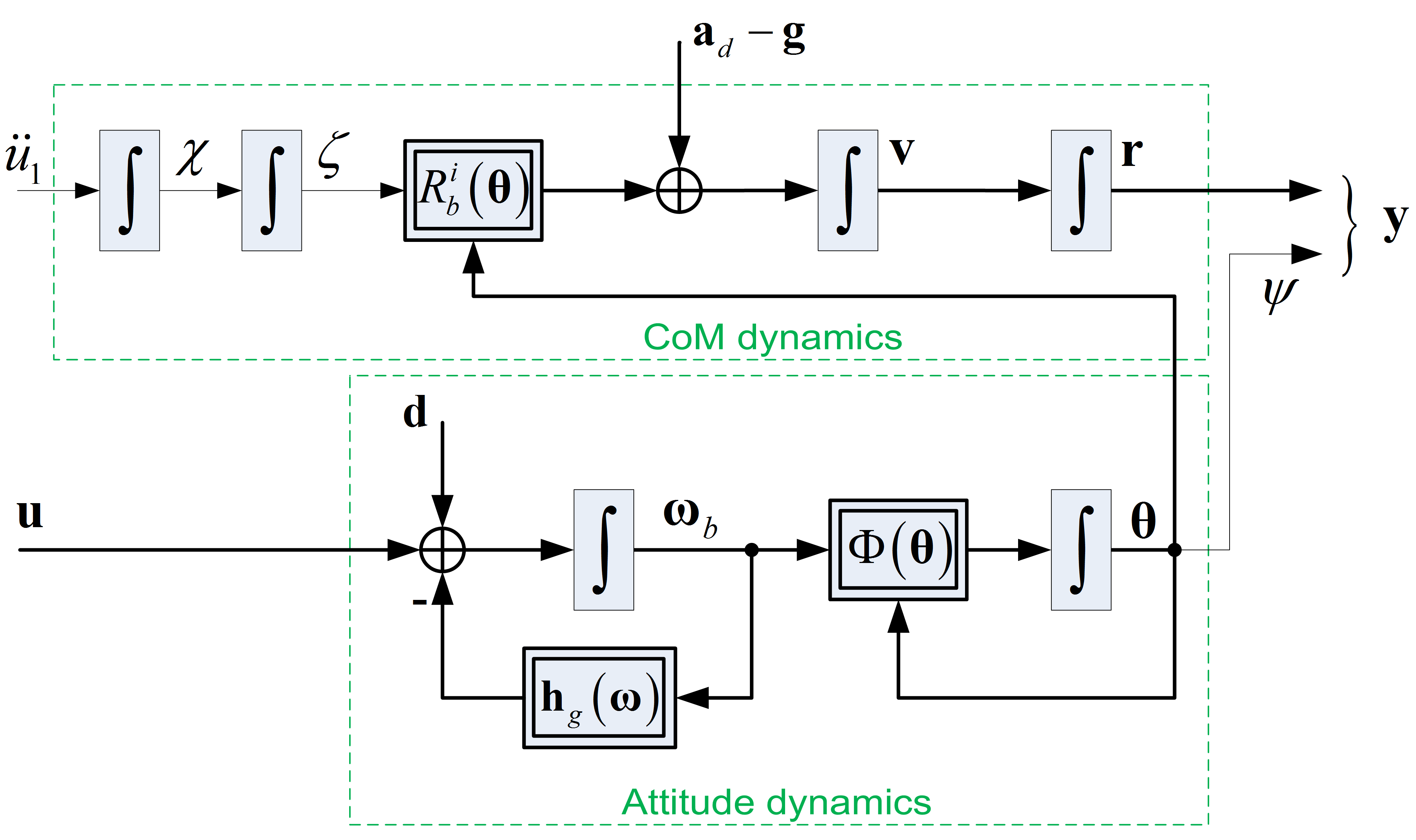
Figure 1: Quadrotor UAV extended Model.

The extended model (6) is the foremost building block of the feedback linearization process, performed to obtain the feedback-linearized model leveraged in [1] to design the internal model for the EMC state and disturbance predictor. To this aim, starting from the overall model in (6), we will derive the feedback-linearized heading and CoM dynamics, through the procedure outlined in Sec. II.

III-A The Quadrotor UAV Dynamics

Considering the quadrotor attitude kinematics in (6), let us start from the heading dynamics. The first order time-derivative of the heading angle holds:

$$\begin{split}\psi^{(1)}(t)&=\eta(t)=\mathbf{b}_{\psi}(\boldsymbol{\theta}(t))\boldsymbol{\omega}_{b}(t),\\ \mathbf{b}_{\psi}(\boldsymbol{\theta}(t))&=[-t_{\theta}c_{\psi}\quad t_{\theta}s_{\psi}\quad 1].\end{split}$$ (7)

A further derivative is needed in order to relate the output with the command, viz.:

$$\begin{split}\psi^{(2)}(t)&=\mathbf{b}_{\psi}(\boldsymbol{\theta}(t))(\mathbf{u}(t)-\mathbf{h}_{g}(t)+\mathbf{d}(t))+\dot{\mathbf{b}}_{\psi}(\boldsymbol{\theta}(t))\boldsymbol{\omega}_{b}(t)=\\ &=\mathbf{b}_{\psi}(\boldsymbol{\theta}(t))\mathbf{u}(t)+h_{\psi}(\mathbf{x}(t))+d_{\psi}(t),\end{split}$$ (8)

where we defined $h_{\psi}$ and $d_{\psi}$ as:

$$\begin{split}h_{\psi}(\mathbf{x}(t))&=\dot{\mathbf{b}}_{\psi}(\boldsymbol{\theta}(t))\boldsymbol{\omega}_{b}(t)-\mathbf{b}_{\psi}(\boldsymbol{\theta}(t))\mathbf{h}_{g}(t),\\ d_{\psi}(t)&=\mathbf{b}_{\psi}(\boldsymbol{\theta}(t))\mathbf{d}(t).\end{split}$$ (9)

Concerning the CoM dynamics, to relate the output with the command (cf. Sec. II), two derivatives will be needed; starting from the CoM acceleration.

Specifically, the CoM position third derivative, i.e. the jerk $\mathbf{s}$, holds:

$$\mathbf{r}^{(3)}(t)=\mathbf{s}(t)=\\ =R_{b}^{i}(\boldsymbol{\theta}(t))\left(\begin{bmatrix}0\\ 0\\ \chi(t)\end{bmatrix}+S(\boldsymbol{\omega}_{b}(t))\begin{bmatrix}0\\ 0\\ \zeta(t)\end{bmatrix}\right)+\dot{\mathbf{a}}_{d}(t),$$ (10)

being $S(\boldsymbol{\omega}_{b})$:

$$\begin{split}S(\boldsymbol{\omega}_{b})=\begin{bmatrix}0&-\omega_{z}&\omega_{y}\\ \omega_{z}&0&-\omega_{x}\\ -\omega_{y}&\omega_{x}&0\end{bmatrix}\end{split}.$$ (11)

In (10), the first term on the right-hand side represents the contribution of the vertical jerk command, whereas the second term is the jerk component due to the quadrotor angular rates.

Moreover, a further derivative of (10) is necessary in order to have a full-rank decoupling matrix $E(\cdot)$. Hence, it holds:

$$\mathbf{r}^{(4)}(t)=R_{b}^{i}(\boldsymbol{\theta}(t))\begin{bmatrix}\dot{\omega}_{y}\zeta\\ -\dot{\omega}_{x}\zeta\\ \ddot{u}_{1}\end{bmatrix}(t)+\\ +2\chi(t)R_{b}^{i}(\boldsymbol{\theta}(t))\begin{bmatrix}\omega_{y}\\ -\omega_{x}\\ 0\end{bmatrix}(t)+\\ +\zeta(t)R_{b}^{i}(\boldsymbol{\theta}(t))\begin{bmatrix}\omega_{x}\omega_{z}\\ \omega_{y}\omega_{z}\\ -(\omega_{x}^{2}+\omega_{y}^{2})\end{bmatrix}(t)+\ddot{\mathbf{a}}_{d}(t).$$ (12)

As a result, by introducing the quadrotor attitude dynamics from (6) in (12), we obtain:

$$\begin{split}\mathbf{r}^{(4)}(t)&=R_{b}^{i}(\boldsymbol{\theta}(t))\begin{bmatrix}\zeta u_{3}\\ -\zeta u_{2}\\ \ddot{u}_{1}\end{bmatrix}(t)+\mathbf{h}_{r}(\mathbf{x}(t))+\mathbf{d}_{r}(\mathbf{x}(t),t),\end{split}$$ (13)

where $\mathbf{h}_{r}$ and $\mathbf{d}_{r}$ are the known and the unknown disturbance terms, respectively. Specifically, $\mathbf{h}_{r}(\mathbf{x}(t))$ was defined as:

$$\mathbf{h}_{r}(t)=\zeta(t)R_{b}^{i}(\boldsymbol{\theta}(t))\begin{bmatrix}\omega_{x}\omega_{z}-h_{gy}\\ \omega_{y}\omega_{z}+h_{gx}\\ -(\omega_{x}^{2}+\omega_{y}^{2})\end{bmatrix}(t)+\\ +2\chi(t)R_{b}^{i}(\boldsymbol{\theta}(t))\begin{bmatrix}\omega_{y}\\ -\omega_{x}\\ 0\end{bmatrix}(t),$$ (14)

whereas $\mathbf{d}_{r}(\mathbf{x}(t))$ holds:

$$\begin{split}\mathbf{d}_{r}(\mathbf{x}(t))=R_{b}^{i}(\boldsymbol{\theta}(t))\begin{bmatrix}\zeta d_{ry}\\ -\zeta d_{rx}\\ 0\end{bmatrix}(t)+\ddot{\mathbf{a}}_{d}(t).\end{split}$$ (15)

From (15), it is interesting to notice how only tilt disturbances ($d_{rx}$, $d_{ry}$) act on the CoM dynamics, and how they are amplified by the body vertical acceleration $\zeta\,{=}\,u_{1}$, which is close to the gravity value for non aggressive manoeuvres [5].

III-B The Quadrotor UAV Case-study: Complete Model

As a further step, putting together the heading dynamics (8) and the CoM dynamics (13), the whole input-output relation is found:

$$\begin{bmatrix}\mathbf{r}^{(4)}\\ \psi^{(2)}\end{bmatrix}(t)=E(\boldsymbol{\theta}(t),\zeta(t))\overline{\mathbf{u}}(t)+\begin{bmatrix}\mathbf{h}_{r}\\ h_{\psi}\end{bmatrix}(t)+\begin{bmatrix}\mathbf{d}_{r}\\ d_{\psi}\end{bmatrix}(t),$$ (16)

where

$$\begin{split}E(\boldsymbol{\theta}(t),\zeta(t))&=\left[\begin{array}[]{c;{2pt/2pt}c}B_{r}(\boldsymbol{\theta}(t),\zeta(t))&\begin{array}[]{c}0\\ 0\\ 0\end{array}\\ \hdashline[2pt/2pt]\begin{array}[]{ccc}0&-t_{\theta}c_{\psi}&\quad t_{\theta}s_{\psi}\end{array}&1\end{array}\right]\\ B_{r}(\boldsymbol{\theta}(t),\zeta(t))&=R_{b}^{i}(\boldsymbol{\theta}(t))\begin{bmatrix}0&0&\zeta(t)\\ 0&-\zeta(t)&0\\ 1&0&0\end{bmatrix}.\end{split}$$ (17)

As shown in (3), the state vector of the new equivalent model (16) is defined by $\mathbf{z}\,{=}\,T(\mathbf{x})\,{=}\,[\mathbf{r}\>\>\mathbf{v}\>\>\mathbf{a}\>\>\mathbf{s}\>\>\psi\>\>\eta]^{T}$. More interestingly, the total relative degree of the model in (16) is equal to the order of the extended model in (6), namely $r_{1}\,{+}\,r_{2}\,{+}\,r_{3}\,{+}\,r_{4}\,{=}\,n\,{=}\,14$: this implies that no internal dynamics exists, and a full input-output linearization has been achieved.

Furthermore, the decoupling matrix $E(\mathbf{x}(t))$ is non-singular in $D\,{=}\,\{\mathbf{x}(t)\subset R^{n}:\zeta(t)\neq 0,|\phi(t)|<\pi/2,|\theta(t)|<\pi/2\}$. This implies that aggressive manoeuvres may be performed, although with tilt angles lower than $\pi/2$ (acrobatic manoeuvres, such as 360-loops, were not in the scope of [1]). On the other side, since the actuators effect is lower-bounded by a minimum saturation thrust, the total vertical acceleration is always positive. For these practical reasons, the state trajectories was constrained to the domain $D$, where the invertibility of the decoupling matrix is guaranteed.

To conclude, Figure 2 sketches the final model (16) (cf. also [1]), where the non-linear couplings with the commands $u_{2}$ and $u_{3}$ in $\mathbf{b}_{\psi}$ were collected in $h_{\psi}^{*}(\mathbf{x}(t),u_{2}(t),u_{3}(t))\,{=}\,-t_{\theta}c_{\psi}u_{2}(t)\,{+}\,t_{\theta}s_{\psi}u_{3}(t)$. On the other hand, $\mathbf{h}_{r}$ and $h_{\psi}$ collect all the non-linearities, collocated at command level. Finally, consistently with the EMC design framework, the terms $\mathbf{d}_{r}$ and $d_{\psi}$ represent the non-explicitly modelled effects and the external disturbances.

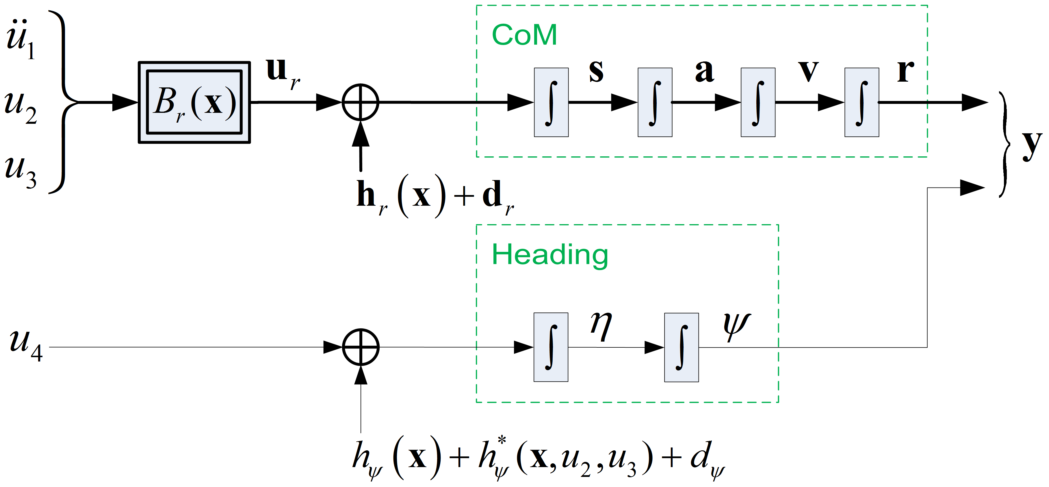
Figure 2: Global scheme of the quadrotor UAV input-output linearized model, as result of the FL technique (Courtesy: [1]).

As per Figure 2, for the purpose of the linear control design, the model (16) can be rewritten as:

$$\dot{\mathbf{r}}(t) =\mathbf{v}(t),\quad\mathbf{r}(0)=\mathbf{r}_{0},$$ (18a)

$$\dot{\mathbf{v}}(t) =\mathbf{a}(t),\quad\mathbf{v}(0)=\mathbf{v}_{0},$$ (18b)

$$\dot{\mathbf{a}}(t) =\mathbf{s}(t),\quad\mathbf{a}(0)=\mathbf{a}_{0},$$ (18c)

$$\dot{\mathbf{s}}(t) =\mathbf{u}_{r}(t)+\mathbf{h}_{r}(\mathbf{x}(t))+\mathbf{d}_{r}(t),\quad\mathbf{s}(0)=\mathbf{s}_{0},$$ (18d)

$$\dot{\psi}(t) =\eta(t),\quad\psi(0)=\psi_{0},$$ (18e)

$$\dot{\eta}(t) =u_{4}(t)+h_{\psi}(\mathbf{x}(t))+h_{\psi}^{*}(\cdot)+d_{\psi}(t),\quad\eta(0)=\eta_{0},$$ (18f)

where $\mathbf{u}_{r}$ is a transformed command, defined as:

$$\begin{split}\mathbf{u}_{r}(t)&=\mathbf{B}_{r}(\mathbf{x}(t))\begin{bmatrix}\ddot{u}_{1}&u_{2}&u_{3}\end{bmatrix}^{T}(t).\end{split}$$ (19)

As a result, 18a, 18b, 18c, 18d, 18e and 18f represent the UAV quadrotor model where all the non-linearities have been collocated at the command level and therefore can be cancelled by a non-linear feedback in the form expressed in (4). Nevertheless, this approach relies on the perfect knowledge of the model non-linearities ($\mathbf{h}_{r}$ , $h_{psi}$) which may considerably limit the controller performance as well as its practical applicability.

To this aim, the novel approach proposed in [1] (namely, the FL-EMC design) considers the model (18) from a different point of view. More precisely, the non-linear components are treated as generic unknown disturbances which are real-time estimated by a proper extended state observer. Thus, implementing a direct disturbance rejection, jointly with a linear control law, it is possible to completely neglect model non-linearities and, at same time, to enhance the controller robustness against model uncertainties.

References

- [1] M. A. Lotufo, L. Colangelo, and C. Novara, “Control design for uav quadrotors via embedded model control,” IEEE Transactions on Control Systems Technology, 2019.
- [2] H. K. Khalil, Noninear Systems. Prentice-Hall, New Jersey, 1996.
- [3] J.-J. E. Slotine, W. Li et al., Applied nonlinear control. Prentice hall Englewood Cliffs, NJ, 1991, vol. 199, no. 1.
- [4] V. Mistler, A. Benallegue, and N. K. M’Sirdi, “Exact linearization and noninteracting control of a 4 rotors helicopter via dynamic feedback,” in Proceedings 10th IEEE International Workshop on Robot and Human Interactive Communication. ROMAN 2001 (Cat. No.01TH8591), Sep. 2001, pp. 586–593.
- [5] M. A. Lotufo, L. Colangelo, C. Perez-Montenegro, C. Novara, and E. Canuto, “Embedded model control for uav quadrotor via feedback linearization,” IFAC-PapersOnLine, vol. 49, no. 17, pp. 266–271, 2016.