On the LoRa Modulation for IoT: Waveform Properties and Spectral Analysis

Abstract

An important modulation technique for Internet of Things (IoT) is the one proposed by the LoRa alliance™. In this paper we analyze the $M$-ary LoRa modulation in the time and frequency domains. First, we provide the signal description in the time domain, and show that LoRa is a memoryless continuous phase modulation. The cross-correlation between the transmitted waveforms is determined, proving that LoRa can be considered approximately an orthogonal modulation only for large $M$. Then, we investigate the spectral characteristics of the signal modulated by random data, obtaining a closed-form expression of the spectrum in terms of Fresnel functions. Quite surprisingly, we found that LoRa has both continuous and discrete spectra, with the discrete spectrum containing exactly a fraction $1/M$ of the total signal power.

I Introduction

The most typical IoT scenario involves devices with limited energy, that need to be connected to the Internet via wireless links. In this regard, Low Power Wide Area Networks aim to offer low data rate communication capabilities over ranges of several kilometers [1, 2, 3, 4]. Among the current communication systems, that proposed by the LoRa alliance (Low power long Range) [5] is one of the most promising, with an increasing number of IoT applications, including smart metering, smart grid, and data collection from wireless sensor networks for environmental monitoring [6, 7, 8, 9, 10, 11]. Several works discuss the suitability of the LoRa communication system when the number of IoT devices increases [12, 13, 14, 15].

The modulation used by LoRa, related to Chirp Spread Spectrum, has been originally defined by its instantaneous frequency [16]. Few recent papers attempted to provide a description of the low power long range (LoRa) modulation in the time domain, but, as will be detailed below, they are not complaint with the original LoRa signal model. The LoRa performance has been analyzed by simulation or by considering it as an orthogonal modulation [17, 18, 19]. On the other hand, the spectral characteristics of LoRa have not been addressed in the literature.

In this paper we provide a complete characterization of the LoRa modulated signal. In particular, we start by developing a mathematical model for the modulated signal in the time domain. The waveforms of this $M$-ary modulation technique are not orthogonal, and the loss in performance with respect to an orthogonal modulation is quantified by studying their cross-correlation. The characterization in the frequency domain is given in terms of the power spectrum, where both the continuous and discrete parts are derived. The found analytical expressions are compared with the spectrum of LoRa obtained by experimental data.

The main contributions of this paper can be summarized as follows:

• we provide the analytical expression of the signal for the $M$-ary LoRa chirp modulation in the time domain (both continuous-time and discrete-time);

• we derive the cross-correlation between the LoRa waveforms, and prove that the modulation is non-orthogonal;

• we prove that the waveforms are asymptotically orthogonal for increasingly large $M$;

• we derive explicit closed-form expressions of the continuous and discrete spectra of the LoRa signal in terms of the Fresnel functions;

• we prove that the power of the discrete spectrum is exactly a fraction $1/M$ of the overall signal power;

• we compare the analytical expression of the spectrum with experimental data from commercial LoRa devices;

• we show how the analytical expressions of the spectrum can be used to investigate the compliance of the LoRa modulation with the spectral masks regulating the out-of-band emissions and the power spectral density.

The provided time and spectral characterization of the LoRa signal is an analytical tool for the system design, as it allows suitable selection of the modulation parameters in order to fulfill the given requirements. For example, our analysis clarifies how the spreading factor, maximum frequency deviation, and transmitted power determine the occupied bandwidth, shape of the power spectrum and its compliance with spectrum regulations, system spectral efficiency, total discrete spectrum power, maximum cross-correlation, and SNR penalty with respect to orthogonal modulations.

Throughout the manuscript, we define the indicator function $g_{T}(t)=1$ for $0\leq t<T$ and $g_{T}(t)=0$ elsewhere, and indicate as $u(t)$ the unit step function. The Dirac’s delta is indicated as $\delta(x)$, and its discrete version as $\delta_{m}$, with $\delta_{0}=1$, $\delta_{m}=0\,\forall m\neq 0$. We also indicate with $C(x)\triangleq\int_{0}^{x}\cos\left(t^{2}{\pi}/{2}\right)\,dt$ and $S(x)\triangleq\int_{0}^{x}\sin\left(t^{2}{\pi}/{2}\right)\,dt\,$ the Fresnel functions[20].

II LoRa Signal Model

The LoRa frequency shift chirp spread spectrum modulation has been originally described in terms of the instantaneous frequency reported in [16, Figure 7]. It is an $M$-ary digital modulation, where the $M$ possible waveforms at the output of the modulator are chirp modulated signals over the frequency interval $(f_{0}-B/2,f_{0}+B/2)$ with $M$ different initial frequencies. The data modulated signal is usually preceded by synchronization waveforms, not considered here. For the data, the instantaneous frequency is linearly increased, and then wrapped to $f_{0}-B/2$ when it reaches the maximum frequency $f_{0}+B/2$, an operation that mathematically can be seen as a reduction modulo $B$. Having the instantaneous frequency sweeping over $B$ does not imply that the signal bandwidth is $B$, as will be discussed in Section III.

For LoRa the parameters are chosen such that $M=2^{\text{SF}}$ with SF integer, and $BT_{s}=M$, where $T_{s}$ is the symbol interval. The bit-rate of the modulation is

$$R_{b} =\frac{1}{T_{s}}\log_{2}M=\frac{\text{SF}}{T_{s}}=B\frac{\text{SF}}{2^{\text{SF}}}$$

The ratio between the chip-rate $R_{c}=M/T_{s}=B$ and the bit-rate is therefore

$$\eta=\frac{R_{c}}{R_{b}}=\frac{B}{R_{b}}=\frac{2^{\text{SF}}}{\text{SF}}\,.$$

Its reciprocal $1/\eta$ can be seen as the modulation spectral efficiency in bit/s/Hz. Some values of the spectral efficiency are reported in Table I for $M$ ranging from $2^{3}$ to $2^{12}$.

II-A Continuous-time description

To describe mathematically the signal in the time domain, let us start for clarity by assuming that the frequency interval over which to linearly sweep the frequency is $[0,B]$ as depicted in Fig. 1.

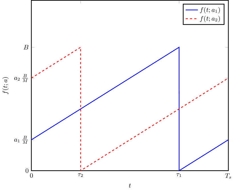
Figure 1: Example of the instantaneous frequency $f(t;a)$ as a function of time for two different modulating symbols $a_{1},a_{2}\in\{0,\ldots,M-1\}$.

For the time interval $t\in[0,T_{s}[$ and a symbol $a\in\{0,1,\ldots,M-1\}$ the instantaneous frequency in LoRa can thus be written as

$$f(t;a) =a\,\frac{B}{M}+\frac{B}{T_{s}}\,t\pmod{B}$$

$$=a\,\frac{B}{M}+\frac{B}{T_{s}}\,t-B\,u\left(t-\tau_{a}\right) 0\leq t<T_{s}$$ (1)

where $a\,{B}/{M}$ is the initial frequency which depends on the modulating symbol, and

$$\tau_{a}=T_{s}\left(1-\frac{a}{M}\right)$$ (2)

is the time instant where, after a linear increase, the instantaneous frequency reaches the maximum; for the remaining part of the symbol interval the instantaneous frequency is still linearly increasing, but reduced modulo $B$ by subtracting $B$.

Assuming the modulation starts at $t=0$, from (II-A) the phase $\phi(t;a)$ for $t\in[0,T_{s}[$ is given by

$$\phi(t;a) \triangleq 2\pi\int_{0}^{t}f(\tau,a)\,d\tau$$

$$=2\,\pi\left[a\,\frac{B}{M}\,t+\frac{B}{2\,T_{s}}\,t^{2}-B\,\left(t-\tau_{a}\right)\,u(t-\tau_{a})\right]\,.$$ (3)

Also, with the LoRa parameters we see from (2) that the product $B\tau_{a}=M-a$ is an integer, and can therefore be omitted in the phase.

Note that a factor $1/2$ for the quadratic term is missing in the phase definitions reported in [17, 18, 19], making the instantaneous frequency of the signal not complaint with that of LoRa. That difference also propagated in the discrete-time version of the signals used in [18, 19], so that even the time-discrete analysis made there is not applicable to the LoRa signal.

Property 1.

The LoRa modulation is a memoryless continuous phase modulation with $\phi(0;a)=\phi(T_{s};a)$.

Proof.

The initial phase is $\phi(0;a)=0$. The phase at the end of the symbol interval is

$$\phi(T_{s};a) =2\,\pi\left[a\,\frac{B}{M}T_{s}+\frac{B}{2}T_{s}-B\left(T_{s}-\tau_{a}\right)\,u(T_{s}-\tau_{a})\right]$$

$$=2\,\pi\left(a+\frac{M}{2}-M\,u(T_{s}-\tau_{a})\right)=0\pmod{2\pi}$$

where the last equality is due to that $a+{M}/{2}-Mu(T_{s}-\tau_{a})$ is always an integer. In other words, the initial and final phases are coincident, irrespectively on the symbol $a$. ∎

From this property we see that the LoRa modulation can be interpreted as a continuous phase memoryless modulation, where the transmitted waveform in each symbol interval depends only on the symbol in that interval, and not on previous or successive symbols. This can be visualized through the phase diagram which tracks the evolution of the phase over time. In Fig. 2, the phase diagram for two consecutive LoRa modulated symbols is shown as a function of time. It can be noted that each waveform starts and ends with the same phase.

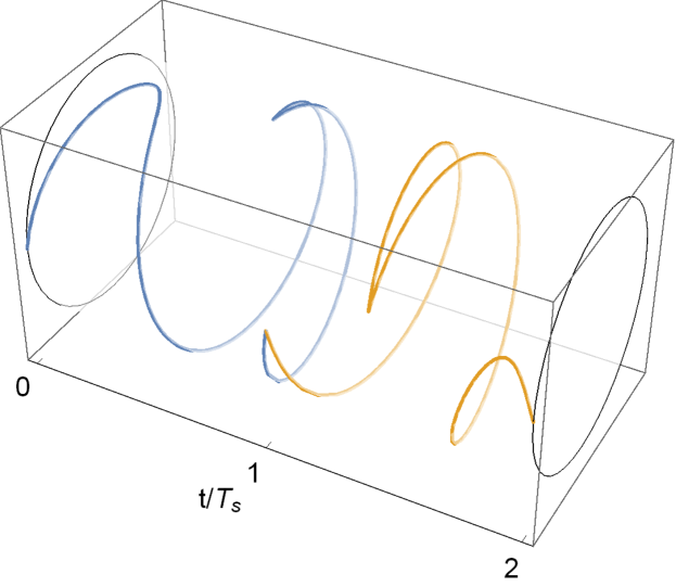
Figure 2: The phase diagram as a function of time over two consecutive LoRa modulated symbols, indicated in blue and orange.

The complex envelope of the modulated signal is

$$x(t;a) =\gamma\exp\left\{j\,\phi(t;a)\right\}, 0\leq t<T_{s}$$ (4)

where $\gamma=\sqrt{2\,P_{\text{s}}}$ accounts for the passband signal power $P_{\text{s}}$. In the following we will assume $\gamma=1$ unless otherwise stated. By introducing a frequency shift $-B/2$, the complex envelope centered at frequency zero for the interval $[0,T_{s}[$ is

$$\!\!\!\!x(t;a) =\exp\left\{j2\pi Bt\left[\frac{a}{M}\!-\!\frac{1}{2}\!+\!\frac{Bt}{2M}\!-\!u\left(t-\frac{M-a}{B}\right)\right]\right\}\,.$$ (5)

Due to the memoryless nature of the modulation, the complex envelope of the LoRa signal can be written as

$$i(t) =\sum_{n}x(t-nT_{s};a_{n})g_{T_{s}}(t-nT_{s})$$ (6)

where $a_{n}$ is the symbol transmitted in the time interval $[nT_{s},(n+1)T_{s}[$. We remark that, as this is a frequency modulated signal, we have $|i(t)|=1$ and the power of the signal $i(t)$ is one. The passband modulated signal centered at $f_{0}$ is then $s(t)=\Re\left\{i(t)e^{j2\pi f_{0}t}\right\}$.

TABLE I: Spectral efficiency, maximum cross-correlation, $99\%$-power bandwidth, total discrete spectrum power, and maximum SNR penalty.

$M=2^{\text{SF}}$	$1/\eta$	$\underset{\ell\neq m}{\max}\big{|}\Re\left\{C_{\ell,m}\right\}\big{|}$	$B_{99}$	$P_{\textrm{d}}$	$\Delta_{\max}$
	[bps/Hz]				[dB]
$2^{3}$	$0.375$	$0.212$	$1.500\,B$	$12.5\%$	$1.04$
$2^{5}$	$0.156$	$0.091$	$1.185\,B$	$3.125\%$	$0.41$
$2^{7}$	$0.055$	$0.045$	$1.045\,B$	$0.781\%$	$0.20$
$2^{10}$	$0.0098$	$0.015$	$0.990\,B$	$0.098\%$	$0.07$
$2^{12}$	$0.00293$	$0.0075$	$0.986\,B$	$0.024\%$	$0.03$

Property 2.

The cross-correlation between the continuous time waveforms $x(t;\ell)$ and $x(t;m)$ with $\ell\neq m$ is

$$C_{\ell,m} =\frac{1}{T_{s}}\int_{0}^{T_{s}}x(t;\ell)x^{*}(t;m)dt=$$

$$=M\frac{e^{j2\pi\ell(m-\ell)/M}-e^{j2\pi m(m-\ell)/M}}{j2\pi(M-|m-\ell|)|m-\ell|}$$ (7)

and $C_{\ell,\ell}=1$. It follows that the waveforms $x(t;\ell)$ and $x(t;m)$ are orthogonal (i.e, $C_{\ell,m}=0$) only for $|m-\ell|=2^{(p+\text{SF})/2}$ with $p\geq 0$ an odd (even) integer for odd (even) SF.

Moreover, since

$$\Re\left\{C_{\ell,m}\right\} =M\frac{\sin\left(\frac{2\pi\ell(m-\ell)}{M}\right)-\sin\left(\frac{2\pi m(m-\ell)}{M}\right)}{2\pi(M-|m-\ell|)|m-\ell|}$$ (8)

we have that the passband waveforms $\Re\left\{x(t;\ell)e^{j2\pi f_{0}t}\right\}$ and $\Re\left\{x(t;m)e^{j2\pi f_{0}t}\right\}$ are orthogonal (i.e, $\Re\left\{C_{\ell,m}\right\}=0$) only when $(m-\ell)^{2}/M$ is an integer, or when $(m^{2}-\ell^{2})/M-1/2$ is an integer.

Also, the maximum cross-correlation can be upper bounded as

$$\max_{\ell\neq m}\left|\Re\left\{C_{\ell,m}\right\}\right|\leq\max_{\ell\neq m}\left|C_{\ell,m}\right|\leq\frac{1}{\sqrt{2\,M}-1}.$$ (9)

Hence, the waveforms are asymptotically orthogonal for increasing $M$:

$$\lim_{M\to\infty}\left|\left\{C_{\ell,m}\right\}\right|=\delta_{\ell-m}\,.$$ (10)

Proof.

The crosscorrelation between the continuous time waveforms $x(t;\ell)$ and $x(t;m)$ with $\ell\neq m$ and $\ell>m$ can be written as

$$C_{\ell,m} =\frac{1}{T_{s}}\int_{0}^{T_{s}}e^{j2\pi\frac{B}{M}(\ell-m)\,t-B\,t\,\left[u\left(t-\tau_{\ell}\right)-u\left(t-\tau_{m}\right)\right]}\,dt$$

$$=\underbrace{\frac{1}{T_{s}}\int_{0}^{T_{s}}e^{j2\pi\frac{B}{M}(\ell-m)t}\,dt}_{0}-{\frac{1}{T_{s}}\int_{\tau_{\ell}}^{\tau_{m}}e^{j2\pi\frac{B}{M}(\ell-m)t}\,dt}$$

$$\phantom{=}+{\frac{1}{T_{s}}\int_{\tau_{\ell}}^{\tau_{m}}e^{j2\pi\left[\frac{B}{M}(\ell-m)\,t-B\,t\right]}\,dt}$$

$$=\frac{1}{j2\pi(\ell-m)}\left[e^{j2\pi(M-\ell)(\ell-m)/M}-e^{j2\pi(M-m)(\ell-m)/M}\right]$$

$$\phantom{=}+\!\frac{1}{j2\pi(M\!+m\!-\ell)}\left[\!e^{j2\pi\frac{(\ell-M)(M+m-\ell)}{M}}\!-e^{j2\pi\frac{(m-M)(M+m-\ell)}{M}}\!\right]$$

Noting the periodicity of the complex exponential function, we have

$$C_{\ell,m} =\frac{1}{j2\pi(\ell-m)}\left[e^{j2\pi\ell(m-\ell)/M}-e^{j2\pi m(m-\ell)/M}\right]$$

$$\phantom{=}+\frac{1}{j2\pi(M+m-\ell)}\left[e^{j2\pi\ell(m-\ell)/M}-e^{j2\pi m(m-\ell)/M}\right]$$

$$=\frac{e^{j2\pi\ell\frac{m-\ell}{M}}-e^{j2\pi m\frac{m-\ell}{M}}}{j2\pi}\left(\frac{1}{M+m-\ell}+\frac{1}{\ell-m}\right).$$ (11)

Similarly, for $m>\ell$ we have

$$C_{\ell,m} =\frac{e^{j2\pi\ell\frac{m-\ell}{M}}-e^{j2\pi m\frac{m-\ell}{M}}}{j2\pi}\left(\frac{1}{M+\ell-m}+\frac{1}{m-\ell}\right).$$ (12)

Putting together (11) and (12), the complex crosscorrelation, $C_{\ell,m}$, can be derived as in (2). The correlation in (2) can be zero only if the two exponentials are equal, that requires $\ell(m-\ell)/M=m(m-\ell)/M-k$, with $k$ an integer. Thus, it must be $|m-\ell|=\sqrt{kM}$. Since this must be an integer, and $M=2^{\text{SF}}$, it follows that $k=2^{p}$ with $p\geq 0$ an odd (even) integer for odd (even) SF.

The real cross-correlation (8) follows directly, and the conditions for its zeros are straightforward observing that $\sin\alpha=\sin\beta$ for $\alpha=\beta+k2\pi$ or $\alpha=\pi-\beta+k2\pi$.

In order to find the asymptotic behavior of the complex cross-correlation, we start by upper bounding its absolute value for $\ell\neq m$. From (2) we have

$$C_{\ell,m}=Me^{j2\pi\left(m^{2}-\ell^{2}\right)/M}\,\frac{e^{-j\pi(m-\ell)^{2}/M}-e^{j\pi(m-\ell)^{2}/M}}{j2\pi(M-|m-\ell|)|m-\ell|}$$

and therefore

$$\left|C_{\ell,m}\right|=M\frac{\left|\sin\left(\pi(m-\ell)^{2}/M\right)\right|}{\pi(M-|m-\ell|)|m-\ell|}\,.$$

The first maximum for $\left|C_{\ell,m}\right|$ is in the interval ${1\leq|m-\ell|\leq\left\lfloor{\sqrt{M/2}}\right\rfloor}$. This is due to the following reasons:

• $\left|C_{\ell,m}\right|$ is symmetric around $M/2$;

• the denominator is monotonically increasing for ${1\leq|m-\ell|\leq M/2}$;

• the numerator is monotonically increasing for $1\leq|m-\ell|\leq\left\lfloor{\sqrt{M/2}}\right\rfloor$, and starts to decrease after $\left\lfloor{\sqrt{M/2}}\right\rfloor$.

Hence, we have

$$\max_{\ell\neq m}\left|C_{\ell,m}\right| =\max_{1\leq|m-\ell|\leq\left\lfloor{\sqrt{M/2}}\right\rfloor}M\frac{\sin\left(\pi(m-\ell)^{2}/M\right)}{\pi(M-|m-\ell|)|m-\ell|}$$

$$\leq\max_{1\leq|m-\ell|\leq\left\lfloor{\sqrt{M/2}}\right\rfloor}\frac{|m-\ell|}{M-|m-\ell|}$$

$$\leq\frac{1}{\sqrt{2\,M}-1}$$

where for the first inequality $\sin(x)\leq x$ for $0\leq x\leq\pi/2$ is used. For the second inequality, it is noticed that the function is increasing in $|m-\ell|$, so its maximum value is obtained with $|m-\ell|=\left\lfloor{\sqrt{M/2}}\right\rfloor\leq\sqrt{M/2}$. Finally, taking the limit when $M\rightarrow\infty$ gives (10). ∎

The correlation among the waveforms of the LoRa modulation has an impact on the error performance for the optimum coherent receiver over AWGN channels [21, 22]. In particular, for the pairwise error probability between the $\ell$-th and $m$-th waveforms there is a factor $1-\Re\left\{C_{\ell,m}\right\}$ in the SNR with respect to orthogonal modulation schemes (see, e.g., equations (4.31) and (4.49) in [21]). In Table I we report the maximum penalty on the SNR, $\Delta_{\max}$, corresponding to the maximum cross-correlation, to be paid with respect to orthogonal modulation schemes. For example, with $M=2^{7}$ we have $\max_{\ell\neq m}\left|\Re\left\{C_{\ell,m}\right\}\right|=0.045$ and the maximum penalty is $\Delta_{\max}=0.2$ dB.

II-B Discrete-time description

For a simple receiver implementation it has been proposed to sample the received signal at chip rate, i.e., every $T_{c}=T_{s}/M=1/B$ seconds [16]. In this case we have in the interval $[0,T_{s}[$ the samples

$$x(kT_{c};a) =\exp\left\{j2\pi B\frac{kT_{s}}{M}\left[\frac{a}{M}-\frac{1}{2}+\frac{BkT_{s}}{2M^{2}}\right.\right.$$

$$\left.\left.\hskip 113.81102pt-u\left(k\frac{T_{s}}{M}-\frac{M-a}{B}\right)\right]\right\}$$

$$=\exp\left\{j2\pi k\left[\frac{a}{M}-\frac{1}{2}+\frac{k}{2\,M}-u\left(k\frac{T_{s}}{M}-\frac{M-a}{B}\right)\right]\right\}$$

$$=\exp\left\{j2\pi k\left(\frac{a}{M}-\frac{1}{2}+\frac{k}{2\,M}\right)\right\},\,k=0,1,\ldots,M-1$$ (13)

where the last equality is due to the fact that $2\pi k\,u(\cdot)$ is always an integer multiple of $2\pi$. This observation allows to avoid the modulus operation in the discrete-time description. Then, from (13) we have immediately the following property about the orthogonality of the discrete-time waveforms.

Property 3.

The discrete-time signals $x(kT_{c};a)$ are orthogonal in the sense that

$$\frac{1}{M}\sum_{k=0}^{M-1}x(kT_{c};\ell)x^{*}(kT_{c};m)=\delta_{\ell-m}$$ (14)

Proof.

From (13) we have

$$\frac{1}{M}\sum_{k=0}^{M-1}x(kT_{c};\ell)x^{*}(kT_{c};m) =\frac{1}{M}\sum_{k=0}^{M-1}e^{j2\pi k\left(\frac{\ell-m}{M}\right)}$$

$$=\delta_{\ell-m}$$

∎

As observed in [16, 18], once we have $x(kT_{c};a)$ we can compute the twisted (dechirped) vector $\tilde{\bf x}$ with elements

$$\tilde{x}_{k}=\tilde{x}(kT_{c};a) =x(kT_{c};a)e^{-j2\pi\frac{k^{2}}{2\,M}+j\pi k}\,.$$ (15)

Now, substituting (13) in (15), we see that

$$\tilde{x}_{k}=e^{j2\pi k\frac{a}{M}},\qquad k\in\{0,1,\ldots,M-1\}$$ (16)

which can be interpreted as a discrete-time complex sinusoid at frequency $a$. It follows that its Discrete Fourier Transform gives the vector ${\bf X}=\text{DFT}(\tilde{\bf x})$ with elements

$$X_{q} =\sum_{k=0}^{M-1}\tilde{x}(kT_{c};a)e^{-j2\pi kq/M}=\sum_{k=0}^{M-1}e^{-j2\pi k(q-a)/M}$$

$$=M\delta_{q-a},\qquad q\in\{0,1,\ldots,M-1\}\,.$$ (17)

Therefore, the DFT of the twisted signal (15) has only one non-zero element in the position of the modulating symbol $a$. This means that a possible way to implement a demodulator is to compute the dechirped vector (15), and decide based on its DFT.

Remark 1.

One could think now that working in the discrete-time domain we can achieve the performance of orthogonal modulations. However, this is not exactly the case, since, as will be shown in the next section, the bandwidth of the signal in (6) is larger than $B$. Therefore, filtering over a bandwidth $B$ will distort the signal, and the resulting samples will not be like in (13). As a consequence, they will not obey the orthogonality condition in (14). To avoid distortion, in general a bandwidth larger than $B$ should be kept before sampling. In the presence of AWGN, this will produce an increase in the noise power and correlation between noise samples with respect to an orthogonal modulation. However, for large $M$ the bandwidth of the signal stays approximately into a bandwidth $B$ (see next section and Table I), and therefore it is possible to implement a receiver based on sampling at rate $B$, dechirping, and looking for the maximum of the DFT. This is consistent with the observation that for large $M$ the modulation is approximately orthogonal (see Property 2).

III Spectral Analysis of the LoRa modulation

In this section, the power spectrum of the LoRa modulation is analytically derived in closed form in terms of Fresnel functions, or through the discrete Fourier transform. Then, it is shown that the modulated signal has a discrete spectrum containing a fraction $1/M$ of the overall signal power.

III-A Power Spectrum of LoRa Modulated Signals

Let us consider a source that emits a sequence of independent, identically distributed discrete random variables ${{A}}_{n}$ with probability

$$\mathbb{P}\{{{A}}_{n}=\ell\}=\frac{1}{M}, \forall\ell\in\{0,1,\cdots,M-1\}.$$

From (6) the modulator output can be represented by the stochastic process

$$I(t)=\sum_{n}x(t-nT_{s};{{A}}_{n})g_{T_{s}}(t-nT_{s})$$ (18)

where the random signal $x(t;\cdot)$ can take values in the set $\{x(t;\ell)\}_{\ell=0}^{M-1}$ of finite energy deterministic waveforms. The power spectral density of the random process $I(t)$ can be written as the sum of a continuous and a discrete parts

$$G_{I}(f)=G_{I}^{\textrm{c}}(f)+G_{I}^{\textrm{d}}(f)\,.$$ (19)

The expressions of the continuous and discrete spectra in (19) can be found by using for the random process (18) the frequency domain analysis of randomly modulated signals (see e.g. [21, 22]), obtaining

$$G_{I}^{\textrm{c}}(f) =\frac{1}{T_{s}\,M}\left[\sum_{\ell=0}^{M-1}\left|X(f;\ell)\right|^{2}-\frac{1}{M}\left|\sum_{\ell=0}^{M-1}X(f;\ell)\right|^{2}\right]$$ (20)

$$G_{I}^{\textrm{d}}(f) =\frac{1}{T_{s}^{2}\,M^{2}}\sum_{n=-\infty}^{\infty}\left|\sum_{\ell=0}^{M-1}X\left(n\frac{B}{M};\ell\right)\right|^{2}\,\delta\left(f-n\frac{B}{M}\right)$$ (21)

where $\{X(f;\ell)\}_{\ell=0}^{M-1}$ are the Fourier transforms of the waveforms $\{x(t;\ell)\}_{\ell=0}^{M-1}$ given in (5).

The spectrum can be derived analytically by expressing the Fourier transforms $X(f;\ell)$ in terms of Fresnel functions. More precisely, we have

$$\!\!\!X(f;\ell) \!\!=\!\!\int_{0}^{T_{s}}\!\!\!x(t;\ell)e^{-j2\pi ft}\,dt\!=\!\!\!\int_{0}^{\tau_{\ell}}\!\!\!e^{j2\pi\left[Bt(\frac{\ell}{M}\!-\!\frac{1}{2})+\!\frac{B^{2}}{2M}t^{2}\right]}e^{-j2\pi ft}dt$$

$$+\int_{\tau_{\ell}}^{T_{s}}e^{j2\pi\left[Bt(\frac{\ell}{M}-\frac{3}{2})+\frac{B^{2}}{2\,M}\,t^{2}\right]}\,e^{-j2\pi ft}\,dt.$$ (22)

Let us define the function

$$W(a;b;t_{1};t_{2}) =\int_{t_{1}}^{t_{2}}\exp\left({j2\pi\left[a\,t+b\,t^{2}\right]}\right)\,dt$$ (23)

that can be expressed in terms of the Fresnel functions as

$$W(a;b;t_{1};t_{2}) =\frac{1}{2\sqrt{b}}\,e^{-j2\pi\frac{a^{2}}{4\,b}}\left[K\left(2\sqrt{b}\,\left(t_{2}+\frac{a}{2\,b}\right)\right)-\right.$$

$$\left.K\left(2\sqrt{b}\,\,\left(t_{1}+\frac{a}{2\,b}\right)\right)\right]$$ (24)

where $K(x)\triangleq C(x)+j\,S(x)$. Then, the Fourier transform of the waveforms can be written analytically as

$$X(f;\ell) =W\left(B\left(\frac{\ell}{M}-\frac{1}{2}\right)-f;\frac{B^{2}}{2\,M};0;\frac{M-\ell}{B}\right)+$$

$$W\left(B\left(\frac{\ell}{M}-\frac{3}{2}\right)-f;\frac{B^{2}}{2\,M};\frac{M-\ell}{B};\frac{M}{B}\right)\,$$ (25)

that used in (20) and (21) gives the signal spectrum.

An alternative to the use of the Fresnel functions consists in the standard Discrete Fourier Transform approach, where we take $N$ samples of $x(t;\ell)$ over the time interval $[0,T_{s}[$ in a vector ${\bf{x}}(\ell)=\{x(0;\ell),x(\Delta_{t};\ell),\cdots,x((N-1)\Delta_{t};\ell)\}$, with step $\Delta_{t}=T_{s}/N$. Then, the vector ${\bf{X}}(\ell)=\Delta_{t}\,\text{DFT}({\bf{x}}(\ell))$ gives the samples with frequency step $\Delta_{f}=1/T_{s}=B/M$ of the periodic repetition $\sum_{k}X(f-kF;\ell)$, where $F=N/T_{s}=NB/M$. For sufficiently large $N$ the effect of aliasing is negligible, so that the elements of ${\bf{X}}(\ell)$ are essentially the samples of $X(f;\ell)$ with step $\Delta_{f}$. For the discrete spectrum this frequency step is exactly what is needed in (21). If a finer resolution in frequency is needed (for the continuous spectrum in (20)) we have to zero-pad the vector ${\bf{x}}(\ell)$ before taking the DFT. For example, if we add $(k-1)N$ zeros to ${\bf{x}}(\ell)$ the frequency step is $\Delta_{f}=1/kT_{s}=B/kM$.

III-B Total Power of the Discrete spectrum

Lines in the spectrum indicates the presence of a non-zero mean value of the signal, which does not carry information. The following property quantifies the power of this mean value with respect to the overall signal power.

Property 4.

The total power of the discrete spectrum for the LoRa modulation

$$P_{\textrm{d}} =\int_{-\infty}^{\infty}G_{I}^{\textrm{d}}(f)\,df=\frac{1}{T_{s}^{2}\,M^{2}}\sum_{n=-\infty}^{\infty}\left|\sum_{\ell=0}^{M-1}X\left(n\frac{B}{M};\ell\right)\right|^{2}\,$$

is exactly a fraction $1/M$ of the overall signal power.

Proof.

The discrete spectrum in (21) is due to the mean value of the signal

$${\mathbb{E}}\left\{{I(t)}\right\}=\sum_{n}{\mathbb{E}}\left\{{x(t-nT_{s};{{A}}_{n})}\right\}g_{T_{s}}(t-nT_{s})\,.$$

This mean value is not zero, implying that there are lines in the spectrum[22, 21]. More precisely, since the modulation is memoryless, we have for $0\leq t<T_{s}$

$${\mathbb{E}}\left\{{x(t;A_{0})}\right\}=\frac{1}{M}\sum_{\ell=0}^{M-1}x(t;\ell)=\frac{1}{M}\sum_{\ell=0}^{M-1}\sum_{k=0}^{M-1}x(t;\ell)$$

$$\phantom{=}\times g_{T_{c}}\left(t-k\,T_{c}\right)=\frac{1}{M}\sum_{k=0}^{M-1}g_{T_{c}}\left(t-k\,T_{c}\right)\sum_{\ell=0}^{M-1}x(t;\ell)$$

$$=\frac{1}{M}\left\{g_{T_{c}}(t)\sum_{\ell=0}^{M-1}x(t;\ell)+\sum_{k=1}^{M-1}g_{T_{c}}\left(t-k\,T_{c}\right)\sum_{\ell=0}^{M-1}x(t;\ell)\right\}$$

where $T_{c}=1/B$ is the chip rate. From (5) we have

$${\mathbb{E}}\left\{{x(t;A_{0})}\right\}=\frac{1}{M}e^{j2\pi\frac{B}{2T_{s}}\,t^{2}}\left\{g_{T_{c}}(t)\sum_{\ell=0}^{M-1}e^{j2\pi\frac{B}{M}\ell\,t}\right.+$$

$$\left.\sum_{k=1}^{M-1}g_{T_{c}}\left(t-k\,T_{c}\right)\left[\sum_{\ell=0}^{M-k-1}e^{j2\pi\frac{B}{M}\ell\,t}+\sum_{\ell=M-k}^{M-1}e^{j2\pi\frac{B}{M}\ell\,t}e^{-j2\pi Bt}\right]\right\}$$

$$=\frac{1}{M}e^{j2\pi\frac{B}{2T_{s}}\,t^{2}}\left\{g_{T_{c}}(t)\frac{1-e^{j2\pi Bt}}{1-e^{j2\pi Bt/M}}+\sum_{k=1}^{M-1}g_{T_{c}}\left(t-k\,T_{c}\right)\right.$$

$$\phantom{=}\left.\times e^{j2\pi B(M-k)t/M}\frac{e^{-j2\pi Bt}-1}{1-e^{j2\pi Bt/M}}\right\}.$$

After some manipulation we get

$${\mathbb{E}}\left\{{x(t;A_{0})}\right\} =\frac{1}{M}e^{j\frac{\pi Bt}{M}(Bt-1)}\frac{\sin\left(\pi Bt\right)}{\sin\left(\pi Bt/M\right)}$$

$$\phantom{=}\times\sum_{k=0}^{M-1}g_{T_{c}}\left(t-k\,T_{c}\right)\,e^{-j2\pi Bkt/M}.$$

The absolute value of the mean is therefore

$$|{\mathbb{E}}\left\{{x(t;A_{0})}\right\}| =\frac{1}{M}\left|\frac{\sin\left(\pi Bt\right)}{\sin\left(\pi Bt/M\right)}\right|, 0\leq t<T_{s}\,.$$

Now, recalling the following integral for $m$ integer [23, p. 396]

$$\int_{0}^{\pi/2}\left(\frac{\sin mx}{\sin x}\right)^{2}dx=\frac{\pi}{2}$$

we get the power of the discrete spectrum as

$$P_{\textrm{d}}=\frac{1}{T_{s}}\int_{0}^{T_{s}}|{\mathbb{E}}\left\{{x(t;A_{0})}\right\}|^{2}\,dt=\frac{1}{M}\,.$$ (26)

Therefore, there are lines in the spectrum of the LoRa modulation, and the power of this discrete spectrum is a fraction $1/M$ of the overall power. ∎

IV Numerical Results

We first show in Fig. 3 the two-sided power spectrum of the complex envelope for LoRa modulated signals as a function on the normalized frequency $f/B$, with various spreading factors, i.e., $\text{SF}\in\{3,7,10,12\}$. Since $G_{I}(-f)=G_{I}(f)$ we just show $G_{I}(f)$ for $f\geq 0$.

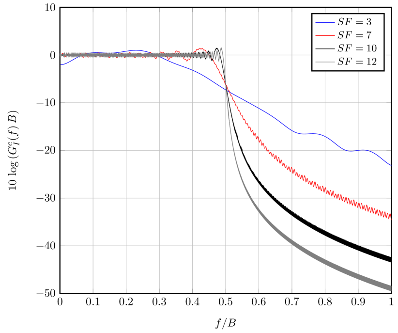
(a) The continuous part of the spectrum

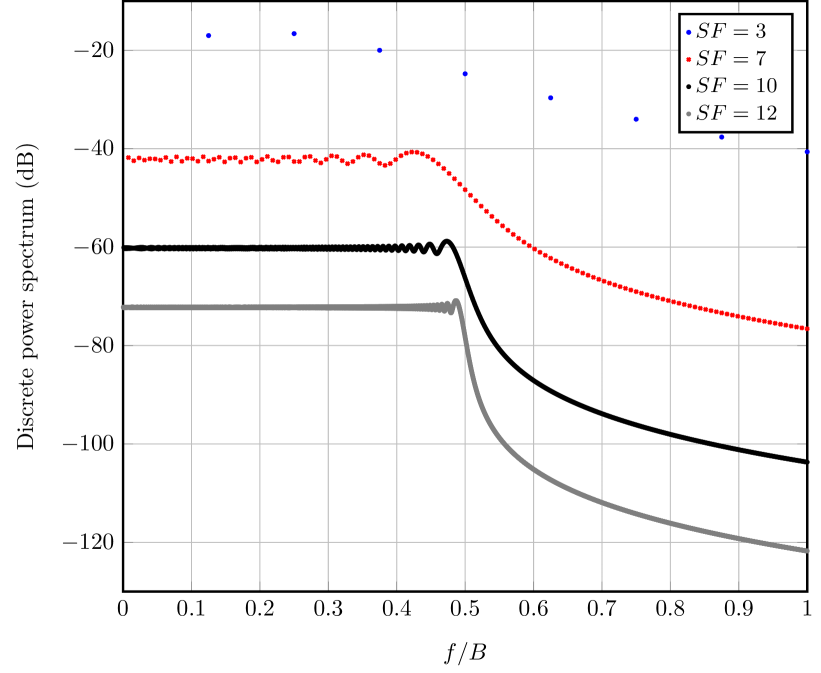
(b) The discrete spectrum

Figure 3: The continuous and discrete spectrum of the complex envelope for LoRa modulation, $M=2^{\text{SF}}$, with $\text{SF}\in\{3,7,10,12\}$.

In the figure we report both the normalized power spectral density, $10\,\log_{10}G^{c}_{I}(f)\,B$, and the discrete part of the spectrum. For the latter we report the power $\left|\sum_{\ell=0}^{M-1}X\left(n{B}/{M};\ell\right)\right|^{2}/{T_{s}^{2}\,M^{2}}$ at frequency $nB/M$, as given in (21). The sum of the power of all lines in the discrete spectrum is equal to $1/M$, as proved in Property 4. For example, with $\text{SF}=3$ we have $M=8$ and thus $1/M=12.5\%$ of the signal power is contained in the discrete spectrum. We can see that the power spectrum becomes more compact for increasing $M$, so that most of the power for the complex envelope is contained between $-B/2$ and $B/2$, or, in other words, that the modulated signal bandwidth is close to $B$ for large $M$.

To better quantify this effect, we report in Table I the bandwidth $B_{99}$ centered on $f_{0}$ containing $99\%$ of the power for different spreading factors. It can be seen that, while for $M\geq 2^{7}$ almost all of the signal is contained in a bandwidth $B$, considering just a bandwidth $B$ for smaller spreading factors will leave out a part of the signal, therefore distorting the signal. Moreover, as noted in Section II and Section III, the spectral efficiency, the maximum real cross-correlation, and the power of the discrete spectrum decrease for increasing $M$.

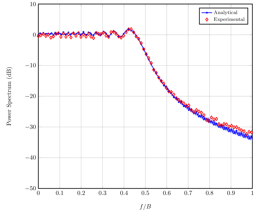
(a) $\text{SF}=7$

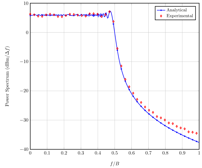
(b) $\text{SF}=10$

Figure 4: The power spectrum of the complex envelope for LoRa modulation using the analytical expressions and the experimental data, for $M=2^{\text{SF}}$, $\text{SF}\in\{7,10\}$, $B=125$ kHz, $\Delta f=B/256$, and $P_{\text{s}}=27$ dBm.

In Fig. 4, we compare the derived analytical power spectrum with that obtained from the IQ samples of a commercially available LoRa transceiver [24]. More precisely, IQ samples are provided for LoRa modulated waveforms, which have been created with a randomly generated payload of $16$ bytes. The waveforms are obtained for $B=125~{}$kHz with sample rate $f_{s}=4\,B$ [24]. The frequency range of interest is divided into several bins with width $\Delta f=B/256$, and the power within each bin is computed either analytically via (20) and (21), or through spectral estimation by implementing the Welch’s method on the experimental data[25]. It is noticed that the estimated spectrum agrees well with the analytical expression. We can also observe that the tail of the estimated spectrum is slightly higher than the analytical; this is because the experimental samples have been taken at $f_{s}=4\,B$, not large enough to completely eliminate frequency aliasing.

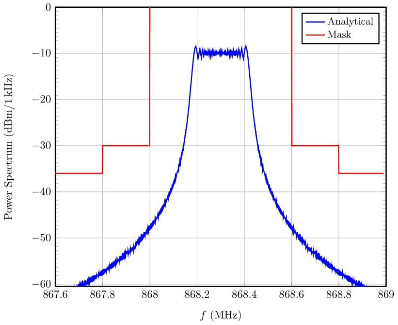
(a) One channel, $B=250$ kHz.

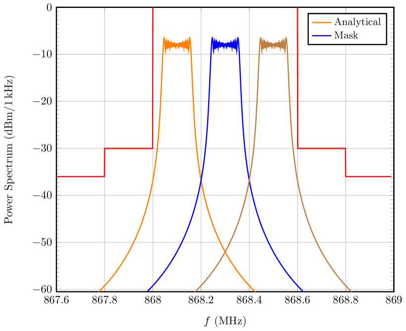
(b) Three channels, $B=125$ kHz.

Figure 5: The one-sided power spectrum for LoRa modulated passband signals using the analytical expressions, compared with the mask from the ETSI regulation in the G1 sub-band, for $M=2^{7}$, $\Delta f=1$ kHz, and $P_{\text{s}}=14$ dBm.
a) One channel with center frequency $868.3$ MHz for $B=250$ kHz. b) Three channels with center frequencies $868.1$ MHz, $868.3$ MHz, and $868.5$ MHz for $B=125$ kHz.

Finally, we investigate the LoRa spectrum along with the ETSI regulations for out-of-band emissions [26, 7.7.1]. Since LoRa is a chirp spread spectrum technique, it is governed by the regulations for ISM bands that support wideband modulation [26, Table 5]. For example, we consider the G1 sub-band spanning from $868$ MHz to $868.6$ MHz[26, Fig. 7]. There are two possibilities for using LoRa in this sub-band:

• using a single channel with center frequency $868.3$ MHz for $B=250$ kHz;

• using three channels with center frequencies $868.1$, $868.3$, and $868.5$ MHz for $B=125$ kHz.

In Fig. 5 we report, for the two cases above, the one-sided power spectrum calculated analytically with bin width (i.e., resolution bandwidth) $\Delta f=1$ kHz, and $P_{\text{s}}=14$ dBm, i.e., the maximum allowed transmission power. The spectrum is compared with the spectral mask for the G1 sub-band. It can be noticed that the spectrum meets the regulations of the maximum power limits for adjacent band emissions at the G1 sub-band. The same method can be used to examine the LoRa compliance for various ISM bands, spreading factors, and bandwidths, according to other regional regulations.

V Conclusions

In this paper we investigated the spectral characteristics of the LoRa $M$-ary modulation, deriving the analytical expression of the spectrum, and comparing it with experimental data and with the spectral limit masks for the ISM bands. We found that there are lines in the spectrum, containing a fraction $1/M$ of the overall power, and that the occupied bandwidth is in general larger than the deviation $B$. We also derived the waveform cross-correlation function, proving that the LoRa waveforms can be considered orthogonal only for asymptotically large $M$.

References

- [1] M. Centenaro, L. Vangelista, A. Zanella, and M. Zorzi, “Long-range communications in unlicensed bands: the rising stars in the IoT and smart city scenarios,” IEEE Wireless Commun., vol. 23, no. 5, pp. 60–67, Oct. 2016.
- [2] U. Raza, P. Kulkarni, and M. Sooriyabandara, “Low power wide area networks: An overview,” IEEE Commun. Surveys Tuts., vol. 19, no. 2, pp. 855–873, Jan. 2017.
- [3] F. Adelantado, X. Vilajosana, P. Tuset-Peiro, B. Martinez, J. Melia-Segui, and T. Watteyne, “Understanding the limits of LoRaWAN,” IEEE Commun. Mag., vol. 55, no. 9, pp. 34–40, Sept. 2017.
- [4] E. Morin, M. Maman, R. Guizzetti, and A. Duda, “Comparison of the device lifetime in wireless networks for the Internet of things,” IEEE Access, vol. 5, pp. 7097–7114, 2017.
- [5] “A technical overview of LoRa and LoRaWAN,” LoRa Alliance Technical Marketing Workgroup, Tech. Rep., 2015.
- [6] H. Sherazi, G. Piro, L. Grieco, and G. Boggia, “When renewable energy meets LoRa: A feasibility analysis on cable-less deployments,” IEEE Internet Things J., pp. 1–12, May 2018.
- [7] W. Zhao, S. Lin, J. Han, R. Xu, and L. Hou, “Design and implementation of smart irrigation system based on LoRa,” in IEEE Globecom Workshop, Singapore, Singapore, Dec 2017, pp. 1–6.
- [8] H. Lee and K. Ke, “Monitoring of large-area IoT sensors using a LoRa wireless mesh network system: Design and evaluation,” IEEE Trans. Instrum. Meas., vol. 67, no. 9, pp. 2177–2187, Sept 2018.
- [9] L. Feltrin, C. Buratti, E. Vinciarelli, R. D. Bonis, and R. Verdone, “LoRaWAN: Evaluation of link- and system-level performance,” IEEE Internet Things J., vol. 5, no. 3, pp. 2249–2258, June 2018.
- [10] G. Pasolini, C. Buratti, L. Feltrin, F. Zabini, C. De Castro, R. Verdone, and O. Andrisano, “Smart city pilot projects using LoRa and IEEE802.15.4 technologies,” Sensors, vol. 18, no. 4, p. 1118, 2018.
- [11] M. Alahi, N. Pereira-Ishak, S. Mukhopadhyay, and L. Burkitt, “An Internet-of-Things enabled smart sensing system for Nitrate monitoring,” IEEE Internet Things J., pp. 1–1, 2018.
- [12] O. Georgiou and U. Raza, “Low power wide area network analysis: Can LoRa scale?” IEEE Wireless Commun. Lett., vol. 6, no. 2, pp. 162–165, April 2017.
- [13] F. V. den Abeele, J. Haxhibeqiri, I. Moerman, and J. Hoebeke, “Scalability analysis of large-scale LoRaWAN networks in Ns-3,” IEEE Internet Things J., vol. 4, no. 6, pp. 2186–2198, Dec 2017.
- [14] J. Lim and Y. Han, “Spreading factor allocation for massive connectivity in LoRa systems,” IEEE Commun. Lett., vol. 22, no. 4, pp. 800–803, April 2018.
- [15] D. Croce, M. Gucciardo, S. Mangione, G. Santaromita, and I. Tinnirello, “Impact of LoRa imperfect orthogonality: Analysis of link-level performance,” IEEE Commun. Lett., vol. 22, no. 4, pp. 796–799, April 2018.
- [16] F. Sforza, “Communications system,” 2013, US Patent 8,406,275.
- [17] B. Reynders and S. Pollin, “Chirp spread spectrum as a modulation technique for long range communication,” in Proc. Symposium on Communications and Vehicular Technologies (SCVT), Mons, Belgium, Nov 2016, pp. 1–5.
- [18] L. Vangelista, “Frequency shift chirp modulation: The LoRa modulation,” IEEE Signal Process. Lett., vol. 24, no. 12, pp. 1818–1821, Dec 2017.
- [19] T. Elshabrawy and J. Robert, “Closed form approximation of LoRa modulation BER performance,” IEEE Commun. Lett., pp. 1–5, June 2018.
- [20] M. Abramowitz and I. A. Stegun, Handbook of Mathematical Functions wih Formulas, Graphs, and Mathematical Tables. New York, NY, United States: Dover Publications, 1974, vol. 55.
- [21] S. Benedetto and E. Biglieri, Principles of digital transmission: with wireless applications. Berlin/Heidelberg, Germany: Springer Science & Business Media, 1999.
- [22] J. G. Proakis, Digital communications. New York City, United States: McGraw-Hill, 1995.
- [23] I. S. Gradshteyn and I. M. Ryzhik, Tables of Integrals, Series, and Products, 7th ed. San Diego, CA: Academic Press, Inc., 2007.
- [24] Semtech LoRa, “LoRa IQ waveform library,” 2018. [Online]. Available: https://semtech.force.com/lora
- [25] P. Welch, “The use of fast Fourier transform for the estimation of power spectra: A method based on time averaging over short, modified periodograms,” IEEE Trans. Audio Electroacoust., vol. 15, no. 2, pp. 70–73, June 1967.
- [26] “ETSI EN 300 220-1 V2.4.1,” European Telecommunications Standards Institute, Tech. Rep., 2012.