Applying the tempered Lefschetz thimble method to the Hubbard model away from half-filling
Abstract
The tempered Lefschetz thimble method is a parallel-tempering algorithm towards solving the numerical sign problem. It uses the flow time of the gradient flow as a tempering parameter and is expected to tame both the sign and multimodal problems simultaneously. In this paper, we further develop the algorithm so that the expectation values can be estimated precisely with a criterion ensuring global equilibrium and the sufficiency of the sample size. To demonstrate that this algorithm works well, we apply it to the quantum Monte Carlo simulation of the Hubbard model away from half-filling on a two-dimensional lattice of small size, and show that the numerical results agree nicely with exact values.
I Introduction
The sign problem is one of the major obstacles when performing numerical calculations in various fields of physics. Typical examples include finite density QCD [1], quantum Monte Carlo (QMC) calculations of quantum statistical systems [2, 3, 4], and the numerical simulations of real-time quantum field theories.
Among a variety of approaches, two algorithms have taken attention as potential candidates to generically solve the sign problem for systems with complex action; one is the complex Langevin method [5], and the other is a class of algorithms utilizing the Lefschetz thimbles [6, 7, 8, 9, 10, 11, 12, 13, 14, 15]. Although both the algorithms make use of complexification of variables and analytic continuation of integrands, their methodologies are fairly different; the former algorithm attempts to replace the complex Boltzmann weight by a real positive weight defined in the whole complex space, while the latter deforms the integration region in the complex space so as to reduce the phase oscillation. At this stage, each algorithm has its own advantage and disadvantage. The former is advantageous in that it is relatively fast with computational cost (: the degrees of freedom), but it suffers from the so-called wrong convergence problem [16, 17, 18, 19]. The latter is generally free from the wrong convergence problem if only a single thimble is relevant in evaluating the expectation values of physical observables of interest. The disadvantage is its expensive numerical cost, which is because of the need to calculate the Jacobian determinant. When multiple thimbles are relevant, one needs to take care of the multimodality of the distribution. The tempered Lefschetz thimble method (TLTM) was thus proposed in [14] to tame both the sign and multimodal problems simultaneously, where the system is tempered by the flow time of the antiholomorphic gradient flow (see also [15] for a similar idea).
In this paper, we further develop the TLTM, proposing an algorithm which allows the precise estimation of expectation values with a criterion ensuring global equilibrium and the sufficiency of the sample size. The key is the use of the fact that the expectation values should be the same for all flow times. To demonstrate that this algorithm works well, we apply it to the QMC simulation of the Hubbard model away from half-filling.
The application of Lefschetz thimble methods to the Hubbard model has already been considered by several groups [20, 21, 22] (see also [23, 24] for recent study), and the relevance of the contributions from multiple thimbles has been reported. In this paper, we consider a two-dimensional periodic square lattice of size with the inverse temperature decomposed to pieces, and numerically evaluate the expectation values of observables as functions of the chemical potential with other parameters fixed to some values. We show that the TLTM (the implementation of tempering combined with the above algorithm for precise estimation) give results that agree nicely with exact values, simultaneously resolving the sign and multimodal problems.
We comment that the extent of seriousness of the sign problem in the QMC simulation of the Hubbard model depends heavily on the choice of the Hubbard-Stratonovich variables. In this paper, in order to apply the Lefschetz thimble method, we exclusively consider a Gaussian Hubbard-Stratonovich variable that leads to a complex action. There the sign problem is actually severe as we will see below, and one needs to seriously consider a dilemma between the sign and multimodal problems, which can be solved by the TLTM as stated above. However, the temporal size considered here is still small (), and for such a high temperature regime one can resort to other methods than the Lefschetz thimble methods with a different type of Hubbard-Stratonovich variables (see discussions in section III).
This paper is organized as follows. In section II after briefly reviewing the TLTM [14], we give a new algorithm which allows the precise estimation of expectation values with a criterion ensuring global equilibrium and the sufficiency of the sample size. This algorithm is applied to the Hubbard model in section III, and we discuss about the obtained numerical results. We there also make a comment on the sign averages obtained by other methods. Section IV is devoted to conclusion and outlook. Five appendices are given for more detailed discussions on various topics.
II Tempered Lefschetz thimble method
Let be a real -dimensional dynamical variable with action which may take complex values. Our main concern is to estimate the expectation values
| (1) |
We assume that and are entire functions over when is complexified to . Then, due to Cauchy’s theorem for higher dimensions, the right-hand side does not change under continuous deformations of the integration region as long as the boundary at infinity is kept fixed so that the integrals converge. The sign problem will get reduced if is almost constant on the new integration region.
In [11, 11, 12, 13, 14, 15] such a deformation () is made according to the antiholomorphic gradient flow:
| (2) |
Equation (1) can then be rewritten as
| (3) |
which can be further rewritten as a ratio of reweighted integrals over by using the Jacobian matrix [11]:
| (4) |
Here, and are defined by
| (5) | ||||
| (6) |
and obeys the following differential equation [11] (see also footnote 2 of [14]):
| (7) |
with . Under the flow (2), the action changes as , and thus increases except at the critical points (), while is kept constant. In particular, in the limit , the deformed region will approach a union of -dimensional submanifolds (Lefschetz thimbles) on each of which is constant, and thus the sign problem is expected to disappear there (except for a possible residual sign problem arising from the phase of the complex measure and a possible global sign problem caused by phase cancellations among different thimbles). However, in the Monte Carlo calculation one cannot take the limit naïvely, because the potential barriers between different thimbles become infinitely high so that the whole configuration space cannot be explored sufficiently. This multimodality of distribution makes the Monte Carlo calculation impractical, especially when contributions from more than one thimble are relevant to estimating expectation values. A key proposal in [12] is to use a finite value of flow time that is large enough to avoid the sign problem but simultaneously is not too large so that the exploration in the configuration space is still possible. However, it is a difficult task to find such value of flow time in a systematic way, as we will discuss at the end of section III and in Appendix E.
The TLTM [14] is a tempering algorithm that uses the flow time as a tempering parameter. There, the global relaxation of the multimodal distribution is prompted by enabling configurations around different modes to easily communicate through transitions in ensembles at smaller flow times. Among other possible tempering algorithms, the parallel tempering algorithm [25, 26] (also known as the replica exchange MCMC method; see [27] for a review) is adopted in the TLTM [14] because it does not need to introduce the probability weight factors of ensembles at various flow times and because most of relevant steps can be done in parallel processes.
In the TLTM (see Appendix A for the summary of the algorithm), we first fix the maximum flow time which should be sufficiently large such that the sign problem is reduced there. A possible criterion is that the sign average is in the absence of tempering. This process can be carried out by a test run with small statistics. We then enlarge the configuration space from to the set of replicas, . We assign to replicas () the flow times with . The action at replica , , is obtained by solving (2) and (7) with its own initial conditions , . We set up an irreducible, aperiodic Markov chain for the enlarged configuration space such that the probability distribution for eventually approaches the equilibrium distribution proportional to
| (8) |
This can be realized by combining (a) the Metropolis algorithm (or the Hybrid Monte Carlo algorithm) in the direction at each fixed flow time and (b) the swap of configurations at two adjacent replicas. Each of the steps (a) and (b) can be done in parallel processes. After the system is well relaxed to global equilibrium, we estimate the expectation value at flow time [see (4)] by using the subsample at replica , , that is retrieved from the total sample :
| (9) |
The original proposal in [14] is to use (9) at the maximum flow time, , as an estimate of .
Recall here that the left-hand side of (9) is independent of due to Cauchy’s theorem, and thus the ratio should yield the same value within the statistical error margin if the system is well in global equilibrium. In practice, this is not true for small ’s due to the sign problem, where the estimate of the sign average, , can be smaller than its statistical error (; the value for the uniform distribution of phases). In this case, the statistical error of the ratio cannot be trusted, which means that such should not be used as an estimate of .
Based on the observation above, we now propose an algorithm which allows a precise estimation of with a criterion ensuring global equilibrium and the sufficiency of the sample size. First, we continue the sampling until we find some range of (to be denoted by ) in which are well above and take the same value within the statistical error margin. We will require that the intervals around be above . Then, we estimate by using the fit for with a constant function of . Global equilibrium and the sufficiency of the sample size are checked by looking at the optimized value of . Note that the parameters determined by this procedure (such as , , ) can vary depending on the choice of observable .
We close this section with a few comments. First, in the TLTM a sufficient overlap of the distributions at adjacent replicas is expected even for large flow times as long as the spacings are not too large. This is because the distributions at large ’s () have peaks at the same points in that flow to critical points in . This is in sharp contrast with the situation in other tempered systems, where the distribution often changes rapidly as a function of the tempering parameter so that an enough overlap cannot be achieved for realistically meaningful small spacings. Second, the optimal form of is a linear function of when flowed configurations are close to a critical point. This is because the optimal choice for the overall coefficients in tempering algorithms is exponential (see, e.g., [28, 29]) and because the real part of the action grows exponentially in flow time near critical points. Finally, the computational cost in the TLTM is expected to be due to the increase caused by the tempering algorithm (which will be ). Note that this growth of computational cost can be compensated by increasing the number of parallel processes.
III Application to the Hubbard model away from half-filling
Let be a -dimensional lattice with lattice points. The Hubbard model describes nonrelativistic lattice fermions of spin one-half, and is defined by the Hamiltonian (including the chemical potential)
| (10) |
Here, and are the annihilation and creation operators on site with spin obeying the anticommutation relations and , and . is the adjacency matrix that takes a nonvanishing value () only for nearest neighbors, and we assume the lattice to be bipartite. is the hopping parameter, is the chemical potential, and represents the strength of the on-site repulsive potential. We have shifted as so that corresponds to the half-filling state, .
We approximate the grand partition function by using the Trotter decomposition with equal spacing (), and rewrite it as a path integral over a Gaussian Hubbard-Stratonovich variable . Then the expectation value of the number density is expressed as (see Appendix B for the derivation)
| (11) | ||||
| (12) | ||||
| (13) | ||||
| (14) |
where and is a product in descending order. Note that in (14) can be replaced by , which is more preferable in Monte Carlo calculations because statistical errors will be reduced due to the averaging over . The charge-charge correlation, (), can also be evaluated as a path integral by simply replacing by when . As for the observables that are not directly constructed from , the expectation values can be evaluated by using the formula (42).
We now apply the TLTM to the Hubbard model on a two-dimensional periodic square lattice of size (thus ) with . We first estimate numerically by using the expressions (11)–(14) for various values of with other parameters fixed to be , . Note that the physical quantities depend only on the dimensionless parameters , , for fixed .
The complex action (12) gives rise to a serious sign problem, as can be seen in the left panel of Fig. 1.


However, we should note that the extent of the seriousness of the sign problem heavily depends on the choice of the Hubbard-Stratonovich variables, and actually, the sign problem can be avoided for the above parameters within the BSS (Blankenbecler, Scalapino and Sugar)-QMC method [30]. In fact, the right panel of Fig. 1 shows the sign averages calculated by using a public code called ALF (Algorithms for Lattice Fermions) [31] that is based on the discrete variables introduced in [32, 33]. We see that the sign averages are above 0.98 for all the range of studied here.111 We thank a referee for suggesting us to investigate this point.
Following the general prescription and writing with , we introduce the enlarged configuration space . We here brief the setup of the parameters relevant to the TLTM (see Appendix D for more details). We set to be piecewise linear in with a single breakpoint whose position will be tuned such that the acceptance rates of the swapping process at adjacent replicas are almost the same for all pairs (being roughly above 40%).222 This functional form of is best suited to the case where the deformed region reaches the vicinity of all the relevant Lefschetz thimbles at almost the same flow time and such a linear form is effective also for the transient period. For each value of , we make a test run with small statistics to adjust parameters. This gives the values –, –, –, varying on the value of . We make a sampling after discarding 5,000 configurations, and from the obtained data we estimate by using the fit.
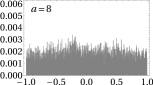
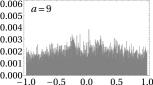
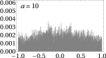
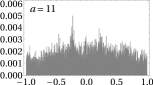
As an example, let us see Fig. 2, which shows and at various replicas for .
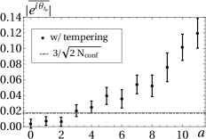
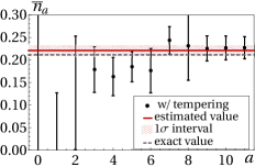
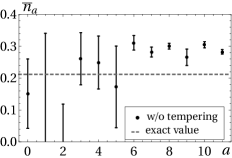
The left panel shows that the intervals around are above for (and thus we set and ). The right panel shows that the data in this range give the same value within the statistical error margin. The fit gives the estimate (exact value: 0.212) with .
Figure 3 shows the thus-obtained numerical estimates of as a function of .
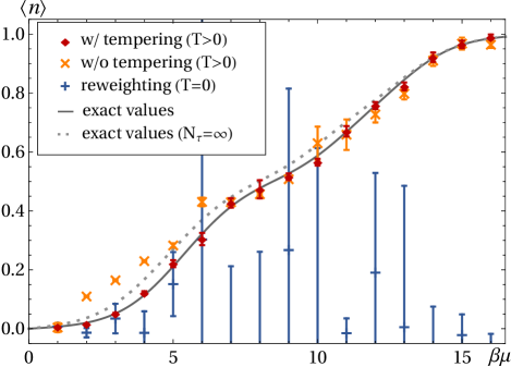
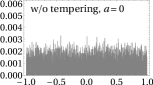
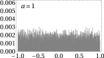
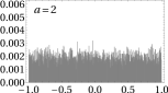
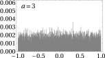
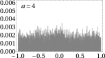
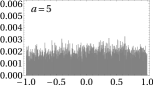
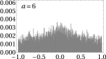
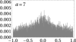
We also display the estimates obtained without tempering (at the same maximum flow times ) and those from the original reweighting method (i.e. ), together with the values obtained by the explicit evaluation of the trace under the Trotter decomposition with and for the continuum imaginary time (i.e. ) (see Appendix C). We see that the exact values are correctly reproduced when the tempering is implemented, while there are significant deviations when not implemented. As in the -dimensional massive Thirring model [14], the deviation reflects the fact that the relevant thimbles are not sampled sufficiently. In fact, from Fig. 4, which shows the distribution of averaged flowed configurations at for ,


we see that, although the flowed configurations are widely distributed over many thimbles when the tempering is implemented, they are restricted to only a small number of thimbles when not implemented.
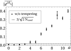
Three comments are in order. First, a larger value of the sign average does not necessarily mean a better resolution of the sign problem, as can be seen from Fig. 5. In fact, when only a very few thimbles are sampled, the sign average can become larger than the value in the correct sampling due to the absence of phase mixtures among different thimbles.
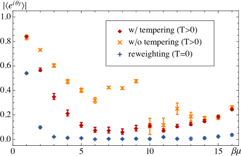
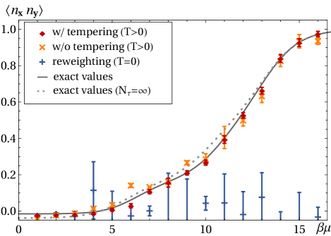
Second, whether the multimodality can affect the estimates of expectation values depends on the choice of observables. In fact, from the discrepancies of the sign averages in Fig. 5, we see that the multimodality must be severe in the region . However, the estimates of almost agree between the two methods with and without tempering in the range . This means that the operator is not sensitive to the multimodality in this range. To find an observable that is sensitive to the multimodality, we estimated the nearest-neighbor charge-charge correlation with the same sample.333We thank the referee for suggesting us to investigate the expectation values of observables other than the number density operator. The results are shown in Fig. 6, where we see a significant discrepancy at between the two methods.
Such discrepancies become more manifest if we look at the observables that are not directly constructed from the number density operator . As an example, we show in Fig. 7 the expectation values of the kinetic energy operator (without the factor “”) , which are estimated for the same sample as above by using the formula (42).
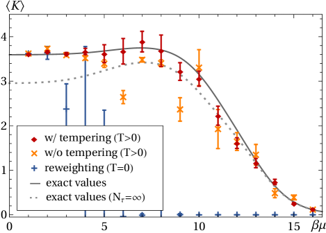
We there notice two things. One is that the discrepancies between the two methods now become significant for all the range . The other is that the precision of the TLTM becomes worse compared to the case for the observables that are constructed solely from . In fact, those observables that are not directly constructed from (such as ) contain matrix elements of , and may have divergently large values in the vicinity of zeros of the fermion determinants . In this case, precise estimation will require a larger sample size and a more accuracy in integrating flow equations compared with operators constructed solely from . We expect that a similar attention must be paid when one applies the TLTM to finite density QCD. We leave a further investigation of this point as a future investigation.
Finally, from Fig. 8, we see that it should be a difficult task to find an intermediate flow time (without tempering) that avoids both the sign problem (severe at smaller flow times) and the multimodal problem (severe at larger flow times) (see Appendix E for more detailed discussions).
Generically, flowed configurations repeatedly experience the event at which they get trapped to fewer number of Lefschetz thimbles, so that there is a large ambiguity in distinguishing the larger and smaller flow times in the first place.
IV Conclusion and outlook
In this paper, we proposed an algorithm for the TLTM which allows a precise estimation of expectation values. We confirm the effectiveness by applying it to the two-dimensional Hubbard model away from half-filling.
We should stress that our study in this paper is still at an exploratory level. In fact, the lattice must be enlarged much more both in the spatial and imaginary time directions to claim the validity of our method for the sign problem in the Hubbard model, revealing the phase structure of the model. In doing this, it should be important to check whether the computational scaling is actually as expected.
More generally, we should keep developing the algorithm further so that it can be more easily applied to the three major problems listed in Introduction. There should also be other interesting branches of fields where the TLTM may shed new light on the theoretical understanding through a numerical analysis, such as the Chern-Simons theory [34] and matrix models that generate random volumes [35].
When we were preparing the first version of the manuscript, there appeared an interesting paper [23] (see also its detailed version [24]), where the sign and ergodicity problems are also studied for the Lefschetz thimble method applied to the Hubbard model away from half-filling. In our method (TLTM), the two problems are solved simultaneously by tempering the system with the flow time, where one does not need to know a detailed structure of thimbles. In contrast, in [23, 24] they redundantly introduce two continuous Gaussian Hubbard-Stratonovich variables with a parameter representing the mixture of the two variables (see also [22]). With knowledge of thimble structures, they tune the parameter in such a way that only a few number of thimbles become relevant to the evaluation, and obtain results for a hexagonal lattice with and . It would be interesting to introduce such redundant integration variables also in the TLTM so as to reduce the global sign problem (possible cancellation of phases among different thimbles), which we observe also depends heavily on the choice of integration variables.
Acknowledgements.
The authors thank Yoshimasa Hidaka, Issaku Kanamori, Norio Kawakami, Yoshio Kikukawa, Jun Nishimura, Akira Ohnishi, Masaki Tezuka, Asato Tsuchiya and Urs Wenger for useful discussions. They also thank an anonymous referee of Physical Review D for giving us valuable comments, which were very helpful in improving the first version of the manuscript. This work was partially supported by JSPS KAKENHI (Grant Numbers 16K05321, 18J22698 and 17J08709) and by SPIRITS 2019 of Kyoto University (PI: M.F.).Appendix A Summary of the algorithm
We summarize the algorithm of the TLTM (we partially repeat the presentation of [14]):
Step 0. We fix the maximum flow time which should be sufficiently large such that the sign problem is reduced there. A possible criterion is that the sign average is in the absence of tempering. This can be carried out by a test run with small statistics. We then pick up flow times from the interval with . The values of and are determined manually or adaptively to optimize the acceptance rate in Step 3 below. Practically, once is determined, can be chosen to be a piecewise linear function of [see the argument for (74)].
Step 1. For each replica , we choose an initial value and numerically solve the differential equations (2) and (7) to obtain the triplet .
Step 2. For each replica , we use the Metropolis algorithm to update the value of . To be explicit, we take a value from using a symmetric proposal distribution, and recalculate the triplet using the as the initial value. We then update to with the probability , where
| (15) |
We repeat the process sufficiently many times such that local equilibrium is realized for each . Step 1 and Step 2 can be performed in parallel processes.
Step 3. We swap the configurations at two adjacent replicas and by updating to with the probability
| (16) |
One can easily see that this satisfies the detailed balance condition with respect to the global equilibrium distribution (8) because
| (17) |
We repeat the process several times so as to reduce autocorrelations. This procedure can also be performed in parallel processes by choosing a set of independent pairs.
Step 4. By repeating Step 2 and Step 3, we obtain a sequence of triplets,
| (18) |
for each , with which we estimate the expectation value at flow time :
| (19) |
Here, is chosen to be large enough so that we find some range of (to be denoted by with ) in which the intervals around are above and take the same value within the statistical error margin.
Step 5. The expectation value of is estimated by the fit from the data with a constant function of . Global equilibrium and the sufficiency of the sample size is checked by looking at the optimized value of .
In the above algorithm, we have implicitly assumed that the action at does not exhibit multimodality. If this is not the case, we further introduce other parameters (such as the overall coefficient of the action) as extra tempering parameters or prepare flow times with [14].
Appendix B Derivation of eqs. (11)–(14)
For a bipartite lattice, we specify which sublattice x belongs to by the sign . We first make the so-called particle-hole transformation, and . Then the one-body part and the two-body part of the Hamiltonian (10) are rewritten, respectively, as
| (20) | ||||
| (21) |
In the last equation, we have used the identity and . Note that the number density operator is written as
| (22) |
In order to perform a Monte Carlo simulation, we approximate in the grand partition function by using the Trotter decomposition with equal spacing ():
| (23) |
and rewrite at the -th position from the right to the exponential of a fermion bilinear by using a Gaussian Hubbard-Stratonovich variable :
| (24) |
Then, the approximated grand partition function takes the following path integral form:
| (25) |
Here, , and the action is given by
| (26) |
where is an ordered product (), and (or ) represents the trace over the Fock space created by (or by ). The fermion trace in (26) can be evaluated explicitly by using the following formulas that hold for the operator constructed from an matrix :
| (27) | |||
| (28) |
(The first equation can be readily proved by the fact that is a Lie algebra homomorphism. The second equation can be easily understood by moving to a diagonalizing basis for .) We thus find that the action becomes
| (29) | ||||
| (30) |
where is a diagonal matrix of the form . Note that, while the action is real-valued for the half-filling case due to the identity , it is generically complex-valued when .
The expectation values of such observables that are made solely from the number density operators can be evaluated as a path integral over by simply replacing by , as easily proved by using the operator identity
| (31) |
For example, the expectation value of the number density operator, , can be rewritten to a path integral form as in (11).
As for observables of general form, one can resort to the Wick-Bloch-de Dominicis theorem,
| (35) |
to obtain the following expression:
| (42) |
where .
Appendix C Evaluation of the trace under the Trotter decomposition
The Hilbert space of the Hubbard model after the particle-hole transformation is the tensor product of two Fock spaces, , each constructed by acting or on the Fock vacuum . In this appendix, we give the explicit forms of the matrix elements that appear in the trace under the Trotter decomposition:
| (43) |
Here, the one-body part and the two-body part of the Hamiltonian are given by [see (20) and (21)]
| (44) | ||||
| (45) | ||||
| (46) | ||||
| (47) |
The number density operator is given by
| (48) |
and we have introduced the transfer matrices corresponding to and :
| (49) |
We first introduce a one-dimensional ordering to the set of all spatial coordinates, , and take a basis of to be
| (50) |
where the states
| (51) | ||||
| (52) |
are labeled by the subsets of ordered coordinates, (with ), (with ). We will denote their sizes by , .
The matrix elements of are then given by the following determinants:
| (56) | |||
| (60) | |||
| (61) |
as can be easily proven by investigating the action of on the state :
| (62) |
where the coefficients do not vanish only when . The matrix elements of can also be given in the forms of determinant,
| (66) | |||
| (67) |
We thus obtain the explicit forms of the matrix elements .
As for , we note that acts on diagonally:
| (68) |
The coefficients can be calculated easily to be
| (69) |
where is the logical step function and stands for the complement of the set , . The matrix elements of is then given by .
Finally, the matrix elements of are given by
| (70) |
With the matrix elements given above, can be expressed as
| (71) |
Appendix D Summary of the parameters in the computation
We summarize the parameters relevant to the TLTM in the estimation of . We order the termination times for replicas as (: the largest flow time), and set to be a piecewise linear function of with a single breakpoint at , by assuming that the deformed region reaches the vicinity of all the relevant Lefschetz thimbles at almost the same flow time and that the linear form is effective also for the transient period:
| (74) |
Each Monte Carlo step consists of 50 Metropolis tests in the direction and swaps of configurations at adjacent replicas, and the flow equations (2) and (7) are integrated numerically by using the adaptive Runge-Kutta of 7-8th order. For each value of , we make a test run with small statistics and adjust the parameters , , in such a way that the acceptance rates of the swapping process at adjacent replicas are almost the same for all pairs (being roughly above 40%). After this, we make another test run of 1,000 data points to adjust the width of the Gaussian proposal in the Metropolis test in the direction so that the acceptance rate is in the range 50%–80%. This width varies depending on replicas and the values of . Using the adjusted parameters, we get a sample of size after discarding 5,000 configurations, and analyze the data by using the Jackknife method, with bins whose sizes are adjusted by taking account of autocorrelations. Finally, from the obtained data [see (9)], we estimate the expectation value by using the fit with a constant function of . We confirm that the system is in global equilibrium and the sample size is sufficient by looking at the optimized value of with . The obtained results are summarized in Table 1.
| 1 | 2 | 3 | 4 | 5 | 6 | 7 | 8 | |
| 1/10 | 1/10 | 1/10 | 1/10 | 1/10 | 1/11 | 1/11 | 1/12 | |
| 8 | 9 | 10 | 11 | 11 | 11 | 11 | 11 | |
| 0.7 | 0.6 | 0.6 | 0.6 | 0.6 | 0.5 | 0.5 | 0.5 | |
| 5 | 5 | 6 | 6 | 6 | 5 | 5 | 5 | |
| 10 | 10 | 12 | 12 | 12 | 12 | 12 | 12 | |
| 5k | 5k | 10k | 10k | 15k | 25k | 15k | 15k | |
| 0 | 0 | 2 | 3 | 5 | 5 | 6 | 7 | |
| 0.53 | 0.43 | 0.47 | 0.12 | 0.45 | 0.39 | 1.07 | 0.72 |
| 9 | 10 | 11 | 12 | 13 | 14 | 15 | 16 | |
| 1/12 | 1/12 | 1/12 | 1/11 | 1/11 | 1/11 | 1/11 | 1/11 | |
| 11 | 11 | 12 | 12 | 12 | 12 | 12 | 12 | |
| 0.5 | 0.55 | 0.55 | 0.6 | 0.6 | 0.6 | 0.6 | 0.6 | |
| 5 | 5 | 6 | 6 | 6 | 7 | 7 | 7 | |
| 12 | 12 | 14 | 14 | 14 | 14 | 14 | 14 | |
| 10k | 10k | 10k | 10k | 5k | 5k | 5k | 5k | |
| 8 | 8 | 10 | 8 | 9 | 10 | 9 | 9 | |
| 0.09 | 0.92 | 0.21 | 1.74 | 0.40 | 0.17 | 0.75 | 0.20 |
Appendix E More on the fine-tuning of flow time without tempering
In order to understand the difficulty to find such an intermediate value of flow time that avoids both the sign and multimodal problems (without tempering), let us see the right panel of Fig. 8, which is the counterpart of Fig. 2 (with tempering) for the same . We see that the estimated values have large statistical errors at smaller flow times (due to the sign problem) while they have small statistical errors around incorrect values at larger flow times (due to the trapping of configurations at a small number of thimbles). The best flow time must be at the boundary between the two regions, but it should be a difficult task to find such value out of the set of flow times with finite spacings. In fact, if one takes a flow time from the smaller region, then, although the obtained estimate may happen to be close to the correct value, it must have a large statistical error. On the other hand, if a flow time is taken from the larger region, it will give an incorrect value (but with a small statistical error because only a small number of thimbles are sampled).
In order to understand Fig. 2 and Fig. 8 as reflecting the extent of the sign and multimodal problems, let us see Fig. 9, which depicts the normalized histograms of phases for with tempering (top) and without tempering (bottom).
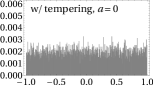
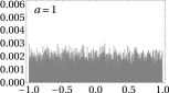
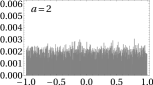
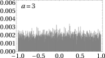
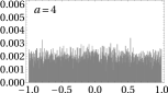
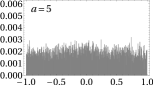
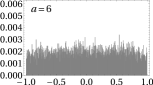
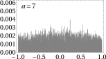
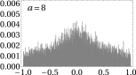
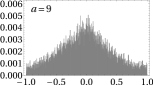
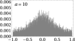
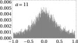
We see that at smaller flow times the histograms are almost flat for the both cases (giving rise to the sign problem), but at larger flow times those without tempering become almost unimodal (reflecting the trapping at a small number of thimbles) while those with tempering correctly come to have various peaks (which may not be so obvious from the figure because there are many peaks and each peak is broadened by the Jacobian determinant).
References
- [1] G. Aarts, “Introductory lectures on lattice QCD at nonzero baryon number,” J. Phys. Conf. Ser. 706, no. 2, 022004 (2016) [arXiv:1512.05145 [hep-lat]].
- [2] J. E. Hirsch, “Two-dimensional Hubbard model: Numerical simulation study,” Phys. Rev. B 31, 4403 (1985).
- [3] E. Y. Loh, J. E. Gubernatis, R. T. Scalettar, S. R. White, D. J. Scalapino and R. L. Sugar, “Sign problem in the numerical simulation of many-electron systems,” Phys. Rev. B 41, 9301 (1990).
- [4] L. Pollet, “Recent developments in Quantum Monte-Carlo simulations with applications for cold gases,” Rep. Prog. Phys. 75, 094501 (2012) [arXiv:1512.05145 [hep-lat]].
- [5] G. Parisi, “On Complex Probabilities,” Phys. Lett. 131B, 393 (1983).
- [6] M. Cristoforetti, F. Di Renzo and L. Scorzato, “New approach to the sign problem in quantum field theories: High density QCD on a Lefschetz thimble,” Phys. Rev. D 86, 074506 (2012) [arXiv:1205.3996 [hep-lat]].
- [7] M. Cristoforetti, F. Di Renzo, A. Mukherjee and L. Scorzato, “Monte Carlo simulations on the Lefschetz thimble: Taming the sign problem,” Phys. Rev. D 88, no. 5, 051501(R) (2013) [arXiv:1303.7204 [hep-lat]].
- [8] A. Mukherjee, M. Cristoforetti and L. Scorzato, “Metropolis Monte Carlo integration on the Lefschetz thimble: Application to a one-plaquette model,” Phys. Rev. D 88, no. 5, 051502(R) (2013) [arXiv:1308.0233 [physics.comp-ph]].
- [9] H. Fujii, D. Honda, M. Kato, Y. Kikukawa, S. Komatsu and T. Sano, “Hybrid Monte Carlo on Lefschetz thimbles - A study of the residual sign problem,” JHEP 1310, 147 (2013) [arXiv:1309.4371 [hep-lat]].
- [10] M. Cristoforetti, F. Di Renzo, G. Eruzzi, A. Mukherjee, C. Schmidt, L. Scorzato and C. Torrero, “An efficient method to compute the residual phase on a Lefschetz thimble,” Phys. Rev. D 89, no. 11, 114505 (2014) [arXiv:1403.5637 [hep-lat]].
- [11] A. Alexandru, G. Başar and P. Bedaque, “Monte Carlo algorithm for simulating fermions on Lefschetz thimbles,” Phys. Rev. D 93, no. 1, 014504 (2016) [arXiv:1510.03258 [hep-lat]].
- [12] A. Alexandru, G. Başar, P. F. Bedaque, G. W. Ridgway and N. C. Warrington, “Sign problem and Monte Carlo calculations beyond Lefschetz thimbles,” JHEP 1605, 053 (2016) [arXiv:1512.08764 [hep-lat]].
- [13] A. Alexandru, G. Başar, P. F. Bedaque, G. W. Ridgway and N. C. Warrington, “Monte Carlo calculations of the finite density Thirring model,” Phys. Rev. D 95, no. 1, 014502 (2017) [arXiv:1609.01730 [hep-lat]].
- [14] M. Fukuma and N. Umeda, “Parallel tempering algorithm for integration over Lefschetz thimbles,” PTEP 2017, no. 7, 073B01 (2017) [arXiv:1703.00861 [hep-lat]].
- [15] A. Alexandru, G. Başar, P. F. Bedaque and N. C. Warrington, “Tempered transitions between thimbles,” Phys. Rev. D 96, no. 3, 034513 (2017) [arXiv:1703.02414 [hep-lat]].
- [16] J. Ambjørn and S. K. Yang, “Numerical Problems in Applying the Langevin Equation to Complex Effective Actions,” Phys. Lett. 165B, 140 (1985).
- [17] G. Aarts, F. A. James, E. Seiler and I. O. Stamatescu, “Complex Langevin: Etiology and Diagnostics of its Main Problem,” Eur. Phys. J. C 71, 1756 (2011) [arXiv:1101.3270 [hep-lat]].
- [18] G. Aarts, L. Bongiovanni, E. Seiler, D. Sexty and I. O. Stamatescu, “Controlling complex Langevin dynamics at finite density,” Eur. Phys. J. A 49, 89 (2013) [arXiv:1303.6425 [hep-lat]].
- [19] K. Nagata, J. Nishimura and S. Shimasaki, “Argument for justification of the complex Langevin method and the condition for correct convergence,” Phys. Rev. D 94, no. 11, 114515 (2016) [arXiv:1606.07627 [hep-lat]].
- [20] A. Mukherjee and M. Cristoforetti, “Lefschetz thimble Monte Carlo for many-body theories: A Hubbard model study,” Phys. Rev. B 90, no. 3, 035134 (2014) [arXiv:1403.5680 [cond-mat.str-el]].
- [21] Y. Tanizaki, Y. Hidaka and T. Hayata, “Lefschetz-thimble analysis of the sign problem in one-site fermion model,” New J. Phys. 18, no. 3, 033002 (2016) [arXiv:1509.07146 [hep-th]].
- [22] M. V. Ulybyshev and S. N. Valgushev, “Path integral representation for the Hubbard model with reduced number of Lefschetz thimbles,” [arXiv:1712.02188 [cond-mat.str-el]].
- [23] M. Ulybyshev, C. Winterowd and S. Zafeiropoulos, “Taming the sign problem of the finite density Hubbard model via Lefschetz thimbles,” [arXiv:1906.02726 [cond-mat.str-el]].
- [24] M. Ulybyshev, C. Winterowd and S. Zafeiropoulos, “Lefschetz thimbles decomposition for the Hubbard model on the hexagonal lattice,” [arXiv:1906.07678 [cond-mat.str-el]].
- [25] R. H. Swendsen and J.-S. Wang, “Replica Monte Carlo Simulation of Spin-Glasses,” Phys. Rev. Lett. 57 2607 (1986).
- [26] C. J. Geyer, “Markov Chain Monte Carlo Maximum Likelihood,” in Computing Science and Statistics: Proceedings of the 23rd Symposium on the Interface, American Statistical Association, New York, p. 156 (1991).
- [27] D. J. Earl and M. W. Deem, “Parallel tempering: Theory, applications, and new perspectives,” Phys. Chem. Chem. Phys. 7, 3910 (2005).
- [28] M. Fukuma, N. Matsumoto and N. Umeda, “Distance between configurations in Markov chain Monte Carlo simulations,” JHEP 1712, 001 (2017) [arXiv:1705.06097 [hep-lat]].
- [29] M. Fukuma, N. Matsumoto and N. Umeda, “Emergence of AdS geometry in the simulated tempering algorithm,” JHEP 1811, 060 (2018) [arXiv:1806.10915 [hep-th]].
- [30] R. Blankenbecler, D. J. Scalapino and R. L. Sugar, “Monte Carlo Calculations of Coupled Boson - Fermion Systems. 1.,” Phys. Rev. D 24, 2278 (1981).
- [31] M. Bercx, F. Goth, J. S. Hofmann and F. F. Assaad, “The ALF (Algorithms for Lattice Fermions) project release 1.0. Documentation for the auxiliary field quantum Monte Carlo code,” SciPost Phys. 3 (2017) no.2, 013 [arXiv:1704.00131 [cond-mat.str-el]].
- [32] Y, Motome and M. Imada, “A Quantum Monte Carlo Method and Its Applications to Multi-Orbital Hubbard Models,” J. Phys. Soc. Jpn. 66, no. 7, 1872 (1997) [arXiv:cond-mat/9705069 [cond-mat.str-el]].
- [33] F. F. Assaad, M. Imada and D. J. Scalapino, “Charge and spin structures of a superconductor in the proximity of an antiferromagnetic Mott insulator,” Phys. Rev. B 56, 15001 (1997). [arXiv:cond-mat/9706173 [cond-mat.str-el]].
- [34] E. Witten, “Analytic Continuation Of Chern-Simons Theory,” AMS/IP Stud. Adv. Math. 50, 347 (2011) [arXiv:1001.2933 [hep-th]].
- [35] M. Fukuma, S. Sugishita and N. Umeda, “Random volumes from matrices,” JHEP 1507, 088 (2015) [arXiv:1503.08812 [hep-th]].