FASTER Recurrent Networks for Efficient Video Classification

Abstract

Typical video classification methods often divide a video into short clips, do inference on each clip independently, then aggregate the clip-level predictions to generate the video-level results. However, processing visually similar clips independently ignores the temporal structure of the video sequence, and increases the computational cost at inference time. In this paper, we propose a novel framework named FASTER, i.e., Feature Aggregation for Spatio-TEmporal Redundancy. FASTER aims to leverage the redundancy between neighboring clips and reduce the computational cost by learning to aggregate the predictions from models of different complexities. The FASTER framework can integrate high quality representations from expensive models to capture subtle motion information and lightweight representations from cheap models to cover scene changes in the video. A new recurrent network (i.e., FAST-GRU) is designed to aggregate the mixture of different representations. Compared with existing approaches, FASTER can reduce the FLOPs by over $10\times$ while maintaining the state-of-the-art accuracy across popular datasets, such as Kinetics, UCF-101 and HMDB-51.

1 Introduction

Video classification has made tremendous progress since the popularity of deep learning. Though the accuracy of Convolutional Neural Networks (CNNs) [25] on standard video datasets continues to improve, their computational cost is also soaring. For example, on the popular Kinetics dataset [20], the pioneering C3D [35] reported a top-1 accuracy of $63.4\%$ with a single-clip FLOPs of 38.5G. The recent I3D [5] model improved the accuracy to an impressive $72.1\%$ while its FLOPs also increased to 108G. Non-local networks [41] achieved the state-of-the-art accuracy of $77.7\%$ on Kinetics with FLOPs as high as 359G. Moreover, this accuracy is achieved by sampling $30$ clips from each video, which increases the computational cost by a factor of $30$ at test time, as shown in Fig. 1 (a). Though modern architectures have achieved incredible accuracy for action recognition, their high computational costs prohibit them from being widely used for real-world applications such as video surveillance, or being deployed on hardware with limited computation power, like mobile devices.

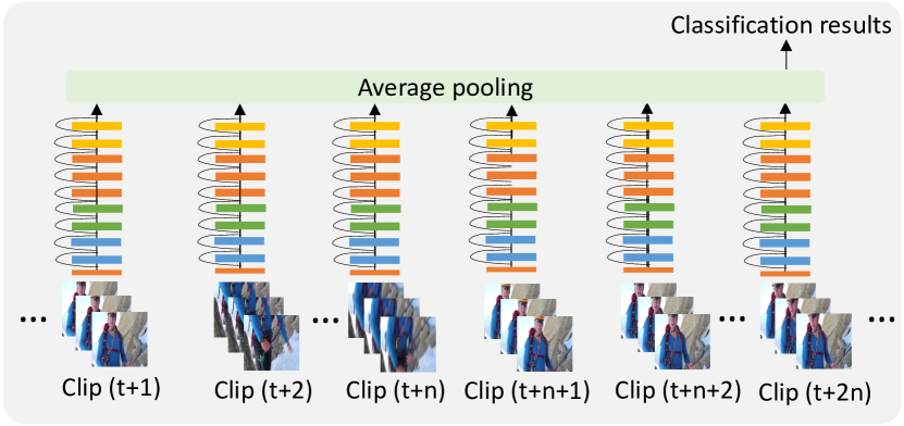
(a) Typical video classification framework for inference.

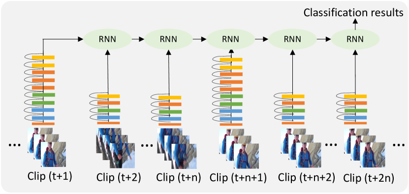
(b) The FASTER framework can process up to 75% of the clips using a much cheaper model without losing accuracy.

Figure 1: (a) Typical video classification framework processes each clip repeatedly with an expensive model; (b) The FASTER framework exploits the combination of expensive and cheap networks for better accuracy/FLOPs trade-offs.

Fig. 1 (a) illustrates the typical framework for video classification. Multiple clips are sampled from a video, and fed to a computationally expensive network to generate predictions for each clip. Clip-level predictions are then aggregated, often by taking the average, to form the final video-level results. To reduce the computational cost, recent efforts have focused on designing more efficient architectures [16] at the clip-level. However, less attention has been paid to the efficiency of the overall framework, including how to aggregate the clip-level predictions over time, since they have a strong temporal structure.

In this work we address the problem of reducing the computational cost of video classification by focusing on the temporal aggregation stage. In particular, we leverage the observation that video data has a strong temporal structure and is highly redundant in time. We argue that it is computationally inefficient to process many video clips close in time with an expensive video model. As adjacent clips are visually similar, computational cost can be saved by processing most of clips with a lightweight network, shown in Fig. 1 (b). A Recurrent Neural Network (RNN) is learned to aggregate the representations from both the expensive and lightweight models. We summarize the contributions of our paper in the following.

First, we propose a novel framework for efficient video classification that we call FASTER for Feature Aggregation for Spatio-TEmporal Redundancy (Fig. 1 (b)). FASTER explicitly leverages the redundancy of video sequences to reduce FLOPs. Instead of processing every clip with an expensive video model, FASTER uses a combination of an expensive model that captures the details of the action, and a lightweight model which captures scene changes over time, avoids redundant computation, and provides a global coverage of the entire video at a low cost. We show that up to 75% of the clips can be processed with a much cheaper model without losing classification accuracy, maintaining the state-of-the-art accuracy with 10$\times$ less FLOPs.

Second, we design a new RNN architecture, namely FAST-GRU, dedicated to the problem of learning to aggregate the representations from different clip models. As shown in our experiments, the prevailing average pooling fails to encode predictions from different distributions. On the contrary, FAST-GRU is capable of learning integration of representations from multiple models for longer periods of time than popular RNNs, such as GRU [8] and LSTM [15]. Compared with typical GRU, FAST-GRU keeps the spatio-temporal resolution of the feature maps unchanged, whereas GRU collapses the resolution with global average pooling. FAST-GRU also has a channel reduction mechanism for feature compression to reduce the number of parameters and introduce more non-linearity. As a result, the FASTER framework achieves significantly better accuracy/FLOPs trade-offs for video classification.

2 Related Work

Before the deep learning era, hand-crafted features [37, 38, 24, 21, 9] were widely used for action recognition. In this section, we cover related works that apply deep learning for efficient video classification.

Clip-level Classification.

Many efforts in video classification focus on designing models to classify short clips. 3D convolutions [3, 18, 19, 35] are widely adopted for learning spatio-temporal information jointly. While these methods do improve the accuracy, they also dramatically increases computational cost due to expensive 3D convolutions. Recent progress includes factorizing 3D convolution into 2D spatial convolution and 1D temporal convolution [33, 28, 36, 43, 45], and designing new building blocks to learn global information on top of 3D convolution [41, 7]. Another line of research designs two-stream networks [29, 44, 40, 11, 5, 43] that use both RGB and optical flow as input. Though two-stream networks tend to improve the accuracy, accurate optical flow algorithms are often computationally expensive.

Video-level Aggregation.

To aggregate the clip-level predictions, average pooling is the most popular approach and works remarkably well in practice. Besides average pooling, [19] proposed convolutional temporal fusion networks for aggregation. NetVLAD [2] also has been used in [12] for feature pooling on videos. [44] learned a global video representation by max-pooling over the last convolutional layer. [40] proposed the TSN network that divides the video into segments, which are averaged for classification. RNNs are also used for sequential learning in video classification [32, 44, 26]. In contrast with existing work, FAST-GRU aggregates the representations from different models, and aims to leverage spatio-temporal redundancy for efficient video classification.

Towards Efficient Video Classification.

[46] proposed the ECO model for online video understanding, where a 3D network is used to aggregate frame-level features. Recent work [1, 42, 22, 4] tried to reduce the computational cost by either reducing the number of frames that need to be processed, or sampling discriminative clips to avoid redundant computation. The FASTER framework is orthogonal to these approaches. Instead of applying sophisticated sampling strategies, we focus on designing a general framework with a new architecture that can learn to aggregate representations from models of different complexities.

3 Learning to Aggregate

As shown in Fig. 1 (b), FASTER is a general framework to aggregate expensive and lightweight representations from different clips. In this section ,we investigate how to learn the temporal structure of clips, aggregate diverse representations to reduce computational cost. We first formulate the problem of learning to aggregate, and introduce the FAST-GRU architecture for aggregation. We then describe other aggregation operators used for comparison and the backbones for extracting the expensive and lightweight representations.

3.1 Problem Formulation

Given a sequence of $N$ clips from a video, we denote their feature representations as $\mathbf{x}_{t}$, where $t\in[0\dots N-1]$. The problem of learning to aggregate can be formulated as:

$$\mathbf{o}_{t}=f(\mathbf{o}_{t-1},\mathbf{x}_{t}),t\in[1\dots N-1],$$ (1)

where $\mathbf{o}_{t-1}$ encodes the historical information before the current clip $\mathbf{x}_{t}$, and $\mathbf{o}_{0}$ equals to $\mathbf{x}_{0}$. Note that Eq. 1 is exactly a recurrent neural network. All previous features $\mathbf{x}_{0}$, $\mathbf{x}_{1}$, …, $\mathbf{x}_{t}$ are recursively encoded into $\mathbf{o}_{t}$. The FASTER framework is suitable for online applications, which requires to provide classification results at any time.

Note also FASTER does not make any assumption about the form of $\mathbf{x}_{t}$. In this paper, we use the feature map from the last convolutional layer of the clip models, which is a tensor of shape $l\times h\times w\times c$, as shown in Fig. 2. $l$ is the temporal length of $\mathbf{x}_{t}$, whereas $h\times w$ is the spatial resolution and $c$ is the number of channels. At any time $t$, $\mathbf{x}_{t}$ can come from either the expensive or lightweight model.

Once all the features are aggregated, we apply global average pooling to $\mathbf{o}_{N-1}$, then feed it to a fully-connected layer, which is trained with SoftMax loss to generate classification scores.

3.2 FAST-GRU

To implement the aggregation function in Eq. 1, we propose the FAST-GRU architecture shown in Fig. 2 (b). While FAST-GRU is based on GRU, we highlight their differences in the following.

3D Convolutional RNN.

RNNs are usually used to model a sequence of inputs represented as 1D feature vectors. These feature vectors can be extracted by applying global average pooling on convolutional feature maps. While these representations are very compact, they do not contain any spatio-temporal information due to pooling. The FASTER framework requires the RNN to handle representations generated by different models. Thus keeping the spatio-temporal resolution of the feature maps may lead to better performance for aggregation. We empirically show that incorporating spatio-temporal information is beneficial for long sequence modeling, which has been largely ignored in recent video pooling methods based on RNNs.

Instead of applying a fully-connected layer to the pooled 1D features, we use a 3D $1\times 1\times 1$ convolution and keep the original resolution of the feature maps in state transitions, as shown in Fig. 2 (b). The matrix multiplication in gating functions is also replaced with 3D $1\times 1\times 1$ convolutions, which enable feature gating in each spatio-temporal location.

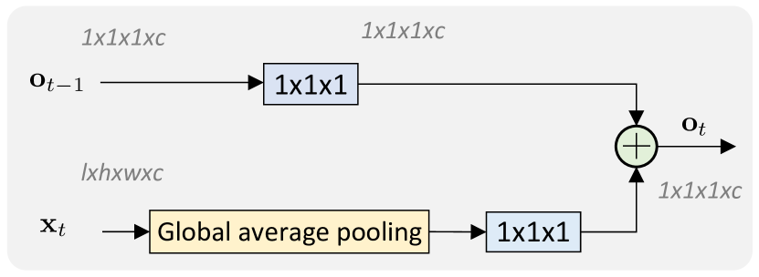
(a) Concat

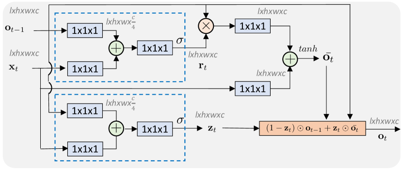
(b) FAST-GRU

Figure 2: (a) The “Concat” baseline simply concatenates $\mathbf{x}_{t}$ with $\mathbf{o}_{t-1}$; (b) Unlike typical GRU collapses the resolution of $\mathbf{x}_{t}$ with global average pooling, FAST-GRU keeps the resolution of $\mathbf{x}_{t}$ to learn spatio-temporal information. We also introduce bottleneck structures (in dash rectangles) in the gate functions to reduce the number of parameters and increase non-linearity.

Bottleneck Gating.

In RNNs, the importance of the current input $\mathbf{x}_{t}$ is decided by a subnetwork conditioned on the historical information encoded in $\mathbf{o}_{t-1}$. The subnetwork learns to combine the state $\mathbf{o}_{t-1}$ and input $\mathbf{x}_{t}$ with different gating mechanisms. Different gates are designed for different functionality for sequential modeling in RNNs. Here we first briefly describe the original GRU architecture, then introduce the bottleneck gating mechanism we proposed.

In GRU, the subnetwork first concatenates $\mathbf{x}_{t}$ and $\mathbf{o}_{t-1}$, then project them to a vector of the same dimension, i.e., the number of channels $c$. There are two gates in GRU, i.e., the read gate $\mathbf{r}$ and update gate $\mathbf{z}$, which are defined as

$$\mathbf{r}_{t} =\sigma(\mathbf{G}_{rx}\mathbf{x}_{t}+{\mathbf{G}_{ro}\mathbf{o}_{t-1}}),$$ (2)

$$\mathbf{z}_{t} =\sigma(\textstyle{\mathbf{G}_{zx}\mathbf{x}_{t}+{\mathbf{G}_{zo}\mathbf{o}_{t-1}}}),$$

where $\mathbf{G}_{*}$ are $c\times c$ matrices, and $\sigma$ is the sigmoid function. After the calculation of $\mathbf{r}_{t}$ and $\mathbf{z}_{t}$, The output of GRU is

$$\bar{\mathbf{o}_{t}} =\textstyle{\tanh(\mathbf{V}_{\bar{o}}\mathbf{x}_{t}+{\mathbf{V}_{\bar{o}}(\mathbf{r}_{t}\odot\mathbf{o}_{t-1})})},$$ (3)

$$\mathbf{o}_{t} =\textstyle{(1-\mathbf{z}_{t})\odot\mathbf{o}_{t-1}+\mathbf{z}_{t}\odot\bar{\mathbf{o}_{t}}},$$

where $\mathbf{V}_{*}$ are $c\times c$ matrices, and $\odot$ represents element-wise multiplication. Both $\mathbf{G}_{*}$ and $\mathbf{V}_{*}$ are learnable parameters.

Inspired by ResNet [14], we introduce additional bottleneck structures to increases the expressiveness of the subnetwork in FAST-GRU, shown in the dash rectangles of Fig. 2 (b). In the bottleneck layer, $\mathbf{x}_{t}$ and $\mathbf{o}_{t-1}$ are projected to a lower dimensional feature space after concatenation. This compresses the number of channels to reduce parameters and introduces more non-linearity. The compressed features are then recovered to the original dimension $c$ with another projection. In practice, channel compression is implemented by $1\times 1\times 1$ convolution to reduce the dimension by a factor of $r$. After that, there is an ReLU followed by $1\times 1\times 1$ convolution to recover the dimensionality. The read and update gates of FAST-GRU are defined as:

$$\mathbf{r^{\prime}}_{t} =\text{ReLU}(\mathbf{U}_{rx}*\mathbf{x}_{t}+{\mathbf{U}_{ro}*\mathbf{o}_{t-1}}),$$ (4)

$$\mathbf{z^{\prime}}_{t} =\text{ReLU}(\textstyle{\mathbf{U}_{zx}*\mathbf{x}_{t}+{\mathbf{U}_{zo}*\mathbf{o}_{t-1}}}),$$

$$\mathbf{r}_{t} =\textstyle{\sigma(\mathbf{W}_{r^{\prime}}*\mathbf{r^{\prime}})},$$

$$\mathbf{z}_{t} =\textstyle{\sigma(\mathbf{W}_{z^{\prime}}*\mathbf{z^{\prime}})},$$

where $\mathbf{U}_{*}$ are $1\times 1\times 1$ convolutions to compress the number of channels by a factor of $r$, and $\mathbf{W}_{*}$ are $1\times 1\times 1$ convolutions to recover the dimensionality. Our gates are generated by taking the jointly compressed features $\mathbf{r}_{t}^{\prime}$ and $\mathbf{z}_{t}^{\prime}$, which enables more powerful gating for feature aggregation. We empirically set $r$ to be $4$, which gives good results in our experiments.

3.3 Other Aggregation Operator Variants

Besides FAST-GRU, we also consider other baselines for the learning-to-aggregate problem for a comprehensive comparison. We detail each baseline in the following.

Average pooling is the most popular approach for aggregation. Despite its simplicity, it performs remarkably well in practice. In the context of our FASTER framework, we just average the classification scores from each clip regardless of whether the scores are generated by the expensive or lightweight model. The concat baseline is illustrated in Fig. 2(a), where $\mathbf{x}_{t}$ and $\mathbf{o}_{t-1}$ are concatenated together, and then projected to a joint feature space. It is defined as:

$$f(\mathbf{o}_{t-1},\mathbf{x}_{t})=\text{ReLU}(\text{BN}(\mathbf{W}\mathbf{o}_{t-1}+\mathbf{U}\mathbf{x}_{t})),$$ (5)

where $\mathbf{W}$ and $\mathbf{U}$ are learnable parameters. Batch normalization [17] and ReLU are also applied in the concat baseline to further improve the performance.

Popular RNNs such as LSTM [15] and GRU [8] are the most related baselines. These are the go-to methods for tasks that involve sequential modeling [34], such as language or speech. For the LSTM baseline, we use the variant that consists of three gates and an additional cell between time steps [13]. LSTM has a forget gate that can reset the history for the current input $\mathbf{x}_{t}$. For video classification, this could be useful in the case of different camera shots or unrelated actions. The GRU baseline we used has two gates, i.e., the read and update gate as we described in the previous section. The state transition function uses the update gate to perform a weighted average of the historical state $\mathbf{o}_{t-1}$ and the current input $\mathbf{x}_{t}$.

3.4 Clip-level Backbones

FASTER is a general framework and does not make any assumption about the underlying clip-level backbones. We can potentially choose any popular networks, such as I3D [5], R(2+1)D [36] or non-local network [41]. We implement FASTER based on R(2+1)D because it is one of the state-of-the-art methods, and its Github repository provides a family of networks that can be used as the expensive and lightweight models. In particular, we choose R(2+1)D with 50 layers as the expensive model, and R2D with 26 layers as the lightweight model, as detailed in Table 1.

Comparing with the original R(2+1)D, we make two changes to further improve its performance. First, we replace convolutional blocks with bottleneck blocks, which have been widely used in the family of ResNet architectures and shown to both reduce computational cost and improve accuracy. Second, we insert a max-pooling layer after $\mathbf{conv}_{1}$, which enables R(2+1)D to support a spatial resolution of $224\times 224$ without significantly increasing its FLOPs.

For the lightweight R2D model, bottleneck layers are used in the same way as R(2+1)D. To reduce the FLOPs of R2D, a temporal stride of 8 is used in $\mathbf{conv}_{1}$, which effectively reduces the temporal length of the clip by a factor of 8. Unlike R(2+1)D, R2D only has 26 layers to further reduce the computational cost.

To integrate R(2+1)D-50 and R2D-26 in FASTER, we simply use the two backbones as feature extractors. In Table 1, the output from res₅ generates a feature map of size $\frac{L}{8}\times 7\times 7\times 2048$, which is used as input $\mathbf{x}_{t}$ to the RNNs.

Layers	R2D-26	R(2+1)D-50	Output sizes $L$$\times$$H$$\times$$W$
conv1	8$\times$7$\times$7, 64	1$\times$7$\times$7, 45, stride 1,2,2	$\begin{array}[]{c}\text{\emph{R2D}}:\text{{$\frac{L}{8}$}$\times$112$\times$112}\\[1.00006pt] \text{\emph{R(2+1)D}}:\text{{$L$}$\times$112$\times$112}\end{array}$
	stride 8, 2, 2	3$\times$1$\times$1, 64, stride 1,1,1
pool1	1$\times$3$\times$3 max		$\begin{array}[]{c}\text{\emph{R2D}}:\text{{$\frac{L}{8}$}$\times$56$\times$56}\\[1.00006pt] \text{\emph{R(2+1)D}}:\text{{$L$}$\times$56$\times$56}\end{array}$
	stride 1, 2, 2
res2	$\left[\begin{array}[]{c}\text{{1$\times$1$\times$1}, {64}}\\ \text{1$\times$3$\times$3, {64}}\\ \text{1$\times$1$\times$1, {256}}\end{array}\right]$$\times$2	$\left[\begin{array}[]{c}\text{{1$\times$1$\times$1}, {64}}\\ \text{1$\times$3$\times$3, 144}\\ \text{3$\times$1$\times$1, {64}}\\ \text{1$\times$1$\times$1, {256}}\end{array}\right]$$\times$3	$\begin{array}[]{c}\text{\emph{R2D}}:\text{{$\frac{L}{8}$}$\times$56$\times$56}\\[1.00006pt] \text{\emph{R(2+1)D}}:\text{{$L$}$\times$56$\times$56}\end{array}$
res3	$\left[\begin{array}[]{c}\text{{1$\times$1$\times$1}, {128}}\\ \text{1$\times$3$\times$3, {128}}\\ \text{1$\times$1$\times$1, {512}}\end{array}\right]$$\times$2	$\left[\begin{array}[]{c}\text{{1$\times$1$\times$1}, {128}}\\ \text{1$\times$3$\times$3, 288}\\ \text{3$\times$1$\times$1, {128}}\\ \text{1$\times$1$\times$1, {512}}\end{array}\right]$$\times$4	$\begin{array}[]{c}\text{\emph{R2D}}:\text{{$\frac{L}{8}$}$\times$28$\times$28}\\[1.00006pt] \text{\emph{R(2+1)D}}:\text{{$\frac{L}{2}$}$\times$28$\times$28}\end{array}$
res4	$\left[\begin{array}[]{c}\text{{1$\times$1$\times$1}, {256}}\\ \text{1$\times$3$\times$3, {256}}\\ \text{1$\times$1$\times$1, {1024}}\end{array}\right]$$\times$2	$\left[\begin{array}[]{c}\text{{1$\times$1$\times$1}, {256}}\\ \text{1$\times$3$\times$3, 576}\\ \text{3$\times$1$\times$1, {256}}\\ \text{1$\times$1$\times$1, {1024}}\end{array}\right]$$\times$6	$\begin{array}[]{c}\text{\emph{R2D}}:\text{{$\frac{L}{8}$}$\times$14$\times$14}\\[1.00006pt] \text{\emph{R(2+1)D}}:\text{$\frac{L}{4}$$\times$14$\times$14}\end{array}$
res5	$\left[\begin{array}[]{c}\text{{1$\times$1$\times$1}, {512}}\\ \text{1$\times$3$\times$3, {512}}\\ \text{1$\times$1$\times$1, {2048}}\end{array}\right]$$\times$2	$\left[\begin{array}[]{c}\text{{1$\times$1$\times$1}, {512}}\\ \text{1$\times$3$\times$3, 1152}\\ \text{3$\times$1$\times$1, {512}}\\ \text{1$\times$1$\times$1, {2048}}\end{array}\right]$$\times$3	$\begin{array}[]{c}\text{\emph{R2D}}:\text{{$\frac{L}{8}$}$\times$7$\times$7}\\[1.00006pt] \text{\emph{R(2+1)D}}:\text{$\frac{L}{8}$$\times$7$\times$7}\end{array}$
global average pooling, fc

Table 1: Clip-level backbones for extracting the expensive and lightweight representations. The FLOPs of R(2+1)D-50 is about 10$\times$ of R2D-26.

4 Experimental Setups

In this section, we describe the experimental setups, i.e., the datasets, training and test protocols for both the clip-level backbones and FASTER framework.

Datasets.

We choose the Kinetics [20] dataset as the major testbed for FASTER. Kinetics is among the most popular datasets for video classification. To simplify, all reported results on Kinetics are trained from scratch, without pre-training on other datasets (e.g., Sports1M or ImageNet). Kinetics has 400 action classes and about 240K training videos. We report top-1 accuracy on the validation set as labels on the testing set is not public available. We also report results on UCF-101 [31] and HMDB-51 [23]. These datasets are much smaller, thus we use Kinetics for pre-training and report mean accuracy on three testing splits.

Model	Input	Video$@$1	GFLOPs$\times$Clips
R2D-26	8-frames	63.3	3.2$\times$32
	16-frames	65.5	6.0$\times$16
	32-frames	66.7	12.7$\times$8
R(2+1)D-50	8-frames	70.1	30.0$\times$32
	16-frames	72.3	60.0$\times$16
	32-frames	74.5	119.9$\times$8

Table 2: Accuracy of clip-level backbones on Kinetics. The significant performance gap between the two backbones offers a great opportunity to explore better accuracy/FLOPs trade-offs when combining them.

Due to limited GPU memory, we train the FASTER framework in a two-stage process. First, two clip-level backbones are trained by themselves separately. In the second stage, two backbones are fixed and we train different RNNs using the feature maps extracted by the backbones.

Setups for clip-level backbones.

We mostly follow the procedure in [36] to train the clip-level backbones except two changes. First, we scale the input video whose shorter side is randomly sampled in [256, 320] pixels, following [41, 30]. Second, we adopt the cosine learning rate schedule [27]. During training, we randomly sample $L$ consecutive frames from a given video. For testing, we uniformly sample $N$ clips to cover the whole video, and average pool the classification scores of each clip, as shown in Table 2. We fix the total number of frames processed to be 256, i.e., $N\times L=256$. As the average length of Kinetics videos is about 10 seconds in 30 FPS, 256 frames give us enough coverage over the whole video. We only use RGB frames as input as computing optical flow can be very expensive.

Setups for learning to aggregate.

To train different RNNs for learning to aggregate, we randomly sample $N$ clips, and each clip has $L$ consecutive frames. As mentioned above, the clip-level backbones are fixed in the second stage due to limited GPU memory. The initial state $\mathbf{o}_{0}$ is set to be the features from the first clip $\mathbf{x}_{0}$. The training procedure is similar to the first stage except we train much fewer epochs. For testing, the $N$ clips are uniformly sampled to cover the whole video.

Model	Number of Clips
	2	4	8	16	32
Avg. pool	60.7	63.9	64.2	64.0	63.8
Concat	61.6	65.9	66.3	62.3	58.2
LSTM	61.3	66.2	66.3	66.3	64.7
GRU	61.1	65.6	66.5	66.1	65.8
FAST-GRU	61.1	65.6	67.2	67.4	67.2

Table 3: Comparison of different architectures for aggregation on Kinetics. The clip length $L$ is 8. For all the methods, only the first clip is processed by the expensive model, and the remaining clips are processed by the lightweight model.

5 Experimental Results

In this section, we demonstrate the advantage of FASTER and discuss accuracy/FLOPs trade-offs in different settings on Kinetics. We also compare FASTER with the state of the art on Kinetics, UCF-101, and HMDB-51.

Accuracy of the backbone architectures.

Table. 2 summarizes the top-1 accuracy of the two clip-level backbones on Kinetics. We consider the clip length $L$ to be 8, 16 or 32 frames, and sample 32, 16 or 8 clips, respectively. This is to ensure that we always process the same number of frames under different settings. Note that the GFLOPs of R(2+1)D-50 is about 10$\times$ of R2D-26, and the accuracy of R(2+1)D-50 is about $7\%$ better than R2D-26. The significant performance gap between the two backbones gives us the opportunity to explore different trade-offs in the following experiments. For the same backbone, longer clip length $L$ often leads to better accuracy. But we can not train R(2+1)D-50 with $L=64$ frames due to GPU memory limit.

FAST-GRU vs. other RNN variants.

We compare the accuracy of different architectures for the learning-to-aggregate problem across a wide range of number of clips ($N=\{2,4,8,16,32\}$). The first clip is always processed with the expensive model and the following $N-1$ clips are processed with the cheap model. We use clip length $L=8$ frames. This allows us to observe the behavior of different architectures in shorter and longer sequences. The results are shown in Table 3. For “Avg. pool”, we simply average the classification scores of all the clips. The performance of “Avg. pool” saturates as more cheap clips are added. Less accurate predictions dominate the final score, since the accuracy of 16 clips (i.e., 64.0%) is quite similar to the accuracy of 32 clips (i.e., 63.8%). This suggests that the expensive representations from the first clip are not fully utilized.

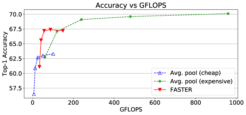
Figure 3: FASTER vs. typical video classification frameworks with average pooling. We show accuracy vs. GFLOPs of different methods as a function of the number of clips. We compare the results of FAST-GRU from Table 3 with average pooling of all expensive (Avg. pool (expensive)) and lightweight models (Avg. pool (cheap)).

“Concat” outperforms “Avg. pool” by 2.1% when $N=8$, showing the benefits of learning temporal structure. However, as $N$ increases, the performance of “Concat” decreases, and by $N=32$, the accuracy is 8.1% lower than $N=8$. This shows that learning to aggregate over a longer time period is difficult. Interestingly, “Concat”, and all recurrent networks have similar performances when the number of clips is small ($N=2,4$), showing that the advantage of RNNs is not evident for short sequences. As the number of clips increases ($N\geq 16$), recurrent networks show their strength in modeling long sequences and perform better than the simple “Concat” baseline.

Of all the methods, FAST-GRU achieves the best performance for long sequences. For example, FAST-GRU outperforms LSTM by 2.5% and GRU by 1.4% when $N=32$. The results show that our proposed FAST-GRU is beneficial for long sequence learning, even when sequence samples come from different distributions.

FASTER vs. average pooling.

How well does the FASTER framework do with respect to the prevailing average pooling? Recall that our main focus is not only to increase accuracy, but also to reduce computational cost. For this, we compare the results of FAST-GRU from Table 3 with the traditional framework (in Fig. 1 (a)), where all clips are cheap (or all clips are expensive) and aggregated with average pooling. These can be considered as the lower and upper bound of the FASTER framework. We plot the GFLOPs vs. accuracy comparisons in Fig. 3. We use clip length $L=8$ frames, and consider the number of clips $N=\{2,4,8,16,32\}$, like Table 3. When $N=4$, it takes 119 GFLOPs for “Avg. pool (expensive)” to achieve 67.1%. FASTER can achieve comparable results with only half the GFLOPs. Comparing with “Avg. pool (cheap)” when $N=16$, FASTER is over 4% better with similar amount of GFLOPs.

Note that there is still an accuracy gap between FASTER and “Avg. pool (expensive)”. In the next experiment, we introduce more expensive clips and study the optimal ratio between the expensive and cheap clips, achieving superior results.

#E :#C	8-frames$\times$32-clips		16-frames$\times$16-clips		32-frames$\times$8-clips
	V$@$1	GFLOPs	V$@$1	GFLOPs	V$@$1	GFLOPs
All E	70.6	$982.4$	72.9	$980.2$	74.9	$979.2$
1:1	70.5	$553.6$	72.9	$552.0$	74.6	$550.4$
1:3	70.1	$339.2$	72.1	$337.6$	73.3	$336.0$
1:7	69.6	$230.4$	71.7	$230.4$	71.3	$228.8$
1:15	69.0	$176.0$	69.9	$176.0$
1:31	67.2	$150.4$

Table 4: Optimal ratio between the expensive and cheap clips. For a fixed number of total frames, we vary the number of clips $N$ and clip length $L$, and measure accuracy and GFLOPs on Kinetics. Empty cells correspond to combinations that are not feasible. “E” denotes the expensive model, while “C” denotes the cheap model. GFLOPs combine the costs of the cheap, expensive and FAST-GRU models together.

Better accuracy/FLOPs trade-offs.

There are three parameters in our framework that affect accuracy and computational cost: the clip length ($L$), the number of clips ($N$), and the proportion of expensive and lightweight clips used as input pattern (#E :#C). We now provide an empirical study of these parameters to achieve the best trade-off. Since we are interested in the behavior of FASTER, we “fix” the input data by keeping the number of frames constant, which spans the entire video. Thus, $L\times N=256$ for all settings. Given $N$ clips, we experiment with input patterns of $1:x$. It is the ratio between the number of expensive clips and cheap clips, $x\in\{1,3,7,15,31\}$. For example, when $x=3$ and $L=16$, there will be 4 expensive clips and 12 cheap clips. Additionally, we evaluate the case where all the inputs are expensive clips ($x=0$).

Results are shown in Table 4. As expected, a higher ratio of expensive models leads to a higher accuracy. For example, when $L=8$, there is a large gap of 1.8% when $x$ goes from $31$ to $15$, with a modest increase of $25.6$ GFLOPs. The gap is less obvious for higher ratios of expensive models. A remarkable observation is that FASTER achieves 70.1% when $x=3$, which is the same accuracy as the average pooling baseline with all expensive clips from Table 2. But FASTER only consumes 35% of its GFLOPs. Even more, for $x=1$, the proposed method outperforms the average pooling baseline in Table 2, at 57% of the cost. This shows the benefit of learning temporal aggregation of hybrid inputs.

We also observe that for a fixed cost, it is often beneficial to use longer clip length $L$. For example, for a fixed proportion of cheap models $x=3$, the accuracy of 32-frames$\times$8-clips is higher than 16-frames$\times$16-clips, and that in turn is considerably higher than 8-frames$\times$32-clips. In other words, it is better to have fewer clips with more frames. However, for higher ratios of cheap clips (e.g., $x=7$), this pattern does not hold.

Model	Time (secs)	GFLOPS	Accuracy
All C (Avg pool)	15.1	101.3	66.7
All E (Avg pool)	75.7	959.3	74.5
FASTER32	35.3	550.4	74.6

Table 5: Comparisons of runtime between different methods. The results of FASTER is reported in the 32-frames$\times$8-clips setting.

#E :#C	32-frames$\times$8-clips
	R(2+1)D-50		R3D-50
	V$@$1	GFLOPs	V$@$1	GFLOPs
All E (Avg. pool)	74.5	959.3	74.4	942.7
1:1 (FAST-GRU)	74.6	550.4	75.3	542.1
1:3 (FAST-GRU)	73.3	336.0	73.9	331.9

Table 6: Compare different architectures as the expensive clip-level backbone. Our FASTER framework can generalize to different architectures, and R3D even performs slightly better than R(2+1)D.

We choose the parameter setting $L=16$ and $x=7$ as the best inexpensive configuration, and call this setting FASTER16 (i.e., $L=16,x=7$). It indicates that it is possible to achieve better performance with shorter clip length $L$, which reflects the importance of learning a good aggregation function. When $L=32$ and $x=1$, the proposed framework achieves 74.6% accuracy with 550.4 GFLOPs. We denote this setting as FASTER32 (i.e., $L=32,x=1$) and it is the best model when the cost is around $\sim$550 GFLOPs .

FASTER also works when all input features come from the same network. When the inputs are all expensive features, FASTER outperforms the average pooling baseline from Table 2 in all settings, with a negligible increase of FLOPs from FAST-GRU.

Runtime vs. FLOPs.

We measure the runtime speed of different methods on a TITAN X GPU with Intel i7 CPU. We sum up the runtime over 100 Kinetics videos. The results are listed in Table 5, which confirms that the theoretical FLOPs are consistent with the runtime for our experiments. The reduction of FLOPs is roughly proportional to the decrease of runtime.

Generalize to different backbones.

Our FASTER framework does not make any assumption about the clip-level backbones. To demonstrate that FASTER can generalize to different backbones, we replace the expensive model, i.e., R(2+1)D-50, with R3D-50 [36] and keep everything else unchanged. In Table 6, R3D even works slightly better than R(2+1)D. Comparing FASTER32 with the average pooling baseline, using R3D leads to a larger improvement of 0.9%.

Model	Top-1	ImageNet pre-train	GFLOPs$\times$clips
I3D [5]	72.1	✓	108$\times$4
S3D [43]	72.2	✓	66.4$\times$N/A
MF-Net [7]	72.8	✓	11.1$\times$50
A2-Net [6]	74.6	✓	40.8$\times$30
S3D-G [43]	74.7	✓	71.4$\times$N/A
NL I3D-50 [41]	76.5	✓	282$\times$30
NL I3D-101 [41]	77.7	✓	359$\times$30
I3D [5]	68.4	-	108$\times$4
STC [10]	68.7	-	N/A$\times$N/A
ARTNet [39]	69.2	-	23.5$\times$250
S3D [43]	69.4	-	66.4$\times$N/A
ECO [46]	70.0	-	N/A$\times$N/A
R(2+1)D-34 [36]	72.0	-	152$\times$115
FASTER16	71.7	-	14.4$\times$16
FASTER32	75.3	-	67.7$\times$8

Table 7: Comparisons to the state-of-the-art methods on Kinetics. The inputs for all the methods are RGB frames. For “GFLOPs $\times$ clips”, we report the cost of a single clip and the number of clips used. “N/A”’ indicates the number of clips are not reported in the paper.

Model	Pre-train		UCF-101	HMDB-51
	I	K
STC [10]	-	✓	95.8	72.6
ARTNet [39]	-	✓	94.3	70.9
ECO [46]	-	✓	93.6	68.4
R(2+1)D-34 [36]	-	✓	96.8	74.5
I3D [5]	✓	✓	95.6	74.8
S3D [43]	✓	✓	96.8	75.9
FASTER32	-	✓	96.9	75.7

Table 8: Comparisons on UCF-101 and HMDB-51. “I” denotes pre-training on ImageNet, while “K” denotes pre-training on Kinetics.

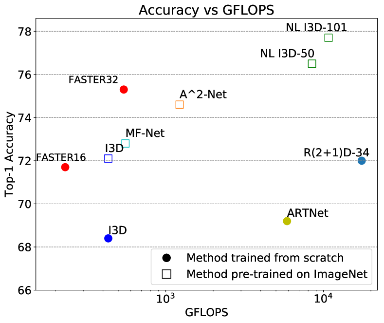
Figure 4: Log-scale GFLOPs vs. accuracy comparisons on Kinetics. In this chart, optimal methods are closer to the top-left corner. The two proposed variants of FASTER are the closest to the corner.

Comparison to state-of-the-art

We now compare the FASTER framework to state-of-the-art methods across three most popular video datasets, i.e., Kinetics, UCF-101 and HMDB-51. We only include methods that use RGB frames as inputs. Results on Kinetics are shown in Table 7. These same numbers are also visualized in terms of accuracy vs. GFLOPs in Fig. 4. Our proposed FASTER framework achieves the best accuracy/GFLOPs trade-offs. This is specially impressive since FASTER is not pre-trained on ImageNet, and the clip-level backbones used are not the most cost effective ones. In this comparison, we use FASTER32 with R3D as its backbone. FASTER32 outperforms R(2+1)D-34 by 3.3% with only 4% of its GFLOPs. FASTER16 outperforms I3D trained from scratch by 3.3% (71.7% vs. 68.4%), using only half of I3D’s cost (432 GFLOPs). Even though we do not leverage pre-training, our framework outperforms all existing pre-trained models except NL-I3D. However, FASTER32 only uses 5% of the GFLOPs of NL-I3D. Our FASTER32 model outperforms $A^{2}$-Net by 0.7%, while the cost is reduced by over 50%. The results validate the effectiveness of our FASTER framework, showing it is promising to leverage the combination of expensive and lightweight models for better accuracy/FLOPs trade-off.

Competitive results are also achieved on UCF-101 and HMDB-51 (Table 8). It shows learning the aggregation function on larger datasets can facilitate the generalization on smaller datasets. The improvements are less profound as the performance on small datasets tends to be saturated.

6 Conclusion

In this paper, we propose a novel framework called FASTER for efficient video classification. To exploit the spatio-temporal redundancy of the video sequence, we combine the representations from both expensive and lightweight models. We propose a recurrent unit called FAST-GRU to learn to aggregate mixed representations. Experimental results show that our FASTER framework has significantly better accuracy/FLOPs trade-offs, achieving the state-of-the-art accuracy with $10\times$ less FLOPs.

References

- [1] H. Alwassel, F. Caba Heilbron, and B. Ghanem. Action search: Spotting actions in videos and its application to temporal action localization. In ECCV, 2018.
- [2] R. Arandjelovic, P. Gronat, A. Torii, T. Pajdla, and J. Sivic. Netvlad: Cnn architecture for weakly supervised place recognition. In CVPR, 2016.
- [3] M. Baccouche, F. Mamalet, C. Wolf, C. Garcia, and A. Baskurt. Sequential deep learning for human action recognition. In International Workshop on Human Behavior Understanding, 2011.
- [4] S. Bhardwaj, M. Srinivasan, and M. M. Khapra. Efficient video classification using fewer frames. In CVPR, 2019.
- [5] J. Carreira and A. Zisserman. Quo vadis, action recognition? a new model and the kinetics dataset. In CVPR, 2017.
- [6] Y. Chen, Y. Kalantidis, J. Li, S. Yan, and J. Feng. A^ 2-nets: Double attention networks. In NIPS, pages 350–359, 2018.
- [7] Y. Chen, Y. Kalantidis, J. Li, S. Yan, and J. Feng. Multi-fiber networks for video recognition. In ECCV, 2018.
- [8] K. Cho, B. van Merrienboer, C. Gulcehre, F. Bougares, H. Schwenk, and Y. Bengio. Learning phrase representations using RNN encoder-decoder for statistical machine translation. In EMNLP, 2015.
- [9] N. Dalal, B. Triggs, and C. Schmid. Human detection using oriented histograms of flow and appearance. In ECCV, 2006.
- [10] A. Diba, M. Fayyaz, V. Sharma, M. M. Arzani, R. Yousefzadeh, J. Gall, and L. Van Gool. Spatio-temporal channel correlation networks for action classification. In ECCV, 2018.
- [11] C. Feichtenhofer, A. Pinz, and A. Zisserman. Convolutional two-stream network fusion for video action recognition. In CVPR, 2016.
- [12] R. Girdhar, D. Ramanan, A. Gupta, J. Sivic, and B. Russell. Actionvlad: Learning spatio-temporal aggregation for action classification. In CVPR, 2017.
- [13] A. Graves. Generating sequences with recurrent neural networks. arXiv preprint arXiv:1308.0850, 2013.
- [14] K. He, X. Zhang, S. Ren, and J. Sun. Deep residual learning for image recognition. In CVPR, 2016.
- [15] S. Hochreiter and J. Schmidhuber. Long short-term memory. Neural Computation, 9(8):1735–1780, 1997.
- [16] A. G. Howard, M. Zhu, B. Chen, D. Kalenichenko, W. Wang, T. Weyand, M. Andreetto, and H. Adam. Mobilenets: Efficient convolutional neural networks for mobile vision applications. arXiv preprint arXiv:1704.04861, 2017.
- [17] S. Ioffe and C. Szegedy. Batch normalization: Accelerating deep network training by reducing internal covariate shift. In ICML, 2015.
- [18] S. Ji, W. Xu, M. Yang, and K. Yu. 3d convolutional neural networks for human action recognition. TPAMI, 2013.
- [19] A. Karpathy, G. Toderici, S. Shetty, T. Leung, R. Sukthankar, and L. Fei-Fei. Large-scale video classification with convolutional neural networks. In CVPR, 2014.
- [20] W. Kay, J. Carreira, K. Simonyan, B. Zhang, C. Hillier, S. Vijayanarasimhan, F. Viola, T. Green, T. Back, P. Natsev, et al. The kinetics human action video dataset. arXiv preprint arXiv:1705.06950, 2017.
- [21] A. Klaser, M. Marszałek, and C. Schmid. A spatio-temporal descriptor based on 3d-gradients. In BMVC, 2008.
- [22] B. Korbar, D. Tran, and L. Torresani. Scsampler: Sampling salient clips from video for efficient action recognition. arXiv preprint arXiv:1904.04289, 2019.
- [23] H. Kuehne, H. Jhuang, E. Garrote, T. Poggio, and T. Serre. Hmdb: a large video database for human motion recognition. In ICCV, 2011.
- [24] I. Laptev. On space-time interest points. IJCV, 2005.
- [25] Y. LeCun, L. Bottou, Y. Bengio, and P. Haffner. Gradient-based learning applied to document recognition. Proceedings of the IEEE, 86(11):2278–2324, 1998.
- [26] Z. Li, K. Gavrilyuk, E. Gavves, M. Jain, and C. G. Snoek. Videolstm convolves, attends and flows for action recognition. CVIU, 166:41–50, 2018.
- [27] I. Loshchilov and F. Hutter. Sgdr: Stochastic gradient descent with warm restarts. arXiv preprint arXiv:1608.03983, 2016.
- [28] Z. Qiu, T. Yao, and T. Mei. Learning spatio-temporal representation with pseudo-3d residual networks. In ICCV, 2017.
- [29] K. Simonyan and A. Zisserman. Two-stream convolutional networks for action recognition in videos. In NIPS, 2014.
- [30] K. Simonyan and A. Zisserman. Very deep convolutional networks for large-scale image recognition. In ICLR, 2015.
- [31] K. Soomro, A. R. Zamir, and M. Shah. UCF101: A dataset of 101 human actions classes from videos in the wild. arXiv preprint arXiv:1212.0402, 2012.
- [32] N. Srivastava, E. Mansimov, and R. Salakhudinov. Unsupervised learning of video representations using LSTMs. In ICML, 2015.
- [33] L. Sun, K. Jia, D.-Y. Yeung, and B. E. Shi. Human action recognition using factorized spatio-temporal convolutional networks. In ICCV, 2015.
- [34] I. Sutskever, O. Vinyals, and Q. V. Le. Sequence to sequence learning with neural networks. In NIPS, 2014.
- [35] D. Tran, L. Bourdev, R. Fergus, L. Torresani, and M. Paluri. Learning spatiotemporal features with 3D convolutional networks. In ICCV, 2015.
- [36] D. Tran, H. Wang, L. Torresani, J. Ray, Y. LeCun, and M. Paluri. A closer look at spatiotemporal convolutions for action recognition. In CVPR, 2018.
- [37] H. Wang, A. Kläser, C. Schmid, and C.-L. Liu. Action recognition by dense trajectories. In CVPR, 2011.
- [38] H. Wang and C. Schmid. Action recognition with improved trajectories. In ICCV, 2013.
- [39] L. Wang, W. Li, W. Li, and L. Van Gool. Appearance-and-relation networks for video classification. In CVPR, 2017.
- [40] L. Wang, Y. Xiong, Z. Wang, Y. Qiao, D. Lin, X. Tang, and L. Van Gool. Temporal segment networks: Towards good practices for deep action recognition. In ECCV, 2016.
- [41] X. Wang, R. Girshick, A. Gupta, and K. He. Non-local neural networks. In CVPR, 2018.
- [42] Z. Wu, C. Xiong, C.-Y. Ma, R. Socher, and L. S. Davis. Adaframe: Adaptive frame selection for fast video recognition. In CVPR, 2019.
- [43] S. Xie, C. Sun, J. Huang, Z. Tu, and K. Murphy. Rethinking spatiotemporal feature learning: Speed-accuracy trade-offs in video classification. In ECCV, 2018.
- [44] J. Yue-Hei Ng, M. Hausknecht, S. Vijayanarasimhan, O. Vinyals, R. Monga, and G. Toderici. Beyond short snippets: Deep networks for video classification. In CVPR, 2015.
- [45] Y. Zhou, X. Sun, Z.-J. Zha, and W. Zeng. Mict: Mixed 3d/2d convolutional tube for human action recognition. In CVPR, 2018.
- [46] M. Zolfaghari, K. Singh, and T. Brox. Eco: Efficient convolutional network for online video understanding. In ECCV, 2018.