Tuning morphology and thermal transport of asymmetric smart polymer blends by macromolecular engineering

Abstract

A grand challenge in designing polymeric materials is to tune their properties by macromolecular engineering. In this context, one of the drawbacks that often limits broader applications under high temperature conditions is their poor thermal conductivity $\kappa$. Using molecular dynamics simulations, we establish a structure-property relationship in hydrogen bonded polymer blends for possible improvement of $\kappa$. For this purpose, we investigate two experimentally relevant hydrogen bonded systems$-$ one system consists of short poly(N-acryloyl piperidine) (PAP) blended with longer chains of poly(acrylic acid) (PAA) and the second system is a mixture of PAA and short poly(acrylamide) (PAM) chains. Simulation results show that PAA-PAP blends are at the onset of phase separation over the full range of PAP monomer mole fraction $\phi_{\rm PAP}$, which intensifies even more for $\phi_{\rm PAP}>0.3$. While PAA and PAP interact with preferential hydrogen bonding, phase separation is triggered by the dominant van der Waals attraction between the hydrophobic side groups of PAP. However, if PAP is replaced with PAM, which has a similar chemical structure as PAP without the hydrophobic side group, PAA-PAM blends show much improved solubility. Better solubility is due to the preferential hydrogen bonding between PAA and PAM. As a result, PAM oligomers act as cross-linking bridges between PAA chains resulting in a three dimensional highly cross-linked network. While $\kappa$ for PAA-PAP blends remain almost invariant with $\phi_{\rm PAP}$, PAA-PAM systems show improved $\kappa$ with increasing PAM concentration and also with respect to PAA-PAP blends. Consistent with the theoretical prediction for the thermal transport of amorphous polymers, we show that $\kappa$ is proportional to the materials stiffness, i.e., the bulk modulus $K$ and sound velocity $v$ of PAA-PAM blends. However, no functional dependence between $\kappa$ and $K$ (or $v$) is observed for the immiscible PAA-PAP blends.

I Introduction

Polymers are ubiquitous in our everyday life, finding a variety of applications ranging from physics to materials science and chemistry to biology [1, 2, 3, 4, 5, 6]. The properties of polymers are intimately linked to large conformational and compositional fluctuations. Because of the molecular flexibility, polymer conformations can be tuned almost at will for desired applications and thus provide a robust platform for advanced functional materials design. However, one of the drawbacks of standard commodity polymeric materials is the poor thermal conductivity $\kappa$ in their amorphous states [7, 8, 9]. This is partially because of rather weak van der Waals interactions dictating polymer properties. Therefore, it is desirable to tune $\kappa$ of polymeric materials, especially when they are used in high temperature environments.

One of the standard protocols to improve $\kappa$ of polymeric materials is blending them with materials having $\kappa$ values exceeding the thermal conductivity of metals, such as carbon based materials [10, 11, 12, 13]. In this context, following the arguments of continuum theory, one should expect to increase $\kappa$ of polymer composites with increasing concentration of the high $\kappa$ guest. Moreover, establishing a tunable structure-function relationship in these composite materials is often difficult because they exhibit large spatial and temporal heterogeneities. Furthermore, a significant improvement in $\kappa$ also requires concentrations of external guest material exceeding their percolation threshold, thus also losing the inherent property and flexibility of the host polymeric systems. Therefore, a more attractive protocol to tune $\kappa$ is to strengthen microscopic interactions within the polymer system itself. Here, smart polymers may serve as ideal candidates.

A polymer is referred to as “smart”, when they exhibit fast responsiveness to a change in their environment in solutions and are typically dictated by hydrogen bonding whose strength typically falls within the range of 4-8 $k_{\rm{}_{B}}T$, thus exceeding significantly the van der Waals pair interactions that are only of the order of less than $k_{\rm{}_{B}}T$ [1, 2, 4, 5]. Therefore, the solvent-free dry states of these hydrogen bonded polymers are dictated by strong inter-polymer interactions. In this context, there is considerable interest to study thermal transport in tunable polymer materials [14, 15, 16], smart hydrogels [17, 18], concentrated polymer solutions [19], and solid polyelectrolytes [20]. In particular, a recent work uses the idea of hydrogen bonding as a tunable interaction to propose a wide range of polymer blends, where a significant increase in $\kappa$ was observed [14]. One of the interesting systems this experiment proposes is an asymmetric blend of poly(N-acryloyl piperidine) (PAP) and poly(acrylic acid) (PAA) with M${}_{\rm w}^{\rm PAA}\gg$ M${}_{\rm w}^{\rm PAP}$, where M_w is the molecular weight. Schematic representations of chemical structures of PAA and PAP are shown in Figures 1(a-b).

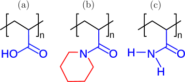
Figure 1: Schematic representations of$-$ (a) poly(acrylic acid) (PAA), (b) poly(N-acryloyl piperidine) (PAP) and (c) poly(acrylamide) (PAM) systems. The length of PAA was chosen as $N_{\ell}^{\rm PAA}=30$, the lengths of PAP and PAM is taken as $3$. Highlighted blue regions are possible groups forming hydrogen bonding, while the black and red regions are hydrophobic in nature.

It was reported that, for a PAP monomer mole fraction $\phi_{\rm PAP}\sim 0.3$, $\kappa$ increases by a factor of about 6$-$7 times with respect to $\kappa\sim 0.25$ Wm^-1K^-1 of pure PAA (or pure PAP) [14]. This increase was attributed to the strong PAA-PAP hydrogen bonding, which also demands as prerequisite that the binary solution of PAA and PAP are fairly miscible. In a separate experimental study, however, it was found that PAA and PAP phase separate, while no variation in $\kappa$ was observed over the full range of $\phi_{\rm PAP}$ [15].

If a system is phase separated, it is expected to show reduced $\kappa$ because of the weakened interfacial interaction between two phase separated regions. However, because of the delicate interplay between the van der Waals and hydrogen bonding interactions in these systems, it is not always straightforward to predict molecular level morphology and its connection to thermal transport, which is the motivation behind this study. To best of our knowledge, there is no theoretical/computational work addressing polymer blends in their dry states for tunable $\kappa$. In this work, we present molecular dynamics simulation results establishing a structure-property relationship in polymer blends. For this purpose, we investigate two experimentally relevant systems$-$ one system is a simulation replica of the PAA-PAP blend reported earlier [14] and the second system consists of a PAA and poly(acrylamide) (PAM) blend, where PAM has a very similar chemical structure as PAP without the hydrophobic carbon ring, see Figure 1(c).

The remainder of the paper is organized as follows: In section II we sketch our methodology. Results and discussions are presented in sections III and finally the conclusions are drawn in section IV.

II Method and model

In this work all-atom molecular dynamics simulations are performed at two stages: the GROMACS 4.6 package [21] was used for the equilibration and structural analysis of the polymer blends, while the LAMMPS package [22] was used for the thermal transport calculations.

GROMACS simulations are performed in the NpT ensemble, where N is the number of particles in a system, p is the isotropic pressure, and T is the temperature. T= 600 K is set for the initial simulations using a Berendsen thermostat with a coupling constant 2 ps. This ensures that the polymer blends are in their melt states. p is kept at 1 bar using a Berendsen barostat with a coupling time of 0.5 ps [23]. Electrostatics are treated using the particle mesh Ewald method [24]. The interaction cutoff for non-bonded interactions is chosen as 1.0 nm. The simulation time step is chosen as $\Delta t=1$ fs and the equations of motion are integrated using the leap-frog algorithm [25]. All bond vibrations are constrained using a LINCS algorithm [26].

We investigate two different polymer systems, namely PAA-PAP and PAA-PAM blends. Configurations consist of a total of 200 chains, where the length of PAA is chosen as $N_{\ell}^{\rm PAA}=30$, while the lengths of both PAP and PAM oligomers are taken as $N_{\ell}^{\rm PAP}$ (or $N_{\ell}^{\rm PAM}$) = 3. In a series of simulations, the PAP monomer mole fractions $\phi_{\rm PAP}$ and PAM monomer mole fractions $\phi_{\rm PAM}$ are varied between $0.0-1.0$, where $\phi_{i}=0.0$ corresponds to pure PAA and $\phi_{i}=1.0$ represents pure PAP or PAM systems. The standard OPLS force field was used for PAA and PAP systems [27]. For PAM we have used modified parameters that were developed by two of us earlier [28]. While both these force fields were previously used for the study of polymers in solution, in the supplementary materials we provide evidence that these force fields are also suitable to study dry polymer films.

After an initial equilibration of 20 ns, production runs are performed for 60 ns and the configurations were saved each 50 fs for the calculation of the structural properties. These simulation runs are at least one order of magnitude larger than the longest relaxation time $\tau\sim 5$ ns of a PAA chain with $N_{\ell}^{\rm PAA}=30$ and T = 600 K, which is estimated using the end-to-end distance auto-correlation function $\left<{\bf R}(t)\cdot{\bf R}(0)\right>\sim e^{-t/\tau}$. During the production runs, observables such as the radial distribution function ${\rm g}_{ij}(r)$ and the number of hydrogen bonds (h$-$bond) for different solution components are calculated. H$-$bond are calculated using the standard geometrical criterion implemented in GROMACS, i.e., a hydrogen bond exists when the donor-acceptor distance is $\leq 0.35$ nm and the acceptor-donor-hydrogen angle is $\leq 30^{\circ}$.

The final configurations from the GROMACS simulations were first quenched down to $T=300$ K and then imported in LAMMPS for $\kappa$ calculations. Note that both pure PAA and PAP have their glass transition temperatures $T_{\rm g}\sim 373$ K [14], while $T_{\rm g}$ of bulk PAM exceeds 430 K [29]. Therefore, without attempting to identify a precise $T_{\rm g}$ value for different blends and following a simple combination rule, one expects $T=300$ K to be well below their corresponding $T_{\rm g}$. This, however, also assumes a priory that the bulk solution is miscible.

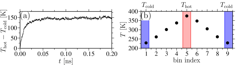
Figure 2: Part (a) shows the time equilibration of temperature difference between the hot $T_{\rm hot}$ and the cold $T_{\rm cold}$ regions of a PAA-PAM blend for $\phi_{\rm PAM}=0.286$. Part (b) shows the steady-state temperature profile with bin index along the $z-$axis of the simulation domain. Note that while we sub-divide simulation domain into eight chunks, nine chunks are shown because of the periodic boundary condition.

For the calculation of $\kappa$, we employ a non-equilibrium method [30]. In this method, a heat flux $J$ through the system is generated over a simulation time $\mathcal{T}$ in the microcanonical ensemble by swapping atomic velocities between a hot and a cold region of the simulation box,

$$J=\frac{1}{2\,A\mathcal{T}}{\sum_{\text{swaps}}\Delta E_{\text{kin}}},$$ (1)

where $\Delta E_{\text{kin }}$denotes the kinetic energy exchanged per swap, $A$ is the cross sectional area perpendicular to the direction of heat flow, and the factor 2 accounts for the two directions of heat flow present in systems with periodic boundaries. As a result of velocity swapping, once the system reaches its steady-state, a temperature gradient $\Delta T/\Delta z$ along the transport direction $z$ can be extracted and the thermal conductivity $\kappa$ is calculated by applying Fourier’s law of heat conduction,

$$\kappa=\frac{J}{\left|\Delta T/\Delta z\right|}.$$ (2)

Here we chose to divide the simulation box into eight slabs of equal width along the $z-$direction. This will lead to at least $\sim 1500$ atoms per slab. Note that when dealing with PAA-PAP blends special care needs to be taken in choosing the slab width because of the phase separation. Velocity swapping was performed between the slowest atom in the center slab and the fastest atom in the slab at the cell boundary. This swapping was performed every 20 fs with $\Delta t=0.2$ fs. After an initial steady-state equilibration for $10^{6}$ time-steps (see Figure 2(a)), the heat flux was computed over a simulation time of $5\cdot 10^{5}$ time-steps. Finally, a linear fit of the temperature profile as a function of slab index was used to calculate $\kappa$ by means of Eq. (2), as shown in Figure 2(b).

We have also attempted to calculate $\kappa$ using the equilibrium Kubo-Green method in LAMMPS [31], which, however, overestimates $\kappa$ by about an order of magnitude. This can be attributed to the heat-flux autocorrelation function routine of the LAMMPS code that only considers pair-wise interactions. Systems with many-body interactions may, therefore, lead to problems in $\kappa$ calculations. More specifically, Kubo-Green should give the same $\kappa$ values as in a non-equilibrium method. This, however, also require to properly accounting angular and dihedral interactions in the all-atom force fields for the heat-flux calculations [32]. This was also identified earlier for the simulations of carbon based materials [33].

III Results and discussions

III.1 Morphology of polymer blends in the melt state

We start our discussion by investigating the molecular level morphologies of PAA-PAP blends at T = 600 K. For this purpose, we calculate pair correlation functions ${\rm g}_{ij}(r)$ between different solution components. Because the properties of these systems are dictated by hydrogen bonding, ${\rm g}_{ij}(r)$ are calculated only between oxygen and hydrogen of PAA and oxygen and nitrogen of PAP, see highlighted blue components in Figure 1. In Figures 3(a-c), we show ${\rm g}_{ij}(r)$ between different monomeric species for two different $\phi_{\rm PAP}$. A closer look at the data for $\phi_{\rm PAP}=0.024$ (black curves in Figures 3(a-c)) reveals two important length scales: (a) The most prominent fluid structure is observed for $r\leq 1$ nm represented by the correlation peaks. (b) ${\rm g}_{ij}(r)\to 1$ for $r\geq 1.5$ nm, which is the typical correlation length in the hydrogen bonded systems [35]. Furthermore, the long tail decay, as observed for $\phi_{\rm PAP}=0.320$ (red curves in Figures 3(a-c)), indicates that the system is at the onset of phase separation.

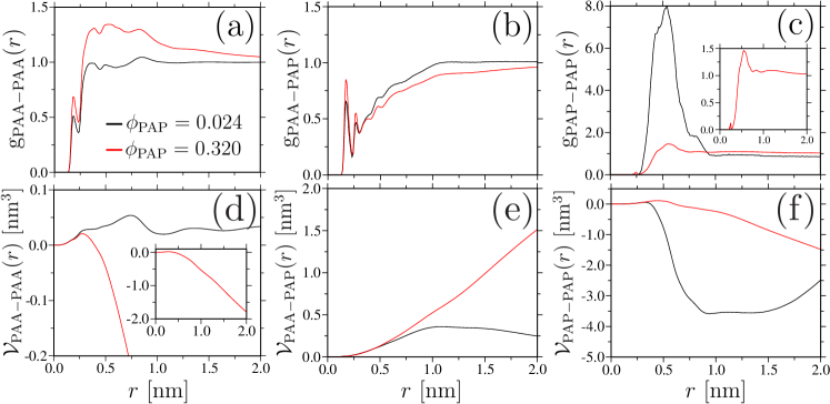
Figure 3: Radial distribution functions ${\rm g}_{\rm ij}(r)$ between three different monomeric pairs in polymer blends consisting of poly(N-acrylyol piperidine) (PAP) and poly(acrylic acid) (PAA): (a) PAA-PAA, (b) PAA-PAP, and (c) PAP-PAP. Results are shown for two different PAP monomer molar fractions $\phi_{\rm PAP}$ under their melt states at a temperature of T$=600$ K and ambient pressure. Number of repeat units of PAP and PAA was chosen to be 3 and 30, respectively. For the calculation of ${\rm g}_{\rm ij}(r)$, we only consider oxygens and hydrogen of PAA and oxygen and nitrogen of PAP, as highlighted by blue species in Figure 1. Inset in part (c) is the enlarged view of ${\rm g}_{\rm PAP-PAP}(r)$ for $\phi_{\rm PAP}=0.320$ highlighting first peak height. Parts (d-f) shows the cumulative integral of the second virial coefficient $\mathcal{V}_{ij}(r)$ between solution components. Inset in part (d) highlights the diverging $\mathcal{V}_{\rm PAA-PAA}(r)$ for $\phi_{\rm PAP}=0.320$.

The pair correlation function ${\rm g}_{\rm ij}(r)$ not only gives information about the pairwise solution structure, it also provides information about solution thermodynamics via the second virial coefficient,

$$\mathcal{V}_{ij}(r) = 2\pi\int_{0}^{\infty}\left[1-e^{-{\rm V}_{ij}(r)/k_{\rm B}T}\right]r^{2}dr$$ (3)

$$= 2\pi\int_{0}^{\infty}\left[1-{\rm g}_{ij}(r)\right]r^{2}dr.$$

This assumes $V_{ij}(r)=-k_{\rm B}T\ln\left[{\rm g}_{ij}(r)\right]$ [34]. In polymer science, $\mathcal{V}_{ij}$ is also known as the excluded volume and is defined by the plateau value of the cumulative integral ${\mathcal{V}}_{ij}(r)$ for $r$ value above the correlation length. For example, the interaction between $i$ and $j$ is repulsive when $\mathcal{V}_{ij}>0$ and attractive when $\mathcal{V}_{ij}<0$. When $\mathcal{V}_{ij}=0$, the long range energetic attraction gets exactly canceled by the short range entropic repulsion, which is also known as the “so called” $\Theta-$point (or a critical point) that is dictated by large diverging fluctuations. Note that the convergence of ${\mathcal{V}}_{ij}(r)$ for large $r$ values suffers from severe system size effects, especially for multi-component solutions [35]. Moreover, in this study we have chosen system sizes to be large enough to avoid system size effects.

Figures 3(d-f) show ${\mathcal{V}}_{ij}(r)$ for three different pairs of PAA-PAP blends. For $\phi_{\rm PAP}=0.024$ it can be appreciated that both PAA-PAA and PAA-PAP interactions are weak, while the PAP-PAP interaction is highly attractive as indicated by large negative value of ${\mathcal{V}}_{\rm PAP-PAP}(r)$. Almost equal preference for the interactions between PAA-PAA and PAA-PAP are not surprising, given that these species are hydrogen bonded. Moreover, the dominant contribution of the PAP-PAP interaction comes from the van der Waals interaction between the hydrophobic side ring of PAP (highlighted by red in Figure 1). We also want to emphasize that even when van der Waals interaction between two individual particles is rather weak (i.e., less than $k_{\rm B}T$), collectively they may result in several $k_{\rm B}T$ of interaction strength, as seen here for the PAP-PAP coordination. Furthermore, a diverging ${\mathcal{V}}_{\rm PAA-PAP}(r)$ for $\phi_{\rm PAP}=0.320$ further indicates phase separation in PAA-PAP blend.

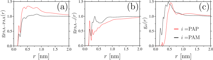
Figure 4: Radial distribution function ${\rm g}_{\rm ij}(r)$ between three different monomeric pairs in polymer blends for two different systems. One system is a blend of trimer of poly(N-acrylyol piperidine) (PAP) is blended in with poly(acrylic acid) (PAA) with length $N_{\ell}^{\rm PAA}=30$ (red curves) and the second systems is a mixture of PAA of same length with trimer of poly(acrylamide) (PAM) (black curves). The data is shown for 0.320 monomer mole fraction of shorter species, T$=600$ K and ambient pressure. Parts (a-c) show$-$ PAA-PAA, PAA-$i$ and $i-i$ structures, with the unit $i$ can either be PAP or PAM as specified in the legend.

Solution processing of polymers with distinct nanoscopic interfaces, as in the case of phase separation, and their use for tunable thermal, mechanical, optical and/or rheological properties is always a paramount challenge. Therefore, it is desirable to have better miscible systems for advanced applications. In this context, since the phase separation in a PAA-PAP blend is dictated by interactions between the hydrophobic side groups of PAP, one possibility to improve solubility of a blend might be to remove the side carbon ring in a PAP monomer structure. Here PAM may serve as an ideal candidate (see Figure 1(c)). PAM is an easy replacement because it has a similar monomer structure as PAP without the carbon ring. Additionally, PAM is a water soluble polymer [28], unlike PAP [15] that is hydrophobic. The added advantage of using PAM arises from more possibility of hydrogen bonds in comparison to PAP, thus forming stronger contacts between two particles.

In Figure 4 we show a component-wise ${\rm g}_{ij}(r)$ for two different blends. It can be appreciated that the system shows better tail convergence for PAA-PAM systems in comparison to PAA-PAP blends, i.e., ${\rm g}_{ij}(r)=1$ around the correlation length of 1.5 nm. This indicates a much better solubility in the system, as expected by the structural tuning of the monomer units discussed in the preceding paragraph.

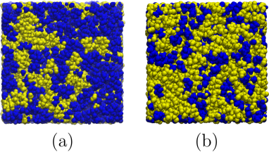
Figure 5: Space filling representation of the simulation snapshots for PAA-PAP blend part(a) and PAA-PAM blend part(b). The data is shown for 0.320 monomer mole fraction of shorter species, T$=600$ K and ambient pressure. Yellow spheres represent PAA atoms and blue spheres show PAP atoms (panel (a)) and PAM atoms (panel (b)).

An illustration of molecular level morphologies in two blends are shown in Figure 5. It is evident that PAA-PAM is more homogeneous, while PAA-PAP shows distinct islands.

Having discussed morphologies of smart polymer blends, we now move to understand the correlation between morphologies and $\kappa$ in the dry states of these systems.

III.2 Hydrogen bonding and thermal transport in polymer blends below the glass transition temperature

Hydrogen bonding (H$-$bond) is an important molecular level interaction in these smart materials [1, 2, 4, 5, 36]. Therefore, we now investigate possible H$-$bonds between different solution species. In Figure 6, we show the fraction of H$-$bonds $\phi^{\rm H-bond}_{{\rm PAA}-i}$ between PAA and the other species $i$, which can be either PAP or PAM. In a nutshell, if $\phi^{\rm H-bond}_{{\rm PAA}-i}$ is above the blue line (i.e., linear extrapolation between two concentrations with unity slope and zero intercept), there is an excess of H$-$bonds for a given monomer mole fraction $\phi_{i}$.

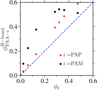
Figure 6: Fraction of hydrogen bond $\phi^{\rm H-bond}_{{\rm PAA}-i}$ between cross components of two polymer blends (PAA-PAP and PAA-PAM blends) as a function of monomer mole fraction $\phi_{i}$, with $i$ can either be PAP or PAM. Blue dashed line is a linear interpolation between two values of $\phi_{i}$ with unit slope and zero intercept. The data is shown for the dry state of polymer blends for T$=300$ K and ambient pressure.

For the PAA-PAP systems (red stars in Figure 6) it can be seen that even when PAA and PAP phase separate, there is an excess concentration of H$-$bonds between PAA and PAP. This is because both PAA and PAP form isolated islands having their side groups dangling within the interface between two phase separated regions. Therefore, they can still facilitate interfacial H$-$bonds acting as adhesive contacts between two islands. Here it is also worth mentioning that the phase separation, as observed in PAA-PAP case, may not be a standard spinodal decomposition [37]. More specifically, the PAP oligomers are glued together by their hydrophobic contacts leading to the phase separation. To better understand the thermodynamic origin of the phase separation in PAA-PAP blends a more detailed investigation is needed, which is beyond the scope of the present study. Furthermore, we expect these small islands to coarsen over longer simulation times even if they are driven by weak surface tension. Moreover, our simulations already show a clear signature that the PAA-PAP systems are at the onset of phase separation (see Figure 5).

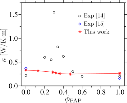
Figure 7: Thermal transport coefficient $\kappa$ for PAA-PAP blend as a function of PAP monomer mole fraction $\phi_{\rm PAP}$. The data is shown for the dry state (below the glass transition temperature) of polymer blends for temperature T$=300$ K and ambient pressure. A typical error of 10% is estimated from five different $\kappa$ calculations using different random seeds during microcanonical simulations. For comparison, we have also included experimentally reported $\kappa$ values obtained for PAA-PAP blends [14] and the homopolymer data for pure PAA ($\phi_{\rm PAP}=0.0$) and for pure PAP ($\phi_{\rm PAP}=1.0$) [15].

Having two glued regions, as in the case of PAA-PAP blends, does not necessarily mean that one can also expect to have a variation in $\kappa$ within the intermediate mixing ratios of $\phi_{\rm PAP}$. Instead the overall behavior is expected to be dominated by $\kappa$ values of two individual components, with rather weak interfacial interactions. Therefore, following the simple mixing rule, one should only expect a smooth interpolation of $\kappa$ between two pure phases of PAA and PAP. Indeed, as shown by the simulation data in Figure 7 (red stars), $\kappa$ varies rather monotonically with $\phi_{\rm PAP}$. It should also be noted that$-$ for the pure phases of PAA and PAP, our calculated values $\kappa\sim 0.32$ Wm^-1K^-1 (for $\phi_{\rm PAP}=0.0$) and $\kappa\sim 0.27$ Wm^-1K^-1 (for $\phi_{\rm PAP}=1.0$) are in good agreement with the experimental data, see Figure 7 [14, 15]. For example, one experiment reported $\kappa\sim 0.22$ Wm^-1K^-1 (for $\phi_{\rm PAP}=0.0$) and $\kappa\sim 0.20$ Wm^-1K^-1 (for $\phi_{\rm PAP}=1.0$) [14], while another set of experimental data reported $\kappa\sim 0.37$ Wm^-1K^-1 (for $\phi_{\rm PAP}=0.0$) and $\kappa\sim 0.16$ Wm^-1K^-1 (for $\phi_{\rm PAP}=1.0$) [15]. Furthermore, our simulation data for intermediate mixing ratios of $\phi_{\rm PAP}$ is in clear contradiction with one set of earlier published experimental data [14] (see the data set corresponding to the black circles in Figure 7), while it is in agreement with another set of experimental observations [15].

For the PAA-PAM system, we observe a higher $\phi^{\rm H-bond}_{{\rm PAA}-{\rm PAM}}$ (black filled circles in Figure 6). This excess is also coupled with an improvement in $\kappa$ for PAA-PAM blends in comparison to PAA-PAP systems, see corresponding data with black filled circles in Figure 8(a).

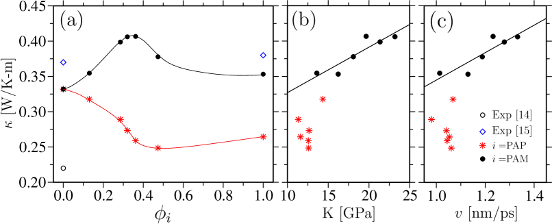
Figure 8: Part (a) shows comparative data of thermal transport coefficient $\kappa$ obtained from simulations for PAA-PAM and PAA-PAP blends as a function of monomer mole fraction $\phi_{i}$, with $i$ can either be PAP or PAP. The data is shown for the dry state (below glass transition temperature) of polymer blends for temperature T$=300$ K and ambient pressure. A typical error of 10% is estimated from five different $\kappa$ calculations using different random seeds during microcanonical simulations. For comparison, we have also included experimentally reported $\kappa$ values obtained for pure PAA ($\phi_{\rm PAP}=0.0$) [14, 15] and pure PAM ($\phi_{\rm PAP}=1.0$) [15]. Lines are drawn to guide the eye. Parts (b-c) show $\kappa$ as a function of bulk modulus $K$ and sound velocity $v=\sqrt{K/\rho}$ calculated for both blends, where $\rho$ is the mass density. The black solid lines are linear fits to the PAA-PAM data.

The improvement of $\kappa$ for PAA-PAM as compared to PAA-PAP is not surprising, given that PAA and PAM are fairly miscible because of preferential H$-$bonding between PAA and PAM (see Figure 4 and Figure 6). Moreover, to further investigate the tunability of $\kappa$, we have also looked into the minimal thermal conductivity model [15, 38, 39]. Within this theory for amorphous polymer (as in our cases), $\kappa$ relates directly to the materials stiffness, thus is also related to the glass transition temperature $T_{\rm g}$ of amorphous systems [14] and the sound wave velocity $v$. The higher the stiffness (or $v$), the larger the corresponding $\kappa$ [40]. In this context and for the pure phases of PAA, PAP and PAM, we find that our calculated $\kappa$ values follow the trend $\kappa^{\rm PAM}>\kappa^{\rm PAA}>\kappa^{\rm PAP}$ and are consistent with $T_{\rm g}^{\rm PAM}>T_{\rm g}^{\rm PAA}>T_{\rm g}^{\rm PAP}$, see the supplementary Fig. 1 and Table I. Furthermore, the sound velocity can be estimated using the Newton-Laplace equation $v=\sqrt{K/\rho}$, where $\rho$ is the mass density and $K$ is the bulk modulus. Here, volume fluctuations are used to calculate $K$ from NpT simulations using the expression

$$K=k_{\rm B}T\frac{\left<V\right>}{\left<V^{2}\right>-\left<V\right>^{2}}.$$ (4)

As expected from the theory [15, 38, 39] and observed earlier in experiments [15], our simulation data for PAA-PAM blends show that $\kappa$ is proportional to $K$ and $v$, see black symbols in Figures 8(b-c). Additionally, the lack of correlation between $\kappa$ and $K$ (or $v$) for PAA-PAP is due to the phase separation in the systems, see red symbols in Figures 8(b-c).

From the $K$ and $v$ values, we have also estimated the typical range of Debye temperatures $\Theta_{\rm D}$ using the expression in Ref. [41]. $\Theta_{\rm D}$ ranges between 200$-$250 K for different blends, while simulations are conducted at $T=300$ K. Therefore, quantum effects can be neglected [42], thus classical molecular dynamics is an appropriate technique for these systems.

Figure 8(a) also shows that $\kappa$ for PAA-PAM systems first weakly increases and then decreases again, attaining a maximum around $\phi_{\rm PAM}\sim 0.30$ (see black filled circles). On the other hand, $\kappa$ for PAA-PAP systems decreases with $\phi_{\rm PAP}$ (see red stars). Here the PAA-PAM H$-$bonds are preferred (over PAA-PAA and PAM-PAM H$-$bonds) because the maximum possible H$-$bonds between a PAA and a PAM monomer is about four, which collectively can lead to more than $10k_{\rm B}T$ energy per contact. On the other hand, two PAA or two PAM monomers can maximally have one or two possible H$-$bonds between them, respectively [28], thus leading to lesser contact energy between same monomeric species.

The strongly H$-$bonded contact between PAA and PAM can also explain the non-monotonous variation of $\kappa$ with $\phi_{\rm PAM}$ (see black solid circles in Figure 8(a)). In this context, we find that the short PAM oligomers act as cross-linking bridges between two (or more) PAA monomers belonging to different polymers. A simplified schematic of this bridging scenario is presented in Figure 9.

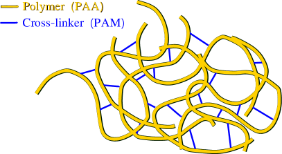
Figure 9: A schematic representation of short PAM oligomers (blue lines) forming bridges between PAA monomers (yellow lines).

Here the degree of cross linking is dictated by $\phi_{\rm PAM}$. The higher the $\phi_{\rm PAM}$ upto a threshold concentration, the larger the bridging connectivity and thus increased stiffness (as estimated from $K$) of materials. This increased $K$ then leads to elevated $\kappa$. Furthermore, the maximum value of $\kappa$ is observed around $\phi_{\rm PAM}\sim 0.3-0.4$. This is expected because when a small amount of PAM are blended in the PAA material, each PAM oligomer will bind to more than one PAA monomer to reduce the binding free energy [2, 43]. It should also be noted that the size of a PAM trimer is of the order of 0.75 nm, which is also typically equivalent to 2$-$3 times the PAA monomer size (see Figure 1). This length scale consistency also leads to almost perfect packing for PAA-PAM systems and thus forming three dimensional cross-linking networks. Moreover, when $\phi_{\rm PAM}$ is increased above a threshold value (for example $\phi_{\rm PAM}>0.4-0.5$) the effect is expected to be diluted because almost all PAA monomer will have at least one PAM to bind. Therefore, $\kappa$ values will then be dominated by the pure phases of the individual polymers, see Figure 8(a).

Lastly we would also like to emphasize that even when PAA-PAP blends phase separate, leading to no noteceable change in $\kappa$ with varying $\phi_{\rm PAP}$ (see Figure 7), di-block copolymer architectures (consisting of PAA and PAP blocks) may lead to interesting lamellar mesophases [44, 45] and, therefore, providing another route towards the tunability of $\kappa$ in amorphous polymers. In this context, layered superlattices (or thermal band gap materials) have been shown to exhibit interesting thermal behavior because of their interfacial properties [46]. Here, however, it should also be noted that in lamellar phases of di-block copolymers, unlike superlattices, phonon interference may not be expected to give a dominant contribution because the phonon mean free path is vanishingly small in amorphous solids and polymers [15, 39].

IV Conclusions and outlook

In this work, we have used molecular dynamics simulations to study thermal transport of asymmetric smart polymer blends and its connection to underlying macromolecular morphologies. For this purpose, we investigate two experimentally relevant polymer blends. Our structural analysis suggests that$-$ while a system of PAA-PAP blends are at the onset of phase separation, a system of PAA and PAM is fairly well miscible with significant excess hydrogen bonded interaction between cross species. The short PAM chains act as cross-linking bridges between monomers of different PAA chains forming a three dimensional (hydrogen bonded) highly cross-linked smart polymer network, thus increasing materials stiffness and improved thermal transport coefficient $\kappa$. We want to emphasize that the absolute values of $\kappa$ calculated in our simulations are within the experimental uncertainty and also consistent with the stiffness measurements. A rather generic picture emerging of these results is that $\kappa$ may be tuned when a system satisfies a few key conditions: miscibility, preferential hydrogen bonding, and the formation of cross-linking networks. Although we have presented data for PAA-PAM systems with improved $\kappa$, our simulation results indicate a rather generic design principle for plastic materials with the improvement and tunability of $\kappa$. To validate the protocol presented in this work, more detailed experimental synthesis, characterization, and their thermal transport measurements are needed on a broader spectrum of polymeric materials. Moreover, results presented here may serve as a guiding principle for the operational understanding and functional design of advanced materials with tunable properties.

V Acknowledgement

D.M. thank Kurt Kremer and Carlos M. Marques for fruitful continual collaborations that lead to the understanding of smart polymers presented here. We thank Derek Fujimoto for useful discussions. We further acknowledge support from Compute Canada where simulations were performed.

References

- [1] Cohen-Stuart, M. A.; Huck, W. T. S.; Genzer, J.; Müller, M.; Ober, C.; Stamm, M.; Sukhorukov, G. B.; Szleifer, I.; Tsukruk, V. V.; Urban, M.; Winnik, F.; Zauscher, S.; Luzinov, I.; Minko, S. Emerging applications of stimuli-responsive polymer materials. Nat. Materials 2010, 9, 101.
- [2] Mukherji, D.; Marques, C. M.; Kremer, K. Polymer collapse in miscible good solvents is a generic phenomenon driven by preferential adsorption. Nat. Commun. 2014, 5, 4882.
- [3] de Beer, S.; Kutnyanszky, E.; Schön, P. M.; Vancso, G. J.; Müser, M. H. Solvent induced immiscibility of polymer brushes eliminates dissipation channels. Nat. Commun. 2014, 5, 3781.
- [4] Halperin, A.; Kröger, M.; Winnik, F. M.; Poly(N-isopropylacrylamide) Phase Diagrams: Fifty Years of Research. Angew. Chem. Int. Ed. 2015, 54, 15342.
- [5] Zhang, Q; R. Hoogenboom, R. Polymers with upper critical solution temperature behavior in alcohol/water solvent mixtures. Prog. Pol. Science 2015, 48, 122.
- [6] Mukherji, D.; Marques, C. M.; Stuehn, T.; Kremer, K. Depleted depletion drives polymer swelling in poor solvent mixtures. Nat. Commun. 2017, 8, 1374.
- [7] Choy, C. L.; Thermal Conductivity of Polymers. Polymer 1977, 18, 984.
- [8] Shen, S.; Henry, A.; Tong, J.; Zheng, R.; Chen, G. Polyethylene nanofibres with very high thermal conductivities. Nat. Nanotech. 2010, 5, 251.
- [9] Hsieh, W.; Losego, M. D.; Braun, P. V.; Shenogin, S.; Keblinski, P.; Cahill, D. G. Testing the minimum thermal conductivity model for amorphous polymers using high pressure. Phys. Rev. B 2011, 83, 174205.
- [10] Hu, L.; Desai, T.; Keblinski, P. Thermal transport in graphene-based nanocomposite. J App. Phys. 2011, 110, 033517.
- [11] Pereira, L. F. C.; Donadio, D. Divergence of the thermal conductivity in uniaxially strained graphene. Phys. Rev. B 2013, 87, 125424.
- [12] Kodama, T.; Ohnishi, M.; Park, W.; Shiga, T.; Park, J.; Shimada, T.;Shinohara, H.; Shiomi, J.; Goodson, K. E. Modulation of Thermal and Thermoelectric Transport in Individual Carbon Nanotubes by Fullerene Encapsulation. Nat. Mat. 2017, 16, 892.
- [13] Mahoney, C.; Hui, C. M.; Majumdar, S.; Wang, Z.; Malen, J. A.; Tchoul, M. N.; Matyjaszewski, K.; Bockstaller, M. R. Enhancing thermal transport in nanocomposites by polymer-graft modification of particle fillers. Polymer 2016, 93, 72.
- [14] Kim, G.; Lee, D.; Shanker, A.; Shao, L.; Kwon, M. S.; Gidley, D.; Kim, J.; Pipe, K. P. High thermal conductivity in amorphous polymer blends by engineered interchain interactions. Nat. Mat. 2015, 14, 295.
- [15] Xie, X.; Li, D.; Tsai, T.; Liu, J.; Braun, P. V.; Cahill, D. G. Thermal Conductivity, Heat Capacity, and Elastic Constants of Water-Soluble Polymers and Polymer Blends. Macromolecules 2016, 49, 972.
- [16] Shanker, A.; Li, C.; Kim, G.; Gidley, D.; Pipe, K. P.; Kim, J. High thermal conductivity in electrostatically engineered amorphous polymers. Science Adv. 2017, 3, e1700342.
- [17] Tang, N.; Peng, Z.; Guo, R.; An, M.; Chen, X.; Li, X.; Yang, N.; Zang, J. Thermal Transport in Soft PAAm Hydrogels. Polymers 2017, 9, 688.
- [18] Xu, S.; Cai, S.; Liu, Z. Thermal Conductivity of Polyacrylamide Hydrogels at the Nanoscale. ACS App. Mat. Int. 2018, 10, 36352.
- [19] Li, C.; Ma, Y.; Tian, Z. Thermal Switching of Thermoresponsive Polymer Aqueous Solutions. ACS Mac. Letters 2018, 7, 53.
- [20] Wei, X.; Luo, T. The Role of Ionization in Thermal Transport of Solid Polyelectrolytes. arXiv:1904.01087.
- [21] Pronk, S.; Pall, S.; Schulz, R.; Larsson, P.; Bjelkmar, P.; Apostolov, R.; Shirts, M.R.; Smith, J.C.; Kasson, P.M.; van der Spoel, D.; Hess, B.; Lindahl, E. GROMACS 4.5: a high-throughput and highly parallel open source molecular simulation toolkit. Bioinformatics 2013, 29, 845.
- [22] Plimpton, S. Fast Parallel Algorithms for Short-Range Molecular Dynamics. J Comp. Phys. 1995, 117, 1.
- [23] Berendsen, H.J.C.; Postma, J.P.M.; van Gunsteren, W.F.; DiNola, A.; Haak, J.R. Molecular-Dynamics with Coupling to An External Bath. J. Chem. Phys. 1984, 81, 3684.
- [24] Essmann, U.; Perera, L.; Berkowitz, M.L.; Darden, T.; Lee, H.; Pedersen, L.G. A smooth particle mesh Ewald method. J. Chem. Phys. 1995, 103, 8577.
- [25] Hockney, R. W. The potential calculation and some applications. Methods Comput. Phys. 1970, 9, 135.
- [26] Hess, B.; Bekker, H.; Berendsen, H.J.C.; Fraaije, J.G.E.M. LINCS: A linear constraint solver for molecular simulations. J. Comp. Chem. 1997, 18, 1463 .
- [27] Jorgensen, W.L.; Maxwell, D.S.; Tirado-Rives, J. Development and Testing of the OPLS All-Atom Force Field on Conformational Energetics and Properties of Organic Liquids. J. Am. Chem. Soc. 1996, 118, 11225.
- [28] de Oliveira, T. E.; Mukherji, D.; Kremer, K.; Netz, P. A. Effects of stereochemistry and copolymerization on the LCST of PNIPAm. J Chem. Phys. 2017, 146, 034904.
- [29] Yuen H. K.; Tam E. P.; Bulock J. W. On the Glass Transition of Polyacrylamide. In: Johnson J.F., Gill P.S. (eds) Analytical Calorimetry. Springer, Boston, MA (1984).
- [30] Müller-Plathe, F. A simple nonequilibrium molecular dynamics method for calculating the thermal conductivity. J Chem. Phys. 1997, 106, 6082.
- [31] Zwanzig, R. Time-Correlation Functions and Transport Coefficients in Statistical Mechanics. Annu. Rev. Phys. Chem. 1965, 16, 67.
- [32] Torri, D.; Nakano, T.; Ohara, T. Contribution of inter- and intra-molecularenergy transfers to heat conduction in liquids. J Chem. Phys. 2008, 128, 044504.
- [33] Fan, Z.; Pereira, L. F. C.; Wang, H.; Zheng, J.; Donadio, D.; Harju, A. Force and heat current formulas for many-body potentials in molecular dynamics simulations with applications to thermal conductivity calculations. Phys. Rev. B 2015, 92, 094301.
- [34] Tschöp, W.; Kremer, K.; Batoulis, J.; Bürger, T.; Hahn, O. Simulation of polymer melts. I. Coarse-graining procedure for polycarbonates. Acta. Polym. 1998 49, 61.
- [35] Mukherji, D.; K. Kremer, K. Coil-globule-coil transition of PNIPAm in aqueous methanol: Coupling all-atom simulations to semi-grand canonical coarse-grained reservoir. Macromolecules 2013, 46, 9158.
- [36] Mukherji, D.; Wagner, M.; Watson, M. D.; Winzen, S.; de Oliveira, T. E.; Marques, C. M.; Kremer, K. Relating side chain organization of PNIPAm with its conformation in aqueous methanol. Soft Matter 2016, 12, 7995.
- [37] Binder, K.; Stauffer, D. Theory for the Slowing Down of the Relaxation and Spinodal Decomposition of Binary Mixtures. Phys. Rev. Lett 1974, 33, 1006.
- [38] Einstein, A. Elementare Betrachtungen über die thermische Molekularbewegung in festen Körpern 1911. Ann. Phys. 35:679.
- [39] Cahill, D. G.; Watson, S. K.; Pohl, R. O. Lower limit to the thermal conductivity of disordered crystals. Phys. Rev. B 1993, 46, 6131.
- [40] Braun, J. L.; Rost, C. M.; Lim, M.; Giri, A.; Olson, D. H.; Kotsonis, G. N.; Stan, G.; Brenner, D. W.; Maria, J.-P.; Hopkins, P. E. Adv. Mat. 2018, 30, 1805004.
- [41] Wang, W. H.; Wen, P.; Zhao, D. Q.; Wang, R. J. Relationship between glass transition temperature and Debye temperature in bulk metallic glasses. J. Mater. Res. 2003, 18, 2747.
- [42] Ashcroft, N. W.; Mermin, N. D. Solid state physics. Thompson Learning Inc. 2nd Edition 2004.
- [43] Mukherji, D.; Kremer, K. How does a poly(N-isopropylacrylamide) trigger phase separation in aqueous alcohol? Pol. Sci. Ser. C 2017, 59, 119.
- [44] Leibler, L. Theory of Microphase Separation in Block Copolymers. Macromolecules 1980, 13, 1602.
- [45] Fraser, B.; Dennistona, C.; Müser, M. H. On the orientation of lamellar block copolymer phases under shear. J. Chem. Phys 2006, 124, 104902.
- [46] Maldovan, M. Phonon wave interference and thermal bandgap materials. Nature Mat. 2015, 14, 667.