Classifying galaxies according to their Hi content

Abstract

We use machine learning to classify galaxies according to their Hi content, based on both their optical photometry and environmental properties. The data used for our analyses are the outputs in the range $z=0-1$ from Mufasa cosmological hydrodynamic simulation. In our previous paper, where we predicted the galaxy Hi content using the same input features, Hi rich galaxies were only selected for the training. In order for the predictions on real observation data to be more accurate, the classifiers built in this study will first establish if a galaxy is Hi rich ($\rm{log(M_{{\sc Hi}}/M_{*})}>-2$) before estimating its neutral hydrogen content using the regressors developed in the first paper. We resort to various machine learning algorithms and assess their performance with some metrics such as accuracy, $f_{1}$, ROC AUC, precision, specificity and log loss. The performance of the classifiers, as opposed to that of the regressors in previous paper, gets better with increasing redshift and reaches their peak performance around $z=1$ then starts to decline at even higher $z$. Random Forest method, the most robust among the classifiers when considering only the mock data for both training and test in this study, reaches an accuracy above $98.6\%$ at $z=0$ and above $99.0\%$ at $z=1$, which translates to a ROC AUC above $99.88\%$ at low redshift and above $99.96\%$ at higher one. We test our algorithms, trained with simulation data, on classification of the galaxies in RESOLVE, ALFALFA and GASS surveys. Interestingly, SVM algorithm, the best classifier for the tests, achieves a precision, the relevant metric for the tests, above $87.60\%$ and a specificity above $71.4\%$ with all the tests, indicating that the classifier is capable of learning from the simulated data to classify Hi rich/Hi poor galaxies from the real observation data. With the advent of large Hi 21 cm surveys such as the SKA, this set of classifiers, together with the regressors developed in the first paper, will be part of a pipeline, a very useful tool, which is aimed at predicting Hi content of galaxies.

1 Introduction

Much effort has been put into understanding the role of neutral hydrogen in galaxy formation and evolution. In the canonical picture based on the Hubble Sequence, the spiral galaxies are rich in cold gas and star forming, whereas the ellipticals are red and quiescent. However, an increasing number of observational evidence shows that these correlations are not always true. Local early-type galaxies from the ATLAS^3D survey were shown to contain significant cold gaseous components (Davis et al., 2011). They found that the relative angles between the gaseous and stellar planes show a bimodal distribution, but found no plausible explanation for such difference. This indicates that the gas distribution of a galaxy does not necessarily follow that of the stellar component. Therefore, direct inference of the gas content of galaxy based on its optical content is inaccurate. Elliptical galaxies are observed to form stars in cool core massive clusters (Donahue et al., 2011) that is suggestive of the presence of cold gas in those objects. The amount of gas components in massive ellipticals is crucial to understanding the evolution and growth of galaxies at the massive end, but the presence of kinematic abnormalities in their gas content as well as the uncertain effects of the Active Galactic Nuclei (AGN) feedback can affect the surface density of the gas content to pull the galaxies below the Hi detection limit, especially at higher redshifts.

Spiral galaxies are gas rich, but the limitations of observing the neutral gas at intermediate redshift prevent a robust study of the evolution of their gas content. Low redshift ($z\lesssim 0.4$) Hi can be observed with the 21cm emission line to provide the neutral hydrogen mass distribution of nearby galaxies. For instance, the Arecibo Legacy Fast ALFA (ALFALFA; Haynes et al., 2018) observed $\sim 30000$ galaxy Hi fluxes. The highest redshift galaxy ($z=0.376$) detected in 21 cm emission was observed with the COSMOS Hi Large Extragalactic Survey (CHILES) (Fernández et al., 2016). At any substantially higher redshift, the Hi content of galaxies is inferred from Damped Lyman Alpha systems (DLAs) in the spectra of background quasars, but it is difficult to measure the Hi mass from DLAs, and the relationship between galaxies and DLAs is not completely clear. The upcoming blind surveys such as Looking At the Distant Universe with the MeerKAT Array (LADUMA) on MeerKAT and eventually follow-up surveys on the SKA aim to measure the Hi content of galaxies at intermediate redshifts, to $z\sim 1$ and beyond.

The gas content of satellite galaxies are substantially impacted by environmental effects. Observationally, only $25\%$ of $\alpha.40$ (ALFALFA 40%; Haynes et al., 2011) galaxies were found to be in groups or clusters (Hess & Wilcots, 2013), which is lower than for the overall galaxy population. They found that in contrast to increasing optical sources towards to the center of groups or clusters, the number of Hi sources decreases. This is also supported from theoretical views. Using hydrodynamical simulation, Rafieferantsoa et al. (2015) showed that the fraction of Hi deficient galaxies increases towards higher halo masses. This is related to the star formation quenching timescale decrease towards higher halo mass: from $>3$ Gyr for $\mathrm{M_{halo}}<10^{12}\;{\rm M}_{\odot}$ to $<1$ Gyr for $\mathrm{M_{halo}}>10^{13}\;{\rm M}_{\odot}$ (Rafieferantsoa et al., 2019). Recent observational work by Foltz et al. (2018) agrees with this prediction, but in contrast Fossati et al. (2017) argues for no relationship between galaxy quenching timescales and halo mass. Simulations also suggest that the presence of Hi is strongly correlated with star formation, even if the star formation is physically occurring in molecular gas (Davé et al., 2017). Therefore, the Hi content appears to have a complex relationship with respect to stellar mass, star formation rate, morphology, and environment. This makes it challenging to predict what the Hi content of any given galaxy will be without accounting for the full range of its properties.

In order to better design and interpret upcoming Hi surveys, it is useful to be able to estimate the expected Hi content of galaxies that will be observed based on their already-measured multi-wavelength properties. To do so, here we develop and employ galaxy classification tools using machine learning. Galaxy classification is a very useful approach as it can provide insights into the physical processes by which galaxies evolve over cosmic time. There exist different and complementary ways to classify galaxies depending on the availability of the data, for instance morphological classification or spectral classification. The Hubble Sequence focuses on morphological classification, while spectral classification via absorption and emission lines provides more information about the chemical composition and stellar populations of galaxies (Morgan & Mayall, 1957). Zaritsky et al. (1995) developed a $\chi^{2}$-fitting approach to identify the best linear combination of template spectra that matches the observed spectrum in order to classify galaxies spectroscopically with low signal to noise ratio (S/N), and found good correlations of $\geq 80\%$ between spectra and morphology from Hubble classification. Slonim et al. (2001) presented a novel information bottleneck (IB) approach, improving on the then-standard geometrical and statistical approaches, to classify galaxy spectra using 2dF Galaxy Survey (Colless et al., 1998; Folkes et al., 1999). In a seminal work, Fukugita et al. (2007) conducted morphological classification of galaxies which was achieved by simple visual inspection where volunteers catalogued thousands of objects from Sloan Digital Sky Survey Data Release 3 (SDSS DR3; York et al., 2000) in order to obtain the rate of interacting galaxies. The need for automated classification arose with the increasing amount of available survey data, and it was demonstrated by Naim et al. (1995) and Lahav et al. (1996) that accuracy achieved by a trained Artificial Neural Network in classifying galaxies is comparable to that of a human expert. In a morphological classification of high redshift galaxies that Huertas-Company et al. (2008) conducted using Support Vector Machines, they argued that at $z>1$ early type galaxies were underestimated in the classifications using sample from COSMOS HST/ACS (Koekemoer et al., 2007) owing to the effects of morphological k-correction. In galaxy morphological classification, tree-based algorithms have also proved to be relatively robust classifier compared to other machine learning algorithms, as reported by Gauci et al. (2010). Hence there is a long history of using sophisticated galaxy classification methods in astronomy, but so far this has not been extensively applied to studying Hi.

In our previous work in Rafieferantsoa et al. (2018) (rad18 hereafter), we investigated the possibility of estimating the Hi content of galaxies using a variety of machine learning algorithms. Considering both the optical and environmental properties of the galaxies as input features, the algorithms were trained using large subsets of data from Mufasa simulation and tested on different subsets. They found that the performance of all regressors – assessed by using root mean squared error (rmse) and Pearson’s correlation coefficient (r) as metrics – degraded at higher redshift. Despite the tendency of all learners to under-predict the high Hi richness and over-predict the low one, random forest method – followed tightly by deep neural network – exhibited an overall best performance; achieving an rmse $\sim 0.25$ (corresponding to $\textbf{r}\sim 0.9$) at $z=0$. They then applied the regressors to real data from two different surveys, RESOLVE and ALFALFA. To this end, they trained the algorithms with an output from Mufasa at $z=0$ and used them to predict the Hi content of galaxies from real observations. Their results proved that the learners which they built can be potentially used for Hi study with the upcoming large Hi surveys like the SKA. Prior to this work, related study by Teimoorinia et al. (2017) also investigated the estimation of Hi content of galaxies based on the SDSS and ALFALFA data using 15 derived galaxy parameters.

However, in rad18 we only considered Hi rich galaxies ($\rm{log(M_{{\sc Hi}}/M_{*})}\geq-2$), hence the machine learning methods were trained to predict the gas content of Hi rich galaxies only. Therefore, at this stage, those algorithms on their own can’t be deployed in real world application where not all galaxies will be Hi rich. Models generally predict that galaxies are bimodal in their Hi content, particularly since satellite galaxies lose their Hi quite rapidly, after a delay period, once they enter another halo (Rafieferantsoa et al., 2019). To extend our work to be more generally applicable, we therefore need a way to classify galaxies as Hi rich or Hi poor based on available photometric data.

In this follow-up paper, we address this issue by building a set of learners that filter out the Hi poor galaxies in real survey, such that the regressors built in rad18 only predict galaxy gas content known to be above a certain threshold. Together with the classifiers, the regressors will form a pipeline which will be used to estimate Hi gas of galaxies in real observation. The approach is to use the same set of input features as in rad18 for the classification. This paper thus extends our approach to be more generally applicable to any galaxy survey that contains the requisite input features, which are chosen to be typically observationally accessible in present and upcoming multi-wavelength surveys.

We present our machine learning setup for our analyses in §2 and list all the algorithms we consider in §3. The results are shown in §4 and we demonstrate how the methods can be applied to data from real surveys in §5. We finally conclude in §6.

2 Setups

It is first noted that we make use of the same outputs ($z=0-1$) from Mufasa simulation to build our classifiers. Considering the Planck cosmological parameters $\Omega_{m}=0.3$, $\Omega_{\Lambda}=0.7$, $\Omega_{b}=0.048$, $H_{0}=68\;{\rm km}\,{\rm s}^{-1}\;{\rm Mpc}^{-1}$, $\sigma_{8}=0.82$ and $n_{s}=0.97$ (Planck et al., 2016), each snapshot results from simulating a comoving box of 50$h^{-1}$Mpc with a resolution of N = $512^{3}$ for each species (dark matter and gas). For the training, the features $\{u,g,r,i,z,U,V,J,H,K_{s},\Sigma_{3},v_{gal}\}$ are considered whereas our target – as in the case of a binary classification – is one of the two classes; 0 to denote Hi depleted galaxies ($\rm{log(M_{{\sc Hi}}/M_{*})}<v_{thresh}$) and 1 for Hi rich galaxies ($\rm{log(M_{{\sc Hi}}/M_{*})}\geq v_{thresh}$). To split the galaxies into two classes, one simply needs to run through all galaxies in the data and assign 0 or 1 to it if its gas content is below or above the threshold value v_thresh. In our case, we adopt v${}_{\mathrm{thresh}}=-2$, i.e. the Hi content is 2 orders of magnitude fewer than the stellar content.

Table 1: List of all the setups that are considered in the analysis. For easy reference, each setup has been given a name.

Name	Surveys	Features	Target	Description
fSMg	SDSS	$u,\>g,\>r,\>i,\>z,\>v_{gal},\>\Sigma_{3}$	$\rm log(M_{HI}/M_{*})$	redshift information not required
fSClr	SDSS	color indices,$\>v_{gal},\>\Sigma_{3}$	$\rm log(M_{HI}/M_{*})$	redshift information not required
fSCmb	SDSS	color indices, $u,\>g,\>r,\>i,\>z,\>v_{gal},\>\Sigma_{3}$	$\rm log(M_{HI}/M_{*})$	redshift information not required
fAMg	SDSS+Johnson+2MASS	$H,\>J,\>Ks,\>U,\>V,\>u,\>g,\>r,\>i,\>z,\>v_{gal},\>\Sigma_{3}$	$\rm log(M_{HI}/M_{*})$	redshift information not required
fAClr	SDSS+Johnson+2MASS	color indices,$\>v_{gal},\>\Sigma_{3}$	$\rm log(M_{HI}/M_{*})$	redshift information not required
zSMg	SDSS	$u,\>g,\>r,\>i,\>z,\>v_{gal},\>\Sigma_{3}$	$\rm log(M_{HI}/M_{*})$	prediction at a given redshift bin
zSClr	SDSS	color indices,$\>v_{gal},\>\Sigma_{3}$	$\rm log(M_{HI}/M_{*})$	prediction at a given redshift bin
zSCmb	SDSS	color indices, $u,\>g,\>r,\>i,\>z,\>v_{gal},\>\Sigma_{3}$	$\rm log(M_{HI}/M_{*})$	prediction at a given redshift bin
zAMg	SDSS+Johnson+2MASS	$H,\>J,\>Ks,\>U,\>V,\>u,\>r,\>r,\>i,\>z,\>v_{gal},\>\Sigma_{3}$	$\rm log(M_{HI}/M_{*})$	prediction at a given redshift bin
zAClr	SDSS+Johnson+2MASS	color indices,$\>v_{gal},\>\Sigma_{3}$	$\rm log(M_{HI}/M_{*})$	prediction at a given redshift bin

As in rad18, we adopt different setups both in terms of features and type of training which we present again in Table 1 for reference. For “$z-$training”, a classifier is built at each redshift bin whereas for “$f-$training” we make use of all data available in the range $z=0-0.5$. In contrast with the $f-$training in rad18, we do not go to higher $z$ to train the learner. In all cases, $75\%$ of the data is used for training and the remaining is used for testing.

3 Algorithms

We used a rather wide variety of machine learning algorithms in rad18 to see which one captures best the features from the data in order to make good predictions. Having gained a better understanding about how the methods dealt with information from the data, we consider most of them for this classification problem. It is worth reiterating that as opposed to regression task where the label is a numerical variable, the label for a classification task is a class – represented by integers mainly.

k-Nearest Neighbour (kNN) - Classification: the principle remains the same as in regression but instead of averaging the targets of $k-$closest neighbours to make prediction, the predicted class $y_{new}$ of a new instance $\textbf{x}_{new}$ is simply the majority of the classes of $k-$neighbours of $\textbf{x}_{new}$.

Random forest (RF) and Gradient boosting (GRAD) - Classification: decision tree is still the base estimator of both RF and GRAD. In contrast with its regressor counterpart, the decision tree classifier splits the training set at a split point $s_{i}$ using a feature $i$. The splitting is done in such a way as to minimize the objective function

$$\mathcal{F}=\frac{n_{R_{1}}}{n}G_{R_{1}}+\frac{n_{R_{2}}}{n}G_{R_{2}},$$ (1)

where $n_{R_{1}}$ is the number of examples in region $R_{1}$ and $n_{R_{2}}$ the number of examples in $R_{2}$. The total number of instances $n$ before the split is simply $n=n_{R_{1}}+n_{R_{2}}$. The Gini impurity $G$ of each region is given by

$$G=1-\sum_{i=1}^{k}p^{2}_{i},$$ (2)

where $p_{i}$ is the probability of an instance to belong to a class $i$ in the region. This can be computed by the ratio between the number of intances belonging to a class $i$ and the number of all instances in the region. The splitting can be done recursively on the resulting nodes depending on the required size of the tree. The RF method predicts the class of a new instance $\textbf{x}_{new}$ by aggregating the predictions of all its decision trees. The expression of the GRAD classifier is quite similar to Eq. 6 in rad18.

Deep neural network (DNN) - Classification: In contrast with the DNN regressor, the activation function of the output layer is a sigmoid function

$$\sigma(x)=\frac{1}{1+e^{-x}},$$ (3)

which computes the probabibility $p_{i}$ that an instance belongs to class $i$. In this case specifically, if $p\geq 0.5$, $y_{new}$ is 1 (positive class) whereas for $p<0.5$ $y_{new}$ is 0 (negative class). The objective function, known as log loss, is defined as

$$\mathcal{F}=-\frac{1}{N}\sum_{i=1}^{N}y_{i}{\rm{log}}(p_{i})+(1-y_{i}){\rm{log}}(1-p_{i}).$$ (4)

The weights and biases are updated via backpropagation as usual. The cost function in Eq. 4 can be generalised for multiclass case by using what is called cross entropy defined as

$$\mathcal{F}=-\frac{1}{N}\sum_{i=1}^{N}\sum_{k=1}^{\mathcal{K}}y_{k}^{i}{\rm{log}}(p_{k}^{i}),$$ (5)

where $\mathcal{K}$ is number of classes.

4 Galaxy classification

The objective in this work is to be able to establish whether a galaxy is Hi rich or Hi poor by exploiting both its optical and environmental data. To do so, we build various classifiers (see §3) and compare their performance qualitatively using various metrics which we present now along with some useful terminology in machine learning.

Accuracy: In binary classification, it measures the ratio of the correct predictions on a test sample, i.e.

$$accuracy=\frac{TP+TN}{FN+FP+TP+TN},$$ (6)

where $TP$ and $TN$ are True Positive – number of instances that are correctly predicted by the classifier to belong to 1 – and True negative – number of instances that are correctly predicted by the classifier to belong to 0 – respectively. FN or False Negative denotes the number of instances that belong to 1 but are classified as 0 and FP or False Positive indicates the number of instances that belong to 0 but are predicted as 1. A confusion matrix, which is represented in Figure. 1, is $2\times 2$ matrix which summarizes the predictions of a classifier on a test set.

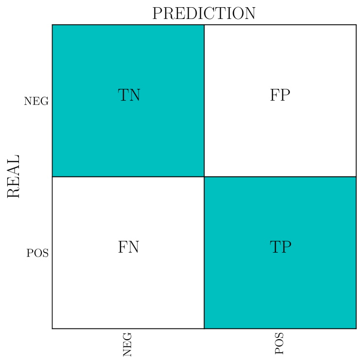
Figure 1: Confusion matrix $2\times 2$ for a binary classification. Negative class is Hi poor, Positive class is Hi rich.

Precision: It indicates how well the algorithm minimizes the number of instances incorrectly identified as a Positive class (FP) and is given by

$$precision=\frac{TP}{TP+FP}.$$ (7)

A good precision (high value close to one) translates to low FP.

Recall: Also called sensitivity, it characterizes the ability of the method to minimize the number of instances wrongly identified as a Negative class ($FN$). It is given by

$$recall=\frac{TP}{TP+FN}.$$ (8)

It is worth noting that, provided a classifier, if FP increases then FN decreases and vice versa. In other words, an increase in precision implies a decrease in recall – the so called precision-recall tradeoff. In our case, since we are mainly interested in identifying Hi rich galaxies whose gas content is to be predicted by our regressors built in rad18, we require our classifier to have good precision, as having a learner with a lower FP (hence higher it FN) – lower number of Hi poor galaxies predicted to belong to class of Hi rich galaxies – is in our case more preferable than a learner with a lower FN, hence higher FP.

$F_{1}$ score: This metric which combines $precision$ and $recall$ is their harmonic mean, given by

$$F_{1}=\frac{TP}{TP+\frac{FN+FP}{2}}.$$ (9)

High $F_{1}$ score simply means that both $precision$ and $recall$ are also high, which is the ideal case.

Log Loss: This quantity, given by Eq. 4, is also used as a metric. The lower its value, the better the classifier is.

Receiving Operating Characteristic - Area Under the Curve (ROC AUC): It is also possible to plot recall against FP rate which is given by $1-specificity$ where

$$specificity=\frac{TN}{TN+FP}.$$

As can be seen from Eqs.7-8, $FP$ follows the increase of recall as a consequence of the precision-recall trade-off. Another measure of the performance of a classifier is then to compute the area under the curve (recall vs FP rate). A perfect learner would have ROC AUC = 1.

A binary classifier uses a threshold parameter such that a new instance will be classified as positive or negative if the predicted probability is above or below the threshold respectively. A precision-recall (alternatively recall-FP rate) pair corresponds to a single value of a threshold parameter of a classifier and the idea behind the ROC curve is to find the best pair values precision-recall (alternatively recall-FP rate) in order to mitigate the trade-off between them, i.e. finding a threshold parameter value of the classifier such that both precision and recall are high. The results are now presented in the following.

4.1 Dependence on redshift

Table 1 lists the various setups that we feed to our machine learning algorithms. The name specifies whether it is uses $f-$training or $z-$training, whether we use SDSS data only (S) or all data including near-IR (A), and whether we use magnitudes (Mg) or colors (Clr) or combine them (Cmb). In all cases we use environment as measured by the third nearest neighbor ($\Sigma_{3}$), as well as the galaxy peculiar velocity ($v_{gal}$).

In Figure. 2, we show the results corresponding to each classifier selected in our investigation, considering only two metrics here, accuracy and $f_{1}$, for illustration purpose. The first column shows the accuracy achieved by each method with different input features for “$f-$training”, the second column is the resulting accuracy for “$z-$training”, the third column presents the $f_{1}$ score for “$f-$training” and finally the fourth one is the $f_{1}$ score for “$z-$training”.

Most classifiers attain accuracy and $f_{1}$ scores exceeding 0.9, which indicates that it is robustly possible to classify galaxies into Hi rich vs. Hi poor based on observable properties, at least in the idealised case of training and testing on simulated data alone. Still, there are clear differences among the classifiers. Random forests (RF; green) clearly exhibits the best performance whereas GRAD (purple) is relatively the weakest. For instance, RF (“$z-$training”) $accuracy$ and $f_{1}$ both reach $\sim 0.98$ at $z=0$ and $\sim 0.99$ at $z=1$, with similar values when combining data from $z=0-0.5$ (“$f-$training"). kNN shows values $\sim 0.95$, while DNN’s performance is consistently poorer.

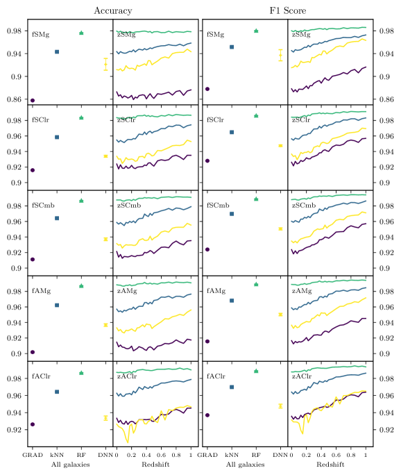
Figure 2: Accuracy and $f_{1}$ are shown on the 2 columns from the left and right, respectively. Good performance means high values of both accuracy and $f_{1}$. The dots, color coded by the training models we use, represent the performance (accuracy and $f_{1}$) of each classifier trained on all the data available between $z=0-0.5$, “$f-$training”. In the same way, the lines denote the value of the two metrics of each learner as a function of redshift “$z-$training”. Each row shows different results for different setups. The accuracy values are shown on the left y-axes and the $f_{1}$ values on the right y-axes.

The dependences of both accuracy and $f_{1}$ on redshift follow similar trend; they both increase as we go to higher $z$. This indeed looks very promising, since the improving performance of the classifier with increasing $z$ may compensate for the decreasing performance of the regressor built in rad18 at higher $z$, although this is only valid up to $z\sim 1$ since the performance of the classifier reaches their peak around that redshift then starts to degrade. That limitation is the reason we only show the results up to $z\sim 1$. In other words, most of the Hi poor galaxies can be filtered out by the classifier such that the regressor will only estimate the gas content of the Hi rich galaxies.

As expected, the value of the accuracy and that of $f_{1}$ when training the learners with all the data available between $z=0-0.5$ is approximately the average of accuracy’s and that of $f_{1}$’s within that $z$-bin. As already mentioned in rad18  the main idea behind the “$f-$training” is to anticipate the fact that in real observations, retrieving redshift information is not an easy task. Therefore we make an attempt at also building a classifier without relying on redshift information. The high values of both accuracy and $f_{1}$ $\sim 0.9$ for all learners with any setup except fSMg demonstrate that it is indeed possible to build a relatively good classifier without taking into account redshift information.

4.2 Dependence on input features

We now look in more detail at how the classification is affected by the selected input features, i.e. comparing the rows in Figure. 2. In realistic scenarios, it is not always possible to have all the features available. This leads us to investigate different scenarios by considering different combinations of features. The best classifier (RF) does appear to be insensitive to the choice of input features with values of accuracy and $f_{1}$ $\geq 0.98$ at all redshift bins, which is good news. However, for the learner with the worst performance (GRAD), it does not seem to be the case as its performance measures fluctuate with respect to the setup considered and are at their lowest values with zSMg setup (at $z=0$, $f_{1}$ and accuracy are both $\sim 0.87$; $z=1$, $f_{1}$ $\sim 0.91$ and $accuracy\sim 0.88$) for “$z-$training” and $accuracy\sim 0.857$ and $f_{1}$ $\sim 0.877$ for “$f-$training” fSMg.

In Figure. 3, we show other metrics of the RF, namely ROC AUC and log loss, as function of redshift for zSCmb. As expected, the better performance at higher redshift bin corresponds to a lower log loss. A ROC AUC $\geq 0.99$ at all redshifts corroborates the fact that RF is our best classifier for this ideal scenario where classifiers are both trained and tested with mock data.

It is noted that the effects of the class imbalance – potential issue owing to a big difference between the number of instances of each class in the training set which might cause a classifier to fail to label new instances in the test set properly – have been checked by compensating the imbalance using imblearn. No noticeable difference has been found between the two cases – with and without compensation – by comparing their resulting metrics.

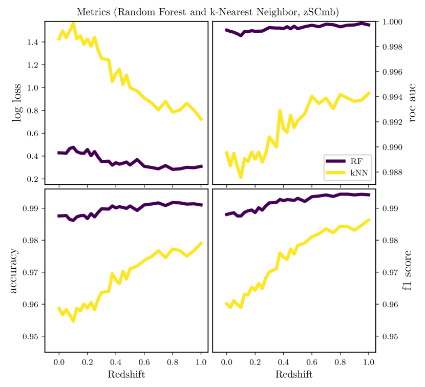
Figure 3: Four metrics as a function of $z$ of both RF and kNN methods for zSCmb setup. Top left: log loss, top right: ROC AUC, bottom left: accuracy and bottom right: $f_{1}$.

4.3 Effects of setting up the classes

In our main analyses, the Hi galaxies are split into two distinct classes according to whether their Hi gas masses are above or below a threshold of 0.01 times their stellar masses. The threshold value is broadly in accordance with observational Hi fraction limits. However, other classifications are possible. Here we explore the impact of changing the classification metric.

We consider three new classification schemes.

• The Galex Arecibo SDSS Survey (GASS; Catinella et al., 2013a) set a threshold limit of $\log(\mathrm{M_{HI}})=8.7$ for galaxies with $\mathrm{M_{*}}<10^{10.5}\;{\rm M}_{\odot}$ and $\log(\mathrm{M_{HI}/M_{*}})=-1.8$ otherwise. However, in order to be consistent with the threshold value of gas fraction used in rad18 to denote Hi depleted galaxies, we set it to be $\log(\mathrm{M_{HI}/M_{*}})=-2$. We call this type of splitting BIN.

• Another potential classification may be on whether a galaxy has higher Hi mass than stellar mass. In this case, the classes are given by $\Big{\{}\rm{log(M_{{\sc Hi}}/M_{*})}<0\rightarrow\textbf{0};\>\rm{log(M_{{\sc Hi}}/M_{*})}\geq 0\rightarrow\textbf{1}\Big{\}}$. We name this type of splitting LOW.

• Finally, we attempt splitting into three classes, as follows: $\Big{\{}\rm{log(M_{{\sc Hi}}/M_{*})}<-2\rightarrow\textbf{0};\>-2\leq\rm{log(M_{{\sc Hi}}/M_{*})}<0\rightarrow\textbf{1};\>\rm{log(M_{{\sc Hi}}/M_{*})}\geq 0\rightarrow\textbf{2}\Big{\}}$, which we call MULTI.

In Figure. 4, we compare the results corresponding to the RF method when considering three types of splitting, namely BIN (blue), LOW (orange) and MULTI (green). For brevity we only consider RF, since it is our best classifier, and $z-$training since the $f-$training values are expected to be similar.

Overall, both accuracy and $f_{1}$ are $\geq 0.80$ for all three types of splitting at all $z$ bins and it is quite clear that the algorithm performs best with our main type of splitting Hi poor/Hi rich, namely BIN. It is also interesting to see that the accuracy decreases with increasing redshift for both LOW and MULTI whereas $f_{1}$ increases as we go at higher redshift for LOW. Based on $accuracy$, the method performs similarly for LOW and MULTI splittings, but the difference in performance of the algorithm is striking when considering $f_{1}$ as a metric. This indicates that the classifier performance does depend on the classes chosen, but for our purposes of separating Hi rich and Hi poor galaxies, it performs very well even with minor changes to the scheme.

It is worth noting that in this idealised case and in the light of the results in rad18  we did not include SVM method. However, as will be shown later, we include it for the different tests on real observation data.

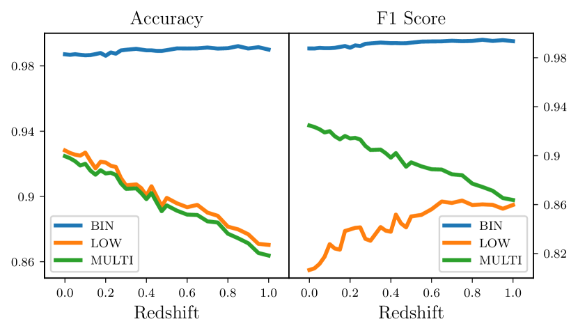
Figure 4: Left panel: accuracy as function of $z$, right panel: $f_{1}$ as a function of $z$. Blue is for BIN, orange for LOW and green for MULTI. The results are all related to RF algorithm.

5 Application to observational data

The lack of available data is one of the drawbacks of using machine learning when solving a problem, be it regression or classification. To mitigate that issue, in the context of Hi study, we aim at building classifiers trained with mock data from simulation and using them to identify Hi rich galaxies in real surveys.

As already demonstrated in rad18  the regressors that they built were able to learn from the mock data in order to predict the Hi content of the galaxies from both RESOLVE and ALFALFA. Our approach here is to redo the same exercise but for a classification task, i.e. training some classifiers with Mufasa data and utilising them to identify Hi rich galaxies from the same surveys, RESOLVE and ALFALFA. In this study, we also consider another survey, GASS, in which both Hi poor and Hi rich galaxies are better represented for our tests. For the description of the first two surveys, we refer the interested reader to rad18, and will now give a brief description of GASS.

5.1 GALEX Arecibo SDSS Survey (GASS) data

GASS was aimed at investigating Hi properties of a selected sample of galaxies ($\sim$ 1000) with available optical properties. The last data release (DR3) (Catinella et al., 2013b), which we use in our analyses, was built upon the first two data releases (Catinella et al., 2010, 2012). Within a relatively large volume survey of 200 Mpc already probed by SDSS primary spectroscopy survey, the GALEX Medium Imaging Survey and ALFALFA, galaxies have stellar masses of $10<\rm{log}(M_{*}/\rm{M_{\odot}})<11.5$ that encompasses the transition mass. The targets have Hi richness above the detection limit of $0.015$ for $10.5<\rm{log}(M_{*}/\rm{M_{\odot}})$ and a fix Hi mass of $10^{8.7}\rm{M_{\odot}}$ for lower stellar masses. The targets are designed to fall within $0.025<z<0.05$.

Using the Arecibo radio telescope, Catinella et al. (2013b) compiled a sample which has a fairly good representation in which $62\%$ are referred to as detections and the remaining $38\%$ as non detections. The latter represent galaxies in which a relatively small gas mass fraction was observed hence required a longer integration time (but not more than 3h), whereas the former was found to have relatively large amount of gas mass fraction. For our analyses, we retrieved all the optical properties of each galaxy in the sample from SDSS database using their SDSS-ID. In order to have a more balanced test sample, we then split the sample into two classes: Hi poor galaxies (class 0) are those with $\rm{log}(M_{HI}/\rm{M_{*}})<-1.55$ and the remaining are Hi rich galaxies (class 0). With this type of splitting, we have $56.8\%$ of the sample Hi rich and the remaining Hi poor.

5.2 Testing the built classifiers

We consider four different tests according to both the survey and input features

• TEST 1: RESOLVE DATA, color indices from all the band magnitudes available; SDSS (u,g,r,i,z), 2MASS (J,H,K), GALEX (NUV) and UKIDSS (Y,H,K)

• TEST 2: RESOLVE DATA, color indices from only SDSS (u,g,r,i,z) photometric data.

• TEST 3: ALFALFA, color indices from only SDSS (u,g,r,i,z) photometric data.

• TEST 4: GASS data, color indices from only SDSS (u,g,r,i,z) photometric data.

In all cases we split the simulated data for training and the considered test set into two categories, Hi poor (class 0) and Hi rich (class 1). Our results are summarised in Table 2 and shown in Figure 5.

5.3 TEST 1

The training set is composed of the data of snapshot at $z=0$ from Mufasa since the galaxies to be classified in RESOLVE survey are all at present epoch. We make use of all the photometric data available in RESOLVE, i.e. $\{u,g,r,i,z,J,H,Ks,NUV\}$. We consider 5 metrics – accuracy, $f_{1}$, ROC AUC, precision and specificity. The results of the classification from the learners selected in this work are presented in Table 2 and similarly shown in Figure 5.

DNN has the highest accuracy amongst the algorithms followed by RF. This is reminiscent to the results found in the regression problem in rad18. Despite the weaker performance of DNN compared to RF when testing on the simulated data (see Figure 2), testing on observational data really show the power of the algorithm. Nonetheless, all algorithms agree within $<10\%$. Based on the $f_{1}$ score and precision the methods are all comparable as well. Interestingly, DNN’s ROC AUC = 0.589 is the worst among all the methods, just above that of a classifier with a random guess.

Judging by the values of the precision which are $\geq 0.95$ for all methods, they satisfy what we require; classifiers that minimise the number of Hi poor galaxies incorrectly classified as Hi rich (FP) or in other words with high precision. However, a specificity equal to zero implies that all the negative class instances in the data are incorrectly classified (FP), bearing in mind that only 2$\%$ of this test sample are Hi-poor galaxies. Along with its high precision, SVM exhibits the highest specificity = 0.714, indicating its robustness, hence the best choice among the algorithms for this test.

We finally note that although $\sim 98\%$ for the RESOLVE galaxies are Hi-rich, Mufasa sample contains a balanced proportion of $\sim 52\%$ positive class making the training robust against class imbalance effect. The most important thing is the training part which is achieved using a well balanced sample (50/50 poor-rich), therefore the algorithms are not biased toward any class. In Test 4 we will consider a testing set that is more balanced (albeit smaller), which allows us to test our algorithm more fully.

Table 2: Summary of the results when using the simulation trained methods to classify Hi galaxies in the three different test tests.

	Accuracy	$f_{1}$	ROC AUC	Precision	Specificity
TEST 1
RF	0.974	0.987	0.633	0.979	0.0
GRAD	0.962	0.980	0.788	0.979	0.0
$k$NN	0.897	0.945	0.742	0.987	0.428
DNN	0.979	0.989	0.589	0.980	0.0
SVM	0.734	0.844	0.721	0.991	0.714
TEST 2
RF	0.774	0.870	0.829	0.991	0.666
GRAD	0.597	0.741	0.822	0.998	0.952
$k$NN	0.710	0.827	0.738	0.990	0.666
DNN	0.834	0.909	0.747	0.983	0.286
SVM	0.742	0.849	0.781	0.993	0.761
TEST 3
RF	0.948	0.973	0.953	1.0	1.0
GRAD	0.881	0.937	0.970	1.0	1.0
$k$NN	0.882	0.937	0.900	1.0	1.0
DNN	0.854	0.921	0.435	1.0	0.0
SVM	0.848	0.917	0.893	1.0	1.0
TEST 4
RF	0.642	0.659	0.685	0.717	0.683
GRAD	0.624	0.631	0.682	0.713	0.700
$k$NN	0.550	0.348	0.618	0.985	0.995
DNN	0.732	0.761	0.666	0.767	0.418
SVM	0.717	0.702	0.809	0.876	0.891

5.4 TEST 2

For this second test, we still use the RESOLVE data but consider color indices formed out of SDSS photometric data only, i.e. $\{u,g,r,i,z\}$. In contrast with TEST 1, the results in Table. 2 (Figure 5) suggest that, with the selected inputs features, the methods are capable of better identifying the gas poor galaxies with specificity all above $0.5$, except for DNN with $0.286$. In terms of Accuracy and $f_{1}$ scores, DNN is remarkably better and GRAD noticeably worse compared to RF and $k$NN. Based on ROC AUC, RF and $k$NN score the best and worst respectively. Based on the value of its precision = 0.998, it is tempting to say that GRAD is the best method for this test, however the results suggest that SVM generalises better than GRAD, as indicated by its $f_{1}$ score and accuracy. It is quite surprising to notice that with the same data (training/test), decreasing the number of selected features provide better information to the algorithms such that they get better at classifying the instances properly i.e precision (TEST 2) > precision (TEST 1); specificity (TEST 2) > specificity (TEST 1).

5.5 TEST 3

In this test, we use ALFALFA data and only consider SDSS photometric data for the input features as in TEST 2. Overall, all the methods perform much better as suggested by the high values of the metrics considered (see Table. 2). We note that the training set is the same as the one used for RESOLVE, hence class imbalance is not an issue that requires to be alleviated during training. The precision and specificity which are both equal to 1 clearly imply that FP is zero, hence class 0 instances, despite their relatively low number, are all correctly classified. This applies to all classifiers with the exception of DNN which has a specificity = 0. The results for this test then suggest that our classifiers are capable of recognizing Hi rich and Hi poor galaxies to a very good precision. The $f_{1}$ scores (all $>0.9$) of all the learners show that their recall’s are optimised, which also means that FN (Hi rich galaxies that incorrectly classified as Hi poor) is minimised. The relatively higher average precision (ROC AUC) of all classifiers (> 0.9) can indeed be used as an indicator that on average both FP and FN are minimised, this is not the case for DNN. All the trained non-neural network algorithms appear to meet our requirements but for the sake of comparison, RF method seems to be the best in this test, with the highest accuracy and $f_{1}$ values despite its ROC AUC is only second best. Conversly with the RESOLVE data, the DNN is definitely not favoured in properly classifying Hi-poor and Hi-rich galaxies when tests are done with blind survey data such as ALFALFA.

5.6 TEST 4

We use GASS data (Catinella et al., 2013b) for this test, considering SDSS photometric data as input features. Unlike the other samples used for testing so far, all classes (0, 1) are well represented in this dataset, with $56\%$ of this test set are Hi rich. Although kNN exhibits the highest precision and specificity, it does not generalise well, given its relatively low values of both accuracy and $f_{1}$. Results suggest that our best classifier for this test is SVM which has a relatively high precision (second best after kNN) and its tendency to generalise well as justified by its overall scores. In general, the other classifiers (RF, GRAD and DNN) are also capable of learning the features from the mock data in order to classify the real data, however the neural network model classifies poorly the Hi poor galaxies (i.e. low specifity values), as can be noticed in all the tests conducted.

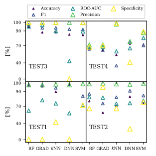
Figure 5: Summary of the results when using the simulation trained methods to classify the Hi content of galaxies from three different test sets from observational data. The y-axes are in exponential scale to prevent for data point cluttering.

6 Discussion and Conclusion

We have demonstrated in this work that it is possible to classify Hi galaxies based on their gas content using both their photometric and environmental data. We have built various algorithms by training them using large subset of the mock data ($75\%$) from Mufasa simulation. While being sensitive to:

• the inputs features,

• type of training (f-training or z-training),

• type of class splitting.

the test results, using smaller subset of Mufasa mock data (different from the subset on which they have been trained), look very promising. For instance, both Accuracy and $f_{1}$ score $>0.9$.

We have shown the good performance of the built classifiers when being tested on real observation data – RESOLVE, ALFALFA and GASS surveys – after training them on the mock data from Mufasa . Our findings can be summarized as follows:

• On using Mufasa to both train and test the learners, RF shows the best performance amongst the learners with an Accuracy of $99.00\%$ ROC AUC above $99.96\%$, $f_{1}$ score   $99.4\%$ at $z=1$. Other classifiers like k-NN and DNN also perform similarly well in general, however GRAD method shows poor performance when considering zSMg and fSMg setups.

• For z- training, Accuracy and $f_{1}$ score increase from present to higher redshift. The increase is steeper at $z<0.5$ and flattens out at higher redshift. This indeed compensates the fact that regressors built in rad18 perform best at low redshift and more poorly with increasing $z$.

• The performances of the regressors appear to be insensitive to the selected input features for the training except with the case of GRAD method which struggles to properly classify the galaxies in the test set when only considering SDSS magnitudes and environmental information as input features (zSMg and fSMg).

• The results are affected by the definition of the class of galaxies(BIN, LOW and MULTI). BIN, which is the type of splitting behind the motivation for this work, corresponds to better results compared to the other two types of splittings.

• Comparing the results corresponding to four different tests using real observational data from RESOLVE, ALFALFA and GASS surveys, with the exception of DNN as suggested by its low value of ROC AUC and zero specificity, the classifiers perform best on TEST 3 in which the test set is ALFALFA data and the input features considered are color indices formed out of SDSS magnitudes only. All learners correctly classified the Hi poor galaxies with a specificity = 1.0 and their precision is also maximised (precision = 1.0), which is what we really aim for. For TEST 3, it is quite clear that most of the errors (if not all) come from FN, i.e. Hi rich galaxies misclassified as Hi poor, although this quantity is already minimised given the rather high $f_{1}$ score of all the learners. By comparing TEST 1 and 2, it is clear that using color indices from SDSS data only is the optimal option to better identify the Hi poor galaxies given the higher precision in TEST 2. DNN has the highest Accuracy and $f_{1}$ for TEST 1 and TEST 2, indicative of being robust in classifying the Hi-rich galaxies. However, DNN fails to achieve a resonable classification of the Hi-poor galaxies as shown by the low values of Specificity ($<0.3$) for all tests. The relatively poor performance of DNN quantified by the slightly lower values of Accuracy and $f_{1}$ for TEST 3 compared to TEST 1 and TEST 2 might be due to the nature of the test samples. We speculate that the neural network is able to achieve higher performance in a cleaner set of data such as from the RESOLVE survey but under-perform in a sample from blind survey data such as ALFALFA. This does not mean the learner itself is not performing well, it only means that the data to test on are prone to higher systematic errors.

• In TEST 4 we use a test sample from GASS, which unlike the other samples used in the first three tests, has a fairly good representation of the two classes (i.e.Hi rich-Hi poor). This makes it a good dataset for assessing how well the classifiers are able to apply the learned features from the mock data. Based on the most important performance metric in this study, k-NN is the best classifier for TEST 4 with a precision = 0.985. It also classifies the Hi poor galaxies properly as demonstrated by its high specificity (0.995). However, even though our purpose is to build a classifier that has a very good precision which translates to its ability to correctly classify Hi rich galaxies, in all kinds of machine learning tasks, the algorithm that can minimise the generalisation errors well is the more preferable. In this case specifically, as the results suggest, SVM proves to be able to generalise well as shown by its accuracy (0.717), $f_{1}$ score (0.702), ROC AUC (0.809) and both precision and specificity are the second best.

• Overall in terms of performance, based on the scores in all tests on real data, we find that SVM is the best classifier as it demonstrates quite well its generalisation ability, learning from simulated data in order to classify real data.

With the advent of large Hi surveys like LADUMA and MIGHTEE, we have presented the possibility of properly classifying galaxies according to their gas content, using machine learning. The robustness of our methods lie in the fact that the trained algorithms can learn from mock data in order to classify galaxies in real surveys, which is indeed a strong asset in the sense that in reality the lack of enough data to train the methods turns out to be an issue that requires to be mitigated. Together with the regressors built in rad18, the classifiers in this work will form a useful pipeline to create mock Hi surveys for assisting with survey design, and eventually, will enable more detailed tests of the input model by comparing observed Hi to that predicted from the regressor on a case-by-case basis.

We only analysed the performance of single models in both this work and rad18. However, the use of more complex models using ensemble or stacking techniques are increasingly favoured in the literatures. We will explore such methods in future work despite their level of complexity as well as their interpretability.

References

- Catinella et al. (2010) Catinella B., et al., 2010, Monthly Notices of the Royal Astronomical Society, 403, 683
- Catinella et al. (2012) Catinella B., et al., 2012, Astronomy & Astrophysics, 544, A65
- Catinella et al. (2013a) Catinella B., et al., 2013a, MNRAS, 436, 34
- Catinella et al. (2013b) Catinella B., et al., 2013b, Monthly Notices of the Royal Astronomical Society, 436, 34
- Colless et al. (1998) Colless M., Morganti R., Couch W., 1998, in eds Morganti R. & Couch WJ, ESO/Australia Workshop, Springer, Pg.
- Davé et al. (2017) Davé R., Rafieferantsoa M. H., Thompson R. J., Hopkins P. F., 2017, MNRAS, 467, 115
- Davis et al. (2011) Davis T. A., et al., 2011, MNRAS, 417, 882
- Donahue et al. (2011) Donahue M., de Messières G. E., O’Connell R. W., Voit G. M., Hoffer A., McNamara B. R., Nulsen P. E. J., 2011, ApJ, 732, 40
- Fernández et al. (2016) Fernández X., et al., 2016, ApJ, 824, L1
- Folkes et al. (1999) Folkes S., et al., 1999, Monthly Notices of the Royal Astronomical Society, 308, 459
- Foltz et al. (2018) Foltz R., et al., 2018, preprint, (arXiv:1803.03305)
- Fossati et al. (2017) Fossati M., et al., 2017, ApJ, 835, 153
- Fukugita et al. (2007) Fukugita M., et al., 2007, The Astronomical Journal, 134, 579
- Gauci et al. (2010) Gauci A., Adami K. Z., Abela J., 2010, arXiv preprint arXiv:1005.0390
- Haynes et al. (2011) Haynes M. P., et al., 2011, AJ, 142, 170
- Haynes et al. (2018) Haynes M. P., et al., 2018, ApJ, 861, 49
- Hess & Wilcots (2013) Hess K. M., Wilcots E. M., 2013, AJ, 146, 124
- Huertas-Company et al. (2008) Huertas-Company M., Rouan D., Tasca L., Soucail G., Fevre O. L., 2008, Astron. Astrophys., 478, 971
- Koekemoer et al. (2007) Koekemoer A. M., et al., 2007, The Astrophysical Journal Supplement Series, 172, 196
- Lahav et al. (1996) Lahav O., Nairn A., Sodré L., Storrie-Lombardi M., 1996, Monthly Notices of the Royal Astronomical Society, 283, 207
- Morgan & Mayall (1957) Morgan W. W., Mayall N., 1957, Publications of the Astronomical Society of the Pacific, 69, 291
- Naim et al. (1995) Naim A., Lahav O., Sodre Jr L., Storrie-Lombardi M., 1995, Monthly Notices of the Royal Astronomical Society, 275, 567
- Planck et al. (2016) Planck et al., 2016, A&A, 594, A13
- Rafieferantsoa et al. (2015) Rafieferantsoa M., Davé R., Anglés-Alcázar D., Katz N., Kollmeier J. A., Oppenheimer B. D., 2015, MNRAS, 453, 3980
- Rafieferantsoa et al. (2018) Rafieferantsoa M., Andrianomena S., Davé R., 2018, Monthly Notices of the Royal Astronomical Society, 479, 4509
- Rafieferantsoa et al. (2019) Rafieferantsoa M., Davé R., Naab T., 2019, MNRAS, 486, 5184
- Slonim et al. (2001) Slonim N., Somerville R., Tishby N., Lahav O., 2001, Monthly Notices of the Royal Astronomical Society, 323, 270
- Teimoorinia et al. (2017) Teimoorinia H., Ellison S. L., Patton D. R., 2017, MNRAS, 464, 3796
- York et al. (2000) York D. G., et al., 2000, The Astronomical Journal, 120, 1579
- Zaritsky et al. (1995) Zaritsky D., Zabludoff A. I., Willick J. A., 1995, arXiv preprint astro-ph/9507044