X-Ray and Gamma-Ray Emission From Core-collapse Supernovae: Comparison of Three-dimensional Neutrino-driven Explosions With SN 1987A

Abstract

During the first few hundred days after the explosion, core-collapse supernovae (SNe) emit down-scattered X-rays and gamma-rays originating from radioactive line emissions, primarily from the ⁵⁶Ni $\rightarrow$ ⁵⁶Co $\rightarrow$ ⁵⁶Fe chain. We use SN models based on three-dimensional neutrino-driven explosion simulations of single stars and mergers to compute this emission and compare the predictions with observations of SN 1987A. A number of models are clearly excluded, showing that high-energy emission is a powerful way of discriminating between models. The best models are almost consistent with the observations, but differences that cannot be matched by a suitable choice of viewing angle are evident. Therefore, our self-consistent models suggest that neutrino-driven explosions are able to produce, in principle, sufficient mixing, although remaining discrepancies may require small changes to the progenitor structures. The soft X-ray cutoff is primarily determined by the metallicity of the progenitor envelope. The main effect of asymmetries is to vary the flux level by a factor of ${\sim}$3. For the more asymmetric models, the shapes of the light curves also change. In addition to the models of SN 1987A, we investigate two models of Type II-P SNe and one model of a stripped-envelope Type IIb SN. The Type II-P models have similar observables as the models of SN 1987A, but the stripped-envelope SN model is significantly more luminous and evolves faster. Finally, we make simple predictions for future observations of nearby SNe.

1 Introduction

A core-collapse supernova (CCSN) is the death of a massive star (Baade & Zwicky, 1934; Hoyle & Fowler, 1960), but the exact nature of the explosion remains obscured. The so-called delayed neutrino-heating mechanism (Colgate & White, 1966; Arnett, 1966; Bethe & Wilson, 1985; Bruenn, 1985) is a leading hypothesis in which a stalled shock is revived by neutrinos emitted from the surface of a hot proto-neutron star (for reviews, see Janka 2012, 2017; Burrows 2013; Müller 2016; Janka et al. 2016; Couch 2017). Recent three-dimensional (3D) simulations are able to include the basic physics necessary to describe the neutrino interaction and heating, and to simulate the outcome of the Fe core collapse, which then connects to the long-term simulations involving the whole star (Wongwathanarat et al., 2013, 2015, M. Gabler et al. 2019, in preparation). These simulations demonstrated that 3D effects are important both for the neutrino heating and the hydrodynamic instabilities above the Fe core.

To verify the supernova (SN) theory and assumptions that go into the simulations, it is important to compare the model predictions with observations. The spatial density and abundance distributions of the ejecta provide key information about the progenitor and explosion mechanism of CCSNe. Another valuable property that is observable is the X-ray and gamma-ray emission up to approximately 1000 days after the explosion (d). This emission arises from the radioactive decays of the unstable isotopes synthesized during the first few seconds after core collapse (Hoyle, 1954; Burbidge et al., 1957; Fowler & Hoyle, 1964; Hix & Harris, 2017). When an unstable isotope decays, gamma-rays are emitted. These gamma-rays lose energy due to Compton scattering as they propagate through the ejecta, and are then either destroyed by photoelectric absorption or escape the ejecta. An advantage of studying the early X-ray and gamma-ray emission is that the emission can be computed directly from the ejecta models without a need of specifying the microscopic mixing since the thermal conditions are decoupled from the high-energy radiation field (Jerkstrand et al., 2011). The emission is thus a sensitive probe of the macroscopic mixing and the ejecta structure. Additionally, the relevant physics for the photon propagation is well-known and the gamma-ray transfer is computationally cheap compared to more general radiation transfer (Hillier & Dessart, 2012; Jerkstrand et al., 2016).

Several groups have applied this method to compute the X-ray and gamma-ray emission from CCSN models. Previous studies of 3D models have explored bipolar Type II SN models (Hungerford et al., 2003) and single-lobe Type II explosion models (Hungerford et al., 2005). Maeda (2006) investigated jet-like broad-lined SN models and Wollaeger et al. (2017) computed both optical and high-energy spectra from a unimodal 3D model. A large number of models were also created and studied shortly after SN 1987A (catalog ) (for an overview, see McCray, 1993). This early modeling of SN 1987A was based on much more simplified 1D simulations. There are also several studies that have applied analogous methods to Type Ia SN (Burrows & The, 1990; Höflich, 2002; Sim, 2007; Sim & Mazzali, 2008; Kromer & Sim, 2009; Maeda et al., 2012; Summa et al., 2013; The & Burrows, 2014) and kilonova models (Hotokezaka et al., 2016; Korobkin et al., 2019).

In addition to the (down-scattered) X-rays and gamma-rays from the radioactive decay, other processes can also contribute to the high-energy emission. Lines from electron transitions are only relevant below 10 keV in SNe, which is at lower energies than the component from the radioactive decay. The photons from the radioactive decay also produce fast recoil electrons through Compton scattering. The bremsstrahlung emission from these electrons is expected to be much fainter than the emission from the radioactive decay in the relevant energy range (Clayton & The, 1991; Burrows & van Riper, 1995). Interactions with the circumstellar medium (CSM) is another potential source of X-rays (Chevalier & Fransson, 1994, 2017). This is a weak component for the vast majority of all SNe (Dwarkadas, 2014) and is typically at lower X-ray energies, although the hard X-ray regime is CSM-dominated in some cases. Examples of such cases include the nearby, strongly-interacting SN 1993J (Leising et al., 1994; Fransson et al., 1996) and the extremely luminous Type IIn SN 2010jl (Chevalier & Irwin, 2012; Ofek et al., 2014). Such CSM interaction results in spectra and light curves that are very different from those produced by reprocessed radioactive decay. Additionally, the gamma-ray continuum and, in particular, the direct line emission from the radioactive decay are unlikely to be confused with other emission components, even under extreme circumstances.

In this paper, we compute the early X-ray and gamma-ray emission from recent full 3D SN models based on neutrino-driven explosion simulations (Wongwathanarat et al., 2013, 2015) and compare the predicted emission properties to observations of SN 1987A. SN 1987A was a CCSN in the Large Magellanic Cloud (LMC), which makes it the closest observed SN in more than four centuries (for reviews, see Arnett et al. 1989; McCray 1993; McCray & Fransson 2016). The proximity of SN 1987A makes it the only CCSN where detailed observations of the early X-ray and gamma-ray evolution have been possible. The comparisons allow us to constrain properties of the ejecta structure and composition, and investigate the viability of recent SN simulations and SN 1987A progenitor models. We also investigate models of other types of SNe. This allows us to extend the results to more common SN types and serves as predictions for future observations.

This paper is organized as follows. We describe the SN models in Section 2 and the observations of SN 1987A in Section 3. The algorithm we use for the computations of the early emission is outlined in Section 4 and we present the results in Section 5. We discuss the results and important details in Section 6 and provide a summary and the main conclusions in Section 7.

2 Models

Table 1: Supernova Explosion Models

Model	Name	Type	$M_{\mathrm{ej}}$	$t_{\text{sim}}$	$E_{\mathrm{exp}}$	$Z_{\mathrm{eff}}$	$\langle v\rangle_{1\,\%}(^{56}\mathrm{Ni})$	$\langle M_{<}\rangle_{1\,\%}(^{56}\mathrm{Ni})$	Ref.
			(M☉)	(d)	($10^{51}$ erg)	(Zeff,☉)	(km s-1)	(M☉)
B15-1-pw	B15	BSG	14.2	156	1.43	0.55	3530	10.5	1, 2, 3, 4
N20-4-cw	N20	BSG	14.3	145	1.72	0.54	2110	14.8	3, 4, 5, 6, 7, 8
L15-1-cw	L15	RSG	13.7	146	1.71	0.30	4820	11.6	3, 4, 8, 9
W15-2-cw	W15	RSG	14.0	148	1.45	0.36	4190	11.5	3, 4, 8, 10
W15-2-cw-IIb	IIb	He core	13.7	118	1.52	0.36	6710	12.8	3, 4, 8, 10, 11
M157b-2-pw	M15-7b	Merger	19.5	111	1.43	0.47	3460	17.0	12, 13
M167b-2-pw	M16-7b	Merger	20.5	111	1.41	0.47	1770	16.7	12, 13

References. — (1) Woosley et al. (1988), (2) Bruenn (1993), (3) Wongwathanarat et al. (2015), (4) M. Gabler et al. (2019, in preparation), (5) Nomoto & Hashimoto (1988), (6) Saio et al. (1988), (7) Shigeyama & Nomoto (1990), (8) Wongwathanarat et al. (2013), (9) Limongi et al. (2000), (10) Woosley & Weaver (1995), (11) Wongwathanarat et al. (2017), (12) Menon & Heger (2017), (13) Menon et al. (2019)

We use SN models based on 3D neutrino-driven explosion simulations. An overview of the models is provided in Table 2. All progenitor models are 1D but are mapped into three dimensions with imposed low-amplitude random cell-by-cell perturbations to seed hydrodynamic instabilities for the SN explosion simulations (Wongwathanarat et al., 2013). Below, we describe the properties of the models that are most relevant to the current study. Comprehensive descriptions of all simulations can be found in the original references (Table 2).

All simulations included the neutrino luminosity as a free parameter, which effectively determines the final explosion energy ($E_{\mathrm{exp}}$). We note that we do not use the light-bulb approximation, meaning that the outgoing neutrino luminosities are considerably modified by the infalling material in our simulations. The neutrino luminosity was tuned to result in explosion energies of ${\sim}1.5\times{}10^{51}$ erg for all models. This roughly corresponds to estimates for SN 1987A (Woosley et al., 1988; Bethe, 1990; Bethe & Pizzochero, 1990; Shigeyama & Nomoto, 1990; Blinnikov et al., 2000; Utrobin, 2005), and is also fairly representative for ordinary Type II-P SNe (Kasen & Woosley, 2009; Pejcha & Prieto, 2015; Müller et al., 2017) and IIb SNe (Taddia et al., 2018).

For a given explosion energy, large variations are expected for the density and abundance distributions of the ejecta, which are determined by a coupled interaction between the explosion dynamics and progenitor structure (Wongwathanarat et al., 2015; Utrobin et al., 2019). In other words, these differences can be used to discriminate different progenitor models using observational data.

The M15-7b and M16-7b models are the results of mergers, whereas all the other models are single-star models. The B15, N20, M15-7b, and M16-7b models end their lives as blue supergiants (BSGs) and are designed to match the progenitor of SN 1987A. The B15 model is the single-star progenitor that yields the best agreement with the optical light curve of SN 1987A, based on self-consistent 3D explosion models (Utrobin et al., 2015). For the merger models, Menon et al. (2019) present results for artificially mixed 1D explosions while V. Utrobin et al. (2019, in preparation) present light curve analysis based on the 3D neutrino-driven explosion models.

We have investigated all six merger models of Menon & Heger (2017) that match the observational properties of the SN 1987A progenitor. We only present results from the M15-7b and M16-7b models here. The M15-7b model fits the X-ray and gamma-ray observations best and M16-7b is the worst model. This choice means that the X-ray and gamma-ray properties of M15-7b and M16-7b roughly bracket those of the complete set of merger models.

The L15 and W15 models are red supergiants (RSGs), which allow us to extend the results to Type II-P SNe, which is the most frequent type. Finally, model W15-2-cw-IIb (IIb) is an explosion of a nearly bare He core with a thin H envelope, which shows similarity to Cas A (Wongwathanarat et al., 2017).

All progenitors except the N20 and IIb models were created using self-consistent stellar evolution simulations. The N20 model (Shigeyama & Nomoto, 1990) was created by combining the core (Nomoto & Hashimoto, 1988) and envelope (Saio et al., 1988) of two different models. This was done in an attempt to match the properties of the progenitor of SN 1987A. The IIb model was created by artificially removing all but 0.3 M_☉ of the H envelope of Model W15-2-cw. This model is aimed to mimic a typical progenitor star of a Type IIb SN.

The mixing of ⁵⁶Ni is important for the early X-ray and gamma-ray emission. In Table 2, we provide the mass-weighted average radial velocity of the fastest 1 % of ⁵⁶Ni. This is similar to Wongwathanarat et al. (2015). Here, however, we weight the tracer element representing the uncertainty in the nucleosynthesis (referred to as X, Section 2.2) by 0.5 relative to ⁵⁶Ni, instead of 1.0, to remain consistent with the rest of this paper. The radial velocity of the fastest ⁵⁶Ni is a simplified representation of the amount of mixing in the models. The enclosed mass coordinate of the fastest ⁵⁶Ni should be related to the total ejecta mass ($M_{\mathrm{ej}}$) because of the importance of the amount of material outside of the fastest ⁵⁶Ni (Section 6.1).

The large range of fastest ⁵⁶Ni velocities indicates that the set of explosion models span a large range of mixing properties. The reason for this has been explored for the B15, N20, L15, and W15 models (Wongwathanarat et al., 2015; Utrobin et al., 2019). The mixing in these models is the result of a complex interplay between the progenitor structure, dynamics of the SN shock, and propagation of the neutrino-heated ejecta. One factor that favors efficient mixing is the fast growth of Rayleigh-Taylor instabilities at the (C+O)/He interface. Furthermore, a weak interaction of fast Rayleigh–Taylor plumes with the strong reverse shock occurring below the He/H composition interface also enhances the amount of mixing. So far, however, studies have relied solely on a small number of single-star progenitor models. Detailed analysis of the merger models and comparisons with single-star models will be presented in a future paper (V. Utrobin et al. 2019, in preparation).

Finally, we also include some comparisons with the 10HMM model (Pinto & Woosley, 1988) as a reference. It was fairly successful at describing several observables of SN 1987A and is representative of the extensive, but much more simplified, early work on the progenitor of SN 1987A (see Section 2.2 of McCray 1993). The 10HMM model is 1D and, importantly, has additional mixing introduced by hand.

2.1 Geometry

Of particular relevance to the gamma-ray transfer are the spatial resolutions of the simulations and the asymmetries caused by the hydrodynamic instabilities. The late-time simulations were run on axis-free Yin-Yang grids (Kageyama & Sato, 2004; Wongwathanarat et al., 2010) with a relative radial resolution better than 1 % at all radii and an angular resolution of 2°. For this study, the models are mapped from the Yin-Yang grids to spherical grids. The resolution of the spherical grids is sufficient to perform the mapping without significant loss of characteristic structures. The simulations provide no information on the small-scale mixing below the grid scale, but this does not affect the properties of the ejecta that are relevant for the gamma-ray propagation.

The H-rich single-star models are evolved until ${\sim}$150 d and the IIb model until 18 d, beyond which they can be assumed to expand homologously (M. Gabler et al. 2019, in preparation). The merger models are only available at an age of 1 d, from which we scale the models homologously. We check the effects of the late-time radioactive heating on the dynamics by comparing results from a version of the B15 model that has been expanded homologously from 1 d to the standard B15 model that has been followed by simulations until 156 d. The primary difference introduced by the late-time heating is increased mixing, leading to a flux increase of ${\sim}20$ % for most cases, although it can reach ${\sim}$40 % for the direct line emission at early times ($<200$ d). Homologous expansion is a reasonable approximation for a few thousand years (e.g., Truelove & McKee, 1999), but this period of the evolution could be more than an order of magnitude shorter in extreme cases, such as Type IIn SNe and in the presence of the equatorial ring in the case of SN 1987A. In general, the ejecta expand homologously inside of the reverse shock resulting from the interaction of the outermost ejecta with the CSM. During the first 1000 d of SN 1987A, before interaction with the equatorial ring, all of the ejecta can safely be assumed to expand homologously. In fact, the central parts of the ejecta that contain the majority of the mass are still freely expanding at current epochs (Fransson et al., 2013).

The explosion in all models sets in strongly asymmetrically as a consequence of hydrodynamic instabilities associated with the deposition of neutrino energy behind the stalled shock. This happens during the first seconds of post-bounce evolution. These initial explosion asymmetries trigger the growth of secondary non-radial hydrodynamic instabilities after the shock crosses the composition-shell interfaces on its way out from the center to the surface of the exploding star. A more detailed description of the ejecta asymmetries can be found in Section 5 of Wongwathanarat et al. (2015) and Section 3.3 of Utrobin et al. (2019).

2.2 Radioactive Elements

The nucleosynthesis is treated slightly differently in the different models. The nucleosynthesis in the SN 1987A models was followed by a network of elements that includes ¹H; the 13 $\alpha$-nuclei from ⁴He to ⁵⁶Ni; and a tracer nucleus X (Kifonidis et al., 2003; Wongwathanarat et al., 2013, 2015). The tracer represents elements that were produced in grid cells where the electron fraction was below 0.49. Therefore, X comprises neutron-rich, Fe-group elements, but the simulations provide no additional information about the compositions. The networks used for the RSG and IIb models omit ³²S, ³⁶Ar, ⁴⁸Cr, and ⁵²Fe.

Table 2: Nuclear Decay Data

Isotope	$\tau$	Ref.	Lines	Intensity	$E_{1}$	$I_{1}$	$E_{2}$	$I_{2}$
	(day)			($\gamma$ decay-1)	(keV)	($\gamma$ decay-1)	(keV)	($\gamma$ decay-1)
56Ni	$\hphantom{00}6.08$	1, 2, 3, 4	06	$3.21$	158	0.99	0812	0.86
56Co	$\hphantom{0}77.24$	1, 2, 3, 4	45	$2.91$	847	1.00	1238	0.68
57Co	$271.74$	1, 5, 6	10	$1.06$	122	0.86	0136	0.11

References. — (1) Firestone et al. (1999), (2) Junde (1992), (3) Junde (1999), (4) Junde et al. (2011), (5) Bhat (1992), (6) Bhat (1998)

The most important nuclear decay data are provided in Table 2.2. We follow the decays ⁵⁶Ni $\rightarrow$ ⁵⁶Co $\rightarrow$ ⁵⁶Fe (Clayton et al., 1969) and ⁵⁷Co $\rightarrow$ ⁵⁷Fe (Clayton, 1974). The most important transition during the relevant time intervals in the current context is ⁵⁶Co $\rightarrow$ ⁵⁶Fe. The transition ⁵⁷Co $\rightarrow$ ⁵⁷Fe dominates below 100 keV at epochs later than ${\sim}$800 d for the H-rich models and ${\sim}$300 d for the stripped IIb model. The contribution from the ⁴⁴Ti $\rightarrow$ ⁴⁴Sc $\rightarrow$ ⁴⁴Ca chain is negligible during the time periods considered in this paper. Finally, the isotope ⁵⁷Ni has a half-life of 36 h and is much less abundant than ⁵⁶Ni. The contribution of ⁵⁷Ni $\rightarrow$ ⁵⁷Co is, therefore, always negligible.

The true composition of X and the limited nuclear networks introduce uncertainties in the masses of individual isotopes. We compute the opacities based on the masses from the simulations, but rescale the escaping fluxes as if the masses of the radioactive sources match observations of SN 1987A for all models. All ⁵⁶Ni masses from the simulations are consistent, within the large uncertainties, with the ${\sim}$0.07 M_☉ of ⁵⁶Ni produced by SN 1987A (Suntzeff & Bouchet, 1990; Bouchet et al., 1991). The spatial distribution of ⁵⁶Ni is taken to be the distribution of the sum of the ⁵⁶Ni explicitly followed by the grid weighted by 1 and the tracer X weighted by 0.5. We investigate the effect of this choice by comparing results based on weighing the tracer by 0 and 1. The flux level varies by less than $25$ % in most cases, the shapes of the spectra are practically unchanged, and light curve peaks shift by less than ${\sim}$50 d.

We set the mass of ⁵⁷Ni by adopting a fixed ratio of the mass of ⁵⁷Ni relative to that of ⁵⁶Ni. The estimates of the ⁵⁷Ni$/$⁵⁶Ni ratio of SN 1987A from explosive nucleosynthesis networks (Thielemann et al., 1990; Woosley & Hoffman, 1991), direct observations (Syunyaev et al., 1990; Kurfess et al., 1992), and light curve modeling (Fransson & Kozma, 1993) favor values around twice the solar ratio, where the solar system ⁵⁷Fe$/\text{${}^{56}$Fe}$ number ratio is 0.023 (Lodders, 2003). The spatial distribution of ⁵⁷Ni is represented by the tracer X.

For consistency and for facilitating comparisons, we scale the fluxes of all models to match the radioactive isotope yields of SN 1987A. This puts the ⁵⁶Ni masses of our RSG explosions around the 80th percentile of the distribution of inferred yields of ordinary Type II-P SNe (Kasen & Woosley, 2009; Pejcha & Prieto, 2015; Müller et al., 2017; Anderson, 2019). In contrast, the ⁵⁶Ni mass of our IIb model is at the 20th percentile of the inferred ⁵⁶Ni masses of Type IIb SNe (Taddia et al., 2018; Anderson, 2019), which peaks at roughly twice the ⁵⁶Ni mass of SN 1987A.

2.3 Progenitor Metallicity

The progenitor metallicity is important because it determines the composition of the outermost parts of the models that are not mixed with the freshly synthesized material. The envelope metallicity significantly affects the emerging emission because the metals (primarily Fe) dominate the photoabsorption opacity in the relevant 10–100 keV range, even at metallicities that are much lower than the solar metallicity.

Instead of using the standard definition of metallicity, we define the effective metallicity ($Z_{\mathrm{eff}}$) as the photoabsorption opacity at 30 keV. This is done because the abundance patterns of the different models are different and the photoabsorption opacity is the most important consequence of the metallicity in the current context. The effective metallicities of all models are provided in Table 2. It is worth pointing out that the effective metallicity of the LMC is 0.54 Z_eff,☉. Relative to solar metallicity, this is slightly higher than what is typically adopted as the (standard) metallicity of the LMC. This is a result of Fe dominating the photoabsorption opacity above 6.4 keV and that Fe is not as under-abundant as many of the intermediate-mass elements.

Table 3: Adopted LMC Abundances

Element	LMC	Solar	Difference	LMC Ref.
	(dex)	(dex)	(dex)
H	$\equiv{}12$	$\equiv{}12$	$\cdots$	$\cdots$
He	10.93	10.90	$-$0.03	1, 2
C	17.81	18.39	$-$0.58	1, 2, 3, 4
O	18.35	18.69	$-$0.34	1, 2, 4, 5
Ne	17.58	17.87	$-$0.29	1, 2
Mg	17.06	17.55	$-$0.49	4, 5
Si	17.20	17.54	$-$0.34	4, 5
S	16.78	17.19	$-$0.41	1
Ar	16.48	16.55	$-$0.07	1
Ca	16.02	16.34	$-$0.32	1, 3
Ti	14.81	14.92	$-$0.11	6
Cr	15.42	15.65	$-$0.23	1, 3
Fe	17.23	17.47	$-$0.24	1, 3, 5

References. — (1) Table 12 of Russell & Dopita (1990), (2) Table 5 of Kurt & Dufour (1998); (3) Russell & Bessell (1989); (4) Table 17 of Hunter et al. (2007); (5) Table 9 of Trundle et al. (2007); (6) Table 1 of Russell & Dopita (1992)

Note. — The effective metallicity (see Section 2.3) of the LMC is $0.54$ Z_eff,☉. This is dominated by the difference in the Fe abundance of $-0.24$ dex. The solar abundances are included for reference.

The treatment of the metallicity in the stellar evolution simulations of the B15 and N20 progenitors has been significantly simplified. Those nuclear networks were reduced by omitting the heavier metals and representing the metallicity using only lighter elements. We correct for this by raising the mass fraction of each individual element to the LMC abundance in grid cells where the individual abundance is lower than the corresponding LMC value. Abundances are never lowered to match LMC abundances, which explains why the B15 model (0.55 Z_eff,☉) has marginally higher effective metallicity than the LMC (0.54 Z_eff,☉). We do not use abundances inferred from the equatorial ring of SN 1987A because this would require much larger changes to the models. See Section 6.1.3 for a discussion of using abundances inferred from the equatorial ring of SN 1987A instead of LMC abundances.

The adopted LMC abundances are provided in Table 2.3. The corrections are performed in regions where the H mass fraction is $>0.1$. The H mass fractions are slightly reduced to preserve the total masses. The total changes are approximately shifts of 0.1 M_☉ from H to metals, primarily intermediate-mass elements. We reiterate that only the B15 and N20 models require this modification. For example, the effective metallicity of the B15 model before correction is 0.03 Z_eff,☉. We also note that the RSGs, mergers, and IIb models are unmodified from their evolutionary compositions and have slightly lower effective metallicities (Table 2).

3 Observations of SN 1987A

We use early X-ray and gamma-ray observations of SN 1987A as an observational test of the simulated SN models. The comparisons can be divided into three categories; spectra, continuum light curves, and line fluxes. The observations of the line profiles are investigated in a separate paper (A. Jerkstrand et al. 2019, in preparation).

The distance to SN 1987A is taken to be 51.2 kpc (Panagia et al., 1991; Gould & Uza, 1998; Panagia, 1999; Mitchell et al., 2002) and when comparing simulations to observations, we correct the observed spectra for the recessional heliocentric velocity of the LMC of 287 km s^-1 (Gröningsson et al., 2008a, b). The ISM absorption is negligible in the relevant energy range of ${\sim}$10–3500 keV (e.g., Willingale et al. 2013; Frank et al. 2016).

Table 4: Early Hard X-Ray and Gamma-Ray Observations of SN 1987A

Instrument	Platform	Epoch	Energy Range	References
		(d)	(keV)
HEXE	Roentgen/Mir-Kvant	168–830	15–200	1, 2, 3, 4, 5, 6
Pulsar X-1	Roentgen/Mir-Kvant	168–830	70–600	1, 2, 3, 4, 5, 6
GRS	SMM	1–826	300–9000	7, 8, 9, 10
LAC	Ginga	2–1400	6–28	11, 12, 13, 14, 15
MSFC/Lockheed/Marshall	Balloon	95, 249, 411, 619	18–960	16, 17, 18, 19, 20
GRIP/Caltech/CIT	Balloon	86, 268, 414, 771	30–5000	21, 22, 23
GRIS/GSFC/Bell/SNLA/Sandia	Balloon	433, 613	20–8000	24, 25, 26, 27, 28
JPL	Balloon	286	50–8100	29
GRAD/Florida/GSFC	Balloon	319	700–3000	30
UCR Compton Telescope	Balloon	418	500–20,000	31, 32, 33

References. — (1) Sunyaev et al. (1987), (2) Syunyaev et al. (1987), (3) Syunyaev et al. (1988), (4) Syunyaev et al. (1989), (5) Syunyaev et al. (1990), (6) Sunyaev et al. (1991), (7) Forrest et al. (1980), (8) Matz et al. (1988), (9) Leising (1989), (10) Leising & Share (1990), (11) Makino & ASTRO-C Team (1987), (12) Dotani et al. (1987), (13) Tanaka (1988), (14) Tanaka (1991), (15) Inoue et al. (1991), (16) Sandie et al. (1988b), (17) Sandie et al. (1988a), (18) Wilson et al. (1988), (19) Fishman et al. (1990), (20) Pendleton et al. (1995), (21) Althouse et al. (1985), (22) Cook et al. (1988), (23) Palmer et al. (1993), (24) Teegarden et al. (1989), (25) Tueller et al. (1990), (26) Tueller et al. (1991), (27) Tueller (1991), (28) Barthelmy et al. (1991), (29) Mahoney et al. (1988), (30) Rester et al. (1989), (31) Zych et al. (1983), (32) Simone et al. (1985), (33) Ait-Ouamer et al. (1992)

An overview of all early hard X-ray and gamma-ray observations of SN 1987A is provided in Table 3. Some of the early X-ray and gamma-ray observations have also been summarized by other authors (Bunner, 1988; Gehrels et al., 1988; Leising, 1991; Teegarden, 1991; Tueller, 1991; Wamsteker, 1993). Below, we briefly describe the instruments and data used for our comparisons.

3.1 The Roentgen Observatory

The Roentgen Observatory was an experiment in the Kvant module of the space station Mir. The Kvant module carrying Roentgen docked to Mir during 1987 April and started observing SN 1987A 168 d after the outburst and continued to monitor SN 1987A to later than 800 d. We use data from the High Energy X-ray Experiment (HEXE) and the Pulsar X-1 instruments.

HEXE was the most sensitive instrument and provides relatively accurate continuum light curves in three energy bands in 15–200 keV (Syunyaev et al., 1990). Low-resolution spectra were also extracted for seven epochs. We also use spectra from Pulsar X-1 at 320 d (Syunyaev et al., 1988). The data are of significantly lower quality and are primarily included with the purpose of verifying the HEXE spectra above 70 keV during peak brightness, while also extending the energy coverage to 600 keV.

3.2 SMM

The Solar Maximum Mission (SMM) was launched in 1980 and was a dedicated solar observatory. One of the seven instruments on board was the Gamma-Ray Spectrometer (GRS), which operates in the energy range 0.3–8.5 MeV (Forrest et al., 1980). The moderate energy resolution of around 50 keV at 1 MeV is insufficient for resolving the radioactive line profiles. SMM was unable to point away from the Sun except for short durations, so SN 1987A was observed as a part of the background emission while SMM performed solar observations. Because SMM was operational for seven years before SN 1987A, it was possible to monitor the background gamma-ray flux before the explosion and then detect SN 1987A as a change in the background level during its early evolution.

We use data from SMM to constrain the evolution of the line fluxes. SMM provides the most accurate measurements of the line fluxes and also continuously monitored SN 1987A throughout its early evolution. No emission from SN 1987A was detected before 1987 July, but the ⁵⁶Co decay lines rose rapidly during 150 to 200 d (Matz et al., 1988). The line emission peaked shortly thereafter, and then decayed beyond the detection threshold around day 600 (Leising & Share, 1990).

3.3 Ginga

The X-ray astronomy satellite Ginga (“Galaxy”) was launched on 1987 February 5 and started observing SN 1987A two days after outburst and monitored SN 1987A for more than 1000 days. The first detection of emission from SN 1987A was on day 131 (Dotani et al., 1987). Ginga carried three instruments, but only data from the Large Area Proportional Counter (LAC) are used for this work. The LAC was a collimator and provided data on SN 1987A in the 6–28 keV range. Because of the relatively large collimator opening angle, the data might be contaminated by background sources (Inoue et al., 1991). For this reason, we choose to exclude data during an apparent flaring period in January 1988.

We use the Ginga light curves in the 6–16 and 16–28 keV ranges. For the presentations in this paper, we treat the two bands as spectral bins for the comparisons at specific times. The X-ray emission in the full 6–28 keV range consists of two emission components (Tanaka, 1988) and the energy cut at 16 keV was chosen to optimally separate them from each other (Inoue et al., 1991). The signal-to-noise ratio in the low-energy band is low and the emission could be the result of interactions with the CSM or bremsstrahlung from the fast recoil electrons. This means that the low-energy band is not strictly comparable to our predictions but could be viewed as an upper limit. The 16–28 keV component is less variable and most likely represents the low-energy cutoff of the Comptonized radioactive emission (Inoue et al., 1991; Tanaka, 1991). The Ginga data agree reasonably well with the Roentgen/HEXE data in the overlapping energy range.

3.4 Balloon-borne Experiments

We use data from a number of balloon-borne experiments, the details of which are summarized in Table 3. They provide independent measurements of the spectra (MSFC, GRIP), which agree well with the data from HEXE and Pulsar X-1. This effectively also verifies the continuum flux measurements of HEXE that are used to construct the continuum light curves. All of the balloon experiments that we include were able to measure line fluxes, which show reasonable agreement with the line flux evolution as observed by SMM (Figure 5 of Leising & Share 1990). Additionally, only balloon-borne experiments (GRIS, JPL, GRAD) carried instruments with sufficient energy resolution to resolve the line profiles of ⁵⁶Co (presented in A. Jerkstrand et al. 2019, in preparation).

4 Algorithm & Implementation

We compute the X-ray and gamma-ray properties by following the propagation of Monte Carlo (MC) photons through the ejecta. The interactions we include are photoelectric absorption, Compton scattering, and pair production. We do not compute bremsstrahlung or fluorescent emission because these effects only contribute significantly at energies below the sharp photoabsorption cutoff around 15 keV (Woosley et al., 1989; Clayton & The, 1991; Burrows & van Riper, 1995). We verify our code by comparing to previously published spectra and light curves (Milne et al., 2004; The & Burrows, 2014) of the W7 model (Nomoto et al., 1984), and by comparing results from our code to those from HEIMDALL (Maeda et al., 2014) and SUMO-3D (A. Jerkstrand et al. 2019, in preparation).

We use $\xi_{i}$ to denote random numbers uniformly distributed in the range 0 to 1, where the index $i$ distinguishes the different random numbers. Spatial vectors are denoted using boldface (e.g., $\boldsymbol{a}$), and the Cartesian components are $(a_{x},a_{y},a_{z})$. The spherical components are $(a_{\rho}{},a_{\phi}{},a_{\theta}{})$, where $\phi{}$ is the azimuthal angle ranging from 0 to $2\,\pi$, and the polar angle $\theta$ is defined from 0 at the north pole to $\pi$ at the south pole. Four-vectors are denoted using Greek indices (e.g., $b_{\mu}$). We denote quantities in the SN frame without primes and quantities in frames locally comoving with the homologous expansion with primes.

4.1 Cross Sections

In this section, we describe the cross sections used for Compton scattering, photoabsorption, and pair production. The absorption and scattering properties of the tracer X are set to those of ⁵⁶Fe.

4.1.1 Compton Scattering

The Compton scattering cross section is given by the Klein-Nishina formula (e.g., Rybicki & Lightman 1979). For computational stability and performance, we use an approximate expression for the Klein-Nishina cross section (p. 319 of Pozdnyakov et al., 1983). The difference between the approximation and the exact formula is less than 1 % at all energies.

The energy lost by a photon in each scattering in the rest frame of the electron is given by

$$\frac{E_{\mathrm{f}}^{\prime}}{E_{\mathrm{i}}^{\prime}}=\frac{1}{1+\frac{E_{\mathrm{i}}^{\prime}}{m_{\mathrm{e}}\,c^{2}}(1-\cos\alpha^{\prime})},$$ (1)

where $E_{\mathrm{f}}$ is the final photon energy, $E_{\mathrm{i}}$ the initial photon energy, $m_{\mathrm{e}}$ the electron mass, and $\alpha$ the scattering angle. It shows the important property that the fractional energy loss is much higher when the energy before scattering is comparable to, or higher than, the electron rest energy.

4.1.2 Photoelectric Absorption

Photoabsorption cross sections are quickly declining functions of energy $E$, which implies that photoabsorption is only relevant at relatively low X-ray energies. It starts becoming important around 100 keV and dominates below ${\sim}$40 keV for typical SN abundances (Alp et al., 2018). The non-relativistic high-energy asymptote is approximately proportional to $E^{-3}$. We use the cross sections of Verner et al. (1996).

We note that the cross sections of Verner et al. (1996) are very similar to those of Verner & Yakovlev (1995) at energies above 10 keV for the relevant isotopes, except for ⁴He. The photoabsorption cross section of ⁴He from Verner et al. (1996) is approximately 40 % lower than the value of Verner & Yakovlev (1995) but the effect on the escaping fluxes is only approximately 1 %. The cross sections of Verner et al. (1996) are also very similar to those of Veigele (1973).

4.1.3 Pair Production

We include pair production primarily for comparisons with other codes (Milne et al., 2004). We have indeed verified that this effect has a negligible impact on the results for the models studied in this paper. For example, for ⁵⁶Ni, the scattering cross section is 10 times higher than the pair production cross section at 3 MeV and they are approximately equal at 10 MeV (see Figure 1 of Milne et al., 2004). Typically, less than 0.1 % of the total photons are pair absorbed.

We take the pair production cross sections from Ambwani & Sutherland (1988), which interpolates tabulated values of the cross sections (Hubbell, 1969; Hubbell et al., 1980). The pair production cross sections are

$$\sigma_{\text{pp}}=\begin{cases}0\text{~{}cm}^{2}&E_{6}<1.022\text{~{}MeV}\\ 0.10063\,(E_{6}-1.022)\,Z^{2}\times 10^{-27}\text{~{}cm}^{2}&1.022\leq E_{6}<1.5\text{~{}MeV}\\ [0.0481+0.301\,(E_{6}-1.5)]\,Z^{2}\times 10^{-27}\text{~{}cm}^{2}&E_{6}\geq 1.5\text{~{}MeV}\end{cases},$$ (2)

where $E_{6}$ is the photon energy in units of MeV and $Z$ is the atomic number.

4.2 Photon Initialization

Gamma-ray photons are created by the decay of the radioactive isotopes in the inner regions of the ejecta. Each MC photon is initially created by assigning a spatial position $\boldsymbol{r}$, a direction of propagation $\boldsymbol{\Omega}$, and a photon energy. The initial spatial distribution is given by the spatial distribution of the parent nuclei in the models (Section 2.2). The direction of the photons are random in the rest frame of the homologously expanding parent nuclei, and the initial photon energies are the well-defined energies of the corresponding transitions. Important data about the radioactive lines included in the code are provided in Table 2.2. With the energy $E^{\prime}$ and the direction $\boldsymbol{\Omega^{\prime}}$, it is straightforward to construct the four-momentum $p_{\mu}^{\prime}$ and inverse Lorentz boost it to the SN frame. The result of accounting for the difference in reference frames is that the energies $E$ are Doppler shifted and $\boldsymbol{\Omega}$ slightly beamed in the outward direction. The effect on the result introduced by the beaming is an increase in escaping number flux of less than 1 %.

4.3 Photon Propagation

As the photon propagates through the ejecta, the optical depth is given by

$$\tau=\tau_{\mathrm{CS}}+\tau_{\mathrm{ph}}+\tau_{\mathrm{pp}},$$ (3)

where the scattering depth $\tau_{\mathrm{CS}}$, photoabsorption depth $\tau_{\mathrm{ph}}$, and pair production depth $\tau_{\mathrm{pp}}$ are given by

$$\tau_{\mathrm{CS}} =\int_{L}\!\sigma_{\mathrm{KN}}(\boldsymbol{r},E)\,n_{\mathrm{e}}(\boldsymbol{r})\,\mathrm{d}L$$ (4)

$$\tau_{\mathrm{ph}} =\int_{L}\!\sum_{I}\sigma_{\mathrm{ph}}(\boldsymbol{r},E,I)\,n(\boldsymbol{r},I)\,\mathrm{d}L$$ (5)

$$\tau_{\mathrm{pp}} =\int_{L}\!\sum_{I}\sigma_{\mathrm{pp}}(\boldsymbol{r},E,I)\,n(\boldsymbol{r},I)\,\mathrm{d}L,$$ (6)

where $L$ is the path traveled by the photon, $\sigma_{\mathrm{KN}}$ the Klein-Nishina cross section, $n_{\mathrm{e}}$ the electron number density, $\sigma_{\mathrm{ph}}$ photoabsorption cross section, $n$ the element number density, and the sums are taken over all elements $I$. The path is defined as the line starting from the position of the previous scattering, or the initial position if the photon has just been created. This integral is solved continuously as the photon travels through the ejecta by discretizing the continuous integral into a sum of finite $\mathrm{d}L$. The discretization is chosen such that the distance $\mathrm{d}L$ is equal to 1 % of the magnitude of the current radial position of the photon. It was verified that finer discretizations result in similar results and the spatial resolution is ultimately limited by the resolution of the models (see Section 2.1). A photon propagates until $\tau$ reaches a limiting optical depth $\tau_{\mathrm{lim}}$, which is sampled from the distribution

$$\tau_{\mathrm{lim}}=-\ln\xi_{\tau}.$$ (7)

At this point, one of the following three interactions occurs; the photon scatters off an electron, the photon is photoabsorbed, the photon pair produces.

4.4 Interactions

In this subsection, we describe how the different interactions are treated numerically at the point of interaction. Scattering affects the photon energy and the direction of propagation, but does not destroy the photon; photoabsorption destroys the photon; and pair production destroys the photon and creates an electron-positron pair. We assume that no positronium forms and that each positron is converted into a photon pair locally (Chugai et al., 1997; Ruiz-Lapuente & Spruit, 1998; Jerkstrand et al., 2011).

An interaction occurs when $\tau=\tau_{\mathrm{lim}}$. If the condition (Pozdnyakov et al., 1983)

$$\xi_{\mathrm{ph}}<\frac{\tau_{\mathrm{ph}}}{\tau_{\mathrm{cs}}+\tau_{\mathrm{ph}}+\tau_{\mathrm{pp}}}$$ (8)

is fulfilled, the photon is absorbed. Absorption means that the photon is destroyed and the program moves on by simulating the next MC photon. If Eq. (8) is not fulfilled, but

$$\xi_{\mathrm{ph}}<\frac{\tau_{\mathrm{ph}}+\tau_{\mathrm{pp}}}{\tau_{\mathrm{cs}}+\tau_{\mathrm{ph}}+\tau_{\mathrm{pp}}}$$ (9)

is fulfilled, the original photon is replaced by a pair of 511 keV photons with random directions in the locally comoving frame. This represents pair production and subsequent annihilation.

If neither condition is fulfilled, scattering occurs and a new direction and energy are computed. Both the new photon direction and energy are dependent on the velocity of the scattering electron. The electron velocities are taken to be the velocities given by the homologous expansion, implying that all electrons are moving radially outward. The effect of this compared to stationary electrons is an increase in escaping number flux of approximately 2 %. We also verified that the thermal motion of electrons is unimportant compared to the bulk ejecta expansion in the situation under consideration, where temperatures are lower than 10,000 K.

The next step is to sample a new direction and energy for the photons after scattering. The distribution of the scattering angle in the electron rest frame is given by (e.g., Rybicki & Lightman, 1979)

$$\frac{\mathrm{d}\sigma_{\mathrm{KN}}^{\prime}{}}{\mathrm{d}\Omega^{\prime}{}}\propto\left(\frac{E^{\prime}{}_{\mathrm{f}}}{E_{\mathrm{i}}^{\prime}{}}\right)^{2}\left(\frac{E_{\mathrm{i}}^{\prime}{}}{E_{\mathrm{f}}^{\prime}{}}+\frac{E_{\mathrm{f}}^{\prime}{}}{E_{\mathrm{i}}^{\prime}{}}-\sin^{2}\alpha^{\prime}{}\right),$$ (10)

where $\Omega$ is the solid angle. We note that this expression depends on the energy after scattering, which is given by Eq. (1). The problem is to sample $\alpha$ from the distribution obtained by inserting Eq. (1) into (10). One possibility is to compute the cumulative distribution function of $\alpha$ numerically and then use the method of inverse functions (e.g., Section 9.1 of Pozdnyakov et al., 1983) to draw samples of $\alpha$ from Eq. (10) using uniformly distributed random numbers. This requires a two-dimensional look-up table of the cumulative distribution function as a function of $E_{\mathrm{i}}$ and $\alpha$. An alternative approach based on a rejection technique is presented in Section 9.5 of Pozdnyakov et al. (1983), which is also summarized in Appendix D of Santana et al. (2016). We verified that both methods agree, and choose to implement the rejection algorithm.

4.5 Output

The output of our simulation is a list of photons that escape the SN. For each photon packet, we save the initial and final energy; the direction of propagation; the number of scatterings; the time of the packet as measured by an observer at infinity; and initial SN age when the packet was created by a radioactive decay. The initial time is used to weight the packet by the remaining mass of the radioactive parent nuclei at that time. This weight is equivalent to the number of photons represented by the packet. We note that we include the expansion of the ejecta while the photon is traveling. The effect of including “live” expansion of the ejecta is a decrease in escaping flux of approximately 1 %, because while the photon is traveling outward, the ejecta also expand. The packet lists contain all information necessary to construct light curves and spectra during selected time intervals. It is also possible to investigate the light curves and spectra along different lines of sight.

5 Results

First, in Section 5.1, we present the effects of the ejecta asymmetries on the escaping X-ray and gamma-ray emission integrated over all energies, which are important for interpreting the comparisons with the observed data of SN 1987A. Then, we compare the models that attempt to match SN 1987A (B15, N20, M15-7b, M16-7b, and 10HMM) with observational data. Predictions from the B15 and M15-7b models show best agreement with observations. Therefore, we focus on these two models and provide more details on their asymmetries. The spectra are presented in Section 5.2, the continuum light curves in Section 5.3, and the line fluxes in Section 5.4. Lastly, we include spectra and line fluxes for the models that represent other types of SNe in Section 5.5 and investigate the effects of progenitor metallicity in Section 5.6. The line profiles are investigated in a separate paper (A. Jerkstrand et al. 2019, in preparation).

Error bars for the observational data correspond to 1$\sigma$ confidence intervals. Exceptions are temporal error bars that represent the integration periods and spectral bins where the error bars represent the bin widths.

5.1 Asymmetries

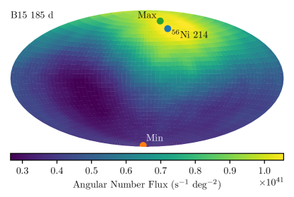
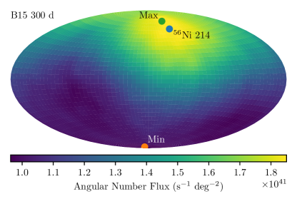
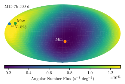
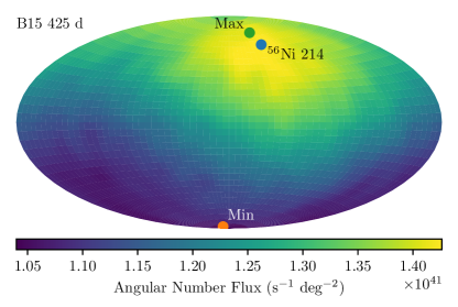
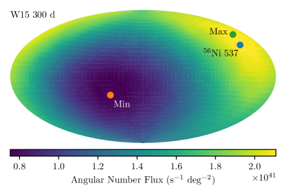
Figure 1: Spherical equal-area Hammer projections of the escaping photons at different times (for all energies). The left column shows the B15 model at three different times and the right column shows the N20, M15-7b, and W15 models at 300 d. The points show the direction of the ⁵⁶Ni center of mass (blue), minimum flux (orange), and maximum flux (green). The minimum and maximum directions are defined by the extremum number fluxes integrated over all energies and times up to 1000 d. The numbers for the ⁵⁶Ni centers of mass are the radial velocities in units of km s^-1. The distributions for narrow energy intervals are similar to the integrated distributions. The flux asymmetries are initially larger and slowly decrease as the ejecta dilute. The main difference is the difference in amplitude of the flux asymmetries, which reflects the different levels of ejecta asymmetries in the models.

Figure 1 shows spherical projections of the escape directions of the photons for the different models. All models primarily show variations on large angular scales and the brightness is correlated with the center of mass of the ⁵⁶Ni. Generally, the anisotropies are larger at early times. The temporal evolutions of all models are relatively similar and projections in narrow energy ranges show similar features. The main differences in narrow bands are that the amplitudes of the emission asymmetries are lower for low-energy photons, which have scattered many times, while the asymmetries are strongest for the line photons that escape directly (Sections 5.2 and 5.4). The scales in Figure 1 show that the N20 model is the least asymmetric whereas M15-7b is the most asymmetric model. The models that are not shown (L15, M16-7b, and IIb) show similar emission asymmetry properties. The flux ratio along the maximum to minimum direction is ${\sim}$1.7 for L15 at 300 d, ${\sim}$4 for M16-7b at 300 d, and ${\sim}$2.1 for IIb at 100 d.

In what follows, we investigate quantities averaged over all directions, as well as along the directions of minimum and maximum flux. The angle-averaged properties are a good representation of the distribution of properties over all directions (Section 6.1.1). Therefore, the angle-averaged quantities are useful, although no real observer is able to measure them. The angle-averaged properties also do not require arbitrary choices of viewing angles and are less sensitive to MC noise. Because of the directional variations are negligible on small angular scales, we use half-opening angles of 30° when computing quantities along certain directions. The extremum directions are defined by the extremum number fluxes integrated over all energies and all times ($<1000$ d).

5.2 Spectra

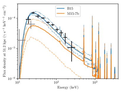
Figure 2: Spectra from the B15 and M15-7b models at 300 d (left) and direction-averaged spectra from all SN 1987A models (right). Observations of SN 1987A (crosses); HEXE at 320 d (black, Syunyaev et al. 1990), Ginga at 300 d (gray, Inoue et al. 1991), MSFC at 248 d (brown, Pendleton et al. 1995), Pulsar X-1 at 320 d (pink, Syunyaev et al. 1990), and GRIP at 268 d (yellow, Palmer et al. 1993). In the left panel, the solid lines are the spectra averaged over all directions, the semi-transparent dashed lines are along the directions of minimum flux, and the semi-transparent dash-dotted lines are along the directions of maximum flux. The envelope metallicity, which sets the low-energy cutoff, of the 10HMM model is not well-defined because metals were artificially mixed into parts of the envelope (Sections 2 and 5.6)

The left panel of Figure 2 shows the averaged and directional spectra for the B15 and M15-7b models at 300 d and the corresponding observational data. At 300 d, both the shapes and the amplitudes are in reasonable agreement with the data and any remaining deviations between models and observations can relatively easily be accommodated by the variance introduced by the asymmetries. An important property is that the asymmetries change the overall normalizations, but does not affect the shapes much. The typical amplitude of the flux variations for different viewing angles spans a factor of ${\sim}$2, but the most asymmetric model, M15-7b, shows variations up to a factor of ${\sim}$5.

The right panel of Figure 2 compares all spectra of the SN 1987A models with observational data around 300 d. We use the direction-averaged spectra and simply note that variations of a factor of a few in amplitude are possible because of asymmetries, in particular at early times (Section 6.1.1). The N20 model matches the observed spectra well but is only doing so around 300 d (Section 5.3). The 1D model 10HMM also agrees relatively well with the observations, but this required mixing introduced by hand (Section 2). This shows that 3D models are able to self-consistently produce mixing at levels similar to what is inferred from observations, whereas this had to be introduced artificially in 1D models.

The M16-7b model (red line toward the bottom of Figure 2 right) clearly fails to match the observations. We reiterate (Section 2) that M15-7b and M16-7b are presented here because they fit the X-ray and gamma-ray observations best and worst, respectively, out of the six merger progenitors that fulfill the observational criteria of the SN1987A progenitor (Menon & Heger, 2017). Out of the remaining four merger models (not shown), M15-8b and M17-7a are very similar to M16-7b, whereas M16-4a and M17-8b are intermediate cases. Only M15-7b agrees reasonably well with the X-ray and gamma-ray observations, whereas the remaining five merger models can be ruled out.

5.3 Continuum Light Curves

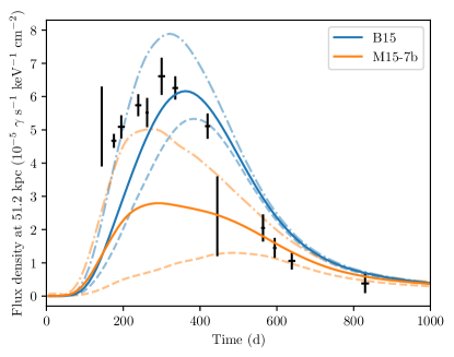
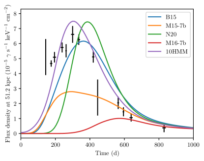
Figure 3: Light curves in the 45–105 keV range from the B15 and M15-7b models (left), direction-averaged 45–105 keV light curves from all SN 1987A models (right), and HEXE SN 1987A observations (black crosses). The horizontal bars of the data points at 145 d and 445 d are not visible because of the short exposures. In the left panel, the solid lines are averaged over all directions, the semi-transparent dashed lines are along the directions of minimum flux, and the semi-transparent dash-dotted lines are along the directions of maximum flux.

The light curves in different energy bands show similar results, but we focus on the 45–105 keV observations by HEXE because they are the most accurate. The left panel of Figure 3 shows the averaged and directional light curves for the B15 and M15-7b models in the 45–105 keV range and the corresponding HEXE data. The asymmetries clearly affect the flux magnitude and the time of the initial rise. In contrast, the declining tails are relatively similar along different directions. This is a manifestation of the emission asymmetries becoming less pronounced at later times.

The average 45–105 keV light curves for all models and the HEXE observations are shown in the right panel of Figure 3. None of the models is able to match the early observed breakout time and all overshoot the light curve at later times (except for M16-7b, which completely fails to match the observations). The general agreement with observations, however, can still be considered acceptable given the uncertainties and sensitivity of the emission properties on the progenitor structure (Section 6.2).

5.4 Line Emission

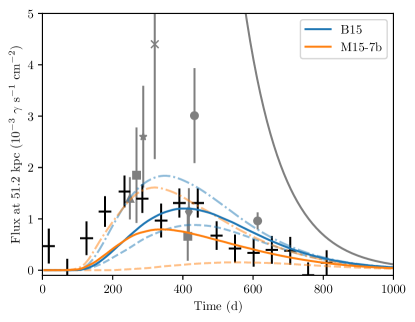
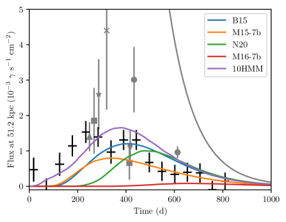
Figure 4: Temporal evolution of the sum of the 847 and 1238 keV line fluxes from the B15 and M15-7b models (left) and direction-averaged fluxes from all SN 1987A models (right). The colored solid lines that are included in the legend are direction-averaged model predictions and the gray curve is the analytic limit of free escape for 0.07 M_☉ of initial ⁵⁶Ni (Suntzeff & Bouchet, 1990; Bouchet et al., 1991). The semi-transparent dashed lines are along the minimum flux directions and the dash-dotted are along the maximum flux directions of the B15 and M15-7b models. The black crosses are SMM measurements. The gray markers are the balloon measurements; MSFC (triangle, Sandie et al. 1988b), GRIP (squares, Palmer et al. 1993), GRIS (circles, Tueller 1991), JPL (star, Mahoney et al. 1988), GRAD ($\times{}$, Rester et al. 1989), and UCR (diamond, Ait-Ouamer et al. 1992).

Figure 4 shows the line fluxes of the sum of the 847 and 1238 keV lines for the SN 1987A-like models. For the observations that only covered one of the lines, we scale that value by the atomic line yields to obtain the expected combined flux under the assumption of equal optical depths at 847 and 1238 keV. There is possibly a slight indication that the SMM measures lower fluxes than the balloon-borne experiments (Leising, 1991; Teegarden, 1994). For the comparisons with model predictions, we primarily focus on the SMM values because of the continuous coverage and homogeneity of the data.

The predicted line fluxes show the same breakout time problem as the continuum light curves. The line flux is more sensitive to the viewing angle than the continuum emission in the sense that the relative differences in flux are larger. This is because the continuum photons have scattered into new directions before escaping the ejecta, which effectively reduces the strength of the asymmetries. Apart from this, the viewing angle also affects the light curve shape for the more asymmetric models, similarly as for the continuum light curves. The accuracy of the observed line data is not as good as the continuum precision. However, the line fluxes are only functions of the optical depth along the photon path, which makes them valuable for breaking degeneracies when interpreting the more complex continuum data (Section 6.2).

5.5 Other SN Types

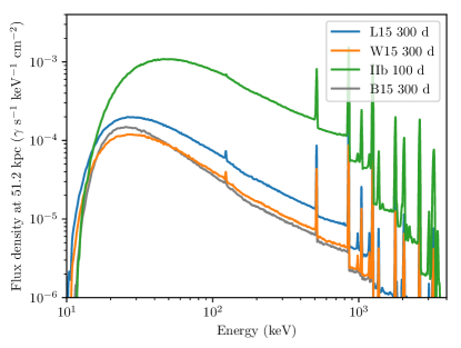
Figure 5: Direction-averaged spectra of the RSG models L15 and W15 at 300 d, and the stripped IIb model at 100 d. The gray line is the B15 model at 300 d and is included for reference. The times are chosen to be around peak flux. The variations along different directions primarily affect the magnitude of the flux while the shape remains relatively constant (Figure 2). The differences at the low-energy cutoff are primarily attributed to the different metallicities (Table 2 and Section 5.6).

We include predictions for other types of SNe as a guide for future observations. We reiterate that the masses of the radioactive elements in all models are scaled to the inferred values of SN 1987A (Section 2.2). Figure 5 shows the spectra of the RSG models L15 and W15, as well as the stripped IIb model. We note that the H-rich models are shown at 300 d, whereas the IIb model is at 100 d. This roughly corresponds to the times of peak flux. The spectral shape for a given model is softer at earlier times and harder at later times. We note that the RSG models are similar to the B15 model.

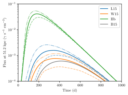
Figure 6: Temporal evolution of the 847 keV line fluxes (not the sum of the 847 and 1238 keV lines as in Figure 4) of the RSG models L15 and W15, and the stripped IIb model. The gray line is the direction-averaged line flux from the B15 model, which is included for reference. The semi-transparent dashed colored lines represent the flux along the minimum direction and the semi-transparent dash-dotted lines the flux along the maximum direction for the corresponding models.

Figure 6 shows the 847 keV line fluxes of the L15, W15, and IIb models. We also include the light curves along the extremum directions. The variations due to asymmetries are flux variations by a factor of a few but the qualitative properties of the line fluxes are independent of the viewing angle.

The most notable features of the IIb model are that it evolves faster and is more luminous at the time of peak flux than the H-rich models. This is because of the lower ejecta mass and higher expansion velocities. Furthermore, the very thin H envelope quickly becomes transparent, which shifts the photoabsorption cutoff to slightly higher energies, because the core is revealed and a larger fraction of the photons escape the ejecta before being scattered many times.

5.6 Effects of Progenitor Metallicity

In this subsection, we use five versions of the B15 model to investigate the effects of different progenitor envelope metallicities. In addition to the B15 version with LMC abundances (0.55 Z_eff,☉), we generate three additional versions of B15 with effective metallicities of 0.12, 0.27, and 1.00 Z_eff,☉. These three versions are corrected using solar abundances (Table 2.3) following the method presented in Section 2.3. Lastly, we create a fifth version with abundances corresponding to the ring of SN 1987A (Section 6.1.3), which results in an effective metallicity of 0.28 Z_eff,☉.

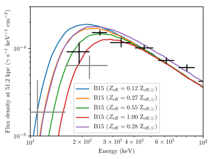
Figure 7: Spectra at 300 d for the B15 model at five different metallicities. This shows how increasing metallicity (primarily Fe abundance) of the progenitor envelope affects the low-energy photoabsorption cutoff. The green 0.55 Z_eff,☉ line is for LMC abundances and the purple 0.28 Z_eff,☉ line is for abundances of the ring of SN 1987A. The purple line deviates at higher energies because of a much higher He-to-H ratio (Section 6.1.3), which changes the Compton scattering opacity. Overplotted are the observed HEXE spectrum at 320 d (black crosses), and the Ginga bands at 300 d (gray crosses).

Figure 7 shows spectra at 300 d for the five different B15 models. This clearly shows how increasing metallicity shifts the low-energy cutoff of the spectra to higher energies by increasing the photoelectric absorption opacity. The observed SN 1987A spectra seem to align particularly well with the version with LMC metallicity, but is also consistent with abundances inferred from the ring of SN 1987A. The four versions that are practically identical at higher energies have almost the same Compton scattering opacity. This is because the metallicity corrections only involve minor changes in terms of mass, which only marginally affect the scattering opacity. The reason why the version with the SN 1987A ring abundances differs at higher energies is because of a major shift of 2.1 M_☉ of H into He (Section 6.1.3). This reduces the electron density and significantly decreases the scattering opacity. However, the cutoff is still at an energy similar to that of the version with 0.27 Z_eff,☉, which was corrected using solar abundances.

6 Discussion

6.1 General Model Emission Properties

Before comparing the predictions with the SN 1987A observations (Section 6.2), we discuss some general properties of the predicted emission. The X-ray and gamma-ray emission from different progenitors shows different properties. For a given viewing angle, the most important parameter is the electron column density outside of the fastest ⁵⁶Ni or, in other words, the amount of mixing (Section 2). This determines the time at which the first emission starts escaping the ejecta. An additional major difference between the models is that the stripped IIb model evolves on shorter timescales and is more luminous than the H-rich models because of its lower ejecta mass and higher explosion velocities.

6.1.1 Variance Due to Asymmetries

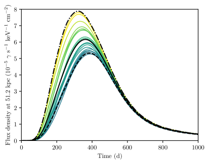
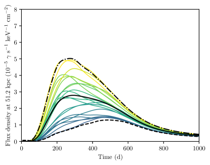
Figure 8: Light curves in the 45–105 keV range along different viewing angles for the B15 model (left) and the M15-7b model (right). The solid black lines are averaged over all directions, the dashed black lines are along the directions of minimum flux, and the dash-dotted black lines are along the directions of maximum flux. The colored lines are along 20 arbitrary uniformly distributed directions (the vertices of a dodecahedron).

First, we explore the effects of the choice of viewing angle on the observed properties. This is the variance introduced by the 3D structures for a given explosion. The variance arising from the stochastic hydrodynamic instabilities for repeated explosions of the same progenitor is investigated in Section 6.1.2.

We show the light curves in the 45–105 keV range for the B15 and M15-7b models along different viewing angles in Figure 8. The effects of the asymmetries are overall changes in amplitudes and shapes of the light curves. This is more prominent for the M15-7b model, which is the most asymmetric model. The shapes of the spectra, however, are only weakly affected (Figure 2). The general behavior of the spectral shapes along different directions is larger differences at higher energies, particularly for the direct line emission, than at lower energies. This is because the scattering effectively smooths out the asymmetries. This also implies that the line fluxes are more strongly affected by asymmetries than the 45–105 keV light curves. The peak line flux varies along different directions by more than a factor of 5 in B15 and 10 in M15-7b, and the times of peak line flux differ by up to 100 d in B15 and 300 d in M15-7b between the minimum and maximum directions.

Finally, Figure 8 clearly shows that the range of fluxes spanned by the fluxes along the minimum and maximum directions contains the fluxes from practically all directions at all times. It also shows that the angle average is a good representation of the distribution of properties over all directions.

6.1.2 Variance Due to Explosion Dynamics

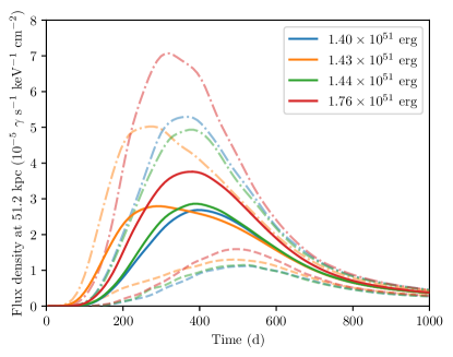
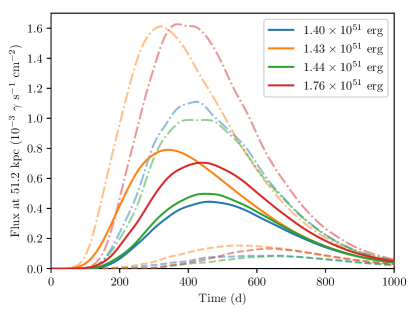
Figure 9: Light curves in the 45–105 keV range (left) and the sum of the 847 and 1238 keV line fluxes (right) from four versions of the M15-7b model with different explosion energies and seed perturbations. The orange lines are the reference M15-7b, which we focus on throughout the rest of the paper. The solid lines are averaged over all directions, the semi-transparent dashed lines are along the directions of minimum flux, and the semi-transparent dash-dotted lines are along the directions of maximum flux.

The variance introduced by the stochastic hydrodynamic evolution is seeded by the random fluctuations in the structures of the progenitors (Wongwathanarat et al., 2013). We investigate the effects on the emission properties by simulating three additional explosions of the M15-7b model. The first explosion differs by having different seed perturbations in the mapping from the 1D progenitor into three dimensions. The final explosion energy of this second model is $1.44\times{}10^{51}$ erg. The two other explosions were simulated with different seed perturbations and slightly different neutrino luminosities. They result in explosion energies of $1.40\times{}10^{51}$ and $1.76\times{}10^{51}$ erg. A similar exercise was carried out using optical light curves for three versions of the B15 model by Utrobin et al. (2015).

The 45–105 keV light curves for the four versions of M15-7b are shown in Figure 9 (left). In addition to the variance due to asymmetries of the individual models, the peak flux of the 45–105 keV continuum varies within ${\sim}$30 % and the peak time shifts by up to ${\sim}$100 d. This means that the light curve shapes are slightly different. The line fluxes (Figure 9, right) show similar variance as the continua, with the primary difference being that the angle-averaged line flux peaks span a factor of 2. For M15-7b, the differences in spectral shape resulting from the stochastic nature of the explosion are much smaller than the variance due to the intrinsic asymmetries. Finally, B15 and M15-7b can still be distinguished, despite the broad distributions of properties due to both the stochasticity of the explosions and intrinsic asymmetries (Figures 8 and 9).

6.1.3 Progenitor Metallicity

The progenitor surface metallicity also has interesting implications for the X-ray properties. Increasing progenitor metallicity shifts the low-energy X-ray cutoff to higher energies (Figure 7). This effect could potentially be used to constrain the progenitor metallicity and has previously been discussed in the context of Type Ia SNe (Maeda et al., 2012). The cutoff is also not very sensitive to the viewing angle (Figure 2) because it is determined by the properties of the outermost layers of the ejecta, which are more isotropic. On the other hand, if the homogeneity of the outer envelope is broken by large-scale convection (e.g., Hoflich 1991), it is likely that the low-energy cutoff would be less sharp, which would make it more difficult to constrain the metallicity. Inversely, this could also serve as a diagnostic of the envelope isotropy.

It is important to point out that the cutoff is only dependent on the envelope metallicity when the low-energy limit is set by photoabsorption. This is the case in the early phases during the X-ray rise. At times later than the X-ray flux peak, the escaping emission is dominated by radiation from the deeper parts where the mean atomic number is higher and photoelectric cross sections are larger. Another contributing factor (especially at very late times) is that the low-energy cutoff is determined by the ability of the ejecta to trap photons, which determines how many times photons scatter and lose energy before they escape.

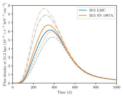
Figure 10: Light curves in the 45–105 keV range for the standard B15 version with LMC abundances (blue) and a modified B15 version with SN 1987A abundances (orange). The solid lines are averaged over all directions, the semi-transparent dashed lines are along the directions of minimum flux, and the semi-transparent dash-dotted lines are along the directions of maximum flux.

In Section 2.3, we describe the metallicity corrections for the B15 and N20 models to LMC abundances (Table 2.3). An alternative is to use the abundances of the SN 1987A progenitor inferred from observations of the equatorial ring. We check the effects on the results by comparing the B15 model with LMC abundances (that is used throughout the rest of the paper) to a B15 version with SN 1987A abundances. The 45–105 keV light curves of these models are shown in Figure 10. The line fluxes behave in a similar way. The differences are primarily driven by the increase of the of He abundance to 11.31 (0.21 relative to H by number; Lundqvist & Fransson 1996; Mattila et al. 2010) and the decrease of the Fe abundance to 6.98 ($9.6\times{}10^{-6}$ relative to H by number, Dewey et al. 2008; Zhekov et al. 2009; Mattila et al. 2010; Dewey et al. 2012). Both changes contribute to lowering the effective metallicity to 0.28 Z_eff,☉ and, consequently, shift the photoabsorption cutoff to lower energies (Figure 7). The inferred SN 1987A progenitor He abundance is more than twice as high as the LMC abundance (Table 2.3). This requires a conversion of 2.1 M_☉ of H into He in the envelope, which is a much more drastic change to the progenitor than the correction to LMC abundances. The H-to-He change lowers the scattering opacity because of the lower number of electrons per unit mass, which in turn leads to an earlier time of rise and a higher peak flux. Overall, the differences are smaller than the intrinsic asymmetries of the B15 model.

6.2 Comparisons with SN 1987A

The predictions of the B15 and M15-7b models (along the maximum direction) capture the general features of the observed data relatively well. There are, however, some significant differences that have constraining implications for the models. The other SN 1987A models are worse at reproducing the observations, primarily because of insufficient mixing of the ⁵⁶Ni to the outer layers (Table 2). The amount of mixing depends on the properties of the progenitor in a complex way and cannot be directly inferred from basic progenitor or explosion parameters (Section 2). Understanding this complex relation requires a more detailed analysis and evaluation of the growth rates of Rayleigh-Taylor instabilities for each of the models. This has been investigated for the H-rich single-star progenitors (Wongwathanarat et al., 2015; Utrobin et al., 2019), and both single stars and mergers will be presented in a forthcoming paper (V. Utrobin et al. 2019, in preparation). We do not discuss N20, M16-7b, or the other merger models (not presented) further since they all fail to match the observations.

Focusing on B15 and M15-7b, we investigate what can be inferred from the remaining differences between the model predictions and the observations. The property that is easiest to interpret is the line flux. At early times during the rising phase, this practically only depends on the column density of electrons outside the fastest trace amounts of ⁵⁶Ni on the near side. In contrast, at later times when the line fluxes are declining, they are practically only a function of the average absorption through the ejecta to the bulk of the ⁵⁶Ni. It is clear from Figure 4 that the line fluxes of all models fail to capture the early observed rise before 200 d and the fast decline after 400 d. The early-time observations most likely imply that trace amounts of ⁵⁶Ni were ejected toward us at slightly higher velocities (more strictly, higher mass coordinate) than what is seen in the models. The only other (less likely) option is that there is a thinner “hole” through the envelope that allows some emission from deeper regions to escape at early times. The late-time line observations imply that there is more material that absorbs the direct emission than predicted by the models. This can be achieved by either larger total ejecta masses or the ⁵⁶Ni being preferentially ejected toward the far side away from us.

The line fluxes are closely related to the continuum light curves. The main difference is that the continuum light curves depend non-trivially on the optical depths to the radioactive elements. For example, the continuum emission is quenched for very high absorption, as well as when approaching the optically thin regime, because the continuum requires down-scattering of line photons. In conjunction with the observations of the direct line emission, however, it is straightforward to break this degeneracy. From Figure 3, it is clear that the predicted 45–105 keV light curves fail to reach the early observed fluxes before 200 d and overshoot the observed values at times later than 400 d, similarly to the line fluxes. This results in the same constraints on the distribution of ⁵⁶Ni as discussed above, but is still helpful because the continuum data are more accurate and also provide additional independent observations.

The model spectra at 300 d in Figure 2 agree very well with observations. However, the same early deficits and late excesses that are seen in the continuum light curves (Figure 3) are of course also present in the spectra at early and late times (not shown). The difference between predicted spectra and observations at these times is primarily a change in normalization, which also implies that the continuum light curves in other energy bands show similar trends as in the presented 45–105 keV range. A notable feature in the spectra is the low-energy cutoff. It can be seen in the right panel of Figure 2 that the SN 1987A models match the spectral break around 20 keV. This is simply a manifestation of the metallicities of the progenitor envelopes (Section 5.6), which are consistent with the observed X-ray cutoff.

Finally, we stress two points concerning the magnitude of the discrepancies between the predictions and the observations. First, even though the rise of the predicted light curves are too late (left panels of Figures 3 and 4), the relative difference in maximum ⁵⁶Ni velocity required to match data is relatively low. We find that artificially increasing the radial velocity of all ⁵⁶Ni by around 20 % in the B15 model is sufficient for the direction-averaged emission to match both the low-energy continuum and line flux rise.

Secondly, the difference by a factor of ${\sim}$2 in the direct line flux around 600 d (Figure 4) can be remedied by shifting the ⁵⁶Ni center of mass. The relevant quantity is the effective optical depth and, by comparing with the free-escape asymptote in Figure 4, it is clear that only a slight increase in the optical depth is sufficient for models to match data. We make another toy model by taking the original B15 model and moving the ⁵⁶Ni center of mass from 214 to 514 km s^-1 along the same direction. This is done by applying a constant shift to all ⁵⁶Ni, effectively moving the distribution as a rigid body within the rest of the ejecta. This results in a relatively good match with observations at late times. It is only meaningful to view this model from the minimum direction because a natural consequence of the modification is that the opposite direction matches the data worse. The increased radial velocity and the center-of-mass shift of the ⁵⁶Ni distribution only marginally affect the spectral shape. It is also worth pointing out that the aforementioned example of increased mixing and center-of-mass shift is only one of many possibilities to match the data due to the large freedom when modifying 3D structures by hand.

6.3 Future Observations

We make simple predictions for observations of future nearby SNe by comparing our results with the sensitivity of current telescopes. The Chandra X-Ray Observatory (Weisskopf et al. 2000, 2002; Garmire et al. 2003) covers soft X-rays below ${\sim}10$ keV, NuSTAR covers the 3–79 keV range (Harrison et al., 2013; Madsen et al., 2015), and the spectrometer SPI (Vedrenne et al., 2003) on board the International Gamma Ray Astrophysics Laboratory (INTEGRAL, Winkler et al. 2003) extends from 20 keV to 8 MeV. Even though the effective area of XMM-Newton (Jansen et al., 2001; Strüder et al., 2001; Turner et al., 2001) is larger than the effective area of Chandra, their point source sensitivities are similar (Figure 6 of Takahashi et al. 2010). For reference, we also include the sensitivity curve of e-ASTROGAM (De Angelis et al., 2017), which was a candidate mission for the ESA M5 call and was proposed to operate from 300 keV to 3 GeV.

For the predictions, we choose a specific set of three non-stripped models and the stripped-envelope IIb model. The B15 version used for these predictions is without the metallicity correction described in Section 2.3, which means that its effective metallicity is 0.03 Z_eff,☉. The W15 model is modified to $Z_{\mathrm{eff}}=1.12$ Z_eff,☉ using solar abundances. In contrast, the metallicity of the L15 and the IIb models are unmodified from their standard values provided in Table 2. We construct this set of models to illustrate the effects of different metallicities because of its importance for the low-energy cutoff. The effects of the metallicity on the direct line fluxes are negligible.

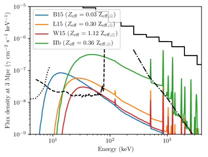
Figure 11: Comparison of predicted continua scaled to 3 Mpc with the detection sensitivities of four instruments: Chandra (dotted black line, Takahashi et al. 2010), NuSTAR (dashed black line, Koglin et al. 2005), INTEGRAL (solid black line, Roques et al. 2003), and the ESA M5 proposal e-ASTROGAM (dash-dotted black line, De Angelis et al. 2017). The spectra are at a time of 300 d for the non-stripped models and 100 d for the IIb model, which are approximately the times of peak flux in the NuSTAR band. All continuum sensitivities are given for spectral bins of $\Delta E/E=0.5$, a detection threshold of 3$\sigma$, and an exposure time of 1 Ms.

Figure 11 shows predicted spectra overplotted on the sensitivity curves of the instruments. NuSTAR is expected to provide the deepest observations. The non-stripped models are relatively similar and are expected to be detectable by NuSTAR to around 3 Mpc, whereas the limiting distance for the IIb model is around 10 Mpc. This is in agreement with the value of ${\sim}$4 Mpc given by Harrison et al. (2013) for CCSNe in general. These distances extend to slightly beyond the Local Group. It is worth pointing out that the low-metallicity version of B15 has the photoabsorption cutoff above the Chandra range (our code does not include the much fainter bremsstrahlung component at lower energies, Section 4). This means that even metal-free progenitors do not extend into the soft X-ray regime $<10$ keV.

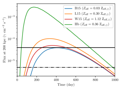
Figure 12: The 847 keV line light curves scaled to 200 kpc overplotted on the detection sensitivities of INTEGRAL/SPI (solid black line, Roques et al. 2003) and the ESA M5 proposal e-ASTROGAM (dash-dotted black line, De Angelis et al. 2017). The sensitivities are given for a detection threshold of 3$\sigma$ and an exposure time of 1 Ms.

Figure 12 shows the computed 847 keV line light curves and the narrow-line sensitivities of INTEGRAL and e-ASTROGAM. It is clear that INTEGRAL is only capable of detecting the 847 keV line out to around 200 kpc for the non-stripped SNe. This effectively limits the range to within the Milky Way and its satellites. Stripped-envelope SNe are expected to be detectable out to 2 Mpc, which covers the Local Group. e-ASTROGAM should expand the horizon by a factor of three, which would increase the number of potential targets by a factor of ${\sim}$30.

The expected CCSN rate is around 0.1 per year within 3 Mpc and 1 per year within 10 Mpc (Arnaud et al., 2004; Ando et al., 2005; Botticella et al., 2012; Horiuchi et al., 2013; Xiao & Eldridge, 2015). Inferred rates based on galaxy properties and star formation models are associated with uncertainties. Optical surveys, however, are possibly also incomplete by ${\sim}$20 % even within 10 Mpc (Prieto et al., 2012; Jencson et al., 2017, 2018; Tartaglia et al., 2018). The fraction of stripped-envelope SNe is estimated to be in the range 0.25–0.35, with reasonable agreement between estimates based on local SNe observed over the past decades (Mattila et al., 2012; Botticella et al., 2012; Horiuchi et al., 2013; Xiao & Eldridge, 2015) and surveys of larger volumes (Smartt et al., 2009; Arcavi et al., 2010; Li et al., 2011; Smith et al., 2011). Thus, a reasonable estimate is that a CCSN should be detectable by NuSTAR every three years and the most likely candidates are stripped-envelope SNe. Finally, we stress that simply comparing predicted spectra with sensitivity curves only provides a very rough estimate of what can be detected. Simulations that include detailed instrumental effects and realistic backgrounds will be the subject of future studies.

7 Summary & Conclusions

We use SN models based on 3D neutrino-driven explosion simulations (Wongwathanarat et al., 2013, 2015, 2017, M. Gabler et al. 2019, in preparation) to compute the expected early X-ray and gamma-ray emission. Four of the models are designed to represent SN 1987A; two of these are single-star BSGs and two are the results of mergers. We compare predictions from these models to observations of SN 1987A to constrain the model properties. Additionally, we investigate models of two single-star RSGs and a stripped-envelope IIb model to extend the results to other types of CCSNe that are more common than SN 1987A-like events. Our main conclusions are as follows:

1. The overall agreement between observations and model predictions indicates that the delayed neutrino-heating mechanism is able to produce SN explosions that are basically consistent with the X-ray and gamma-ray observations. General features are well reproduced, such as the normalization, spectral shape, and shape of the light curves. We stress that these models are based on realistic simulations of the progenitors and SN explosions.

2. Both the single-star progenitor B15 and the merger model M15-7b are capable of reproducing the most relevant observational X-ray and gamma-ray properties of SN 1987A. M15-7b, however, is the only progenitor out of the six merger models of Menon & Heger (2017) that is able to match the main features of the observations. Similarly, the single-star model N20 can be excluded. The primary reason for failing to match the observations is insufficient mixing of ⁵⁶Ni to the outer layers, which is related to the growth rates of Rayleigh-Taylor instabilities during the explosions (Wongwathanarat et al., 2015; Utrobin et al., 2019, V. Utrobin et al. 2019, in preparation). This also highlights that X-ray and gamma-ray observations are a powerful way of constraining progenitor models.

3. On a more detailed level, there are differences in the temporal evolution of the continuum and line fluxes between the 3D explosion models and SN 1987A observations. A suitable choice of viewing angle is not sufficient to reconcile these shortcomings. The differences can, however, be remedied by relatively small changes to the explosion dynamics. Thus, we do not consider these discrepancies to be critical issues in the explosion mechanism. Rather, they may potentially provide further insight to refine the progenitor models. For example, relative to the B15 model, it is sufficient to increase the velocity of the fastest trace amounts of ⁵⁶Ni on the near side by ${\sim}$20 %, while the bulk of the ⁵⁶Ni is redshifted by ${\sim}$500 km s^-1 instead of ${\sim}$200 km s^-1. This is only one possible explanation, which illustrates that relatively small changes to the explosion dynamics and progenitor structures are needed, especially considering the sensitivity of the dynamics to the progenitor structure. This issue will be further discussed in a follow-up paper by A. Jerkstrand et al. (2019, in preparation).

4. The low-energy spectral cutoff is determined by the photoabsorption opacity of the progenitor envelope around 30 keV. In our explosion models, the outer parts of the envelopes are relatively spherical, which means that the low-energy X-ray cutoff is insensitive to viewing angle. This is potentially a direct way of observationally constraining the composition of SN progenitors. The observations of SN 1987A are only weakly constraining and we find that the metallicity of its progenitor is consistent with both the metallicity of the LMC as well as the metallicity of its equatorial ring.

5. The asymmetries and 3D structures introduce a viewing-angle dependence, which primarily affects the overall flux normalization. For the more asymmetric models, the shapes of the light curves also change significantly for different viewing angles. The shapes of the spectra, however, remain relatively unaffected. The magnitude of these effects varies significantly depending on the level of ejecta asymmetries, epoch, and energy range considered.

6. The most important properties that affect the nature of the X-ray and gamma-ray emission are the amount of ⁵⁶Ni mixing and the level of asymmetry. Aside from this, qualitatively similar progenitor models produce relatively similar X-ray and gamma-ray emission. The X-ray and gamma-ray emission of the stripped-envelope IIb model evolves faster and is more than an order of magnitude more luminous than the non-stripped models.

7. NuSTAR offers the best prospects of future observations of early X-ray continuum emission from nearby SNe. Based on simple estimates, it should be capable of detecting non-stripped SNe within 3 Mpc and stripped-envelope SNe out to 10 Mpc, which extends to the nearest galaxies beyond the Local Group. This corresponds to an expected detection rate of 1 CCSN every three years. The deepest observations of direct line emission among the current instruments are provided by INTEGRAL/SPI. It is expected to cover non-stripped SNe in the Milky Way and its satellites, and reach stripped SNe at 2 Mpc, which is comparable to the extent of the Local Group.

References

- Ait-Ouamer et al. (1992) Ait-Ouamer, F., Kerrick, A. D., O’Neill, T. J., et al. 1992, ApJ, 386, 715, doi: 10.1086/171052
- Alp et al. (2018) Alp, D., Larsson, J., Fransson, C., et al. 2018, ApJ, 864, 175, doi: 10.3847/1538-4357/aad737
- Althouse et al. (1985) Althouse, W. E., Cook, W. R., Cummings, A. C., et al. 1985, International Cosmic Ray Conference, 3
- Ambwani & Sutherland (1988) Ambwani, K., & Sutherland, P. 1988, ApJ, 325, 820, doi: 10.1086/166052
- Anderson (2019) Anderson, J. P. 2019, arXiv e-prints, arXiv:1906.00761. https://arxiv.org/abs/1906.00761
- Ando et al. (2005) Ando, S., Beacom, J. F., & Yüksel, H. 2005, Physical Review Letters, 95, 171101, doi: 10.1103/PhysRevLett.95.171101
- Arcavi et al. (2010) Arcavi, I., Gal-Yam, A., Kasliwal, M. M., et al. 2010, ApJ, 721, 777, doi: 10.1088/0004-637X/721/1/777
- Arnaud et al. (2004) Arnaud, N., Barsuglia, M., Bizouard, M.-A., et al. 2004, Astroparticle Physics, 21, 201, doi: 10.1016/j.astropartphys.2003.12.005
- Arnett (1966) Arnett, W. D. 1966, Canadian Journal of Physics, 44, 2553, doi: 10.1139/p66-210
- Arnett et al. (1989) Arnett, W. D., Bahcall, J. N., Kirshner, R. P., & Woosley, S. E. 1989, ARA&A, 27, 629, doi: 10.1146/annurev.aa.27.090189.003213
- Astropy Collaboration et al. (2013) Astropy Collaboration, Robitaille, T. P., Tollerud, E. J., et al. 2013, A&A, 558, A33, doi: 10.1051/0004-6361/201322068
- Baade & Zwicky (1934) Baade, W., & Zwicky, F. 1934, Proceedings of the National Academy of Science, 20, 259, doi: 10.1073/pnas.20.5.259
- Barthelmy et al. (1991) Barthelmy, S., Gehrels, N., Teegarden, B. J., et al. 1991, in American Institute of Physics Conference Series, Vol. 232, Gamma-Ray Line Astrophysics, ed. P. Durouchoux & N. Prantzos, 205–210
- Bethe (1990) Bethe, H. A. 1990, Reviews of Modern Physics, 62, 801, doi: 10.1103/RevModPhys.62.801
- Bethe & Pizzochero (1990) Bethe, H. A., & Pizzochero, P. 1990, ApJ, 350, L33, doi: 10.1086/185661
- Bethe & Wilson (1985) Bethe, H. A., & Wilson, J. R. 1985, ApJ, 295, 14, doi: 10.1086/163343
- Bhat (1992) Bhat, M. R. 1992, Nuclear Data Sheets, 67, 195, doi: 10.1016/0090-3752(92)80020-K
- Bhat (1998) —. 1998, Nuclear Data Sheets, 85, 415, doi: 10.1006/ndsh.1998.0021
- Blackburn (1995) Blackburn, J. K. 1995, in Astronomical Society of the Pacific Conference Series, Vol. 77, Astronomical Data Analysis Software and Systems IV, ed. R. A. Shaw, H. E. Payne, & J. J. E. Hayes, 367
- Blinnikov et al. (2000) Blinnikov, S., Lundqvist, P., Bartunov, O., Nomoto, K., & Iwamoto, K. 2000, ApJ, 532, 1132, doi: 10.1086/308588
- Botticella et al. (2012) Botticella, M. T., Smartt, S. J., Kennicutt, R. C., et al. 2012, A&A, 537, A132, doi: 10.1051/0004-6361/201117343
- Bouchet et al. (1991) Bouchet, P., Phillips, M. M., Suntzeff, N. B., et al. 1991, A&A, 245, 490
- Bruenn (1985) Bruenn, S. W. 1985, ApJS, 58, 771, doi: 10.1086/191056
- Bruenn (1993) Bruenn, S. W. 1993, in Nuclear Physics in the Universe, ed. M. W. Guidry & M. R. Strayer, 31–50
- Bunner (1988) Bunner, A. N. 1988, in American Institute of Physics Conference Series, Vol. 170, Nuclear Spectroscopy of Astrophysical Sources, ed. N. Gehrels & G. H. Share, 43–50
- Buras et al. (2006) Buras, R., Rampp, M., Janka, H. T., & Kifonidis, K. 2006, A&A, 447, 1049, doi: 10.1051/0004-6361:20053783
- Burbidge et al. (1957) Burbidge, E. M., Burbidge, G. R., Fowler, W. A., & Hoyle, F. 1957, Reviews of Modern Physics, 29, 547, doi: 10.1103/RevModPhys.29.547
- Burrows (2013) Burrows, A. 2013, Reviews of Modern Physics, 85, 245, doi: 10.1103/RevModPhys.85.245
- Burrows & The (1990) Burrows, A., & The, L.-S. 1990, ApJ, 360, 626, doi: 10.1086/169150
- Burrows & van Riper (1995) Burrows, A., & van Riper, K. A. 1995, ApJ, 455, 215, doi: 10.1086/176569
- Chevalier & Fransson (1994) Chevalier, R. A., & Fransson, C. 1994, ApJ, 420, 268, doi: 10.1086/173557
- Chevalier & Fransson (2017) —. 2017, Thermal and Non-thermal Emission from Circumstellar Interaction (Springer International Publishing AG), 875
- Chevalier & Irwin (2012) Chevalier, R. A., & Irwin, C. M. 2012, ApJ, 747, L17, doi: 10.1088/2041-8205/747/1/L17
- Chugai et al. (1997) Chugai, N. N., Chevalier, R. A., Kirshner, R. P., & Challis, P. M. 1997, ApJ, 483, 925, doi: 10.1086/304253
- Clayton (1974) Clayton, D. D. 1974, ApJ, 188, 155, doi: 10.1086/152698
- Clayton et al. (1969) Clayton, D. D., Colgate, S. A., & Fishman, G. J. 1969, ApJ, 155, 75, doi: 10.1086/149849
- Clayton & The (1991) Clayton, D. D., & The, L.-S. 1991, ApJ, 375, 221, doi: 10.1086/170184
- Colgate & White (1966) Colgate, S. A., & White, R. H. 1966, ApJ, 143, 626, doi: 10.1086/148549
- Collette (2013) Collette, A. 2013, Python and HDF5: Unlocking Scientific Data (O’Reilly Media). https://books.google.se/books?id=1RaMAQAAQBAJ
- Cook et al. (1988) Cook, W. R., Palmer, D. M., Prince, T. A., et al. 1988, ApJ, 334, L87, doi: 10.1086/185318
- Couch (2017) Couch, S. M. 2017, Philosophical Transactions of the Royal Society of London Series A, 375, 20160271, doi: 10.1098/rsta.2016.0271
- De Angelis et al. (2017) De Angelis, A., Tatischeff, V., Tavani, M., et al. 2017, Experimental Astronomy, 44, 25, doi: 10.1007/s10686-017-9533-6
- Dewey et al. (2012) Dewey, D., Dwarkadas, V. V., Haberl, F., Sturm, R., & Canizares, C. R. 2012, ApJ, 752, 103, doi: 10.1088/0004-637X/752/2/103
- Dewey et al. (2008) Dewey, D., Zhekov, S. A., McCray, R., & Canizares, C. R. 2008, ApJ, 676, L131, doi: 10.1086/587549
- Dotani et al. (1987) Dotani, T., Hayashida, K., Inoue, H., et al. 1987, Nature, 330, 230, doi: 10.1038/330230a0
- Dwarkadas (2014) Dwarkadas, V. V. 2014, MNRAS, 440, 1917, doi: 10.1093/mnras/stu347
- Firestone et al. (1999) Firestone, R. B., Ekstrom, L. P., & Chu, S. Y. F. 1999, in APS Division of Nuclear Physics Meeting Abstracts, CE.13
- Fishman et al. (1990) Fishman, G. J., Wilson, R. B., Paciesas, W. S., et al. 1990, Advances in Space Research, 10, 55, doi: 10.1016/0273-1177(90)90118-J
- Forrest et al. (1980) Forrest, D. J., Chupp, E. L., Ryan, J. M., et al. 1980, Sol. Phys., 65, 15, doi: 10.1007/BF00151381
- Fowler & Hoyle (1964) Fowler, W. A., & Hoyle, F. 1964, ApJS, 9, 201, doi: 10.1086/190103
- Frank et al. (2016) Frank, K. A., Zhekov, S. A., Park, S., et al. 2016, ApJ, 829, 40, doi: 10.3847/0004-637X/829/1/40
- Fransson & Kozma (1993) Fransson, C., & Kozma, C. 1993, ApJ, 408, L25, doi: 10.1086/186822
- Fransson et al. (1996) Fransson, C., Lundqvist, P., & Chevalier, R. A. 1996, ApJ, 461, 993, doi: 10.1086/177119
- Fransson et al. (2013) Fransson, C., Larsson, J., Spyromilio, J., et al. 2013, ApJ, 768, 88, doi: 10.1088/0004-637X/768/1/88
- Fryxell et al. (1991) Fryxell, B., Arnett, D., & Mueller, E. 1991, ApJ, 367, 619, doi: 10.1086/169657
- Garmire et al. (2003) Garmire, G. P., Bautz, M. W., Ford, P. G., Nousek, J. A., & Ricker, Jr., G. R. 2003, in Proc. SPIE, Vol. 4851, X-Ray and Gamma-Ray Telescopes and Instruments for Astronomy., ed. J. E. Truemper & H. D. Tananbaum, 28–44
- Gehrels et al. (1988) Gehrels, N., Leventhal, M., & MacCallum, C. J. 1988, in American Institute of Physics Conference Series, Vol. 170, Nuclear Spectroscopy of Astrophysical Sources, ed. N. Gehrels & G. H. Share, 87–95
- Gould & Uza (1998) Gould, A., & Uza, O. 1998, ApJ, 494, 118, doi: 10.1086/305193
- Gröningsson et al. (2008a) Gröningsson, P., Fransson, C., Leibundgut, B., et al. 2008a, A&A, 492, 481, doi: 10.1051/0004-6361:200810551
- Gröningsson et al. (2008b) Gröningsson, P., Fransson, C., Lundqvist, P., et al. 2008b, A&A, 479, 761, doi: 10.1051/0004-6361:20077604
- Harrison et al. (2013) Harrison, F. A., Craig, W. W., Christensen, F. E., et al. 2013, ApJ, 770, 103, doi: 10.1088/0004-637X/770/2/103
- Hillier & Dessart (2012) Hillier, D. J., & Dessart, L. 2012, MNRAS, 424, 252, doi: 10.1111/j.1365-2966.2012.21192.x
- Hix & Harris (2017) Hix, W. R., & Harris, J. A. 2017, in Handbook of Supernovae, ISBN 978-3-319-21845-8. Springer International Publishing AG, 2017, p. 1771, ed. A. W. Alsabti & P. Murdin, 1771
- Hoeflich et al. (1992) Hoeflich, P., Khokhlov, A., & Mueller, E. 1992, A&A, 259, 549
- Hoflich (1991) Hoflich, P. 1991, A&A, 246, 481
- Höflich (2002) Höflich, P. 2002, New A Rev., 46, 475, doi: 10.1016/S1387-6473(02)00186-0
- Horiuchi et al. (2013) Horiuchi, S., Beacom, J. F., Bothwell, M. S., & Thompson, T. A. 2013, ApJ, 769, 113, doi: 10.1088/0004-637X/769/2/113
- Hotokezaka et al. (2016) Hotokezaka, K., Wanajo, S., Tanaka, M., et al. 2016, MNRAS, 459, 35, doi: 10.1093/mnras/stw404
- Hoyle (1954) Hoyle, F. 1954, ApJS, 1, 121, doi: 10.1086/190005
- Hoyle & Fowler (1960) Hoyle, F., & Fowler, W. A. 1960, ApJ, 132, 565, doi: 10.1086/146963
- Hubbell (1969) Hubbell, J. 1969, National Bureau of Standards Report NSRDS-NBS29, Washington DC
- Hubbell et al. (1980) Hubbell, J. H., Gimm, H. A., & Øverbø, I. 1980, Journal of Physical and Chemical Reference Data, 9, 1023, doi: 10.1063/1.555629
- Hungerford et al. (2005) Hungerford, A. L., Fryer, C. L., & Rockefeller, G. 2005, ApJ, 635, 487, doi: 10.1086/497323
- Hungerford et al. (2003) Hungerford, A. L., Fryer, C. L., & Warren, M. S. 2003, ApJ, 594, 390, doi: 10.1086/376776
- Hunter et al. (2007) Hunter, I., Dufton, P. L., Smartt, S. J., et al. 2007, A&A, 466, 277, doi: 10.1051/0004-6361:20066148
- Hunter (2007) Hunter, J. D. 2007, Computing in Science and Engineering, 9, 90, doi: 10.1109/MCSE.2007.55
- Inoue et al. (1991) Inoue, H., Hayashida, K., Itoh, M., et al. 1991, PASJ, 43, 213
- Janka (2012) Janka, H.-T. 2012, Annual Review of Nuclear and Particle Science, 62, 407, doi: 10.1146/annurev-nucl-102711-094901
- Janka (2017) —. 2017, Neutrino-Driven Explosions (Springer International Publishing AG), 1095
- Janka et al. (2016) Janka, H.-T., Melson, T., & Summa, A. 2016, Annual Review of Nuclear and Particle Science, 66, 341, doi: 10.1146/annurev-nucl-102115-044747
- Jansen et al. (2001) Jansen, F., Lumb, D., Altieri, B., et al. 2001, A&A, 365, L1, doi: 10.1051/0004-6361:20000036
- Jencson et al. (2017) Jencson, J. E., Kasliwal, M. M., Johansson, J., et al. 2017, ApJ, 837, 167, doi: 10.3847/1538-4357/aa618f
- Jencson et al. (2018) Jencson, J. E., Kasliwal, M. M., Adams, S. M., et al. 2018, ApJ, 863, 20, doi: 10.3847/1538-4357/aacf8b
- Jerkstrand et al. (2011) Jerkstrand, A., Fransson, C., & Kozma, C. 2011, A&A, 530, A45, doi: 10.1051/0004-6361/201015937
- Jerkstrand et al. (2016) Jerkstrand, A., Smartt, S. J., & Heger, A. 2016, MNRAS, 455, 3207, doi: 10.1093/mnras/stv2369
- Jones et al. (2001–) Jones, E., Oliphant, T., Peterson, P., et al. 2001–
- Joye & Mandel (2003) Joye, W. A., & Mandel, E. 2003, in Astronomical Society of the Pacific Conference Series, Vol. 295, Astronomical Data Analysis Software and Systems XII, ed. H. E. Payne, R. I. Jedrzejewski, & R. N. Hook, 489
- Junde (1992) Junde, H. 1992, Nuclear Data Sheets, 67, 523, doi: 10.1016/0090-3752(92)80026-G
- Junde (1999) —. 1999, Nuclear Data Sheets, 86, 315, doi: 10.1006/ndsh.1999.0004
- Junde et al. (2011) Junde, H., Su, H., & Dong, Y. 2011, Nuclear Data Sheets, 112, 1513, doi: 10.1016/j.nds.2011.04.004
- Kageyama & Sato (2004) Kageyama, A., & Sato, T. 2004, Geochemistry, Geophysics, Geosystems, 5, Q09005, doi: 10.1029/2004GC000734
- Kasen & Woosley (2009) Kasen, D., & Woosley, S. E. 2009, ApJ, 703, 2205, doi: 10.1088/0004-637X/703/2/2205
- Kifonidis et al. (2003) Kifonidis, K., Plewa, T., Janka, H.-T., & Müller, E. 2003, A&A, 408, 621, doi: 10.1051/0004-6361:20030863
- Koglin et al. (2005) Koglin, J. E., Christensen, F. E., Craig, W. W., et al. 2005, in Proc. SPIE, Vol. 5900, Optics for EUV, X-Ray, and Gamma-Ray Astronomy II, ed. O. Citterio & S. L. O’Dell, 266–275
- Korobkin et al. (2019) Korobkin, O., Hungerford, A. M., Fryer, C. L., et al. 2019, arXiv e-prints, arXiv:1905.05089. https://arxiv.org/abs/1905.05089
- Kromer & Sim (2009) Kromer, M., & Sim, S. A. 2009, MNRAS, 398, 1809, doi: 10.1111/j.1365-2966.2009.15256.x
- Kurfess et al. (1992) Kurfess, J. D., Johnson, W. N., Kinzer, R. L., et al. 1992, ApJ, 399, L137, doi: 10.1086/186626
- Kurt & Dufour (1998) Kurt, C. M., & Dufour, R. J. 1998, in Revista Mexicana de Astronomia y Astrofisica Conference Series, Vol. 7, Revista Mexicana de Astronomia y Astrofisica Conference Series, ed. R. J. Dufour & S. Torres-Peimbert, 202
- Leising (1989) Leising, M. D. 1989, in Cosmic Gamma Rays and Cosmic Neutrinos, ed. M. M. Shapiro & J. P. Wefel, 321–328
- Leising (1991) Leising, M. D. 1991, Advances in Space Research, 11, 207, doi: 10.1016/0273-1177(91)90173-H
- Leising & Share (1990) Leising, M. D., & Share, G. H. 1990, ApJ, 357, 638, doi: 10.1086/168952
- Leising et al. (1994) Leising, M. D., Kurfess, J. D., Clayton, D. D., et al. 1994, ApJ, 431, L95, doi: 10.1086/187481
- Li et al. (2011) Li, W., Leaman, J., Chornock, R., et al. 2011, MNRAS, 412, 1441, doi: 10.1111/j.1365-2966.2011.18160.x
- Limongi et al. (2000) Limongi, M., Straniero, O., & Chieffi, A. 2000, ApJS, 129, 625, doi: 10.1086/313424
- Lodders (2003) Lodders, K. 2003, ApJ, 591, 1220, doi: 10.1086/375492
- Lundqvist & Fransson (1996) Lundqvist, P., & Fransson, C. 1996, ApJ, 464, 924, doi: 10.1086/177380
- Madsen et al. (2015) Madsen, K. K., Harrison, F. A., Markwardt, C. B., et al. 2015, ApJS, 220, 8, doi: 10.1088/0067-0049/220/1/8
- Maeda (2006) Maeda, K. 2006, ApJ, 644, 385, doi: 10.1086/503415
- Maeda et al. (2014) Maeda, K., Kutsuna, M., & Shigeyama, T. 2014, ApJ, 794, 37, doi: 10.1088/0004-637X/794/1/37
- Maeda et al. (2012) Maeda, K., Terada, Y., Kasen, D., et al. 2012, ApJ, 760, 54, doi: 10.1088/0004-637X/760/1/54
- Mahoney et al. (1988) Mahoney, W. A., Varnell, L. S., Jacobson, A. S., et al. 1988, ApJ, 334, L81, doi: 10.1086/185317
- Makino & ASTRO-C Team (1987) Makino, F., & ASTRO-C Team. 1987, Astrophys. Lett., 25, 223
- Mattila et al. (2010) Mattila, S., Lundqvist, P., Gröningsson, P., et al. 2010, ApJ, 717, 1140, doi: 10.1088/0004-637X/717/2/1140
- Mattila et al. (2012) Mattila, S., Dahlen, T., Efstathiou, A., et al. 2012, ApJ, 756, 111, doi: 10.1088/0004-637X/756/2/111
- Matz et al. (1988) Matz, S. M., Share, G. H., Leising, M. D., Chupp, E. L., & Vestrand, W. T. 1988, Nature, 331, 416, doi: 10.1038/331416a0
- McCray (1993) McCray, R. 1993, ARA&A, 31, 175, doi: 10.1146/annurev.aa.31.090193.001135
- McCray & Fransson (2016) McCray, R., & Fransson, C. 2016, ARA&A, 54, 19, doi: 10.1146/annurev-astro-082615-105405
- Menon & Heger (2017) Menon, A., & Heger, A. 2017, MNRAS, 469, 4649, doi: 10.1093/mnras/stx818
- Menon et al. (2019) Menon, A., Utrobin, V., & Heger, A. 2019, MNRAS, 482, 438, doi: 10.1093/mnras/sty2647
- Milne et al. (2004) Milne, P. A., Hungerford, A. L., Fryer, C. L., et al. 2004, ApJ, 613, 1101, doi: 10.1086/423235
- Mitchell et al. (2002) Mitchell, R. C., Baron, E., Branch, D., et al. 2002, ApJ, 574, 293, doi: 10.1086/340928
- Müller (2016) Müller, B. 2016, PASA, 33, e048, doi: 10.1017/pasa.2016.40
- Müller et al. (1991) Müller, E., Fryxell, B., & Arnett, D. 1991, A&A, 251, 505
- Müller et al. (2017) Müller, T., Prieto, J. L., Pejcha, O., & Clocchiatti, A. 2017, ApJ, 841, 127, doi: 10.3847/1538-4357/aa72f1
- Nasa High Energy Astrophysics Science Archive Research Center (2014) (Heasarc) Nasa High Energy Astrophysics Science Archive Research Center (Heasarc). 2014, HEAsoft: Unified Release of FTOOLS and XANADU, Astrophysics Source Code Library. http://ascl.net/1408.004
- Nomoto & Hashimoto (1988) Nomoto, K., & Hashimoto, M. 1988, Phys. Rep., 163, 13, doi: 10.1016/0370-1573(88)90032-4
- Nomoto et al. (1984) Nomoto, K., Thielemann, F.-K., & Yokoi, K. 1984, ApJ, 286, 644, doi: 10.1086/162639
- Ofek et al. (2014) Ofek, E. O., Zoglauer, A., Boggs, S. E., et al. 2014, ApJ, 781, 42, doi: 10.1088/0004-637X/781/1/42
- Palmer et al. (1993) Palmer, D. M., Schindler, S. M., Cook, W. R., et al. 1993, ApJ, 412, 203, doi: 10.1086/172912
- Panagia (1999) Panagia, N. 1999, in IAU Symposium, Vol. 190, New Views of the Magellanic Clouds, ed. Y.-H. Chu, N. Suntzeff, J. Hesser, & D. Bohlender, 549
- Panagia et al. (1991) Panagia, N., Gilmozzi, R., Macchetto, F., Adorf, H.-M., & Kirshner, R. P. 1991, ApJ, 380, L23, doi: 10.1086/186164
- Pejcha & Prieto (2015) Pejcha, O., & Prieto, J. L. 2015, ApJ, 806, 225, doi: 10.1088/0004-637X/806/2/225
- Pendleton et al. (1995) Pendleton, G. N., Paciesas, W. S., Fishman, G. J., Meegan, C. A., & Wilson, R. B. 1995, ApJ, 439, 963, doi: 10.1086/175233
- Pinto & Woosley (1988) Pinto, P. A., & Woosley, S. E. 1988, Nature, 333, 534, doi: 10.1038/333534a0
- Pozdnyakov et al. (1983) Pozdnyakov, L. A., Sobol, I. M., & Syunyaev, R. A. 1983, Astrophysics and Space Physics Reviews, 2, 189
- Prieto et al. (2012) Prieto, J. L., Lee, J. C., Drake, A. J., et al. 2012, ApJ, 745, 70, doi: 10.1088/0004-637X/745/1/70
- Rampp & Janka (2002) Rampp, M., & Janka, H.-T. 2002, A&A, 396, 361, doi: 10.1051/0004-6361:20021398
- Rester et al. (1989) Rester, A. C., Coldwell, R. L., Dunnam, F. E., et al. 1989, ApJ, 342, L71, doi: 10.1086/185487
- Roques et al. (2003) Roques, J. P., Schanne, S., von Kienlin, A., et al. 2003, A&A, 411, L91, doi: 10.1051/0004-6361:20031501
- Ruiz-Lapuente & Spruit (1998) Ruiz-Lapuente, P., & Spruit, H. C. 1998, ApJ, 500, 360, doi: 10.1086/305697
- Russell & Bessell (1989) Russell, S. C., & Bessell, M. S. 1989, ApJS, 70, 865, doi: 10.1086/191360
- Russell & Dopita (1990) Russell, S. C., & Dopita, M. A. 1990, ApJS, 74, 93, doi: 10.1086/191494
- Russell & Dopita (1992) —. 1992, ApJ, 384, 508, doi: 10.1086/170893
- Rybicki & Lightman (1979) Rybicki, G. B., & Lightman, A. P. 1979, Radiative processes in astrophysics (New York, Wiley-Interscience)
- Saio et al. (1988) Saio, H., Nomoto, K., & Kato, M. 1988, Nature, 334, 508, doi: 10.1038/334508a0
- Sandie et al. (1988a) Sandie, W. G., Nakano, G. H., Chase, Jr., L. F., et al. 1988a, in Supernova 1987A in the Large Magellanic Cloud, ed. M. Kafatos & A. G. Michalitsianos, 366–370
- Sandie et al. (1988b) Sandie, W. G., Nakano, G. H., Chase, Jr., L. F., et al. 1988b, ApJ, 334, L91, doi: 10.1086/185319
- Santana et al. (2016) Santana, R., Crumley, P., Hernández, R. A., & Kumar, P. 2016, MNRAS, 456, 1049, doi: 10.1093/mnras/stv2709
- Shigeyama & Nomoto (1990) Shigeyama, T., & Nomoto, K. 1990, ApJ, 360, 242, doi: 10.1086/169114
- Sim (2007) Sim, S. A. 2007, MNRAS, 375, 154, doi: 10.1111/j.1365-2966.2006.11271.x
- Sim & Mazzali (2008) Sim, S. A., & Mazzali, P. A. 2008, MNRAS, 385, 1681, doi: 10.1111/j.1365-2966.2008.12600.x
- Simone et al. (1985) Simone, J., Oneill, T., Tumer, O. T., & Zych, A. D. 1985, IEEE Transactions on Nuclear Science, 32, 124, doi: 10.1109/TNS.1985.4336806
- Smartt et al. (2009) Smartt, S. J., Eldridge, J. J., Crockett, R. M., & Maund, J. R. 2009, MNRAS, 395, 1409, doi: 10.1111/j.1365-2966.2009.14506.x
- Smith et al. (2011) Smith, N., Li, W., Filippenko, A. V., & Chornock, R. 2011, MNRAS, 412, 1522, doi: 10.1111/j.1365-2966.2011.17229.x
- Strüder et al. (2001) Strüder, L., Briel, U., Dennerl, K., et al. 2001, A&A, 365, L18, doi: 10.1051/0004-6361:20000066
- Summa et al. (2013) Summa, A., Ulyanov, A., Kromer, M., et al. 2013, A&A, 554, A67, doi: 10.1051/0004-6361/201220972
- Suntzeff & Bouchet (1990) Suntzeff, N. B., & Bouchet, P. 1990, AJ, 99, 650, doi: 10.1086/115358
- Sunyaev et al. (1987) Sunyaev, R., Kaniovsky, A., Efremov, V., et al. 1987, Nature, 330, 227, doi: 10.1038/330227a0
- Sunyaev et al. (1991) Sunyaev, R., Grebenev, S., Kaniovsky, A., et al. 1991, in American Institute of Physics Conference Series, Vol. 232, Gamma-Ray Line Astrophysics, ed. P. Durouchoux & N. Prantzos, 211–217
- Swartz et al. (1995) Swartz, D. A., Sutherland, P. G., & Harkness, R. P. 1995, ApJ, 446, 766, doi: 10.1086/175834
- Syunyaev et al. (1987) Syunyaev, R. A., Kaniovskii, A., Efremov, V., et al. 1987, Soviet Astronomy Letters, 13, 431
- Syunyaev et al. (1988) Syunyaev, R. A., Efremov, V. V., Kaniovskii, A. S., et al. 1988, Soviet Astronomy Letters, 14, 247
- Syunyaev et al. (1989) Syunyaev, R. A., Kaniovskii, A. S., Efremov, V. V., et al. 1989, Soviet Astronomy Letters, 15, 125
- Syunyaev et al. (1990) —. 1990, Soviet Astronomy Letters, 16, 171
- Taddia et al. (2018) Taddia, F., Stritzinger, M. D., Bersten, M., et al. 2018, A&A, 609, A136, doi: 10.1051/0004-6361/201730844
- Takahashi et al. (2010) Takahashi, T., Mitsuda, K., & Kelley, R. 2010, X-ray Astronomy 2009; Present Status, Multi-Wavelength Approach and Future Perspectives, 1248, 537, doi: 10.1063/1.3475335
- Tanaka (1988) Tanaka, Y. 1988, in Lecture Notes in Physics, Berlin Springer Verlag, Vol. 305, IAU Colloq. 108: Atmospheric Diagnostics of Stellar Evolution, ed. K. Nomoto, 399
- Tanaka (1991) Tanaka, Y. 1991, in Supernovae, ed. S. E. Woosley, 269
- Tartaglia et al. (2018) Tartaglia, L., Sand, D. J., Valenti, S., et al. 2018, ApJ, 853, 62, doi: 10.3847/1538-4357/aaa014
- Teegarden (1991) Teegarden, B. J. 1991, Advances in Space Research, 11, 217, doi: 10.1016/0273-1177(91)90174-I
- Teegarden (1994) —. 1994, ApJS, 92, 363, doi: 10.1086/191979
- Teegarden et al. (1989) Teegarden, B. J., Barthelmy, S. D., Gehrels, N., Tueller, J., & Leventhal, M. 1989, Nature, 339, 122, doi: 10.1038/339122a0
- The & Burrows (2014) The, L.-S., & Burrows, A. 2014, ApJ, 786, 141, doi: 10.1088/0004-637X/786/2/141
- Thielemann et al. (1990) Thielemann, F.-K., Hashimoto, M.-A., & Nomoto, K. 1990, ApJ, 349, 222, doi: 10.1086/168308
- Truelove & McKee (1999) Truelove, J. K., & McKee, C. F. 1999, ApJS, 120, 299, doi: 10.1086/313176
- Trundle et al. (2007) Trundle, C., Dufton, P. L., Hunter, I., et al. 2007, A&A, 471, 625, doi: 10.1051/0004-6361:20077838
- Tueller (1991) Tueller, J. 1991, in American Institute of Physics Conference Series, Vol. 232, Gamma-Ray Line Astrophysics, ed. P. Durouchoux & N. Prantzos, 199–204
- Tueller et al. (1991) Tueller, J., Barthelmy, S., Gehrels, N., et al. 1991, in Supernovae, ed. S. E. Woosley, 278
- Tueller et al. (1990) Tueller, J., Barthelmy, S., Gehrels, N., et al. 1990, ApJ, 351, L41, doi: 10.1086/185675
- Turner et al. (2001) Turner, M. J. L., Abbey, A., Arnaud, M., et al. 2001, A&A, 365, L27, doi: 10.1051/0004-6361:20000087
- Utrobin (2005) Utrobin, V. P. 2005, Astronomy Letters, 31, 806, doi: 10.1134/1.2138767
- Utrobin et al. (2015) Utrobin, V. P., Wongwathanarat, A., Janka, H.-T., & Müller, E. 2015, A&A, 581, A40, doi: 10.1051/0004-6361/201425513
- Utrobin et al. (2019) Utrobin, V. P., Wongwathanarat, A., Janka, H.-T., et al. 2019, A&A, 624, A116, doi: 10.1051/0004-6361/201834976
- van der Walt et al. (2011) van der Walt, S., Colbert, S. C., & Varoquaux, G. 2011, Computing in Science Engineering, 13, 22, doi: 10.1109/MCSE.2011.37
- Vedrenne et al. (2003) Vedrenne, G., Roques, J.-P., Schönfelder, V., et al. 2003, A&A, 411, L63, doi: 10.1051/0004-6361:20031482
- Veigele (1973) Veigele, W. J. 1973, Atomic Data, 5, 51, doi: 10.1016/S0092-640X(73)80015-4
- Verner et al. (1996) Verner, D. A., Ferland, G. J., Korista, K. T., & Yakovlev, D. G. 1996, ApJ, 465, 487, doi: 10.1086/177435
- Verner & Yakovlev (1995) Verner, D. A., & Yakovlev, D. G. 1995, A&AS, 109, 125
- Wamsteker (1993) Wamsteker, W. 1993, in Lecture Notes in Physics, Berlin Springer Verlag, Vol. 416, New Aspects of Magellanic Cloud Research, ed. B. Baschek, G. Klare, & J. Lequeux, 199–207
- Weisskopf et al. (2002) Weisskopf, M. C., Brinkman, B., Canizares, C., et al. 2002, PASP, 114, 1, doi: 10.1086/338108
- Weisskopf et al. (2000) Weisskopf, M. C., Tananbaum, H. D., Van Speybroeck, L. P., & O’Dell, S. L. 2000, in Proc. SPIE, Vol. 4012, X-Ray Optics, Instruments, and Missions III, ed. J. E. Truemper & B. Aschenbach, 2–16
- Willingale et al. (2013) Willingale, R., Starling, R. L. C., Beardmore, A. P., Tanvir, N. R., & O’Brien, P. T. 2013, MNRAS, 431, 394, doi: 10.1093/mnras/stt175
- Wilson et al. (1988) Wilson, R. B., Fishman, G. J., Meegan, C. A., Paciesas, W. S., & Pendleton, G. N. 1988, in American Institute of Physics Conference Series, Vol. 170, Nuclear Spectroscopy of Astrophysical Sources, ed. N. Gehrels & G. H. Share, 73–79
- Winkler et al. (2003) Winkler, C., Courvoisier, T. J.-L., Di Cocco, G., et al. 2003, A&A, 411, L1, doi: 10.1051/0004-6361:20031288
- Wollaeger et al. (2017) Wollaeger, R. T., Hungerford, A. L., Fryer, C. L., et al. 2017, ApJ, 845, 168, doi: 10.3847/1538-4357/aa82bd
- Wongwathanarat et al. (2010) Wongwathanarat, A., Hammer, N. J., & Müller, E. 2010, A&A, 514, A48, doi: 10.1051/0004-6361/200913435
- Wongwathanarat et al. (2013) Wongwathanarat, A., Janka, H.-T., & Müller, E. 2013, A&A, 552, A126, doi: 10.1051/0004-6361/201220636
- Wongwathanarat et al. (2017) Wongwathanarat, A., Janka, H.-T., Müller, E., Pllumbi, E., & Wanajo, S. 2017, ApJ, 842, 13, doi: 10.3847/1538-4357/aa72de
- Wongwathanarat et al. (2015) Wongwathanarat, A., Müller, E., & Janka, H.-T. 2015, A&A, 577, A48, doi: 10.1051/0004-6361/201425025
- Woosley & Hoffman (1991) Woosley, S. E., & Hoffman, R. D. 1991, ApJ, 368, L31, doi: 10.1086/185941
- Woosley et al. (1988) Woosley, S. E., Pinto, P. A., & Ensman, L. 1988, ApJ, 324, 466, doi: 10.1086/165908
- Woosley et al. (1989) Woosley, S. E., Pinto, P. A., & Hartmann, D. 1989, ApJ, 346, 395, doi: 10.1086/168019
- Woosley & Weaver (1995) Woosley, S. E., & Weaver, T. A. 1995, ApJS, 101, 181, doi: 10.1086/192237
- Xiao & Eldridge (2015) Xiao, L., & Eldridge, J. J. 2015, MNRAS, 452, 2597, doi: 10.1093/mnras/stv1425
- Zhekov et al. (2009) Zhekov, S. A., McCray, R., Dewey, D., et al. 2009, ApJ, 692, 1190, doi: 10.1088/0004-637X/692/2/1190
- Zych et al. (1983) Zych, A. D., Tumer, O. T., & Dayton, B. 1983, IEEE Transactions on Nuclear Science, 30, 383, doi: 10.1109/TNS.1983.4332294