Selection consistency of Lasso-based procedures for misspecified high-dimensional binary model and random regressors

Abstract

We consider selection of random predictors for high-dimensional regression problem with binary response for a general loss function. Important special case is when the binary model is semiparametric and the response function is misspecified under parametric model fit. Selection for such a scenario aims at recovering the support of the minimizer of the associated risk with large probability. We propose a two-step selection procedure which consists of screening and ordering predictors by Lasso method and then selecting a subset of predictors which minimizes Generalized Information Criterion on the corresponding nested family of models. We prove consistency of the selection method under conditions which allow for much larger number of predictors than number of observations. For the semiparametric case when distribution of random predictors satisfies linear regression conditions the true and the estimated parameters are collinear and their common support can be consistently identified.

Keywords: high-dimensional regression, loss function, random predictors, misspecification, consistent selection, subgaussianity, Generalized Information Criterion

1 Introduction

We consider random variable $(X^{(n)},Y^{(n)})\in R^{p_{n}}\times\{0,1\}$ and corresponding response function defined as a posteriori probability $q_{n}(x)=P(Y^{(n)}=1|X^{(n)}=x)$. We adopt triangular scenario and assume that $n$ copies $X_{1}^{(n)},\ldots,X_{n}^{(n)}$ of a random vector $X^{(n)}$ in $R^{p_{n}}$ are observed together with corresponding binary responses $Y_{1}^{(n)},\ldots,Y_{n}^{(n)}$. We assume that observations $(X_{i}^{(n)},Y_{i}^{(n)}),\,i=1,\ldots,n$ are iid. Let $X_{i}^{(n)}=(X_{i1}^{(n)},\ldots,X_{ip_{n}}^{(n)})^{\prime}$. Frequently considered scenario is the sequential one. In this case, when sample size $n$ increases we observe values of new predictors additionally to the ones observed earlier. This is a special case of the above scheme as then $X_{i}^{(n+1)}=({X_{i}^{(n)T}},X_{i,p_{n}+1},\ldots,X_{i,p_{n+1}})^{T}$. In the following we will skip the upper index $n$ if no ambiguity arises. Moreover, we write $q(x)=q_{n}(x)$. We assume that coordinates $X_{ij}$ of $X_{i}$ are subgaussian $Subg(\sigma_{jn}^{2})$ with subgaussianity parameter $\sigma_{jn}^{2}$ i.e. it holds that

$$E\exp(tX_{ij})\leq\exp(t^{2}\sigma_{jn}^{2}/2)$$

for all $t\in R$. For future reference let

$$s_{n}^{2}=\max_{j=1,\ldots,p_{n}}\sigma_{jn}^{2}$$

and assume in the following that

$$\gamma^{2}:=\limsup_{n}s_{n}^{2}<\infty.$$ (1)

In the sequential scenario this is equivalent to an assumption that all subgaussianity parameters are bounded from above. We assume moreover that $X_{i1},\ldots,X_{i{p_{n}}}$ are linearly independent in the sense that their arbitrary linear combination is not constant almost everywhere. In the following ${\mathbb{X}}_{n}=(X_{1},\ldots,X_{n})^{T}$ will denote matrix of experiment of dimension $n\times p_{n}$.
For the regression defined above we consider loss function of the form

$$l(b,x,y)=\rho({b}^{T}{x},y),$$ (2)

where $\rho:R\times\{0,1\}\to R$ is some function, $b,x\in R^{p_{n}},$ $y\in\{0,1\}$ and

$$R(b)=El(b,x,y)$$

is associated risk function for $b\in R^{p_{n}}$. Our aim is to determine the support of $\beta^{*}$, where

$$\beta^{*}={\rm argmin}_{b\in R^{p_{n}}}R(b).$$ (3)

Coordinates of $\beta^{*}$ corresponding to non-zero coefficients will be called active predictors and vector $\beta^{*}$ a pseudo-true vector. This terminology stems from the important special case of our general setting: misspecification case of semiparametric model. Namely, consider a semiparametric model for which response function is given in semiparametric form

$$q({x})=:q(\beta^{T}{x})$$ (4)

for some fixed $\beta$ and unknown $q$. When the loss defined in (2) does not coincide with minus conditional log-likelihood -$E(Y\log q(b^{T}{X})+(1-Y)\log(1-q(b^{T}{X}))$ pertaining to $q(b^{T}{x})$, in particular when fitted parametric model is given by a response function $q_{0}\not\equiv q$ then the model is misspecified. Questions of robustness analysis evolve around the interplay between $\beta$ and $\beta^{*}$, in particular under what conditions the directions of $\beta$ and $\beta^{*}$ coincide (cf important contribution in Brillinger (1982) and Ruud (1983)).
In the paper we consider properties of $\beta^{*}$ for a general loss function and the case of misspecified semiparametric model (4) as a special case of this setup. For $s\subseteq\{1,\ldots,p_{n}\}$ let $\beta^{*}(s)$ be defined as in (3) when minimum is taken over $b$ with support in $s$. We define

$$s^{*}={\rm supp}(\beta^{*}(\{1,\ldots,p_{n}\})=\{i\leq p_{n}:\beta_{i}^{*}\neq 0\},$$

denote the support of $\beta^{*}(\{1,\ldots,p_{n}\})$ with $\beta^{*}(\{1,\ldots,p_{n}\})=(\beta_{1}^{*},\ldots,\beta_{p_{n}}^{*})^{T}$.

Let $v_{\pi}=(v_{j_{1}},\ldots,v_{j_{k}})^{T}\in R^{|\pi|}$ for $v\in R^{p_{n}}$ and $\pi=\{j_{1},\ldots,j_{k}\}\subseteq\{1,\ldots,p_{n}\}$. Let $\beta^{*}_{s^{*}}\in R^{|s^{*}|}$ be $\beta^{*}=\beta^{*}(\{1,\ldots,p_{n}\})$ restricted to its support $s^{*}$. Note that if $s^{*}\subseteq s$, then provided projections are unique (see Section 2) we have

$$\beta^{*}_{s^{*}}=\beta^{*}(s^{*})_{s^{*}}=\beta^{*}(s)_{s^{*}}.$$

Moreover, let

$$\beta_{min}^{*}=\min_{i\in s^{*}}|\beta_{i}^{*}|.$$

We remark that $\beta^{*}$, $s^{*}$ and $\beta_{min}^{*}$ may depend on $n$. Note that when the parametric model is correctly specified i.e. $q(x)=q(\beta^{T}x)$ for some $\beta$ with $l$ being an associated loglikelihhood loss and if $s$ is the support of $\beta$ then we have $s=s^{*}$.
For fixed number $p$ of predictors smaller than sample size $n$ statistical consequences of misspecification of a semiparametric regression model have been intensively studied by H. White and his collaborators in the 80s of the last century. The concept of projection on the fitted parametric model is central to this investigations which show how the distribution of maximum likelihood estimator of $\beta^{*}$ centered by $\beta^{*}$ changes under misspecification (cf e.g. White (1982) and Vuong (1989)). However for the case when $n>p$ the maximum likelihood estimator which is a natural tool for fixed $p<n$ case is ill-defined and a natural question arises what can be estimated and by what means in this case.
For high-dimensional case one of possible solutions is to consider two-stage methods in which the first stage results in screened subset of regressors with cardinality smaller than $n$ and the second stage employs one of known methods for fixed $p$ case. As the set of regressors for the second stage is random the properties of the procedure need to be thoroughly reconsidered.
In the paper first stage of the procedure is is based on Lasso estimation

$$\hat{\beta}_{L}={\rm argmin}_{b\in R^{p_{n}}}\{R_{n}(b)+\lambda_{L}\sum_{i=1}^{p_{n}}|b_{i}|\}$$ (5)

where $b=(b_{1},\ldots,b_{p_{n}})^{T}$ and the empirical risk $R_{n}(b)$ is

$$R_{n}(b)=\sum_{i=1}^{n}\rho(b^{T}X_{i},Y_{i}).$$

Parameter $\lambda_{L}>0$ is Lasso penalty which penalizes large $l_{1}$-norms of potential candidates for a solution. Note that criterion function in (5) for $\rho(s,y)=\log(1+\exp(-s(2y-1))$ can be viewed as penalized empirical risk for the logistic loss. Lasso estimator is thoroughly studied in the case of the linear model when considered loss is square loss (see e.g. Bühlmann and van de Geer (2011) and Hastie et al. (2015) for references and overview of the subject) and some of the papers treat the case when such model is fitted to $Y$ which is not necessarily linearly dependent on regressors (cf Bickel et al. (2009) ). In this case regression model is misspecified w.r.t. linear fit. However, similar results are scarse for other scenarios such as logistic fit under misspecification in particular. One of the notable exceptions is Negahban et al. (2012) where behaviour of Lasso estimate is studied for a general loss function including logistic loss for possibly misspecified models. For a recent contributions to study of Kullback-Leibler projections on logistic model (which coincide with (3) for logistic loss) and references we refer to Kubkowski and Mielniczuk (2017) and Kubkowski and Mielniczuk (2018). We also refer to Lu et al. (2012), where asymptotic distribution of adaptive Lasso is studied under misspecification in the case of fixed number of deterministic predictors. In the following we prove approximation result for Lasso estimator when predictors are random and $\rho$ is a convex Lipschitz function (cf Theorem 1). An useful corollary of it is determination of sufficient conditions under which active predictors can be separated from spurious ones based on the absolute values of corresponding coordinates of Lasso estimator. This makes construction of nested family containing $s^{*}$ with large probability possible. In the general framework allowing for misspecification we call selection rule $\hat{s}^{*}$ consistent if $P(\hat{s}^{*}=s^{*})\to 1$ when $n\to\infty$.
In the case of semiparametric model when predictors are eliptically contoured ( e.g. multivariate normal) it is known that $\beta^{*}=\eta\beta$ i.e. these two vectors are collinear (Li and Duan (1989)). Thus in case when $\eta\neq 0$ we have that $s^{*}$ coincides with support $s$ of $\beta$ and the selection consistency of two-step procedure proved in the paper entails direction and support recovery of $\beta$.
The main objective of the paper is to prove consistency of two-stage selection procedure which consists of ordering of predictors according to the absolute values of corresponding Lasso estimators and then minimization of Generalized Information Criterion GIC) on resulting nested family.This is a variant of SOS (Screening-Ordering-Selection) procedure introduced in Pokarowski and Mielniczuk (2015) in the case of the linear model, where the ordering of predictors chosen by Lasso was with respect to absolute values of $t$ statistics from the linear fit based on these predictors. Here we consider a simpler scheme for which both screening and ordering of regressors is based on Lasso fit. We consider the case when predictors are subgaussian random variables. The stated results to the best of our knowledge are not available for random predictors even when the model is correctly specified. For the second stage we assume that the number of active predictors is bounded by a deterministic sequence $k_{n}$ tending to infinity and we minimize GIC on family ${\cal M}$ of models with sizes satisfying also this condition. Such exhaustive search has been proposed in Chen and Chen (2008) for linear models and extended to GLMs in Chen and Chen (2012), see also Mielniczuk and Szymanowski (2015). In these papers GIC has been optimised on all possible subsets of regressors with cardinality not exceeding certain constant $k_{n}$. Such method is feasible for practical purposes only when $p_{n}$ is small. Here we consider a similar setup but with important differences: ${\cal M}$ is a data-dependent small nested family of models and optimization of GIC is considered in the case when the original model is misspecified. The regressors are assumed random and assumptions are carefully tailored to this case.
In numerical experiments we study the performance of grid version of logistic and linear SOS and compare it to its several lasso-based competitors.
The paper is organized as follows. Section 2 contains auxiliaries, including new useful probability inequalities for empirical risk in the case of subgaussian random variables (Lemma 2). In Section 3 we prove a bound on approximation error for Lasso for misspecified logistic model and random regressors (Theorem 1) which yields separation property of Lasso. In Theorems 2 and 3 of Section 4 we prove GIC consistency on nested family, which in particular can be built according to the order of the Lasso coordinates. In Corollary 5 we discuss consequences of the proved semiparametric binary model when distribution of predictors satisfies linear regressions condition. In Section 5 we compare the performance of two-stage selection method for two closely related models, one of which is a logistic model and the second one is misspecified.

2 Definitions and auxiliary results

We assume throughout existence and uniqueness of projection vector $\beta^{*}$ which has been defined in (3). We consider cones of the form:

$$\mathcal{C}_{\varepsilon}=\{\Delta\in R^{p_{n}}\colon\leavevmode\nobreak\ ||\Delta_{s^{*c}}||_{1}\leq(3+\varepsilon)||\Delta_{s^{*}}||_{1}\},$$ (6)

where $\varepsilon>0$, $s^{*c}=\{1,\ldots,p_{n}\}\setminus s^{*}$ and $\Delta_{s^{*}}=(\Delta_{s^{*}_{1}},\ldots,\Delta_{s^{*}_{|s^{*}|}})$ for $s^{*}=\{s^{*}_{1},\ldots,s^{*}_{|s^{*}|}\}$. Cones $\mathcal{C}_{\varepsilon}$ are of special importance (see Lemma 3). For cone $\mathcal{C}_{\varepsilon}$ we define a quantity $\kappa_{H}(\varepsilon)$ which can be regarded as generalized minimal eigenvalue of a matrix in high-dimensional setup:

$$\kappa_{H}(\varepsilon)=\inf\limits_{\Delta\in\mathcal{C}_{\varepsilon}\setminus\{0\}}\frac{\Delta^{T}H\Delta}{\Delta^{T}\Delta},$$ (7)

where $H\in R^{p_{n}\times p_{n}}$ is non-negative definite matrix, which in the considered context is usually taken as hessian $D^{2}R(\beta^{*})$ .

Let $R$ and $R_{n}$ be the risk and the empirical risk defined above. Moreover, we introduce the following notation:

$$W(b)=R(b)-R(\beta^{*}),$$ (8)

$$W_{n}(b)=R_{n}(b)-R_{n}(\beta^{*}),$$ (9)

$$B_{p}(r)=\{\Delta\in R^{p_{n}}\colon\leavevmode\nobreak\ ||\Delta||_{p}\leq r\},\text{ for }p=1,2,$$ (10)

$$\beta^{*}_{min}=\min\limits_{i\in s^{*}}|\beta_{i}^{*}|,$$ (11)

$$S(r)=\sup\limits_{b\in R^{p_{n}}:b-\beta^{*}\in B_{1}(r)}|W(b)-W_{n}(b)|.$$ (12)

We will need the following margin condition in Lemma 3 and Theorem 1:

1. There exist $\vartheta,\varepsilon,\delta>0$ and non-negative definite matrix $H\in R^{p_{n}\times p_{n}}$ such that for all $b$ with $b-\beta^{*}\in\mathcal{C}_{\varepsilon}\cap B_{1}(\delta)$ we have

   $$R(b)-R(\beta^{*})\geq\frac{\vartheta}{2}(b-\beta^{*})^{T}H(b-\beta^{*}).$$

The above condition can be viewed as a weaker version of strong convexity of function $R$ in the restricted neighbourhood of $\beta^{*}$ (namely in the intersection of ball $B_{1}(\delta)$ and cone $\mathcal{C}_{\varepsilon}$). We stress the fact that $H$ does not need to be positive definite, as in the Section 3 we use (MC) together with stronger conditions than $\kappa_{H}(\varepsilon)>0$ which imply that right hand side of inequality in (MC) is positive. We also do not require here twice differentiability of $R$. We note in particular that condition (MC) is satisfied in the case of logistic loss, $X$ being bounded random variable and $H=D^{2}R(\beta^{*})$ (see Fan et al. (2014b) and Bach (2010)). It is also easily seen that that (MC) is satisfied for quadratic loss, $X$ satisfying $E||X||_{2}^{2}<\infty$ and $H=D^{2}R(\beta^{*})$. Similar condition to (MC) (called Restricted Strict Convexity) was considered in Negahban et al. (2012) for empirical risk $R_{n}$:

$$R_{n}(\beta^{*}+\Delta)-R_{n}(\beta^{*})\geq DR_{n}(\beta^{*})^{T}\Delta+\kappa_{L}||\Delta||^{2}-\tau^{2}(\beta^{*})$$

for all $\Delta\in C(3,s^{*})$, some $\kappa_{L}>0$ and tolerance function $\tau$.

Another important assumption, used in the Theorem 1 and Lemma 2 is the Lipschitz property of $\rho:$

1. $\exists L>0\ \forall b_{1},b_{2}\in R,y\in\{0,1\}\colon\ |\rho(b_{1},y)-\rho(b_{2},y)|\leq L|b_{1}-b_{2}|$.

Let $|w|$ stand for dimension of $w$. For the second step of the procedure we consider an arbitrary family $\mathcal{M}\subseteq 2^{\{1,\ldots,p_{n}\}}$ of models (which are identified with subsets of $\{1,\ldots,p_{n}\}$ and may be data-dependent) such that $s^{*}\in\mathcal{M},\forall w\in\mathcal{M}:\ |w|\leq k_{n}$ a.e. and $k_{n}\in N_{+}$ is some deterministic sequence. We define Generalized Information Criterion (GIC) as:

$$GIC(w)=nR_{n}(\hat{\beta}(w))+a_{n}|w|,$$ (13)

where

$$\hat{\beta}(w)=\operatorname*{arg\min}\limits_{b\in R^{p_{n}}\colon\leavevmode\nobreak\ b_{w^{c}}=0_{|w^{c}|}}R_{n}(b)$$

is ML estimator for model $w$ and $a_{n}>0$ is some penalty. Typical examples of $a_{n}$ include:

• AIC (Akaike Information Criterion): $a_{n}=2$,

• BIC (Bayesian Information Criterion): $a_{n}=\log n$,

• EBIC($d$) (Extended BIC): $a_{n}=\log n+2d\log p_{n}$, where $d>0$.

We will study properties of $S_{k}(r)$ for $k=1,2$, where:

$$S_{k}(r)=\sup\limits_{b\in D_{k}:b-\beta^{*}\in B_{2}(r)}|(W_{n}(b)-W(b)|$$ (14)

and is the maximal absolute value of the centred empirical risk $W_{n}(\cdot)$ and sets $D_{k}$ for $k=1,2$ are defined as follows:

$$D_{1}=\{b\in R^{p_{n}}\colon\leavevmode\nobreak\ \exists w\in\mathcal{M}\colon\leavevmode\nobreak\ |w|\leq k_{n}\wedge s^{*}\subset w\wedge\operatorname*{supp}b\subseteq w\},$$ (15)

$$D_{2}=\{b\in R^{p_{n}}\colon\leavevmode\nobreak\ \operatorname*{supp}b\subset s^{*}\}.$$ (16)

We note that such definitions of $D_{i}$ for $i=1,2$ guarantee that if $b\in D_{i}$, then $|\operatorname*{supp}(b-\beta^{*})|\leq k_{n}$, what we exploit in Lemma 2. Moreover, in Section 4 we consider the following condition for $\epsilon>0$, $w\subseteq\{1,\ldots,p_{n}\}$ and some $\theta>0$:

1. $R(b)-R(\beta^{*})\geq\theta||b-\beta^{*}||_{2}^{2}$ for all $b\in R^{p_{n}}$ such that $\operatorname*{supp}b\subseteq w$ and $b-\beta^{*}\in B_{2}(\epsilon).$

We observe also that the conditions (MC) and $C_{\epsilon}(w)$ are not equivalent, as they hold for $v=b-\beta^{*}$ belonging to different sets: $B_{1}(r)\cap\mathcal{C}_{\varepsilon}$ and $B_{2}(\epsilon)\cap\{\Delta\in R^{p_{n}}\colon\leavevmode\nobreak\ \operatorname*{supp}\Delta\subseteq w\}$, respectively. We note that if the minimal eigenvalue $\lambda_{min}$ of matrix $H$ in condition (MC) is positive and (MC) holds for $b-\beta^{*}\in B_{1}(r)$ (instead of for $b-\beta^{*}\in\mathcal{C}_{\varepsilon}\cap B_{1}(r)$) then we have for $b-\beta^{*}\in B_{2}(r/\sqrt{p_{n}})\subseteq B_{1}(r)$:

$$R(b)-R(\beta^{*})\geq\frac{\vartheta}{2}(b-\beta^{*})^{T}H(b-\beta^{*})\geq\frac{\vartheta\lambda_{min}}{2}||b-\beta^{*}||_{2}^{2}.$$

Furthermore, if $\lambda_{max}$ is the maximal eigenvalue of $H$ and $C_{\epsilon}(w)$ holds for all $v=b-\beta^{*}\in B_{2}(r)$ without restriction on $\operatorname*{supp}b$, then we have for $b-\beta^{*}\in B_{1}(r)\subseteq B_{2}(r)$:

$$R(b)-R(\beta^{*})\geq\theta||b-\beta^{*}||_{2}^{2}\geq\frac{\theta}{\lambda_{max}}(b-\beta^{*})^{T}H(b-\beta^{*}).$$

Similar condition to $C_{\epsilon}(w)$ for empirical risk $R_{n}$ was considered in (Kim and Jeon, 2016, formula (2.1)) in the context of GIC minimization.

It turns out that condition $C_{\epsilon}(w)$ together with $\rho(\cdot,y)$ being convex for all $y$ and satisfying Lipschitz condition (LL) are sufficient to establish bounds which ensure GIC consistency for $k_{n}\ln p_{n}=o(n)$ and $k_{n}\ln p_{n}=o(a_{n})$ (see Corollaries 2 and 3).

Lemma 1.

(Basic inequality). Let $\rho(\cdot,y)$ be convex function for all $y.$ If for some $r>0$ we have:

$$u=\frac{r}{r+||\hat{\beta}_{L}-\beta||_{1}},\quad v=u\hat{\beta}_{L}+(1-u)\beta^{*},$$

then:

$$W(v)+\lambda||v-\beta^{*}||_{1}\leq S(r)+2\lambda||v_{s^{*}}-\beta^{*}_{s^{*}}||_{1}.$$

Proof of the lemma is moved to Appendix. Quantities $S_{k}(r)$ are diefined in (14).

Lemma 2.

Let $\rho(\cdot,y)$ be convex function for all $y$ and satisfy Lipschitz condition (LL). Assume that $X_{ij}$ for $j\geq 1$ are subgaussian $Subg(\sigma_{jn}^{2})$, where $\sigma_{jn}\leq s_{n}$. Then for $r,t>0$:

1. $P(S(r)>t)\leq\frac{8Lrs_{n}\sqrt{\log(p_{n}\vee 2)}}{t\sqrt{n}}$,

2. $P(S_{1}(r)\geq t)\leq\frac{8Lrs_{n}\sqrt{k_{n}\ln(p_{n}\vee 2)}}{t\sqrt{n}}$,

3. $P(S_{2}(r)\geq t)\leq\frac{4Lrs_{n}\sqrt{|s^{*}|}}{t\sqrt{n}}$.

Proof.

From the Chebyshev inequality (first inequality below), symmetrization inequality (see (van der Vaart and Wellner, 1996, Lemma 2.3.1)) and Talagrand - Ledoux inequality ((Ledoux and Talagrand, 1991, Theorem 4.12)) we have for $t>0$ and $(\varepsilon_{i})_{i=1,\ldots,n}$ being Rademacher variables independent of $(X_{i})_{i=1,\ldots,n}$:

$$P(S(r)>t) \leq\frac{ES(r)}{t}$$

$$\leq\frac{2}{tn}E\sup\limits_{b\in R^{p_{n}}:b-\beta^{*}\in B_{1}(r)}\left|\sum\limits_{i=1}^{n}\varepsilon_{i}(\rho(X_{i}^{T}b,Y_{i})-\rho(X_{i}^{T}\beta^{*},Y_{i}))\right|$$

$$\leq\frac{4L}{tn}E\sup\limits_{b\in R^{p_{n}}:b-\beta^{*}\in B_{1}(r)}\left|\sum\limits_{i=1}^{n}\varepsilon_{i}X_{i}^{T}(b-\beta^{*})\right|.$$ (17)

We observe that $\varepsilon_{i}X_{ij}\sim Subg(\sigma_{jn}^{2}).$ Hence, using independence we obtain $\sum\limits_{i=1}^{n}\varepsilon_{i}X_{ij}\sim Subg(n\sigma_{jn}^{2})$ and thus $\sum\limits_{i=1}^{n}\varepsilon_{i}X_{ij}\sim Subg(ns_{n}^{2}).$ Applying Hölder inequality and the following inequality (see (Devroye and Lugosi, 2012, Lemma 2.2)):

$$E\left|\left|\sum\limits_{i=1}^{n}\varepsilon_{i}X_{ij}\right|\right|_{\infty}\leq\sqrt{n}s_{n}\sqrt{2\ln(2p_{n})}\leq 2s_{n}\sqrt{n\ln(p_{n}\vee 2)}$$ (18)

we have:

$$\frac{4L}{tn}E\sup\limits_{b\in R^{p_{n}}:b-\beta^{*}\in B_{1}(r)}\left|\sum\limits_{i=1}^{n}\varepsilon_{i}X_{i}^{T}(b-\beta^{*})\right| \leq\frac{4Lr}{t}E\max\limits_{j\in\{1,\ldots,p_{n}\}}\left|\frac{1}{n}\sum\limits_{i=1}^{n}\varepsilon_{i}X_{ij}\right|$$

$$\leq\frac{8Lrs_{n}\sqrt{\log(p_{n}\vee 2)}}{t\sqrt{n}}.$$

From this part 1 follows. In the proofs of parts 2-3 first inequalities are identical as in (17) with supremums taken on corresponding sets. Using Cauchy-Schwarz inequality, inequality $||v||_{2}\leq\sqrt{||v||_{0}}||v||_{\infty}$, inequality $||v_{\pi}||_{\infty}\leq||v||_{\infty}$ for $\pi\subseteq\{1,\ldots,p_{n}\}$ and (18) yields:

$$P(S_{1}(r)\geq t) \leq\frac{4L}{nt}E\sup\limits_{b\in D_{1}\colon b-\beta^{*}\in B_{2}(r)}\left|\sum\limits_{i=1}^{n}\varepsilon_{i}X_{i}^{T}(b-\beta^{*})\right|$$

$$\leq\frac{4Lr}{nt}E\max\limits_{\pi\subseteq\{1,\ldots,p_{n}\},|\pi|\leq k_{n}}\left|\left|\sum\limits_{i=1}^{n}\varepsilon_{i}X_{i,\pi}\right|\right|_{2}$$

$$\leq\frac{4Lr}{nt}E\max\limits_{\pi\subseteq\{1,\ldots,p_{n}\},|\pi|\leq k_{n}}\sqrt{|\pi|}\left|\left|\sum\limits_{i=1}^{n}\varepsilon_{i}X_{i,\pi}\right|\right|_{\infty}$$

$$\leq\frac{4Lr\sqrt{k_{n}}}{nt}E\left|\left|\sum\limits_{i=1}^{n}\varepsilon_{i}X_{i}\right|\right|_{\infty}\leq\frac{8Lr}{t\sqrt{n}}\sqrt{k_{n}}s_{n}\sqrt{\ln(p_{n}\vee 2)}.$$

Similarly for $S_{2}(r)$, using Cauchy-Schwarz inequality, $||v_{\pi}||_{2}\leq||v_{s^{*}}||_{2}$ which is valid for $\pi\subseteq s^{*}$, definition of $l_{2}$ norm and inequality $E|Z|\leq\sqrt{EZ^{2}}\leq\sigma$ for $Z\sim Subg(\sigma^{2})$, we obtain:

$$P(S_{2}(r)\geq t) \leq\frac{4L}{nt}E\sup\limits_{b\in D_{2}\colon b-\beta^{*}\in B_{2}(r)}\left|\sum\limits_{i=1}^{n}\varepsilon_{i}X_{i}^{T}(b-\beta^{*})\right|$$

$$\leq\frac{4Lr}{nt}E\max\limits_{\pi\subseteq s^{*}}\left|\left|\sum\limits_{i=1}^{n}\varepsilon_{i}X_{i,\pi}\right|\right|_{2}\leq\frac{4Lr}{nt}E\left|\left|\sum\limits_{i=1}^{n}\varepsilon_{i}X_{i,s^{*}}\right|\right|_{2}$$

$$\leq\frac{4Lr}{nt}\sqrt{E\left|\left|\sum\limits_{i=1}^{n}\varepsilon_{i}X_{i,s^{*}}\right|\right|_{2}^{2}}=\frac{4Lr}{nt}\sqrt{\sum\limits_{j\in s^{*}}E\left(\sum\limits_{i=1}^{n}\varepsilon_{i}X_{ij}\right)^{2}}$$

$$\leq\frac{4Lr}{\sqrt{n}t}\sqrt{|s^{*}|}s_{n}.$$

∎

3 Properties of Lasso for a general loss function and random predictors

The main Theorem in this section is Theorem 1. Idea of the proof is based on fact that if $S(r)$ defined in (12) is sufficiently small, then $\hat{\beta}_{L}$ lies in a ball $\{\Delta\in R^{p_{n}}\colon\leavevmode\nobreak\ ||\Delta-\beta^{*}||_{1}\leq r\}$ (see Lemma 3). Using a tail inequality for $S(r)$ proved in Lemma 2 we obtain Theorem 1. Convexity of $\rho(\cdot,y)$ below is understood as convexity for both $y=0,1$.

Lemma 3.

Let $\rho(\cdot,y)$ be convex function and assume that $\lambda>0.$ Moreover, assume margin condition (MC) with constants $\vartheta,\epsilon,\delta>0$ and some non-negative definite matrix $H\in R^{p_{n}\times p_{n}}$. If for some $r\in(0,\delta]$ we have $S(r)\leq\bar{C}\lambda r$ and $2|s^{*}|\lambda\leq\kappa_{H}(\varepsilon)\vartheta\tilde{C}r$, where $\bar{C}=\varepsilon/(8+2\varepsilon)$ and $\tilde{C}=2/(4+\varepsilon),$ then

$$||\hat{\beta}_{L}-\beta^{*}||_{1}\leq r.$$

Proof.

Let $u$ and $v$ be defined as in Lemma 1. Observe that $||v-\beta^{*}||_{1}\leq r/2$ is equivalent to $||\hat{\beta}_{L}-\beta^{*}||_{1}\leq r,$ as the function $f(x)=rx/(x+r)$ is increasing, $f(r)=r/2$ and $f(||\hat{\beta}_{L}-\beta^{*}||_{1})=||v-\beta^{*}||_{1}$. Let $C=1/(4+\varepsilon).$ We consider two cases:
(i) $||v_{s^{*}}-\beta^{*}_{s^{*}}||_{1}\leq Cr$:
In this case from the basic inequality (Lemma 1) we have:

$$||v-\beta^{*}||_{1}\leq\lambda^{-1}(W(v)+\lambda||v-\beta^{*}||_{1})\leq\lambda^{-1}S(r)+2||v_{s^{*}}-\beta^{*}_{s^{*}}||_{1}\leq\bar{C}r+2Cr=\frac{r}{2}.$$

(ii) $||v_{s^{*}}-\beta^{*}_{s^{*}}||_{1}>Cr$:
Note that $||v_{s^{*c}}||_{1}<(1-C)r,$ otherwise we would have $||v-\beta^{*}||_{1}>r$ which contradicts (33) in proof of Lemma 1 (see Appendix).
Now we observe that $v-\beta^{*}\in\mathcal{C}_{\varepsilon},$ as we have from definition of $C$ and assumption for this case:

$$||v_{s^{*c}}||_{1}<(1-C)r=(3+\varepsilon)Cr<(3+\varepsilon)||v_{s^{*}}-\beta^{*}_{s^{*}}||_{1}.$$

By inequality between $l_{1}$ and $l_{2}$ norms, definition of $\kappa_{H}(\varepsilon),$ inequality $ca^{2}/4+b^{2}/c\geq ab$ and margin condition (MC) (which holds because $v-\beta^{*}\in B_{1}(r)\subseteq B_{1}(\delta)$ in view of (33)) we conclude that:

$$||v_{s^{*}}-\beta^{*}_{s^{*}}||_{1} \leq\sqrt{|s^{*}|}||v_{s^{*}}-\beta^{*}_{s^{*}}||_{2}\leq\sqrt{|s^{*}|}||v-\beta^{*}||_{2}$$ (19)

$$\leq\sqrt{|s^{*}|}\sqrt{\frac{(v-\beta^{*})^{T}H(v-\beta^{*})}{\kappa_{H}(\varepsilon)}}$$

$$\leq\frac{\vartheta(v-\beta^{*})^{T}H(v-\beta^{*})}{4\lambda}+\frac{|s^{*}|\lambda}{\vartheta\kappa_{H}(\varepsilon)}\leq\frac{W(v)}{2\lambda}+\frac{|s^{*}|\lambda}{\vartheta\kappa_{H}(\varepsilon)}.$$ (20)

Hence from the basic inequality (Lemma 1) and inequality above it follows that:

$$W(v)+\lambda||v-\beta^{*}||_{1}\leq S(r)+2\lambda||v_{s^{*}}-\beta^{*}_{s^{*}}||_{1}\leq S(r)+W(v)+\frac{2|s^{*}|\lambda^{2}}{\vartheta\kappa_{H}(\varepsilon)}.$$

Subtracting $W(v)$ from both sides of above inequality, using assumption on $S,$ the bound on $|s^{*}|$ and definition of $\tilde{C}$ yields:

$$||v-\beta^{*}||_{1}\leq\frac{S(r)}{\lambda}+\frac{2|s^{*}|\lambda}{\vartheta\kappa_{H}(\varepsilon)}\leq\bar{C}r+\frac{2|s^{*}|\lambda}{\vartheta\kappa_{H}(\varepsilon)}\leq(\bar{C}+\tilde{C})r=\frac{r}{2}.$$

∎

Theorem 1.

Let $\rho(\cdot,y)$ be convex function for all $y$ and satisfy Lipschitz condition (LL). Assume that $X_{ij}\sim Subg(\sigma_{jn}^{2})$, $\beta^{*}$ exists and is unique, margin condition (MC) is satisfied for $\varepsilon,\delta,\vartheta>0$, non-negative definite matrix $H\in R^{p_{n}\times p_{n}}$ and let

$$\frac{2|s^{*}|\lambda}{\vartheta\kappa_{H}(\varepsilon)}\leq\tilde{C}\min\left\{\frac{\beta^{*}_{min}}{2},\delta\right\},$$

where $\tilde{C}=2/(4+\varepsilon).$ Then:

$$P\left(||\hat{\beta}_{L}-\beta^{*}||_{1}\leq\frac{\beta^{*}_{min}}{2}\right)\geq 1-\frac{8(8+2\varepsilon)Ls_{n}\sqrt{\log(p_{n}\vee 2)}}{\varepsilon\lambda\sqrt{n}}.$$

Proof.

Let:

$$m=\min\left\{\frac{\beta^{*}_{min}}{2},\delta\right\}.$$

Lemmas 3 and 2 imply that:

$$P\left(||\hat{\beta}_{L}-\beta^{*}||_{1}>\frac{\beta_{min}^{*}}{2}\right) \leq P\left(||\hat{\beta}_{L}-\beta^{*}||_{1}>m\right)\leq P\left(S\left(m\right)>\bar{C}\lambda m\right)$$

$$\leq\frac{8(8+2\varepsilon)Ls_{n}\sqrt{\log(p_{n}\vee 2)}}{\varepsilon\lambda\sqrt{n}}.$$

∎

Corollary 1.

(Separation property) If assumptions of Theorem 1 are satisfied, $\log p_{n}=o(\lambda^{2}n)$ and $\kappa_{H}(\varepsilon)>d$ for some $d,\varepsilon>0$ for large $n$, $|s^{*}|\lambda=o(\min\{\beta^{*}_{min},1\}),$ then

$$P\left(||\hat{\beta}_{L}-\beta^{*}||_{1}\leq\frac{\beta_{min}^{*}}{2}\right)\rightarrow 1.$$

Moreover

$$P\left(\max\limits_{i\in s^{*c}}|\hat{\beta}_{L,i}|\,\leq\,\min\limits_{i\in s^{*}}|\hat{\beta}_{L,i}|\right)\rightarrow 1.$$

Proof.

First part of the corollary follows directly from Theorem 1. Now we prove that condition $||\hat{\beta}_{L}-\beta^{*}||_{1}\leq\beta^{*}_{min}/2$ implies separation property

$$\max\limits_{i\in s^{*c}}|\hat{\beta}_{L,i}|\leq\min\limits_{i\in s^{*}}|\hat{\beta}_{L,i}|.$$

Observe that for all $j\in\{1,\ldots,p_{n}\}$ we have:

$$\frac{\beta^{*}_{min}}{2}\geq||\hat{\beta}_{L}-\beta^{*}||_{1}\geq|\hat{\beta}_{L,j}-\beta^{*}_{j}|.$$ (21)

If $j\in s^{*},$ then using triangle inequality yields:

$$|\hat{\beta}_{L,j}-\beta_{j}^{*}|\geq|\beta_{j}^{*}|-|\hat{\beta}_{L,j}|\geq\beta^{*}_{min}-|\hat{\beta}_{L,j}|.$$

Hence from the above inequality and (21) we obtain for $j\in s^{*}$:

$$|\hat{\beta}_{L,j}|\geq\frac{\beta^{*}_{min}}{2}.$$

If $j\in s^{*c},$ then $\beta^{*}_{j}=0$ and (21) takes the form:

$$|\hat{\beta}_{L,j}|\leq\frac{\beta^{*}_{min}}{2}.$$

This ends the proof. ∎

4 GIC consistency for a a general loss function and random prdictors

Theorems 2 and 3 state probability inequalities related to behaviour of GIC on supersets and on subsets of $s^{*}$, respectively. Corollaries 2 and 3 present asymptotic conditions for GIC consistency in the aforementioned situations. Corollary 4 gathers conclusions of Theorem 1 and Corollaries 1, 2 and 3 to show consistency of SS procedure (see Pokarowski and Mielniczuk (2015)) in case of subgaussian variables.

Theorem 2.

Assume that $\rho(\cdot,y)$ is convex, Lipschitz function with constant $L>0$, $X_{ij}\sim Subg(\sigma_{jn}^{2}),$ condition $C_{\epsilon}(w)$ holds for some $\epsilon,\theta>0$ and for every $w\subseteq\{1,\ldots,p_{n}\}$ such that $|w|\leq k_{n}$. Then for any $r<\epsilon$ we have:

$$P(\min\limits_{w\in\mathcal{M}:s^{*}\subset w}GIC(w)\leq GIC(s^{*}))\leq\frac{8L\sqrt{k_{n}}s_{n}\sqrt{\ln(p_{n}\vee 2)}}{\sqrt{n}}\left(\frac{rn}{a_{n}}+\frac{4}{\theta r}\right).$$ (22)

Proof.

If $s^{*}\subset w\in\mathcal{M}$ and $\hat{\beta}(w)-\beta^{*}\in B_{2}(r)$ then in view of inequalities $R_{n}(\hat{\beta}(s^{*}))\leq R_{n}(\beta^{*})$ and $R(\beta^{*})\leq R(b)$ we have:

$$R_{n}(\hat{\beta}(s^{*}))-R_{n}(\hat{\beta}(w)) \leq\sup\limits_{b\in D_{1}\colon b-\beta^{*}\in B_{2}(r)}(R_{n}(\beta^{*})-R_{n}(b))$$

$$\leq\sup\limits_{b\in D_{1}\colon b-\beta^{*}\in B_{2}(r)}((R_{n}(\beta^{*})-R(\beta^{*}))-(R_{n}(b)-R(b)))$$

$$\leq\sup\limits_{b\in D_{1}\colon b-\beta^{*}\in B_{2}(r)}|R_{n}(b)-R(b)-(R_{n}(\beta^{*})-R(\beta^{*}))|$$

$$=S_{1}(r).$$

Note that $a_{n}(|w|-|s^{*}|)\geq a_{n}.$ Hence, if we have for some $w\supset s^{*}$: $GIC(w)\leq GIC(s^{*})$ then we obtain $nR_{n}(\hat{\beta}(s^{*}))-nR_{n}(\hat{\beta}(w)))\geq a_{n}(|w|-|s^{*}|)$ and from the above inequality we have $S_{1}(r)\geq{a_{n}}/{n}$. Furthermore, if $\hat{\beta}(w)-\beta^{*}\in B_{2}(r)^{c}$ and $r<\epsilon,$ then consider:

$$v=u\hat{\beta}(w)+(1-u)\beta^{*},$$

where $u=r/(r+||\hat{\beta}(w)-\beta^{*}||_{2})$. Then

$$||v-\beta^{*}||_{2}=u||\hat{\beta}(w)-\beta^{*}||_{2}=r\cdot\frac{||\hat{\beta}(w)-\beta^{*}||_{2}}{r+||\hat{\beta}(w)-\beta^{*}||_{2}}\geq\frac{r}{2},$$

as function $x/(x+r)$ is increasing with respect to $x$ for $x>0$. Moreover, we have $||v-\beta^{*}||_{2}\leq r<\epsilon$. Hence, in view of $C_{\epsilon}(w)$ condition we get:

$$R(v)-R(\beta^{*})\geq\theta||v-\beta^{*}||_{2}^{2}\geq\frac{\theta r^{2}}{4}.$$

From convexity of $R_{n}$ we have:

$$R_{n}(v)\leq u(R_{n}(\hat{\beta}(w))-R_{n}(\beta^{*}))+R_{n}(\beta^{*})\leq R_{n}(\beta^{*}).$$

We observe that $\operatorname*{supp}v\subseteq\operatorname*{supp}\hat{\beta}(w)\cup\operatorname*{supp}\beta^{*}\subseteq w$, hence $v\in D_{1}$. Finally, we have:

$$S_{1}(r)\geq R_{n}(\beta^{*})-R(\beta^{*})-(R_{n}(v)-R(v))\geq R(v)-R(\beta^{*})\geq\frac{\theta r^{2}}{4}.$$

Hence we obtain the following sequence of inequalities:

$$P(\min\limits_{w\in\mathcal{M}:s^{*}\subset w}GIC(w)\leq GIC(s^{*}))\\ \leq P(S_{1}(r)\geq\frac{a_{n}}{n},\forall w\in\mathcal{M}\colon\leavevmode\nobreak\ \hat{\beta}(w)-\beta^{*}\in B_{2}(r))\\ +P(\exists w\in\mathcal{M}:s^{*}\subset w\wedge\hat{\beta}(w)-\beta^{*}\in B_{2}(r)^{c})\leq P(S_{1}(r)\geq\frac{a_{n}}{n})+P(S_{1}(r)\geq\frac{\theta r^{2}}{4})\\ \leq\frac{8Lr\sqrt{n}}{a_{n}}\sqrt{k_{n}}s_{n}\sqrt{\ln(p_{n}\vee 2)}+\frac{32L}{\theta r\sqrt{n}}\sqrt{k_{n}}s_{n}\sqrt{\ln(p_{n}\vee 2)}.$$

∎

Corollary 2.

Assume that $\rho(\cdot,y)$ is convex, Lipschitz function with constant $L>0$, $X_{ij}\sim Subg(\sigma_{jn}^{2}),$ condition $C_{\epsilon}(w)$ holds for some $\epsilon,\theta>0$ and for every $w\subseteq\{1,\ldots,p_{n}\}$ such that $|w|\leq k_{n}$, $k_{n}\ln(p_{n}\vee 2)=o(n)$ and $k_{n}\ln(p_{n}\vee 2)=o(a_{n})$. Then we have

$$P(\min\limits_{w\in\mathcal{M}:s^{*}\subset w}GIC(w)\leq GIC(s^{*}))\rightarrow 0.$$

Proof.

We take: $r_{n}=C_{n}\sqrt{\frac{k_{n}\ln(p_{n}\vee 2)}{n}}$, where

$$C_{n}=\sqrt[4]{\frac{n}{k_{n}\ln(p_{n}\vee 2)}}\min\{1,\sqrt[4]{\frac{a_{n}}{n}}\}.$$

We observe that $C_{n}\rightarrow+\infty$, $r_{n}\leq\sqrt[4]{\frac{k_{n}\ln(p_{n}\vee 2)}{n}}\rightarrow 0$ and

$$C_{n}\frac{k_{n}\ln(p_{n}\vee 2)}{a_{n}}\leq\left(\frac{k_{n}\ln(p_{n}\vee 2)}{a_{n}}\right)^{\frac{3}{4}}\rightarrow 0.$$

In view of Theorem 2 we have for sufficiently large $n$ such that $r_{n}<\epsilon$ holds:

$$P(\min\limits_{w\in\mathcal{M}:s^{*}\subset w}GIC(w)\leq GIC(s^{*})) \leq\frac{8L\sqrt{k_{n}}s_{n}\sqrt{\ln(p_{n}\vee 2)}r_{n}\sqrt{n}}{a_{n}}$$

$$\quad+\frac{32L\sqrt{k_{n}}s_{n}\sqrt{\ln(p_{n}\vee 2)}}{\sqrt{n}\theta r_{n}}$$

$$=\frac{8LC_{n}k_{n}s_{n}\ln(p_{n}\vee 2)}{a_{n}}+\frac{32Ls_{n}}{\theta C_{n}}\rightarrow 0.$$

∎

The most restrictive condition of Corollary 2 is $k_{n}\ln(p_{n}\vee 2)=o(a_{n})$. We note that in the case when $p_{n}\geq n$ and $k_{n}=d$, EBIC penalty defined above corresponds to the borderline of this condition. Theorem 3 is an analogue of Theorem 2 for subsets of $s^{*}$.

Theorem 3.

Assume that $\rho(\cdot,y)$ is convex, Lipschitz function with constant $L>0$, $X_{ij}\sim Subg(\sigma_{jn}^{2}),$ condition $C_{\epsilon}(s^{*})$ holds for some $\epsilon,\theta>0$ and $8a_{n}|s^{*}|\leq\theta n\min\{\epsilon^{2},\beta^{*2}_{min}\}$. Then we have:

$$P(\min\limits_{w\in\mathcal{M}:w\subset s^{*}}GIC(w)\leq GIC(s^{*}))\leq\frac{32Ls_{n}\sqrt{|s^{*}|}}{\theta\sqrt{n}\min\{\epsilon,\beta^{*}_{min}\}}.$$

Proof.

Suppose that for some $w\subset s^{*}$ we have $GIC(w)\leq GIC(s^{*})$. This is equivalent to:

$$nR_{n}(\hat{\beta}(s^{*}))-nR_{n}(\hat{\beta}(w))\geq a_{n}(|w|-|s^{*}|).$$

In view of inequalities $R_{n}(\hat{\beta}(s^{*}))\leq R_{n}(\beta^{*})$ and $a_{n}(|w|-|s^{*}|)\geq-a_{n}|s^{*}|$ we obtain:

$$nR_{n}(\beta^{*})-nR_{n}(\hat{\beta}(w))\geq-a_{n}|s^{*}|.$$

Let $v=u\hat{\beta}(w)+(1-u)\beta^{*}$ for some $u\in[0,1]$ to be specified later. From convexity of $\rho$ we consider:

$$nR_{n}(\beta^{*})-nR_{n}(v)\geq nu(R_{n}(\beta^{*})-R_{n}(\hat{\beta}(w)))\geq-ua_{n}|s^{*}|\geq-a_{n}|s^{*}|.$$ (23)

We consider two cases separately:

1) $\beta^{*}_{min}>\epsilon$.
First we observe

$$8a_{n}|s^{*}|\leq\theta\epsilon^{2}n,$$ (24)

what follows from our assumption. Let $u=\epsilon/(\epsilon+||\hat{\beta}(w)-\beta^{*}||_{2})$ and

$$v=u\hat{\beta}(w)+(1-u)\beta^{*}.$$ (25)

Note that $||\hat{\beta}(w)-\beta^{*}||_{2}\geq||\beta^{*}_{s^{*}\setminus w}||_{2}\geq\beta_{min}^{*}$. Then, as function $d(x)=x/(x+c)$ is increasing and bounded from above by $1$ for $x,c>0$, we obtain:

$$\epsilon\geq||v-\beta^{*}||_{2}=\frac{\epsilon||\hat{\beta}(w)-\beta^{*}||_{2}}{\epsilon+||\hat{\beta}(w)-\beta^{*}||_{2}}\geq\frac{\epsilon\beta^{*}_{min}}{\epsilon+\beta^{*}_{min}}>\frac{\epsilon^{2}}{2\epsilon}=\frac{\epsilon}{2}.$$ (26)

Hence, in view of $C_{\epsilon}(s^{*})$ condition we have:

$$R(v)-R(\beta^{*})>\theta\frac{\epsilon^{2}}{4}.$$

Using (23)-(25) and above inequality yields:

$$S_{2}(\epsilon)\geq R_{n}(\beta^{*})-R(\beta^{*})-(R_{n}(v)-R(v))>\theta\frac{\epsilon^{2}}{4}-\frac{a_{n}}{n}|s^{*}|\geq\frac{\theta\epsilon^{2}}{8}.$$

Thus, in view of Lemma 2, we obtain:

$$P(\min\limits_{w\in\mathcal{M}:w\subset s^{*}}GIC(w)\leq GIC(s^{*}))\leq P\left(S_{2}(\epsilon)>\frac{\theta\epsilon^{2}}{8}\right)\leq\frac{32L\sqrt{|s^{*}|}s_{n}}{\sqrt{n}\theta\epsilon}.$$ (27)

2) $\beta^{*}_{min}\leq\epsilon$.
In this case we take $u=\beta^{*}_{min}/(\beta^{*}_{min}+||\hat{\beta}(w)-\beta^{*}||_{2})$ and define $v$ as in (25). Analogously as in (26), we have:

$$\frac{\beta^{*}_{min}}{2}\leq||v-\beta^{*}||_{2}\leq\beta^{*}_{min}.$$

Hence, in view of $C_{\epsilon}(s^{*})$ condition we have:

$$R(v)-R(\beta^{*})\geq\theta\frac{\beta^{*2}_{min}}{4}.$$

Using (23) and above inequality yields:

$$S_{2}(\beta^{*}_{min})\geq R_{n}(\beta^{*})-R(\beta^{*})-(R_{n}(v)-R(v))\geq\theta\frac{\beta^{*2}_{min}}{4}-\frac{a_{n}}{n}|s^{*}|\geq\frac{\theta}{8}\beta^{*2}_{min}.$$

Thus, in view of Lemma 2, we obtain:

$$P(\min\limits_{w\in\mathcal{M}:w\subset s^{*}}GIC(w)\leq GIC(s^{*}))\leq P\left(S_{2}(\beta^{*}_{min})\geq\frac{\theta}{8}\beta^{*2}_{min}\right)\leq\frac{32L\sqrt{|s^{*}|}s_{n}}{\sqrt{n}\theta\beta^{*}_{min}}.$$ (28)

By combining (27) and (28) the theorem follows. ∎

Corollary 3.

Assume that loss $\rho(\cdot,y)$ is convex, Lipschitz function with constant $L>0$, $X_{ij}\sim Subg(\sigma_{jn}^{2}),$ condition $C_{\epsilon}(s^{*})$ holds for some $\epsilon,\theta>0$ and $a_{n}|s^{*}|=o(n\min\{1,\beta^{*}_{min}\}^{2})$, then

$$P(\min\limits_{w\in\mathcal{M}:w\subset s^{*}}GIC(w)\leq GIC(s^{*}))\rightarrow 0.$$

Proof.

First we observe as $a_{n}\to\infty$

$$a_{n}|s^{*}|=o(n\min\{1,\beta^{*}_{min}\}^{2})$$

implies

$$|s^{*}|=o(n\min\{1,\beta^{*}_{min}\}^{2}),$$

and thus in view of Theorem 3 we have

$$P(\min\limits_{w\in\mathcal{M}:w\subset s^{*}}GIC(w)\leq GIC(s^{*}))\rightarrow 0.$$

∎

5 Selection consistency of SS procedure

In this section we combine the results of the two previous sections to establish consistency of a two-step SS procedure. It consists in construction of a nested family of models ${\cal M}$ using magnitude of Lasso coefficients and then finding the minimizer of GIC over this family. As ${\cal M}$ is data-dependent, in order to establish consistency of the procedure we use Corollaries 2 and 3 in which the minimizer of GIC is considered over all subsets and supersets of $s^{*}$.

SS (Screening and Selection) procedure is defined as follows:

1. Choose some $\lambda>0$.

2. Find $\hat{\beta}_{L}=\operatorname*{arg\min}\limits_{b\in R^{p_{n}}}R_{n}(b)+\lambda||b||_{1}$.

3. Find $\hat{s}_{L}=\operatorname*{supp}\hat{\beta}_{L}=\{j_{1},\ldots,j_{k}\}$ such that $|\hat{\beta}_{L,j_{1}}|\geq\ldots\geq|\hat{\beta}_{L,j_{k}}|>0$ and $j_{1},\ldots,j_{k}\in\{1,\ldots,p_{n}\}$.

4. Define $\mathcal{M}_{SS}=\{\emptyset,\{j_{1}\},\{j_{1},j_{2}\},\ldots,\{j_{1},j_{2},\ldots,j_{k}\}\}$.

5. Find $\hat{s}^{*}=\operatorname*{arg\min}\limits_{w\in\mathcal{M}_{SS}}GIC(w)$.

SS procedure is a modification of SOS procedure in Pokarowski et al. (2018) designed for GLMs for which ordering of variables is based on p-values of corresponding significance tests for them. Since additional ordering is omitted in the proposed modification we compressed the name to SS.

Corollary 4 and Remark 1 describe the situations when SS procedure is selection consistent. In it we use the assumptions imposed in Sections 2 and 3 together with an assumption that support of $s^{*}$ contains no more than $k_{n}$ elements, where $k_{n}$ is some deterministic sequence of integers.

Corollary 4.

Assume that $\rho(\cdot,y)$ is convex, Lipschitz function with constant $L>0$, $X_{ij}\sim Subg(\sigma_{jn}^{2})$ and $\beta^{*}$ exists and is unique. If $k_{n}\in N_{+}$ is some sequence, margin condition (MC) is satisfied for some $\vartheta,\delta,\varepsilon>0$, condition $C_{\epsilon}(w)$ holds for some $\epsilon,\theta>0$ and for every $w\subseteq\{1,\ldots,p_{n}\}$ such that $|w|\leq k_{n}$, $\mathcal{M}_{SS}$ is nested family constructed in the step 4 of SS procedure and the following conditions are fulfilled:

• $|s^{*}|\leq k_{n}$,

• $P(\forall w\in\mathcal{M}_{SS}:|w|\leq k_{n})\rightarrow 1$,

• $\liminf\limits_{n}\kappa_{H}(\varepsilon)>0$ for some $\varepsilon>0$, where $H$ is non-negative definite matrix and $\kappa_{H}(\varepsilon)$ is defined in (7),

• $\log(p_{n})=o(n\lambda^{2})$,

• $k_{n}\lambda=o(\min\{\beta^{*}_{min},1\})$,

• $k_{n}\log p_{n}=o(n)$,

• $k_{n}\log p_{n}=o(a_{n})$,

• $a_{n}k_{n}=o(n\min\{\beta^{*}_{min},1\}^{2})$,

then for SS procedure we have

$$P(\hat{s}^{*}=s^{*})\rightarrow 1.$$

Proof.

In view of Corollary 1 it follows from separation property (21) we obtain $P(s^{*}\in\mathcal{M}_{SS})\rightarrow 1$. Let:

$$A_{1}=\{\min_{w\in\mathcal{M}_{SS}:w\supset s^{*},|w|\leq k_{n}}GIC(w)\leq GIC(s^{*})\},$$

$$A_{2}=\{\min_{w\in\mathcal{M}_{SS}:w\supset s^{*},|w|>k_{n}}GIC(w)\leq GIC(s^{*})\},$$

$$B=\{\forall w\in\mathcal{M}_{SS}:|w|\leq k_{n}\}.$$

Then we have again from the fact that $A_{2}\cap B=\emptyset$, union inequality and Corollary 2:

$$P(\min_{w\in\mathcal{M}_{SS}:w\supset s^{*}}GIC(w)\leq GIC(s^{*})) =P(A_{1}\cup A_{2})=P(A_{1}\cup(A_{2}\cap B^{c}))$$

$$\leq P(A_{1})+P(B^{c})\rightarrow 0.$$ (29)

In the analogous way, using $|s^{*}|\leq k_{n}$ and Corollary 3 yields:

$$P(\min_{w\in\mathcal{M}_{SS}:w\subset s^{*}}GIC(w)\leq GIC(s^{*}))\rightarrow 0.$$ (30)

Now, observe that in view of definition of $\hat{s}^{*}$ and union inequality:

$$P(\hat{s}^{*}=s^{*})=P(\min_{w\in\mathcal{M}_{SS}:w\neq s^{*}}GIC(w)>GIC(s^{*}))\\ \geq 1-P(\min_{w\in\mathcal{M}_{SS}:w\subset s^{*}}GIC(w)\leq GIC(s^{*}))\\ -P(\min_{w\in\mathcal{M}_{SS}:w\supset s^{*}}GIC(w)\leq GIC(s^{*})).$$

Thus $P(\hat{s}^{*}=s^{*})\rightarrow 1$ in view of above inequality, (29) and (30). ∎

Consider now the case of semiparametric model defined in (4). Then it is known (cf Brillinger (1982), Ruud (1983) and Li and Duan (1989)) that provided $X$ has regressions satisfying

$$E(X|\beta^{T}X)=u_{0}+u\beta^{T}X,$$ (31)

where $\beta$ is the true parameter, then $\beta^{*}=\eta\beta$ and $\eta\neq 0$ if ${\rm Cov}(Y,X)\neq 0$. The linear regressions condition (31) is satisfied e.g. by eliptically contoured distribution, in particular by multivariate normal. We refer also to Kubkowski and Mielniczuk (2017)) for discussion and up-to date references to this problem. In the discussed case $s^{*}=s$ and we can state the following result.

Corollary 5.

Assume that (31) and assumption of Corollary 4 are satisfied. Then $P(\hat{s}^{*}=s)\to 1$.

Remark 1.

If $p_{n}=O(e^{cn^{\gamma}})$ for some $c>0$, $\gamma\in(0,1/2)$, $\xi\in(0,0.5-\gamma)$, $u\in(0,0.5-\gamma-\xi)$, $k_{n}=O(n^{\xi})$, $\lambda=C_{n}\sqrt{\log(p_{n})/n}$, $C_{n}=O(n^{u})$, $C_{n}\rightarrow+\infty$, $n^{-\frac{\gamma}{2}}=O(\beta^{*}_{min})$, $a_{n}=dn^{\frac{1}{2}-u}$, then assumptions imposed on asymptotic behaviour of parameters in Corollary 4 are satisfied.

Remark 2.

We note that in order to apply Corollary 4 to two-step procedure based on Lasso it is required that $|s^{*}|\leq k_{n}$ and that the support of Lasso estimator with probability tending to $1$ contains no more than $k_{n}$ elements. Some results bounding $|\operatorname*{supp}\hat{\beta}_{L}|$ are available for deterministic $X$ (see Huang et al. (2008)) and for random $X$ (see Tibshirani (2013)), but they are too weak to be useful for EBIC penalties. The other possibility to prove consistency of two-step procedure is to modify it in the first step by using thresholded Lasso (see Zhou (2010)) corresponding to $k_{n}^{\prime}$ largest Lasso coefficients where $k_{n}^{\prime}\in N$ is such that $k_{n}=o(k_{n}^{\prime})$.

6 Numerical experiments

6.1 Selection procedures

In performed simulations we have implemented modifications of SS procedure introduced in Section 5, as the original procedure is defined for a single $\lambda$ only. In practice it is generally more convenient to consider some sequence $\lambda_{1}>\ldots>\lambda_{m}>0$ instead of only one $\lambda$ in the first step in order to avoid choosing ’the best’ $\lambda$. For the chosen sequence $\lambda_{1},\ldots,\lambda_{m}$, we construct corresponding families $\mathcal{M}_{1},\ldots,\mathcal{M}_{m}$ analogously to $\mathcal{M}$ in the step 4 of SS procedure. Thus we arrive here at the following SSnet procedure, which is the modification of SOSnet procedure in Pokarowski et al. (2018). Below $\tilde{b}$ is a vector $b$ with first coordinate corresponding to intercept omitted, $b=(b_{0},{\tilde{b}}^{T})^{T})$:

1. Choose some $\lambda_{1}>\ldots>\lambda_{m}>0$.

2. Find $\hat{\beta}_{L}^{(i)}=\operatorname*{arg\min}\limits_{b\in R^{p_{n}+1}}R_{n}(b)+\lambda_{i}||\tilde{b}||_{1}$ for $i=1,\ldots,m$.

3. Find $\hat{s}_{L}^{(i)}=\operatorname*{supp}\hat{\tilde{\beta}}_{L}^{(i)}=\{j_{1}^{(i)},\ldots,j_{k_{i}}^{(i)}\}$ where $j_{1}^{(i)},\ldots,j_{k_{i}}^{(i)}$ are such that $|\hat{\beta}_{L,j_{1}^{(i)}}^{(i)}|\geq\ldots\geq|\hat{\beta}_{L,j_{k}^{(i)}}^{(i)}|>0$ for $i=1,\ldots,m$.

4. Define $\mathcal{M}_{i}=\{\{j_{1}^{(i)}\},\{j_{1}^{(i)},j_{2}^{(i)}\},\ldots,\{j_{1}^{(i)},j_{2}^{(i)},\ldots,j_{k_{i}}^{(i)}\}\}$ for $i=1,\ldots,m$.

5. Define $\mathcal{M}=\{\emptyset\}\cup\bigcup\limits_{i=1}^{m}\mathcal{M}_{i}$.

6. Find $\hat{s}^{*}=\operatorname*{arg\min}\limits_{w\in\mathcal{M}}GIC(w)$, where

   $$GIC(w)=\min\limits_{b\in R^{p_{n}+1}:\operatorname*{supp}\tilde{b}\subseteq w}nR_{n}(b)+a_{n}(|w|+1).$$

Instead of constructing families $\mathcal{M}_{i}$ for each $\lambda_{i}$ in SSnet procedure, $\lambda$ can be chosen by cross-validation using 1SE rule (see Friedman et al. (2010)) and then proceed as in SS procedure. We call this procedure SSCV.

The last procedure considered has been introduced by Fan and Tang in Fan and Tang (2013) and is Lasso procedure with penalty parameter $\hat{\lambda}$ chosen in a data-dependent way as for SSCV. Namely, it is the minimizer of GIC criterion with $a_{n}=\log(\log n)\cdot\log p_{n}$ for which ML estimator has been replaced by Lasso estimator with penalty $\lambda$. Once $\hat{\beta}_{L}(\hat{\lambda}_{L})$ is calculated then $\hat{s}^{*}$ is defined as its support. The procedure is called LFT in the sequel.

We list below versions of the above procedures along with R packages, which were used to choose sequence $\lambda_{1},\ldots,\lambda_{m}$ and computation of Lasso estimator. The following packages were chosen based on selection performance after initial tests for each loss and procedure:

• SSnet with logistic or quadratic loss: ncvreg,

• SSCV or LFT with logistic or quadratic loss: glmnet,

• SSnet, SSCV or LFT with Huber loss (cf Yi and Huang (2017)): hqreg.

The following functions which were used to optimize $R_{n}$ in GIC minimization step for each loss:

• logistic loss: glm.fit (package stats),

• quadratic loss: .lm.fit (package stats),

• Huber loss: rlm (package rlm).

Before applying investigated procedures, each column of matrix

$$\mathbb{X}=(X_{1},\ldots,X_{n})^{T}$$

was standardized as $\hat{\beta}_{L}$ depends on scaling of predictors. We set length of $\lambda_{i}$ sequence to $m=20$. Moreover, in all procedures we considered only $\lambda_{i}$ for which $|\hat{s}_{L}^{(i)}|\leq n$. It is due to the fact that when $|\hat{s}_{L}^{(i)}|>n$ Lasso and ML solutions are not unique (see Rosset et al. (2004), Tibshirani (2013)). For Huber loss we set parameter $\delta=1/10$ (see Yi and Huang (2017)). Number of folds in SSCV was set to $K=10$.

Each simulation run consisted of $L$ repetitions, during which samples $\mathbb{X}_{k}=(X_{1}^{(k)},\ldots,X_{n}^{(k)})^{T}$ and $\mathbf{Y}_{k}=(Y_{1}^{(k)},\ldots,Y_{n}^{(k)})^{T}$ were generated for $k=1,\ldots,L$. For $k$-th sample $(\mathbb{X}_{k},\mathbf{Y}_{k})$ estimator $\hat{s}_{k}^{*}$ of set of active predictors is obtained by a given procedure as the support of $\hat{\tilde{\beta}}(\hat{s}_{k}^{*})$, where

$$\hat{\beta}(\hat{s}_{k}^{*})=(\hat{\beta}_{0}(\hat{s}_{k}^{*}),\hat{\tilde{\beta}}(\hat{s}_{k}^{*})^{T})^{T}=\operatorname*{arg\min}_{b\in R^{p_{n}+1}}\frac{1}{n}\sum\limits_{i=1}^{n}\rho(b^{T}X_{i}^{(k)},Y_{i}^{(k)})$$

is ML estimator for $k$-th sample. We denote by $\mathcal{M}^{(k)}$ is the family $\mathcal{M}$ obtained by a given procedure for $k$-th sample.

In our numerical experiments we have computed the following measures of selection performance which gauge co-direction of true parameter $\beta$ and $\hat{\beta}$ and the interplay between $s^{*}$ and $\hat{s}^{*}$:

• $ANGLE=\frac{1}{L}\sum\limits_{k=1}^{L}\arccos|\cos\angle(\tilde{\beta}_{0},\hat{\tilde{\beta}}(\hat{s}_{k}^{*}))|$, where

  $$\cos\angle(\tilde{\beta},\hat{\tilde{\beta}}(\hat{s}_{k}^{*}))=\frac{\sum\limits_{j=1}^{p_{n}}\beta_{j}\hat{\beta}_{j}(\hat{s}_{k}^{*})}{||\tilde{\beta}||_{2}||\hat{\tilde{\beta}}(\hat{s}_{k}^{*})||_{2}}$$

  and we let $\cos\angle(\tilde{\beta},\hat{\tilde{\beta}}(\hat{s}_{k}^{*}))=0$, if $||\tilde{\beta}||_{2}||\hat{\tilde{\beta}}(\hat{s}_{k}^{*})||_{2}=0$,

• $P_{inc}=\frac{1}{L}\sum\limits_{k=1}^{L}I(s^{*}\in\mathcal{M}^{(k)})$,

• $P_{equal}=\frac{1}{L}\sum\limits_{k=1}^{L}I(\hat{s}_{k}^{*}=s^{*})$.

• $P_{supset}=\frac{1}{L}\sum\limits_{k=1}^{L}I(\hat{s}_{k}^{*}\supseteq s^{*})$.

6.2 Regression models considered

6.2.1 Model M1

In order to investigate behaviour of two-step procedure under misspecification we considered two similar models with different sets of predictors. As sets of predictors differ, this results in correct specification of the first model (model M1) and misspecification of the second (Model M2).
Namely, we generated $n$ observations $(X_{i},Y_{i})\in R^{p+1}\times\{0,1\}$ for $i=1,\ldots,n$ such that:

$$X_{i0}=1,X_{i1}=Z_{i1},X_{i2}=Z_{i2},X_{ij}=Z_{i,j-7}\text{ for }j=10,\ldots,p,$$

$$X_{i3}=X_{i1}^{2},X_{i4}=X_{i2}^{2},X_{i5}=X_{i1}X_{i2},$$

$$X_{i6}=X_{i1}^{2}X_{i2},X_{i7}=X_{i1}X_{i2}^{2},X_{i8}=X_{i1}^{3},X_{i9}=X_{i2}^{3},$$

where $Z_{i}=(Z_{i1},\ldots,Z_{ip})^{T}\sim\mathcal{N}_{p}(0_{p},\Sigma)$, $\Sigma=[\rho^{|i-j|}]_{i,j=1,\ldots,p}$ and $\rho\in(-1,1)$. We consider response function $q(x)=q_{L}(x^{3})$ for $x\in R$, $s=\{1,2\}$ and $\beta_{s}=(1,1)^{T}$. This means that:

$$P(Y_{i}=1|X_{i}=x_{i}) =q(\beta_{s}^{T}x_{i,s})=q(x_{i1}+x_{i2})=q_{L}((x_{i1}+x_{i2})^{3})$$

$$=q_{L}(x_{i1}^{3}+x_{i2}^{3}+3x_{i1}^{2}x_{i2}+3x_{i1}x_{i2}^{2})$$

$$=q_{L}(3x_{i6}+3x_{i7}+x_{i8}+x_{i9}).$$

We observe that the above binary model is well specified with respect to family of fitted logistic models. Hence $s^{*}=\{6,7,8,9\}$ and $\beta^{*}_{s^{*}}=(3,3,1,1)^{T}$ are respectively set of active predictors and non-zero coefficients of projection onto family of logistic models.

We considered the following parameters in numerical experiments: $n=500,p=150,\rho\in\{-0.9+0.15\cdot k\colon\leavevmode\nobreak\ k=0,1,\ldots,12\}$ and $L=500$ - number of generated data sets for each combination of parameters. We investigated procedures SSnet, SSCV and LFT using logistic, quadratic and Huber (cf Yi and Huang (2017)) loss functions. For procedures SSnet and SSCV we used GIC penalties with:

• $a_{n}=\log n$ (BIC),

• $a_{n}=\log n+2\log p_{n}$ (EBIC1).

6.2.2 Model M2

We generated $n$ observations $(X_{i},Y_{i})\in R^{p+1}\times\{0,1\}$ for $i=1,\ldots,n$ such that $X_{i}=(X_{i0},X_{i1},\ldots,X_{ip})^{T}$ and $(X_{i1},\ldots,X_{ip})^{T}\sim\mathcal{N}_{p}(0_{p},\Sigma)$, $\Sigma=[\rho^{|i-j|}]_{i,j=1,\ldots,p}$ and $\rho\in(-1,1)$. Response function is $q(x)=q_{L}(x^{3})$ for $x\in R$, $s=\{1,2\}$ and $\beta_{s}=(1,1)^{T}$. This means that:

$$P(Y_{i}=1|X_{i}=x_{i})=q(\beta_{s}^{T}x_{i,s})=q(x_{i1}+x_{i2})=q_{L}((x_{i1}+x_{i2})^{3})$$

This model in comparison to the one presented in Section 6.2.1 does not contain monomials of $X_{i1}$ and $X_{i2}$ of degree higher than $1$ in its set of predictors. We observe that this binary model is missspecified with respect to fitted family of logistic models, because $q(x_{i1}+x_{i2})\not\equiv q_{L}(\beta^{T}x_{i})$ for any $\beta\in R^{p+1}$. However, in this case linear regressions condition (31) is satisfied for $X$, as it follows normal distribution (see Kubkowski and Mielniczuk (2018),Li and Duan (1989)) . Hence in view of Proposition 3.8 in Kubkowski and Mielniczuk (2017) we have $s^{*}_{log}=\{1,2\}$ and $\beta^{*}_{log,s^{*}_{log}}=\eta(1,1)^{T}$ for some $\eta>0$. Parameters $n,p,\rho$ as well as $L$ were chosen as for model M1.

6.2.3 Results for models M1 and M2

We look first at behaviour of $P_{inc}$, $P_{equal}$ and $P_{supset}$ for the considered procedures. We observe that values of $P_{inc}$ for SSCV and SSnet are close to $1$ for low correlations in model M2 for every tested loss (see Figure 1). In model M1 $P_{inc}$ attains the largest values for SSnet procedure and logistic loss for low correlations - this is due to the fact that in most cases corresponding family $\mathcal{M}$ is the largest among the families created by considered procedures. $P_{inc}$ is close to $0$ in model M1 for quadratic and Huber loss, what results in low values of the remaining indices. This may be due to strong dependences between predictors in model M1, note e.g. that we have $\operatorname*{Cor}(X_{i1},X_{i8})=3/\sqrt{15}\approx 0.77$. It is seen that in model M1 inclusion probability $P_{inc}$ is much lower than in model M2 (except for negative correlations). It it also seen that $P_{inc}$ for SSCV is larger than for LFT and LFT fails with respect to $P_{inc}$ in M1.

In model M1 the largest values $P_{equal}$ are attained for SSnet with BIC penalty, then for SSCV with EBIC1 penalty (see Figure 2). In the model M2 $P_{equal}$ is close to $1$ for SSnet and SSCV with EBIC1 penalty and was much larger than $P_{equal}$ for the corresponding versions using BIC penalty. We also note that choice of loss was relevant only for larger correlations. These results confirm theoretical result of Theorem 2.1 in Li and Duan (1989) which show that collinearity holds for broad class of loss function. We observe also that although in the model M2 remaining procedures do not select $s^{*}$ with high probability, they select its superset, what is indicated by values of $P_{supset}$ (see Figure 3). This analysis is confirmed by an analysis of $ANGLE$ measure (see Figure 4), which attains values close to $0$, when $P_{supset}$ is close to $1$. Low values of $ANGLE$ measure mean that estimated vector $\hat{\tilde{\beta}}(\hat{s}_{k}^{*})$ is approximately proportional to $\tilde{\beta}$, what was the case for M2 model, where normal predictors satisfy linear regressions condition. Note that the angles of $\hat{\tilde{\beta}}(\hat{s}_{k}^{*})$ and $\tilde{\beta}^{*}$ in M1 significantly differ despite the fact that M1 is well specified. Also, for the best performing procedures in both models and any loss considered, $P_{equal}$ was much larger in M2 than in M1, despite the fact that the latter is correctly specified. This shows that choosing a simple misspecified model which retains crucial characteristics of the well specified large model instead of the latter might be beneficial.

In model M1 procedures with BIC penalty performed better than those with EBIC1 penalty, however the gain for $P_{equal}$ was much smaller than the gain when using EBIC1 in M2. LFT procedure performed poorly in model M1 and reasonably well in model M2. The overall winner in both models is SSnet. SSCV performs only slightly worse than SSnet in M2 but performs significantly worse in M1.

Analysis of computing times of 1st and 2nd stage of each procedure shows that SSnet procedure creates large families $\mathcal{M}$ and GIC minimization becomes computationally intensive. We also observe that the first stage for SSCV is more time consuming than for SSnet, what is caused by multiple fitting of Lasso in cross-validation. However, SSCV is much faster than SSnet in the second stage.
We conclude that in the considered experiments SSnet with EBIC1 penalty works the best in most cases, however even for the winning procedure strong dependence of predictors results in deterioration of its performance. It is also clear from our experiments that a choice of GIC penalty is crucial for its performance. Modification of SS procedure which would perform satisfactorily for large correlations is still an open problem.

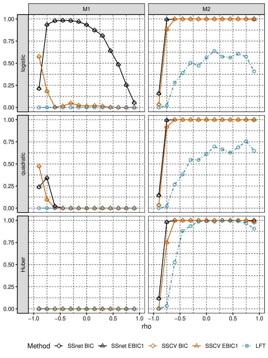
Figure 1: $P_{inc}$ for models M1 and M2

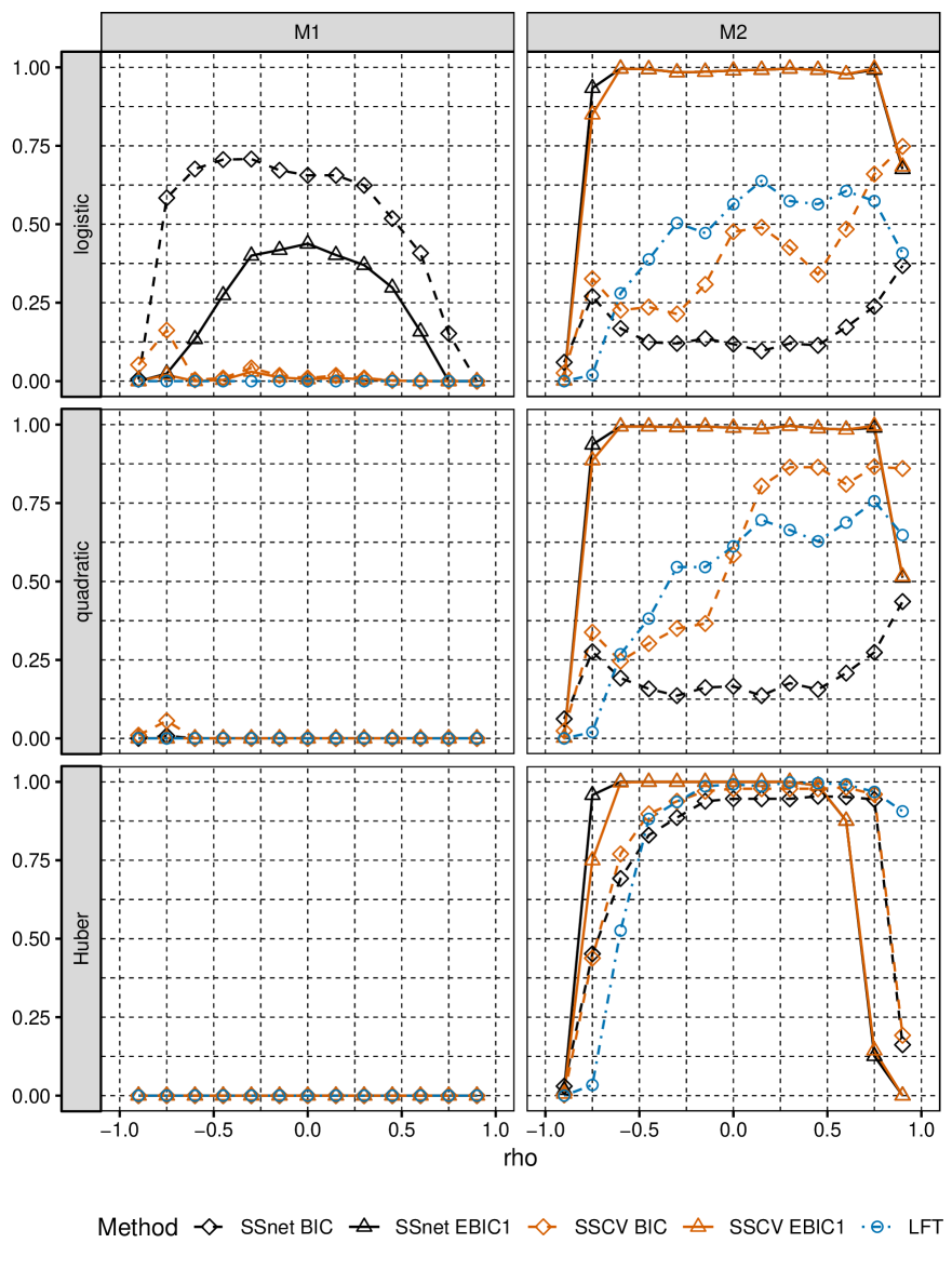
Figure 2: $P_{equal}$ for models M1 and M2

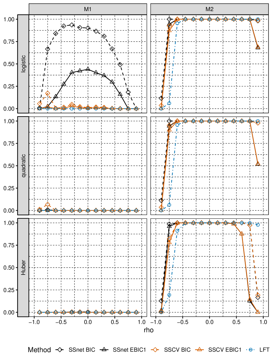
Figure 3: $P_{supset}$ for models M1 and M2

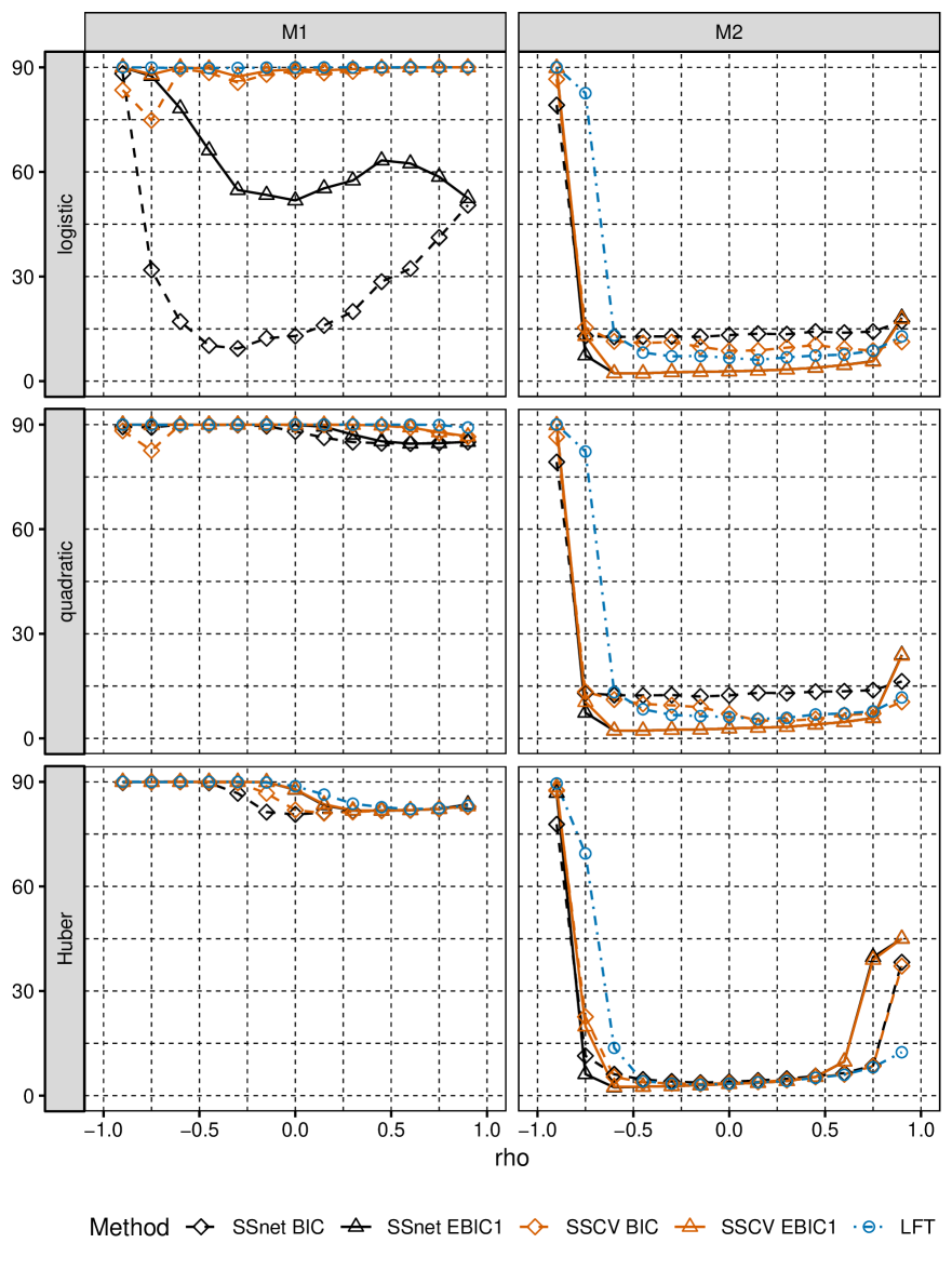
Figure 4: $ANGLE$ for models M1 and M2

7 Appendix

Proof of Lemma 1:

Proof.

Firstly, observe that function $R_{n}$ is convex as $\rho$ is convex. Moreover, from the definition of $\hat{\beta}_{L}$ we get the inequality:

$$W_{n}(\hat{\beta}_{L})=R_{n}(\hat{\beta}_{L})-R_{n}(\beta^{*})\leq\lambda(||\beta^{*}||_{1}-||\hat{\beta}_{L}||_{1}).$$ (32)

We note that $v-\beta^{*}\in B_{1}(r),$ as we have:

$$||v-\beta^{*}||_{1}=\frac{||\hat{\beta}_{L}-\beta^{*}||_{1}}{r+||\hat{\beta}_{L}-\beta^{*}||_{1}}\cdot r\leq r.$$ (33)

By definition of $W_{n},$ convexity of $R_{n}$, (33) and definition of $S$ we have:

$$W(v) =W(v)-W_{n}(v)+R_{n}(v)-R_{n}(\beta^{*})$$

$$\leq W(v)-W_{n}(v)+u(R_{n}(\hat{\beta}_{L})-R_{n}(\beta^{*}))\leq S(r)+uW_{n}(\hat{\beta}_{L}).$$ (34)

From the convexity of $l_{1}$ norm, (34), (32), $||\beta^{*}||_{1}=||\beta^{*}_{s^{*}}||_{1}$ and triangle inequality it follows that:

$$W(v)+\lambda||v||_{1} \leq W(v)+\lambda u||\hat{\beta}_{L}||_{1}+\lambda(1-u)||\beta^{*}||_{1}$$

$$\leq S(r)+uW_{n}(\hat{\beta}_{L})+u\lambda(||\hat{\beta}_{L}||_{1}-||\beta^{*}||_{1})+\lambda||\beta^{*}||_{1}$$

$$\leq S(r)+\lambda||\beta^{*}||_{1}\leq S(r)+\lambda||\beta^{*}-v_{s^{*}}||_{1}+\lambda||v_{s^{*}}||_{1}.$$ (35)

Hence:

$$W(v)+\lambda||v-\beta^{*}||_{1}=(W(v)+\lambda||v||_{1})+\lambda(||v-\beta^{*}||_{1}-||v||_{1})\\ \leq S(r)+\lambda||\beta^{*}-v_{s^{*}}||_{1}+\lambda||v_{s^{*}}||_{1}+\lambda(||v-\beta^{*}||_{1}-||v||_{1})=S(r)+2\lambda||\beta^{*}-v_{s^{*}}||_{1}.$$

∎

Lemma 4.

Assume that $S\sim Subg(\sigma^{2})$ and $T$ is random variable such that $|T|\leq M,$ where $M$ is some positive constant and $S$ and $T$ are independent. Then $ST\sim Subg(M^{2}\sigma^{2}).$

Proof.

Observe that:

$$Ee^{tST}=E(E(e^{tST}|T))\leq Ee^{\frac{t^{2}T^{2}\sigma^{2}}{2}}\leq e^{\frac{t^{2}M^{2}\sigma^{2}}{2}}.$$

∎

References

- Bach (2010) F. Bach. Self-concordant analysis for logistic regression. Electronic Journal of Statistics, 4:384–414, 2010.
- Bickel et al. (2009) P. Bickel, Y. Ritov, and A. Tsybakov. Simultaneous analysis of Lasso and Dantzig selector. Annals of Statistics, 37:1705–1732, 2009.
- Brillinger (1982) D. Brillinger. A generalized linear model with ’gaussian’ regressor variables. Festschfrift for Erich Lehmann, pages 97–113, 1982.
- Bühlmann and van de Geer (2011) P. Bühlmann and S. van de Geer. Statistics for High-dimensional Data. Springer, New York, 2011.
- Chen and Chen (2008) J. Chen and Z. Chen. Extended bayesian information criterion for model selection with large model spaces. Biometrika, 95:759–771, 2008.
- Chen and Chen (2012) J. Chen and Z. Chen. Extended BIC for small-n-large-p sparse glm. Statistica Sinica, 22:555–574, 2012.
- Devroye and Lugosi (2012) L. Devroye and G. Lugosi. Combinatorial Methods in Density Estimation. Springer Science & Business Media, 2012.
- Fan et al. (2014a) J. Fan, L Xue, and H. Zou. Strong oracle optimality of folded concave penalized estimation. Annals of Statistics, 43:819–849, 2014a.
- Fan et al. (2014b) J Fan, L Xue, and H Zou. Supplement to “Strong oracle optimality of folded concave penalized estimation.”, 2014b.
- Fan and Tang (2013) Y. Fan and C. Tang. Tuning parameter selection in high dimensional penalized likelihood. Journal of the Royal Statistical Society: Series B (Statistical Methodology), 75(3):531–552, 2013.
- Friedman et al. (2010) J. Friedman, T. Hastie, and R. Tibshirani. Regularization paths for generalized linear models via coordinate descent. Journal of Statistical Software, 33(1):1–22, 2010.
- Hastie et al. (2015) T. Hastie, R. Tibshirani, and M. Wainwright. Statistical Learning with Sparsity. Springer, New York, 2015.
- Huang et al. (2008) J. Huang, S. Ma, and C.H. Zhang. Adaptive Lasso for sparse high-dimensional regression models. Statistica Sinica, 18:1603–1618, 2008.
- Kim and Jeon (2016) Y. Kim and J-J. Jeon. Consistent model selection criteria for quadratically supported risks. The Annals of Statistics, 44(6):2467–2496, 2016.
- Kubkowski and Mielniczuk (2017) M. Kubkowski and J. Mielniczuk. Active set of predictors for misspecified logistic regression. Statistics, 51:1023–1045, 2017.
- Kubkowski and Mielniczuk (2018) M. Kubkowski and J. Mielniczuk. Projections of a general binary model on logistic regrssion. Linear Algebra and Applications, 536:152–173, 2018.
- Ledoux and Talagrand (1991) M. Ledoux and M. Talagrand. Probability in Banach Spaces: Isoperimetry and Processes. Springer, 1991.
- Li and Duan (1989) K.C. Li and N. Duan. Regression analysis under link violation. Annals of Statistics, 17:1009–1052, 1989.
- Lu et al. (2012) W. Lu, Y. Goldberg, and J. Fine. On the robustness of the adaptive laasso to model misspecification. Biometrika, 99:717–731, 2012.
- Mielniczuk and Szymanowski (2015) J. Mielniczuk and H. Szymanowski. Selection consistency of Generalized Information Criterion for sparse logistic model. Stochastic Models, Statistics and their Applications, pages 111–118, 2015.
- Negahban et al. (2012) Sahand N Negahban, Pradeep Ravikumar, Martin J Wainwright, and Bin Yu. A unified framework for high-dimensional analysis of -estimators with decomposable regularizers. Statistical Science, 27(4):538–557, 2012.
- Pokarowski and Mielniczuk (2015) P. Pokarowski and J. Mielniczuk. Combined and greedy penalized least squares for linear model selection. Journal of Machine Learning Research, 16(5):961–992, 2015.
- Pokarowski et al. (2018) P. Pokarowski, A. Prochenka, M. Frej, W. Rejchel, and J. Mielniczuk. Improving lasso for model selection and prediction. Unpublished manuscript, 2018. available from: https://www.univie.ac.at/seam/inference2018/abstracts/contributed/rejchel.pdf.
- Rosset et al. (2004) S. Rosset, J. Zhu, and T. Hastie. Boosting as a regularized path to a maximum margin classifier. Journal of Machine Learning Research, 5(Aug):941–973, 2004.
- Ruud (1983) P. Ruud. Suffcient conditions for the consistency of maximum likelihood estimation despite misspecifcation of distribution in multinomial discrete choice models. Econometrica, 51:225–228, 1983.
- Tibshirani (2013) R. Tibshirani. The lasso problem and uniqueness. Electronic Journal of Statistics, 7:1456–1490, 2013.
- van der Vaart and Wellner (1996) Aad W. van der Vaart and Jon A. Wellner. Weak Convergence and Empirical Processes with Applications to Statistics. Springer, 1996.
- Vuong (1989) Q. Vuong. Likelihood ratio testts for model selection and not-nested hypotheses. Econometrica, 57(2):307–333, 1989.
- White (1982) W. White. Maximum likelihood estimation of misspecified models. Econometrica, 50(3):1–25, 1982.
- Yi and Huang (2017) C. Yi and J. Huang. Semismooth Newton coordinate descent algorithm for elastic-net penalized Huber loss regression and quantile regression. Journal of Computational and Graphical Statistics, 26(3):547–557, 2017. doi: 10.1080/10618600.2016.1256816. URL https://doi.org/10.1080/10618600.2016.1256816.
- Zhou (2010) S. Zhou. Thresholded Lasso for high dimensional variable selection and statistical estimation. 2010.