accelerated piston problem and high order MBTZhifang Du and Jiequan Li
Accelerated Piston Problem and High Order Moving Boundary Tracking Method for Compressible Fluid Flows
Abstract
Reliable tracking of moving boundaries is important for the simulation of compressible fluid flows and there are a lot of contributions in literature. We recognize from the classical piston problem, a typical moving boundary problem in gas dynamics, that the acceleration is a key element in the description of the motion and it should be incorporated into the design of a moving boundary tracking (MBT) method. Technically, the resolution of the accelerated piston problem boils down to a one-sided generalized Riemann problem (GRP) solver, which is taken as the building block to construct schemes with the high order accuracy both in space and time. In this paper we take this into account, together with the cell-merging approach, to propose a new family of high order accurate moving boundary tracking methods and verify its performance through one- and two-dimensional test problems, along with accuracy analysis.
keywords:
Compressible fluid flows, accelerated piston problem, moving boundary tracking method, one-sided GRP solver, cell-merging criterion.35L50, 35L65, 65M08, 76M12, 76N15
1 Introduction
Moving boundary problems are ubiquitous for engineering applications and particularly the tracking of moving boundaries is an essential technique determining the quality of underlying simulations for compressible fluid flows. There are a lot of studies in this context, e.g., the front tracking method [15], the moving boundary tracking (MBT) method [11, 27], the immersed boundary method [23], level set methods [10], volume of fluid methods [14], moment of fluid methods [9], adaptive mesh refinement methods [6] and many others. In this paper, we will follow the moving boundary tracking method in the finite volume framework, with the new recognition of the key role of the acceleration in the description of moving boundaries, to develop a high order accurate version. Our study is motivated by a basic moving boundary problem, the accelerated piston problem in gas dynamics [7].
Assume that a uniform piston with a thickness , moves in a tube filled with gas. Its motion is described by two elements, the velocity and the acceleration [28],
| (1) |
where , and are the location, the velocity and the mass of the piston, is the sectional area of the tube and are pressures exerted on the two faces of the piston. The two equations in (1) are the Newtonian first and second laws for fluid flows, respectively, and they are coupled with the Euler equations, leading to a coupled dynamical system [18]. This might be the simplest moving (free) boundary problem in the context of compressible flows. It is natural to use the pair for the tracking of this piston, more or less like the symplectic algorithm [12],
| (2) |
where is the time increment. Otherwise, one would have to use the Runge-Kutta type time stepping to advance the trajectory of the piston, for which only the velocity is adopted. As the piston is resolved together with the evolution of the fluid flow in the whole flow region, the problem boils down to the one-sided generalized Riemann problem (GRP), the so-called initial boundary value problem (IBVP) with the piston as a free boundary. Numerically, when the finite volume framework is adopted, it is necessary to develop a one-sided GRP solver in order to construct numerical fluxes on the piston surface, and track the moving boundary (piston). The current study just establishes the interrelation between the resolution of the accelerated piston problem and the MBT method, leading to a high order version of MBT.
The moving boundary tracking method was originated in [11], and its advantage was clearly stated there. Since the uniformity of flow variables is assumed in boundary cells and the one-sided Riemann solver is adopted to compute the corresponding numerical fluxes, the MBT algorithm developed there has at most the first order accuracy in boundary cells [11, page 91]. The present contribution uses the direct Eulerian GRP solver [5], which enables us to develop a one-sided GRP solver suited for the MBT methodology to achieve the high order accuracy. The boundary can be tracked with high order accuracy simultaneously and no extra technology is needed. Besides, since the present GRP solver has been updated for multi-dimensional computations [21], the dimensional operator-splitting algorithm in [11] is not necessary. As far as complex geometries are concerned, the present paper adopts the cell-merging approach in [26, 25] to deal with the “small-cell” problem. Small cut cells are absorbed by their neighbors to form larger control volumes and fluid states are evolved over time-varying control volumes so that the resulting MBT scheme is consistent with the integrated form of conservation laws. This is different from the body-fitted or adaptive grid schemes [1, 22, 8, 24]. The MBT is also applied in other frameworks, e.g., the wave propagation algorithm [27]. We particularly refer to the inverse Lax-Wendroff (ILW) method [29], which interpolates the ghost fluid state with high-order spatial accuracy by taking the boundary acceleration into consideration. The temporal accuracy is obtained by the popular Runge-Kutta discretization.
This paper is organized as follows.
Basic facts about the rigid body motion and the MBT method are given in Section 2.
One- and two-dimensional one-sided GRP solvers are developed in Section 3.
The moving boundary tracking scheme is proposed in Section 4. The numerical accuracy of the newly developed MBT method is analyzed in Section 5.
Numerical experiments involving fluid-surface interactions are carried out in Section 6 for the performance. Some discussions are made in Section 7.
2 Accelerated piston problem and moving boundary tracking method
This section describes the piston problem, which motivates the new high-order MBT scheme that we are going to propose. The key observation is that the acceleration of a boundary should be taken as a natural and necessary element to describe its motion. Let’s describe the rigid body motion in one and two space dimensions.
2.1 Rigid body motion and accelerated piston problem
Think of a rigid body, represented by the polygon with its barycenter locating at , moving in the compressible fluid with a translational velocity and a rotational velocity , as shown in Figure 1. The rotational velocity is regarded as a pseudovector, which is positive if rotates counter-clockwise. The flow field around this body is described by the compressible Euler equations (only two-dimensional in the present paper, and similarly for three dimensional cases),
| (3) |
where is the velocity in the -coordinates, is the density, is the pressure, is the total energy. The internal energy is determined by the equation of state (EOS) . Thermodynamical quantities satisfy the Gibbs relation,
| (4) |
where and is the entropy. For polytropic gases, and is the specific heat ratio.

The boundary of the rigid body is denoted by with the unit normal vector pointing from the fluid to the rigid body. Then the motion of the body obeys
| (5) |
and its rotational motion is described using the equations
| (6) |
where is the mass of the solid body, and are the relative angle and the angular velocity of with respect to its barycenter , and is the inertia of the solid body. For , denote by its trajectory from for . The instantaneous translational motion of any point is described by
| (7) |
where , and are prescribed, is the velocity of the boundary point . We use the notation for any vector . Assume for the time being that the motion is not affected by surroundings in order to avoid the complications caused by the interaction with other boundaries. In order to describe the interaction between the rigid body and the compressible fluid, a proper boundary condition along the moving boundary is required,
| (8) |
where is the unit normal vector of at , pointing from the fluid into the rigid body.
When the problem reduces to one dimensional cases, the rigid body motion in the flow field corresponds to the free piston problem [7, 28], as described in Introduction. As far as the motion of the piston is concerned, we ignore the discussion on both ends of the cylinder and assume that this piston moves over the whole line. The thickness can be also assumed to be infinitely small. Then and are obtained by simultaneously solving the following two (left and right) free boundary problems,
| (9) |
and
| (10) |
where the velocity is defined through (1). Note that the pressure gradient determines the acceleration and the pressure exerted on the piston is not identical in general. Therefore, is not constant in and the piston is accelerated. This is called the accelerated piston problem. This observation will be put in the design of the high order MBT method in this paper.
2.2 Moving boundary tracking methods
The high order moving boundary tracking (MBT) method we are going to propose works in the finite volume framework, along with the cell-merging algorithm. Since the control volumes are Eulerian in the interior of the computational domain, we just focus on boundary control volumes. For easy understanding of the presentation, we first describe the one-dimensional version and then the two-dimensional case.
In one dimension, we consider the piston problem from the left and assume that the fluid occupied region is by ignoring the influence of the far field in the left. The computational domain is divided into uniform cells
| (11) |
We focus on the moving boundary (piston) cell. Assume that the piston is located in the rightmost cell indexed by , i.e. . Denote by the “legal” cell according to the following cell-merging criterion. Then we apply (3) over the space-time control volume ,
| (12) |
where and . The MBT method consists of three ingredients: the flow evolution, the boundary tracking and the cell merging. As usually implemented for the flow evolution, we need to approximate the fluxes properly. The interior flux is evaluated using the standard GRP solver [5]. However, the boundary flux depends on the one-sided GRP solver that provides the values
| (13) |
where is the directional derivative along the boundary . This pair of values also serves to track the boundary, as expressed in (2).
As the piston travels to the next time level , the boundary cell could be very small or large so that it should be redistributed, obeying a cell-merging criterion described below.
1-D Cell Merging Criterion (CMC)
-
a.
If and where is a user-tuned parameter, then is still well-defined. Otherwise, and are merged to form a new boundary cell, denoted as .
-
b.
If , the boundary control volume is .
-
c.
If , the boundary cell is .
In two dimensions, we still use the Cartesian meshes,
| (14) |
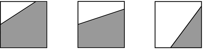
The Cartesian computational cells are usually cut by the boundary of solid objects to form very small “illegal” cells. We use the cell merging approach to modify boundary cells [25]. Generally, the shape of a cut cell may be a triangle, a quadrangle or a pentagon, as shown in Figure 2. For the time being, we assume is a “legal” boundary cell surrounded by the interior interface and the moving boundary . Denote by the space-time control volume. As the flow equations (3) are applied over this control volume, we obtain
| (15) |
where is the unit outer normal vector of . In parallel to the one-dimensional case, we develop 2-D one-sided GRP solver to provide the instantaneous values
| (16) |
where is any point on at , and . These values serve to approximate the flux and the track the moving boundary in the spirit of the GRP method.
The tracking of the moving boundary is much more involved, compared to the one-dimensional counterpart, and is described by (7). For the efficiency of algorithm, the cell-merging procedure is still necessary to avoid very small boundary cells.
The cell-merging procedure is stated briefly as follows. Suppose that the volume of is small enough, i.e., , is a user-tuned parameter. Then it should be absorbed by its neighbors to form a larger “legal” computational cell. Denote the normal vector at the segment by .
2-D Cell Merging Criterion (2D-CMC)
-
a.
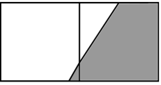
If is a triangle, combine it with its neighbor. For example, consider the situation shown in Figure 3(a), where , combine with . Otherwise, combine with .
-
b.
If is a quadrangle, combine it with its uncut neighbor. For example, consider the situation shown in Figure 3(b), combine with .
-
c.
Consider the situation that the cut cells are pentagons. Assume that a pentagon has two cut edges. Then there are two cases for the merging, depending on their lengths.
-
(i)
If one of its cut edges is too short, combine the pentagon with its neighbor to lengthen this cut edge, as shown in Figure 3(c).
-
(ii)
Otherwise, leave the pentagon as a “legal” cell.
-
(i)


3 One-sided generalized Riemann problem (OS-GRP) solver
In order to develop a high order moving boundary tracking scheme in the finite volume framework, we need to approximate the flux with a high order accuracy, which boils down to solving the following one-sided generalized Riemann problem (GRP). In this sense, the accelerated piston problem (9) is also called the one-sided generalized Riemann problem. Two cases are discussed: the 1-D one-sided GRP solver and the 2-D one-sided GRP solver. The difference between them is that the transversal effect relative to the boundary interface is incorporated in the 2-D GRP solver.
3.1 One-sided generalized Riemann problem solver in one dimension (OS-GRP-1D)
The one-sided GRP for the Euler equations in one space dimension is formulated as
| (17) |
where is a smooth vector function and usually taken as a polynomial for the numerical purpose. The boundary trajectory is defined following the dynamical system as
| (18) |
where the pair of the initial position and velocity of the piston is prescribed, and the pressures will be given later. Compared to (1), the thickness of the piston is assumed to be infinitely small and ignored.
Remark 3.1.
This one-sided generalized Riemann problem can be formulated from the right-hand side in the same way, thanks to the Galilean invariance.
Such a problem can be solved rigorously at least for a short time, following [28]. However, we are satisfied with the calculation of the instantaneous values
| (13) |
for the implementation of the high order moving boundary tracking method we propose. The same as the general GRP methodology [5], the calculation of (13) depends on solving the associated one-sided Riemann problem as formulated below.
Associated one-sided Riemann solver. In order to solve the above one-sided GRP (17), we firstly solve the one-sided Riemann problem following [7]. The associated one-sided Riemann problem is defined by approximating (17) with a constant initial data and neglecting the acceleration of the piston, which leads to the following IBVP
| (19) |
where is regarded as a constant state. The boundary condition in (19) says that the piston moves with a uniform velocity, which alludes to the fact that no force is exerted on the piston. This is very different from the GRP solver that exhibits the acceleration effect.
The one-sided Riemann solver follows from the standard Riemann solver, e.g. in [11], to obtain the one-sided Riemann solution , by noting that the velocity of the one-sided Riemann solution is
| (20) |
The pressure exerted on the piston is obtained through the standard analysis for the Riemann solver, as figuratively shown in Figure 4.


One-sided GRP solver (OS-GRP-1D). The one-sided GRP (17) is asymptotically consistent with the one-sided Riemann problem (19) in the sense that
| (21) |
Symmetrically, the one-sided GRP from the right-hand side, as formulated in (10), is associated with the right one-sided Rimann problem,
| (22) |
where the annotation of obvious notations is suppressed. Note that the pressures from both sides are different, generally speaking
| (23) |
So the piston is accelerated, according to (18),
| (24) |
This is the instantaneous acceleration of the piston for the one-sided GRP solver. Once we have this, we immediately use the standard GRP solver [5] to derive the relation
| (25) |
where , the coefficients , and are determined from , and , as usually done for the GRP solver [5]. The procedure to calculate coefficients in (25) exactly follows that given in [5]. Readers are referred there for details.
3.2 One-sided generalized Riemann problem solver in two dimensions (OS-GRP-2D)
Think of a solid body in two dimensions with the initial translational and rotational velocities and . The pressure exerted on the surface determines the acceleration. Our strategy is made as follows: At any point on the surface, we will first solve the one-sided Riemann problem normal to the surface to obtain the pressure, which yields the translational and rotational accelerations of the surface according to (5) and (6). Then we develop 2-D one-sided GRP solver to obtain the instantaneous value of the derivative for the flux evaluation and the boundary tracking.
Denote by the initial position of the solid surface and recall the notations in (7). For any , denote by the trajectory from for . The unit normal vector of at is denoted by and the instantaneous velocity of the solid surface at is denoted by .
One-sided normal Riemann solver. For the sake of presentation simplicity, we place the section of the moving boundary we concern initially along the -axis, thanks to the Galilean invariance. Define the associated one-sided normal Riemann problem at any point on the surface of the solid body as
| (27) |
where the superscript “” indicates the vector normal to the boundary . As far as the associated one-sided normal Riemann problem is concerned, the piston velocity in the IBVP (27) is defined as , where is given by the first equation in (7). The IBVP (27) can be solved exactly in the same way as the one-dimensional one-sided Riemann problem (19). The corresponding result of solving the above associated one-sided normal Riemann problem is denoted as .
One-sided GRP solver in 2-D. Once we know the total pressure on the surface using the one-sided normal Riemann solver, we can calculate the acceleration according to (5) and (6), the numerical discretizations of which will be specified in Subsection 4.2. Then we can solve the following two-dimensional one-sided generalized Riemann problem,
| (28) |
where, in light of (7), is the trajectory of the boundary point starting from and its velocity is . The 2-D GRP solver serves to obtain the instantaneous values at any point
| (29) |
for any and particularly , where is the directional derivative along the particle path. Remind again that is just the one-sided normal Riemann solution of (27), and is given as , which provides the local acceleration.
Different from the one-dimensional one-sided GRP solver, the transversal effect, as pointed out in [19], is important. Following [21], we regard the transversal term as a local source term and solve the following IBVP,
| (30) |
where is a fixed value, as described in [21]. Then the 2-D one-sided GRP solver for (28) is derived exactly the same as the 2-D GRP solver in [4, 21].
4 High-order moving boundary tracking algorithm
This section describes a high order moving boundary tracking algorithm based the newly developed one-sided GRP solver. This resulting scheme is different from those using the ghost fluid approach [17, 29], but can be regarded as the high order extension of MBT in [11].
4.1 One-dimensional high order MBT algorithm
The algorithm consists of three ingredients, as pointed out in Section 2: The evolution of flows, the moving boundary tracking and the boundary cell merging. The flow motion in the interior domain is treated using the standard finite volume method, e.g., the GRP method in [5]. So we focus on the boundary cell, which is denoted as . The algorithm is described as follows.
-
(i)
Implementation of one-sided GRP solver. Given the initial data over the boundary cell at ,
(31) we use the one-sided GRP solver to obtain the instantaneous values , which is annotated in (13). Then we compute the mid-point values for the flux approximation and interface values for slope evaluation at the next time level,
(32) -
(ii)
The tracking of the moving boundary. We track the moving boundary to the next time level using the formula within the second order accuracy,
(33) - (iii)
-
(iv)
Cell-merging procedure. Obey the 1-D cell-merging criterion to construct a “legal” boundary cell at the new time level .
-
(v)
Data update. Update the slope over the boundary cell ,
(36) where is a user defined parameter. Then we reconstruct the data in the form (31) over the boundary cell .
4.2 Two-dimensional high order MBT algorithm
The 2-D MBT algorithm has the same methodology as the 1-D case, in addition that the moving boundary tracking is more technical. Therefore we only provide details for boundary tracking and the data reconstruction, by assuming that all necessary values are available from the 2-D one-sided GRP solver. We still use the Cartesian mesh as expressed in (14). At , denote by the cells cut by for . Denote the segment of inside by with the middle point .
-
(i)
2-D moving boundary tracking. In light of (7), the instantaneous velocity at the middle point of is given by
(37) The associated one-sided normal Riemann problem (27) is consequently defined at . Denote the corresponding one-sided Riemann solution by . Particularly, the boundary pressure is obtained. Therefore the translational and rotational accelerations of are, according to (5) and (6),
(38) Consequently, in light of (7), the acceleration of the point is
(39) The above procedure of tracking the moving boundary provides the information of the piston motion required by the 2-D one-sided GRP solver to solve (30) in Section 3.2. At last, we update relevant values to the next time level as
(40) -
(ii)
Data reconstruction over boundary cells. For the cut cell , denote all of its edges by for . Furthermore, assume that . The unit outer normal vectors of with respect to are denoted by . In order to linearly approximate in , we need to estimate its gradient. By the Gauss theorem, we have
(41)
5 Accuracy analysis
In this section we check the accuracy of the proposed MBT method. We just focus on “legal” boundary cells . Recall the flux approximation in (35). Then we estimate
| (43) |
and
| (44) |
The flux difference yields,
| (45) |
It is evident that the time varying of boundary cells introduces extra errors. If the boundary is fixed, i.e., , we can achieve the second order accuracy for , which is written as
| (46) |
Otherwise the error has the form
| (47) |
which implies that if , the second order accuracy can be also achieved. By the way, if only the local one-sided Riemann solver is used [11], the accuracy reduces to first order. The numerical example below confirms such an observation.
We use the example proposed in [13] to verify the accuracy of the current MBT method, with the comparison with the original MBT just using the Riemann solver in [11]. This example describes a tube filled with gas initially
where and will be specified later. The left and right ends of the tube is closed by a fixed wall and a moving piston, respectively. Two cases are considered. The first case has a uniform piston velocity , while the second case has a varying piston velocity . Computations stop at and the piston is located at for both cases.
We check the numerical accuracy under the condition that the time increment is chosen to be
| (48) |
where is the maximum signal speed. The CFL number is taken to be . Since the entropy is uniform for both cases, it is chosen for the comparison. As shown in Table 1 for the first case and in Table 2 for the second, the current MBT with the acceleration element achieves desired accuracy of order.
| mesh | MBT with one-sided Riemann solver | MBT with one-sided GRP solver | ||||||
|---|---|---|---|---|---|---|---|---|
| size | errors | orders | errors | orders | errors | orders | errors | orders |
| 1/40 | 2.49e-5 | 4.39e-4 | 1.54e-5 | 8.48e-5 | ||||
| 1/80 | 4.11e-6 | 2.60 | 1.65e-4 | 1.41 | 1.82e-6 | 3.08 | 6.75e-6 | 3.65 |
| 1/160 | 7.34e-7 | 2.48 | 6.09e-5 | 1.44 | 2.06e-7 | 3.15 | 7.28e-7 | 3.21 |
| 1/320 | 1.44e-7 | 2.35 | 2.29e-5 | 1.41 | 2.21e-8 | 3.21 | 7.65e-8 | 3.25 |
| 1/640 | 3.09e-8 | 2.33 | 8.80e-6 | 1.38 | 2.37e-9 | 3.22 | 7.97e-9 | 3.26 |
| 1/1280 | 7.16e-9 | 2.21 | 3.47e-6 | 1.34 | 3.03e-10 | 2.97 | 1.01e-9 | 2.98 |
| mesh | MBT with one-sided Riemann solver | MBT with one-sided GRP solver | ||||||
|---|---|---|---|---|---|---|---|---|
| size | errors | orders | errors | orders | errors | orders | errors | orders |
| 1/40 | 4.21e-4 | 1.73e-3 | 8.77e-5 | 1.12e-3 | ||||
| 1/80 | 1.42e-4 | 1.57 | 1.28e-3 | 0.44 | 1.27e-5 | 2.79 | 1.73e-4 | 2.70 |
| 1/160 | 5.77e-5 | 1.30 | 9.71e-4 | 0.40 | 2.23e-6 | 2.51 | 1.80e-5 | 3.27 |
| 1/320 | 2.56e-5 | 1.17 | 7.56e-4 | 0.36 | 4.02e-7 | 2.47 | 3.08e-6 | 2.55 |
| 1/640 | 1.18e-5 | 1.12 | 6.03e-4 | 0.33 | 6.32e-8 | 2.67 | 5.97e-7 | 2.37 |
| 1/1280 | 5.48e-6 | 1.10 | 4.95e-4 | 0.29 | 8.52e-9 | 2.89 | 1.38e-7 | 2.11 |
6 Numerical experiments
In this section, we will present several typical examples to demonstrate the performance of the current MBT method. The first two examples are one-dimensional, while the last two are two-dimensional. These examples are already benchmark problems in this field, as referred accordingly. For all the four cases, the CFL number is taken to be .
6.1 Sudden motion of a piston with a rarefaction wave and a shock
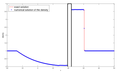
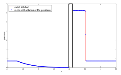
This benchmark test is taken from [27]. An infinitely long tube is filled with gas, initially having the state , and . A piston with the width is initially centered at . The piston suddenly moves to right with a constant speed , and then a shock forms ahead of the piston and a rarefaction wave behind the piston.
The computational domain is set to be , divided into equally distributed cells with the spatial size . The numerical results of the density and pressure are shown in Figure 5 and both of them match well with the exact solution.
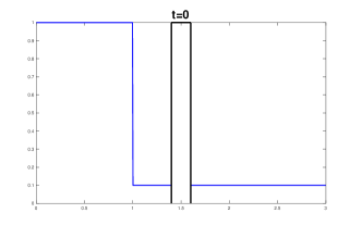
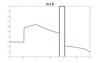
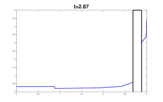
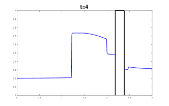
6.2 Sod shock interacting with a piston
We take this example from [16]. A tube occupies the space interval , filled with gas at rest initially,
Both ends of the tube are rigid walls. The computational domain is uniformly divided into cells. This tube is separated by a piston with the thickness , centered initially at . The motion of the piston passively depends on the force exerted from the fluid.
The fluid flow is described as follows: A shock from the left pushes the piston to the right. Since the right end of the tube is closed, the gas is compressed and the pressure increases as the piston moves right. Finally the piston is bounced back from the right.
Figure 6 shows the snapshots of the pressure of the flow field and the piston positions at different times , , , , respectively. The results matches well with those in [16].
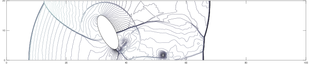
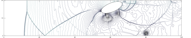
6.3 The kick off of 2-D objects
We consider an oval disk and a rectangular object interacting with a shock, respectively. A tunnel is units high, whose top and bottom boundaries are both reflective walls. Initially, a shock of Mach number is posed along and starts to move right. The pre-shock state of the gas is .
At first, consider an oval disk of the density , whose barycenter is placed at . The two axis of the oval disk are and units, respectively. The long axis of the oval disk is placed along the -axis. The mass of the disk is and the inertia of the disk is .
As the shock moves right, the disk would be kicked off from the ground, and rotates as it moves in the flow field.
The numerical computation is performed in the region divided by a grid.
Figure 7 shows the position of the disk and the pressure of the flow field at and , respectively. Multiple reflected shocks and vortices formed near the disk can be observed.
The numerical results match those proposed in [3] perfectly with better resolutions.
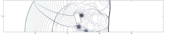
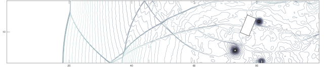
Now we replace the oval disk by a rectangular object whose barycenter initially locates at .
The long and short sides of the rectangle are and units, respectively.
The long side of the rectangle is posed at an angle of with the negative -direction. The mass and the inertia of the rectangle are and , where .
As the shock moves right, the rectangular object is kicked off. A computation is performed on a grid.
The positions of the rectangle and the pressure of the flow field are displayed in Figure 8, at and , respectively. Compared with the oval disk, a rectangular object has a larger inertia with respect to its size. Therefore it rotates less, as shown numerically. Besides, the cell-merging procedure is more involved.
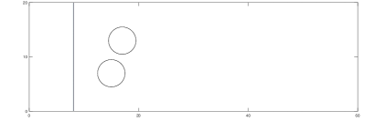
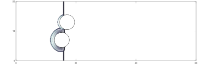
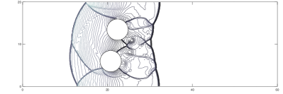
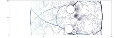
6.4 Two cylinders interacting with a shock
We simulate a more complicated problem with a shock interacting with two cylinders. Once again consider a tunnel units high whose top and bottom boundaries are both reflective walls. A Mach shock initially locates at . The pre-shock fluid state is . The two cylinders are positioned with barycenters at and , respectively. The radius and the density of the cylinders are and . A computation is carried out in the region with a grid. The pressure of the flow field and positions of two cylinders at , , and are displayed in Figure 9. It can be seen that the two cylinders are pushed away by the higher pressure between them.
7 Discussions
In this paper we observe from the classical piston problem in gas dynamics that the acceleration is an important element in the description of moving boundaries, and develop a one-sided GRP solver to design a high order moving boundary tracking algorithm, extending the MBT scheme originally developed in [11]. As analyzed, the newly developed MBT scheme is of second-order, and exhibits the desired performance.
As concluding remarks, we would like to make the following discussions.
-
(i)
It is a natural choice to use the pair , the velocity and the acceleration, to describe the motion of moving boundaries. In literature, this observation is not directly integrated into the design of high order schemes, possibly due to the absence of the one-sided GRP solver. Of course, this solver can be equivalently derived as in the context of gas kinetic scheme [30] or approximated, e.g., in [29], with applications in other framework such as the adaptive grid method [22, 1] and the over-lapping grid method [8, 24].
- (ii)
-
(iii)
The present paper just studies the moving boundary tracking of solid bodies. Careful check of the methodology stated in Section 2 indicates that this method can be extended to track various types of moving boundaries, e.g., in the context of multi-material flows and viscous flows etc. The key ingredient is how to evaluate the force exerted on the moving surface to compute out the acceleration.
References
- [1] N. Barral, G. Olivier, and F. Alauzet, Time-accurate anisotropic mesh adaptation for three-dimensional time-dependent problems with body-fitted moving geometries, J. Comput. Phys., 331 (2017), pp. 157–187.
- [2] T. J. Barth, Numerical methods for gasdynamic systems on unstructured meshes, in An Introduction to Recent Development in Theory and Numerics for Conservation Laws, D. Kröner, M. Ohlberger, and C. Rohde, eds., Springer-Verlag, Heidelberg, 1999, pp. 195–285.
- [3] M. Ben-Artzi and J. Falcovitz, Generalized Riemann Problems in Computational Fluid Dynamics, Cambridge University Press, Cambridge, 2003.
- [4] M. Ben-Artzi and J. Li, Hyperbolic balance laws: Riemann invariants and the generalized Riemann problem, Numer. Math., 106 (2007), pp. 369–425.
- [5] M. Ben-Artzi, J. Li, and G. Warnecke, A direct Eulerian GRP scheme for compressible fluid flows, J. Comput. Phys., 218 (2006), pp. 19–43.
- [6] M. Berger and P. Colella, Local adaptive mesh refinement for shock hydrodynamics, J. Comput. Phys., 82 (1989), pp. 64–84.
- [7] R. Courant and K. O. Friedrichs, Supersonic Flow and Shock Waves, Springer, New York, 1948.
- [8] F. C. Dougherty, J. A. Benek, and J. L. Steger, On applications of chimera grid schemes to store separation, tech. rep., National Aeronautics and Space Adnimistration, Moffett Field, California, 1985.
- [9] V. Dyadechko and M. Shashkov, Reconstruction of multi-material interfaces from moment data, J. Comput. Phys., 227 (2008), pp. 5361–5384.
- [10] R. F. F. Gibou and S. Osher, A review of level-set methods and some recent applications, J. Comput. Phys., 353 (2018), pp. 82–109.
- [11] J. Falcovitz, G. Alfandary, and G. Hanoch, A two-dimensional conservation laws scheme for compressible flow with moving boundaries, J. Comput. Phys., 138 (1997), pp. 83–102.
- [12] K. Feng and M. Qin, Symplectic Geometric Algorithms for Hamiltonian Systems, Springer, 2010.
- [13] H. Forrer and M. J. Berger, Flow simulations on Cartesian grids involving complex moving geometries, International Series of Numerical Mathematics, 129 (1999), pp. 315–324.
- [14] I. Ginzburg and G. Wittum, Two-phase flows on interface refined grids modeled with VOF, staggered finite volumes, and spline interpolants, J. Comput. Phys., 166 (2001), pp. 302–335.
- [15] J. Glimm, J. W. Grove, X. L. Li, and N. Zhao, Simple front tracking, Contemporary Mathematics, 238 (1999), pp. 133–149.
- [16] J. T. Gretarsson, N. Kwatra, and R. Fedkiw, Numerically stable fluid-structure interactions between compressible flow and solid structures, J. Comput. Phys., 230 (2011), pp. 3062–3084.
- [17] X. Y. Hu, B. C. Khoo, N. A. Adams, and F. L. Huang, A conservative interface method for compressible flows, J. Comput. Phys., 219 (2006), pp. 553–578.
- [18] E. Lefrançois and J.-P. Boufflet, An introduction to fluid-structure interaction: application to the piston problem, SIAM Review, 52 (2010), pp. 747–767.
- [19] X. Lei and J. Li, Transversal effects of high order numerical schemes for compressible fluid flows, Applied Mathematics and Mechanics (English Edition), 40 (2019), pp. 343–354.
- [20] J. Li, Two-stage fourth order: Temporal-spatial coupling in computational fluid dynamics (CFD), Advances in Aerodynamics, 1 (2019), pp. 1:3; 1–36.
- [21] J. Li and Z. Du, A two-stage fourth order time-accurate discretization for Lax-Wendroff type flow solvers, I. Hyperbolic conservation laws, SIAM J. Sci. Comput., 38 (2016), pp. A3046–A3069.
- [22] M. Olim, H. Nagoya, K. Takayama, and F. Hiatt, Entrainment of a dust particle by a flow behind a reflected shock wave, in the 19th International Symposium on Shock Waves, Universitéde Provence, Marseilles, France, July 1993, pp. 26–30.
- [23] C. S. Peskin, The immersed boundary method, Acta Numerica, 11 (2002), pp. 479–517.
- [24] L. Qiu, W. Lu, and R. Fedkiw, An adaptive discretization of compressible flow using a multitude of moving Cartesian grids, J. Comput. Phys., 305 (2016), pp. 75–110.
- [25] J. J. Quirk, An alternative to unstructured grids for computing gas dynamic flows around arbitrarily complex two-dimensional bodies, Comput. & Fluids, 23 (1994), pp. 125–142.
- [26] L. Schneiders, D. Hartmann, M. Meinke, and W. Schröder, An accurate moving boundary formulation in cut-cell methods, J. Comput. Phys., 235 (2013), pp. 786–809.
- [27] K.-M. Shyue, A moving-boundary tracking algorithm for inviscid compressible flow, in Hyperbolic Problems: Theory, Numerics, Applications, S. Benzoni-Gavage and D. Serre, eds., Springer, Berlin, Heidelberg, 2008, pp. 989–996.
- [28] S. Takeno, Free piston problem for isentropic gas dynamics, Japan J. Indust. Appl. Math., 12 (1995), pp. 163–194.
- [29] S. Tan and C.-W. Shu, A high order moving boundary treatment for compressible inviscid flows, J. Comput. Phys., 230 (2011), pp. 6023–6036.
- [30] K. Xu, A gas-kinetic BGK scheme for the Navier-Stokes equations and its connection with artificial dissipation and Godunov method, J. Comput. Phys., 171 (2001), pp. 289–335.