Inference and Uncertainty Quantification for
Noisy Matrix Completion

Abstract

Noisy matrix completion aims at estimating a low-rank matrix given only partial and corrupted entries. Despite substantial progress in designing efficient estimation algorithms, it remains largely unclear how to assess the uncertainty of the obtained estimates and how to perform statistical inference on the unknown matrix (e.g. constructing a valid and short confidence interval for an unseen entry).

This paper takes a step towards inference and uncertainty quantification for noisy matrix completion. We develop a simple procedure to compensate for the bias of the widely used convex and nonconvex estimators. The resulting de-biased estimators admit nearly precise non-asymptotic distributional characterizations, which in turn enable optimal construction of confidence intervals / regions for, say, the missing entries and the low-rank factors. Our inferential procedures do not rely on sample splitting, thus avoiding unnecessary loss of data efficiency. As a byproduct, we obtain a sharp characterization of the estimation accuracy of our de-biased estimators, which, to the best of our knowledge, are the first tractable algorithms that provably achieve full statistical efficiency (including the preconstant). The analysis herein is built upon the intimate link between convex and nonconvex optimization — an appealing feature recently discovered by [CCF⁺19].

Keywords: matrix completion, statistical inference, confidence intervals, uncertainty quantification, convex relaxation, nonconvex optimization

1 Introduction

1.1 Motivation: inference and uncertainty quantification?

Low-rank matrix completion is concerned with recovering a low-rank matrix, when only a small fraction of its entries are revealed to us [Sre04, CR09, KMO10a]. Tackling this problem in large-scale applications is computationally challenging, due to the intrinsic nonconvexity incurred by the low-rank structure. To further complicate matters, another inevitable challenge stems from the imperfectness of data acquisition mechanisms, wherein the acquired samples are contaminated by a certain amount of noise.

Fortunately, if the entries of the unknown matrix are sufficiently de-localized and randomly revealed, this problem may not be as hard as it seems. Substantial progress has been made over the past several years in designing computationally tractable algorithms — including both convex and nonconvex approaches — that allow to fill in unseen entries faithfully given only partial noisy samples [CP10, NW12, KLT11, KMO10b, CW15, MWCC17, CCF⁺19]. Nevertheless, modern decision making would often require one step further. It not merely anticipates a faithful estimate, but also seeks to quantify the uncertainty or “confidence” of the provided estimate, ideally in a reasonably accurate fashion. For instance, given an estimate returned by the convex approach, how to use it to compute a short interval that is likely to contain a missing entry?

Conducting effective uncertainty quantification for noisy matrix completion is, however, far from straightforward. For the most part, the state-of-the-art matrix completion algorithms require solving highly complex optimization problems, which often do not admit closed-form solutions. Of necessity, it is generally very challenging to pin down the distributions of the estimates returned by these algorithms. The lack of distributional characterizations presents a major roadblock to performing valid, yet efficient, statistical inference on the unknown matrix of interest.

It is worth noting that a number of recent papers have been dedicated to inference and uncertainty quantification for various high-dimensional problems in high-dimensional statistics, including Lasso [ZZ14, vdGBRD14, JM14a], generalized linear models [vdGBRD14, NL17, BFL⁺18], graphical models [JVDG15, RSZZ15, MLL17]), amongst others. Very little work, however, has looked into noisy matrix completion along this direction. While non-asymptotic statistical guarantees for noisy matrix completion have been derived in prior theory, most, if not all, of the estimation error bounds are supplied only at an order-wise level. Such order-wise error bounds either lose a significant factor relative to the optimal guarantees, or come with an unspecified (but often enormous) pre-constant. Viewed in this light, a confidence region constructed directly based on such results is bound to be overly conservative, resulting in substantial over-coverage.

1.2 A glimpse of our contributions

This paper takes a substantial step towards efficient inference and uncertainty quantification for noisy matrix completion. Specifically, we develop a simple procedure to compensate for the bias of the commonly used convex and nonconvex estimators. The resulting de-biased estimators admit nearly accurate non-asymptotic distributional guarantees. Such distributional characterizations in turn allow us to reason about the uncertainty of the obtained estimates vis-à-vis the unknown matrix. While details of our main findings are postponed to Section 3, we would like to immediately single out a few important merits of the proposed inferential procedures and theory:

1. Our results enable two types of uncertainty assessment, namely, we can construct (i) confidence intervals for each entry — either observed or missing — of the unknown matrix; (ii) confidence regions for the low-rank factors of interest (modulo some unavoidable global ambiguity).

2. Despite the complicated statistical dependency, our procedure and theory do not rely on sample splitting, thus avoiding the unnecessary widening of confidence intervals / regions due to insufficient data usage.

3. The confidence intervals / regions constructed based on the proposed procedures are, in some sense, optimal.

4. We present a unified approach that accommodates both convex and nonconvex estimators seamlessly.

5. As a byproduct, we characterize the Euclidean estimation errors of the proposed de-biased estimators. Such error bounds are sharp and match an oracle lower bound precisely (including the pre-constant). To the best of our knowledge, this is the first theory that demonstrates that a computationally feasible algorithm can achieve the statistical limit including the pre-constant.

All of this is built upon the intimate link between convex and nonconvex estimators [CCF⁺19], as well as the recent advances in analyzing the stability of nonconvex optimization against random noise [MWCC17].

2 Models and notation

To cast the noisy matrix completion problem in concrete statistical settings, we adopt a model commonly studied in the literature [CR09]. We also introduce some useful notation.

Ground truth.

Denote by $\bm{M}^{\star}\in\mathbb{R}^{n\times n}$ the unknown rank-$r$ matrix of interest, whose (compact) singular value decomposition (SVD) is given by $\bm{M}^{\star}=\bm{U}^{\star}\bm{\Sigma}^{\star}\bm{V}^{\star\top}$. We set

$$\sigma_{\max}\triangleq\sigma_{1}(\bm{M}^{\star}),\quad\sigma_{\min}\triangleq\sigma_{r}(\bm{M}^{\star}),\quad\text{and}\quad\kappa\triangleq\sigma_{\max}/\sigma_{\min},$$ (2.1)

where $\sigma_{i}(\bm{A})$ denotes the $i$th largest singular value of a matrix $\bm{A}$. Further, we let $\bm{X}^{\star}\triangleq\bm{U}^{\star}\bm{\Sigma}^{\star 1/2}\in\mathbb{R}^{n\times r}$ and $\bm{Y}^{\star}\triangleq\bm{V}^{\star}\bm{\Sigma}^{\star 1/2}\in\mathbb{R}^{n\times r}$ stand for the balanced low-rank factors of $\bm{M}^{\star}$, which obey

$$\bm{X}^{\star\top}\bm{X}^{\star}=\bm{Y}^{\star\top}\bm{Y}^{\star}=\bm{\Sigma}^{\star}\qquad\text{and}\qquad\bm{M}^{\star}=\bm{X}^{\star}\bm{Y}^{\star\top}.$$ (2.2)

Observation models.

What we observe is a random subset of noisy entries of $\bm{M}^{\star}$; more specifically, we observe

$$M_{ij}=M_{ij}^{\star}+E_{ij},\qquad E_{ij}\overset{\mathrm{i.i.d.}}{\sim}\mathcal{N}(0,\sigma^{2}),\qquad\text{for all }(i,j)\in\Omega,$$ (2.3)

where $\Omega\subseteq\{1,\cdots,n\}\times\{1,\cdots,n\}$ is a subset of indices, and $E_{ij}$ denotes independently generated noise at the location $(i,j)$. From now on, we assume the random sampling model where each index $(i,j)$ is included in $\Omega$ independently with probability $p$ (i.e. data are missing uniformly at random). We shall use $\mathcal{P}_{\Omega}(\cdot):\mathbb{R}^{n\times n}\mapsto\mathbb{R}^{n\times n}$ to represent the orthogonal projection onto the subspace of matrices that vanish outside the index set $\Omega$.

Incoherence conditions.

Clearly, not all matrices can be reliably estimated from a highly incomplete set of measurements. To address this issue, we impose a standard incoherence condition [CR09, Che15] on the singular subspaces of $\bm{M}^{\star}$ (i.e. $\bm{U}^{\star}$ and $\bm{V}^{\star}$):

$$\max\{\left\|\bm{U}^{\star}\right\|_{2,\infty},\left\|\bm{V}^{\star}\right\|_{2,\infty}\}\leq\sqrt{\mu r/n},$$ (2.4)

where $\mu$ is termed the incoherence parameter and $\|\bm{A}\|_{2,\infty}$ denotes the largest $\ell_{2}$ norm of all rows in $\bm{A}$. A small $\mu$ implies that the energy of $\bm{U}^{\star}$ and $\bm{V}^{\star}$ are reasonably spread out across all of their rows.

Asymptotic notation.

Here, $f(n)\lesssim h(n)$ (or $f(n)=O(h(n))$) means $|f(n)|\leq c_{1}|h(n)|$ for some constant $c_{1}>0$, $f(n)\gtrsim h(n)$ means $|f(n)|\geq c_{2}|h(n)|$ for some constant $c_{2}>0$, $f(n)\asymp h(n)$ means $c_{2}|h(n)|\leq|f(n)|\leq c_{1}|h(n)|$ for some constants $c_{1},c_{2}>0$, and $f(n)=o(h(n))$ means $\lim_{n\rightarrow\infty}f(n)/h(n)=0$. We write $f(n)\ll h(n)$ to indicate that $|f(n)|\leq c_{1}|h(n)|$ for some small constant $c_{1}>0$ (much smaller than 1), and use $f(n)\gg h(n)$ to indicate that $|f(n)|\geq c_{2}|h(n)|$ for some large constant $c_{2}>0$ (much larger than 1).

3 Inferential procedures and main results

The proposed inferential procedure lays its basis on two of the most popular estimation paradigms — convex relaxation and nonconvex optimization — designed for noisy matrix completion. Recognizing the complicated bias of these two highly nonlinear estimators, we shall first illustrate how to perform bias correction, followed by a distributional theory that establishes the near-Gaussianity and optimality of the proposed de-biased estimators.

3.1 Background: convex and nonconvex estimators

We first review in passing two tractable estimation algorithms that are arguably the most widely used in practice. They serve as the starting point for us to design inferential procedures for noisy low-rank matrix completion. The readers familiar with this literature can proceed directly to Section 3.2.

Convex relaxation.

Recall that the rank function $\mathsf{rank}(\cdot)$ is highly nonconvex, which often prevents us from computing a rank-constrained estimator in polynomial time. For the sake of computational feasibility, prior works suggest relaxing the rank function into its convex surrogate [Faz02, RFP10]; for example, one can consider the following penalized least-squares convex program

$$\underset{\bm{Z}\in\mathbb{R}^{n\times n}}{\textsf{minimize}}\qquad\frac{1}{2}\sum_{(i,j)\in\Omega}\left(Z_{ij}-M_{ij}\right)^{2}+\lambda\|\bm{Z}\|_{*},$$ (3.1)

or using our notation $\mathcal{P}_{\Omega}$,

$$\underset{\bm{Z}\in\mathbb{R}^{n\times n}}{\textsf{minimize}}\qquad\frac{1}{2}\big{\|}\mathcal{P}_{\Omega}\big{(}\bm{Z}-\bm{M}\big{)}\big{\|}_{\mathrm{F}}^{2}+\lambda\|\bm{Z}\|_{*}.$$ (3.2)

Here, $\|\cdot\|_{*}$ is the nuclear norm (the sum of singular values, which is a convex surrogate of the rank function), and $\lambda>0$ is some regularization parameter. Under mild conditions, the solution to the convex program (3.1) provably attains near-optimal estimation accuracy (in an order-wise sense), provided that a proper regularization parameter $\lambda$ is adopted [CCF⁺19].

Algorithm 1 Gradient descent for solving the nonconvex problem (3.4).

  Suitable initialization: $\bm{X}^{0}$, $\bm{Y}^{0}$

  Gradient updates: for $t=0,1,\ldots,t_{0}-1$ do

  

$$\bm{X}^{t+1}= \bm{X}^{t}-\frac{\eta}{p}\big{[}\mathcal{P}_{\Omega}(\bm{X}^{t}\bm{Y}^{t\top}-\bm{M})\bm{Y}^{t}+\lambda\bm{X}^{t}\big{]},$$ (3.3a)

$$\bm{Y}^{t+1}= \bm{Y}^{t}-\frac{\eta}{p}\big{[}[\mathcal{P}_{\Omega}(\bm{X}^{t}\bm{Y}^{t\top}-\bm{M})]^{\top}\bm{X}^{t}+\lambda\bm{Y}^{t}\big{]},$$ (3.3b)

where $$\eta>0$$ determines the step size or the learning rate.

Nonconvex optimization.

It is recognized that the convex approach, which typically relies on solving a semidefinite program, is still computationally expensive and not scalable to large dimensions. This motivates an alternative route, which represents the matrix variable via two low-rank factors $\bm{X},\bm{Y}\in\mathbb{R}^{n\times r}$ and attempts solving the following nonconvex program directly

$$\underset{\bm{X},\bm{Y}\in\mathbb{R}^{n\times r}}{\textsf{minimize}}\qquad\frac{1}{2}\big{\|}\mathcal{P}_{\Omega}\big{(}\bm{X}\bm{Y}^{\top}-\bm{M}\big{)}\big{\|}_{\mathrm{F}}^{2}+\frac{\lambda}{2}\|\bm{X}\|_{\mathrm{F}}^{2}+\frac{\lambda}{2}\|\bm{Y}\|_{\mathrm{F}}^{2}.$$ (3.4)

Here, we choose a regularizer of the form $0.5\lambda(\|\bm{X}\|_{\mathrm{F}}^{2}+\|\bm{Y}\|_{\mathrm{F}}^{2})$ primarily to mimic the nuclear norm $\lambda\|\bm{Z}\|_{*}$ (see [SS05, MHT10]). A variety of optimization algorithms have been proposed to tackle the nonconvex program (3.4) or its variants [SL16, CW15, MWCC17]; the readers are referred to [CLC19] for a recent overview. As a prominent example, a two-stage algorithm — gradient descent following suitable initialization — provably enjoys fast convergence and order-wise optimal statistical guarantees for a wide range of scenarios [MWCC17, CCF⁺19, CLL19]. The current paper focuses on this simple yet powerful algorithm, as documented in Algorithm 1 and detailed in Appendix A.1.

Intimate connections between convex and nonconvex estimates.

Denote by $\bm{Z}^{\mathsf{cvx}}$ any minimizer of the convex program (3.1), and denote by $(\bm{X}^{\mathsf{ncvx}},\bm{Y}^{\mathsf{ncvx}})$ the estimate returned by Algorithm 1 aimed at solving (3.4). As was recently shown in [CCF⁺19], when the regularization parameter $\lambda$ is properly chosen, these two estimates obey (see (A.12) in Appendix A.2 for a precise statement)

$$\bm{X}^{\mathsf{ncvx}}\bm{Y}^{\mathsf{ncvx}\top}\approx\bm{Z}^{\mathsf{cvx}}\approx\bm{Z}^{\mathsf{cvx},r}.$$ (3.5)

Here, $\bm{Z}^{\mathsf{cvx},r}\triangleq\mathcal{P}_{\text{rank-}r}(\bm{Z}^{\mathsf{cvx}})$ is the best rank-$r$ approximation of the convex estimate $\bm{Z}^{\mathsf{cvx}}$, where $\mathcal{P}_{\text{rank-}r}(\bm{B})\triangleq\arg\min_{\bm{A}:\text{rank}(\bm{A})\leq r}\|\bm{A}-\bm{B}\|_{\mathrm{F}}$. In truth, the three matrices of interest in (3.5) are exceedingly close to, if not identical with, each other. This salient feature paves the way for a unified treatment of convex and nonconvex approaches: most inferential procedures and guarantees developed for the nonconvex estimate can be readily transferred to perform inference for the convex one, and vice versa.

3.2 Constructing de-biased estimators

Table 1: Notation used to unify the convex estimate $\bm{Z}^{\mathsf{cvx}}$ and the nonconvex estimate $(\bm{X}^{\mathsf{ncvx}},\bm{Y}^{\mathsf{ncvx}})$. Here, $\bm{Z}^{\mathsf{cvx},r}=\mathcal{P}_{\text{rank-}r}(\bm{Z}^{\mathsf{cvx}})$ is the best rank-$r$ approximation of $\bm{Z}^{\mathsf{cvx}}$. See Appendix B for a complete summary.

$\bm{Z}\in\mathbb{R}^{n\times n}$	either $\bm{Z}^{\mathsf{cvx}}$ or $\bm{X}^{\mathsf{ncvx}}\bm{Y}^{\mathsf{ncvx}\top}$.
$\bm{X},\bm{Y}\in\mathbb{R}^{n\times r}$	for the nonconvex case, we take $\bm{X}=\bm{X}^{\mathsf{ncvx}}$ and $\bm{Y}=\bm{Y}^{\mathsf{ncvx}}$; for the convex case, let $\bm{X}=\bm{X}^{\mathsf{cvx}}$ and $\bm{Y}=\bm{Y}^{\mathsf{cvx}}$, which are the balanced low-rank factors of $\bm{Z}^{\mathsf{cvx},r}$ obeying $\bm{Z}^{\mathsf{cvx},r}=\bm{X}^{\mathsf{cvx}}\bm{Y}^{\mathsf{cvx}\top}$ and $\bm{X}^{\mathsf{cvx}\top}\bm{X}^{\mathsf{cvx}}=\vphantom{\frac{1}{2}}\bm{Y}^{\mathsf{cvx}\top}\bm{Y}^{\mathsf{cvx}}$.
$\bm{M}^{\mathsf{d}}\in\mathbb{R}^{n\times n}$	the proposed de-biased estimator as in (3.7).
$\bm{X}^{\mathsf{d}},\bm{Y}^{\mathsf{d}}\in\mathbb{R}^{n\times r}$	the proposed de-shrunken estimator as in (3.8).

We are now well equipped to describe how to construct new estimators based on the convex estimate $\bm{Z}^{\mathsf{cvx}}$ and the nonconvex estimate $(\bm{X}^{\mathsf{ncvx}},\bm{Y}^{\mathsf{ncvx}})$, so as to enable statistical inference. Motivated by the proximity of the convex and nonconvex estimates and for the sake of conciseness, we shall abuse notation by using the shorthand $\bm{Z},\bm{X},\bm{Y}$ for both convex and nonconvex estimates; see Table 1 and Appendix B for precise definitions. This allows us to unify the presentation for both convex and nonconvex estimators.

Given that both (3.1) and (3.4) are regularized least-squares problems, they behave effectively like shrinkage estimators, indicating that the provided estimates necessarily suffer from non-negligible bias. In order to enable desired statistical inference, it is natural to first correct the estimation bias.

A de-biased estimator for the matrix.

A natural de-biasing strategy that immediately comes to mind is the following simple linear transformation (recall the notation in Table 1):

$$\bm{Z}^{0}\triangleq\bm{Z}-\frac{1}{p}\mathcal{P}_{\Omega}\big{(}\bm{Z}-\bm{M}\big{)}=\underset{\text{mean:}\,\bm{M}^{\star}}{\underbrace{\frac{1}{p}\mathcal{P}_{\Omega}\big{(}\bm{M}^{\star}\big{)}}}+\underset{\text{mean:}\,\bm{0}}{\underbrace{\frac{1}{p}\mathcal{P}_{\Omega}\big{(}\bm{E}\big{)}}}+\underset{\text{mean:}\,\bm{0}\text{ (heuristically)}}{\underbrace{\bm{Z}-\frac{1}{p}\mathcal{P}_{\Omega}\big{(}\bm{Z}\big{)}}},$$ (3.6)

where we identify $\mathcal{P}_{\Omega}(\bm{M})$ with $\mathcal{P}_{\Omega}(\bm{M}^{\star})+\mathcal{P}_{\Omega}\left(\bm{E}\right)$. Heuristically, if $\Omega$ and $\bm{Z}$ are statistically independent, then $\bm{Z}^{0}$ serves as an unbiased estimator of $\bm{M}^{\star}$, i.e. $\mathbb{E}[\bm{Z}^{0}]=\bm{M}^{\star}$; this arises since the noise $\bm{E}$ has zero mean and $\mathbb{E}[\mathcal{P}_{\Omega}]=p\mathcal{I}$ under the uniform random sampling model, with $\mathcal{I}$ the identity operator. Despite its (near) unbiasedness nature at a heuristic level, however, the matrix $\bm{Z}^{0}$ is typically full-rank, with non-negligible energy spread across its entire spectrum. This results in dramatically increased variability in the estimate, which is undesirable for inferential purposes.

To remedy this issue, we propose to further project $\bm{Z}^{0}$ onto the set of rank-$r$ matrices, leading to the following de-biased estimator

$$\bm{M}^{\mathsf{d}}\triangleq\mathcal{P}_{\text{rank-}r}\Big{[}\bm{Z}-\frac{1}{p}\mathcal{P}_{\Omega}\left(\bm{Z}-\bm{M}\right)\Big{]},$$ (3.7)

where $\mathcal{P}_{\text{rank-}r}(\bm{B})=\arg\min_{\bm{A}:\text{rank}(\bm{A})\leq r}\|\bm{A}-\bm{B}\|_{\mathrm{F}}$, and $\bm{Z}$ can again be found in Table 1. This projection step effectively suppresses the variability outside the $r$-dimensional principal subspace. As we shall see shortly, the proposed estimator (3.7) properly de-biases the provided estimate $\bm{Z}$, while optimally controlling the extent of uncertainty.

Remark 1.

The estimator (3.7) can be viewed as performing one iteration of singular value projection (SVP)  [MJD09, DC18] on the current estimate $\bm{Z}$.

Remark 2.

The estimator (3.7) also bears a similarity to the de-biased estimator proposed by [Xia18] for low-rank trace regression; the disparity between them shall be discussed in Section 4.

An equivalent form: a de-shrunken estimator for the low-rank factors.

It turns out that the de-biased estimator (3.7) admits another almost equivalent representation that offers further insights. Specifically, we consider the following de-shrunken estimator for the low-rank factors

$$\bm{X}^{\mathrm{d}}\triangleq\bm{X}\Big{(}\bm{I}_{r}+\frac{\lambda}{p}\big{(}\bm{X}^{\top}\bm{X}\big{)}^{-1}\Big{)}^{1/2}\qquad\text{and}\qquad\bm{Y}^{\mathrm{d}}\triangleq\bm{Y}\Big{(}\bm{I}_{r}+\frac{\lambda}{p}\big{(}\bm{Y}^{\top}\bm{Y}\big{)}^{-1}\Big{)}^{1/2},$$ (3.8)

where we recall the definition of $\bm{X}$ and $\bm{Y}$ in Table 1. To develop some intuition regarding why this is called a de-shrunken estimator, let us look at a simple scenario where $\bm{U}\bm{\Sigma}\bm{V}^{\top}$ is the SVD of $\bm{X}\bm{Y}^{\top}$ and $\bm{X}=\bm{U}\bm{\Sigma}^{1/2}$, $\bm{Y}=\bm{V}\bm{\Sigma}^{1/2}$. It is then self-evident that

$$\bm{X}^{\mathsf{d}}=\bm{U}\bm{\Sigma}^{1/2}\Big{(}\bm{I}_{r}+\frac{\lambda}{p}\bm{\Sigma}^{-1}\Big{)}^{1/2}=\bm{U}\Big{(}\bm{\Sigma}+\frac{\lambda}{p}\bm{I}_{r}\Big{)}^{1/2}\qquad\text{and}\qquad\bm{Y}^{\mathsf{d}}=\bm{V}\Big{(}\bm{\Sigma}+\frac{\lambda}{p}\bm{I}_{r}\Big{)}^{1/2}.$$

In words, $\bm{X}^{\mathsf{d}}$ and $\bm{Y}^{\mathsf{d}}$ are obtained by de-shrinking the spectrum of $\bm{X}$ and $\bm{Y}$ properly.

As we shall formalize in Section 5.1, the de-shrunken estimator (3.8) for the low-rank factors is nearly equivalent to the de-biased estimator (3.7) for the whole matrix, in the sense that

$$\bm{M}^{\mathsf{d}}\approx\bm{X}^{\mathsf{d}}\bm{Y}^{\mathsf{d}\top}.$$ (3.9)

Therefore, $\bm{M}^{\mathrm{d}}$ can be viewed as some sort of de-shrunken estimator as well.

3.3 Main results: distributional guarantees

The proposed estimators admit tractable distributional characterizations in the large-$n$ regime, which facilitates the construction of confidence regions for many quantities of interest. In particular, this paper centers around two types of inferential problems:

1. Each entry of the matrix $\bm{M}^{\star}$: the entry can be either missing (i.e. predicting an unseen entry) or observed (i.e. de-noising an observed entry). For example, in the Netflix challenge, one would like to infer a user’s preference about any movie, given partially revealed ratings [CR09]. Mathematically, this seeks to determine the distribution of

   $$M_{ij}^{\mathrm{d}}-M_{ij}^{\star},\qquad\text{for all }1\leq i,j\leq n.$$ (3.10)

2. The low-rank factors $\bm{X}^{\star},\bm{Y}^{\star}\in\mathbb{R}^{n\times r}$: the low-rank factors often reveal critical information about the applications of interest (e.g. community memberships of each individual in the community detection problem [AFWZ17], or angles between each object and a global reference point in the angular synchronization problem [Sin11]). Recognizing the global rotational ambiguity issue, we aim to pin down the distributions of $\bm{X}^{\mathrm{d}}$ and $\bm{Y}^{\mathrm{d}}$ up to global rotational ambiguity. More precisely, we intend to characterize the distributions of

   $$\bm{X}^{\mathsf{d}}\bm{H}^{\mathsf{d}}-\bm{X}^{\star}\qquad\text{and}\qquad\bm{Y}^{\mathsf{d}}\bm{H}^{\mathsf{d}}-\bm{Y}^{\star}$$ (3.11)

   for the global rotation matrix $\bm{H}^{\mathsf{d}}\in\mathbb{R}^{r\times r}$ that best “aligns” $(\bm{X}^{\mathsf{d}},\bm{Y}^{\mathsf{d}})$ and $(\bm{X}^{\star},\bm{Y}^{\star})$, i.e.

   $$\bm{H}^{\mathsf{d}}\triangleq\arg\min_{\bm{R}\in\mathcal{O}^{r\times r}}\left\|\bm{X}^{\mathsf{d}}\bm{R}-\bm{X}^{\star}\right\|_{\mathrm{F}}^{2}+\left\|\bm{Y}^{\mathsf{d}}\bm{R}-\bm{Y}^{\star}\right\|_{\mathrm{F}}^{2}.$$ (3.12)

   Here and below, $\mathcal{O}^{r\times r}$ denotes the set of orthonormal matrices in $\mathbb{R}^{r\times r}$.

Clearly, the above two inferential problems are tightly related: an accurate distributional characterization for the low-rank factors (3.11) often results in a distributional guarantee for the entries (3.10). As such, we shall begin by presenting our distributional characterizations of the low-rank factors. Here and throughout, $\bm{e}_{i}$ represents the $i$th standard basis vector in $\mathbb{R}^{n}$.

Theorem 1 (Distributional guarantees w.r.t. low-rank factors).

Suppose that the sample size and the noise obey

$$np\gtrsim\kappa^{8}\mu^{3}r^{2}\log^{3}n\qquad\text{and}\qquad\sigma/\sigma_{\min}\lesssim\sqrt{p/(\kappa^{8}\mu n\log^{2}n)}.$$ (3.13)

Then one has the following decomposition

$$\bm{X}^{\mathsf{d}}\bm{H}^{\mathsf{d}}-\bm{X}^{\star} =\bm{Z}_{\bm{X}}+\bm{\Psi}_{\bm{X}},$$ (3.14a)

$$\bm{Y}^{\mathsf{d}}\bm{H}^{\mathsf{d}}-\bm{Y}^{\star} =\bm{Z}_{\bm{Y}}+\bm{\Psi}_{\bm{Y}}.$$ (3.14b)

with $(\bm{X}^{\star},\bm{Y}^{\star})$ defined in (2.2), $(\bm{X}^{\mathsf{d}},\bm{Y}^{\mathsf{d}})$ defined in Table 1, and $\bm{H}^{\mathrm{d}}$ defined in (3.12). Here, the rows of $\bm{Z}_{\bm{X}}\in\mathbb{R}^{n\times r}$ (resp. $\bm{Z}_{\bm{Y}}\in\mathbb{R}^{n\times r}$) are independent and obey

$$\bm{Z}_{\bm{X}}^{\top}\bm{e}_{j}\overset{\mathrm{i.i.d.}}{\sim}\mathcal{N}\Big{(}\bm{0},\frac{\sigma^{2}}{p}\left(\bm{\Sigma}^{\star}\right)^{-1}\Big{)},\qquad \mathrm{for}\quad 1\leq j\leq n;$$ (3.15a)

$$\bm{Z}_{\bm{Y}}^{\top}\bm{e}_{j}\overset{\mathrm{i.i.d.}}{\sim}\mathcal{N}\Big{(}\bm{0},\frac{\sigma^{2}}{p}\left(\bm{\Sigma}^{\star}\right)^{-1}\Big{)},\qquad \mathrm{for}\quad 1\leq j\leq n.$$ (3.15b)

In addition, the residual matrices $\bm{\Psi}_{\bm{X}},\bm{\Psi}_{\bm{Y}}\in\mathbb{R}^{n\times r}$ satisfy, with probability at least $1-O(n^{-3})$, that

$$\max\big{\{}\left\|\bm{\Psi}_{\bm{X}}\right\|_{2,\infty},\left\|\bm{\Psi}_{\bm{Y}}\right\|_{2,\infty}\big{\}}=o\left(\frac{\sigma\sqrt{r}}{\sqrt{p\sigma_{\max}}}\right).$$ (3.16)

Remark 3.

A more complete version can be found in Theorem 5.

Remark 4.

Another interesting feature — which we shall make precise in the proof of this theorem — is that: for any given $1\leq i,j\leq n$, the two random vectors $\bm{Z}_{\bm{X}}^{\top}\bm{e}_{i}$ and $\bm{Z}_{\bm{Y}}^{\top}\bm{e}_{j}$ are nearly statistically independent. This is crucial for deriving inferential guarantees for the entries of the matrix.

Theorem 1 is a non-asymptotic result. In words, Theorem 1 decomposes the estimation error $\bm{X}^{\mathsf{d}}\bm{H}^{\mathsf{d}}-\bm{X}^{\star}$ (resp. $\bm{Y}^{\mathsf{d}}\bm{H}^{\mathsf{d}}-\bm{Y}^{\star}$) into a Gaussian component $\bm{Z}_{\bm{X}}$ (resp. $\bm{Z}_{\bm{Y}}$) and a residual term $\bm{\Psi}_{\bm{X}}$ (resp. $\bm{\Psi}_{\bm{Y}}$). If the sample size is sufficiently large and the noise size is sufficiently small, then the residual terms are much smaller in size compared to $\bm{Z}_{\bm{X}}$ and $\bm{Z}_{\bm{Y}}$. To see this, it is helpful to leverage the Gaussianity (3.15a) and compute that: for each $1\leq j\leq n$, the $j$th row of $\bm{Z}_{\bm{X}}$ obeys

$$\mathbb{E}\left[\bigl{\|}\bm{Z}_{\bm{X}}^{\top}\bm{e}_{j}\bigr{\|}_{2}^{2}\right]=\mathsf{Tr}\Big{(}\frac{\sigma^{2}}{p}\left(\bm{\Sigma}^{\star}\right)^{-1}\Big{)}\geq\frac{\sigma^{2}r}{p\sigma_{\max}};$$

in other words, the typical size of the $j$th row of $\bm{Z}_{\bm{X}}$ is no smaller than the order of $\sigma\sqrt{r/(p\sigma_{\max})}$. In comparison, the size of each row of $\bm{\Psi}_{\bm{X}}$ (see (3.16)) is much smaller than $\sigma\sqrt{r/(p\sigma_{\max})}$ (and hence smaller than the size of the corresponding row of $\bm{Z}_{\bm{X}}$) with high probability, provided that (3.13) is satisfied.

Equipped with the above master decompositions of the low-rank factors and Remark 4, we are ready to present a similar decomposition for the entry $M_{ij}^{\mathsf{d}}-M_{ij}^{\star}$.

Theorem 2 (Distributional guarantees w.r.t. matrix entries).

For each $1\leq i,j\leq n$, define the variance $v_{ij}^{\star}$ as

$$v_{ij}^{\star}\triangleq\frac{\sigma^{2}}{p}\left(\left\|\bm{U}_{i,\cdot}^{\star}\right\|_{2}^{2}+\left\|\bm{V}_{j,\cdot}^{\star}\right\|_{2}^{2}\right),$$ (3.17)

where $\bm{U}_{i,\cdot}^{\star}$ (resp. $\bm{V}_{j,\cdot}^{\star}$) denotes the $i$th (resp. $j$th) row of $\bm{U}^{\star}$ (resp. $\bm{V}^{\star}$). Suppose that

$$np\gtrsim\kappa^{8}\mu^{3}r^{3}\log^{3}n, \qquad\sigma\sqrt{(\kappa^{8}\mu rn\log^{2}n)/p}\lesssim\sigma_{\min}\qquad\text{and}$$ (3.18a)

$$\left\|\bm{U}_{i,\cdot}^{\star}\right\|_{2}+\left\|\bm{V}_{j,\cdot}^{\star}\right\|_{2} \gtrsim\sqrt{\frac{r}{n}}\frac{\sigma}{\sigma_{\min}}\sqrt{\frac{\kappa^{6}\mu^{2}rn\log^{3}n}{p}}.$$ (3.18b)

Then the matrix $\bm{M}^{\mathrm{d}}$ defined in Table 1 satisfies

$$M_{ij}^{\mathsf{{d}}}-M_{ij}^{\star}=g_{ij}+\Delta_{ij},$$ (3.19)

where $g_{ij}\sim\mathcal{N}(0,v_{ij}^{\star})$ and the residual obeys $|\Delta_{ij}|=o(\sqrt{v_{ij}^{\star}})$ with probability exceeding $1-O(n^{-3})$.

Remark 5 (The symmetric case).

In the symmetric case where the noise $\bm{E}$, the truth $\bm{M}^{\star}$, and the sampling pattern are all symmetric (i.e. $\mathcal{P}_{\Omega}(\bm{E})=\big{(}\mathcal{P}_{\Omega}(\bm{E})\big{)}^{\top}$ and $\bm{M}^{\star}=\bm{M}^{\star\top}$), the variance $v_{ii}^{\star}$ (cf. (3.17)) for the diagonal entries has a different formula; more specifically, it is straightforward to extend our theory to show that

$$v_{ii}^{\star}=\frac{4\sigma^{2}}{p}\left\|\bm{U}_{i,\cdot}^{\star}\right\|_{2}^{2}=\frac{2\sigma^{2}}{p}\left(\left\|\bm{U}_{i,\cdot}^{\star}\right\|_{2}^{2}+\left\|\bm{V}_{i,\cdot}^{\star}\right\|_{2}^{2}\right)\qquad\text{for the symmetric case}.$$

This additional multiplicative factor of 2 arises since $\bm{Z}_{\bm{X}}^{\top}\bm{e}_{i}$ and $\bm{Z}_{\bm{Y}}^{\top}\bm{e}_{i}$ are identical (and hence not independent) in this symmetric case. The variance formula for any $v_{ij}^{\star}$ ($i\neq j$) remains unchanged.

Several remarks are in order. To begin with, we develop some intuition regarding where the variance $v_{ij}^{\star}$ comes from. By virtue of Theorem 1, one has the following Gaussian approximation

$$\bm{X}^{\mathrm{d}}\bm{H}^{\mathrm{d}}-\bm{X}^{\star}\approx\bm{Z}_{\bm{X}}\qquad\text{and}\qquad\bm{Y}^{\mathrm{d}}\bm{H}^{\mathrm{d}}-\bm{Y}^{\star}\approx\bm{Z}_{\bm{Y}}.$$

Assuming that the first-order expansion is reasonably tight, one has

$$M_{ij}^{\mathrm{d}}-M_{ij}^{\star} =\left[\bm{X}^{\mathrm{d}}\bm{H}^{\mathrm{d}}\big{(}\bm{Y}^{\mathrm{d}}\bm{H}^{\mathrm{d}}\big{)}^{\top}-\bm{X}^{\star}\bm{Y}^{\star\top}\right]_{ij}\approx\bm{e}_{i}^{\top}\big{(}\bm{X}^{\mathrm{d}}\bm{H}^{\mathrm{d}}-\bm{X}^{\star}\big{)}\bm{Y}^{\star\top}\bm{e}_{j}+\bm{e}_{i}^{\top}\bm{X}^{\star}\big{(}\bm{Y}^{\mathrm{d}}\bm{H}^{\mathrm{d}}-\bm{Y}^{\star}\big{)}^{\top}\bm{e}_{j}$$

$$\approx\bm{e}_{i}^{\top}\bm{Z}_{\bm{X}}\bm{Y}^{\star\top}\bm{e}_{j}+\bm{e}_{i}^{\top}\bm{X}^{\star}\bm{Z}_{\bm{Y}}^{\top}\bm{e}_{j}.$$ (3.20)

According to Remark 4, $\bm{Z}_{\bm{X}}^{\top}\bm{e}_{i}$ and $\bm{Z}_{\bm{Y}}^{\top}\bm{e}_{j}$ are nearly independent. It is thus straightforward to compute the variance of (3.20) as

$$\mathsf{Var}\left(M_{ij}^{\mathrm{d}}-M_{ij}^{\star}\right) \overset{(\text{i})}{\approx}\mathsf{Var}\left(\bm{e}_{i}^{\top}\bm{Z}_{\bm{X}}\bm{Y}^{\star\top}\bm{e}_{j}\right)+\mathsf{Var}\left(\bm{e}_{i}^{\top}\bm{X}^{\star}\bm{Z}_{\bm{Y}}^{\top}\bm{e}_{j}\right)$$

$$\overset{(\text{ii})}{=}\frac{\sigma^{2}}{p}\left\{\bm{e}_{j}^{\top}\bm{Y}^{\star}\left(\bm{\Sigma}^{\star}\right)^{-1}\bm{Y}^{\star\top}\bm{e}_{j}+\bm{e}_{i}^{\top}\bm{X}^{\star}\left(\bm{\Sigma}^{\star}\right)^{-1}\bm{X}^{\star\top}\bm{e}_{i}\right\}\overset{(\text{iii})}{=}\frac{\sigma^{2}}{p}\left(\left\|\bm{U}_{i,\cdot}^{\star}\right\|_{2}^{2}+\left\|\bm{V}_{j,\cdot}^{\star}\right\|_{2}^{2}\right)=v_{ij}^{\star}.$$

Here, (i) relies on (3.20) and the near independence between $\bm{Z}_{\bm{X}}^{\top}\bm{e}_{i}$ and $\bm{Z}_{\bm{Y}}^{\top}\bm{e}_{j}$; (ii) uses the variance formula in Theorem 1; (iii) arises from the definitions of $\bm{X}^{\star}$ and $\bm{Y}^{\star}$ (cf. (2.2)). This computation explains (heuristically) the variance formula $v_{ij}^{\star}$.

Given that Theorem 2 reveals the tightness of Gaussian approximation under conditions (3.18), it in turn allows us to construct nearly accurate confidence intervals for each matrix entry $M_{ij}^{\star}$. This is formally summarized in the following corollary, the proof of which is deferred to Appendix F. Here and throughout, we use $[a\pm b]$ to denote the interval $[a-b,a+b]$.

Corollary 1 (Confidence intervals for the entries $\{M^{\star}_{ij}\}$).

Let $\bm{X}^{\mathrm{d}}$, $\bm{Y}^{\mathrm{d}}$ and $\bm{M}^{\mathrm{d}}$ be as defined in Table 1. For any given $1\leq i,j\leq n$, suppose that (3.18a) holds and that

$$\left\|\bm{U}_{i,\cdot}^{\star}\right\|_{2}+\left\|\bm{V}_{j,\cdot}^{\star}\right\|_{2}\gtrsim\sqrt{\frac{r}{n}}\frac{\sigma}{\sigma_{\min}}\sqrt{\frac{\kappa^{10}\mu^{2}rn\log^{3}n}{p}}.$$ (3.21)

Denote by $\Phi(t)$ the CDF of a standard Gaussian random variable and by $\Phi^{-1}(\cdot)$ its inverse function. Let

$$v_{ij}\triangleq\frac{\sigma^{2}}{p}\left(\bm{X}_{i,\cdot}^{\mathsf{d}}\left(\bm{X}^{\mathsf{d}\top}\bm{X}^{\mathsf{d}}\right)^{-1}(\bm{X}_{i,\cdot}^{\mathsf{d}})^{\top}+\bm{Y}_{j,\cdot}^{\mathsf{d}}\left(\bm{Y}^{\mathsf{d}\top}\bm{Y}^{\mathsf{d}}\right)^{-1}(\bm{Y}_{j,\cdot}^{\mathsf{d}})^{\top}\right)$$ (3.22)

be the empirical estimate of the theoretical variance $v_{ij}^{\star}$. Then one has

$$\sup_{0<\alpha<1}\Big{|}\mathbb{P}\Big{\{}M_{ij}^{\star}\in\big{[}M_{ij}^{\mathsf{{d}}}\pm\Phi^{-1}\left(1-\alpha/2\right)\sqrt{v_{ij}}\big{]}\Big{\}}-(1-\alpha)\Big{|}=o(1).$$

In words, Corollary 1 tells us that for any fixed significance level $0<\alpha<1$, the interval

$$\big{[}M_{ij}^{\mathsf{d}}\pm\Phi^{-1}(1-\alpha/2)\sqrt{v_{ij}}\big{]}$$ (3.23)

is a nearly accurate two-sided $(1-\alpha)$ confidence interval of $M_{ij}^{\star}$.

In addition, we remark that when $\|\bm{U}_{i,\cdot}^{\star}\|_{2}=\|\bm{V}_{j,\cdot}^{\star}\|_{2}=0$ (and hence $V_{ij}^{\star}=0$), the above Gaussian approximation is completely off. In this case, one can still leverage Theorem 1 to show that

$$M_{ij}^{\mathsf{{d}}}-M_{ij}^{\star}=M_{ij}^{\mathsf{{d}}}\approx\bm{u}^{\top}\bm{v},$$ (3.24)

where $\bm{u},\bm{v}\in\mathbb{R}^{r}$ are independent and identically distributed according to $\mathcal{N}(\bm{0},\sigma^{2}(\bm{\Sigma}^{\star})^{-1}/p)$. However, it is nontrivial to determine whether $\|\bm{U}_{i,\cdot}^{\star}\|_{2}+\|\bm{V}_{j,\cdot}^{\star}\|_{2}$ is vanishingly small or not based on the observed data, which makes it challenging to conduct efficient inference for entries with small (but a priori unknown) $\|\bm{U}_{i,\cdot}^{\star}\|_{2}+\|\bm{V}_{j,\cdot}^{\star}\|_{2}$.

Last but not least, the careful readers might wonder how to interpret our conditions on the sample complexity and the signal-to-noise ratio. Take the case with $r,\mu,\kappa=O(1)$ for example: our conditions read

$$n^{2}p\gtrsim n\log^{3}n;\qquad\sigma\sqrt{(n\log^{2}n)/p}\lesssim\sigma_{\min}.$$ (3.25)

The first condition matches the minimal sample complexity limit (up to some logarithmic factor), while the second one coincides with the regime (up to log factor) in which popular algorithms (like spectral methods or nonconvex algorithms) work better than a random guess [KMO10b, CW15, MWCC17]. The take-away message is this: once we are able to compute a reasonable estimate in an overall $\ell_{2}$ sense, then we can reinforce it to conduct entrywise inference in a statistically efficient fashion. The discussion of the dependency on $r$ and $\kappa$ is deferred to Section 6.

3.4 Lower bounds and optimality for inference

It is natural to ask how well our inferential procedures perform compared to other algorithms. Encouragingly, the de-biased estimator is optimal in some sense; for instance, it nearly attains the minimum covariance among all unbiased estimators. To formalize this claim, we shall

1. Quantify the performance of two ideal estimators with the assistance of an oracle;

2. Demonstrate that the performance of our de-biased estimators is arbitrarily close to that of the ideal estimators.

In what follows, we denote by $\bm{X}_{i,\cdot}^{\star}$ (resp. $\bm{Y}_{i,\cdot}^{\star}$) the $i$th row of $\bm{X}^{\star}$ (resp. $\bm{Y}^{\star}$).

An ideal estimator for $\bm{X}_{i,\cdot}^{\star}$ ($1\leq i\leq n$).

Suppose that there is an oracle informing us of $\bm{Y}^{\star}$, and that we observe the same set of data as in (2.3). Under such an idealistic setting and for any given $1\leq i\leq n$, the following least-squares estimator achieves the minimum covariance among all unbiased estimators for the $i$th row $\bm{X}_{i,\cdot}^{\star}$ of $\bm{X}^{\star}$ (see e.g. [Sha03, Theorem 3.7])

$$\bm{X}_{i,\cdot}^{\mathsf{ideal}}\,\triangleq\,\arg\min_{\bm{u}\in\mathbb{R}^{1\times r}}\sum_{k:(i,k)\in\Omega}\left[M_{ik}-\bm{u}\big{(}\bm{Y}_{k,\cdot}^{\star}\big{)}^{\top}\right]^{2}.$$ (3.26)

In other words, for any unbiased estimator $\bm{u}$ of $\bm{X}_{i,\cdot}^{\star}$ (conditional on $\Omega$), one has

$$\mathsf{Cov}\big{(}\bm{u}\,\big{|}\,\Omega\big{)}\,\succeq\,\mathsf{Cov}\big{(}\bm{X}_{i,\cdot}^{\mathsf{ideal}}\,\big{|}\,\Omega\big{)}=:\mathsf{CRLB}\big{(}\bm{X}_{i,\cdot}^{\star}\mid\Omega\big{)},$$ (3.27)

where $\mathsf{Cov}\big{(}\bm{X}_{i,\cdot}^{\mathsf{ideal}}\,\big{|}\,\Omega\big{)}$ is precisely the Cramér-Rao lower bound (conditional on $\Omega$) under this ideal setting. As it turns out, with high probability, this lower bound concentrates around $\sigma^{2}(\bm{\Sigma}^{\star})^{-1}/p$, as stated in the following lemma. The proof is postponed to Appendix H.1.

Lemma 1.

Fix an arbitrarily small constant $\varepsilon>0$. Suppose that $n^{2}p\geq C_{0}\varepsilon^{-2}\kappa^{4}\mu rn$ for some sufficiently large constant $C_{0}>0$ independent of $n$. Then with probability at least $1-O(n^{-10})$, one has

$$\mathsf{CRLB}\big{(}\bm{X}_{i,\cdot}^{\star}\mid\Omega\big{)}\succeq\left(1-\varepsilon\right)\frac{\sigma^{2}}{p}\left(\bm{\Sigma}^{\star}\right)^{-1}.$$

Given that $\varepsilon$ can be an arbitrarily small constant, Lemma 1 uncovers that the covariance of the de-shrunken estimator $\bm{X}_{i,\cdot}^{\mathsf{d}}$ (cf. Theorem 1) matches that of the ideal estimator $\bm{X}_{i,\cdot}^{\mathsf{ideal}}$, thus achieving the Cramér-Rao lower bound with high probability. The same conclusion applies to $\bm{Y}_{j,\cdot}^{\mathsf{d}}$ as well.

An ideal estimator for $M_{ij}^{\star}$ ($1\leq i,j\leq n$).

Suppose that there is another oracle informing us of $\{\bm{X}_{k,\cdot}^{\star}\}_{k:k\neq i}$ and $\{\bm{Y}_{k,\cdot}^{\star}\}_{k:k\neq j}$; that is, everything about $\bm{X}^{\star}$ except $\bm{X}_{i,\cdot}^{\star}$ and everything about $\bm{Y}^{\star}$ except $\bm{Y}_{j,\cdot}^{\star}$. In addition, we observe the same set of data as in (2.3), except that we do not get to see $M_{ij}$. Under this idealistic model, the Cramér-Rao lower bound [Sha03, Theorem 3.3] for estimating $M_{ij}^{\star}=\bm{X}_{i,\cdot}^{\star}(\bm{Y}_{j,\cdot}^{\star})^{\top}$ can be computed as

$$\mathsf{CRLB}\left(M_{ij}^{\star}\mid\Omega\right)$$

$$\quad\triangleq\frac{\sigma^{2}}{p}\cdot\Big{[}\bm{Y}_{j,\cdot}^{\star}\Big{(}\frac{1}{p}\sum_{k:k\neq j,(i,k)\in\Omega}(\bm{Y}_{k,\cdot}^{\star})^{\top}\bm{Y}_{k,\cdot}^{\star}\Big{)}^{-1}(\bm{Y}_{j,\cdot}^{\star})^{\top}+\bm{X}_{i,\cdot}^{\star}\Big{(}\frac{1}{p}\sum_{k:k\neq i,(k,j)\in\Omega}(\bm{X}_{k,\cdot}^{\star})^{\top}\bm{X}_{k,\cdot}^{\star}\Big{)}^{-1}(\bm{X}_{i,\cdot}^{\star})^{\top}\Big{]}.$$ (3.28)

This means that any unbiased estimator of $M_{ij}^{\star}$ must have variance no smaller than $\mathsf{CRLB}(M_{ij}^{\star}\mid\Omega)$. This quantity admits a much simpler lower bound as follows, whose proof can be found in Appendix H.2.

Lemma 2.

Fix an arbitrarily small constant $\varepsilon>0$. Suppose that $n^{2}p\geq C_{0}\varepsilon^{-2}\kappa^{4}\mu rn\log n$ for some sufficiently large constant $C_{0}>0$ independent of $n$. Then with probability at least $1-O(n^{-10})$,

$$\mathsf{CRLB}\big{(}M_{ij}^{\star}\mid\Omega\big{)}\geq\left(1-\varepsilon\right)v_{ij}^{\star},$$

where $v_{ij}^{\star}$ is defined in Theorem 2.

Similar to Lemma 1, Lemma 2 reveals that the variance of our de-biased estimator $M_{ij}^{\mathsf{d}}$ (cf. Theorem 2) — which certainly does not have access to the side information provided by the oracle — is arbitrarily close to the Cramér-Rao lower bound aided by an oracle.

All in all, the above lower bounds demonstrate that the degrees of uncertainty underlying our de-shrunken low-rank factors and de-biased matrix are, in some sense, statistically minimal.

3.5 Back to estimation: the de-biased estimator is optimal

While the emphasis of the current paper is on inference, we would nevertheless like to single out an important consequence that informs the estimation step. To be specific, the decompositions and distributional guarantees derived in Theorem 1 and Theorem 2 allow us to track the estimation accuracy of $\bm{M}^{\mathsf{d}}$, as stated in the following theorem. The proof of this result is postponed to Appendix G.

Theorem 3 (Estimation accuracy of $\bm{M}^{\mathsf{d}}$).

Let $\bm{M}^{\mathrm{d}}$ be the de-biased estimator as defined in Table 1. Instate the conditions in (3.18a). Then with probability at least $1-O(n^{-3})$, one has

$$\left\|\bm{M}^{\mathsf{d}}-\bm{M}^{\star}\right\|_{\mathrm{F}}^{2}=\frac{(2+o(1))nr\sigma^{2}}{p}.$$ (3.29)

In stark contrast to prior statistical estimation guarantees (e.g. [CP10, NW12, KLT11, CCF⁺19]), Theorem 3 pins down the estimation error of the proposed de-biased estimator in a sharp manner (namely, even the pre-constant is fully determined). Encouragingly, there is a sense in which the proposed de-biased estimator achieves the best possible statistical estimation accuracy, as revealed by the following result.

Theorem 4 (An oracle lower bound on $\ell_{2}$ estimation errors).

Fix an arbitrarily small constant $\varepsilon>0$. Suppose that $n^{2}p\gtrsim\mu rn\log^{2}n$, and that $r=o(n)$. Then with probability exceeding $1-O(n^{-10})$, any unbiased estimator $\widehat{\bm{M}}$ of $\bm{M}^{\star}$ obeys

$$\mathbb{E}\Big{[}\big{\|}\widehat{\bm{M}}-\bm{M}^{\star}\big{\|}_{\mathrm{F}}^{2}\mid\Omega\Big{]}\geq\frac{(1-\varepsilon)2nr\sigma^{2}}{p}.$$ (3.30)

Proof.

Intuitively, the term $2nr$ reflects approximately the underlying degrees of freedom in the true subspace $T^{\star}$ of interest (i.e. the tangent space of the rank-$r$ matrices at the truth $\bm{M}^{\star}$), whereas the factor $1/p$ captures the effect due to sub-sampling. This result has already been established in [CP10, Section III.B] (together with [CR09, Theorem 4.1]). We thus omit the proof for conciseness. The key idea is to consider an oracle informing us of the true tangent space $T^{\star}$. ∎

The implication of the above two theorems is remarkable: the de-biasing step not merely facilitates uncertainty assessment, but also proves crucial in minimizing the estimation errors. It achieves optimal statistical efficiency in terms of both the rate and the pre-constant. As far as we know, this is the first theory about a polynomial time algorithm that matches the statistical limit in terms of the pre-constant. This intriguing finding is further corroborated by numerical experiments; see Section 3.6 for details (in particular, Figure 3).

3.6 Numerical experiments

Table 2: Empirical coverage rates of $\bm{e}_{i}^{\top}\bm{X}^{\star}\bm{X}^{\star\top}\bm{e}_{j}$ for different $(r,p,\sigma)$’s over 200 Monte Carlo trials.

$\vphantom{\sum_{i=1}^{K}}(r,p,\sigma)$	$\mathsf{Mean}(\widehat{\mathsf{Cov}}_{\mathsf{L}})$	$\mathsf{Std}(\widehat{\mathsf{Cov}}_{\mathsf{L}})$
$\vphantom{\frac{1}{2}}(2,0.2,10^{-6})$	0.9387	0.0197
$\vphantom{\frac{1}{2}}(2,0.2,10^{-3})$	0.9400	0.0193
$\vphantom{\frac{1}{2}}(2,0.4,10^{-6})$	0.9459	0.0161
$\vphantom{\frac{1}{2}}(2,0.4,10^{-3})$	0.9460	0.0162
$\vphantom{\frac{1}{2}}(5,0.2,10^{-6})$	0.9227	0.0244
$\vphantom{\frac{1}{2}}(5,0.2,10^{-3})$	0.9273	0.0226
$\vphantom{\frac{1}{2}}(5,0.4,10^{-6})$	0.9411	0.0173
$\vphantom{\frac{1}{2}}(5,0.4,10^{-3})$	0.9418	0.0171

We conduct numerical experiments on synthetic data to verify the distributional characterizations provided in Theorem 1 and Theorem 2. Note that our main results hold for the de-biased estimators built upon $\bm{Z}^{\mathsf{cvx}}$ and $\bm{X}^{\mathsf{ncvx}}\bm{Y}^{\mathsf{ncvx}\top}$. As we will formalize shortly in Section 5.1, these two de-biased estimators are extremely close to each other; see also Figure 4 for experimental evidence. Therefore, in order to save space, we use the de-biased estimator built upon the convex estimate $\bm{Z}^{\mathsf{cvx}}$ throughout the experiments.

Fix the dimension $n=1000$ and the regularization parameter $\lambda=2.5\sigma\sqrt{np}$ throughout the experiments. We generate a rank-$r$ matrix $\bm{M}^{\star}=\bm{X}^{\star}\bm{Y}^{\star\top}$, where $\bm{X}^{\star},\bm{Y}^{\star}\in\mathbb{R}^{n\times r}$ are random orthonormal matrices and apply the proximal gradient method [PB14] to solve the convex program (3.1).

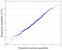
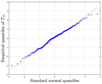
(a)	(b)	(c)

Figure 1: Q-Q (quantile-quantile) plots of $T_{12}$, $T_{13}$ and $T_{14}$ vs. the standard normal distribution in (a), (b) and (c), respectively. The results are reported over 200 independent trials for $r=5$, $p=0.4$ and $\sigma=10^{-3}$.

We begin by checking the validity of Theorem 1. Suppose that one is interested in estimating the inner product $\bm{e}_{i}^{\top}\bm{X}^{\star}\bm{X}^{\star\top}\bm{e}_{j}$ between $\bm{X}^{\star\top}\bm{e}_{i}$ and $\bm{X}^{\star\top}\bm{e}_{j}$ ($i\neq j$). In the Netflix challenge, this might correspond to the similarity between the $i$th user and the $j$th one. As a straightforward consequence of Theorem 1, the normalized estimation error

$$T_{ij}\triangleq\frac{1}{\sqrt{\rho_{ij}}}\left(\bm{e}_{i}^{\top}\bm{X}^{\mathsf{d}}\bm{X}^{\mathsf{d}\top}\bm{e}_{j}-\bm{e}_{i}^{\top}\bm{X}^{\star}\bm{X}^{\star\top}\bm{e}_{j}\right)$$ (3.31)

is extremely close to a standard Gaussian random variable. Here, similar to (3.22), we let

$$\rho_{ij}\triangleq\frac{\sigma^{2}}{p}\left\{\bm{e}_{i}^{\top}\bm{X}^{\mathsf{d}}(\bm{X}^{\mathsf{d}\top}\bm{X}^{\mathsf{d}})^{-1}\bm{X}^{\mathsf{d}\top}\bm{e}_{i}+\bm{e}_{j}^{\top}\bm{X}^{\mathsf{d}}(\bm{X}^{\mathsf{d}\top}\bm{X}^{\mathsf{d}})^{-1}\bm{X}^{\mathsf{d}\top}\bm{e}_{j}\right\}$$ (3.32)

be the empirical estimate of the theoretically predicted variance $\sigma^{2}(\|\bm{U}_{i,\cdot}^{\star}\|_{2}^{2}+\|\bm{U}_{j,\cdot}^{\star}\|_{2}^{2})/p$. As a result, a $95\%$ confidence interval of $\bm{e}_{i}^{\top}\bm{X}^{\star}\bm{X}^{\star\top}\bm{e}_{j}$ would be $[\bm{e}_{i}^{\top}\bm{X}^{\mathsf{d}}\bm{X}^{\mathsf{d}\top}\bm{e}_{j}\pm 1.96\sqrt{\rho_{ij}}]$. For each $(i,j)$, we define $\widehat{\mathsf{Cov}}_{\mathsf{L},(i,j)}$ to be the empirical coverage rate of $\bm{e}_{i}^{\top}\bm{X}^{\star}\bm{X}^{\star\top}\bm{e}_{j}$ over $200$ Monte Carlo simulations. Correspondingly, denote by $\mathsf{Mean}(\widehat{\mathsf{Cov}}_{\mathsf{L}})$ (resp. $\mathsf{Std}(\widehat{\mathsf{Cov}}_{\mathsf{L}})$) the average (resp. the standard deviation) of $\widehat{\mathsf{Cov}}_{\mathsf{L},(i,j)}$ over indices $1\leq i<j\leq n$. Table 2 collects the simulation results for different values of $(r,p,\sigma)$. As can be seen, the reported empirical coverage rates are reasonably close to the nominal level $95\%$. In addition, Figure 1 depicts the Q-Q (quantile-quantile) plots of $T_{12},T_{13}$ and $T_{14}$ vs. the standard Gaussian random variable over 200 Monte Carlo simulations for $r=5$, $p=0.4$ and $\sigma=10^{-3}$. It is clearly seen that all of these are well approximated by a standard Gaussian random variable.

Table 3: Empirical coverage rates of $M_{ij}^{\star}$ for different $(r,p,\sigma)$’s over 200 Monte Carlo trials.

$\vphantom{\sum_{i=1}^{K}}(r,p,\sigma)$	$\mathsf{Mean}(\widehat{\mathsf{Cov}}_{\mathsf{E}})$	$\mathsf{Std}(\widehat{\mathsf{Cov}}_{\mathsf{E}})$
$\vphantom{\frac{1}{2}}(2,0.2,10^{-6})$	0.9380	0.0200
$\vphantom{\frac{1}{2}}(2,0.2,10^{-3})$	0.9392	0.0196
$\vphantom{\frac{1}{2}}(2,0.4,10^{-6})$	0.9455	0.0164
$\vphantom{\frac{1}{2}}(2,0.4,10^{-3})$	0.9456	0.0164
$\vphantom{\frac{1}{2}}(5,0.2,10^{-6})$	0.9226	0.0247
$\vphantom{\frac{1}{2}}(5,0.2,10^{-3})$	0.9271	0.0228
$\vphantom{\frac{1}{2}}(5,0.4,10^{-6})$	0.9410	0.0173
$\vphantom{\frac{1}{2}}(5,0.4,10^{-3})$	0.9417	0.0172

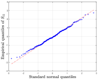
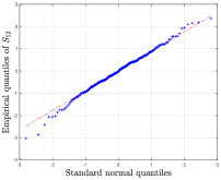
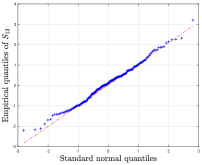
(a)	(b)	(c)

Figure 2: Q-Q (quantile-quantile) plot of $S_{11}$, $S_{12}$ and $S_{13}$ vs. the standard normal distribution in (a), (b) and (c) respectively. The results are reported over 200 independent trials for $r=5$, $p=0.4$ and $\sigma=10^{-3}$.

Next, we turn to Theorem 2, namely the distributional guarantee for the entries of the matrix. Denote

$$S_{ij}\triangleq\frac{1}{\sqrt{v_{ij}}}\left(M_{ij}^{\mathsf{d}}-M_{ij}^{\star}\right),$$ (3.33)

where $v_{ij}$ is the empirical variance defined in (3.22). In view of the $95\%$ confidence interval predicted by Corollary 1, and similar to what have done for the low-rank components, for each $(i,j)$, we define $\widehat{\mathsf{Cov}}_{\mathsf{E},(i,j)}$ to be the empirical coverage rate of $M^{\star}_{ij}$ over $200$ Monte Carlo simulations. Correspondingly, denote by $\mathsf{Mean}(\widehat{\mathsf{Cov}}_{\mathsf{E}})$ (resp. $\mathsf{Std}(\widehat{\mathsf{Cov}}_{\mathsf{E}})$) the average (resp. the standard deviation) of $\widehat{\mathsf{Cov}}_{\mathsf{E},(i,j)}$ over indices $1\leq i,j\leq n$. As before, Table 3 gathers the empirical coverage rates for $M^{\star}_{ij}$ and Figure 2 displays the Q-Q (quantile-quantile) plots of $S_{11},S_{12}$ and $S_{13}$ vs. the standard Gaussian random variable over 200 Monte Carlo trials for $r=5$, $p=0.4$ and $\sigma=10^{-3}$. It is evident that the distribution of $S_{ij}$ matches that of $\mathcal{N}(0,1)$ reasonably well.

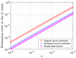
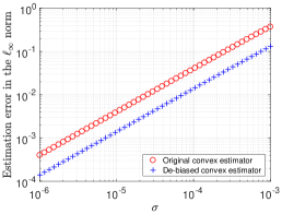
(a)	(b)

Figure 3: (a) Estimation error of $\bm{Z}^{\mathsf{cvx}}$ vs. $\bm{M}^{\mathsf{d}}$ measured in the Frobenius norm. (b) Estimation error of $\bm{Z}^{\mathsf{cvx}}$ vs. $\bm{M}^{\mathsf{d}}$ measured in the $\ell_{\infty}$ norm. The results are averaged over 20 independent trials for $r=5$, $p=0.2$ and $n=1000$.

In addition to the tractable distributional guarantees, the de-biased estimator $\bm{M}^{\mathsf{d}}$ also exhibits superior estimation accuracy compared to the original estimator $\bm{Z}^{\mathsf{cvx}}$ (cf. Theorem 3). Figure 3 reports the estimation error of $\bm{M}^{\mathsf{d}}$ vs. $\bm{Z}^{\mathsf{cvx}}$ measured in both the Frobenius norm and in the $\ell_{\infty}$ norm across difference noise levels. The results are averaged over 20 Monte Carlo simulations for $r=5$, $p=0.2$. It can be seen that the errors of the de-biased estimator are uniformly smaller than that of the original estimator and are much closer to the oracle lower bound. As a result, we recommend using $\bm{M}^{\mathsf{d}}$ even for the purpose of estimation.

We conclude this section with experiments on real data. Similar to [CP10], we use the daily temperature data [NCD19] for 1400 stations across the world in 2018, which results in a $1400\times 365$ data matrix. Inspection on the singular values reveals that the data matrix is nearly low-rank. We vary the observation probability $p$ from $0.5$ to $0.9$ and randomly subsample the data accordingly. Based on the observed temperatures, we then apply the proposed methodology to obtain $95\%$ confidence intervals for all the entries. Table 4 reports the empirical coverage probabilities, the average length of the confidence intervals as well as the estimation error of both $\bm{Z}^{\mathsf{cvx}}$ and $\bm{M}^{\mathsf{d}}$ over 20 independent experiments. It can be seen that the average coverage probabilities are reasonably close to $95\%$ and the confidence intervals are also quite short. In addition, the estimation error of $\bm{M}^{\mathsf{d}}$ is smaller than that of $\bm{Z}^{\mathsf{cvx}}$, which corroborates our theoretical prediction. The discrepancy between the nominal coverage probability and the actual one might arise from the facts that (1) the underlying true temperature matrix is only approximately low-rank, and (2) the noise in the temperature might not be independent.

Table 4: Empirical coverage rates, average lengths of the confidence intervals of the entries as well as the estimation error vs. observation probability $p$. The results are averaged over 20 Monte Carlo trials.

$p$	${\mathsf{Coverage}}$		CI Length		$\|\widehat{\bm{Z}}-\bm{M}^{\star}\|_{\mathrm{F}}/\|\bm{M}^{\star}\|_{\mathrm{F}}$
	Mean	Std	Mean	Std	Convex $\bm{Z}^{\mathsf{cvx}}$	Debiased $\bm{M}^{\mathsf{d}}$
$0.5$	$0.8265$	$0.0016$	$3.6698$	$0.0209$	$0.029$	$0.028$
$0.6$	$0.8268$	$0.0011$	$2.8774$	$0.0098$	$0.025$	$0.023$
$0.7$	$0.8431$	$0.0006$	$2.3426$	$0.0054$	$0.022$	$0.019$
$0.8$	$0.8725$	$0.0003$	$2.0234$	$0.0052$	$0.020$	$0.015$
$0.9$	$0.9093$	$0.0003$	$1.8296$	$0.0072$	$0.018$	$0.011$

3.7 A bit of intuition

We pause to develop some intuition behind the distributional guarantees for the proposed estimators. Bearing in mind the intimate link between convex and nonconvex optimization (cf. (3.5)), it suffices to concentrate on the nonconvex problem (3.4). For the sake of clarity, we further restrict attention to the rank-1 positive semidefinite case where $\bm{M}^{\star}=\bm{x}^{\star}\bm{x}^{\star\top}$ and set $\lambda=0$, where one can focus on

$$\underset{\bm{x}\in\mathbb{R}^{n}}{\textsf{minimize}}\qquad f\left(\bm{x}\right)\triangleq\frac{1}{2}\big{\|}\mathcal{P}_{\Omega}\big{(}\bm{x}\bm{x}^{\top}-\bm{M}\big{)}\big{\|}_{\mathrm{F}}^{2}.$$ (3.34)

Any optimizer $\widehat{\bm{x}}$ of (3.34) would necessarily satisfy the first-order optimality condition

$$\mathcal{P}_{\Omega}\big{(}\widehat{\bm{x}}\widehat{\bm{x}}^{\top}-\bm{M}\big{)}\widehat{\bm{x}}=\bm{0}.$$ (3.35)

We shall also assume that $\widehat{\bm{x}}$ is a reasonably reliable estimate obeying $\widehat{\bm{x}}\approx\bm{x}^{\star}$.

We begin with the no-missing-data case (i.e. $p=1$), which already conveys the key insight. The condition (3.35) simplifies to

$$\widehat{\bm{x}}\widehat{\bm{x}}^{\top}\widehat{\bm{x}}-\bm{x}^{\star}\bm{x}^{\star\top}\widehat{\bm{x}}=\bm{E}\widehat{\bm{x}},$$ (3.36)

which, through a little manipulation, leads to an equivalent decomposition:

$$\|\widehat{\bm{x}}\|_{2}^{2}\left(\widehat{\bm{x}}-\bm{x}^{\star}\right)= \underset{\text{approximately Gaussian}}{\underbrace{\vphantom{\bm{x}^{\star}\left(\bm{x}^{\star}-\widehat{\bm{x}}\right)^{\top}\bm{x}^{\star}}\bm{E}\widehat{\bm{x}}}}+\underset{\text{negligible first-order term}}{\underbrace{\bm{x}^{\star}\left(\bm{x}^{\star}-\widehat{\bm{x}}\right)^{\top}\bm{x}^{\star}}}+\underset{\text{second-order term}}{\underbrace{\bm{x}^{\star}\left(\bm{x}^{\star}-\widehat{\bm{x}}\right)^{\top}\left(\widehat{\bm{x}}-\bm{x}^{\star}\right)}}.$$ (3.37)

Then: (1) the third term of (3.37), which can be viewed as a second-order term (in the sense that it is a quadratic term of $\widehat{\bm{x}}-\bm{x}^{\star}$), becomes vanishingly small when $\widehat{\bm{x}}\approx\bm{x}^{\star}$; (2) while the second term of (3.37) looks like a first-order term, it is natural to conjecture that $\widehat{\bm{x}}-\bm{x}^{\star}$ is sufficiently random and hence $(\widehat{\bm{x}}-\bm{x}^{\star})^{\top}\bm{x}^{\star}\ll\|\widehat{\bm{x}}-\bm{x}^{\star}\|_{2}\|\bm{x}^{\star}\|_{2}$ (i.e. the estimation error is not aligned with $\bm{x}^{\star}$), meaning that this term is also expected to be negligible compared to a typical first-order term (e.g. the term on the left-hand side of 3.37). In summary, these non-rigorous arguments suggest that

$$\|\widehat{\bm{x}}\|_{2}^{2}\left(\widehat{\bm{x}}-\bm{x}^{\star}\right)\,\approx\, \bm{E}\widehat{\bm{x}}.$$ (3.38)

If one can be convinced that $\bm{E}$ and $\widehat{\bm{x}}$ are only weakly dependent, then this means

$$\widehat{\bm{x}}-\bm{x}^{\star}\,\approx\, \frac{1}{\|\widehat{\bm{x}}\|_{2}^{2}}\bm{E}\widehat{\bm{x}}\,\approx\,\frac{1}{\|\bm{x}^{\star}\|_{2}^{2}}\bm{E}\bm{x}^{\star}\,\sim\,\mathcal{N}\Big{(}\bm{0},\frac{\sigma^{2}}{\|\bm{x}^{\star}\|_{2}^{2}}\bm{I}_{n}\Big{)}.$$ (3.39)

Returning to the missing data scenario with $p<1$, everything is based on the following approximation

$$\mathcal{P}_{\Omega}\big{(}\widehat{\bm{x}}\widehat{\bm{x}}^{\top}-\bm{x}^{\star}\bm{x}^{\star\top}\big{)}\widehat{\bm{x}}\approx p\big{(}\widehat{\bm{x}}\widehat{\bm{x}}^{\top}-\bm{x}^{\star}\bm{x}^{\star\top}\big{)}\widehat{\bm{x}};$$

this is certainly expected — using standard concentration arguments — if we “pretend” that $\mathcal{P}_{\Omega}$ and $\widehat{\bm{x}}$ are statistically independent. With this approximation in mind, one can translate (3.35) into

$$p\left(\widehat{\bm{x}}\widehat{\bm{x}}^{\top}\widehat{\bm{x}}-\bm{x}^{\star}\bm{x}^{\star\top}\widehat{\bm{x}}\right)\approx\mathcal{P}_{\Omega}\left(\bm{E}\right)\widehat{\bm{x}}.$$ (3.40)

Repeating the above argument then immediately yields

$$\widehat{\bm{x}}-\bm{x}^{\star}\,\approx\, \frac{1}{\|\widehat{\bm{x}}\|_{2}^{2}}\cdot\frac{1}{p}\mathcal{P}_{\Omega}\left(\bm{E}\right)\widehat{\bm{x}}\,\approx\,\frac{1}{p\|\bm{x}^{\star}\|_{2}^{2}}\cdot\mathcal{P}_{\Omega}\left(\bm{E}\right)\bm{x}^{\star}\overset{\text{approx.}}{\sim}\mathcal{N}\Big{(}\bm{0},\frac{\sigma^{2}}{p\|\bm{x}^{\star}\|_{2}^{2}}\bm{I}_{n}\Big{)}.$$ (3.41)

The case with $\lambda>0$ can be intuitively understood in a very similar way by first de-shrinking the estimate; we omit it here for brevity. We note that these hand-waving arguments can all be made rigorous, which is the main content of the proof.

3.8 Inference based on spectral estimates?

One would naturally be curious about whether there are other estimation procedures that also enable reasonable statistical inference. While this is beyond the scope of the current paper, we take a moment to discuss one alternative: the spectral method, as pioneered by [KMO10a, KMO10b] in the matrix completion problem. In a nutshell, this approach consists in computing a rank-$r$ approximation to $\mathcal{P}_{\Omega}(\bm{M})/p$, which is precisely the spectral initialization widely used in a two-stage nonconvex algorithm (cf. Algorithm 1) [KMO10b, SL16, CW15, CCF18, MWCC17]. While inference has not been, as far as we know, the focus of prior work on spectral methods, the recent papers [AFWZ17, MWCC17] hinted at the possibility of characterizing the distribution of the spectral estimate. Take a simple symmetric rank-1 case for example (i.e. $\bm{M}^{\star}=\bm{x}^{\star}\bm{x}^{\star\top}$ with $\|\bm{x}^{\star}\|_{2}=1$): the leading eigenvector $\bm{u}^{\mathsf{spectral}}$ of $\mathcal{P}_{\Omega}(\bm{M})/p$ often admits the following approximation (up to a global sign)

$$\bm{u}^{\mathsf{spectral}} \approx\frac{1}{p}\mathcal{P}_{\Omega}(\bm{M})\bm{x}^{\star}.$$

Expanding $\mathcal{P}_{\Omega}(\bm{M})=p\bm{x}^{\star}\bm{x}^{\star\top}+\mathcal{P}_{\Omega}(\bm{x}^{\star}\bm{x}^{\star\top})-p\bm{x}^{\star}\bm{x}^{\star\top}+\mathcal{P}_{\Omega}(\bm{E})$, we arrive at

$$\bm{u}^{\mathsf{spectral}} \approx\bm{x}^{\star}\bm{x}^{\star\top}\bm{x}^{\star}+\Big{(}\frac{1}{p}\mathcal{P}_{\Omega}(\bm{x}^{\star}\bm{x}^{\star\top})-\bm{x}^{\star}\bm{x}^{\star\top}\Big{)}\bm{x}^{\star}+\frac{1}{p}\mathcal{P}_{\Omega}(\bm{E})\bm{x}^{\star},$$

which is equivalent to

$$\bm{u}^{\mathsf{spectral}} -\bm{x}^{\star}\approx\underset{\text{noise effect}}{\underbrace{\vphantom{\Big{(}\frac{1}{p}\mathcal{P}_{\Omega}(\bm{x}^{\star}\bm{x}^{\star\top})-\bm{x}^{\star}\bm{x}^{\star\top}\Big{)}\bm{x}^{\star}}\frac{1}{p}\mathcal{P}_{\Omega}(\bm{E})\bm{x}^{\star}}}+\underset{\text{effect of random sub-sampling}}{\underbrace{\Big{(}\frac{1}{p}\mathcal{P}_{\Omega}(\bm{x}^{\star}\bm{x}^{\star\top})-\bm{x}^{\star}\bm{x}^{\star\top}\Big{)}\bm{x}^{\star}}}.$$ (3.42)

In words, two major factors dictate the uncertainty of the spectral estimate: (1) the additive Gaussian noise (cf. the 1st term on the right-hand side of (3.42)), and (2) random sub-sampling (in particular, the randomness incurred by employing the sub-sampled $\mathcal{P}_{\Omega}(\bm{x}^{\star}\bm{x}^{\star\top})/p$ to approximate the truth $\bm{x}^{\star}\bm{x}^{\star\top}$). Given that the random sub-sampling effect cannot be ignored at all, the spectral estimates often suffer from a much larger estimation error (and hence a higher degree of uncertainty) compared to either the convex or the nonconvex estimates. In truth, this random sub-sampling effect does not go away even when the noise vanishes. Consequently, uncertainty quantification based on the spectral estimates may not be the most desirable option.

4 Prior art

Matrix completion.

Low-rank matrix completion, or more broadly, low-rank matrix recovery, is a fundamental task that permeates through a wide spectrum of applications in science, engineering, and finance (e.g. [RS05, SY07, CC14, FSZZ18, CCG15, ZPL15, BN06, CC18b, FWZ19, KS11, CZ16, KX15, FLM13, DR17, CDDD19, DPVW14, SZ12, FS11]). A paper of this length is unable to review all papers motivating and contributing to this enormous subject; interested readers are referred to [DR16, CC18a] for extensive discussions of motivating applications as well as the exciting recent development.

Numerous algorithms have been proposed to solve this problem efficiently, with two paradigms being arguably the most widely used: convex relaxation and nonconvex optimization. We briefly review the literature contributing to these two paradigms.

• Convex relaxation was largely popularized by the seminal works [Faz02, RFP10, CR09]. In the absence of noise, it has been shown that nuclear norm minimization, which can be solved by semidefinite programming, achieves minimal sample complexity under mild conditions [Gro11, Rec11, Che15]. When the observed entries are further corrupted by noise, Candès and Plan [CP10] provided the first theoretical guarantee regarding the estimation accuracy of perhaps the most natural convex relaxation algorithm. While the theory might be tight for certain adversarial scenarios (as shown by the recent work [KS19]), it is loose by some large factor under the natural random noise model. This statistical guarantee has been partially improved later on by two papers [NW12, KLT11] under proper modifications to the convex program (e.g. enforcing an additional spikiness constraint [NW12, Klo14], or modifying the squared loss [KLT11]). Nevertheless, the error bounds provided in these papers (and their follow-ups) remain suboptimal, unless the typical size of the noise is sufficiently large. Our recent work [CCF⁺19] establishes near-optimal statistical guarantees — when the estimation errors are measured by the Frobenius norm, the spectral norm, and the $\ell_{2,\infty}$ norm — for a wide range of noise levels when $r=O(1)$. All of these estimation guarantees, however, come with a hidden and likely large pre-constant, which do not serve the inferential purpose well.

• Nonconvex optimization algorithms, as pioneered by [KMO10a, Sre04], become increasingly more popular for solving various low-rank factorization problems, due to their appealing computational complexities [JNS13, CLS15, CC17, TBS⁺16, SL16, ZL16, CCFM19, WZG16, CLL19]. For instance, the gradient-based nonconvex methods have been analyzed for noisy matrix completion [KMO10b, CW15, MWCC17, CCF⁺19], which are shown to achieve near-optimal statistical accuracy and linear-time convergence guarantees all at once. Going beyond gradient methods, we note that other nonconvex methods (e.g. [RS05, JMD10, WYZ12, JNS13, FRW11, Van13, LXY13, Har14, JKN16, RT11, WCCL16, DC18, ZWL15, ZWYG18, MSL19, CCD⁺19]) and landscape properties [GLM16, CL17, GJZ17, ZSL19, ZJSL18, SXZ19] have been largely explored as well. The interested readers are referred to [CLC19] for an in-depth discussion. One limitation, however, is that the theoretical guarantees provided for nonconvex algorithms often exhibit sub-optimal dependency in the rank $r$ of the unknown matrix; for instance, most theory requires a sample complexity of at least $nr^{2}$ (in fact, often much larger than $nr^{2}$). This is outperformed by the convex relaxation approach.

Despite these recent developments, very little work has investigated statistical inference for noisy matrix completion. While [CKLN18, CKL16, CN15, CEGN15] discussed the construction of “honest” confidence regions, the volume of these regions is dependent on some (possibly huge) hidden constants, thus resulting in over-coverage. Perhaps the closest to our paper is the recent work [Xia18], which investigated inference for low-rank trace regression. Employing a closely related de-biased estimator with sample splitting, the paper [Xia18] established asymptotic normality of a certain projected distance between the estimate and the truth. The result therein, however, requires a sampling mechanism obeying the restricted isometry property (e.g. i.i.d. Gaussian designs), which fails to hold for matrix completion. Also, our approach does not require sample splitting — a technique that is convenient for analysis but conservative in constructing confidence regions. Another work by Cai et al. [CLR16] developed a unified approach to provide inference guarantees for linear inverse problems including low-rank matrix estimation. Their results, however, require the sample size to exceed the total dimension $n^{2}$ even under the Gaussian design. Finally, a recent line of work [MX17] explored uncertainty quantification under the Bayesian setting, hypothesizing on a special prior regarding the true matrix. This departs drastically from the scenario considered herein.

Inference in high-dimensional problems.

Inference in high-dimensional sparse regression has received much attention in the last few years [WR09, ZZ14, BCH11, vdGBRD14, JM14b, DBMM15, CG17, NL17, NNLL18, LSST16, LTTT14, MMB09, DBZ17, ZC17, BFL⁺18]. Our inferential approach is partly inspired by the recent developments on this topic, particularly with regard to the de-biased / de-sparsified estimators proposed for Lasso. More specifically, recognizing the non-negligible bias of the Lasso estimate

$$\widehat{\bm{\beta}}\triangleq\arg\min_{\bm{\beta}}\,\,\frac{1}{2}\|\bm{y}-\bm{X}\bm{\beta}\|_{2}^{2}+\lambda\|\bm{\beta}\|_{1},$$ (4.1)

A line of work [ZZ14, vdGBRD14, JM14a] came up with a linear transformation of $\widehat{\bm{\beta}}$ of the form

$$\bm{\beta}^{\mathrm{d}}\triangleq\widehat{\bm{\beta}}+\bm{L}\bm{X}^{\top}\big{(}\bm{y}-\bm{X}\widehat{\bm{\beta}}\big{)},$$ (4.2)

where $\bm{L}$ is some matrix to be designed, and $\bm{X}^{\top}\big{(}\bm{y}-\bm{X}\widehat{\bm{\beta}}\big{)}$ corresponds to the negative gradient of the squared loss at $\widehat{\bm{\beta}}$, or equivalently, the (scaled) sub-gradient of the $\ell_{1}$ norm at $\widehat{\bm{\beta}}$. If $\bm{L}$ is properly chosen, then $\bm{\beta}^{\mathrm{d}}$ is able to correct the bias of this nonlinear estimator $\bm{\beta}$, while controlling the degree of uncertainty. Many follow-up papers have investigated the design of $\bm{L}$ as well as the resulting inferential guarantees [ZZ14, vdGBRD14, JM14a, JM15].

Interestingly, our de-biased estimator (3.7) for matrix completion admits a very similar form as (4.2). To see this, recall that our de-biased estimator is given by

$$\bm{M}^{\mathsf{d}}=\mathcal{P}_{\text{rank-}r}\big{(}\bm{Z}-\tfrac{1}{p}\mathcal{P}_{\Omega}\big{(}\bm{Z}\big{)}+\tfrac{1}{p}\mathcal{P}_{\Omega}\big{(}\bm{M}\big{)}\big{)},$$

where $\bm{Z}$ can be either $\bm{Z}^{\mathsf{cvx}}$ or $\bm{X}^{\mathsf{ncvx}}\bm{Y}^{\mathsf{ncvx}\top}$ (see Table 1). Let $T$ be the tangent space of the set of rank-$r$ matrices at $\bm{Z}^{\mathsf{cvx},r}$ (resp. $\bm{X}^{\mathsf{ncvx}}\bm{Y}^{\mathsf{ncvx}\top}$) in the convex (resp. nonconvex) case, and $\mathcal{P}_{T}$ be the projection operator onto $T$. Somewhat surprisingly, replacing $\mathcal{P}_{\text{rank-}r}$ by $\mathcal{P}_{T}$ does not affect the de-biased estimator by much, in the sense that

$$\bm{M}^{\mathsf{d}}\approx\mathcal{P}_{T}\big{(}\bm{Z}-\tfrac{1}{p}\mathcal{P}_{\Omega}\big{(}\bm{Z}\big{)}+\tfrac{1}{p}\mathcal{P}_{\Omega}\big{(}\bm{M}\big{)}\big{)}.$$ (4.3)

In addition, recognizing that $\bm{Z}$ almost lies within the tangent space $T$,one can rewrite

$$\bm{M}^{\mathsf{d}}\approx\bm{Z}-\tfrac{1}{p}\mathcal{P}_{T}\mathcal{P}_{\Omega}\big{(}\bm{Z}-\bm{M}\big{)},$$ (4.4)

a fact to be made precise in Section 5.1. This bears a striking resemblance to the de-biasing approach developed for Lasso — the term $\mathcal{P}_{\Omega}\big{(}\bm{Z}-\bm{M}^{\star}\big{)}$ represents the gradient of the squared loss $0.5\|\mathcal{P}_{\Omega}\big{(}\bm{Z}-\bm{M}\big{)}\|_{\mathrm{F}}^{2}$ (or equivalently, the negative sub-gradient of the nuclear norm) at $\bm{Z}$, and $\mathcal{P}_{T}$ is the linear operator we pick. To the best of our knowledge, no de-biasing approach — with rigorous theoretical guarantees and without sample splitting — has been proposed and analyzed for matrix completion in prior literature. In addition, we note that our de-biased estimator for matrix completion achieves full statistical efficiency in terms of both the rates and the pre-constant; in comparison, the commonly used de-biased estimators for sparse linear regression typically fall short of achieving the best possible estimation accuracy, unless additional thresholding procedures are enforced.

Finally, de-biased estimators have been put forward to tackle other high-dimensional problems, including but not limited to generalized linear models [vdGBRD14, NL17], graphical models [JVDG15, RSZZ15, MLL17, JvdG17], sparse PCA [JvdG18], treatment effects estimation [CCD⁺18, AIW18]. These are beyond the scope of the current paper.

5 Architecture of the proof

This section outlines the main steps for establishing Theorem 1 and Theorem 2. Before starting, we introduce some useful notation. For convenience of presentation, we insert the factor $1/p$ into (3.4) and redefine the nonconvex loss function as

$$f\left(\bm{X},\bm{Y}\right)\triangleq\frac{1}{2p}\left\|\mathcal{P}_{\Omega}\left(\bm{X}\bm{Y}^{\top}-\bm{M}\right)\right\|_{\mathrm{F}}^{2}+\frac{\lambda}{2p}\left\|\bm{X}\right\|_{\mathrm{F}}^{2}+\frac{\lambda}{2p}\left\|\bm{Y}\right\|_{\mathrm{F}}^{2}.$$ (5.1)

In addition, for each $1\leq j,k\leq n$, we define the indicator $\delta_{jk}\triangleq\operatorname{\mathds{1}}\{(j,k)\in\Omega\}$, which is a Bernoulli random variable with mean $p$.

We also note that Theorem 1 (resp. Theorem 2) is subsumed by Theorem 5 (resp. Theorem 6). As a result, we shall focus on establishing Theorem 5 (resp. Theorem 6) when it comes to estimating low-rank factors (resp. the entries of the matrix).

Theorem 5.

Suppose that the sample complexity meets $n^{2}p\geq C\kappa^{4}\mu^{2}r^{2}n\log^{3}n$ for some sufficiently large constant $C>0$ and the noise obeys $\sigma\sqrt{(\kappa^{4}\mu rn\log n)/p}\leq c\sigma_{\min}$ for some sufficiently small constant $c>0$. Then the decomposition in Theorem 1 remains valid, except that the residual matrices $\bm{\Psi}_{\bm{X}},\bm{\Psi}_{\bm{Y}}\in\mathbb{R}^{n\times r}$ satisfy, with probability at least $1-O(n^{-3})$, that

$$\max\big{\{}\left\|\bm{\Psi}_{\bm{X}}\right\|_{2,\infty},\left\|\bm{\Psi}_{\bm{Y}}\right\|_{2,\infty}\big{\}}\lesssim\frac{\sigma}{\sqrt{p\sigma_{\min}}}\left(\,\frac{\sigma}{\sigma_{\min}}\sqrt{\frac{\kappa^{7}\mu rn\log n}{p}}+\sqrt{\frac{\kappa^{7}\mu^{3}r^{3}\log^{2}n}{np}}\,\right).$$ (5.2)

Theorem 6.

Instate the assumptions of Theorem 5. Recall the definition of $v_{ij}^{\star}$ in (3.17). Then one has the following decomposition

$$M_{ij}^{\mathsf{{d}}}-M_{ij}^{\star}=g_{ij}+\Delta_{ij},$$ (5.3)

where $g_{ij}\sim\mathcal{N}(0,v_{ij}^{\star})$ and the residual obeys — with probability exceeding $1-O(n^{-10})$ — that

$$\left|\Delta_{ij}\right|\lesssim\left(\left\|\bm{U}_{i,\cdot}^{\star}\right\|_{2}+\left\|\bm{V}_{j,\cdot}^{\star}\right\|_{2}\right)\frac{\sigma}{\sqrt{p}}\left(\frac{\sigma}{\sigma_{\min}}\sqrt{\frac{\kappa^{8}\mu rn\log n}{p}}+\sqrt{\frac{\kappa^{8}\mu^{3}r^{3}\log^{2}n}{np}}\right)+\left(\frac{\sigma}{\sqrt{\sigma_{\min}}}\sqrt{\frac{\kappa^{3}\mu r\log n}{p}}\right)^{2}.$$

5.1 Near equivalence between convex and nonconvex estimators

Note that Theorem 5 and Theorem 6 are concerned with the de-biased estimators built upon both convex and nonconvex estimates. At first glance, one needs to establish theoretical guarantees for each of them separately. Fortunately, as alluded to previously (cf. (3.5)), the convex and nonconvex estimates are extremely close — a fact that has been established in [CCF⁺19]. The proximity of these two estimates naturally extends to the de-biased estimators constructed based on them. As a result, it suffices to concentrate on proving the theorems for any of these estimators; the claims for the other one follow immediately.

The following key lemma formalizes this argument, which will be established in Appendix C (see also Figure 4 for numerical evidence). Before continuing, we remind the readers of the key notation (see Appendix B for precise definitions):

• $(\bm{X}^{\mathsf{ncvx}},\bm{Y}^{\mathsf{ncvx}})$: an approximate solution to the nonconvex problem (3.4) (see Appendix A.1);

• $\bm{M}^{\mathsf{cvx,d}},\bm{X}^{\mathsf{cvx,d}},\bm{Y}^{\mathsf{cvx,d}}$: the de-biased estimators built upon the convex optimizer $\bm{Z}^{\mathsf{cvx}}$;

• $\bm{M}^{\mathsf{ncvx,d}},\bm{X}^{\mathsf{ncvx,d}},\bm{Y}^{\mathsf{ncvx,d}}$: the de-biased estimators built upon the nonconvex estimate $(\bm{X}^{\mathsf{ncvx}},\bm{Y}^{\mathsf{ncvx}})$.

Our proximity result is this:

Lemma 3.

Suppose that the sample size obeys $n^{2}p\geq C\kappa^{4}\mu^{2}r^{2}n\log^{3}n$ for some sufficiently large constant $C>0$ and the noise satisfies $\sigma\sqrt{(\kappa^{4}\mu nr\log n)/p}\leq c\sigma_{\min}$ for some sufficiently small constant $c>0$. Set $\lambda=C_{\lambda}\sigma\sqrt{np}$ with some large enough constant $C_{\lambda}>0$.

1. With probability at least $1-O(n^{-10})$, one has

   $$\max\left\{\left\|\bm{M}^{\mathsf{cvx,d}}-\bm{X}^{\mathsf{ncvx,d}}\bm{Y}^{\mathsf{ncvx,d}\top}\right\|_{\mathrm{F}},\left\|\bm{M}^{\mathsf{ncvx,d}}-\bm{X}^{\mathsf{ncvx,d}}\bm{Y}^{\mathsf{ncvx,d}\top}\right\|_{\mathrm{F}}\right\} \lesssim\frac{1}{n^{4}}\cdot\sigma\sqrt{\frac{n}{p}},$$ (5.4a)

   $$\min_{\bm{R}\in\mathcal{O}^{r\times r}}\sqrt{\left\|\bm{X}^{\mathsf{cvx,d}}\bm{R}-\bm{X}^{\mathsf{ncvx,d}}\right\|_{\mathrm{F}}^{2}+\left\|\bm{Y}^{\mathsf{cvx,d}}\bm{R}-\bm{Y}^{\mathsf{ncvx,d}}\right\|_{\mathrm{F}}^{2}} \lesssim\frac{1}{n^{3}}\cdot\frac{\sigma}{\sqrt{\sigma_{\min}}}\sqrt{\frac{n}{p}},$$ (5.4b)

   where $\mathcal{O}^{r\times r}$ is the set of $r\times r$ rotation matrices.

2. With probability exceeding $1-O(n^{-10})$, one has

   $$\left\|\bm{M}^{\mathsf{ncvx,d}}-\left[\bm{X}^{\mathsf{ncvx}}\bm{Y}^{\mathsf{ncvx}\top}-p^{-1}\mathcal{P}_{T}\mathcal{P}_{\Omega}\left(\bm{X}^{\mathsf{ncvx}}\bm{Y}^{\mathsf{ncvx}\top}-\bm{M}\right)\right]\right\|_{\mathrm{F}}\lesssim\frac{1}{n^{4}}\cdot\sigma\sqrt{\frac{n}{p}},$$ (5.5)

   where $T$ is the tangent space of the set of rank-$r$ matrices at $\bm{X}^{\mathsf{ncvx}}\bm{Y}^{\mathsf{ncvx}\top}$. The same holds true if we replace $\bm{X}^{\mathsf{ncvx}}\bm{Y}^{\mathsf{ncvx}\top}$ with $\bm{Z}^{\mathsf{cvx}}$ and replace $T$ with the tangent space at $\bm{Z}^{\mathsf{cvx},r}=\mathcal{P}_{\mathrm{rank}\text{-}r}(\bm{Z}^{\mathsf{cvx}})$ .

In short, the first part of Lemma 3 tells us that

$$\bm{M}^{\mathsf{cvx,d}} \approx\bm{X}^{\mathsf{ncvx,d}}\bm{Y}^{\mathsf{ncvx,d}\top}\approx\bm{M}^{\mathsf{ncvx,d}},$$ (5.6a)

$$\big{(}\bm{X}^{\mathsf{cvx,d}},\bm{Y}^{\mathsf{cvx,d}}\big{)} \approx\big{(}\bm{X}^{\mathsf{ncvx,d}},\bm{Y}^{\mathsf{ncvx,d}}\big{)}\qquad\qquad(\text{up to global rotation}),$$ (5.6b)

whereas the second part of Lemma 3 justifies that the proposed de-biased estimator is closely approximated by a linearized version (cf. (4.4)). Note that this linearized form bears a resemblance to the de-biased estimators developed for sparse linear regression [ZZ14, vdGBRD14, JM14a].

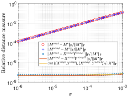
Figure 4: The relative estimation errors of $\bm{M}^{\mathsf{cvx,d}}$ and $\bm{M}^{\mathsf{ncvx,d}}$ and related quantities in Lemma 3 vs. the standard deviation $\sigma$ of the noise. Here, $\mathsf{dist}((\bm{X}^{\mathsf{cvx,d}},\bm{Y}^{\mathsf{cvx,d}}),(\bm{X}^{\mathsf{ncvx,d}},\bm{Y}^{\mathsf{ncvx,d}}))$ is defined to be the left-hand side of (5.4b). The results, which are averaged over 20 trials, are reported for $n=1000$, $r=5$, $p=0.2$, and $\lambda=5\sigma\sqrt{np}$. As can be seen, the difference between $\bm{M}^{\mathsf{cvx,d}}$, $\bm{M}^{\mathsf{ncvx,d}}$ and $\bm{X}^{\mathsf{ncvx,d}}\bm{Y}^{\mathsf{ncvx,d}\top}$, as well as the distance $\mathsf{dist}((\bm{X}^{\mathsf{cvx,d}},\bm{Y}^{\mathsf{cvx,d}}),(\bm{X}^{\mathsf{ncvx,d}},\bm{Y}^{\mathsf{ncvx,d}}))$, are all significantly smaller than the estimation errors.

With Lemma 3 in place, we shall, from now on, focus on proving the main theorems for the nonconvex estimators, viz.

1. establishing Theorem 5 for the de-shrunken low-rank factors $(\bm{X}^{\mathsf{ncvx,d}},\bm{Y}^{\mathsf{ncvx,d}})$;

2. establishing Theorem 6 for the de-biased matrix estimator $\bm{X}^{\mathsf{ncvx,d}}\bm{Y}^{\mathsf{ncvx,d}\top}$.

To simplify the presentation hereafter, we shall use the following notation throughout the rest of this section:

• $(\bm{X},\bm{Y})$: the nonconvex estimate $(\bm{X}^{\mathsf{ncvx}},\bm{Y}^{\mathsf{ncvx}})$;

• $(\bm{X}^{\mathsf{d}},\bm{Y}^{\mathsf{d}})$: the de-shrunken estimate defined in (3.8) based on $(\bm{X},\bm{Y})=(\bm{X}^{\mathsf{ncvx}},\bm{Y}^{\mathsf{ncvx}})$;

• $\bm{M}^{\mathsf{d}}\triangleq\bm{X}^{\mathsf{d}}\bm{Y}^{\mathsf{d}\top}$.

5.2 A precise characterization of the de-shrunken low-rank factors

We start with a precise characterization of the de-shrunken low-rank factors $\bm{X}^{\mathsf{d}}$ and $\bm{Y}^{\mathsf{d}}$, which paves the way for demonstrating both Theorem 5 and Theorem 6.

Lemma 4 (Decompositions of low-rank factors).

Denote

$$\bm{A}\triangleq\frac{1}{p}\mathcal{P}_{\Omega}\left(\bm{X}\bm{Y}^{\top}-\bm{X}^{\star}\bm{Y}^{\star\top}\right)-\left(\bm{X}\bm{Y}^{\top}-\bm{X}^{\star}\bm{Y}^{\star\top}\right).$$ (5.7)

One has the following decompositions for $\bm{X}^{\mathsf{d}}$ and $\bm{Y}^{\mathsf{d}}$

$$\bm{X}^{\mathsf{d}} =\frac{1}{p}\mathcal{P}_{\Omega}\left(\bm{E}\right)\bm{Y}^{\mathsf{d}}\left(\bm{Y}^{\mathsf{d}\top}\bm{Y}^{\mathsf{d}}\right)^{-1}+\bm{X}^{\star}\bm{Y}^{\star\top}\bm{Y}^{\mathsf{d}}\left(\bm{Y}^{\mathsf{d}\top}\bm{Y}^{\mathsf{d}}\right)^{-1}-\bm{A}\bm{Y}^{\mathsf{d}}\left(\bm{Y}^{\mathsf{d}\top}\bm{Y}^{\mathsf{d}}\right)^{-1}$$

$$\quad+\nabla_{\bm{X}}f\left(\bm{X},\bm{Y}\right)\Big{(}\bm{I}_{r}+\frac{\lambda}{p}\left(\bm{Y}^{\top}\bm{Y}\right)^{-1}\Big{)}^{1/2}\left(\bm{Y}^{\mathsf{d}\top}\bm{Y}^{\mathsf{d}}\right)^{-1}+\bm{X}\bm{\Delta}_{\mathsf{balancing}};$$ (5.8a)

$$\bm{Y}^{\mathsf{d}} =\frac{1}{p}\left[\mathcal{P}_{\Omega}\left(\bm{E}\right)\right]^{\top}\bm{X}^{\mathsf{d}}\left(\bm{X}^{\mathsf{d}\top}\bm{X}^{\mathsf{d}}\right)^{-1}+\bm{Y}^{\star}\bm{X}^{\star\top}\bm{X}^{\mathsf{d}}\left(\bm{X}^{\mathsf{d}\top}\bm{X}^{\mathsf{d}}\right)^{-1}-\bm{A}^{\top}\bm{X}^{\mathsf{d}}\left(\bm{X}^{\mathsf{d}\top}\bm{X}^{\mathsf{d}}\right)^{-1}$$

$$\quad+\nabla_{\bm{Y}}f\left(\bm{X},\bm{Y}\right)\Big{(}\bm{I}_{r}+\frac{\lambda}{p}\left(\bm{X}^{\top}\bm{X}\right)^{-1}\Big{)}^{1/2}\left(\bm{X}^{\mathsf{d}\top}\bm{X}^{\mathsf{d}}\right)^{-1}-\bm{Y}\bm{\Delta}_{\mathsf{balancing}}.$$ (5.8b)

Here, we denote

$$\bm{\Delta}_{\mathsf{balancing}}\triangleq\Big{(}\bm{I}_{r}+\frac{\lambda}{p}\left(\bm{X}^{\top}\bm{X}\right)^{-1}\Big{)}^{1/2}-\Big{(}\bm{I}_{r}+\frac{\lambda}{p}\left(\bm{Y}^{\top}\bm{Y}\right)^{-1}\Big{)}^{1/2},$$ (5.9)

which measures the imbalance between the low-rank factors $\bm{X}$ and $\bm{Y}$.

Proof.

The claims follow from straightforward algebraic manipulations; see Appendix D.1. ∎

We make a few observations regarding Lemma 4. Take the decomposition of $\bm{X}^{\mathsf{d}}$ (5.8a) as an example:

• First, the term $\bm{A}\bm{Y}^{\mathsf{d}}(\bm{Y}^{\mathsf{d}\top}\bm{Y}^{\mathsf{d}})^{-1}$ vanishes when we have full observations, i.e. $p=1$. Second, the terms involving $\nabla_{\bm{X}}f(\bm{X},\bm{Y})$ and $\bm{\Delta}_{\mathsf{balancing}}$ are both zero if $(\bm{X},\bm{Y})$ is an exact stationary point of $f(\cdot,\cdot)$; to see this, it is not hard to verify that any stationary point of $f(\cdot,\cdot)$ necessarily satisfies $\bm{X}^{\top}\bm{X}=\bm{Y}^{\top}\bm{Y}$, which in turn implies $\bm{\Delta}_{\mathsf{balancing}}=\bm{0}$. Consequently, the last three terms in (5.8a) are expected to be small when $p$ is sufficiently large and $(\bm{X},\bm{Y})$ is near a stationary point.

• Turning to the first two terms in (5.8a), we note that the second term of (5.8a) is close to $\bm{X}^{\star}$ (up to rotation) if $\bm{Y}^{\mathrm{d}}$ is a nearly accurate approximation to $\bm{Y}^{\star}$. In comparison, the first term $\mathcal{P}_{\Omega}(\bm{E})\bm{Y}^{\mathsf{d}}(\bm{Y}^{\mathsf{d}\top}\bm{Y}^{\mathsf{d}})^{-1}/p$ has to do with a collection of Gaussian random variables, which accounts for the main uncertainty term.

We shall make precise these arguments in subsequent subsections.

5.3 Taking global rotation into account

In order to invoke the decompositions of $\bm{X}^{\mathsf{d}}$ and $\bm{Y}^{\mathsf{d}}$ (cf. Lemma 4) to characterize the estimation errors, we still need to incorporate the (unrecoverable) rotation matrix. From now on, we shall focus primarily on the factor $\bm{X}^{\mathsf{d}}$. The claims on the other factor $\bm{Y}^{\mathsf{d}}$ can be easily obtained via symmetry.

Denote

$$\overline{\bm{X}}^{\mathsf{d}}\triangleq\bm{X}^{\mathsf{d}}\bm{H}^{\mathsf{d}}\qquad\text{and}\qquad\overline{\bm{Y}}^{\mathsf{d}}\triangleq\bm{Y}^{\mathsf{d}}\bm{H}^{\mathsf{d}},$$ (5.10)

where we recall that $\bm{H}^{\mathsf{d}}$ is the rotation matrix that best aligns $(\bm{X}^{\mathsf{d}},\bm{Y}^{\mathsf{d}})$ and $(\bm{X}^{\star},\bm{Y}^{\star})$ (see (3.12)). Substituting the identity

$$\bm{Y}^{\mathsf{d}}\left(\bm{Y}^{\mathsf{d}\top}\bm{Y}^{\mathsf{d}}\right)^{-1}\bm{H}^{\mathsf{d}}=\bm{Y}^{\mathsf{d}}\bm{H}^{\mathsf{d}}\left(\bm{H}^{\mathsf{d}\top}\bm{Y}^{\mathsf{d}\top}\bm{Y}^{\mathsf{d}}\bm{H}^{\mathsf{d}}\right)^{-1}=\overline{\bm{Y}}^{\mathsf{d}}\big{(}\overline{\bm{Y}}^{\mathsf{d}\top}\overline{\bm{Y}}^{\mathsf{d}}\big{)}^{-1}$$

into the decomposition (5.8a), we arrive at

$$\bm{X}^{\mathsf{d}}\bm{H}^{\mathsf{d}}-\bm{X}^{\star} =\frac{1}{p}\mathcal{P}_{\Omega}\left(\bm{E}\right)\overline{\bm{Y}}^{\mathsf{d}}\big{(}\overline{\bm{Y}}^{\mathsf{d}\top}\overline{\bm{Y}}^{\mathsf{d}}\big{)}^{-1}+\bm{X}^{\star}\left[\bm{Y}^{\star\top}\overline{\bm{Y}}^{\mathsf{d}}\big{(}\overline{\bm{Y}}^{\mathsf{d}\top}\overline{\bm{Y}}^{\mathsf{d}}\big{)}^{-1}-\bm{I}_{r}\right]-\bm{A}\overline{\bm{Y}}^{\mathsf{d}}\big{(}\overline{\bm{Y}}^{\mathsf{d}\top}\overline{\bm{Y}}^{\mathsf{d}}\big{)}^{-1}$$

$$\quad+\nabla_{\bm{X}}f\left(\bm{X},\bm{Y}\right)\Big{(}\bm{I}_{r}+\frac{\lambda}{p}\left(\bm{Y}^{\top}\bm{Y}\right)^{-1}\Big{)}^{1/2}\left(\bm{Y}^{\mathsf{d}\top}\bm{Y}^{\mathsf{d}}\right)^{-1}\bm{H}^{\mathsf{d}}+\bm{X}\bm{\Delta}_{\mathsf{balancing}}\bm{H}^{\mathsf{d}}$$

$$=\frac{1}{p}\mathcal{P}_{\Omega}\left(\bm{E}\right)\bm{Y}^{\star}\left(\bm{Y}^{\star\top}\bm{Y}^{\star}\right)^{-1}+\bm{\Phi}_{\bm{X}}.$$ (5.11)

Here, the term $\bm{\Phi}_{\bm{X}}\in\mathbb{R}^{n\times r}$ is defined to be

$$\bm{\Phi}_{\bm{X}} \triangleq\underbrace{\frac{1}{p}\mathcal{P}_{\Omega}\left(\bm{E}\right)\left[\overline{\bm{Y}}^{\mathsf{d}}\big{(}\overline{\bm{Y}}^{\mathsf{d}\top}\overline{\bm{Y}}^{\mathsf{d}}\big{)}^{-1}-\bm{Y}^{\star}\left(\bm{Y}^{\star\top}\bm{Y}^{\star}\right)^{-1}\right]}_{:=\bm{\Phi}_{1}}+\underbrace{\vphantom{\frac{1}{p}\mathcal{P}_{\Omega}\left(\bm{E}\right)\left[\overline{\bm{Y}}^{\mathsf{d}}\big{(}\overline{\bm{Y}}^{\mathsf{d}\top}\overline{\bm{Y}}^{\mathsf{d}}\big{)}^{-1}-\bm{Y}^{\star}\left(\bm{Y}^{\star\top}\bm{Y}^{\star}\right)^{-1}\right]}\bm{X}^{\star}\left[\bm{Y}^{\star\top}\overline{\bm{Y}}^{\mathsf{d}}\big{(}\overline{\bm{Y}}^{\mathsf{d}\top}\overline{\bm{Y}}^{\mathsf{d}}\big{)}^{-1}-\bm{I}_{r}\right]}_{:=\bm{\Phi}_{2}}$$

$$\quad\underbrace{-\vphantom{\Big{(}\bm{I}_{r}+\frac{\lambda}{p}\left(\bm{Y}^{\top}\bm{Y}\right)^{-1}\Big{)}^{1/2}}\bm{A}\overline{\bm{Y}}^{\mathsf{d}}\big{(}\overline{\bm{Y}}^{\mathsf{d}\top}\overline{\bm{Y}}^{\mathsf{d}}\big{)}^{-1}}_{:=\bm{\Phi}_{3}}+\underbrace{\nabla_{\bm{X}}f\left(\bm{X},\bm{Y}\right)\Big{(}\bm{I}_{r}+\frac{\lambda}{p}\left(\bm{Y}^{\top}\bm{Y}\right)^{-1}\Big{)}^{1/2}\left(\bm{Y}^{\mathsf{d}\top}\bm{Y}^{\mathsf{d}}\right)^{-1}\bm{H}^{\mathsf{d}}+\bm{X}\bm{\Delta}_{\mathsf{balancing}}\bm{H}^{\mathsf{d}}}_{:=\bm{{\Phi}}_{4}},$$ (5.12)

where $\bm{A}$ is defined in (5.7). To establish Theorem 5, it remains to (1) demonstrate that $\bm{\Phi}_{\bm{X}}$ has small $\ell_{2,\infty}$ norm, and (2) show that $\mathcal{P}_{\Omega}(\bm{E})\bm{Y}^{\star}(\bm{Y}^{\star\top}\bm{Y}^{\star})^{-1}/p$ is approximately a Gaussian random matrix. These two steps constitute the main content of the next subsection.

5.4 Key lemmas for establishing Theorem 5

We now state five key lemmas. Taking these collectively and substituting them into (5.11) immediately establish Theorem 5.

We shall start by controlling the term $\bm{\Phi}_{1}$ as defined in (5.12).

Lemma 5 (Negligibility of $\bm{\Phi}_{1}$).

Suppose that the sample complexity obeys $n^{2}p\geq C\kappa^{4}\mu^{2}r^{2}n\log^{3}n$ for some sufficiently large constant $C>0$ and the noise satisfies $\sigma\sqrt{(\kappa^{4}\mu rn\log n)/p}\leq c\sigma_{\min}$ for some sufficiently small constant $c<0$. Then with probability at least $1-O(n^{-10})$, we have

$$\left\|\bm{{\Phi}}_{1}\right\|_{2,\infty}\lesssim\frac{\sigma}{\sqrt{p\sigma_{\min}}}\cdot\frac{{\sigma}}{\sigma_{\min}}\sqrt{{\frac{{\kappa^{3}\mu rn\log n}}{p}}}.$$

Proof.

Fix any $1\leq j\leq n$. If the de-shrunken estimate $\overline{\bm{Y}}^{\mathsf{d}}$ were independent of the randomness in the $j$th row of the matrix, i.e. $\bm{e}_{j}^{\top}\mathcal{P}_{\Omega}(\bm{E})$, then $\|\bm{e}_{j}^{\top}\bm{\Phi}_{1}\|_{2}$ would be well controlled. This hypothesis is certainly false, as $\overline{\bm{Y}}^{\mathsf{d}}$ clearly depends on $\bm{e}_{j}^{\top}\mathcal{P}_{\Omega}(\bm{E})$. Nevertheless, by exploiting the leave-one-out technique recently used in [EKBB⁺13, EK15, AFWZ17, MWCC17, CFMW19, CCF⁺19, CLL19, DC18], one can properly decouple the dependency and establish the desired bound. See Appendix D.2.∎

The next lemma controls the size of $\|\bm{\Phi}_{2}\|_{2,\infty}$. In essence, the term $\bm{\Phi}_{2}$ measures the difference between the estimate $\overline{\bm{Y}}^{\mathsf{d}}$ and the true signal $\bm{Y}^{\star}$; the closer these two are, the smaller $\|\bm{\Phi}_{2}\|_{2,\infty}$ should be. See Appendix D.3 for the proof of the following result.

Lemma 6 (Negligibility of $\bm{\Phi}_{2}$).

Suppose that the sample complexity obeys $n^{2}p\geq C\kappa^{4}\mu^{2}r^{2}n\log^{3}n$ for some sufficiently large constant $C>0$ and the noise satisfies $\sigma\sqrt{(\kappa^{4}\mu rn\log n)/p}\leq c\sigma_{\min}$ for some sufficiently small constant $c<0$. Then with probability exceeding $1-O(n^{-10})$, one has

$$\left\|\bm{\Phi}_{2}\right\|_{2,\infty}\lesssim\frac{\sigma}{\sqrt{p\sigma_{\min}}}\left(\kappa\frac{\sigma}{\sigma_{\min}}\sqrt{\frac{\kappa^{7}\mu rn}{p}}+\sqrt{\frac{\kappa^{7}\mu^{3}r^{3}\log n}{np}}\right).$$

Moving on to $\bm{\Phi}_{3}$ and $\bm{\Phi}_{4}$, one has the following lemmas.

Lemma 7 (Negligibility of $\bm{\Phi}_{3}$).

Suppose that the sample complexity obeys $n^{2}p\geq C\kappa^{4}\mu^{2}r^{2}n\log^{3}n$ for some sufficiently large constant $C>0$ and the noise satisfies $\sigma\sqrt{(\kappa^{4}\mu rn\log n)/p}\leq c\sigma_{\min}$ for some sufficiently small constant $c<0$. Then with probability exceeding $1-O(n^{-10})$, we have

$$\left\|\bm{{\Phi}}_{3}\right\|_{2,\infty}\lesssim\frac{\sigma}{\sqrt{p\sigma_{\min}}}\sqrt{\frac{\kappa^{5}\mu^{3}r^{3}\log^{2}n}{np}}.$$

Proof.

It is straightforward to check that when $p=1$, one has $\|\bm{\Phi}_{3}\|_{2,\infty}=\|\bm{A}\|=0$, where we recall the definition of $\bm{A}$ in (5.7). Therefore, one expects $\|\bm{\Phi}_{3}\|_{2,\infty}$ to be small when $p$ is sufficiently large. See Appendix D.4.∎

Lemma 8 (Negligibility of $\bm{\Phi}_{4}$).

Suppose that the sample complexity obeys $n^{2}p\geq C\kappa^{4}\mu^{2}r^{2}n\log^{3}n$ for some sufficiently large constant $C>0$ and the noise satisfies $\sigma\sqrt{(\kappa^{4}\mu rn\log n)/p}\leq c\sigma_{\min}$ for some sufficiently small constant $c<0$. Then with probability at least $1-O(n^{-10})$, one has

$$\left\|\bm{{\Phi}}_{4}\right\|_{2,\infty}\lesssim\frac{\sigma}{\sqrt{p\sigma_{\min}}}\cdot\frac{1}{n^{4}}.$$

Proof.

It is easily seen that the size of $\bm{\Phi}_{4}$ depends on how close $(\bm{X},\bm{Y})$ is to a stationary point of $f(\cdot,\cdot)$. For instance, in the extreme case where $(\bm{X},\bm{Y})$ is an exact stationary point, then one would have $\bm{\Phi}_{4}=\bm{0}$. See Appendix D.5.∎

The last lemma asserts that $\mathcal{P}_{\Omega}(\bm{E})\bm{Y}^{\star}(\bm{Y}^{\star\top}\bm{Y}^{\star})^{-1}/p$ is, in some sense, close to a zero-mean Gaussian random matrix with the desired covariance.

Lemma 9 (Approximate Gaussianity of $\mathcal{P}_{\Omega}(\bm{E})\bm{Y}^{\star}(\bm{Y}^{\star\top}\bm{Y}^{\star})^{-1}/p$).

Suppose that the sample size obeys $n^{2}p\geq C\kappa^{2}\mu rn\log^{3}n$ for some sufficiently large constant $C>0$. Then one has the decomposition

$$\frac{1}{p}\mathcal{P}_{\Omega}\left(\bm{E}\right)\bm{Y}^{\star}\left(\bm{Y}^{\star\top}\bm{Y}^{\star}\right)^{-1}=\bm{Z}_{\bm{X}}+\bm{\Delta}_{\bm{X}},$$

where each row of $\bm{Z}_{\bm{X}}\in\mathbb{R}^{n\times r}$ is independent and identically distributed according to

$$\bm{Z}_{\bm{X}}^{\top}\bm{e}_{j}\overset{\mathrm{i.i.d}}{\sim}\mathcal{N}\Big{(}\bm{0},\frac{\sigma^{2}}{p}\left(\bm{\Sigma}^{\star}\right)^{-1}\Big{)},\qquad\mathrm{for}\quad 1\leq j\leq n.$$

In addition, with probability at least $1-O(n^{-10})$, the remaining term $\bm{\Delta}_{\bm{X}}\in\mathbb{R}^{n\times r}$ obeys

$$\left\|\bm{\Delta}_{\bm{X}}\right\|_{2,\infty}\lesssim\frac{\sigma}{\sqrt{p\sigma_{\min}}}\sqrt{\frac{\kappa^{2}\mu r^{2}\log^{2}n}{np}}.$$

Proof.

Fix any $1\leq j\leq n$. The $j$th row, namely $\bm{e}_{j}^{\top}[\mathcal{P}_{\Omega}(\bm{E})\bm{Y}^{\star}(\bm{Y}^{\star\top}\bm{Y}^{\star})^{-1}/p]$ is conditionally Gaussian in the sense that

$$\bm{e}_{j}^{\top}\left[\frac{1}{p}\mathcal{P}_{\Omega}\left(\bm{E}\right)\bm{Y}^{\star}\left(\bm{Y}^{\star\top}\bm{Y}^{\star}\right)^{-1}\right]\,\Big{|}\,\Omega\ \sim\ \mathcal{N}\Big{(}\bm{0},\frac{\sigma^{2}}{p}\Big{(}\,\frac{1}{p}\sum_{k=1}^{n}\delta_{jk}\left(\bm{\Sigma}^{\star}\right)^{-1}\left(\bm{Y}_{k,\cdot}^{\star}\right)^{\top}\bm{Y}_{k,\cdot}^{\star}\left(\bm{\Sigma}^{\star}\right)^{-1}\Big{)}\Big{)},$$

where we recall that $\delta_{jk}=\operatorname{\mathds{1}}\{(j,k)\in\Omega\}$. Recognize that the conditional covariance matrix concentrates sharply around its expectation, i.e. $\sigma^{2}(\bm{\Sigma}^{\star})^{-1}/p$, which is the covariance matrix of $\bm{Z}_{\bm{X}}^{\top}\bm{e}_{j}$ that we are after. Hence, one can expect that $\mathcal{P}_{\Omega}(\bm{E})\bm{Y}^{\star}(\bm{Y}^{\star\top}\bm{Y}^{\star})^{-1}/p$ is, marginally, not too far from a Gaussian random matrix. This argument can be carried out formally; see Appendix D.6. ∎

5.5 From low-rank factors to matrix entries (Proof of Theorem 6)

We now turn attention to inference on the matrix entries, by establishing Theorem 6. Towards this, we first make the following observation: for any $1\leq i,j\leq n$,

$$M_{ij}^{\mathsf{{d}}}-M_{ij}^{\star} =\bm{{e}}_{i}^{\top}\text{$\overline{{\bm{{X}}}}$}^{\mathsf{{d}}}\overline{{\bm{{Y}}}}^{\mathsf{{d}}\top}\bm{{e}}_{j}-\bm{{e}}_{i}^{\top}\bm{{X}}^{\star}\bm{{Y}}^{\star\top}\bm{{e}}_{j}$$

$$=\bm{e}_{i}^{\top}\big{(}\overline{\bm{X}}^{\mathsf{d}}-\bm{X}^{\star}\big{)}\bm{Y}^{\star\top}\bm{e}_{j}+\bm{e}_{i}^{\top}\bm{X}^{\star}\big{(}\overline{\bm{Y}}^{\mathsf{d}}-\bm{Y}^{\star}\big{)}^{\top}\bm{e}_{j}+\bm{e}_{i}^{\top}\big{(}\overline{\bm{X}}^{\mathsf{d}}-\bm{X}^{\star}\big{)}\big{(}\overline{\bm{Y}}^{\mathsf{d}}-\bm{Y}^{\star}\big{)}^{\top}\bm{e}_{j}.$$ (5.13)

One can readily apply the decompositions in Theorem 5 to obtain

$$\bm{e}_{i}^{\top}\big{(}\overline{\bm{X}}^{\mathsf{d}}-\bm{X}^{\star}\big{)}\bm{Y}^{\star\top}\bm{e}_{j} =\bm{e}_{i}^{\top}\bm{Z}_{\bm{X}}\bm{Y}^{\star\top}\bm{e}_{j}+\bm{e}_{i}^{\top}\bm{\Psi}_{\bm{X}}\bm{Y}^{\star\top}\bm{e}_{j},$$ (5.14)

$$\bm{e}_{i}^{\top}\bm{X}^{\star}\big{(}\overline{\bm{Y}}^{\mathsf{d}}-\bm{Y}^{\star}\big{)}^{\top}\bm{e}_{j} =\bm{e}_{i}^{\top}\bm{X}^{\star}\bm{Z}_{\bm{Y}}^{\top}\bm{e}_{j}+\bm{e}_{i}^{\top}\bm{X}^{\star}\bm{\Psi}_{\bm{Y}}^{\top}\bm{e}_{j}.$$ (5.15)

Take the preceding three identities collectively to reach

$$M_{ij}^{\mathsf{{d}}}-M_{ij}^{\star} =\underbrace{\bm{e}_{i}^{\top}\bm{Z}_{\bm{X}}\bm{Y}^{\star\top}\bm{e}_{j}+\bm{e}_{i}^{\top}\bm{X}^{\star}\bm{Z}_{\bm{Y}}^{\top}\bm{e}_{j}}_{:=\Theta_{ij}}$$

$$\quad+\underbrace{\bm{e}_{i}^{\top}\bm{\Psi}_{\bm{X}}\bm{Y}^{\star\top}\bm{e}_{j}+\bm{e}_{i}^{\top}\bm{X}^{\star}\bm{\Psi}_{\bm{Y}}^{\top}\bm{e}_{j}+\bm{e}_{i}^{\top}\big{(}\overline{\bm{X}}^{\mathsf{d}}-\bm{X}^{\star}\big{)}\big{(}\overline{\bm{Y}}^{\mathsf{d}}-\bm{Y}^{\star}\big{)}^{\top}\bm{e}_{j}}_{:=\Lambda_{ij}}.$$

Following the same route as in Section 5.4, one can verify that $\Theta_{ij}=\bm{e}_{i}^{\top}\bm{Z}_{\bm{X}}\bm{Y}^{\star\top}\bm{e}_{j}+\bm{e}_{i}^{\top}\bm{X}^{\star}\bm{Z}_{\bm{Y}}^{\top}\bm{e}_{j}$ is approximately Gaussian, whereas the residual term $\Lambda_{ij}$ is small in magnitude. These claims are formally stated in the next two lemmas, with the proofs deferred to Appendix E.

Lemma 10 ($\mathsf{Negligibility\;of}$ $\Lambda_{ij}$).

Suppose that the sample complexity obeys $n^{2}p\geq C\kappa^{4}\mu^{2}r^{2}n\log^{3}n$ for some sufficiently large constant $C>0$ and the noise satisfies $\sigma\sqrt{(\kappa^{4}\mu rn\log n)/p}\leq c\sigma_{\min}$ for some sufficiently small constant $c<0$. Then with probability exceeding $1-O(n^{-10})$, one has

$$\left|\Lambda_{ij}\right|\lesssim\left(\left\|\bm{U}_{i,\cdot}^{\star}\right\|_{2}+\left\|\bm{V}_{j,\cdot}^{\star}\right\|_{2}\right)\frac{\sigma}{\sqrt{p}}\left(\frac{\sigma}{\sigma_{\min}}\sqrt{\frac{\kappa^{8}\mu rn\log n}{p}}+\sqrt{\frac{\kappa^{8}\mu^{3}r^{3}\log^{2}n}{np}}\right)+\left(\frac{\sigma}{\sqrt{\sigma_{\min}}}\sqrt{\frac{\kappa^{3}\mu r\log n}{p}}\right)^{2}.$$

Lemma 11 ($\mathsf{Approximate\;Gaussianity\;of}$ $\Theta_{ij}$).

Suppose that $np\geq C\kappa^{2}\mu r^{2}\log^{2}n$ for some sufficiently large constant $C>0$. Then we have the decomposition

$$\Theta_{ij}=\bm{e}_{i}^{\top}\bm{Z}_{\bm{X}}\bm{Y}^{\star\top}\bm{e}_{j}+\bm{e}_{i}^{\top}\bm{X}^{\star}\bm{Z}_{\bm{Y}}^{\top}\bm{e}_{j}=g_{ij}+\theta_{ij},$$

where $g_{ij}\sim\mathcal{N}(0,v_{ij}^{\star})$ and the remaining term $\theta_{ij}$ satisfies — with probability exceeding $1-O(n^{-10})$ — that

$$\left|\theta_{ij}\right|\lesssim\frac{\sigma}{\sqrt{p}}\sqrt{\frac{\kappa^{2}\mu r\log n}{np}}\min\left\{\left\|\bm{U}_{i,\cdot}^{\star}\right\|_{2},\left\|\bm{V}_{j,\cdot}^{\star}\right\|_{2}\right\}.$$

Putting the above two lemmas together immediately establishes Theorem 6 and hence Theorem 2.

6 Discussion

The present paper makes progress towards inference and uncertainty quantification for noisy matrix completion, by developing simple de-biased estimators that admit tractable and accurate distributional characterizations. While we have achieved some early success in accomplishing this, our results are likely sub-optimal in the following aspects:

• Dependency on the rank and the condition number. To enable valid inference, our sample complexity (cf. (3.13) and (3.18a)) scales sub-optimally with the rank $r$ and the condition number $\kappa$. The sub-optimality can be understood through comparisons with the sample size requirement $O(nr\log^{2}n)$ in the noise-free settings, which is independent of $\kappa$ and matches the information limit (up to some $\log$ factor). Improving such dependency calls for more refined analysis techniques.

• Detection of the size of the entries. On one hand, when the size of the entry $M_{ij}^{\star}$ is moderately large (cf. (3.18b)), Corollary 1 allows us to construct a valid confidence interval for it. On the other hand, when $\|\bm{U}_{i,\cdot}^{\star}\|_{2}+\|\bm{V}_{j,\cdot}^{\star}\|_{2}$ vanishes, Theorem 5 tells us that the estimation error $M_{ij}^{\mathsf{d}}-M_{ij}^{\star}$ is better approximated by the inner product of two independent Gaussian random vectors. It remains to be seen how to determine whether $\|\bm{U}_{i,\cdot}^{\star}\|_{2}+\|\bm{V}_{j,\cdot}^{\star}\|_{2}$ is too small.

• Low signal-to-noise (SNR) regime. Our theory operates under the moderate-to-high SNR regime, where $\sigma^{2}_{\min}/\sigma^{2}$ (which is proportional to the SNR) is required to exceed the order of $n/p$; see the conditions in Theorem 5. It is unclear whether the connection between the convex and the nonconvex estimators hold in the low SNR regime. How to conduct inference in such a scenario is an important future direction.

In addition, our investigation has been dedicated to a natural random model, which by no means covers the most general settings of practical interest. There are numerous possible extensions that merit future investigation:

• Approximate low-rank structure. Our current theory is built upon the exact low-rank structure of $\bm{{M}}^{\star}$. Realistically, the matrix of interest is often only approximately low-rank. It is of great interest to study how to carry out statistical inference under such imperfect structural assumptions.

• More general sampling patterns. This paper operates under the uniform random sampling assumption, which might sometimes be off in practical situations. It would be interesting to investigate whether our results in this paper can extend to more general non-uniform sampling patterns (e.g. [NW12]).

• Extensions to robust PCA, sparse PCA, and 1-bit matrix completion. A variety of important extensions of matrix completion have been explored in prior literature, including but not limited to the case with sparse outliers (i.e. robust PCA [CLMW11, CSPW11]), the case where the matrix of interest is simultaneously sparse and low-rank (i.e. sparse PCA [ZHT06, CMW13]), and the case where only finite-bit observations are available (i.e. 1-bit matrix completion [DPVW14, CZ13]). Performing valid uncertainty assessment for these scenarios requires non-trivial extensions of the link between convex and nonconvex optimization.

• Other loss functions. In the estimation stage, one might sometimes prefer other loss functions beyond the penalized squared loss. This might arise from either statistical considerations (e.g. employing a penalized Poisson log-likelihood to accommodate Poisson noise [CX16]), or computational concerns (e.g. adopting a non-smooth loss to improve convergence [CCD⁺19]). It would be of fundamental importance to develop a unified inferential framework that covers a broader family of loss functions.

Appendix A Preliminaries

In this section, we gather several notation and preliminary facts that are useful throughout the analysis. All the proofs, if needed, are deferred to Appendix I.

A.1 Algorithmic details of nonconvex optimization

To begin with, we make precise the algorithm used to minimize the nonconvex loss function (5.1). Specifically, we describe the following details that are crucial for us to implement Algorithm 1:

• Set the initial point to be $(\bm{X}^{0},\bm{Y}^{0})=(\bm{X}^{\star},\bm{Y}^{\star})$ or the spectral initialization as in [MWCC17, CLL19];

• Set the stepsize $\eta\asymp 1/(n^{6}\kappa^{3}\sigma_{\max})$;

• Set the maximum number of iterations to be $t_{0}\asymp n^{23}$;

• The returned estimate is $(\bm{X}^{\mathsf{ncvx}},\bm{Y}^{\mathsf{ncvx}})\triangleq(\bm{X}^{t_{\star}},\bm{Y}^{t_{\star}})$, where

  $$t_{\star}\,\triangleq\,\min\,\left\{0\leq t\leq t_{0}\,\Big{|}\,\left\|\nabla f\left(\bm{X}^{t},\bm{Y}^{t}\right)\right\|_{\mathrm{F}}\leq\frac{1}{n^{5}}\frac{\lambda}{p}\sqrt{\sigma_{\min}}\right\}.$$ (A.1)

  In words, we run gradient descent in Algorithm 1 until we reach a point whose gradient is exceedingly small.

Remark 6 (Spectral initialization).

Many of the preliminary facts below were established for the case $(\bm{X}^{0},\bm{Y}^{0})=(\bm{X}^{\star},\bm{Y}^{\star})$ [CCF⁺19], which is certainly not implementable in practice, however, it serves as a good proxy for studying the convex estimator. Fortunately, the same theoretical guarantees stated in Appendix A.2 can be readily established for spectral initialization using almost the same arguments adopted in [MWCC17, CLL19, CCF⁺19]. We omit this part mainly for the sake of brevity.

To facilitate analysis, we introduce a set of auxiliary nonconvex loss functions. For any $1\leq j\leq n$, define

$$f^{(j)}\left(\bm{X},\bm{Y}\right)\triangleq\frac{1}{2p}\left\|\mathcal{P}_{\Omega_{-j},\cdot}\left(\bm{X}\bm{Y}^{\top}-\bm{M}\right)\right\|_{\mathrm{F}}^{2}+\frac{1}{2}\left\|\mathcal{P}_{j,\cdot}\left(\bm{X}\bm{Y}^{\top}-\bm{M}\right)\right\|_{\mathrm{F}}^{2}+\frac{\lambda}{2p}\left\|\bm{X}\right\|_{\mathrm{F}}^{2}+\frac{\lambda}{2p}\left\|\bm{Y}\right\|_{\mathrm{F}}^{2},$$ (A.2)

where $\mathcal{P}_{\Omega_{-j,\cdot}}:\mathbb{R}^{n\times n}\mapsto\mathbb{R}^{n\times n}$ (resp. $\mathcal{P}_{j,\cdot}(\cdot)$) denotes the orthogonal projection onto the subspace of matrices that vanish outside of $\{(i,k)\in\Omega\,|\,i\neq j\}$ (resp. $\{(i,k)\,|\,i=j\}$). Let

$$(\bm{X}^{(j)},\bm{Y}^{(j)})=(\bm{X}^{t_{\star},(j)},\bm{Y}^{t_{\star},(j)})$$ (A.3)

be the nonconvex estimate returned by this auxiliary algorithm (i.e. Algorithm 2), which serves as an approximate solution to (A.2).

Algorithm 2 Gradient descent for solving the auxiliary nonconvex problem (A.2).

  Suitable initialization: $(\bm{X}^{0,(j)},\bm{Y}^{0,(j)})=(\bm{X}^{\star},\bm{Y}^{\star})$

  Gradient updates: for $t=0,1,\ldots,t_{\star}-1$ do

  

$$\bm{X}^{t+1,(j)}= \bm{X}^{t,(j)}-\eta\nabla_{\bm{X}}f^{(j)}\big{(}\bm{X}^{t,(j)},\bm{Y}^{t,(j)}\big{)};$$ (A.4a)

$$\bm{Y}^{t+1,(j)}= \bm{Y}^{t,(j)}-\eta\nabla_{\bm{Y}}f^{(j)}\big{(}\bm{X}^{t,(j)},\bm{Y}^{t,(j)}\big{)}.$$ (A.4b)

A.2 Properties of approximate nonconvex solutions

This subsection gathers the properties of the (approximate) nonconvex solutions. Throughout this subsection, we use the shorthand

$$(\bm{X},\bm{Y})=(\bm{X}^{\mathsf{ncvx}},\bm{Y}^{\mathsf{ncvx}})$$ (A.5)

and recall the definition of $(\bm{X}^{(j)},\bm{Y}^{(j)})$ in (A.3). The regularization parameter is chosen to satisfy

$$\lambda\asymp\sigma\sqrt{np}.$$ (A.6)

To further simplify the presentation, we introduce $\bm{F}^{\star}$, $\bm{F}$, $\bm{F}^{\mathrm{d}}$, $\bm{F}^{\mathrm{d},(j)}\in\mathbb{R}^{2n\times r}$ as follows

$$\bm{F}^{\star}\triangleq\left[\begin{array}[]{c}\bm{X}^{\star}\\ \bm{Y}^{\star}\end{array}\right];\quad\bm{F}\triangleq\left[\begin{array}[]{c}\bm{X}\\ \bm{Y}\end{array}\right];\quad\bm{F}^{\mathsf{d}}\triangleq\left[\begin{array}[]{c}\bm{X}^{\mathsf{d}}\\ \bm{Y}^{\mathsf{d}}\end{array}\right];\quad\bm{F}^{\mathsf{d},(j)}\triangleq\left[\begin{array}[]{c}\bm{X}^{\mathsf{d},(j)}\\ \bm{Y}^{\mathsf{d},(j)}\end{array}\right],$$ (A.7)

and define

$$\bm{H} \triangleq\arg\min_{\bm{R}\in\mathcal{O}^{r\times r}}\left\|\bm{F}\bm{R}-\bm{F}^{\star}\right\|_{\mathrm{F}}^{2}=\arg\min_{\bm{R}\in\mathcal{O}^{r\times r}}\left\{\left\|\bm{X}\bm{R}-\bm{X}^{\star}\right\|_{\mathrm{F}}^{2}+\left\|\bm{Y}\bm{R}-\bm{Y}^{\star}\right\|_{\mathrm{F}}^{2}\right\},$$ (A.8a)

$$\bm{H}^{(j)} \triangleq\arg\min_{\bm{R}\in\mathcal{O}^{r\times r}}\bigl{\|}\bm{F}^{(j)}\bm{R}-\bm{F}^{\star}\bigr{\|}_{\mathrm{F}}^{2}=\arg\min_{\bm{R}\in\mathcal{O}^{r\times r}}\left\{\bigl{\|}\bm{X}^{(j)}\bm{R}-\bm{X}^{\star}\bigr{\|}_{\mathrm{F}}^{2}+\bigl{\|}\bm{Y}^{(j)}\bm{R}-\bm{Y}^{\star}\bigr{\|}_{\mathrm{F}}^{2}\right\},$$ (A.8b)

$$\bm{R}^{(j)} \triangleq\arg\min_{\bm{R}\in\mathcal{O}^{r\times r}}\bigl{\|}\bm{F}^{(j)}\bm{R}-\bm{F}\bm{H}\bigr{\|}_{\mathrm{F}}^{2}=\arg\min_{\bm{R}\in\mathcal{O}^{r\times r}}\left\{\bigl{\|}\bm{X}^{(j)}\bm{R}-\bm{X}\bm{H}\bigr{\|}_{\mathrm{F}}^{2}+\bigl{\|}\bm{Y}^{(j)}\bm{R}-\bm{Y}\bm{H}\bigr{\|}_{\mathrm{F}}^{2}\right\},$$ (A.8c)

$$\bm{H}^{\mathsf{d},(j)} \triangleq\arg\min_{\bm{R}\in\mathcal{O}^{r\times r}}\bigl{\|}\bm{F}^{\mathsf{d},(j)}\bm{R}-\bm{F}^{\star}\bigr{\|}_{\mathrm{F}}^{2}=\arg\min_{\bm{R}\in\mathcal{O}^{r\times r}}\left\{\bigl{\|}\bm{X}^{\mathsf{d},(j)}\bm{R}-\bm{X}^{\star}\bigr{\|}_{\mathrm{F}}^{2}+\bigl{\|}\bm{Y}^{\mathsf{d},(j)}\bm{R}-\bm{Y}^{\star}\bigr{\|}_{\mathrm{F}}^{2}\right\}.$$ (A.8d)

The claims stated below hold under the sample complexity and the noise condition presumed in [CCF⁺19, Theorem 1] (see also Theorem 5 in the current manuscript)

$$n^{2}p\gg\kappa^{4}\mu^{2}r^{2}n\log^{3}n\quad\text{and}\quad\sigma\sqrt{\frac{n}{p}}\ll\frac{\sigma_{\min}}{\sqrt{\kappa^{4}\mu r\log n}}.$$

1. The first set of facts is related to $(\bm{X},\bm{Y})$. In view of [CCF⁺19], $\bm{F}$ is a faithful estimate of $\bm{F}^{\star}$, in the sense that

   $$\left\|\bm{F}\bm{H}-\bm{F}^{\star}\right\|_{\mathrm{F}} \lesssim\frac{\sigma}{\sigma_{\min}}\sqrt{\frac{n}{p}}\left\|\bm{X}^{\star}\right\|_{\mathrm{F}},$$ (A.9a)

   $$\left\|\bm{F}\bm{H}-\bm{F}^{\star}\right\| \lesssim\frac{\sigma}{\sigma_{\min}}\sqrt{\frac{n}{p}}\left\|\bm{X}^{\star}\right\|,$$ (A.9b)

   $$\left\|\bm{F}\bm{H}-\bm{F}^{\star}\right\|_{\mathrm{2,\infty}} \lesssim\kappa\frac{\sigma}{\sigma_{\min}}\sqrt{\frac{n\log n}{p}}\left\|\bm{F}^{\star}\right\|_{2,\infty}$$ (A.9c)

   hold with probability exceeding $1-O(n^{-10})$. In addition, on the same high-probability event, one has

   $$\left\|\nabla f\left(\bm{X},\bm{Y}\right)\right\|_{\mathrm{F}} \leq\frac{1}{n^{5}}\frac{\lambda}{p}\sqrt{\sigma_{\min}};$$ (A.10)

   $$\left\|\bm{X}^{\top}\bm{X}-\bm{Y}^{\top}\bm{Y}\right\|_{\mathrm{F}} \leq\frac{1}{n^{5}}\frac{\sigma}{\sigma_{\min}}\sqrt{\frac{n}{p}}\sigma_{\max}\leq\frac{1}{n^{5}}\sigma_{\max};$$ (A.11)

   $$\max\left\{\left\|\bm{Z}^{\mathsf{cvx}}-\bm{X}\bm{Y}^{\top}\right\|_{\mathrm{F}},\left\|\bm{Z}^{\mathsf{cvx},r}-\bm{X}\bm{Y}^{\top}\right\|_{\mathrm{F}}\right\} \lesssim\frac{\kappa^{2}}{n^{5}}\frac{\lambda}{p}.$$ (A.12)

   In words, the first claim ensures that $(\bm{X},\bm{Y})$ is an approximate stationary point of $f(\cdot,\cdot)$; the second bound tells us that $(\bm{X},\bm{Y})$ is nearly balanced, in the sense that $\bm{X}^{\top}\bm{X}\approx\bm{Y}^{\top}\bm{Y}$; the last one formalizes the proximity between the convex solution and the nonconvex one; see also (3.5).

2. We move on to the properties of the de-shrunken estimator $(\bm{X}^{\mathsf{d}},\bm{Y}^{\mathrm{d}})$, which is defined in (3.8). Specifically, we can show that (see Appendix I)

   $$\left\|\bm{F}^{\mathsf{d}}\bm{H}-\bm{F}^{\star}\right\| \lesssim\frac{\sigma}{\sigma_{\min}}\sqrt{\frac{n}{p}}\left\|\bm{X}^{\star}\right\|,$$ (A.13a)

   $$\left\|\bm{F}^{\mathsf{d}}\bm{H}^{\mathsf{d}}-\bm{F}^{\star}\right\| \lesssim\kappa\frac{\sigma}{\sigma_{\min}}\sqrt{\frac{n}{p}}\left\|\bm{X}^{\star}\right\|,$$ (A.13b)

   $$\left\|\bm{F}^{\mathsf{d}}\bm{H}^{\mathsf{d}}-\bm{F}^{\star}\right\|_{\mathrm{F}} \lesssim\frac{\sigma}{\sigma_{\min}}\sqrt{\frac{n}{p}}\left\|\bm{X}^{\star}\right\|_{\mathrm{F}},$$ (A.13c)

   $$\left\|\bm{F}^{\mathsf{d}}\bm{H}^{\mathsf{d}}-\bm{F}^{\star}\right\|_{2,\infty} \lesssim\kappa\frac{\sigma}{\sigma_{\min}}\sqrt{\frac{n\log n}{p}}\left\|\bm{F}^{\star}\right\|_{2,\infty},$$ (A.13d)

   $$\left\|\bm{X}^{\mathsf{d}\top}\bm{X}^{\mathsf{d}}-\bm{Y}^{\mathsf{d}\top}\bm{Y}^{\mathsf{d}}\right\| \lesssim\frac{\kappa}{n^{5}}\frac{\sigma}{\sigma_{\min}}\sqrt{\frac{n}{p}}\sigma_{\max}$$ (A.13e)

   hold with probability at least $1-O(n^{-10})$.

3. As has been shown in [CCF⁺19], the leave-one-out auxiliary point $(\bm{X}^{(j)},\bm{Y}^{(j)})$ satisfies

   $$\bigl{\|}\bm{F}^{(j)}\bm{R}^{(j)}-\bm{F}\bm{H}\bigr{\|}_{\mathrm{F}} \lesssim\frac{\sigma}{\sigma_{\min}}\sqrt{\frac{n\log n}{p}}\left\|\bm{F}^{\star}\right\|_{2,\infty},$$ (A.14a)

   $$\bigl{\|}\bm{F}^{(j)}\bm{H}^{(j)}-\bm{F}\bm{H}\bigr{\|}_{\mathrm{F}} \lesssim\kappa\frac{\sigma}{\sigma_{\min}}\sqrt{\frac{n\log n}{p}}\left\|\bm{F}^{\star}\right\|_{2,\infty},$$ (A.14b)

   $$\bigl{\|}\bm{F}^{(j)}\bm{H}^{(j)}-\bm{F}^{\star}\bigr{\|} \lesssim\frac{\sigma}{\sigma_{\min}}\sqrt{\frac{n}{p}}\left\|\bm{X}^{\star}\right\|,$$ (A.14c)

   $$\bigl{\|}\bm{{F}}^{(j)}\bm{{R}}^{(j)}-\bm{{F}}^{\star}\bigr{\|}_{2,\infty} \lesssim\kappa\frac{\sigma}{\sigma_{\min}}\sqrt{\frac{n\log n}{p}}\left\|\bm{{F}}^{\star}\right\|_{2,\infty}$$ (A.14d)

   with probability exceeding $1-O(n^{-10})$.

4. Parallel to the transition from $(\bm{X},\bm{Y})$ to $(\bm{X}^{\mathsf{d}},\bm{Y}^{\mathsf{d}})$, we set

   $$\bm{X}^{\mathrm{d},(j)}\triangleq\bm{X}^{(j)}\Big{(}\bm{I}_{r}+\frac{\lambda}{p}\big{(}\bm{X}^{(j)\top}\bm{X}^{(j)}\big{)}^{-1}\Big{)}^{1/2}\quad\text{and}\quad\bm{Y}^{\mathrm{d},(j)}\triangleq\bm{Y}^{(j)}\Big{(}\bm{I}_{r}+\frac{\lambda}{p}\big{(}\bm{Y}^{(j)\top}\bm{Y}^{(j)}\big{)}^{-1}\Big{)}^{1/2}$$ (A.15)

   to be the de-shrunken estimators of $\bm{X}^{(j)}$ and $\bm{Y}^{(j)}$, respectively. We shall demonstrate in Appendix I that, with probability at least $1-O(n^{-10})$,

   $$\bigl{\|}\bm{F}^{\mathsf{d},(j)}\bm{H}^{\mathsf{d},(j)}-\bm{F}^{\star}\bigr{\|} \lesssim\kappa\frac{\sigma}{\sigma_{\min}}\sqrt{\frac{n}{p}}\left\|\bm{X}^{\star}\right\|,$$ (A.16a)

   $$\bigl{\|}\bm{F}^{\mathsf{d},(j)}\bm{H}^{\mathsf{d},(j)}-\bm{F}^{\star}\bigr{\|}_{2,\infty} \lesssim\kappa\frac{\sigma}{\sigma_{\min}}\sqrt{\frac{n\log n}{p}}\left\|\bm{F}^{\star}\right\|_{2,\infty},$$ (A.16b)

   $$\bigl{\|}\bm{F}^{\mathsf{d},(j)}\bm{H}^{\mathsf{d},(j)}-\bm{F}^{\mathsf{d}}\bm{H}^{\mathsf{d}}\bigr{\|} \lesssim\kappa\frac{\sigma}{\sigma_{\min}}\sqrt{\frac{n\log n}{p}}\left\|\bm{F}^{\star}\right\|_{2,\infty}.$$ (A.16c)

In addition to these four sets of claims, we have the following immediate consequence of the incoherence condition (2.4)

$$\left\|\bm{F}^{\star}\right\|_{2,\infty}=\max\bigl{\{}\left\|\bm{X}^{\star}\right\|_{2,\infty},\left\|\bm{Y}^{\star}\right\|_{2,\infty}\bigr{\}}\leq\sqrt{\mu r\sigma_{\max}/n}.$$ (A.17)

Moreover, recall that $\bm{A}=(1/p)\cdot\mathcal{P}_{\Omega}\left(\bm{X}\bm{Y}^{\top}-\bm{X}^{\star}\bm{Y}^{\star\top}\right)-\left(\bm{X}\bm{Y}^{\top}-\bm{X}^{\star}\bm{Y}^{\star\top}\right)$ (cf. (5.7)). We obtain from the proof of [CCF⁺19, Lemma 8] that

$$\left\|\bm{A}\right\|\lesssim\sigma\sqrt{\frac{n}{p}}\cdot\sqrt{\frac{\kappa^{4}\mu^{2}r^{2}\log n}{np}}.$$ (A.18)

Last but not least, we list a few simple but useful results: the nonconvex solution $\bm{F}$ satisfies

$$\sigma_{r}(\bm{F})\geq 0.5\sqrt{\sigma_{\min}},\quad\left\|\bm{{F}}\right\|\leq 2\left\|\bm{{X}}^{\star}\right\|,\quad\left\|\bm{{F}}\right\|_{\mathrm{{F}}}\leq 2\left\|\bm{{X}}^{\star}\right\|_{\mathrm{F}},\quad\left\|\bm{{F}}\right\|_{2,\infty}\leq 2\left\|\bm{{F}}^{\star}\right\|_{2,\infty}.$$ (A.19)

The same holds true if we replace $\bm{F}$ by either $\bm{F}^{\mathsf{d}}$, $\bm{F}^{(j)}$ $\bm{F}^{\mathsf{d},(j)}$ or their corresponding low-rank factors. Here $j$ can vary from 1 to $n$.

Appendix B Summary of the proposed estimators

Let $\bm{Z}^{\mathsf{cvx}}$ be the minimizer of the convex program (3.1), and let $(\bm{X}^{\mathsf{ncvx}},\bm{Y}^{\mathsf{ncvx}})$ be the solution returned by the Algorithm 1 (with algorithmic details specified in Appendix A.1). Recall that $\bm{Z}^{\mathsf{cvx},r}$ is the best rank-$r$ approximation of $\bm{Z}^{\mathsf{cvx}}$, viz.

$$\bm{Z}^{\mathsf{cvx},r}=\underset{\bm{B}:\,\text{rank}(\bm{B})\leq r}{\arg\min}\|\bm{B}-\bm{Z}^{\mathsf{cvx}}\|_{\mathrm{F}}.$$

In addition, we let the matrix estimate obtained by the nonconvex algorithm be $\bm{Z}^{\mathsf{ncvx}}\triangleq\bm{X}^{\mathsf{ncvx}}\bm{Y}^{\mathsf{ncvx}\top}$. We further denote by $(\bm{X}^{\mathsf{cvx}},\bm{Y}^{\mathsf{cvx}})$ the estimate of low-rank factors obtained by convex relaxation; more specifically, we set $(\bm{X}^{\mathsf{cvx}},\bm{Y}^{\mathsf{cvx}})$ to be the balanced rank-$r$ factorization of $\bm{Z}^{\mathsf{cvx},r}$ obeying $\bm{X}^{\mathsf{cvx}}\bm{Y}^{\mathsf{cvx}\top}=\bm{Z}^{\mathsf{cvx},r}$ and $\bm{X}^{\mathsf{cvx}\top}\bm{X}^{\mathsf{cvx}}=\bm{Y}^{\mathsf{cvx}\top}\bm{Y}^{\mathsf{cvx}}$. With these notations in place, our de-biased and de-shrunken estimators can be summarized as follows.

• De-biased matrix estimators:

  $$\bm{M}^{\mathsf{cvx},\mathrm{d}} \triangleq\mathcal{P}_{\text{rank-}r}\Big{[}\bm{Z}^{\mathsf{cvx}}-\frac{1}{p}\mathcal{P}_{\Omega}\big{(}\bm{Z}^{\mathsf{cvx}}-\bm{M}\big{)}\Big{]},$$ (B.1a)

  $$\bm{M}^{\mathsf{ncvx},\mathrm{d}} \triangleq\mathcal{P}_{\text{rank-}r}\Big{[}\bm{X}^{\mathsf{ncvx}}\bm{Y}^{\mathsf{ncvx}\top}-\frac{1}{p}\mathcal{P}_{\Omega}\big{(}\bm{X}^{\mathsf{ncvx}}\bm{Y}^{\mathsf{ncvx}\top}-\bm{M}\big{)}\Big{]}.$$ (B.1b)

• De-shrunken estimators for low-rank factors:

  $$\bm{X}^{\mathsf{ncvx},\mathrm{d}} \triangleq\bm{X}^{\mathsf{ncvx}}\Big{(}\bm{I}_{r}+\frac{\lambda}{p}\big{(}\bm{X}^{\mathsf{ncvx}\top}\bm{X}^{\mathsf{ncvx}}\big{)}^{-1}\Big{)}^{1/2},$$ (B.2a)

  $$\bm{Y}^{\mathsf{ncvx},\mathrm{d}} \triangleq\bm{Y}^{\mathsf{ncvx}}\Big{(}\bm{I}_{r}+\frac{\lambda}{p}\big{(}\bm{Y}^{\mathsf{ncvx}\top}\bm{Y}^{\mathsf{ncvx}}\big{)}^{-1}\Big{)}^{1/2},$$ (B.2b)

  $$\bm{X}^{\mathsf{cvx},\mathrm{d}} \triangleq\bm{X}^{\mathsf{cvx}}\Big{(}\bm{I}_{r}+\frac{\lambda}{p}\big{(}\bm{X}^{\mathsf{cvx}\top}\bm{X}^{\mathsf{cvx}}\big{)}^{-1}\Big{)}^{1/2},$$ (B.2c)

  $$\bm{Y}^{\mathsf{cvx},\mathrm{d}} \triangleq\bm{Y}^{\mathsf{cvx}}\Big{(}\bm{I}_{r}+\frac{\lambda}{p}\big{(}\bm{Y}^{\mathsf{cvx}\top}\bm{Y}^{\mathsf{cvx}}\big{)}^{-1}\Big{)}^{1/2}.$$ (B.2d)

Appendix C Proof of Lemma 3

Throughout this section, let $\bm{U}\bm{\Sigma}\bm{V}^{\top}$ be the rank-$r$ SVD of the nonconvex estimate $\bm{X}^{\mathsf{ncvx}}\bm{Y}^{\mathsf{ncvx}\top}$ and $T$ the tangent space of the set of rank-$r$ matrices at $\bm{X}^{\mathsf{ncvx}}\bm{Y}^{\mathsf{ncvx}\top}$. Correspondingly, we denote by $\mathcal{P}_{T}$ the projection operator onto the tangent space $T$, and let $\mathcal{P}_{T^{\perp}}=\mathcal{I}-\mathcal{P}_{T}$, where $\mathcal{I}$ is the identity operator.

C.1 Proof of the inequality (5.4a)

In essence, we intend to justify that $\bm{M}^{\mathsf{cvx,d}}$, $\bm{M}^{\mathsf{ncvx,d}}$ and $\bm{X}^{\mathsf{ncvx,d}}\bm{Y}^{\mathsf{ncvx,d}\top}$ are all very close to $\bm{U}(\bm{\Sigma}+\frac{\lambda}{p}\bm{I}_{r})\bm{V}^{\top}$.

Recall from the definition of the de-biased estimator $\bm{M}^{\mathsf{cvx,d}}$ (cf. (B.1a)) that

$$\bm{M}^{\mathsf{cvx,d}}=\mathcal{P}_{\text{rank-}r}\Big{[}\bm{Z}^{\mathsf{cvx}}-\frac{1}{p}\mathcal{P}_{\Omega}\left(\bm{Z}^{\mathsf{cvx}}-\bm{M}\right)\Big{]}.$$ (C.1)

Replacing $\bm{Z}^{\mathsf{cvx}}$ by $\bm{X}^{\mathsf{ncvx}}\bm{Y}^{\mathsf{ncvx}\top}$ results in

$$\bm{Z}^{\mathsf{cvx}}-\frac{1}{p}\mathcal{P}_{\Omega}\left(\bm{Z}^{\mathsf{cvx}}-\bm{M}\right)=\bm{X}^{\mathsf{ncvx}}\bm{Y}^{\mathsf{ncvx}\top}-\frac{1}{p}\mathcal{P}_{\Omega}\left(\bm{X}^{\mathsf{ncvx}}\bm{Y}^{\mathsf{ncvx}\top}-\bm{M}\right)+\bm{\Delta}_{\bm{Z}},$$ (C.2)

where we denote

$$\bm{\Delta}_{\bm{Z}}\triangleq\left(\bm{Z}^{\mathsf{cvx}}-\bm{X}^{\mathsf{ncvx}}\bm{Y}^{\mathsf{ncvx}\top}\right)+\frac{1}{p}\mathcal{P}_{\Omega}\left(\bm{X}^{\mathsf{ncvx}}\bm{Y}^{\mathsf{ncvx}\top}-\bm{Z}^{\mathsf{cvx}}\right).$$

Apply the proximity bound (A.12) to obtain (recall that in (A.12), one has $(\bm{X},\bm{Y})=(\bm{X}^{\mathsf{ncvx}},\bm{Y}^{\mathsf{ncvx}})$)

$$\left\|\bm{\Delta}_{\bm{Z}}\right\|_{\mathrm{{F}}} \leq\left\|\bm{Z}^{\mathsf{cvx}}-\bm{X}^{\mathsf{ncvx}}\bm{Y}^{\mathsf{ncvx}\top}\right\|_{\mathrm{F}}+\frac{1}{p}\left\|\bm{Z}^{\mathsf{cvx}}-\bm{X}^{\mathsf{ncvx}}\bm{Y}^{\mathsf{ncvx}\top}\right\|_{\mathrm{F}}$$

$$\leq\frac{2}{p}\left\|\bm{Z}^{\mathsf{cvx}}-\bm{X}^{\mathsf{ncvx}}\bm{Y}^{\mathsf{ncvx}\top}\right\|_{\mathrm{F}}\lesssim\frac{\kappa^{2}}{n^{5}p}\frac{{\lambda}}{p}\leq\frac{\lambda}{8p},$$ (C.3)

as long as $n^{5}p\gg\kappa^{2}$. In addition, in view of [CCF⁺19, Claim 2], one has the decomposition

$$\mathcal{P}_{\Omega}\left(\bm{X}^{\mathsf{ncvx}}\bm{Y}^{\mathsf{ncvx}\top}-\bm{M}\right)=-\lambda\bm{U}\bm{V}^{\top}+\bm{R},$$ (C.4)

where $\bm{R}\in\mathbb{R}^{n\times n}$ is a residual matrix obeying

$$\left\|\mathcal{P}_{T}\left(\bm{R}\right)\right\|_{\mathrm{F}}\lesssim\kappa\frac{p}{\sqrt{\sigma_{\min}}}\left\|\nabla f\left(\bm{X},\bm{Y}\right)\right\|_{\mathrm{F}}\lesssim\frac{{\kappa}}{n^{5}}\lambda\leq\frac{\lambda}{8}\qquad\text{and}\qquad\left\|\mathcal{P}_{T^{\perp}}\left(\bm{R}\right)\right\|\leq\frac{\lambda}{2}$$ (C.5)

with probability exceeding $1-O(n^{-10})$. Here we utilize the small-gradient condition $\|\nabla f(\bm{X},\bm{Y})\|_{\mathrm{F}}\leq\frac{1}{n^{5}}\frac{\lambda}{p}\sqrt{\sigma_{\min}}$ (cf. (A.10)). Take (C.1), (C.2) and (C.4) collectively to reach

$$\bm{M}^{\mathsf{cvx,d}} =\mathcal{P}_{\text{rank-}r}\left[\bm{X}^{\mathsf{ncvx}}\bm{Y}^{\mathsf{ncvx}\top}+\frac{\lambda}{p}\bm{U}\bm{V}^{\top}-\frac{1}{p}\bm{R}+\bm{\Delta}_{\bm{Z}}\right]$$

$$=\mathcal{P}_{\text{rank-}r}\left[\bm{U}\Big{(}\bm{\Sigma}+\frac{\lambda}{p}\bm{I}_{r}\Big{)}\bm{V}^{\top}+\bm{\Delta}_{\bm{Z}}-\frac{1}{p}\bm{R}\right]$$

$$=\mathcal{P}_{\text{rank-}r}\Big{[}\underbrace{\bm{U}\Big{(}\bm{\Sigma}+\frac{\lambda}{p}\bm{I}_{r}\Big{)}\bm{V}^{\top}+\mathcal{P}_{T^{\perp}}\Big{(}\bm{\Delta}_{\bm{Z}}-\frac{1}{p}\bm{R}\Big{)}}_{:=\bm{C}}+\underbrace{\mathcal{P}_{T}\Big{(}\bm{\Delta}_{\bm{Z}}-\frac{1}{p}\bm{R}\Big{)}}_{:=\bm{\Delta}}\Big{]},$$ (C.6)

where the middle line follows since $\bm{U}\bm{\Sigma}\bm{V}^{\top}$ is defined to be the SVD of $\bm{X}^{\mathsf{ncvx}}\bm{Y}^{\mathsf{ncvx}\top}$.

We view $\bm{\Delta}$ as a perturbation and intend to apply Lemma 14 to control $\|\bm{M}^{\mathsf{cvx,d}}-\bm{U}(\bm{\Sigma}+({\lambda}/{p})\bm{I}_{r})\bm{V}^{\top}\|_{\mathrm{F}}$. First, notice that the $r$th largest singular value obeys $\sigma_{r}(\bm{U}(\bm{\Sigma}+\frac{\lambda}{p}\bm{I}_{r})\bm{V}^{\top})\geq\frac{\lambda}{p}$, and that

$$\Big{\|}\mathcal{P}_{T^{\perp}}\Big{(}\bm{\Delta}_{\bm{Z}}-\frac{1}{p}\bm{R}\Big{)}\Big{\|}\leq\left\|\bm{\Delta}_{\bm{Z}}\right\|_{\mathrm{F}}+\frac{1}{p}\left\|\mathcal{P}_{T^{\perp}}\left(\bm{R}\right)\right\|_{\mathrm{F}}\leq\frac{5\lambda}{8p},$$ (C.7)

where the last inequality results from (C.3) and (C.5). Combining the above two bounds with the fact that $\bm{U}(\bm{\Sigma}+\frac{\lambda}{p}\bm{I}_{r})\bm{V}^{\top}$ and $\mathcal{P}_{T}(\bm{\Delta}_{\bm{Z}}-\frac{1}{p}\bm{R})$ are orthogonal to each other, we arrive at the conclusion that $\bm{U}(\bm{\Sigma}+\frac{\lambda}{p}\bm{I}_{r})\bm{V}^{\top}$ is the top-$r$ SVD of $\bm{C}$ and

$$\sigma_{i}\left(\bm{C}\right) =\sigma_{i}\Big{(}\bm{U}\Big{(}\bm{\Sigma}+\frac{\lambda}{p}\bm{I}_{r}\Big{)}\bm{V}^{\top}\Big{)},\qquad\text{for }1\leq i\leq r;$$ (C.8a)

$$\sigma_{r+1}\left(\bm{C}\right) =\left\|\mathcal{P}_{T^{\perp}}\Big{(}\bm{\Delta}_{\bm{Z}}-\frac{1}{p}\bm{R}\Big{)}\right\|.$$ (C.8b)

Second, let $\hat{\bm{U}}\hat{\bm{\Sigma}}\hat{\bm{V}}^{\top}$ be the top-$r$ SVD of $\bm{C}+\bm{\Delta}$. By definition, one has $\hat{\bm{U}}\hat{\bm{\Sigma}}\hat{\bm{V}}^{\top}=\bm{M}^{\mathsf{cvx,d}}$. We are left with checking the two conditions in Lemma 14. To begin with, the perturbation term $\bm{\Delta}$ obeys

$$\left\|\bm{\Delta}\right\|_{\mathrm{F}} \leq\left\|\bm{\Delta}_{\bm{Z}}\right\|_{\mathrm{F}}+\frac{1}{p}\left\|\mathcal{P}_{T}\left(\bm{R}\right)\right\|_{\mathrm{F}}\overset{(\text{i})}{\lesssim}\frac{\kappa^{2}}{n^{5}p}\frac{{\lambda}}{p}+\frac{{\kappa}}{n^{5}}\frac{\lambda}{p}\overset{(\text{ii})}{\leq}\frac{{1}}{2n^{4}}\frac{{\lambda}}{p},$$ (C.9)

where (i) comes from (C.3) and (C.5) and the last inequality (ii) arises since $np\gg\kappa^{2}.$ Clearly, the size of the perturbation is much smaller than $\lambda/p$ and hence $\|\bm{C}\|$ (cf. (C.8a)). In addition,

$$\sigma_{r+1}\left(\bm{C}+\bm{\Delta}\right) \leq\sigma_{r+1}\left(\bm{C}\right)+\left\|\bm{\Delta}\right\|=\left\|\mathcal{P}_{T^{\perp}}\Big{(}\bm{\Delta}_{\bm{Z}}-\frac{1}{p}\bm{R}\Big{)}\right\|+\left\|\bm{\Delta}\right\|_{\mathrm{F}}$$

$$\leq\frac{5\lambda}{8p}+\frac{1}{2n^{4}}\frac{\lambda}{p}\leq\frac{3\lambda}{4p},$$

where the equality depends on (C.8b) and the last line results from (C.7) and (C.9). Consequently,

$$\sigma_{r}\left(\bm{C}\right)-\sigma_{r+1}\left(\bm{C}+\bm{\Delta}\right) \geq\sigma_{r}\left(\bm{U}\Big{(}\bm{\Sigma}+\frac{\lambda}{p}\bm{I}_{r}\Big{)}\bm{V}^{\top}\right)-\frac{3\lambda}{4p}\geq\sigma_{r}\left(\bm{\Sigma}\right)+\frac{\lambda}{4p}\geq\frac{\sigma_{\min}}{2}.$$

Here the first relation arises from (C.8a) and the second holds since $\sigma_{r}(\bm{\Sigma})\geq\sigma_{\min}/2$, a simple consequence of (A.19). We are now ready to apply Lemma 14 to obtain

$$\Big{\|}\bm{M}^{\mathsf{cvx,d}}-\bm{U}\Big{(}\bm{\Sigma}+\frac{\lambda}{p}\bm{I}_{r}\Big{)}\bm{V}^{\top}\Big{\|}_{\mathrm{F}} \leq\left(\frac{12\left\|\bm{\Sigma}+({\lambda}/{p})\bm{I}_{r}\right\|}{\sigma_{\min}/2}+1\right)\left\|\bm{\Delta}\right\|_{\mathrm{F}}\lesssim\kappa\left\|\bm{\Delta}\right\|_{\mathrm{F}},$$

where we have used the fact that $\|\bm{\Sigma}+(\lambda/p)\bm{I}_{r}\|\lesssim\sigma_{\max}$, which also can be derived from (A.19). The above bound combined with (C.9) yields

$$\Big{\|}\bm{M}^{\mathsf{cvx,d}}-\bm{U}\Big{(}\bm{\Sigma}+\frac{\lambda}{p}\bm{I}_{r}\Big{)}\bm{V}^{\top}\Big{\|}_{\mathrm{F}}\lesssim\frac{\kappa^{3}}{n^{5}p}\frac{\lambda}{p}+\frac{\kappa^{2}}{n^{5}}\frac{\lambda}{p}\leq\frac{1}{2n^{4}}\frac{\lambda}{p}$$

as long as $np\gg\kappa^{3}$. We remark that by setting $\bm{\Delta}_{\bm{Z}}=\bm{0}$, one also obtains the bound on $\bm{M}^{\mathsf{ncvx,d}}$, i.e.

$$\Big{\|}\bm{M}^{\mathsf{ncvx,d}}-\bm{U}\Big{(}\bm{\Sigma}+\frac{\lambda}{p}\bm{I}_{r}\Big{)}\bm{V}^{\top}\Big{\|}_{\mathrm{F}}\leq\frac{{1}}{2n^{4}}\frac{{\lambda}}{p}.$$ (C.10)

We move on to investigating $\|\bm{X}^{\mathsf{ncvx,d}}\bm{Y}^{\mathsf{ncvx,d}\top}-\bm{U}(\bm{\Sigma}+\frac{\lambda}{p}\bm{I}_{r})\bm{V}^{\top}\|$, for which we have the following claim.

Claim 1.

One has

$$\left\|\bm{X}^{\mathsf{ncvx,d}}\bm{Y}^{\mathsf{ncvx,d}\top}-\bm{U}\Big{(}\bm{\Sigma}+\frac{\lambda}{p}\bm{I}_{r}\Big{)}\bm{V}^{\top}\right\|\leq\frac{{1}}{2n^{4}}\frac{{\lambda}}{p}.$$ (C.11)

Taking the above three bounds collectively and recognizing that $\lambda\lesssim\sigma\sqrt{np}$ yield the advertised bound (5.4a).

Proof of Claim 1.

Utilize [CCF⁺19, Claim 3] to see that

$$\bm{X}^{\mathsf{ncvx}}=\bm{U}\bm{\Sigma}^{1/2}\bm{Q}\qquad\text{and}\qquad\bm{Y}^{\mathsf{ncvx}}=\bm{V}\bm{\Sigma}^{1/2}\bm{Q}^{-\top}$$ (C.12)

hold for some invertible matrix $\bm{Q}\in\mathbb{R}^{r\times r}$ with SVD $\bm{U}_{\bm{Q}}\bm{\Sigma}_{\bm{Q}}\bm{V}_{\bm{Q}}^{\top}$ obeying

$$\big{\|}\bm{\Sigma}_{\bm{Q}}-\bm{\Sigma}_{\bm{Q}}^{-1}\big{\|}_{\mathrm{F}}\leq 8\sqrt{\kappa}\frac{p}{\lambda\sqrt{\sigma_{\min}}}\big{\|}\nabla f\left(\bm{X}^{\mathsf{ncvx}},\bm{Y}^{\mathsf{ncvx}}\right)\big{\|}_{\mathrm{F}}\leq\frac{8\sqrt{{\kappa}}}{n^{5}}.$$ (C.13)

The last inequality is the small-gradient condition (see (A.10), in which $(\bm{X},\bm{Y})=(\bm{X}^{\mathsf{ncvx}},\bm{Y}^{\mathsf{ncvx}}))$. Employ the definitions for $\bm{X}^{\mathsf{ncvx,d}}$ and $\bm{Y}^{\mathsf{ncvx,d}}$ (cf. (B.2a) and (B.2b)) to see that

$$\bm{X}^{\mathsf{ncvx,d}}\bm{Y}^{\mathsf{ncvx,d}\top} =\bm{X}^{\mathsf{ncvx}}\Big{(}\bm{I}_{r}+\frac{\lambda}{p}\left(\bm{X}^{\mathsf{ncvx}\top}\bm{X}^{\mathsf{ncvx}}\right)^{-1}\Big{)}^{1/2}\Big{(}\bm{I}_{r}+\frac{\lambda}{p}\left(\bm{Y}^{\mathsf{ncvx}\top}\bm{Y}^{\mathsf{ncvx}}\right)^{-1}\Big{)}^{1/2}\bm{Y}^{\mathsf{ncvx}\top}$$

$$=\bm{X}^{\mathsf{ncvx}}\Big{(}\bm{I}_{r}+\frac{\lambda}{p}\left(\bm{X}^{\mathsf{ncvx}\top}\bm{X}^{\mathsf{ncvx}}\right)^{-1}\Big{)}^{1/2}\Big{(}\bm{I}_{r}+\frac{\lambda}{p}\left(\bm{X}^{\mathsf{ncvx}\top}\bm{X}^{\mathsf{ncvx}}\right)^{-1}\Big{)}^{1/2}\bm{Y}^{\mathsf{ncvx}\top}$$

$$\quad-\bm{X}^{\mathsf{ncvx}}\Big{(}\bm{I}_{r}+\frac{\lambda}{p}\left(\bm{X}^{\mathsf{ncvx}\top}\bm{X}^{\mathsf{ncvx}}\right)^{-1}\Big{)}\bm{\Delta}_{\mathsf{balancing}}\bm{Y}^{\mathsf{ncvx}\top}$$

$$=\underbrace{\bm{X}^{\mathsf{ncvx}}\Big{(}\bm{I}_{r}+\frac{\lambda}{p}\left(\bm{X}^{\mathsf{ncvx}\top}\bm{X}^{\mathsf{ncvx}}\right)^{-1}\Big{)}\bm{Y}^{\mathsf{ncvx}\top}}_{:=\bm{A}_{1}}-\underbrace{\bm{X}^{\mathsf{ncvx}}\Big{(}\bm{I}_{r}+\frac{\lambda}{p}\left(\bm{X}^{\mathsf{ncvx}\top}\bm{X}^{\mathsf{ncvx}}\right)^{-1}\Big{)}\bm{\Delta}_{\mathsf{balancing}}\bm{Y}^{\mathsf{ncvx}\top}}_{:=\bm{A}_{2}}.$$ (C.14)

Here we denote

$$\bm{\Delta}_{\mathsf{balancing}}\triangleq\Big{(}\bm{I}_{r}+\frac{\lambda}{p}\left(\bm{X}^{\mathsf{ncvx}\top}\bm{X}^{\mathsf{ncvx}}\right)^{-1}\Big{)}^{1/2}-\Big{(}\bm{I}_{r}+\frac{\lambda}{p}\left(\bm{Y}^{\mathsf{ncvx}\top}\bm{Y}^{\mathsf{ncvx}}\right)^{-1}\Big{)}^{1/2}.$$

It then boils down to showing that (i) $\bm{{A}}_{1}$ is very close to $\bm{U}(\bm{\Sigma}+\frac{\lambda}{p}\bm{I}_{r})\bm{V}^{\top}$, and (ii) $\bm{{A}}_{2}$ is small in size.

First, recall that $\bm{X}^{\mathsf{ncvx}}\bm{Y}^{\mathsf{ncvx}\top}=\bm{{U}}\bm{{\Sigma}}\bm{{V}}^{\top}$, which combined with (C.12) gives

$$\left\|\bm{{A}}_{1}-\bm{U}\Big{(}\bm{\Sigma}+\frac{\lambda}{p}\bm{I}_{r}\Big{)}\bm{V}^{\top}\right\| =\frac{{\lambda}}{p}\left\|\bm{X}^{\mathsf{ncvx}}\left(\bm{X}^{\mathsf{ncvx}\top}\bm{X}^{\mathsf{ncvx}}\right)^{-1}\bm{Y}^{\mathsf{ncvx}\top}-\bm{{U}}\bm{{V}}^{\top}\right\|$$

$$=\frac{{\lambda}}{p}\left\|\bm{{U}}\bm{{\Sigma}}^{-1/2}\bm{{Q}}^{-\top}\bm{{Q}}^{-1}\bm{{\Sigma}}^{1/2}\bm{{V}}^{\top}-\bm{{U}}\bm{{V}}^{\top}\right\|$$

$$=\frac{{\lambda}}{p}\left\|\bm{{\Sigma}}^{-1/2}\left(\bm{{Q}}^{-\top}\bm{{Q}}^{-1}-\bm{{I}}_{r}\right)\bm{{\Sigma}}^{1/2}\right\|\leq\sqrt{{\kappa}}\frac{{\lambda}}{p}\big{\|}\bm{{Q}}^{-\top}\bm{{Q}}^{-1}-\bm{{I}}_{r}\big{\|}$$

$$=\sqrt{{\kappa}}\frac{{\lambda}}{p}\big{\|}\bm{{\Sigma}}_{\bm{{Q}}}^{-2}-\bm{{I}}_{r}\big{\|}\leq\sqrt{{\kappa}}\frac{{\lambda}}{p}\big{\|}\bm{{\Sigma}}_{\bm{{Q}}}^{-1}\big{\|}\cdot\big{\|}\bm{{\Sigma}}_{\bm{{Q}}}^{-1}-\bm{{\Sigma}}_{\bm{{Q}}}\big{\|}_{\mathrm{{F}}}$$

$$\lesssim\kappa\frac{{\lambda}}{p}\frac{{1}}{n^{5}}.$$ (C.15)

Here, the last inequality comes from (C.13) and its immediate consequence that $\|\bm{{\Sigma}}_{\bm{{Q}}}\|\asymp\|\bm{{\Sigma}}_{\bm{{Q}}}^{-1}\|\asymp 1$.

Second, apply the perturbation bound for matrix square roots (cf. Lemma 13) to obtain

$$\left\|\bm{\Delta}_{\mathsf{balancing}}\right\| \lesssim\frac{\frac{\lambda}{p}\big{\|}\left(\bm{X}^{\mathsf{ncvx}\top}\bm{X}^{\mathsf{ncvx}}\right)^{-1}-\left(\bm{Y}^{\mathsf{ncvx}\top}\bm{Y}^{\mathsf{ncvx}}\right)^{-1}\big{\|}}{\lambda_{\min}\left[\left(\bm{I}_{r}+\frac{\lambda}{p}\left(\bm{X}^{\mathsf{ncvx}\top}\bm{X}^{\mathsf{ncvx}}\right)^{-1}\right)^{1/2}\right]+\lambda_{\min}\left[\left(\bm{I}_{r}+\frac{\lambda}{p}\left(\bm{Y}^{\mathsf{ncvx}\top}\bm{Y}^{\mathsf{ncvx}}\right)^{-1}\right)^{1/2}\right]}$$

$$\overset{(\text{i})}{\lesssim}\frac{\lambda}{p}\left\|\left(\bm{X}^{\mathsf{ncvx}\top}\bm{X}^{\mathsf{ncvx}}\right)^{-1}-\left(\bm{Y}^{\mathsf{ncvx}\top}\bm{Y}^{\mathsf{ncvx}}\right)^{-1}\right\|$$

$$\leq\frac{\lambda}{p}\left\|\left(\bm{X}^{\mathsf{ncvx}\top}\bm{X}^{\mathsf{ncvx}}\right)^{-1}\right\|\left\|\bm{X}^{\mathsf{ncvx}\top}\bm{X}^{\mathsf{ncvx}}-\bm{Y}^{\mathsf{ncvx}\top}\bm{Y}^{\mathsf{ncvx}}\right\|_{\mathrm{F}}\left\|\left(\bm{Y}^{\mathsf{ncvx}\top}\bm{Y}^{\mathsf{ncvx}}\right)^{-1}\right\|$$

$$\overset{(\text{ii})}{\lesssim}\frac{{1}}{n^{5}}\frac{{\lambda}}{p}\frac{\kappa}{\sigma_{\min}}.$$ (C.16)

Here, the inequality (i) depends on the facts that

$$\lambda_{\min}\left[\left(\bm{I}_{r}+\frac{\lambda}{p}\left(\bm{X}^{\mathsf{ncvx}\top}\bm{X}^{\mathsf{ncvx}}\right)^{-1}\right)^{1/2}\right]\geq 1\qquad\text{and}\qquad\lambda_{\min}\left[\left(\bm{I}_{r}+\frac{\lambda}{p}\left(\bm{Y}^{\mathsf{ncvx}\top}\bm{Y}^{\mathsf{ncvx}}\right)^{-1}\right)^{1/2}\right]\geq 1,$$

whereas the inequality (ii) holds because of the facts that $\|(\bm{X}^{\mathsf{ncvx}\top}\bm{X}^{\mathsf{ncvx}})^{-1}\|\lesssim 1/\sigma_{\min}$, $\|(\bm{Y}^{\mathsf{ncvx}\top}\bm{Y}^{\mathsf{ncvx}})^{-1}\|\lesssim 1/\sigma_{\min}$ and the balancedness condition (A.11)

$$\left\|\bm{X}^{\mathsf{ncvx}\top}\bm{X}^{\mathsf{ncvx}}-\bm{Y}^{\mathsf{ncvx}\top}\bm{Y}^{\mathsf{ncvx}}\right\|_{\mathrm{F}}\leq\frac{1}{n^{5}}\sigma_{\max}.$$

As a result, the operator norm of $\bm{{A}}_{2}$ is bounded by

$$\left\|\bm{{A}}_{2}\right\| \leq\left\|\bm{X}^{\mathsf{ncvx}}\Big{(}\bm{I}_{r}+\frac{\lambda}{p}\left(\bm{X}^{\mathsf{ncvx}\top}\bm{X}^{\mathsf{ncvx}}\right)^{-1}\Big{)}\right\|\left\|\bm{\Delta}_{\mathsf{balancing}}\right\|\left\|\bm{Y}^{\mathsf{ncvx}}\right\|$$

$$\lesssim\sqrt{{\sigma_{\max}}}\cdot\frac{{1}}{n^{5}}\frac{{\lambda}}{p}\frac{\kappa}{\sigma_{\min}}\cdot\sqrt{{\sigma_{\max}}}\asymp\frac{\lambda}{p}\frac{\kappa^{2}}{n^{5}}.$$ (C.17)

Take (C.14), (C.15) and (C.17) collectively to arrive at

$$\left\|\bm{X}^{\mathsf{ncvx,d}}\bm{Y}^{\mathsf{ncvx,d}\top}-\bm{U}\Big{(}\bm{\Sigma}+\frac{\lambda}{p}\bm{I}_{r}\Big{)}\bm{V}^{\top}\right\|\leq\left\|\bm{{A}}_{1}-\bm{U}\Big{(}\bm{\Sigma}+\frac{\lambda}{p}\bm{I}_{r}\Big{)}\bm{V}^{\top}\right\|+\left\|\bm{{A}}_{2}\right\|\lesssim\frac{\lambda}{p}\frac{\kappa^{2}}{n^{5}}\leq\frac{{1}}{2n^{4}}\frac{{\lambda}}{p},$$

provided that $n\gg\kappa^{2}$. ∎

C.2 Proof of the inequality (5.4b)

Next, we switch attention to the low-rank factors. Our goal is to demonstrate that $(\bm{X}^{\mathsf{cvx,d}},\bm{Y}^{\mathsf{cvx,d}})$ and $(\bm{X}^{\mathsf{ncvx,d}},\bm{Y}^{\mathsf{ncvx,d}})$ are both extremely close to $(\bm{U}(\bm{\Sigma}+\frac{\lambda}{p}\bm{I}_{r})^{1/2},\bm{V}(\bm{\Sigma}+\frac{\lambda}{p}\bm{I}_{r})^{1/2})$ modulo some global rotation, which will be established in (C.19) and (C.20) shortly.

We start by justifying the proximity between $(\bm{X}^{\mathsf{ncvx,d}},\bm{Y}^{\mathsf{ncvx,d}})$ and $(\bm{U}(\bm{\Sigma}+\frac{\lambda}{p}\bm{I}_{r})^{1/2},\bm{V}(\bm{\Sigma}+\frac{\lambda}{p}\bm{I}_{r})^{1/2})$. In view of (C.12), we know that

$$\left\|\bm{X}^{\mathsf{ncvx}}-\bm{U}\bm{\Sigma}^{1/2}\bm{U}_{\bm{Q}}\bm{V}_{\bm{Q}}^{\top}\right\| =\left\|\bm{U}\bm{\Sigma}^{1/2}\bm{U}_{\bm{Q}}\bm{\Sigma}_{\bm{Q}}\bm{V}_{\bm{Q}}^{\top}-\bm{U}\bm{\Sigma}^{1/2}\bm{U}_{\bm{Q}}\bm{V}_{\bm{Q}}^{\top}\right\|\leq\big{\|}\bm{\Sigma}^{1/2}\big{\|}\left\|\bm{\Sigma}_{\bm{Q}}-\bm{I}_{r}\right\|$$

$$\overset{(\text{i})}{\lesssim}\sqrt{\sigma_{\max}}\frac{1}{\sigma_{\min}}\left\|\bm{X}^{\top}\bm{X}-\bm{Y}^{\top}\bm{Y}\right\|_{\mathrm{F}}$$

$$\overset{(\text{ii})}{\lesssim}\sqrt{\sigma_{\max}}\frac{1}{\sigma_{\min}}\frac{1}{n^{5}}\sigma_{\max}\frac{\sigma}{\sigma_{\min}}\sqrt{\frac{n}{p}}\overset{(\text{ii})}{\leq}\frac{1}{n^{4}}\frac{\sigma}{\sigma_{\min}}\sqrt{\frac{n}{p}}\cdot\sqrt{\sigma_{\max}}.$$ (C.18)

Here, (i) depends on the fact that $\|\bm{\Sigma}_{\bm{Q}}-\bm{I}_{r}\|\lesssim\|\bm{\Sigma}_{\bm{Q}}-\bm{\Sigma}_{\bm{Q}}^{-1}\|_{\mathrm{F}}\lesssim\|\bm{X}^{\top}\bm{X}-\bm{Y}^{\top}\bm{Y}\|_{\mathrm{F}}/\sigma_{\min}$ (see [CCF⁺19, Lemma 20]), (ii) makes use of the balancedness assumption (A.11), whereas (iii) holds if $n\gg\kappa$. Denoting $\tilde{\bm{X}}\triangleq\bm{U}\bm{\Sigma}^{1/2}\bm{U}_{\bm{Q}}\bm{V}_{\bm{Q}}^{\top}$, one invokes the triangle inequality to reach

$$\left\|\bm{X}^{\mathsf{ncvx,d}}-\tilde{\bm{X}}\left(\bm{I}_{r}+\frac{\lambda}{p}\left(\tilde{\bm{X}}^{\top}\tilde{\bm{X}}\right)^{-1}\right)^{1/2}\right\|$$

$$\quad\leq\big{\|}\bm{X}^{\mathsf{ncvx}}-\tilde{\bm{X}}\big{\|}\left\|\Big{(}\bm{I}_{r}+\frac{\lambda}{p}\left(\bm{X}^{\mathsf{ncvx}\top}\bm{X}^{\mathsf{ncvx}}\right)^{-1}\Big{)}^{1/2}\right\|$$

$$\quad\quad+\big{\|}\tilde{\bm{X}}\big{\|}\left\|\Big{(}\bm{I}_{r}+\frac{\lambda}{p}\left(\bm{X}^{\mathsf{ncvx}\top}\bm{X}^{\mathsf{ncvx}}\right)^{-1}\Big{)}^{1/2}-\left(\bm{I}_{r}+\frac{\lambda}{p}\big{(}\tilde{\bm{X}}^{\top}\tilde{\bm{X}}\big{)}^{-1}\right)^{1/2}\right\|$$

$$\quad\leq\frac{1}{n^{4}}\frac{\sigma}{\sigma_{\min}}\sqrt{\frac{n}{p}}\cdot\sqrt{\sigma_{\max}}.$$

Here the last line arises from (C.18) and the facts $\|\bm{I}_{r}+\frac{\lambda}{p}(\bm{X}^{\mathsf{ncvx}\top}\bm{X}^{\mathsf{ncvx}})^{-1}\|\asymp 1$, $\|\tilde{\bm{X}}\|\lesssim\sqrt{\sigma_{\max}}$ and

$$\left\|\Big{(}\bm{I}_{r}+\frac{\lambda}{p}\left(\bm{X}^{\mathsf{ncvx}\top}\bm{X}^{\mathsf{ncvx}}\right)^{-1}\Big{)}^{1/2}-\Big{(}\bm{I}_{r}+\frac{\lambda}{p}\big{(}\tilde{\bm{X}}^{\top}\tilde{\bm{X}}\big{)}^{-1}\Big{)}^{1/2}\right\|\lesssim\frac{1}{n^{4}}\frac{\sigma}{\sigma_{\min}}\sqrt{\frac{n}{p}}.$$

The latter bound follows from similar derivations as in (C.16). A similar bound holds for $\bm{Y}^{\mathsf{ncvx,d}}$. Recognizing that

$$\tilde{\bm{X}}\left(\bm{I}_{r}+\frac{\lambda}{p}\big{(}\tilde{\bm{X}}^{\top}\tilde{\bm{X}}\big{)}^{-1}\right)^{1/2}=\bm{U}\Big{(}\bm{\Sigma}+\frac{\lambda}{p}\bm{I}_{r}\Big{)}^{1/2}\bm{U}_{\bm{Q}}\bm{V}_{\bm{Q}}^{\top},$$

we have

$$\min_{\bm{R}\in\mathcal{O}^{r\times r}}\sqrt{\left\|\bm{X}^{\mathsf{ncvx,d}}\bm{R}-\bm{U}\Big{(}\bm{\Sigma}+\frac{\lambda}{p}\bm{I}_{r}\Big{)}^{1/2}\right\|_{\mathrm{F}}^{2}+\left\|\bm{Y}^{\mathsf{ncvx,d}}\bm{R}-\bm{V}\Big{(}\bm{\Sigma}+\frac{\lambda}{p}\bm{I}_{r}\Big{)}^{1/2}\right\|_{\mathrm{F}}^{2}}$$

$$\quad\leq\sqrt{\left\|\bm{X}^{\mathsf{ncvx,d}}-\bm{U}\Big{(}\bm{\Sigma}+\frac{\lambda}{p}\bm{I}_{r}\Big{)}^{1/2}\bm{U}_{\bm{Q}}\bm{V}_{\bm{Q}}^{\top}\right\|_{\mathrm{F}}^{2}+\left\|\bm{Y}^{\mathsf{ncvx,d}}-\bm{V}\Big{(}\bm{\Sigma}+\frac{\lambda}{p}\bm{I}_{r}\Big{)}^{1/2}\bm{U}_{\bm{Q}}\bm{V}_{\bm{Q}}^{\top}\right\|_{\mathrm{F}}^{2}}$$

$$\quad\leq\sqrt{r}\sqrt{\left\|\bm{X}^{\mathsf{ncvx,d}}-\bm{U}\Big{(}\bm{\Sigma}+\frac{\lambda}{p}\bm{I}_{r}\Big{)}^{1/2}\bm{U}_{\bm{Q}}\bm{V}_{\bm{Q}}^{\top}\right\|^{2}+\left\|\bm{Y}^{\mathsf{ncvx,d}}-\bm{V}\Big{(}\bm{\Sigma}+\frac{\lambda}{p}\bm{I}_{r}\Big{)}^{1/2}\bm{U}_{\bm{Q}}\bm{V}_{\bm{Q}}^{\top}\right\|^{2}}$$

$$\quad\lesssim\frac{\sqrt{r}}{n^{4}}\frac{\sigma}{\sigma_{\min}}\sqrt{\frac{n}{p}}\cdot\sqrt{\sigma_{\max}}.$$ (C.19)

Next, we establish the connection between $(\bm{X}^{\mathsf{cvx,d}},\bm{Y}^{\mathsf{cvx,d}})$ and $(\bm{U}(\bm{\Sigma}+\frac{\lambda}{p}\bm{I}_{r})^{1/2},\bm{V}(\bm{\Sigma}+\frac{\lambda}{p}\bm{I}_{r})^{1/2})$. To accomplish this, we first study the relationship between $(\bm{X}^{\mathsf{cvx}},\bm{Y}^{\mathsf{cvx}})$ and $(\bm{U}\bm{\Sigma}^{1/2},\bm{V}\bm{\Sigma}^{1/2})$. Recall that $\bm{X}^{\mathsf{cvx}}$ and $\bm{Y}^{\mathsf{cvx}}$ constitute a balanced factorization of $\bm{Z}^{\mathsf{cvx},r}$, while $(\bm{U}\bm{\Sigma}^{1/2},\bm{V}\bm{\Sigma}^{1/2})$ is a balanced one of $\bm{X}^{\mathsf{ncvx}}\bm{Y}^{\mathsf{ncvx}\top}=\bm{U}\bm{\Sigma}\bm{V}^{\top}$. Hence one can view $\bm{Z}^{\mathsf{cvx},r}$ as a perturbation of $\bm{X}^{\mathsf{ncvx}}\bm{Y}^{\mathsf{ncvx}\top}=\bm{U}\bm{\Sigma}\bm{V}^{\top}$ and investigate the perturbation bounds on the balanced factorizations. Going through the same derivations as in [MWCC17, Appendix B.7] and [CLL19, Appendix B.2.1], one reaches

$$\min_{\bm{R}\in\mathcal{O}^{r\times r}}\sqrt{\left\|\bm{X}^{\mathsf{cvx}}\bm{R}-\bm{U}\bm{\Sigma}^{1/2}\right\|_{\mathrm{F}}^{2}+\left\|\bm{Y}^{\mathsf{cvx}}\bm{R}-\bm{V}\bm{\Sigma}^{1/2}\right\|_{\mathrm{F}}^{2}} \lesssim\sqrt{r}\cdot\frac{\kappa^{2}}{\sqrt{\sigma_{\min}}}\left\|\bm{Z}^{\mathsf{cvx},r}-\bm{X}^{\mathsf{ncvx}}\bm{Y}^{\mathsf{ncvx}\top}\right\|_{\mathrm{F}}$$

$$\lesssim\sqrt{r}\cdot\frac{\kappa^{4}}{\sqrt{\sigma_{\min}}}\cdot\frac{1}{n^{5}}\frac{\lambda}{p}.$$

Here the last relation follows from the proximity of the convex estimator and the nonconvex estimator; see (A.12). Repeating the same argument as above to translate the bound between $(\bm{X}^{\mathsf{cvx}},\bm{Y}^{\mathsf{cvx}})$ and $(\bm{U}\bm{\Sigma}^{1/2},\bm{V}\bm{\Sigma}^{1/2})$ to that of $(\bm{X}^{\mathsf{cvx,d}},\bm{Y}^{\mathsf{cvx,d}})$ and $(\bm{U}(\bm{\Sigma}+\frac{\lambda}{p}\bm{I}_{r})^{1/2},\bm{V}(\bm{\Sigma}+\frac{\lambda}{p}\bm{I}_{r})^{1/2})$, we conclude that

$$\min_{\bm{R}\in\mathcal{O}^{r\times r}}\sqrt{\left\|\bm{X}^{\mathsf{cvx,d}}\bm{R}-\bm{U}\Big{(}\bm{\Sigma}+\frac{\lambda}{p}\bm{I}_{r}\Big{)}^{1/2}\right\|_{\mathrm{F}}^{2}+\left\|\bm{Y}^{\mathsf{cvx,d}}\bm{R}-\bm{V}\Big{(}\bm{\Sigma}+\frac{\lambda}{p}\bm{I}_{r}\Big{)}^{1/2}\right\|_{\mathrm{F}}^{2}}\lesssim\sqrt{r}\cdot\frac{\kappa^{4}}{n^{5}}\frac{\sigma}{\sigma_{\min}}\sqrt{\frac{n}{p}}\cdot\sqrt{\sigma_{\min}}.$$ (C.20)

This together with (C.19) and the assumption $n\gg\kappa^{4}$ concludes the proof.

C.3 Proof of the inequality (5.5)

We shall focus on proving the claim for the nonconvex estimator $\bm{M}^{\mathsf{ncvx,d}}$ and $\bm{X}^{\mathsf{ncvx}}\bm{Y}^{\mathsf{ncvx}\top}$; the claim for the convex estimator $\bm{Z}^{\mathsf{cvx}}$ can be treated similarly.

Recall from (C.10) that

$$\Big{\|}\bm{M}^{\mathsf{ncvx,d}}-\bm{U}\Big{(}\bm{\Sigma}+\frac{\lambda}{p}\bm{I}_{r}\Big{)}\bm{V}^{\top}\Big{\|}_{\mathrm{F}}\leq\frac{{1}}{2n^{4}}\frac{{\lambda}}{p}.$$

It then suffices to prove that

$$\left\|\bm{X}^{\mathsf{ncvx}}\bm{Y}^{\mathsf{ncvx}\top}-\frac{1}{p}\mathcal{P}_{T}\mathcal{P}_{\Omega}\left(\bm{X}^{\mathsf{ncvx}}\bm{Y}^{\mathsf{ncvx}\top}-\bm{M}\right)-\bm{U}\Big{(}\bm{\Sigma}+\frac{\lambda}{p}\bm{I}_{r}\Big{)}\bm{V}^{\top}\right\|_{\mathrm{F}}\leq\frac{{1}}{2n^{4}}\frac{{\lambda}}{p}.$$

To see this, it has been established in Appendix C.1 that

$$\bm{X}^{\mathsf{ncvx}}\bm{Y}^{\mathsf{ncvx}\top}-\frac{1}{p}\mathcal{P}_{T}\mathcal{P}_{\Omega}\left(\bm{X}^{\mathsf{ncvx}}\bm{Y}^{\mathsf{ncvx}\top}-\bm{M}\right) =\bm{U}\bm{\Sigma}\bm{V}^{\top}-\frac{1}{p}\mathcal{P}_{T}\left(-\lambda\bm{U}\bm{V}^{\top}+\bm{R}\right)$$

$$=\bm{U}\bm{\Sigma}\bm{V}^{\top}+\frac{\lambda}{p}\bm{U}\bm{V}^{\top}-\frac{1}{p}\mathcal{P}_{T}\left(\bm{R}\right)$$

$$=\bm{U}\Big{(}\bm{\Sigma}+\frac{\lambda}{p}\bm{I}_{r}\Big{)}\bm{V}^{\top}-\frac{1}{p}\mathcal{P}_{T}\left(\bm{R}\right).$$

This together with the fact $\|\mathcal{P}_{T}(\bm{R})\|_{\mathrm{F}}\leq\frac{{72\kappa}}{n^{5}}\lambda$ (cf. (C.5)) and the assumption $n\gg\kappa$ immediately completes the proof.

Appendix D Analysis of the low-rank factors

D.1 Proof of Lemma 4

We concentrate on the factor $\bm{X}^{\mathsf{d}}$; the other factor $\bm{Y}^{\mathsf{d}}$ can be treated similarly. By definition of the gradient, one has

$$\nabla_{\bm{X}}f\left(\bm{X},\bm{Y}\right)=\frac{{1}}{p}\mathcal{P}_{\Omega}\left(\bm{X}\bm{Y}^{\top}-\bm{M}\right)\bm{Y}+\frac{{\lambda}}{p}\bm{X}.$$ (D.1)

Making use of the decomposition

$$\frac{1}{p}\mathcal{P}_{\Omega}\left(\bm{X}\bm{Y}^{\top}-\bm{M}\right)=\bm{X}\bm{Y}^{\top}-\bm{X}^{\star}\bm{Y}^{\star\top}+\bm{A}-\frac{1}{p}\mathcal{P}_{\Omega}\left(\bm{E}\right)$$ (D.2)

with $\bm{A}$ defined in (5.7), we can rearrange (D.1) as follows

$$\bm{X}\Big{(}\bm{Y}^{\top}\bm{Y}+\frac{\lambda}{p}\bm{I}_{r}\Big{)} =\bm{X}^{\star}\bm{Y}^{\star\top}\bm{Y}+\frac{1}{p}\mathcal{P}_{\Omega}\left(\bm{E}\right)\bm{Y}-\bm{A}\bm{Y}+\nabla_{\bm{X}}f\left(\bm{X},\bm{Y}\right).$$ (D.3)

By construction, the de-shrunken estimator $\bm{Y}^{\mathsf{d}}$ satisfies the following property

$$\bm{Y}^{\mathsf{d}\top}\bm{Y}^{\mathsf{d}} =\Big{(}\bm{{I}}_{r}+\frac{\lambda}{p}\left(\bm{Y}^{\top}\bm{Y}\right)^{-1}\Big{)}^{1/2}\left(\bm{Y}^{\top}\bm{Y}\right)\Big{(}\bm{{I}}_{r}+\frac{\lambda}{p}\left(\bm{Y}^{\top}\bm{Y}\right)^{-1}\Big{)}^{1/2}$$

$$=\Big{(}\bm{{I}}_{r}+\frac{\lambda}{p}\left(\bm{Y}^{\top}\bm{Y}\right)^{-1}\Big{)}^{1/2}\left(\bm{Y}^{\top}\bm{Y}\right)^{\frac{1}{2}}\left(\bm{Y}^{\top}\bm{Y}\right)^{\frac{1}{2}}\Big{(}\bm{{I}}_{r}+\frac{\lambda}{p}\left(\bm{Y}^{\top}\bm{Y}\right)^{-1}\Big{)}^{1/2}$$

$$=\bm{Y}^{\top}\bm{Y}+\frac{\lambda}{p}\bm{{I}}_{r},$$ (D.4)

where the last identity follows since $(\bm{Y}^{\top}\bm{Y})^{1/2}$ and $(\bm{I}_{r}+\frac{\lambda}{p}(\bm{Y}^{\top}\bm{Y})^{-1})^{1/2}$ commute. Combining (D.3) with the identity (D.4) gives

$$\bm{X}\left(\bm{Y}^{\mathsf{d}\top}\bm{Y}^{\mathsf{d}}\right) =\bm{X}^{\star}\bm{Y}^{\star\top}\bm{Y}+\frac{1}{p}\mathcal{P}_{\Omega}\left(\bm{E}\right)\bm{Y}-\bm{A}\bm{Y}+\nabla_{\bm{X}}f\left(\bm{X},\bm{Y}\right).$$ (D.5)

Multiplying both sides of (D.5) by $(\bm{I}_{r}+\frac{\lambda}{p}(\bm{Y}^{\top}\bm{Y})^{-1})^{1/2}$ and recalling the definition of $\bm{Y}^{\mathsf{d}}$ in (3.8), we have

$$\bm{X}\left(\bm{Y}^{\mathsf{d}\top}\bm{Y}^{\mathsf{d}}\right)\Big{(}\bm{{I}}_{r}+\frac{\lambda}{p}\left(\bm{Y}^{\top}\bm{Y}\right)^{-1}\Big{)}^{1/2}$$

$$\quad=\bm{X}^{\star}\bm{Y}^{\star\top}\bm{Y}^{\mathsf{d}}+\frac{1}{p}\mathcal{P}_{\Omega}\left(\bm{E}\right)\bm{Y}^{\mathsf{d}}-\bm{A}\bm{Y}^{\mathsf{d}}+\nabla_{\bm{X}}f\left(\bm{X},\bm{Y}\right)\Big{(}\bm{{I}}_{r}+\frac{\lambda}{p}\left(\bm{Y}^{\top}\bm{Y}\right)^{-1}\Big{)}^{1/2}.$$ (D.6)

Since $\bm{Y}^{\mathsf{d}\top}\bm{Y}^{\mathsf{d}}$ and $(\bm{I}_{r}+\frac{\lambda}{p}(\bm{Y}^{\top}\bm{Y})^{-1})^{1/2}$ also commute, we have

$$\bm{X}\left(\bm{Y}^{\mathsf{d}\top}\bm{Y}^{\mathsf{d}}\right)\Big{(}\bm{{I}}_{r}+\frac{\lambda}{p}\left(\bm{Y}^{\top}\bm{Y}\right)^{-1}\Big{)}^{1/2} =\bm{X}\Big{(}\bm{{I}}_{r}+\frac{\lambda}{p}\left(\bm{Y}^{\top}\bm{Y}\right)^{-1}\Big{)}^{1/2}\left(\bm{Y}^{\mathsf{d}\top}\bm{Y}^{\mathsf{d}}\right)$$

$$=\bm{X}\Big{(}\bm{{I}}_{r}+\frac{\lambda}{p}\left(\bm{X}^{\top}\bm{X}\right)^{-1}\Big{)}^{1/2}\left(\bm{Y}^{\mathsf{d}\top}\bm{Y}^{\mathsf{d}}\right)-\bm{X}\bm{\Delta}_{\mathsf{balancing}}\left(\bm{Y}^{\mathsf{d}\top}\bm{Y}^{\mathsf{d}}\right)$$

$$=\bm{X}^{\mathsf{d}}\left(\bm{Y}^{\mathsf{d}\top}\bm{Y}^{\mathsf{d}}\right)-\bm{X}\bm{\Delta}_{\mathsf{balancing}}\left(\bm{Y}^{\mathsf{d}\top}\bm{Y}^{\mathsf{d}}\right),$$ (D.7)

where the last relation uses the definition of $\bm{X}^{\mathsf{d}}$ (see (3.8)).

Substituting the identity (D.7) back into (D.6) and making a few elementary algebraic manipulations yield the desired decomposition (5.8a).

D.2 Proof of Lemma 5

Recall that $\overline{\bm{Y}}^{\mathsf{d}}=\bm{Y}^{\mathsf{d}}\bm{H}^{\mathsf{d}}$ and similarly define

$$\overline{\bm{Y}}^{\mathsf{d},(j)}\triangleq\bm{Y}^{\mathsf{d},(j)}\bm{H}^{\mathsf{d},(j)}.$$

The triangle inequality tells us that for any fixed $1\leq j\leq n$,

$$\left\|\bm{e}_{j}^{\top}\bm{\Phi}_{1}\right\|_{2} \leq\underbrace{\left\|\bm{e}_{j}^{\top}\frac{1}{p}\mathcal{P}_{\Omega}\left(\bm{E}\right)\left[\overline{\bm{Y}}^{\mathsf{d},(j)}\big{(}\overline{\bm{Y}}^{\mathsf{d},(j)\top}\overline{\bm{Y}}^{\mathsf{d},(j)}\big{)}^{-1}-\bm{Y}^{\star}\left(\bm{Y}^{\star\top}\bm{Y}^{\star}\right)^{-1}\right]\right\|_{2}}_{:=\alpha_{1}}$$

$$\quad+\underbrace{\left\|\bm{e}_{j}^{\top}\frac{1}{p}\mathcal{P}_{\Omega}\left(\bm{E}\right)\left[\overline{\bm{Y}}^{\mathsf{d}}\big{(}\overline{\bm{Y}}^{\mathsf{d}\top}\overline{\bm{Y}}^{\mathsf{d}}\big{)}^{-1}-\overline{\bm{Y}}^{\mathsf{d},(j)}\big{(}\overline{\bm{Y}}^{\mathsf{d},(j)\top}\overline{\bm{Y}}^{\mathsf{d},(j)}\big{)}^{-1}\right]\right\|_{2}}_{:=\alpha_{2}}.$$

In what follows, we shall control $\alpha_{1}$ and $\alpha_{2}$ separately.

1. To begin with, denoting $\bm{\Delta}^{(j)}\triangleq\overline{\bm{Y}}^{\mathsf{d},(j)}(\overline{\bm{Y}}^{\mathsf{d},(j)\top}\overline{\bm{Y}}^{\mathsf{d},(j)})^{-1}-\bm{Y}^{\star}(\bm{Y}^{\star\top}\bm{Y}^{\star})^{-1}$ results in

   $$\alpha_{1}=\left\|\bm{e}_{j}^{\top}\frac{1}{p}\mathcal{P}_{\Omega}\left(\bm{E}\right)\bm{\Delta}^{(j)}\right\|_{2}=\bigg{\|}\frac{1}{p}\sum_{k=1}^{n}E_{jk}\delta_{jk}\bm{\Delta}_{k,\cdot}^{(j)}\bigg{\|}_{2}.$$ (D.8)

   Before proceeding, we gather a few useful facts regarding $\bm{\Delta}^{(j)}$, as summarized in the following claim.

   Claim 2.

   With probability at least $1-O(n^{-11})$, we have

   $$\big{\|}\bm{\Delta}^{(j)}\big{\|} \lesssim\frac{1}{\sqrt{\sigma_{\min}}}\cdot\frac{\sigma}{\sigma_{\min}}\sqrt{\frac{\kappa^{3}n}{p}},$$

   $$\big{\|}\bm{\Delta}^{(j)}\big{\|}_{2,\infty} \lesssim\frac{1}{\sqrt{\sigma_{\min}}}\cdot\frac{\sigma}{\sigma_{\min}}\sqrt{\frac{\kappa^{5}\mu r\log n}{p}}.$$

   With the bounds on $\|\bm{\Delta}^{(j)}\|$ and $\|\bm{\Delta}^{(j)}\|_{2,\infty}$ in place, we are ready to control $\alpha_{1}$. By construction, $\bm{\Delta}^{(j)}$ is independent of $\bm{e}_{j}^{\top}\mathcal{P}_{\Omega}\left(\bm{E}\right)$. Therefore, the vector on the right-hand side of (D.8), $\frac{1}{p}\sum_{k=1}^{n}E_{jk}\delta_{jk}\bm{\Delta}_{k,\cdot}^{(j)}$, is a sum of conditionally independent random vectors. In particular, conditional on $\bm{\Delta}^{(j)}$ and $\{\delta_{jk}\}_{k:1\leq k\leq n}$, one has

   $$\frac{1}{p}\sum_{k=1}^{n}E_{jk}\delta_{jk}\bm{\Delta}_{k,\cdot}^{(j)}\,\Big{|}\,\bm{\Delta}^{(j)},\{\delta_{jk}\}_{k:1\leq k\leq n}\ \sim\ \mathcal{N}\Big{(}\bm{0},\underbrace{\frac{\sigma^{2}}{p^{2}}\sum_{k=1}^{n}\delta_{jk}\bm{\Delta}_{k,\cdot}^{(j)\top}\bm{\Delta}_{k,\cdot}^{(j)}}_{:=\hat{\bm{\Sigma}}}\Big{)}.$$ (D.9)

   Invoke the concentration inequality for Gaussian random vectors [HKZ12, Proposition 1.1] to see that

   $$\alpha_{1} \leq\sqrt{\mathsf{Tr}\big{(}\hat{\bm{\Sigma}}\big{)}+2\sqrt{t}\big{\|}\hat{\bm{\Sigma}}\big{\|}_{\mathrm{F}}+2\big{\|}\hat{\bm{\Sigma}}\big{\|}t}\leq\sqrt{r\big{\|}\hat{\bm{\Sigma}}\big{\|}+2\sqrt{rt}\big{\|}\hat{\bm{\Sigma}}\big{\|}+2\big{\|}\hat{\bm{\Sigma}}\big{\|}t}$$

   $$\lesssim\sqrt{\big{\|}\hat{\bm{\Sigma}}\big{\|}}\left(\sqrt{r}+\sqrt{t}\right)$$ (D.10)

   with probability at least $1-e^{-t}$. It remains to control $\|\hat{\bm{\Sigma}}\|$, which we state in the following claim.

   Claim 3.

   Suppose that $n^{2}p\gg\kappa^{2}\mu rn\log^{2}n$. Then with probability exceeding $1-O(n^{-11})$,

   $$\big{\|}\hat{\bm{\Sigma}}\big{\|}\lesssim\frac{\sigma^{2}}{p}\left(\frac{1}{\sqrt{\sigma_{\min}}}\frac{\sigma}{\sigma_{\min}}\sqrt{\frac{\kappa^{3}n}{p}}\right)^{2}.$$

   Combine the upper bound on $\|\hat{\bm{\Sigma}}\|$ with (D.10) and choose $t\asymp\log n$ to arrive at

   $$\alpha_{1}\lesssim\sqrt{\big{\|}\hat{\bm{\Sigma}}\big{\|}}\left(\sqrt{r}+\sqrt{\log n}\right)\lesssim\frac{\sigma}{\sqrt{p}}\frac{1}{\sqrt{\sigma_{\min}}}\frac{\sigma}{\sigma_{\min}}\sqrt{\frac{\kappa^{3}rn\log n}{p}}$$

   with probability exceeding $1-O(n^{-11})$.

2. We move on to bounding $\alpha_{2}$, for which we have

   $$\alpha_{2} \leq\frac{1}{p}\left\|\mathcal{P}_{\Omega}\left(\bm{E}\right)\right\|\left\|\overline{\bm{Y}}^{\mathsf{d}}\big{(}\overline{\bm{Y}}^{\mathsf{d}\top}\overline{\bm{Y}}^{\mathsf{d}}\big{)}^{-1}-\overline{\bm{Y}}^{\mathsf{d},(j)}\big{(}\overline{\bm{Y}}^{\mathsf{d},(j)\top}\overline{\bm{Y}}^{\mathsf{d},(j)}\big{)}^{-1}\right\|$$

   $$\overset{(\text{i})}{\lesssim}\sigma\sqrt{\frac{n}{p}}\frac{1}{\sigma_{\min}}\big{\|}\overline{\bm{Y}}^{\mathsf{d}}-\overline{\bm{Y}}^{\mathsf{d},(j)}\big{\|}$$

   $$\overset{(\text{ii})}{\lesssim}\sigma\sqrt{\frac{n}{p}}\frac{1}{\sigma_{\min}}\kappa\frac{\sigma}{\sigma_{\min}}\sqrt{\frac{n\log n}{p}}\left\|\bm{Y}^{\star}\right\|_{2,\infty}$$ (D.11)

   $$\lesssim\sigma\sqrt{\frac{n}{p}}\frac{1}{\sqrt{\sigma_{\min}}}\frac{\sigma}{\sigma_{\min}}\sqrt{\frac{\kappa^{3}\mu r\log n}{p}}.$$

   Here (i) uses the fact that $\|\mathcal{P}_{\Omega}(\bm{E})\|\lesssim\sigma\sqrt{np}$ (see [CCF⁺19, Lemma 3]), the perturbation bounds for pseudo-inverses (see Lemma 12) and (A.19); the penultimate inequality (ii) comes from the fact that $\|\overline{\bm{Y}}^{\mathsf{d}}-\overline{\bm{Y}}^{\mathsf{d},(j)}\|\lesssim\kappa\frac{\sigma}{\sigma_{\min}}\sqrt{\frac{n\log n}{p}}\|\bm{Y}^{\star}\|_{2,\infty}$ (see (A.16c)) and last one uses the incoherence condition $\|\bm{Y}^{\star}\|_{2,\infty}\leq\sqrt{\mu r\sigma_{\max}/n}$ (cf. (A.17)).

Combine the bounds on $\alpha_{1}$ and $\alpha_{2}$ to reach

$$\left\|\bm{e}_{j}^{\top}\bm{\Phi}_{1}\right\|_{2} \lesssim\frac{\sigma}{\sqrt{p}}\frac{1}{\sqrt{\sigma_{\min}}}\frac{\sigma}{\sigma_{\min}}\sqrt{\frac{\kappa^{3}rn\log n}{p}}+\sigma\sqrt{\frac{n}{p}}\frac{1}{\sqrt{\sigma_{\min}}}\frac{\sigma}{\sigma_{\min}}\sqrt{\frac{\kappa^{3}\mu r\log n}{p}}$$

$$\lesssim\frac{\sigma}{\sqrt{p\sigma_{\min}}}\cdot\frac{\sigma}{\sigma_{\min}}\sqrt{\frac{\kappa^{3}\mu rn\log n}{p}}.$$ (D.12)

Taking the maximum over $1\leq j\leq n$ establishes our bound on $\|\bm{\Phi}_{1}\|_{2,\infty}$.

Proof of Claim 2.

Apply the perturbation bound for pseudo-inverses (see Lemma 12) to obtain

$$\big{\|}\bm{\Delta}^{(j)}\big{\|} \lesssim\max\left\{\big{\|}\bm{Y}^{\star}\left(\bm{Y}^{\star\top}\bm{Y}^{\star}\right)^{-1}\big{\|}^{2},\big{\|}\overline{\bm{Y}}^{\mathsf{d},(j)}\big{(}\overline{\bm{Y}}^{\mathsf{d},(j)\top}\overline{\bm{Y}}^{\mathsf{d},(j)}\big{)}^{-1}\big{\|}^{2}\right\}\big{\|}\overline{\bm{Y}}^{\mathsf{d},(j)}-\bm{Y}^{\star}\big{\|}$$

$$\lesssim\frac{1}{\sigma_{\min}}\kappa\frac{\sigma}{\sigma_{\min}}\sqrt{\frac{n}{p}}\left\|\bm{X}^{\star}\right\|\asymp\frac{1}{\sqrt{\sigma_{\min}}}\frac{\sigma}{\sigma_{\min}}\sqrt{\frac{\kappa^{3}n}{p}},$$ (D.13)

Here we have utilized the facts that $\|\overline{\bm{Y}}^{\mathsf{d},(j)}-\bm{Y}^{\star}\|\lesssim\kappa\frac{\sigma}{\sigma_{\min}}\sqrt{\frac{n}{p}}\|\bm{X}^{\star}\|$ (see (A.16a)) and a simple consequence of (A.19), viz.

$$\max\left\{\big{\|}\bm{Y}^{\star}\left(\bm{Y}^{\star\top}\bm{Y}^{\star}\right)^{-1}\big{\|}^{2},\big{\|}\overline{\bm{Y}}^{\mathsf{d},(j)}\big{(}\overline{\bm{Y}}^{\mathsf{d},(j)\top}\overline{\bm{Y}}^{\mathsf{d},(j)}\big{)}^{-1}\big{\|}^{2}\right\}\lesssim\frac{1}{\sigma_{\min}}.$$

Moreover, the triangle inequality tells us that

$$\big{\|}\bm{\Delta}^{(j)}\big{\|}_{2,\infty} \leq\left\|\overline{\bm{Y}}^{\mathsf{d},(j)}\left[\big{(}\overline{\bm{Y}}^{\mathsf{d},(j)\top}\overline{\bm{Y}}^{\mathsf{d},(j)}\big{)}^{-1}-\left(\bm{Y}^{\star\top}\bm{Y}^{\star}\right)^{-1}\right]\right\|_{2,\infty}+\left\|\big{(}\overline{\bm{Y}}^{\mathsf{d},(j)}-\bm{Y}^{\star}\big{)}\left(\bm{Y}^{\star\top}\bm{Y}^{\star}\right)^{-1}\right\|_{2,\infty}$$

$$\leq\big{\|}\overline{\bm{Y}}^{\mathsf{d},(j)}\big{\|}_{2,\infty}\left\|\big{(}\overline{\bm{Y}}^{\mathsf{d},(j)\top}\overline{\bm{Y}}^{\mathsf{d},(j)}\big{)}^{-1}-\left(\bm{Y}^{\star\top}\bm{Y}^{\star}\right)^{-1}\right\|+\big{\|}\overline{\bm{Y}}^{\mathsf{d},(j)}-\bm{Y}^{\star}\big{\|}_{2,\infty}\big{\|}\left(\bm{Y}^{\star\top}\bm{Y}^{\star}\right)^{-1}\big{\|}$$

$$\lesssim\frac{1}{\sigma_{\min}}\kappa^{2}\frac{\sigma}{\sigma_{\min}}\sqrt{\frac{n}{p}}\left\|\bm{F}^{\star}\right\|_{2,\infty}+\frac{1}{\sigma_{\min}}\frac{\sigma}{\sigma_{\min}}\sqrt{\frac{\kappa^{2}n\log n}{p}}\left\|\bm{F}^{\star}\right\|_{2,\infty}$$

$$\lesssim\frac{1}{\sqrt{\sigma_{\min}}}\frac{\sigma}{\sigma_{\min}}\sqrt{\frac{\kappa^{5}\mu r\log n}{p}},$$

where the penultimate inequality follows from the facts that $\|\overline{\bm{Y}}^{\mathsf{d},(j)}\|_{2,\infty}\leq 2\|\bm{F}^{\star}\|_{2,\infty}$, $\|\overline{\bm{Y}}^{\mathsf{d},(j)}-\bm{Y}^{\star}\|_{2,\infty}\lesssim\kappa\frac{\sigma}{\sigma_{\min}}\sqrt{\frac{n\log n}{p}}\|\bm{F}^{\star}\|_{2,\infty}$ (see (A.16b)) and that

$$\left\|\big{(}\overline{\bm{Y}}^{\mathsf{d},(j)\top}\overline{\bm{Y}}^{\mathsf{d},(j)}\big{)}^{-1}-\left(\bm{Y}^{\star\top}\bm{Y}^{\star}\right)^{-1}\right\| \leq\left\|\big{(}\overline{\bm{Y}}^{\mathsf{d},(j)\top}\overline{\bm{Y}}^{\mathsf{d},(j)}\big{)}^{-1}\right\|\left\|\overline{\bm{Y}}^{\mathsf{d},(j)\top}\overline{\bm{Y}}^{\mathsf{d},(j)}-\bm{Y}^{\star\top}\bm{Y}^{\star}\right\|\big{\|}\left(\bm{Y}^{\star\top}\bm{Y}^{\star}\right)^{-1}\big{\|}$$

$$\lesssim\frac{1}{\sigma_{\min}^{2}}\left\|\bm{F}^{\mathsf{d},(j)}\bm{H}^{\mathsf{{d}},(j)}-\bm{F}^{\star}\right\|\big{\|}\bm{F}^{\star}\big{\|}$$

$$\lesssim\frac{1}{\sigma_{\min}}\kappa^{2}\frac{\sigma}{\sigma_{\min}}\sqrt{\frac{n}{p}}.$$

Here the penultimate inequality follows from (A.19). The proof of the claim is then complete. ∎

Proof of Claim 3.

Conditional on $\bm{{\Delta}}^{(j)}$, using Bernstein’s inequality and the fact that $\bm{\Delta}^{(j)}$ and $\{\delta_{jk}\}_{k:1\leq k\leq n}$ are independent, we arrive at that with probability exceeding $1-O(n^{-11})$,

$$\left\|\hat{\bm{\Sigma}}-\frac{\sigma^{2}}{p}\bm{\Delta}^{(j)\top}\bm{\Delta}^{(j)}\right\|\lesssim\frac{\sigma^{2}}{p^{2}}\left(\sqrt{V\log n}+B\log n\right),$$

where

$$B \triangleq\max_{1\leq k\leq n}\left\|\left(\delta_{jk}-p\right)\bm{\Delta}_{k,\cdot}^{(j)\top}\bm{\Delta}_{k,\cdot}^{(j)}\right\|\leq\big{\|}\bm{\Delta}^{(j)}\big{\|}_{2,\infty}^{2},$$

$$V \triangleq\left\|\sum_{k=1}^{n}\mathbb{E}\left(\delta_{jk}-p\right)^{2}\bm{\Delta}_{k,\cdot}^{(j)\top}\bm{\Delta}_{k,\cdot}^{(j)}\bm{\Delta}_{k,\cdot}^{(j)\top}\bm{\Delta}_{k,\cdot}^{(j)}\right\|\leq p\big{\|}\bm{\Delta}^{(j)}\big{\|}_{2,\infty}^{2}\big{\|}\bm{\Delta}^{(j)}\big{\|}^{2}.$$

As a result, with probability at least $1-O(n^{-11})$, we have

$$\left\|\hat{\bm{\Sigma}}-\frac{\sigma^{2}}{p}\bm{\Delta}^{(j)\top}\bm{\Delta}^{(j)}\right\| \lesssim\frac{\sigma^{2}}{p^{2}}\big{\|}\bm{\Delta}^{(j)}\big{\|}_{2,\infty}\left(\sqrt{p\log n}\big{\|}\bm{\Delta}^{(j)}\big{\|}+\big{\|}\bm{\Delta}^{(j)}\big{\|}_{2,\infty}\log n\right)$$

$$\lesssim\frac{\sigma^{2}}{p^{2}}\big{\|}\bm{\Delta}^{(j)}\big{\|}_{2,\infty}\left(\sqrt{p\log n}\frac{1}{\sqrt{\sigma_{\min}}}\cdot\frac{\sigma}{\sigma_{\min}}\sqrt{\frac{\kappa^{3}n}{p}}+\frac{1}{\sqrt{\sigma_{\min}}}\cdot\frac{\sigma}{\sigma_{\min}}\sqrt{\frac{\kappa^{5}\mu r\log n}{p}}\log n\right)$$

$$\lesssim\frac{\sigma^{2}}{p^{2}}\big{\|}\bm{\Delta}^{(j)}\big{\|}_{2,\infty}\frac{1}{\sqrt{\sigma_{\min}}}\frac{\sigma}{\sigma_{\min}}\sqrt{\kappa^{3}n\log n},$$

as long as $np\gg\kappa^{2}\mu r\log^{2}n$. Here the middle inequality uses Claim 2. In view of the triangle inequality,

$$\big{\|}\hat{\bm{\Sigma}}\big{\|} \leq\left\|\frac{\sigma^{2}}{p}\bm{\Delta}^{(j)\top}\bm{\Delta}^{(j)}\right\|+O\left(\frac{\sigma^{2}}{p^{2}}\big{\|}\bm{\Delta}^{(j)}\big{\|}_{2,\infty}\frac{1}{\sqrt{\sigma_{\min}}}\frac{\sigma}{\sigma_{\min}}\sqrt{\kappa^{3}n\log n}\right)$$

$$\lesssim\frac{\sigma^{2}}{p}\left(\big{\|}\bm{\Delta}^{(j)}\big{\|}^{2}+\frac{1}{p}\big{\|}\bm{\Delta}^{(j)}\big{\|}_{2,\infty}\frac{1}{\sqrt{\sigma_{\min}}}\frac{\sigma}{\sigma_{\min}}\sqrt{\kappa^{3}n\log n}\right)$$

$$\lesssim\frac{\sigma^{2}}{p}\left(\big{\|}\bm{\Delta}^{(j)}\big{\|}^{2}+\frac{1}{p}\big{\|}\bm{\Delta}^{(j)}\big{\|}_{2,\infty}\frac{1}{\sqrt{\sigma_{\min}}}\frac{\sigma}{\sigma_{\min}}\sqrt{\kappa^{3}n\log n}\right)$$

$$\lesssim\frac{\sigma^{2}}{p}\left(\frac{1}{\sqrt{\sigma_{\min}}}\frac{\sigma}{\sigma_{\min}}\sqrt{\frac{\kappa^{3}n}{p}}\right)^{2},$$

with the proviso that $n^{2}p\gg\kappa^{2}\mu rn\log^{2}n$. Again, the last line makes use of Claim 2. This concludes the proof of the claim. ∎

D.3 Proof of Lemma 6

Recall that $\overline{\bm{Y}}^{\mathsf{d}}=\bm{Y}^{\mathsf{d}}\bm{H}^{\mathrm{d}}$. The sub-multiplicativity of the operator norm gives that for any $1\leq j\leq n$,

$$\left\|\bm{e}_{j}^{\top}\bm{\Phi}_{2}\right\|_{2} =\left\|\bm{e}_{j}^{\top}\bm{X}^{\star}\left[\bm{Y}^{\star\top}\overline{\bm{Y}}^{\mathsf{d}}\big{(}\overline{\bm{Y}}^{\mathsf{d}\top}\overline{\bm{Y}}^{\mathsf{d}}\big{)}^{-1}-\overline{\bm{Y}}^{\mathsf{d}\top}\overline{\bm{Y}}^{\mathsf{d}}\big{(}\overline{\bm{Y}}^{\mathsf{d}\top}\overline{\bm{Y}}^{\mathsf{d}}\big{)}^{-1}\right]\right\|_{2}$$

$$\leq\left\|\bm{e}_{j}^{\top}\bm{X}^{\star}\right\|_{2}\left\|\big{(}\bm{Y}^{\star}-\overline{\bm{Y}}^{\mathsf{d}}\big{)}^{\top}\overline{\bm{Y}}^{\mathsf{d}}\right\|\left\|\big{(}\overline{\bm{Y}}^{\mathsf{d}\top}\overline{\bm{Y}}^{\mathsf{d}}\big{)}^{-1}\right\|$$ (D.14)

$$\lesssim\sqrt{\frac{\mu r\sigma_{\max}}{n}}\frac{1}{\sigma_{\min}}\big{\|}\big{(}\bm{Y}^{\star}-\overline{\bm{Y}}^{\mathsf{d}}\big{)}^{\top}\overline{\bm{Y}}^{\mathsf{d}}\big{\|}$$

$$\asymp\sqrt{\frac{\kappa\mu r}{n}}\frac{1}{\sqrt{\sigma_{\min}}}\big{\|}\big{(}\bm{Y}^{\star}-\overline{\bm{Y}}^{\mathsf{d}}\big{)}^{\top}\overline{\bm{Y}}^{\mathsf{d}}\big{\|},$$ (D.15)

where the second inequality follows from the incoherence assumption that $\|\bm{e}_{j}^{\top}\bm{X}^{\star}\|_{2}\leq\|\bm{X}^{\star}\|_{2,\infty}\leq\sqrt{\mu r\sigma_{\max}/n}$ (cf. (A.17)) and the fact that $\|(\overline{\bm{Y}}^{\mathsf{d}\top}\overline{\bm{Y}}^{\mathsf{d}})^{-1}\|\lesssim 1/\sigma_{\min}$, a simple consequence of (A.19).

It remains to control $\|(\overline{\bm{Y}}^{\mathsf{d}}-\bm{Y}^{\star})^{\top}\overline{\bm{Y}}^{\mathsf{d}}\|$. To simplify notation hereafter, define $\bm{\Delta}_{\bm{X}}\triangleq\overline{\bm{X}}^{\mathsf{d}}-\bm{X}^{\star}$ and $\bm{\Delta}_{\bm{Y}}\triangleq\overline{\bm{Y}}^{\mathsf{d}}-\bm{Y}^{\star}$. First, observe that

$$\big{(}\bm{Y}^{\star}-\overline{\bm{Y}}^{\mathsf{d}}\big{)}^{\top}\overline{\bm{Y}}^{\mathsf{d}}=\bm{\Delta}_{\bm{Y}}^{\top}\bm{Y}^{\star}+\bm{\Delta}_{\bm{Y}}^{\top}\bm{\Delta}_{\bm{Y}}.$$ (D.16)

Second, in view of the decomposition of $\bm{Y}^{\mathsf{d}}$ given in (5.8b), we have

$$\overline{\bm{Y}}^{\mathsf{d}} =\bm{Y}^{\star}\bm{X}^{\star\top}\overline{\bm{X}}^{\mathsf{d}}\big{(}\overline{\bm{X}}^{\mathsf{d}\top}\overline{\bm{X}}^{\mathsf{d}}\big{)}^{-1}+\frac{1}{p}\left[\mathcal{P}_{\Omega}\left(\bm{E}\right)\right]^{\top}\overline{\bm{X}}^{\mathsf{d}}\big{(}\overline{\bm{X}}^{\mathsf{d}\top}\overline{\bm{X}}^{\mathsf{d}}\big{)}^{-1}-\bm{A}^{\top}\overline{\bm{X}}^{\mathsf{d}}\big{(}\overline{\bm{X}}^{\mathsf{d}\top}\overline{\bm{X}}^{\mathsf{d}}\big{)}^{-1}$$

$$\quad+\nabla_{\bm{Y}}f\left(\bm{X},\bm{Y}\right)\Big{(}\bm{I}_{r}+\frac{\lambda}{p}(\bm{X}^{\top}\bm{X})^{-1}\Big{)}^{1/2}(\bm{X}^{\mathsf{d}\top}\bm{X}^{\mathsf{d}})^{-1}\bm{H}^{\mathsf{d}}-\bm{Y}\bm{\Delta}_{\mathsf{balancing}}\bm{H}^{\mathsf{d}}.$$ (D.17)

As a result, one obtains

$$\bm{\Delta}_{\bm{Y}}^{\top}\bm{Y}^{\star} =\left\{\bm{Y}^{\star}\left(\bm{X}^{\star\top}\overline{\bm{X}}^{\mathsf{d}}\big{(}\overline{\bm{X}}^{\mathsf{d}\top}\overline{\bm{X}}^{\mathsf{d}}\big{)}^{-1}-\bm{I}_{r}\right)+\frac{1}{p}\left[\mathcal{P}_{\Omega}\left(\bm{E}\right)\right]^{\top}\overline{\bm{X}}^{\mathsf{d}}\left(\overline{\bm{X}}^{\mathsf{d}\top}\overline{\bm{X}}^{\mathsf{d}}\right)^{-1}-\bm{A}^{\top}\overline{\bm{X}}^{\mathsf{d}}\left(\overline{\bm{X}}^{\mathsf{d}\top}\overline{\bm{X}}^{\mathsf{d}}\right)^{-1}\right\}^{\top}\bm{Y}^{\star}$$

$$\quad+\left\{\nabla_{\bm{Y}}f\left(\bm{X},\bm{Y}\right)\Big{(}\bm{I}_{r}+\frac{\lambda}{p}(\bm{X}^{\top}\bm{X})^{-1}\Big{)}^{1/2}(\bm{X}^{\mathsf{d}\top}\bm{X}^{\mathsf{d}})^{-1}\bm{H}^{\mathsf{d}}-\bm{Y}\bm{\Delta}_{\mathsf{balancing}}\bm{H}^{\mathsf{d}}\right\}^{\top}\bm{Y}^{\star}$$

$$=-\big{(}\overline{\bm{X}}^{\mathsf{d}\top}\overline{\bm{X}}^{\mathsf{d}}\big{)}^{-1}\overline{\bm{X}}^{\mathsf{d}\top}\bm{\Delta}_{\bm{X}}\bm{\Sigma}^{\star}+\big{(}\overline{\bm{X}}^{\mathsf{d}\top}\overline{\bm{X}}^{\mathsf{d}}\big{)}^{-1}\overline{\bm{X}}^{\mathsf{d}\top}\frac{1}{p}\mathcal{P}_{\Omega}\left(\bm{E}\right)\bm{Y}^{\star}-\big{(}\overline{\bm{X}}^{\mathsf{d}\top}\overline{\bm{X}}^{\mathsf{d}}\big{)}^{-1}\overline{\bm{X}}^{\mathsf{d}\top}\bm{A}\bm{Y}^{\star}$$

$$\quad+\left\{\nabla_{\bm{Y}}f\left(\bm{X},\bm{Y}\right)\Big{(}\bm{I}_{r}+\frac{\lambda}{p}(\bm{X}^{\top}\bm{X})^{-1}\Big{)}^{1/2}(\bm{X}^{\mathsf{d}\top}\bm{X}^{\mathsf{d}})^{-1}\bm{H}^{\mathsf{d}}-\bm{Y}\bm{\Delta}_{\mathsf{balancing}}\bm{H}^{\mathsf{d}}\right\}^{\top}\bm{Y}^{\star}$$

$$=-\big{(}\overline{\bm{X}}^{\mathsf{d}\top}\overline{\bm{X}}^{\mathsf{d}}\big{)}^{-1}\bm{X}^{\star\top}\bm{\Delta}_{\bm{X}}\bm{\Sigma}^{\star}+\bm{S},$$ (D.18)

where we have used

$$\bm{X}^{\star\top}\overline{\bm{X}}^{\mathsf{d}}\big{(}\overline{\bm{X}}^{\mathsf{d}\top}\overline{\bm{X}}^{\mathsf{d}}\big{)}^{-1}-\bm{I}_{r}=\bm{X}^{\star\top}\overline{\bm{X}}^{\mathsf{d}}\big{(}\overline{\bm{X}}^{\mathsf{d}\top}\overline{\bm{X}}^{\mathsf{d}}\big{)}^{-1}-\overline{\bm{X}}^{\mathsf{d}\top}\overline{\bm{X}}^{\mathsf{d}}\big{(}\overline{\bm{X}}^{\mathsf{d}\top}\overline{\bm{X}}^{\mathsf{d}}\big{)}^{-1}=-\bm{\Delta}_{\bm{X}}^{\top}\overline{\bm{X}}^{\mathsf{d}}\big{(}\overline{\bm{X}}^{\mathsf{d}\top}\overline{\bm{X}}^{\mathsf{d}}\big{)}^{-1}.$$

Here, we define $\bm{S}$ to be

$$\bm{S} \triangleq-\big{(}\overline{\bm{X}}^{\mathsf{d}\top}\overline{\bm{X}}^{\mathsf{d}}\big{)}^{-1}\bm{\Delta}_{\bm{X}}^{\top}\bm{\Delta}_{\bm{X}}\bm{\Sigma}^{\star}+\big{(}\overline{\bm{X}}^{\mathsf{d}\top}\overline{\bm{X}}^{\mathsf{d}}\big{)}^{-1}\overline{\bm{X}}^{\mathsf{d}\top}\frac{1}{p}\mathcal{P}_{\Omega}\left(\bm{E}\right)\bm{Y}^{\star}-\big{(}\overline{\bm{X}}^{\mathsf{d}\top}\overline{\bm{X}}^{\mathsf{d}}\big{)}^{-1}\overline{\bm{X}}^{\mathsf{d}\top}\bm{A}\bm{Y}^{\star}$$

$$\quad+\left\{\nabla_{\bm{Y}}f\left(\bm{X},\bm{Y}\right)\Big{(}\bm{I}_{r}+\frac{\lambda}{p}(\bm{X}^{\top}\bm{X})^{-1}\Big{)}^{1/2}(\bm{X}^{\mathsf{d}\top}\bm{X}^{\mathsf{d}})^{-1}\bm{H}^{\mathsf{d}}-\bm{Y}\bm{\Delta}_{\mathsf{balancing}}\bm{H}^{\mathsf{d}}\right\}^{\top}\bm{Y}^{\star}.$$ (D.19)

The following claim connects $\bm{\Delta}_{\bm{Y}}^{\top}\bm{Y}^{\star}$ with $\bm{X}^{\star\top}\bm{\Delta}_{\bm{X}}$.

Claim 4.

The following identity holds true:

$$\bm{\Delta}_{\bm{Y}}^{\top}\bm{Y}^{\star}-\bm{X}^{\star\top}\bm{\Delta}_{\bm{X}}=\frac{1}{2}\left(\bm{\Delta}_{\bm{X}}^{\top}\bm{\Delta}_{\bm{X}}-\bm{\Delta}_{\bm{Y}}^{\top}\bm{\Delta}_{\bm{Y}}\right)+\underbrace{\frac{{1}}{2}\bm{{H}}^{\mathsf{{d}}\top}\big{(}\bm{{Y}}^{\mathsf{d}\top}\bm{{Y}}^{\mathsf{d}}-\bm{{X}}^{\mathsf{d}\top}\bm{{X}}^{\mathsf{d}}\big{)}\bm{{H}}^{\mathsf{{d}}}}_{:=\bm{{\Delta}}_{\bm{{XY}}}^{\mathsf{{d}}}}.$$

This relation together with (D.18) yields

$$\bm{\Delta}_{\bm{Y}}^{\top}\bm{Y}^{\star}=-\big{(}\overline{\bm{X}}^{\mathsf{d}\top}\overline{\bm{X}}^{\mathsf{d}}\big{)}^{-1}\left[\bm{\Delta}_{\bm{Y}}^{\top}\bm{Y}^{\star}-\frac{1}{2}\left(\bm{\Delta}_{\bm{X}}^{\top}\bm{\Delta}_{\bm{X}}-\bm{\Delta}_{\bm{Y}}^{\top}\bm{\Delta}_{\bm{Y}}\right)-\bm{{\Delta}}_{\bm{{XY}}}^{\mathsf{{d}}}\right]\bm{\Sigma}^{\star}+\bm{S}.$$

A little algebraic manipulation then gives

$$\overline{\bm{X}}^{\mathsf{d}\top}\overline{\bm{X}}^{\mathsf{d}}\bm{\Delta}_{\bm{Y}}^{\top}\bm{Y}^{\star}+\bm{\Delta}_{\bm{Y}}^{\top}\bm{Y}^{\star}\bm{\Sigma}^{\star}=\overline{\bm{X}}^{\mathsf{d}\top}\overline{\bm{X}}^{\mathsf{d}}\bm{S}+\frac{1}{2}\left(\bm{\Delta}_{\bm{X}}^{\top}\bm{\Delta}_{\bm{X}}-\bm{\Delta}_{\bm{Y}}^{\top}\bm{\Delta}_{\bm{Y}}\right)\bm{\Sigma}^{\star}+\bm{{\Delta}}_{\bm{{XY}}}^{\mathsf{{d}}}\bm{{\Sigma}}^{\star}.$$

It is easy to check from (A.19) that $0.25\sigma_{\min}\bm{I}_{r}\preceq\overline{\bm{X}}^{\mathsf{d}\top}\overline{\bm{X}}^{\mathsf{d}},\bm{\Sigma}^{\star}\preceq 4\sigma_{\max}\bm{I}_{r}$. Hence one can invoke Lemma 15 with $\bm{X}=\bm{\Delta}_{\bm{Y}}^{\top}\bm{Y}^{\star}$, $\bm{A}=\bm{\Sigma}^{\star}$, $\bm{B}=\overline{\bm{X}}^{\mathsf{d}\top}\overline{\bm{X}}^{\mathsf{d}}$ and $\bm{C}=\overline{\bm{X}}^{\mathsf{d}\top}\overline{\bm{X}}^{\mathsf{d}}\bm{S}+0.5(\bm{\Delta}_{\bm{X}}^{\top}\bm{\Delta}_{\bm{X}}-\bm{\Delta}_{\bm{Y}}^{\top}\bm{\Delta}_{\bm{Y}})\bm{\Sigma}^{\star}+\bm{{\Delta}}_{\bm{{XY}}}^{\mathsf{{d}}}\bm{\Sigma}^{\star}$ to obtain

$$\left\|\bm{\Delta}_{\bm{Y}}^{\top}\bm{Y}^{\star}\right\| \lesssim\frac{1}{\sigma_{\min}}\left\|\overline{\bm{X}}^{\mathsf{d}\top}\overline{\bm{X}}^{\mathsf{d}}\bm{S}+\frac{1}{2}\left(\bm{\Delta}_{\bm{X}}^{\top}\bm{\Delta}_{\bm{X}}-\bm{\Delta}_{\bm{Y}}^{\top}\bm{\Delta}_{\bm{Y}}\right)\bm{\Sigma}^{\star}+\bm{{\Delta}}_{\bm{{XY}}}^{\mathsf{{d}}}\bm{{\Sigma}}^{\star}\right\|$$

$$\leq\frac{1}{\sigma_{\min}}\left\|\overline{\bm{X}}^{\mathsf{d}\top}\frac{1}{p}\mathcal{P}_{\Omega}\left(\bm{E}\right)\bm{Y}^{\star}-\overline{\bm{X}}^{\mathsf{d}\top}\bm{A}\bm{Y}^{\star}-\frac{1}{2}\left(\bm{\Delta}_{\bm{X}}^{\top}\bm{\Delta}_{\bm{X}}+\bm{\Delta}_{\bm{Y}}^{\top}\bm{\Delta}_{\bm{Y}}\right)\bm{\Sigma}^{\star}\right\|$$

$$\quad+\frac{1}{\sigma_{\min}}\left\|\bm{H}^{\mathsf{d}\top}\Big{(}\bm{I}_{r}+\frac{\lambda}{p}(\bm{X}^{\top}\bm{X})^{-1}\Big{)}^{1/2}\left[\nabla_{\bm{Y}}f\left(\bm{X},\bm{Y}\right)\right]^{\top}\bm{Y}^{\star}+\overline{\bm{X}}^{\mathsf{d}\top}\overline{\bm{X}}^{\mathsf{d}}\bm{H}^{\mathsf{d}\top}\bm{\Delta}_{\mathsf{balancing}}\bm{Y}^{\top}\bm{Y}^{\star}+\bm{{\Delta}}_{\bm{{XY}}}^{\mathsf{{d}}}\bm{{\Sigma}}^{\star}\right\|,$$

where we have plugged in the definition of $\bm{S}$ (see (D.19)) and used the identity $\overline{\bm{X}}^{\mathsf{d}\top}\overline{\bm{X}}^{\mathsf{d}}\bm{H}^{\mathsf{d}\top}(\bm{X}^{\mathsf{d}\top}\bm{X}^{\mathsf{d}})^{-1}=\bm{H}^{\mathsf{d}\top}$. Combine the above inequality with (D.16) to obtain

$$\left\|\big{(}\overline{\bm{Y}}^{\mathsf{d}}-\bm{Y}^{\star}\big{)}^{\top}\overline{\bm{Y}}^{\mathsf{d}}\right\|\leq\left\|\bm{\Delta}_{\bm{Y}}^{\top}\bm{Y}^{\star}\right\|+\left\|\bm{\Delta}_{\bm{Y}}^{\top}\bm{\Delta}_{\bm{Y}}\right\|$$

$$\quad\lesssim\frac{1}{\sigma_{\min}}\underbrace{\left\|\overline{\bm{X}}^{\mathsf{d}\top}\frac{1}{p}\mathcal{P}_{\Omega}\left(\bm{E}\right)\bm{Y}^{\star}\right\|}_{:=\alpha_{1}}+\frac{1}{\sigma_{\min}}\underbrace{\big{\|}\overline{\bm{X}}^{\mathsf{d}\top}\bm{A}\bm{Y}^{\star}\big{\|}}_{:=\alpha_{2}}+\kappa\underbrace{\left(\left\|\bm{\Delta}_{\bm{X}}^{\top}\bm{\Delta}_{\bm{X}}\right\|+\left\|\bm{\Delta}_{\bm{Y}}^{\top}\bm{\Delta}_{\bm{Y}}\right\|\right)}_{:=\alpha_{3}}$$

$$\quad\quad+\frac{1}{\sigma_{\min}}\underbrace{\left\|\bm{H}^{\mathsf{d}\top}\Big{(}\bm{I}_{r}+\frac{\lambda}{p}(\bm{X}^{\top}\bm{X})^{-1}\Big{)}^{1/2}\left[\nabla_{\bm{Y}}f\left(\bm{X},\bm{Y}\right)\right]^{\top}\bm{Y}^{\star}-\overline{\bm{X}}^{\mathsf{d}\top}\overline{\bm{X}}^{\mathsf{d}}\bm{H}^{\mathsf{d}\top}\bm{\Delta}_{\mathsf{balancing}}\bm{Y}^{\top}\bm{Y}^{\star}+\bm{{\Delta}}_{\bm{{XY}}}^{\mathsf{{d}}}\bm{{\Sigma}}^{\star}\right\|}_{:=\alpha_{4}}.$$ (D.20)

It then boils down to controlling the above terms $\alpha_{1},\alpha_{2},\alpha_{3}$ and $\alpha_{4}$.

1. First, the term $\alpha_{4}$ can be upper bounded by

   $$\alpha_{4} \leq\left\|\Big{(}\bm{I}_{r}+\frac{\lambda}{p}(\bm{X}^{\top}\bm{X})^{-1}\Big{)}^{1/2}\right\|\left\|\nabla_{\bm{Y}}f\left(\bm{X},\bm{Y}\right)\right\|_{\mathrm{F}}\|\bm{Y}^{\star}\|+\big{\|}\overline{\bm{X}}^{\mathsf{d}\top}\overline{\bm{X}}^{\mathsf{d}}\big{\|}\|\bm{\Delta}_{\mathsf{balancing}}\|\|\bm{Y}^{\top}\bm{Y}^{\star}\|+\|\bm{{\Delta}}_{\bm{{XY}}}^{\mathsf{{d}}}\|\|\bm{\Sigma}^{\star}\|$$

   $$\lesssim\frac{1}{n^{5}}\frac{\lambda}{p}\sqrt{\sigma_{\min}}\sqrt{\sigma_{\max}}+\sigma_{\max}^{2}\frac{1}{n^{5}}\frac{\lambda}{p}\frac{\kappa}{\sigma_{\min}}+\sigma_{\max}\frac{\kappa}{n^{5}}\frac{\sigma}{\sigma_{\min}}\sqrt{\frac{n}{p}}\sigma_{\max}$$

   $$\asymp\frac{\kappa}{n^{5}}\frac{\sigma}{\sigma_{\min}}\sqrt{\frac{n}{p}}\sigma_{\max}^{2}.$$

   Here, the second line utilizes the facts that $\|(\bm{I}_{r}+\lambda(\bm{X}^{\top}\bm{X})^{-1}/p)^{1/2}\|\lesssim 1$, $\|\overline{\bm{X}}^{\mathsf{d}\top}\overline{\bm{X}}^{\mathsf{d}}\|\asymp\|\bm{Y}^{\top}\bm{Y}^{\star}\|\lesssim\sigma_{\max}$ and the results in (A.10), (A.13e) and (C.16).

2. Moving on to $\alpha_{3}$, we recall from (A.13b) that

   $$\max\left\{\left\|\bm{\Delta}_{\bm{X}}\right\|,\left\|\bm{\Delta}_{\bm{Y}}\right\|\right\}\lesssim\kappa\frac{\sigma}{\sigma_{\min}}\sqrt{\frac{n}{p}}\left\|\bm{X}^{\star}\right\|.$$

   Therefore one arrives at

   $$\alpha_{3}\lesssim\left(\kappa\frac{\sigma}{\sigma_{\min}}\sqrt{\frac{n}{p}}\right)^{2}\sigma_{\max}.$$

3. Regarding the term $\alpha_{2}$, we have

   $$\alpha_{2} \lesssim\bigl{\|}\overline{\bm{X}}^{\mathsf{d}}\bigr{\|}\left\|\bm{{A}}\right\|\left\|\bm{{X}}^{\star}\right\|\lesssim\sigma_{\max}\sigma\sqrt{\frac{n}{p}}\cdot\sqrt{\frac{\kappa^{4}\mu^{2}r^{2}\log n}{np}},$$

   where we utilize the bound in (A.18)

   $$\left\|\bm{A}\right\|\lesssim\sigma\sqrt{\frac{n}{p}}\cdot\sqrt{\frac{\kappa^{4}\mu^{2}r^{2}\log n}{np}}.$$

4. Finally, for the term $\alpha_{1}$, by the triangle inequality one has

   $$\alpha_{1} \leq\left\|\bm{X}^{\star\top}\frac{1}{p}\mathcal{P}_{\Omega}\left(\bm{E}\right)\bm{Y}^{\star}\right\|+\left\|\bm{\Delta}_{\bm{X}}^{\top}\frac{1}{p}\mathcal{P}_{\Omega}\left(\bm{E}\right)\bm{Y}^{\star}\right\|.$$

   Note that

   $$\left\|\bm{X}^{\star\top}\frac{1}{p}\mathcal{P}_{\Omega}\left(\bm{E}\right)\bm{Y}^{\star}\right\| \leq\left\|\bm{X}^{\star\top}\frac{1}{p}\mathcal{P}_{\Omega}\left(\bm{E}\right)\bm{Y}^{\star}\right\|_{\mathrm{F}}=\sqrt{\sum_{i=1}^{r}\sum_{j=1}^{r}\left|\left(\bm{X}_{\cdot,i}^{\star}\right)^{\top}\frac{1}{p}\mathcal{P}_{\Omega}\left(\bm{E}\right)\bm{{Y}}_{\cdot,j}^{\star}\right|^{2}},$$ (D.21)

   Observe that conditional on $\{\delta_{jk}\}_{1\leq j,k\leq n}$ one has

   $$\left(\bm{X}_{\cdot,i}^{\star}\right)^{\top}\frac{1}{p}\mathcal{P}_{\Omega}\left(\bm{E}\right)\bm{{Y}}_{\cdot,j}^{\star}=\left\langle\bm{E},\frac{1}{p}\mathcal{P}_{\Omega}\left(\bm{{X}}_{\cdot,i}^{\star}\left(\bm{{Y}}_{\cdot,j}^{\star}\right)^{\top}\right)\right\rangle\sim\mathcal{N}\left(0,\sigma^{2}\left\|\frac{1}{p}\mathcal{P}_{\Omega}\left(\bm{{X}}_{\cdot,i}^{\star}\left(\bm{{Y}}_{\cdot,j}^{\star}\right)^{\top}\right)\right\|_{\mathrm{F}}^{2}\right)$$

   As a result, we obtain that with probability at least $1-O(n^{-10})$,

   $$\left|\left(\bm{X}_{\cdot,i}^{\star}\right)^{\top}\frac{1}{p}\mathcal{P}_{\Omega}\left(\bm{E}\right)\bm{{Y}}_{\cdot,j}^{\star}\right| \lesssim\sigma\left\|\frac{1}{p}\mathcal{P}_{\Omega}\left(\bm{{X}}_{\cdot,i}^{\star}\left(\bm{{Y}}_{\cdot,j}^{\star}\right)^{\top}\right)\right\|_{\mathrm{F}}\sqrt{\log n}$$

   $$\lesssim\sigma\sqrt{\frac{\log n}{p}}\left\|\bm{{X}}_{\cdot,i}^{\star}\left(\bm{{Y}}_{\cdot,j}^{\star}\right)^{\top}\right\|_{\mathrm{F}}.$$ (D.22)

   Here, the second relation uses the fact that

   $$\left\|\frac{1}{\sqrt{p}}\mathcal{P}_{\Omega}\left(\bm{{X}}_{\cdot,i}^{\star}\left(\bm{{Y}}_{\cdot,j}^{\star}\right)^{\top}\right)\right\|_{\mathrm{F}}\asymp\big{\|}\bm{{X}}_{\cdot,i}^{\star}\left(\bm{{Y}}_{\cdot,j}^{\star}\right)^{\top}\big{\|}_{\mathrm{F}}$$

   with probability at least $1-O(n^{-10})$ as long as $n^{2}p\gg\mu rn\log n$, which follows from [MWCC17, Lemma 38] or [CR09, Section 4.2] by observing that $\bm{{X}}_{\cdot,i}^{\star}(\bm{{Y}}_{\cdot,j}^{\star})^{\top}$ lies in the tangent space of $\bm{{M}}^{\star}$. Take (D.21) and (D.22) collectively to reach

   $$\left\|\bm{X}^{\star\top}\frac{1}{p}\mathcal{P}_{\Omega}\left(\bm{E}\right)\bm{Y}^{\star}\right\| \lesssim\sigma\sqrt{\frac{\log n}{p}}\sqrt{\sum_{i=1}^{r}\sum_{j=1}^{r}\left\|\bm{{X}}_{\cdot,i}^{\star}\left(\bm{{Y}}_{\cdot,j}^{\star}\right)^{\top}\right\|_{\mathrm{F}}^{2}}\leq\sigma\sqrt{\frac{\log n}{p}}\left\|\bm{X}^{\star}\right\|_{\mathrm{F}}\left\|\bm{Y}^{\star}\right\|_{\mathrm{F}}\lesssim\sigma\sqrt{\frac{\log n}{p}}r\sigma_{\max}.$$

   In addition, we have

   $$\left\|\bm{\Delta}_{\bm{X}}^{\top}\frac{1}{p}\mathcal{P}_{\Omega}\left(\bm{E}\right)\bm{Y}^{\star}\right\| \leq\left\|\bm{\Delta}_{\bm{X}}\right\|\left\|\frac{1}{p}\mathcal{P}_{\Omega}\left(\bm{E}\right)\right\|\left\|\bm{Y}^{\star}\right\|\lesssim\kappa\frac{{\sigma}}{\sigma_{\min}}\sqrt{{\frac{{n}}{p}}}\left\|\bm{{X}}^{\star}\right\|\sigma\sqrt{{\frac{{n}}{p}}}\left\|\bm{{Y}}^{\star}\right\|\lesssim\left(\kappa\sigma\sqrt{{\frac{{n}}{p}}}\right)^{2}.$$

   Combine these two bounds to reach

   $$\alpha_{1} \lesssim\sigma\sqrt{\frac{r^{2}\log n}{p}}\sigma_{\max}+\left(\kappa\sigma\sqrt{{\frac{{n}}{p}}}\right)^{2}.$$

Substituting the bounds on $\alpha_{1}$, $\alpha_{2}$, $\alpha_{3}$ and $\alpha_{4}$ back to (D.20) results in

$$\left\|\big{(}\overline{\bm{Y}}^{\mathsf{d}}-\bm{Y}^{\star}\big{)}^{\top}\overline{\bm{Y}}^{\mathsf{d}}\right\| \lesssim\frac{1}{\sigma_{\min}}\alpha_{1}+\frac{1}{\sigma_{\min}}\alpha_{2}+\kappa\alpha_{3}+\frac{1}{\sigma_{\min}}\alpha_{4}$$

$$\lesssim\frac{1}{\sigma_{\min}}\left(\sigma\sqrt{\frac{r^{2}\log n}{p}}\sigma_{\max}+\left(\kappa\sigma\sqrt{{\frac{{n}}{p}}}\right)^{2}+\sigma_{\max}\sigma\sqrt{\frac{n}{p}}\cdot\sqrt{\frac{\kappa^{4}\mu^{2}r^{2}\log n}{np}}\right)$$

$$\quad+\kappa\left(\kappa\frac{\sigma}{\sigma_{\min}}\sqrt{\frac{n}{p}}\right)^{2}\sigma_{\max}+\frac{1}{\sigma_{\min}}\frac{\kappa}{n^{5}}\frac{\sigma}{\sigma_{\min}}\sqrt{\frac{n}{p}}\sigma_{\max}^{2}$$

$$\asymp\kappa\sigma_{\max}\left(\kappa\frac{\sigma}{\sigma_{\min}}\sqrt{\frac{n}{p}}\right)^{2}+\sigma_{\max}\frac{\sigma}{\sigma_{\min}}\sqrt{\frac{n}{p}}\cdot\sqrt{\frac{\kappa^{4}\mu^{2}r^{2}\log n}{np}},$$

which together with (D.15) yields

$$\left\|\bm{e}_{j}^{\top}\bm{X}^{\star}\left[\bm{Y}^{\star\top}\overline{\bm{Y}}^{\mathsf{d}}\big{(}\overline{\bm{Y}}^{\mathsf{d}\top}\overline{\bm{Y}}^{\mathsf{d}}\big{)}^{-1}-\bm{I}_{r}\right]\right\|_{2}\lesssim\frac{\sigma}{\sqrt{p\sigma_{\min}}}\left(\kappa\frac{\sigma}{\sigma_{\min}}\sqrt{\frac{\kappa^{7}\mu rn}{p}}+\sqrt{\frac{\kappa^{7}\mu^{3}r^{3}\log n}{np}}\right).$$

Taking the maximum over $1\leq j\leq n$ leads to the desired result.

Finally, we are left with proving Claim 4.

Proof of Claim 4.

First, by $\bm{X}^{\star\top}\bm{X}^{\star}=\bm{Y}^{\star\top}\bm{Y}^{\star}$, one can obtain

$$\bm{\Delta}_{\bm{Y}}^{\top}\bm{Y}^{\star}-\bm{X}^{\star\top}\bm{\Delta}_{\bm{X}} =\left(\bm{Y}^{\mathsf{{d}}}\bm{H}^{\mathsf{{d}}}-\bm{Y}^{\star}\right)^{\top}\bm{Y}^{\star}-\bm{X}^{\star\top}\left(\bm{X}^{\mathsf{{d}}}\bm{H}^{\mathsf{{d}}}-\bm{X}^{\star}\right)$$

$$=\left(\bm{Y}^{\mathsf{{d}}}\bm{H}^{\mathsf{{d}}}\right)^{\top}\bm{Y}^{\star}-\bm{X}^{\star\top}\left(\bm{X}^{\mathsf{{d}}}\bm{H}^{\mathsf{{d}}}\right)$$

$$=\left(\bm{Y}^{\mathsf{{d}}}\bm{H}^{\mathsf{{d}}}\right)^{\top}\big{(}\bm{Y}^{\star}-\bm{{Y}}^{\mathsf{{d}}}\bm{{H}}^{\mathsf{{d}}}\big{)}+\bm{{H}}^{\mathsf{{d}}\top}\bm{{Y}}^{\mathsf{{d}}\top}\bm{{Y}}^{\mathsf{{d}}}\bm{{H}}-\bm{X}^{\star\top}\left(\bm{X}^{\mathsf{{d}}}\bm{H}^{\mathsf{{d}}}\right)$$

$$=-\left(\bm{Y}^{\mathsf{{d}}}\bm{H}^{\mathsf{{d}}}\right)^{\top}\bm{{\Delta}}_{\bm{{Y}}}+\bm{{\Delta}}_{\bm{{X}}}^{\top}\left(\bm{X}^{\mathsf{{d}}}\bm{H}^{\mathsf{{d}}}\right)+\bm{{H}}^{\mathsf{{d}}\top}\big{(}\bm{{Y}}^{\mathsf{{d}}\top}\bm{{Y}}^{\mathsf{{d}}}-\bm{{X}}^{\mathsf{{d}}\top}\bm{{X}}^{\mathsf{{d}}}\big{)}\bm{{H}}^{\mathsf{{d}}}.$$

We can further decompose it as

$$\bm{\Delta}_{\bm{Y}}^{\top}\bm{Y}^{\star}-\bm{X}^{\star\top}\bm{\Delta}_{\bm{X}}=\bm{\Delta}_{\bm{X}}^{\top}\bm{X}^{\star}+\bm{\Delta}_{\bm{X}}^{\top}\bm{\Delta}_{\bm{X}}-\bm{Y}^{\star\top}\bm{\Delta}_{\bm{Y}}-\bm{\Delta}_{\bm{Y}}^{\top}\bm{\Delta}_{\bm{Y}}+\bm{{H}}^{\mathsf{{d}}\top}\big{(}\bm{{Y}}^{\mathsf{{d}}\top}\bm{{Y}}^{\mathsf{{d}}}-\bm{{X}}^{\mathsf{{d}}\top}\bm{{X}}^{\mathsf{{d}}}\big{)}\bm{{H}}^{\mathsf{{d}}}.$$ (D.23)

Second, since $\bm{{H}}^{\mathsf{{d}}}$ is the best rotation matrix to align $(\bm{X}^{\mathsf{{d}}},\bm{Y}^{\mathsf{{d}}})$ and $(\bm{X}^{\star},\bm{Y}^{\star})$, we know from [MWCC17, Lemma 35] that

$$\left(\bm{X}^{\mathsf{{d}}}\bm{H}^{\mathsf{{d}}}\right)^{\top}\bm{X}^{\star}+\left(\bm{Y}^{\mathsf{{d}}}\bm{H}^{\mathsf{{d}}}\right)^{\top}\bm{Y}^{\star}\succeq\bm{0},$$

which implies

$$\left(\bm{X}^{\mathsf{{d}}}\bm{H}^{\mathsf{{d}}}-\bm{X}^{\star}\right)^{\top}\bm{X}^{\star}+\left(\bm{Y}^{\mathsf{{d}}}\bm{H}^{\mathsf{{d}}}-\bm{Y}^{\star}\right)^{\top}\bm{Y}^{\star}=\bm{\Delta}_{\bm{X}}^{\top}\bm{X}^{\star}+\bm{\Delta}_{\bm{Y}}^{\top}\bm{Y}^{\star}$$

is a symmetric matrix, i.e.

$$\bm{\Delta}_{\bm{X}}^{\top}\bm{X}^{\star}+\bm{\Delta}_{\bm{Y}}^{\top}\bm{Y}^{\star}=\bm{X}^{\star\top}\bm{\Delta}_{\bm{X}}+\bm{Y}^{\star\top}\bm{\Delta}_{\bm{Y}}.$$

This is equivalent to

$$\bm{\Delta}_{\bm{Y}}^{\top}\bm{Y}^{\star}-\bm{X}^{\star\top}\bm{\Delta}_{\bm{X}}=\bm{Y}^{\star\top}\bm{\Delta}_{\bm{Y}}-\bm{\Delta}_{\bm{X}}^{\top}\bm{X}^{\star}.$$ (D.24)

Combine (D.23) and (D.24) to arrive at

$$\bm{\Delta}_{\bm{X}}^{\top}\bm{X}^{\star}+\bm{\Delta}_{\bm{X}}^{\top}\bm{\Delta}_{\bm{X}}-\bm{Y}^{\star\top}\bm{\Delta}_{\bm{Y}}-\bm{\Delta}_{\bm{Y}}^{\top}\bm{\Delta}_{\bm{Y}}+\bm{{H}}^{\mathsf{{d}}\top}\big{(}\bm{{Y}}^{\mathsf{{d}}\top}\bm{{Y}}^{\mathsf{{d}}}-\bm{{X}}^{\mathsf{{d}}\top}\bm{{X}}^{\mathsf{{d}}}\big{)}\bm{{H}}^{\mathsf{{d}}}=\bm{Y}^{\star\top}\bm{\Delta}_{\bm{Y}}-\bm{\Delta}_{\bm{X}}^{\top}\bm{X}^{\star},$$

which results in

$$\bm{\Delta}_{\bm{Y}}^{\top}\bm{Y}^{\star}-\bm{X}^{\star\top}\bm{\Delta}_{\bm{X}}=\bm{Y}^{\star\top}\bm{\Delta}_{\bm{Y}}-\bm{\Delta}_{\bm{X}}^{\top}\bm{X}^{\star}=\frac{1}{2}\left(\bm{\Delta}_{\bm{X}}^{\top}\bm{\Delta}_{\bm{X}}-\bm{\Delta}_{\bm{Y}}^{\top}\bm{\Delta}_{\bm{Y}}\right)+\frac{{1}}{2}\bm{{H}}^{\mathsf{{d}}\top}\left(\bm{{Y}}^{\mathsf{{d}}\top}\bm{{Y}}^{\mathsf{{d}}}-\bm{{X}}^{\mathsf{{d}}\top}\bm{{X}}^{\mathsf{{d}}}\right)\bm{{H}}^{\mathsf{{d}}}.$$

This completes the proof of the claim. ∎

D.4 Proof of Lemma 7

Recall that

$$\bm{A}=\frac{1}{p}\mathcal{P}_{\Omega}\left(\bm{X}\bm{Y}^{\top}-\bm{M}^{\star}\right)-\left(\bm{X}\bm{Y}^{\top}-\bm{M}^{\star}\right)\qquad\text{and}\qquad\bm{\Phi}_{3}=-\bm{A}\overline{\bm{Y}}^{\mathsf{d}}\big{(}\overline{\bm{Y}}^{\mathsf{d}\top}\overline{\bm{Y}}^{\mathsf{d}}\big{)}^{-1}$$

with $\overline{\bm{Y}}^{\mathsf{d}}=\bm{Y}^{\mathsf{d}}\bm{H}^{\mathrm{d}}$. For any $1\leq j\leq n$, we have

$$\left\|\bm{e}_{j}^{\top}\bm{A}\overline{\bm{Y}}^{\mathsf{d}}\big{(}\overline{\bm{Y}}^{\mathsf{d}\top}\overline{\bm{Y}}^{\mathsf{d}}\big{)}^{-1}\right\|_{2} \leq\big{\|}\bm{e}_{j}^{\top}\bm{A}\overline{\bm{Y}}^{\mathsf{d}}\big{\|}_{2}\big{\|}\big{(}\overline{\bm{Y}}^{\mathsf{d}\top}\overline{\bm{Y}}^{\mathsf{d}}\big{)}^{-1}\big{\|}$$

$$\overset{(\text{i})}{=}\left\|\bm{e}_{j}^{\top}\bm{A}\bm{Y}^{\mathsf{d}}\right\|_{2}\big{\|}\big{(}\overline{\bm{Y}}^{\mathsf{d}\top}\overline{\bm{Y}}^{\mathsf{d}}\big{)}^{-1}\big{\|}$$

$$\overset{(\text{ii})}{=}\left\|\bm{e}_{j}^{\top}\bm{A}\bm{Y}\Big{(}\bm{I}_{r}+\frac{\lambda}{p}\left(\bm{Y}^{\top}\bm{Y}\right)^{-1}\Big{)}^{1/2}\right\|_{2}\big{\|}\big{(}\overline{\bm{Y}}^{\mathsf{d}\top}\overline{\bm{Y}}^{\mathsf{d}}\big{)}^{-1}\big{\|}$$

$$\leq\left\|\bm{e}_{j}^{\top}\bm{A}\bm{Y}\right\|_{2}\left\|\Big{(}\bm{I}_{r}+\frac{\lambda}{p}\left(\bm{Y}^{\top}\bm{Y}\right)^{-1}\Big{)}^{1/2}\right\|\big{\|}\big{(}\overline{\bm{Y}}^{\mathsf{d}\top}\overline{\bm{Y}}^{\mathsf{d}}\big{)}^{-1}\big{\|}$$

$$\overset{(\text{iii})}{\lesssim}\frac{1}{\sigma_{\min}}\left\|\bm{e}_{j}^{\top}\bm{A}\bm{Y}\right\|_{2}\overset{(\text{iv})}{=}\frac{1}{\sigma_{\min}}\left\|\bm{e}_{j}^{\top}\bm{A}\bm{Y}\bm{H}\right\|_{2}.$$

Here (i) and (iv) rely on the unitary invariance of the operator norm, (ii) uses the definition of $\bm{Y}^{\mathsf{d}}$ (see (3.8)) and (iii) follows from the choice $\lambda\lesssim\sigma\sqrt{np}$ and immediate consequences of (A.19)

$$\left\|\Big{(}\bm{I}_{r}+\frac{\lambda}{p}\left(\bm{Y}^{\top}\bm{Y}\right)^{-1}\Big{)}^{1/2}\right\|\asymp 1\qquad\text{and}\qquad\big{\|}\big{(}\overline{\bm{Y}}^{\mathsf{d}\top}\overline{\bm{Y}}^{\mathsf{d}}\big{)}^{-1}\big{\|}\lesssim\frac{1}{\sigma_{\min}}.$$

Therefore, it suffices to control $\|\bm{e}_{j}^{\top}\bm{A}\bm{Y}\bm{H}\|_{2}$. To this end, we have the following decomposition

$$\bm{e}_{j}^{\top}\bm{A}\bm{Y}\bm{H} =\bm{e}_{j}^{\top}\left[\frac{1}{p}\mathcal{P}_{\Omega}\left(\bm{X}\bm{Y}^{\top}-\bm{M}^{\star}\right)-\left(\bm{X}\bm{Y}^{\top}-\bm{M}^{\star}\right)\right]\bm{Y}\bm{H}$$

$$=\bm{e}_{j}^{\top}\left[\frac{1}{p}\mathcal{P}_{\Omega}\left(\bm{X}^{(j)}\bm{Y}^{(j)\top}-\bm{M}^{\star}\right)-\left(\bm{X}^{(j)}\bm{Y}^{(j)\top}-\bm{M}^{\star}\right)\right]\bm{Y}^{(j)}\bm{H}^{(j)}+\bm{\Delta}_{2},$$ (D.25)

where we define

$$\bm{\Delta}_{2} \triangleq\bm{e}_{j}^{\top}\left[\frac{1}{p}\mathcal{P}_{\Omega}\left(\bm{X}\bm{Y}^{\top}-\bm{M}^{\star}\right)-\left(\bm{X}\bm{Y}^{\top}-\bm{M}^{\star}\right)\right]\bm{Y}\bm{H}$$

$$\quad-\bm{e}_{j}^{\top}\left[\frac{1}{p}\mathcal{P}_{\Omega}\big{(}\bm{X}^{(j)}\bm{Y}^{(j)\top}-\bm{M}^{\star}\big{)}-\big{(}\bm{X}^{(j)}\bm{Y}^{(j)\top}-\bm{M}^{\star}\big{)}\right]\bm{Y}^{(j)}\bm{H}^{(j)}.$$

Denoting

$$\bm{v}=[v_{1,}\cdots,v_{n}]\triangleq\bm{e}_{j}^{\top}\big{(}\bm{X}^{(j)}\bm{Y}^{(j)\top}-\bm{M}^{\star}\big{)},$$

we can rewrite the first term of (D.25) as

$$\bm{e}_{j}^{\top}\left[\frac{1}{p}\mathcal{P}_{\Omega}\big{(}\bm{X}^{(j)}\bm{Y}^{(j)\top}-\bm{M}^{\star}\big{)}-\big{(}\bm{X}^{(j)}\bm{Y}^{(j)\top}-\bm{M}^{\star}\big{)}\right]\bm{Y}^{(j)}\bm{H}^{(j)} =\frac{1}{p}\sum_{k=1}^{n}\left(\delta_{jk}-p\right)v_{k}\left[\bm{Y}^{(j)}\bm{H}^{(j)}\right]_{k,\cdot}.$$

Since $(\bm{X}^{(j)},\bm{Y}^{(j)})$ is independent of $\{\delta_{jk}\}_{1\leq k\leq n},$ the right hand side of the above equation can be viewed as a sum of independent random vectors, conditional on $(\bm{X}^{(j)},\bm{Y}^{(j)})$. Invoke Bernstein’s inequality to see that

$$\left\|\frac{1}{p}\sum_{k=1}^{n}\left(\delta_{jk}-p\right)v_{k}\big{[}\bm{Y}^{(j)}\bm{H}^{(j)}\big{]}_{k,\cdot}\right\|_{2}\lesssim\frac{1}{p}\left(\sqrt{V\log n}+B\log n\right)$$

holds with probability at least $1-O(n^{-10})$. Here, we denote

$$V \triangleq\left\|\sum\nolimits_{k=1}^{n}\mathbb{E}\left[\left(\delta_{jk}-p\right)^{2}\right]v_{k}^{2}\big{[}\bm{Y}^{(j)}\bm{H}^{(j)}\big{]}_{k,\cdot}\big{[}\bm{Y}^{(j)}\bm{H}^{(j)}\big{]}_{k,\cdot}^{\top}\right\|\leq p\left\|\bm{v}\right\|_{\infty}^{2}\big{\|}\bm{Y}^{(j)}\big{\|}_{\mathrm{F}}^{2},$$

$$B \triangleq\max_{1\leq k\leq n}\left\|\left(\delta_{jk}-p\right)v_{k}\big{[}\bm{Y}^{(j)}\bm{H}^{(j)}\big{]}_{k,\cdot}\right\|_{2}\leq\left\|\bm{v}\right\|_{\infty}\big{\|}\bm{Y}^{(j)}\big{\|}_{2,\infty}.$$

As a result, we obtain

$$\left\|\frac{1}{p}\sum_{k=1}^{n}\left(\delta_{jk}-p\right)v_{k}\left[\bm{Y}^{(j)}\bm{H}^{(j)}\right]_{k,\cdot}\right\|_{2} \lesssim\frac{1}{p}\left(\sqrt{p\log n}\left\|\bm{v}\right\|_{\infty}\big{\|}\bm{Y}^{(j)}\big{\|}_{\mathrm{F}}+\left\|\bm{v}\right\|_{\infty}\big{\|}\bm{Y}^{(j)}\big{\|}_{2,\infty}\log n\right)$$

$$\lesssim\frac{\left\|\bm{v}\right\|_{\infty}}{p}\left(\sqrt{pr\sigma_{\max}\log n}+\sqrt{\frac{\mu r}{n}\sigma_{\max}\log^{2}n}\right)$$

$$\asymp\left\|\bm{v}\right\|_{\infty}\sqrt{\frac{r\log n}{p}\sigma_{\max}}$$

with the proviso that $np\gg\mu\log n$. Here the middle line depends on $\|\bm{Y}^{(j)}\|_{\mathrm{F}}\lesssim\sqrt{r\sigma_{\max}}$ and $\|\bm{Y}^{(j)}\|_{2,\infty}\lesssim\sqrt{\mu r\sigma_{\max}/n}$. Additionally,

$$\left\|\bm{v}\right\|_{\infty} \leq\left\|\bm{X}^{(j)}\bm{Y}^{(j)\top}-\bm{M}^{\star}\right\|_{\infty}\leq\left\|\left(\bm{X}^{(j)}\bm{{R}}^{(j)}-\bm{{X}}^{\star}\right)\bm{{R}}^{(j)\top}\bm{{Y}}^{(j)\top}+\bm{{X}}^{\star}\left(\bm{{Y}}^{(j)}\bm{{R}}^{(j)}-\bm{{Y}}^{\star}\right)^{\top}\right\|_{\infty}$$

$$\leq\left\|\bm{X}^{(j)}\bm{{R}}^{(j)}-\bm{{X}}^{\star}\right\|_{2,\infty}\left\|\bm{{Y}}^{(j)}\right\|_{2,\infty}+\left\|\bm{{X}}^{\star}\right\|_{2,\infty}\left\|\bm{{Y}}^{(j)}\bm{{R}}^{(j)}-\bm{{Y}}^{\star}\right\|_{2,\infty}$$

$$\lesssim\kappa\frac{\sigma}{\sigma_{\min}}\sqrt{\frac{n\log n}{p}}\frac{\mu r}{n}\sigma_{\max}\lesssim\kappa^{2}\sigma\sqrt{\frac{\mu^{2}r^{2}\log n}{np}}.$$

Here the penultimate inequality uses (A.14d) and the bound $\|\bm{Y}^{(j)}\|_{2,\infty}\lesssim\sqrt{\mu r\sigma_{\max}/n}$. We arrive at the conclusion that: with probability exceeding $1-O(n^{-10})$,

$$\left\|\frac{1}{p}\sum_{k=1}^{n}\left(\delta_{jk}-p\right)v_{k}\big{(}\bm{X}^{(j)}\bm{H}^{(j)}\big{)}_{k,\cdot}\right\|_{2}\lesssim\sigma\sqrt{{\frac{{\sigma_{\max}}}{p}}}\cdot\sqrt{\frac{\kappa^{4}\mu^{2}r^{3}\log^{2}n}{np}}.$$

Next, we move on to the second term $\bm{\Delta}_{2}$ of (D.25), which can be further decomposed as follows

$$\bm{\Delta}_{2} =\underbrace{\bm{e}_{j}^{\top}\left[\frac{1}{p}\mathcal{P}_{\Omega}\left(\bm{X}\bm{Y}^{\top}-\bm{M}^{\star}\right)-\left(\bm{X}\bm{Y}^{\top}-\bm{M}^{\star}\right)\right]\left(\bm{Y}\bm{H}-\bm{Y}^{(j)}\bm{H}^{(j)}\right)}_{:=\bm{\theta}_{1}}$$

$$\quad+\underbrace{\bm{e}_{j}^{\top}\left[\frac{1}{p}\mathcal{P}_{\Omega}\left(\bm{X}\bm{Y}^{\top}-\bm{X}^{(j)}\bm{Y}^{(j)\top}\right)-\left(\bm{X}\bm{Y}^{\top}-\bm{X}^{(j)}\bm{Y}^{(j)\top}\right)\right]\bm{Y}^{(j)}\bm{H}^{(j)}}_{:=\bm{\theta}_{2}}.$$

In what follows, we bound $\bm{\theta}_{1}$ and $\bm{\theta}_{2}$ sequentially.

1. Regarding $\bm{\theta}_{1}$, using the definition of $\bm{A}$ we obtain

   $$\left\|\bm{\theta}_{1}\right\|_{2} \leq\left\|\bm{A}\right\|\left\|\bm{Y}\bm{H}-\bm{Y}^{(j)}\bm{H}^{(j)}\right\|_{\mathrm{F}}\lesssim\sigma\sqrt{\frac{n}{p}}\cdot\sqrt{\frac{\kappa^{4}\mu^{2}r^{2}\log n}{np}}\cdot\text{$\kappa$}\frac{\sigma}{\sigma_{\min}}\sqrt{\frac{\mu r\log n}{p}}\sqrt{\sigma_{\max}}$$

   $$\asymp\sigma\sqrt{{\frac{{\sigma_{\max}}}{p}}}\cdot\sqrt{\frac{\kappa^{4}\mu^{2}r^{2}\log n}{np}}\cdot\frac{\sigma}{\sigma_{\min}}\sqrt{\frac{\kappa^{2}\mu rn\log n}{p}},$$

   where the second relation holds due to (A.14b) and the fact that $\|\bm{A}\|\lesssim\sigma\sqrt{\frac{n}{p}}\sqrt{\frac{\kappa^{4}\mu^{2}r^{2}\log n}{np}}$ (cf. (A.18)).

2. Moving on to $\bm{\theta}_{2}$, we can utilize the identity

   $$\bm{X}\bm{Y}^{\top}-\bm{X}^{(j)}\bm{Y}^{(j)\top}=\big{(}\bm{X}\bm{H}-\bm{X}^{(j)}\bm{H}^{(j)}\big{)}\big{(}\bm{Y}^{(j)}\bm{H}^{(j)}\big{)}^{\top}+\bm{X}\bm{H}\big{(}\bm{Y}\bm{H}-\bm{Y}^{(j)}\bm{H}^{(j)}\big{)}^{\top}$$

   to deduce that

   $$\left\|\bm{\theta}_{2}\right\|_{2} \leq\left\|\bm{e}_{j}^{\top}\left[\frac{1}{p}\mathcal{P}_{\Omega}\left[\big{(}\bm{X}\bm{H}-\bm{X}^{(j)}\bm{H}^{(j)}\big{)}\big{(}\bm{Y}^{(j)}\bm{H}^{(j)}\big{)}^{\top}\right]-\left(\bm{X}\bm{H}-\bm{X}^{(j)}\bm{H}^{(j)}\right)\big{(}\bm{Y}^{(j)}\bm{H}^{(j)}\big{)}^{\top}\right]\bm{Y}^{(j)}\bm{H}^{(j)}\right\|_{2}$$

   $$\quad+\left\|\bm{e}_{j}^{\top}\left[\frac{1}{p}\mathcal{P}_{\Omega}\left[\bm{X}\bm{H}\left(\bm{Y}\bm{H}-\bm{Y}^{(j)}\bm{H}^{(j)}\right)^{\top}\right]-\bm{X}\bm{H}\left(\bm{Y}\bm{H}-\bm{Y}^{(j)}\bm{H}^{(j)}\right)^{\top}\right]\bm{Y}^{(j)}\bm{H}^{(j)}\right\|_{2}$$

   $$=\underbrace{\left\|\big{(}\bm{X}\bm{H}-\bm{X}^{(j)}\bm{H}^{(j)}\big{)}_{j,\cdot}\frac{1}{p}\sum_{k=1}^{n}\left(\delta_{jk}-p\right)\big{(}\bm{Y}^{(j)}\bm{H}^{(j)}\big{)}_{k,\cdot}^{\top}\big{(}\bm{Y}^{(j)}\bm{H}^{(j)}\big{)}_{k,\cdot}\right\|_{2}}_{:=\alpha_{1}}$$

   $$\quad+\underbrace{\left\|\big{(}\bm{X}\bm{H}\big{)}_{j,\cdot}\frac{1}{p}\sum_{k=1}^{n}\left(\delta_{jk}-p\right)\left(\bm{Y}\bm{H}-\bm{Y}^{(j)}\bm{H}^{(j)}\right)_{k,\cdot}^{\top}\left(\bm{Y}^{(j)}\bm{H}^{(j)}\right)_{k,\cdot}\right\|_{2}}_{:=\alpha_{2}}.$$

   With regards to $\alpha_{1}$, we have by Bernstein’s inequality and (A.14b) that

   $$\alpha_{1} \leq\left\|\bm{X}\bm{H}-\bm{X}^{(j)}\bm{H}^{(j)}\right\|_{\mathrm{F}}\left\|\frac{1}{p}\sum_{k=1}^{n}\left(\delta_{jk}-p\right)\left(\bm{Y}^{(j)}\bm{H}^{(j)}\right)_{k,\cdot}^{\top}\left(\bm{Y}^{(j)}\bm{H}^{(j)}\right)_{k,\cdot}\right\|$$

   $$\lesssim\text{$\kappa\frac{{\sigma}}{\sigma_{\min}}$}\sqrt{\frac{n\log n}{p}}\sqrt{\frac{\mu r}{n}\sigma_{\max}}\cdot\frac{1}{p}\left(\sqrt{V_{2}\log n}+B_{2}\log n\right)$$

   holds with probability exceeding $1-O(n^{-10})$. Here, we define

   $$V_{2} \triangleq\left\|\sum_{k=1}^{n}\mathbb{E}\left(\delta_{jk}-p\right)^{2}\bigl{(}\bm{Y}^{(j)}\bm{H}^{(j)}\bigr{)}_{k,\cdot}^{\top}\bigl{(}\bm{Y}^{(j)}\bm{H}^{(j)}\bigr{)}_{k,\cdot}\bigl{(}\bm{Y}^{(j)}\bm{H}^{(j)}\bigr{)}_{k,\cdot}^{\top}\bigl{(}\bm{Y}^{(j)}\bm{H}^{(j)}\bigr{)}_{k,\cdot}\right\|$$

   $$\leq p\bigl{\|}\bm{Y}^{(j)}\bigr{\|}_{2,\infty}^{2}\bigl{\|}\bm{Y}^{(j)\top}\bm{Y}^{(j)}\bigr{\|},$$

   $$B_{2} \triangleq\max_{1\leq k\leq n}\left\|\left(\delta_{jk}-p\right)\big{(}\bm{Y}^{(j)}\bm{H}^{(j)}\big{)}_{k,\cdot}^{\top}\big{(}\bm{Y}^{(j)}\bm{H}^{(j)}\big{)}_{k,\cdot}\right\|\leq\bigl{\|}\bm{Y}^{(j)}\bigr{\|}_{2,\infty}^{2}.$$

   As a result, we can obtain

   $$\alpha_{1} \lesssim\kappa\frac{{\sigma}}{\sigma_{\min}}\sqrt{\frac{\mu r\log n}{p}\sigma_{\max}}\cdot\frac{1}{p}\left(\sqrt{p\sigma_{\max}\log n}\left\|\bm{Y}^{(j)}\right\|_{2,\infty}+\left\|\bm{Y}^{(j)}\right\|_{2,\infty}^{2}\log n\right)$$

   $$\lesssim\sigma\sqrt{{\frac{{\sigma_{\max}}}{p}}}\cdot\sqrt{\frac{\kappa^{4}\mu^{2}r^{2}\log^{2}n}{np}},$$

   provided that $np\gg\mu r\log n$. Here we apply the bounds $\|\bm{Y}^{(j)}\|\lesssim\sqrt{\sigma_{\max}}$ and $\|\bm{Y}^{(j)}\|_{2,\infty}\lesssim\sqrt{\mu r\sigma_{\max}/n}$ (see (A.19) and the following remarks). In the end, we turn to the term $\alpha_{2}$, which obeys

   $$\alpha_{2} \leq\frac{1}{p}\left\|\bm{X}\right\|_{2,\infty}\sum_{k=1}^{n}\left|\delta_{jk}-p\right|\left\|\big{(}\bm{Y}\bm{H}-\bm{Y}^{(j)}\bm{H}^{(j)}\big{)}_{k\cdot}\right\|_{2}\big{\|}\big{(}\bm{Y}^{(j)}\bm{H}^{(j)}\big{)}_{k\cdot}\big{\|}_{2}$$

   $$\leq\frac{1}{p}\sqrt{\frac{\mu r}{n}}\sqrt{\sigma_{\max}}\cdot\sqrt{\sum_{k=1}^{n}\left(\delta_{jk}-p\right)^{2}}\cdot\sqrt{\sum_{k=1}^{n}\left\|\left(\bm{Y}\bm{H}-\bm{Y}^{(j)}\bm{H}^{(j)}\right)_{k\cdot}\right\|_{2}^{2}\left\|\left(\bm{Y}^{(j)}\bm{H}^{(j)}\right)_{k\cdot}\right\|_{2}^{2}}$$

   $$\lesssim\frac{1}{p}\sqrt{\frac{\mu r}{n}}\sqrt{\sigma_{\max}}\cdot\sqrt{np}\cdot\left\|\bm{Y}\bm{H}-\bm{Y}^{(j)}\bm{H}^{(j)}\right\|_{\mathrm{F}}\big{\|}\bm{Y}^{(j)}\big{\|}_{2,\infty}$$

   $$\lesssim\sqrt{\frac{\mu r}{p}}\sqrt{\sigma_{\max}}\cdot\kappa\frac{\sigma}{\sigma_{\min}}\sqrt{\frac{n\log n}{p}}\frac{\mu r}{n}\sigma_{\max}\asymp\sigma\sqrt{{\frac{{\sigma_{\max}}}{p}}}\cdot\sqrt{\frac{\kappa^{4}\mu^{3}r^{3}\log n}{np}},$$

   where the second line arises from the Cauchy-Schwarz inequality.

Take the previous bounds collectively to arrive at

$$\left\|\bm{\Delta}_{2}\right\|_{2} \lesssim\sigma\sqrt{\frac{\sigma_{\max}}{p}}\left\{\sqrt{\frac{\kappa^{4}\mu^{2}r^{2}\log n}{np}}\cdot\frac{\sigma}{\sigma_{\min}}\sqrt{\frac{\kappa^{2}\mu rn\log n}{p}}+\sqrt{\frac{\kappa^{4}\mu^{2}r^{2}\log^{2}n}{np}}+\sqrt{\frac{\kappa^{4}\mu^{3}r^{3}\log n}{np}}\right\}$$

$$\lesssim\sigma\sqrt{\frac{\sigma_{\max}}{p}}\cdot\sqrt{\frac{\kappa^{4}\mu^{3}r^{3}\log^{2}n}{np}}$$

as long as $\frac{\sigma}{\sigma_{\min}}\sqrt{\frac{\kappa^{2}n\log n}{p}}\ll 1$. Finally, we conclude that

$$\left\|\bm{e}_{j}^{\top}\bm{A}\overline{\bm{Y}}^{\mathsf{d}}\big{(}\overline{\bm{Y}}^{\mathsf{d}\top}\overline{\bm{Y}}^{\mathsf{d}}\big{)}^{-1}\right\|_{2} \lesssim\frac{1}{\sigma_{\min}}\left\|\bm{e}_{j}^{\top}\bm{A}\bm{Y}\bm{H}\right\|_{2}$$

$$\lesssim\frac{1}{\sigma_{\min}}\left(\sigma\sqrt{\frac{\sigma_{\max}}{p}}\sqrt{\frac{\kappa^{4}\mu^{2}r^{3}\log^{2}n}{np}}+\sigma\sqrt{\frac{\sigma_{\max}}{p}}\sqrt{\frac{\kappa^{4}\mu^{3}r^{3}\log^{2}n}{np}}\right)$$

$$\asymp\frac{\sigma}{\sqrt{p\sigma_{\min}}}\cdot\sqrt{\frac{\kappa^{5}\mu^{3}r^{3}\log^{2}n}{np}},$$ (D.26)

thus concluding the proof.

D.5 Proof of Lemma 8

First, it is straightforward to verify that

$$\left\|\nabla_{\bm{X}}f\left(\bm{X},\bm{Y}\right)\Big{(}\bm{I}_{r}+\frac{\lambda}{p}\left(\bm{Y}^{\top}\bm{Y}\right)^{-1}\Big{)}^{1/2}\left(\bm{Y}^{\mathsf{d}\top}\bm{Y}^{\mathsf{d}}\right)^{-1}\bm{H}^{\mathsf{d}}\right\|_{2,\infty}$$

$$\quad\leq\left\|\nabla_{\bm{X}}f\left(\bm{X},\bm{Y}\right)\right\|_{\mathrm{F}}\left\|\Big{(}\bm{I}_{r}+\frac{\lambda}{p}\left(\bm{Y}^{\top}\bm{Y}\right)^{-1}\Big{)}^{1/2}\right\|\big{\|}\big{(}\bm{Y}^{\mathsf{d}\top}\bm{Y}^{\mathsf{d}}\big{)}^{-1}\big{\|}$$

$$\quad\lesssim\frac{1}{n^{5}}\frac{\lambda}{p}\sqrt{\sigma_{\min}}\cdot\frac{1}{\sigma_{\min}}\lesssim\frac{\sigma}{\sqrt{p\sigma_{\min}}}\cdot\frac{1}{n^{4}},$$ (D.27)

where the last line arises from (A.10), the choice $\lambda\lesssim\sigma\sqrt{np}$ (cf. (A.6)), and the bounds

$$\left\|\Big{(}\bm{I}_{r}+\frac{\lambda}{p}\left(\bm{Y}^{\top}\bm{Y}\right)^{-1}\Big{)}^{1/2}\right\|\asymp 1\qquad\text{and}\qquad\big{\|}\big{(}\bm{Y}^{\mathsf{d}\top}\bm{Y}^{\mathsf{d}}\big{)}^{-1}\big{\|}\lesssim\frac{1}{\sigma_{\min}}.$$

Here the latter two are immediate consequences of (A.19). Second, with regards to the term involving $\bm{\Delta}_{\mathsf{balancing}}$, we have

$$\left\|\bm{X}\bm{\Delta}_{\mathsf{balancing}}\bm{H}^{\mathsf{d}}\right\|_{2,\infty} \leq\left\|\bm{X}\right\|_{2,\infty}\left\|\bm{\Delta}_{\mathsf{balancing}}\right\|$$

$$\lesssim\sqrt{\frac{\mu r}{n}\sigma_{\max}}\left\|\Big{(}\bm{I}_{r}+\frac{\lambda}{p}\left(\bm{X}^{\top}\bm{X}\right)^{-1}\Big{)}^{1/2}-\Big{(}\bm{I}_{r}+\frac{\lambda}{p}\left(\bm{Y}^{\top}\bm{Y}\right)^{-1}\Big{)}^{1/2}\right\|$$

$$\lesssim\sqrt{\frac{\mu r}{n}\sigma_{\max}}\cdot\frac{1}{n^{5}}\frac{\lambda}{p}\frac{{\kappa}}{\sigma_{\min}}\asymp\frac{\sigma}{\sqrt{p\sigma_{\min}}}\sqrt{\frac{\kappa^{3}\mu r}{n^{10}}},$$ (D.28)

where the middle line uses (A.19) and the last one follows from (C.16).

Combine (D.27), (D.28) and the triangle inequality to establish the advertised result, with the proviso that $n^{2}\gg\kappa^{3}\mu r$.

D.6 Proof of Lemma 9

We invoke the identity $\bm{Y}^{\star}(\bm{Y}^{\star\top}\bm{Y}^{\star})^{-1}=\bm{V}^{\star}(\bm{\Sigma}^{\star})^{-1/2}$ (since $\bm{Y}^{\star}=\bm{V}^{\star}(\bm{\Sigma}^{\star})^{1/2}$) to see that for any $1\leq i\leq n$,

$$\left(\frac{1}{p}\mathcal{P}_{\Omega}\left(\bm{E}\right)\bm{Y}^{\star}(\bm{Y}^{\star\top}\bm{Y}^{\star})^{-1}\right)^{\top}\bm{e}_{i}=\left(\frac{1}{p}\mathcal{P}_{\Omega}\left(\bm{E}\right)\bm{V}^{\star}\left(\bm{\Sigma}^{\star}\right)^{-1/2}\right)^{\top}\bm{e}_{i}=\sum_{k=1}^{n}\frac{1}{p}E_{ik}\delta_{ik}\left(\bm{\Sigma}^{\star}\right)^{-1/2}\left(\bm{V}_{k,\cdot}^{\star}\right)^{\top}$$ (D.29)

consists of a sum of independent random vectors, where we recall that $\delta_{ik}=\operatorname{\mathds{1}}\{(i,k)\in\Omega\}$. In addition, the right-hand side of the above formula is conditionally Gaussian, namely,

$$\sum_{k=1}^{n}\frac{1}{p}E_{ik}\delta_{ik}\left(\bm{\Sigma}^{\star}\right)^{-1/2}\left(\bm{V}_{k,\cdot}^{\star}\right)^{\top}\,\Big{|}\,\left\{\delta_{ik}\right\}_{k:1\leq k\leq n}\,\sim\,\mathcal{N}\Bigg{(}\bm{0},\underbrace{\frac{\sigma^{2}}{p^{2}}\sum_{k=1}^{n}\delta_{ik}\left(\bm{\Sigma}^{\star}\right)^{-1/2}\big{(}\bm{V}_{k,\cdot}^{\star}\big{)}^{\top}\bm{V}_{k,\cdot}^{\star}\left(\bm{\Sigma}^{\star}\right)^{-1/2}}_{:=\bm{S}}\Bigg{)}.$$

Note that $\bm{S}$ depends on the index $i$ through $\{\delta_{ik}\}_{k:1\leq k\leq n}$. Denote by $\bm{S}^{\star}$ the expectation of $\bm{S}$, that is,

$$\bm{S}^{\star}\triangleq\mathbb{E}\big{[}\bm{S}\big{]}=p^{-1}\sigma^{2}\left(\bm{\Sigma}^{\star}\right)^{-1}\succeq\sigma^{2}/(p\sigma_{\max})\cdot\bm{I}_{r},$$

and introduce the following event

$$\mathcal{E}\triangleq\left\{\left\|\bm{S}-\bm{S}^{\star}\right\|\lesssim\frac{\sigma^{2}}{p\sigma_{\min}}\sqrt{\frac{\mu r\log n}{np}}\right\}.$$

Clearly, when $np\gg\kappa^{2}\mu r\log n$, one has $\bm{S}\succ\bm{0}$ on the event $\mathcal{E}$ and hence $\bm{S}^{-1/2}$ is well-defined. As a result, on the event $\mathcal{E}$, we have

$$\left(\bm{S}^{\star}\right)^{1/2}\bm{S}^{-1/2}\sum_{k=1}^{n}\frac{1}{p}E_{ik}\delta_{ik}\left(\bm{\Sigma}^{\star}\right)^{-1/2}\left(\bm{V}_{k,\cdot}^{\star}\right)^{\top}\,\Big{|}\,\left\{\delta_{ik}\right\}_{k:1\leq k\leq n}\ \sim\ \mathcal{N}\left(\bm{0},\bm{S}^{\star}\right).$$ (D.30)

In view of this relation, we can define the $i$th row of $\bm{Z}_{\bm{X}}\in\mathbb{R}^{n\times r}$ to be

$$\bm{e}_{i}^{\top}\bm{Z}_{\bm{X}}\triangleq\begin{cases}\frac{1}{p}\bm{e}_{i}^{\top}\mathcal{P}_{\Omega}\left(\bm{E}\right)\bm{Y}^{\star}(\bm{Y}^{\star\top}\bm{Y}^{\star})^{-1}\bm{S}^{-1/2}\left(\bm{S}^{\star}\right)^{1/2},&\text{on the event }\mathcal{E},\\ \bm{e}_{i}^{\top}\bm{G}_{\bm{X}},&\text{on the event }\mathcal{E}^{c},\end{cases}$$ (D.31)

where $\bm{G}_{\bm{X}}\in\mathbb{R}^{n\times r}$ is an independently generated random matrix satisfying

$$\bm{G}_{\bm{X}}^{\top}\bm{e}_{i}\overset{\text{i.i.d.}}{\sim}\mathcal{N}\left(\bm{0},\frac{\sigma^{2}}{p}\left(\bm{\Sigma}^{\star}\right)^{-1}\right)\qquad\text{for}\quad 1\leq i\leq n.$$

As can be easily seen from (D.29) and (D.30), each row of $\bm{Z}_{\bm{X}}$ follows the Gaussian distribution

$$\bm{Z}_{\bm{X}}^{\top}\bm{e}_{i}\overset{\text{i.i.d.}}{\sim}\mathcal{N}\left(\bm{0},\frac{\sigma^{2}}{p}\left(\bm{\Sigma}^{\star}\right)^{-1}\right)\qquad\text{for}\quad 1\leq i\leq n.$$

It remains to show that, with high probability,

$$\bm{\Delta}_{\bm{X}} \triangleq\frac{1}{p}\mathcal{P}_{\Omega}\left(\bm{E}\right)\bm{Y}^{\star}(\bm{Y}^{\star\top}\bm{Y}^{\star})^{-1}-\bm{Z}_{\bm{X}}=\frac{1}{p}\mathcal{P}_{\Omega}\left(\bm{E}\right)\bm{V}^{\star}\left(\bm{\Sigma}^{\star}\right)^{-1/2}-\bm{Z}_{\bm{X}}$$

is small when measured by the $\ell_{2,\infty}$ norm. To this end, observe that on the event $\mathcal{E}$,

$$\bm{e}_{i}^{\top}\bm{\Delta}_{\bm{X}} =\frac{1}{p}\bm{e}_{i}^{\top}\mathcal{P}_{\Omega}\left(\bm{E}\right)\bm{V}^{\star}\left(\bm{\Sigma}^{\star}\right)^{-1/2}-\frac{1}{p}\bm{e}_{i}^{\top}\mathcal{P}_{\Omega}\left(\bm{E}\right)\bm{V}^{\star}\left(\bm{\Sigma}^{\star}\right)^{-1/2}\bm{S}^{-1/2}\left(\bm{S}^{\star}\right)^{1/2}$$

$$=\frac{1}{p}\bm{e}_{i}^{\top}\mathcal{P}_{\Omega}\left(\bm{E}\right)\bm{V}^{\star}\left(\bm{\Sigma}^{\star}\right)^{-1/2}\left[\bm{I}_{r}-\bm{S}^{-1/2}\left(\bm{S}^{\star}\right)^{1/2}\right],$$

and therefore, we have

$$\left\|\bm{e}_{i}^{\top}\bm{\Delta}_{\bm{X}}\right\|_{2} \leq\frac{1}{p}\Big{\|}\bm{e}_{i}^{\top}\mathcal{P}_{\Omega}\left(\bm{E}\right)\bm{V}^{\star}\Big{\|}_{2}\big{\|}\left(\bm{\Sigma}^{\star}\right)^{-1/2}\big{\|}\left\|\bm{I}_{r}-\bm{S}^{-1/2}\left(\bm{S}^{\star}\right)^{1/2}\right\|$$

$$=\frac{1}{p\sqrt{\sigma_{\min}}}\Big{\|}\sum\nolimits_{k}E_{ik}\delta_{ik}\bm{V}_{k,\cdot}^{\star}\Big{\|}_{2}\left\|\bm{I}_{r}-\bm{S}^{-1/2}\left(\bm{S}^{\star}\right)^{1/2}\right\|.$$

In what follows, we shall bound the two terms on the right-hand side of the above display sequentially.

1. First, observe that $\sum_{k=1}^{n}E_{ik}\delta_{ik}\bm{V}_{k,\cdot}^{\star}$ involves a sum of independent random vectors with

   $$\left\|\left\|E_{ik}\delta_{ik}\bm{V}_{k,\cdot}^{\star}\right\|_{2}\right\|_{\psi_{1}}\leq\left\|\bm{V}_{k,\cdot}^{\star}\right\|_{2}\left\|E_{jk}\delta_{jk}\right\|_{\psi_{1}}\lesssim\sigma\sqrt{{\mu r}/{n}},$$

   where $\|\cdot\|_{\psi_{1}}$ denotes the sub-exponential norm [Ver17]. One can then apply the matrix Bernstein inequality [Kol11, Theorem 2.7] to conclude that with probability at least $1-O(n^{-20})$,

   $$\left\|\sum\nolimits_{k}E_{ik}\delta_{ik}\bm{V}_{k,\cdot}^{\star}\right\|_{2}\lesssim\sqrt{V_{1}\log n}+\max_{1\leq k\leq n}\left\|\left\|E_{ik}\delta_{ik}\bm{V}_{k,\cdot}^{\star}\right\|_{2}\right\|_{\psi_{1}}\log^{2}n,$$

   where we denote

   $$V_{1}\triangleq\left\|\mathbb{E}\left[\sum\nolimits_{k=1}^{n}E_{jk}^{2}\delta_{jk}^{2}\bm{V}_{k,\cdot}^{\star}\left(\bm{V}_{k,\cdot}^{\star}\right)^{\top}\right]\right\|=\sigma^{2}p\left\|\bm{V}^{\star}\right\|_{\mathrm{F}}^{2}=\sigma^{2}pr.$$

   As a result, we arrive at

   $$\left\|\sum\nolimits_{k}E_{ik}\delta_{ik}\bm{V}_{k,\cdot}^{\star}\right\|_{2} \lesssim\sqrt{\sigma^{2}pr\log n}+\sigma\sqrt{\frac{\mu r}{n}}\log^{2}n\lesssim\sigma\sqrt{pr\log n}$$ (D.32)

   as long as $np\gg\mu\log^{3}n$.

2. Next, we move on to $\|\bm{I}_{r}-\bm{S}^{-1/2}(\bm{S}^{\star})^{1/2}\|$. Recall that on the event $\mathcal{E}$, one has

   $$\left\|\bm{S}-\bm{S}^{\star}\right\|\lesssim\frac{\sigma^{2}}{p\sigma_{\min}}\sqrt{\frac{\mu r\log n}{np}}.$$

   This together with the fact that $\sigma^{2}/(p\sigma_{\max})\leq\lambda_{\min}(\bm{S}^{\star})\leq\lambda_{\max}(\bm{S}^{\star})\leq\sigma^{2}/(p\sigma_{\min})$ gives

   $$\frac{\sigma^{2}}{2p\sigma_{\max}}\leq\lambda_{\min}\left(\bm{S}\right)\leq\lambda_{\max}\left(\bm{S}\right)\leq\frac{2\sigma^{2}}{p\sigma_{\min}},\ \ \sqrt{\frac{\sigma^{2}}{2p\sigma_{\max}}}\leq\lambda_{\min}\big{(}\bm{S}^{1/2}\big{)}\leq\lambda_{\max}\big{(}\bm{S}^{1/2}\big{)}\leq\sqrt{\frac{2\sigma^{2}}{p\sigma_{\min}}},$$ (D.33)

   with the proviso that $np\gg\kappa^{2}\mu r\log n$. Therefore, straightforward calculations yield

   $$\big{\|}\bm{I}_{r}-\bm{S}^{-1/2}\left(\bm{S}^{\star}\right)^{1/2}\big{\|} \leq\big{\|}\bm{S}^{-1/2}\big{\|}\cdot\big{\|}\bm{S}^{1/2}-\left(\bm{S}^{\star}\right)^{1/2}\big{\|}$$

   $$\leq\big{\|}\bm{S}^{-1/2}\big{\|}\frac{1}{\lambda_{\min}\big{(}\bm{S}^{1/2}\big{)}+\lambda_{\min}\big{(}\left(\bm{S}^{\star}\right)^{1/2}\big{)}}\big{\|}\bm{S}-\bm{S}^{\star}\big{\|}$$

   $$\lesssim\sqrt{\frac{p\sigma_{\max}}{\sigma^{2}}}\cdot\frac{1}{\sqrt{\frac{\sigma^{2}}{p\sigma_{\max}}}}\cdot\frac{\sigma^{2}}{p\sigma_{\min}}\sqrt{\frac{\mu r\log n}{np}}\asymp\sqrt{\frac{\kappa^{2}\mu r\log n}{np}}.$$

   Here the second relation is the perturbation bound for the matrix square roots (see Lemma 13).

Combine the above two bounds to conclude that

$$\left\|\bm{e}_{i}^{\top}\bm{\Delta}_{\bm{X}}\right\|_{2} =\frac{1}{p}\left\|\bm{e}_{i}^{\top}\mathcal{P}_{\Omega}\left(\bm{E}\right)\bm{V}^{\star}\left(\bm{\Sigma}^{\star}\right)^{-1/2}\left[\bm{I}_{r}-\bm{S}^{-1/2}\left(\bm{S}^{\star}\right)^{1/2}\right]\right\|_{2}$$

$$\lesssim\frac{1}{p}\cdot\sigma\sqrt{pr\log n}\cdot\frac{1}{\sqrt{\sigma_{\min}}}\cdot\sqrt{\frac{\kappa^{2}\mu r\log n}{np}}\asymp\frac{\sigma}{\sqrt{p\sigma_{\min}}}\cdot\sqrt{\frac{\kappa^{2}\mu r^{2}\log^{2}n}{np}}.$$

Finally, we are left with demonstrating that $\mathbb{P}(\mathcal{E}^{c})=O(n^{-10})$. To see this, by definition one has

$$\left\|\bm{S}-\bm{S}^{\star}\right\| =\frac{\sigma^{2}}{p}\left\|\frac{1}{p}\sum_{k=1}^{n}\delta_{ik}\left(\bm{\Sigma}^{\star}\right)^{-1/2}\big{(}\bm{V}_{k,\cdot}^{\star}\big{)}^{\top}\bm{V}_{k,\cdot}^{\star}\left(\bm{\Sigma}^{\star}\right)^{-1/2}-\left(\bm{\Sigma}^{\star}\right)^{-1}\right\|$$

$$\leq\frac{\sigma^{2}}{p^{2}\sigma_{\min}}\left\|\sum\nolimits_{k}\delta_{ik}\big{(}\bm{V}_{k,\cdot}^{\star}\big{)}^{\top}\bm{V}_{k,\cdot}^{\star}-p\bm{I}_{r}\right\|$$

$$\lesssim\frac{\sigma^{2}}{p^{2}\sigma_{\min}}\left(\sqrt{V_{2}\log n}+B_{2}\log n\right)$$

with probability at least $1-O(n^{-10})$. Here the last line utilizes the matrix Bernstein inequality, where

$$B_{2} \triangleq\max_{1\leq k\leq n}\left\|\left(\delta_{jk}-p\right)\left(\bm{V}_{k,\cdot}^{\star}\right)^{\top}\bm{V}_{k,\cdot}^{\star}\right\|\leq\frac{\mu r}{n},$$

$$V_{2} \triangleq\left\|\mathbb{E}\Big{[}\sum\nolimits_{k}\left(\delta_{jk}-p\right)^{2}\big{(}\bm{V}_{k,\cdot}^{\star}\big{)}^{\top}\bm{V}_{k,\cdot}^{\star}\big{(}\bm{V}_{k,\cdot}^{\star}\big{)}^{\top}\bm{V}_{k,\cdot}^{\star}\Big{]}\right\|\leq p\frac{\mu r}{n}\left\|\bm{V}^{\star\top}\bm{V}^{\star}\right\|=\frac{\mu rp}{n}.$$

Consequently with probability exceeding $1-O(n^{-10})$ one has

$$\left\|\bm{S}-\bm{S}^{\star}\right\|\lesssim\frac{\sigma^{2}}{p^{2}\sigma_{\min}}\left(\sqrt{\frac{\mu rp\log n}{n}}+\frac{\mu r}{n}\log n\right)\asymp\frac{\sigma^{2}}{p\sigma_{\min}}\sqrt{\frac{\mu r\log n}{np}}$$

as long as $np\gtrsim\mu r\log n$. This means that $\mathbb{P}(\mathcal{E}^{c})=O(n^{-10})$ and taking the union bounds over $1\leq i\leq n$ concludes the proof.

Appendix E Analysis of the entries of the matrix

E.1 Proof of Lemma 10

The term $\Lambda_{ij}$ can be naturally split into two terms, namely

$$\bm{e}_{i}^{\top}\bm{\Psi}_{\bm{X}}\bm{Y}^{\star\top}\bm{e}_{j}+\bm{e}_{i}^{\top}\bm{X}^{\star}\bm{\Psi}_{\bm{Y}}^{\top}\bm{e}_{j}\qquad\text{and}\qquad\bm{e}_{i}^{\top}\big{(}\overline{\bm{X}}^{\mathsf{d}}-\bm{X}^{\star}\big{)}\big{(}\overline{\bm{Y}}^{\mathsf{d}}-\bm{Y}^{\star}\big{)}^{\top}\bm{e}_{j}.$$

In what follows, we shall bound each term individually.

1. Regarding the first term, one sees from Theorem 5 that with probability exceeding $1-O(n^{-10})$

   $$\max\bigl{\{}\left\|\bm{\Psi}_{\bm{X}}\right\|_{2,\infty},\left\|\bm{\Psi}_{\bm{Y}}\right\|_{2,\infty}\bigr{\}}\lesssim\frac{\sigma}{\sqrt{p\sigma_{\min}}}\left(\frac{\sigma}{\sigma_{\min}}\sqrt{\frac{\kappa^{7}\mu rn\log n}{p}}+\sqrt{\frac{\kappa^{7}\mu^{3}r^{3}\log^{2}n}{np}}\right).$$

   As a result, we obtain

   $$\left|\bm{e}_{i}^{\top}\bm{\Psi}_{\bm{X}}\bm{Y}^{\star\top}\bm{e}_{j}+\bm{e}_{i}^{\top}\bm{X}^{\star}\bm{\Psi}_{\bm{Y}}^{\top}\bm{e}_{j}\right| \leq\left\|\bm{\Psi}_{\bm{X}}\right\|_{2,\infty}\left\|\bm{Y}_{j,\cdot}^{\star}\right\|_{2}+\left\|\bm{X}_{i,\cdot}^{\star}\right\|_{2}\left\|\bm{\Psi}_{\bm{Y}}\right\|_{2,\infty}$$

   $$\lesssim\left(\left\|\bm{U}_{i,\cdot}^{\star}\right\|_{2}+\left\|\bm{V}_{j,\cdot}^{\star}\right\|_{2}\right)\frac{\sigma}{\sqrt{p}}\left(\frac{\sigma}{\sigma_{\min}}\sqrt{\frac{\kappa^{8}\mu rn\log n}{p}}+\sqrt{\frac{\kappa^{8}\mu^{3}r^{3}\log^{2}n}{np}}\right),$$

   where the last line follows since $\|\bm{X}_{i,\cdot}^{\star}\|_{2}\leq\sqrt{\sigma_{\max}}\|\bm{U}_{i,\cdot}^{\star}\|_{2}$ and $\|\bm{Y}_{j,\cdot}^{\star}\|_{2}\leq\sqrt{\sigma_{\max}}\|\bm{V}_{j,\cdot}^{\star}\|_{2}$.

2. Turning to the second term, we have by the Cauchy-Schwarz inequality that

   $$\left|\bm{e}_{i}^{\top}\big{(}\overline{\bm{X}}^{\mathsf{d}}-\bm{X}^{\star}\big{)}\big{(}\overline{\bm{Y}}^{\mathsf{d}}-\bm{Y}^{\star}\big{)}^{\top}\bm{e}_{j}\right| \leq\big{\|}\overline{\bm{X}}^{\mathsf{d}}-\bm{X}^{\star}\big{\|}_{2,\infty}\big{\|}\overline{\bm{Y}}^{\mathsf{d}}-\bm{Y}^{\star}\big{\|}_{2,\infty}\lesssim\left(\kappa\frac{\sigma}{\sigma_{\min}}\sqrt{\frac{n\log n}{p}}\left\|\bm{F}^{\star}\right\|_{2,\infty}\right)^{2}$$

   $$\lesssim\left(\frac{\sigma}{\sqrt{\sigma_{\min}}}\sqrt{\frac{\kappa^{3}\mu r\log n}{p}}\right)^{2},$$

   where the penultimate inequality uses (A.13d) and the last one depends on the incoherence assumption that $\|\bm{F}^{\star}\|_{2,\infty}\leq\sqrt{\mu r\sigma_{\max}/n}$ (see (A.17)).

Take collectively the above two bounds to complete the proof.

E.2 Proof of Lemma 11

If $\bm{Z}_{\bm{X}}^{\top}\bm{e}_{i}$ and $\bm{Z}_{\bm{Y}}^{\top}\bm{e}_{j}$ were independent, then clearly one would have

$$\bm{e}_{i}^{\top}\bm{Z}_{\bm{X}}\bm{Y}^{\star\top}\bm{e}_{j}+\bm{e}_{i}^{\top}\bm{X}^{\star}\bm{Z}_{\bm{Y}}^{\top}\bm{e}_{j}\sim\mathcal{N}\left(0,v_{ij}^{\star}\right).$$

As such, the main ingredient of the proof boils down to demonstrating that $\bm{Z}_{\bm{X}}^{\top}\bm{e}_{i}$ and $\bm{Z}_{\bm{Y}}^{\top}\bm{e}_{j}$ are nearly independent.

To begin with, we remind the readers of the way we construct $\bm{e}_{i}^{\top}\bm{Z}_{\bm{X}}$ and $\bm{e}_{j}^{\top}\bm{Z}_{\bm{Y}}$ in Appendix D.6: there exist events $\mathcal{E}$ and $\widetilde{\mathcal{E}}$ with $\mathbb{P}(\mathcal{E}^{\mathrm{c}}\cup\widetilde{\mathcal{E}}^{\mathrm{c}})\lesssim n^{-10}$ such that

$$\bm{e}_{i}^{\top}\bm{Z}_{\bm{X}} \triangleq\frac{1}{p}\bm{e}_{i}^{\top}\mathcal{P}_{\Omega}\left(\bm{E}\right)\bm{Y}^{\star}(\bm{Y}^{\star\top}\bm{Y}^{\star})^{-1}\bm{S}^{-1/2}\left(\bm{S}^{\star}\right)^{1/2}\qquad\quad\quad\text{on the event }\mathcal{E}$$

$$\bm{e}_{j}^{\top}\bm{Z}_{\bm{Y}} \triangleq\frac{1}{p}\bm{e}_{j}^{\top}\big{(}\mathcal{P}_{\Omega}\left(\bm{E}\right)\big{)}^{\top}\bm{X}^{\star}(\bm{X}^{\star\top}\bm{X}^{\star})^{-1}\tilde{\bm{S}}^{-1/2}\left(\bm{S}^{\star}\right)^{1/2}\qquad\text{on the event }\widetilde{\mathcal{E}}$$

where the randomness of $\bm{S}$ only comes from $\{\delta_{ik}\}_{k:1\leq k\leq n}$, and the randomness of $\tilde{\bm{S}}$ only comes from $\{\delta_{kj}\}_{k:1\leq k\leq n}$. In addition, the events $\mathcal{E}$ and $\widetilde{\mathcal{E}}$ depend only on $\{\delta_{ik}\}_{k:1\leq k\leq n}$ and $\{\delta_{kj}\}_{k:1\leq k\leq n}$, respectively. As a result, $\bm{Z}_{\bm{X}}^{\top}\bm{e}_{i}$ depends only on $\{\delta_{ik},E_{ik}\}_{k:1\leq k\leq n}$ and $\bm{Z}_{\bm{Y}}^{\top}\bm{e}_{j}$ relies only on $\{\delta_{kj},E_{kj}\}_{k:1\leq k\leq n}$. This tells us that: the only common randomness underlying $\bm{Z}_{\bm{X}}^{\top}\bm{e}_{i}$ and $\bm{Z}_{\bm{Y}}^{\top}\bm{e}_{j}$ lies in $\delta_{ij}$ and $E_{ij}$.

Fortunately, this weak dependency can be easily decoupled, for which we have the following claim.

Claim 5.

Suppose that $np\gg\kappa^{2}\mu r^{2}\log^{2}n$. One has the decomposition

$$\bm{Z}_{\bm{X}}^{\top}\bm{e}_{i}=\widetilde{\bm{Z}}_{\bm{X}}^{\top}\bm{e}_{i}+\bm{\Delta}_{i},$$

where $\widetilde{\bm{Z}}_{\bm{X}}^{\top}\bm{e}_{i}\sim\mathcal{N}(\bm{0},\sigma^{2}(\bm{\Sigma}^{\star})^{-1}/p)$ and is independent of $\{\delta_{kj},E_{k}j\}_{k:1\leq k\leq n}$ and hence of $\bm{Z}_{\bm{Y}}^{\top}\bm{e}_{j}$. In addition, with probability at least $1-O(n^{-10})$ one has

$$\|\bm{\Delta}_{i}\|_{2}\lesssim\frac{\sigma}{\sqrt{p\sigma_{\min}}}\sqrt{\frac{\kappa\mu r\log n}{np}}.$$

The desired result follows immediately from Claim 5, since

$$\bm{e}_{i}^{\top}\bm{Z}_{\bm{X}}\bm{Y}^{\star\top}\bm{e}_{j}+\bm{e}_{i}^{\top}\bm{X}^{\star}\bm{Z}_{\bm{Y}}^{\top}\bm{e}_{j}=\underset{\sim\,\mathcal{N}\left(0,v_{ij}^{\star}\right)}{\underbrace{\bm{e}_{i}^{\top}\widetilde{\bm{Z}}_{\bm{X}}\bm{Y}^{\star\top}\bm{e}_{j}+\bm{e}_{i}^{\top}\bm{X}^{\star}\bm{Z}_{\bm{Y}}^{\top}\bm{e}_{j}}}+\bm{\Delta}_{i}^{\top}\bm{Y}^{\star\top}\bm{e}_{j},$$

where

$$\big{|}\bm{\Delta}_{i}^{\top}\bm{Y}^{\star\top}\bm{e}_{j}\big{|}\leq\|\bm{\Delta}_{i}\|_{2}\|\bm{Y}_{j,\cdot}^{\star}\|_{2,\infty}\lesssim\frac{\sigma}{\sqrt{p\sigma_{\min}}}\sqrt{\frac{\kappa\mu r\log n}{np}}\sqrt{\sigma_{\max}}\|\bm{V}_{j,\cdot}^{\star}\|_{2,\infty}\asymp\frac{\sigma}{\sqrt{p}}\sqrt{\frac{\kappa^{2}\mu r\log n}{np}}\|\bm{V}_{j,\cdot}^{\star}\|_{2,\infty}.$$

Similarly, repeating the same argument above, we can also show that $\bm{e}_{i}^{\top}\bm{Z}_{\bm{X}}\bm{Y}^{\star\top}\bm{e}_{j}+\bm{e}_{i}^{\top}\bm{X}^{\star}\bm{Z}_{\bm{Y}}^{\top}\bm{e}_{j}$ can be decomposed as a Gaussian random variable $\mathcal{N}\left(0,v_{ij}^{\star}\right)$ as well as a residual term bounded above by $({\sigma}/{\sqrt{p}})\sqrt{({\kappa^{2}\mu r\log n})/({np})}\|\bm{U}_{i,\cdot}^{\star}\|_{2,\infty}$ with high probability. These together finish the proof.

Proof of Claim 5.

Instate the notation used in Appendix D.6. Recall that

$$\bm{Z}_{\bm{X}}^{\top}\bm{e}_{i}=\begin{cases}\left(\bm{S}^{\star}\right)^{1/2}\bm{S}^{-1/2}\sum_{k=1}^{n}\frac{1}{p}E_{ik}\delta_{ik}\left(\bm{\Sigma}^{\star}\right)^{-1/2}\big{(}\bm{V}_{k,\cdot}^{\star}\big{)}^{\top},&\text{on the event }\mathcal{E},\\ \bm{G}_{\bm{X}}^{\top}\bm{e}_{i},&\text{on the event }\mathcal{E}^{c}.\end{cases}$$

To remove the effect of ${\delta_{ij},E_{ij}}$ on $\bm{Z}_{\bm{X}}^{\top}\bm{e}_{i}$, we construct an auxiliary random matrix $\widetilde{\bm{Z}}_{\bm{X}}$ as follows

$$\widetilde{\bm{Z}}_{\bm{X}}^{\top}\bm{e}_{i}=\begin{cases}\left(\bm{S}^{\star}\right)^{1/2}\bm{S}_{-j}^{-1/2}\sum_{k:k\neq j}\frac{1}{p}E_{ik}\delta_{ik}\left(\bm{\Sigma}^{\star}\right)^{-1/2}\big{(}\bm{V}_{k,\cdot}^{\star}\big{)}^{\top},&\text{on the event }\mathcal{E}_{-j},\\ \bm{G}_{\bm{X}}^{\top}\bm{e}_{i},&\text{on the event }\mathcal{E}_{-j}^{c},\end{cases}$$

where $\bm{S}^{\star}=p^{-1}\sigma^{2}\left(\bm{\Sigma}^{\star}\right)^{-1}$,

$$\bm{S}_{-j}\triangleq\frac{\sigma^{2}}{p^{2}}\sum_{k:k\neq j}\delta_{ik}\left(\bm{\Sigma}^{\star}\right)^{-1/2}\big{(}\bm{V}_{k,\cdot}^{\star}\big{)}^{\top}\bm{V}_{k,\cdot}^{\star}\left(\bm{\Sigma}^{\star}\right)^{-1/2}\qquad\text{and}\qquad\mathcal{E}_{-j}\triangleq\left\{\left\|\bm{S}_{-j}-\bm{S}^{\star}\right\|\lesssim\frac{\sigma^{2}}{p\sigma_{\min}}\sqrt{\frac{\mu r\log n}{np}}\right\}.$$

It is easily seen that $\widetilde{\bm{Z}}_{\bm{X}}^{\top}\bm{e}_{i}\sim\mathcal{N}(\bm{0},\sigma^{2}(\bm{\Sigma}^{\star})^{-1}/p)$; more importantly $\widetilde{\bm{Z}}_{\bm{X}}^{\top}\bm{e}_{i}$ is independent of $\{\delta_{kj},E_{kj}\}_{1\leq k\leq n}$ and hence of $\bm{Z}_{\bm{Y}}^{\top}\bm{e}_{j}$.

We still need to verify the closeness between $\widetilde{\bm{Z}}_{\bm{X}}^{\top}\bm{e}_{i}$ and $\bm{Z}_{\bm{X}}^{\top}\bm{e}_{i}$. Towards this, we first repeat the proof in Appendix D.6 to obtain $\mathbb{P}(\mathcal{E}_{-j})\geq 1-O(n^{-10})$. Therefore on the high probability event $\mathcal{E}\cap\mathcal{\mathcal{E}}_{-j}$, one has

$$\big{\|}\widetilde{\bm{Z}}_{\bm{X}}^{\top}\bm{e}_{i}-\bm{Z}_{\bm{X}}^{\top}\bm{e}_{i}\big{\|}_{2} \leq\big{\|}\left(\bm{S}^{\star}\right)^{1/2}\big{\|}\Bigg{\|}\bm{S}^{-1/2}\left(\bm{\Sigma}^{\star}\right)^{-1/2}\sum_{k=1}^{n}\frac{1}{p}E_{ik}\delta_{ik}\left(\bm{V}_{k,\cdot}^{\star}\right)^{\top}-\bm{S}_{-j}^{-1/2}\left(\bm{\Sigma}^{\star}\right)^{-1/2}\sum_{k:k\neq j}\frac{1}{p}E_{ik}\delta_{ik}\left(\bm{V}_{k,\cdot}^{\star}\right)^{\top}\Bigg{\|},$$

which together with the triangle inequality and the fact $\|\bm{S}^{\star}\|=\sigma^{2}/(p\sigma_{\min})$ yields

$$\sqrt{\frac{p\sigma_{\min}}{\sigma^{2}}}\left\|\widetilde{\bm{Z}}_{\bm{X}}^{\top}\bm{e}_{i}-\bm{Z}_{\bm{X}}^{\top}\bm{e}_{i}\right\|_{2} \leq\left\|\bm{S}^{-1/2}-\bm{S}_{-j}^{-1/2}\right\|\left\|\left(\bm{\Sigma}^{\star}\right)^{-1/2}\right\|\Bigg{\|}\sum_{k:k\neq j}\frac{1}{p}E_{ik}\delta_{ik}\bm{V}_{k,\cdot}^{\star}\Bigg{\|}_{2}$$

$$\quad+\left\|\bm{S}^{-1/2}\right\|\left\|\left(\bm{\Sigma}^{\star}\right)^{-1/2}\right\|\left\|\frac{1}{p}E_{ij}\delta_{ij}\bm{V}_{j,\cdot}^{\star}\right\|_{2}$$

$$\lesssim\left\|\bm{S}^{-1/2}-\bm{S}_{-j}^{-1/2}\right\|\frac{\sigma}{\sqrt{\sigma_{\min}}}\sqrt{\frac{r\log n}{p}}+\sqrt{\frac{p\sigma_{\max}}{\sigma^{2}}}\frac{1}{\sqrt{\sigma_{\min}}}\frac{\sigma\sqrt{\log n}}{p}\sqrt{\frac{\mu r}{n}}.$$

Here we have used the results in (D.32) and (D.33). We are left with bounding $\|\bm{S}^{-1/2}-\bm{S}_{-j}^{-1/2}\|$, for which we have

$$\left\|\bm{S}-\bm{S}_{-j}\right\|=\frac{\sigma^{2}}{p^{2}}\left\|\delta_{ij}\left(\bm{\Sigma}^{\star}\right)^{-1/2}\left(\bm{V}_{j,\cdot}^{\star}\right)^{\top}\bm{V}_{j,\cdot}^{\star}\left(\bm{\Sigma}^{\star}\right)^{-1/2}\right\|\leq\frac{\sigma^{2}}{p^{2}\sigma_{\min}}\frac{\mu r}{n}.$$

Take the above bound collectively with (D.33) to yield

$$\left\|\bm{S}_{-j}^{-1/2}\right\|\lesssim\sqrt{\frac{p\sigma_{\max}}{\sigma^{2}}},$$

as long as $np\gg\kappa\mu r$. As a result, we have

$$\left\|\bm{S}^{-1/2}-\bm{S}_{-j}^{-1/2}\right\| \leq\left\|\bm{S}^{-1/2}\right\|\left\|\bm{S}^{1/2}-\bm{S}_{-j}^{1/2}\right\|\left\|\bm{S}_{-j}^{-1/2}\right\|$$

$$\lesssim\frac{p\sigma_{\max}}{\sigma^{2}}\cdot\frac{1}{\lambda_{\min}(\bm{S}^{1/2})+\lambda_{\min}(\bm{S}_{-j}^{1/2})}\left\|\bm{S}-\bm{S}_{-j}\right\|$$

$$\lesssim\frac{p\sigma_{\max}}{\sigma^{2}}\cdot\frac{1}{\sqrt{\frac{\sigma^{2}}{p\sigma_{\max}}}}\cdot\frac{\sigma^{2}}{p^{2}\sigma_{\min}}\frac{\mu r}{n}\asymp\frac{\kappa\mu r}{np}\sqrt{\frac{p\sigma_{\max}}{\sigma^{2}}},$$

where the middle line relies on the perturbation of matrix square roots; see Lemma 13. Combining all, we arrive at

$$\sqrt{\frac{p\sigma_{\min}}{\sigma^{2}}}\left\|\widetilde{\bm{Z}}_{\bm{X}}^{\top}\bm{e}_{i}-\bm{Z}_{\bm{X}}^{\top}\bm{e}_{i}\right\|_{2}\lesssim\frac{\kappa\mu r}{np}\cdot\sqrt{\kappa r\log n}+\sqrt{\frac{\kappa\mu r\log n}{np}}\asymp\sqrt{\frac{\kappa\mu r\log n}{np}},$$

with the proviso that $np\gg\kappa^{2}\mu r^{2}\log^{2}n$. This finishes the proof. ∎

Appendix F Proof of Corollary 1

This section is dedicated to establishing the following result, which subsumes Corollary 1 as a special case.

Corollary 2.

Suppose that the conditions (3.18) hold, and recall the notation in Corollary 1. Then one has

$$\sup_{0<\alpha<1}\Big{|}\mathbb{P}\Big{\{}M_{ij}^{\star}\in\big{[}M_{ij}^{\mathsf{{d}}}\pm\Phi^{-1}\left(1-\alpha/2\right)\sqrt{v_{ij}}\big{]}\Big{\}}-(1-\alpha)\Big{|}$$

$$\quad\lesssim\frac{\sigma}{\sigma_{\min}}\sqrt{\frac{\kappa^{8}\mu rn\log n}{p}}+\sqrt{\frac{\kappa^{8}\mu^{3}r^{3}\log^{2}n}{np}}+\left(\left\|\bm{U}_{i,\cdot}^{\star}\right\|_{2}+\left\|\bm{V}_{j,\cdot}^{\star}\right\|_{2}\right)^{-1}\sqrt{\frac{r}{n}}\frac{\sigma}{\sigma_{\min}}\sqrt{\frac{\kappa^{10}\mu^{2}rn\log^{2}n}{p}}.$$

Before entering the main proof of Corollary 2, we make a simple observation that

$$\max\left\{\bigl{\|}\overline{\bm{X}}_{i,\cdot}^{\mathsf{d}}-\bm{X}_{i,\cdot}^{\star}\bigr{\|}_{2},\bigl{\|}\overline{\bm{Y}}_{j,\cdot}^{\mathsf{d}}-\bm{Y}_{j,\cdot}^{\star}\bigr{\|}_{2}\right\}\lesssim\kappa\frac{\sigma}{\sigma_{\min}}\sqrt{\frac{n\log n}{p}}\sqrt{\frac{\mu r\sigma_{\max}}{n}}\leq\frac{\sqrt{\sigma_{\max}}}{\kappa^{2}}\left(\left\|\bm{U}_{i,\cdot}^{\star}\right\|_{2}+\left\|\bm{V}_{j,\cdot}^{\star}\right\|_{2}\right),$$ (F.1)

where we recall that $\overline{\bm{X}}^{\mathsf{d}}=\bm{X}^{\mathsf{d}}\bm{H}^{\mathsf{d}}$ and $\overline{\bm{Y}}^{\mathsf{d}}=\bm{Y}^{\mathsf{d}}\bm{H}^{\mathsf{d}}$. Here, the first inequality arises from (A.13d) and the second one uses the assumption on $\|\bm{U}_{i,\cdot}^{\star}\|_{2}+\|\bm{V}_{j,\cdot}^{\star}\|_{2}$ (i.e. (3.18b)). A simple consequence of (F.1) is that

$$\max\left\{\bigl{\|}\overline{\bm{X}}_{i,\cdot}^{\mathsf{d}}\bigr{\|}_{2},\bigl{\|}\overline{\bm{Y}}_{j,\cdot}^{\mathsf{d}}\bigr{\|}_{2}\right\}\leq 2\sqrt{\sigma_{\max}}\left(\left\|\bm{U}_{i,\cdot}^{\star}\right\|_{2}+\left\|\bm{V}_{j,\cdot}^{\star}\right\|_{2}\right).$$ (F.2)

Turning to the main proof, we define

$$\Delta_{V}\triangleq\frac{M_{ij}^{\mathsf{d}}-M_{ij}^{\star}}{\sqrt{v_{ij}}}-\frac{M_{ij}^{\mathsf{d}}-M_{ij}^{\star}}{\sqrt{v_{ij}^{\star}}},$$ (F.3)

which in conjunction with Theorem 6 yields the following decomposition

$$\frac{M_{ij}^{\mathsf{d}}-M_{ij}^{\star}}{\sqrt{v_{ij}}}=\frac{M_{ij}^{\mathsf{d}}-M_{ij}^{\star}}{\sqrt{v_{ij}^{\star}}}+\Delta_{V}=\frac{g_{ij}}{\sqrt{v_{ij}^{\star}}}+\frac{\Delta_{ij}}{\sqrt{v_{ij}^{\star}}}+\Delta_{V}.$$

With this decomposition at hand, we have that for any $\varepsilon>0$,

$$\mathbb{P}\left(\frac{M_{ij}^{\mathsf{d}}-M_{ij}^{\star}}{\sqrt{v_{ij}}}\leq t\right)-\Phi\left(t\right) =\mathbb{P}\left(\frac{g_{ij}}{\sqrt{v_{ij}^{\star}}}+\frac{\Delta_{ij}}{\sqrt{v_{ij}^{\star}}}+\Delta_{V}\leq t\right)-\Phi\left(t\right)$$

$$\leq\mathbb{P}\left(\frac{g_{ij}}{\sqrt{v_{ij}^{\star}}}\leq t+\varepsilon\right)+\mathbb{P}\left(\frac{\left|\Delta_{ij}\right|}{\sqrt{v_{ij}^{\star}}}+\left|\Delta_{V}\right|\geq\varepsilon\right)-\Phi\left(t\right)$$

$$\overset{(\text{i})}{=}\Phi\left(t+\varepsilon\right)-\Phi\left(t\right)+\mathbb{P}\left(\left|\Delta_{ij}\right|+\left|\Delta_{V}\right|\sqrt{v_{ij}^{\star}}\geq\varepsilon\sqrt{v_{ij}^{\star}}\right)$$

$$\leq\,\varepsilon+\mathbb{P}\left(\left|\Delta_{ij}\right|+\left|\Delta_{V}\right|\sqrt{v_{ij}^{\star}}\geq\varepsilon\sqrt{v_{ij}^{\star}}\right),$$

where $\Phi(\cdot)$ is the CDF of $\mathcal{N}(0,1)$. Here, the relation (i) uses the fact that $g_{ij}\sim\mathcal{N}(0,v_{ij}^{\star})$. It then suffices to upper bound the right-hand side $\varepsilon+\mathbb{P}(|\Delta_{ij}|+|\Delta_{V}|\sqrt{v_{ij}^{\star}}\geq\varepsilon\sqrt{v_{ij}^{\star}})$. Our goal is to demonstrate that for a particular choice of $\varepsilon>0$, this quantity is well controlled. In view of Theorem 6, we know that $|\Delta_{ij}|$ is small with high probability. We are still in need of a high probability bound on the term $|\Delta_{V}|$, which we obtain through the following claim.

Claim 6.

With probability exceeding $1-O(n^{-10})$, the term $\Delta_{V}$ obeys

$$\left|\Delta_{V}\right|\lesssim\left(\left\|\bm{U}_{i,\cdot}^{\star}\right\|_{2}+\left\|\bm{V}_{j,\cdot}^{\star}\right\|_{2}\right)^{-1}\frac{\sigma}{\sigma_{\min}}\sqrt{\frac{\kappa^{10}\mu^{2}rn\log^{2}n}{p}}\sqrt{\frac{r}{n}}.$$

With Claim 6 at hand, we are ready to take

$$\varepsilon\asymp\frac{\sigma}{\sigma_{\min}}\sqrt{\frac{\kappa^{8}\mu rn\log n}{p}}+\sqrt{\frac{\kappa^{8}\mu^{3}r^{3}\log^{2}n}{np}}+\left(\left\|\bm{U}_{i,\cdot}^{\star}\right\|_{2}+\left\|\bm{V}_{j,\cdot}^{\star}\right\|_{2}\right)^{-1}\frac{\sigma}{\sigma_{\min}}\sqrt{\frac{\kappa^{10}\mu^{2}rn\log^{2}n}{p}}\sqrt{\frac{r}{n}}$$

and arrive at the upper bound

$$\mathbb{P}\left(\frac{M_{ij}^{\mathsf{d}}-M_{ij}^{\star}}{\sqrt{v_{ij}}}\leq t\right)-\Phi\left(t\right)\leq\leavevmode\nobreak\ \varepsilon+n^{-3}.$$

A similar argument yields the lower bound on $\mathbb{P}(M_{ij}^{\mathsf{d}}-M_{ij}^{\star}\leq t\sqrt{v_{ij}})-\Phi(t)$. As a result, one has

$$\left|\mathbb{P}\left(\frac{M_{ij}^{\mathsf{d}}-M_{ij}^{\star}}{\sqrt{v_{ij}}}\leq t\right)-\Phi\left(t\right)\right|\lesssim\varepsilon+n^{-3}$$

$$\quad\asymp\frac{\sigma}{\sigma_{\min}}\sqrt{\frac{\kappa^{8}\mu rn\log n}{p}}+\sqrt{\frac{\kappa^{8}\mu^{3}r^{3}\log^{2}n}{np}}+\left(\left\|\bm{U}_{i,\cdot}^{\star}\right\|_{2}+\left\|\bm{V}_{j,\cdot}^{\star}\right\|_{2}\right)^{-1}\frac{\sigma}{\sigma_{\min}}\sqrt{\frac{\kappa^{10}\mu^{2}rn\log^{2}n}{p}}\sqrt{\frac{r}{n}}$$

for any $t$. This immediately establishes Corollary 2.

Proof of Claim 6.

Recall that

$$\Delta_{V}=\left(M_{ij}^{\mathsf{d}}-M_{ij}^{\star}\right)\left[\left(v_{ij}\right)^{-1/2}-\left(v_{ij}^{\star}\right)^{-1/2}\right]=\left(M_{ij}^{\mathsf{d}}-M_{ij}^{\star}\right)\frac{v_{ij}^{\star}-v_{ij}}{\sqrt{v_{ij}^{\star}}\sqrt{v_{ij}}}\frac{1}{\sqrt{v_{ij}^{\star}}+\sqrt{v_{ij}}}.$$

Suppose for the moment that $|v_{ij}-v_{ij}^{\star}|\leq cv_{ij}^{\star}$ for some $c\leq 1/2$. Then it follows immediately that

$$\left|\Delta_{V}\right|\lesssim c\frac{\left|M_{ij}^{\mathsf{d}}-M_{ij}^{\star}\right|}{\sqrt{v_{ij}^{\star}}}.$$

Therefore if suffices to control $|M_{ij}^{\mathsf{d}}-M_{ij}^{\star}|$ and $|v_{ij}^{\star}-v_{ij}|$ (i.e. obtaining the quantity $c$).

• First, expand $M_{ij}^{\mathsf{d}}$ and $M_{ij}^{\star}$ to see

  $$\left|M_{ij}^{\mathsf{d}}-M_{ij}^{\star}\right| =\left|\overline{\bm{X}}_{i,\cdot}^{\mathsf{d}}\big{(}\overline{\bm{Y}}_{j,\cdot}^{\mathsf{d}}\big{)}^{\top}-\bm{X}_{i,\cdot}^{\star}(\bm{Y}_{j,\cdot}^{\star})^{\top}\right|\leq\bigl{\|}\overline{\bm{X}}_{i,\cdot}^{\mathsf{d}}-\bm{X}_{i,\cdot}^{\star}\bigr{\|}_{2}\bigl{\|}\overline{\bm{Y}}_{j,\cdot}^{\mathsf{d}}\bigr{\|}_{2}+\left\|\bm{X}_{i,\cdot}^{\star}\right\|_{2}\bigl{\|}\overline{\bm{Y}}_{j,\cdot}^{\mathsf{d}}-\bm{Y}_{j,\cdot}^{\star}\bigr{\|}_{2}$$

  $$\lesssim\kappa\frac{\sigma}{\sigma_{\min}}\sqrt{\frac{n\log n}{p}}\sqrt{\frac{\mu r}{n}}\sigma_{\max}\left(\left\|\bm{U}_{i,\cdot}^{\star}\right\|_{2}+\left\|\bm{V}_{j,\cdot}^{\star}\right\|_{2}\right)$$

  $$\lesssim\kappa^{2}\sqrt{\mu r\log n}\sqrt{v_{ij}^{\star}},$$

  where the middle line depends on (F.1) and (F.2), and the last inequality arises since $\sigma(\|\bm{U}_{i,\cdot}^{\star}\|_{2}+\|\bm{V}_{j,\cdot}^{\star}\|_{2})/\sqrt{p}\lesssim\sqrt{v_{ij}^{\star}}$.

• Now we move on to $|v_{ij}^{\star}-v_{ij}|$. By the definition of $v_{ij}$, one has

  $$\left|v_{ij}^{\star}-v_{ij}\right| \leq\frac{\sigma^{2}}{p}\left|\bm{X}_{i,\cdot}^{\star}\left(\bm{X}^{\star\top}\bm{X}^{\star}\right)^{-1}(\bm{X}_{i,\cdot}^{\star})^{\top}-\bm{X}_{i,\cdot}^{\mathsf{d}}\left(\bm{X}^{\mathsf{d}\top}\bm{X}^{\mathsf{d}}\right)^{-1}(\bm{X}_{i,\cdot}^{\mathsf{d}})^{\top}\right|$$

  $$\quad+\frac{\sigma^{2}}{p}\left|\bm{Y}_{j,\cdot}^{\star}\left(\bm{Y}^{\star\top}\bm{Y}^{\star}\right)^{-1}(\bm{Y}_{j,\cdot}^{\star})^{\top}-\bm{Y}_{j,\cdot}^{\mathsf{d}}\left(\bm{Y}^{\mathsf{d}\top}\bm{Y}^{\mathsf{d}}\right)^{-1}(\bm{Y}_{j,\cdot}^{\mathsf{d}})^{\top}\right|.$$

  Focusing on the $\bm{X}$ factor, we have — with probability at least $1-O(n^{-10})$ — that

  $$\left|\bm{X}_{i,\cdot}^{\star}\left(\bm{X}^{\star\top}\bm{X}^{\star}\right)^{-1}(\bm{X}_{i,\cdot}^{\star})^{\top}-\bm{X}_{i,\cdot}^{\mathsf{d}}\left(\bm{X}^{\mathsf{d}\top}\bm{X}^{\mathsf{d}}\right)^{-1}(\bm{X}_{i,\cdot}^{\mathsf{d}})^{\top}\right|$$

  $$\quad=\left|\bm{X}_{i,\cdot}^{\star}\left(\bm{X}^{\star\top}\bm{X}^{\star}\right)^{-1}(\bm{X}_{i,\cdot}^{\star})^{\top}-\overline{\bm{X}}_{i,\cdot}^{\mathsf{d}}\big{(}\overline{\bm{X}}^{\mathsf{d}\top}\overline{\bm{X}}^{\mathsf{d}}\big{)}^{-1}(\overline{\bm{X}}_{i,\cdot}^{\mathsf{d}})^{\top}\right|$$

  $$\quad\leq\left\|\bm{X}_{i,\cdot}^{\star}\left(\bm{X}^{\star\top}\bm{X}^{\star}\right)^{-1}\right\|_{2}\bigl{\|}\bm{X}_{i,\cdot}^{\star}-\overline{\bm{X}}_{i,\cdot}^{\mathsf{d}}\bigr{\|}_{2}+\left\|\bm{X}_{i,\cdot}^{\star}\right\|_{2}\bigl{\|}\left(\bm{X}^{\star\top}\bm{X}^{\star}\right)^{-1}-\big{(}\overline{\bm{X}}^{\mathsf{d}\top}\overline{\bm{X}}^{\mathsf{d}}\big{)}^{-1}\bigr{\|}\bigl{\|}\overline{\bm{X}}_{i,\cdot}^{\mathsf{d}}\bigr{\|}_{2}$$

  $$\quad\quad+\bigl{\|}\bm{X}_{i,\cdot}^{\star}-\overline{\bm{X}}_{i,\cdot}^{\mathsf{d}}\bigr{\|}_{2}\bigl{\|}\big{(}\overline{\bm{X}}^{\mathsf{d}\top}\overline{\bm{X}}^{\mathsf{d}}\big{)}^{-1}\bigr{\|}\bigl{\|}\overline{\bm{X}}_{i,\cdot}^{\mathsf{d}}\bigr{\|}_{2}.$$ (F.4)

  Here, the first relation comes from the identity $\bm{X}_{i,\cdot}^{\mathsf{d}}(\bm{X}^{\mathsf{d}\top}\bm{X}^{\mathsf{d}})^{-1}(\bm{X}_{i,\cdot}^{\mathsf{d}})^{\top}=\overline{\bm{X}}_{i,\cdot}^{\mathsf{d}}(\overline{\bm{X}}^{\mathsf{d}\top}\overline{\bm{X}}^{\mathsf{d}})^{-1}(\overline{\bm{X}}_{i,\cdot}^{\mathsf{d}})^{\top}$, and the inequality arises from the triangle inequality. Notice that $\|(\overline{\bm{X}}^{\mathsf{d}\top}\overline{\bm{X}}^{\mathsf{d}})^{-1}\|\lesssim 1/\sigma_{\min}$ and that

  $$\bigl{\|}\left(\bm{X}^{\star\top}\bm{X}^{\star}\right)^{-1}-\big{(}\overline{\bm{X}}^{\mathsf{d}\top}\overline{\bm{X}}^{\mathsf{d}}\big{)}^{-1}\bigr{\|} \leq\bigl{\|}\left(\bm{X}^{\star\top}\bm{X}^{\star}\right)^{-1}\bigr{\|}\bigl{\|}\bm{X}^{\star\top}\bm{X}^{\star}-\overline{\bm{X}}^{\mathsf{d}\top}\overline{\bm{X}}^{\mathsf{d}}\bigr{\|}\bigl{\|}\big{(}\overline{\bm{X}}^{\mathsf{d}\top}\overline{\bm{X}}^{\mathsf{d}}\big{)}^{-1}\bigr{\|}$$

  $$\lesssim\frac{1}{\sigma_{\min}^{2}}\bigl{\|}\overline{\bm{X}}^{\mathsf{d}}-\bm{X}^{\star}\bigr{\|}\left\|\bm{X}^{\star}\right\|\lesssim\kappa^{2}\frac{\sigma}{\sigma_{\min}}\sqrt{\frac{n}{p}}\cdot\frac{1}{\sigma_{\min}},$$

  where the last inequality follows from (A.13b). Using the bounds (F.1) and (F.2), we continue the upper bound in (F.4) as follows

  $$\left|\bm{X}_{i,\cdot}^{\star}\left(\bm{X}^{\star\top}\bm{X}^{\star}\right)^{-1}(\bm{X}_{i,\cdot}^{\star})^{\top}-\bm{X}_{i,\cdot}^{\mathsf{d}}\left(\bm{X}^{\mathsf{d}\top}\bm{X}^{\mathsf{d}}\right)^{-1}(\bm{X}_{i,\cdot}^{\mathsf{d}})^{\top}\right|$$

  $$\quad\lesssim\frac{1}{\sqrt{\sigma_{\min}}}\left\|\bm{U}_{i,\cdot}^{\star}\right\|_{2}\cdot\kappa\frac{\sigma}{\sigma_{\min}}\sqrt{\frac{n\log n}{p}}\sqrt{\frac{\mu r\sigma_{\max}}{n}}$$

  $$\quad\quad+\left\|\bm{U}_{i,\cdot}^{\star}\right\|_{2}\sqrt{\sigma_{\max}}\cdot\kappa^{2}\frac{\sigma}{\sigma_{\min}}\sqrt{\frac{n}{p}}\frac{1}{\sigma_{\min}}\cdot\sqrt{\sigma_{\max}}\left(\left\|\bm{U}_{i,\cdot}^{\star}\right\|_{2}+\left\|\bm{V}_{j,\cdot}^{\star}\right\|_{2}\right)$$

  $$\quad\quad+\kappa\frac{\sigma}{\sigma_{\min}}\sqrt{\frac{n\log n}{p}}\sqrt{\frac{\mu r\sigma_{\max}}{n}}\cdot\frac{1}{\sigma_{\min}}\cdot\sqrt{\sigma_{\max}}\left(\left\|\bm{U}_{i,\cdot}^{\star}\right\|_{2}+\left\|\bm{V}_{j,\cdot}^{\star}\right\|_{2}\right)$$

  $$\quad\lesssim\kappa^{3}\frac{\sigma}{\sigma_{\min}}\sqrt{\frac{n\log n}{p}}\sqrt{\frac{\mu r}{n}}\left(\left\|\bm{U}_{i,\cdot}^{\star}\right\|_{2}+\left\|\bm{V}_{j,\cdot}^{\star}\right\|_{2}\right).$$

  A similar bound holds for the factor $\bm{Y}$. Therefore, with high probability we have

  $$\left|v_{ij}^{\star}-v_{ij}\right| \lesssim\frac{\sigma^{2}}{p}\kappa^{3}\frac{\sigma}{\sigma_{\min}}\sqrt{\frac{n\log n}{p}}\sqrt{\frac{\mu r}{n}}\left(\left\|\bm{U}_{i,\cdot}^{\star}\right\|_{2}+\left\|\bm{V}_{j,\cdot}^{\star}\right\|_{2}\right)$$

  $$\lesssim\left(\left\|\bm{U}_{i,\cdot}^{\star}\right\|_{2}+\left\|\bm{V}_{j,\cdot}^{\star}\right\|_{2}\right)^{-1}\kappa^{3}\frac{\sigma}{\sigma_{\min}}\sqrt{\frac{n\log n}{p}}\sqrt{\frac{\mu r}{n}}V_{ij}^{\star}\leq\frac{1}{2}v_{ij}^{\star},$$

  where the last relation results from the condition on $\|\bm{U}_{i,\cdot}^{\star}\|_{2}+\|\bm{V}_{j,\cdot}^{\star}\|_{2}$ (cf. (3.18b)).

Combine the bounds on $|M_{ij}^{\mathsf{d}}-M_{ij}^{\star}|$ and $|v_{ij}^{\star}-v_{ij}|$ to see that with probability exceeding $1-O(n^{-10})$,

$$\left|\Delta_{V}\right| \lesssim\left(\left\|\bm{U}_{i,\cdot}^{\star}\right\|_{2}+\left\|\bm{V}_{j,\cdot}^{\star}\right\|_{2}\right)^{-1}\kappa^{3}\frac{\sigma}{\sigma_{\min}}\sqrt{\frac{n\log n}{p}}\sqrt{\frac{\mu r}{n}}\cdot\kappa^{2}\sqrt{\mu r\log n}$$

$$\lesssim\left(\left\|\bm{U}_{i,\cdot}^{\star}\right\|_{2}+\left\|\bm{V}_{j,\cdot}^{\star}\right\|_{2}\right)^{-1}\frac{\sigma}{\sigma_{\min}}\sqrt{\frac{\kappa^{10}n\mu^{2}r\log^{2}n}{p}}\sqrt{\frac{r}{n}}.$$

This establishes the desired upper bound on $|\Delta_{V}|$. ∎

Appendix G Proof of Theorem 3

As we have argued in Section 5.1, it suffices to prove the claim for $\bm{M}^{\mathsf{d}}=\bm{X}^{\mathsf{d}}\bm{X}^{\mathsf{d}\top}=\overline{\bm{X}}^{\mathsf{d}}\overline{\bm{Y}}^{\mathsf{d}\top}$. For simplicity of notation, we define

$$\bm{\Gamma}_{\bm{X}}\triangleq\overline{\bm{X}}^{\mathsf{d}}-\bm{X}^{\star}\qquad\text{and}\qquad\bm{\Gamma}_{\bm{Y}}\triangleq\overline{\bm{Y}}^{\mathsf{d}}-\bm{Y}^{\star}.$$

Apply the decompositions in Theorem 5 to obtain

$$\bm{M}^{\mathsf{d}}-\bm{M}^{\star} =\overline{\bm{X}}^{\mathsf{d}}\overline{\bm{Y}}^{\mathsf{d}\top}-\bm{X}^{\star}\bm{Y}^{\star\top}$$

$$=\bm{\Gamma}_{\bm{X}}\bm{Y}^{\star\top}+\bm{X}^{\star}\bm{\Gamma}_{\bm{Y}}^{\top}+\bm{\Gamma}_{\bm{X}}\bm{\Gamma}_{\bm{Y}}^{\top}$$

$$=\bm{Z}_{\bm{X}}\bm{Y}^{\star\top}+\bm{X}^{\star}\bm{Z}_{\bm{Y}}^{\top}+\underbrace{\bm{\Psi}_{\bm{X}}\bm{Y}^{\star\top}+\bm{X}^{\star}\bm{\Psi}_{\bm{Y}}^{\top}+\bm{\Gamma}_{\bm{X}}\bm{\Gamma}_{\bm{Y}}^{\top}}_{\triangleq\bm{\Theta}},$$ (G.1)

where $\bm{\Psi}_{\bm{X}}$ and $\bm{\Psi}_{\bm{Y}}$ are defined in Theorem 5. Further, expand $\|\bm{M}^{\mathsf{d}}-\bm{M}^{\star}\|_{\mathrm{F}}^{2}$ to obtain

$$\left\|\bm{M}^{\mathsf{d}}-\bm{M}^{\star}\right\|_{\mathrm{F}}^{2}=\left\|\bm{Z}_{\bm{X}}\bm{Y}^{\star\top}\right\|_{\mathrm{F}}^{2}+\left\|\bm{X}^{\star}\bm{Z}_{\bm{Y}}^{\top}\right\|_{\mathrm{F}}^{2}+\mathsf{rem},$$

where we define the remainder term as

$$\mathsf{rem} \triangleq 2\mathsf{Tr}\left(\bm{Z}_{\bm{X}}\bm{Y}^{\star\top}\bm{Z}_{\bm{Y}}\bm{X}^{\star\top}\right)+\left\|\bm{\Theta}\right\|_{\mathrm{F}}^{2}+2\mathsf{Tr}\left(\bm{Z}_{\bm{X}}\bm{Y}^{\star\top}\bm{\Theta}^{\top}\right)+2\mathsf{Tr}\left(\bm{X}^{\star}\bm{Z}_{\bm{Y}}^{\top}\bm{\Theta}^{\top}\right).$$

In what follows, we aim to demonstrate that $\|\bm{Z}_{\bm{X}}\bm{Y}^{\star}\|_{\mathrm{F}}^{2}+\|\bm{X}^{\star}\bm{Z}_{\bm{Y}}^{\top}\|_{\mathrm{F}}^{2}$, which can be shown to sharply concentrate around its mean, is the dominant term, and the remainder term $\mathsf{rem}$ is much smaller in magnitude with high probability.

• We begin with the term $\|\bm{Z}_{\bm{X}}\bm{Y}^{\star}\|_{\mathrm{F}}^{2}+\|\bm{X}^{\star}\bm{Z}_{\bm{Y}}^{\top}\|_{\mathrm{F}}^{2}$. We shall focus on bounding $\|\bm{Z}_{\bm{X}}\bm{Y}^{\star}\|_{\mathrm{F}}^{2}$ since the other term $\|\bm{X}^{\star}\bm{Z}_{\bm{Y}}^{\top}\|_{\mathrm{F}}^{2}$ can be treated analogously. To this end, we first have the identity

  $$\frac{p}{\sigma^{2}}\left\|\bm{Z}_{\bm{X}}\bm{Y}^{\star\top}\right\|_{\mathrm{F}}^{2}=\frac{p}{\sigma^{2}}\mathsf{Tr}\left(\bm{Z}_{\bm{X}}\bm{Y}^{\star\top}\bm{Y}^{\star}\bm{Z}_{\bm{X}}^{\top}\right)=\frac{p}{\sigma^{2}}\mathsf{Tr}\left(\bm{Z}_{\bm{X}}\bm{\Sigma}^{\star}\bm{Z}_{\bm{X}}^{\top}\right)=\sum_{i=1}^{n}\Bigl{\|}\frac{\sqrt{p}}{\sigma}\left(\bm{\Sigma}^{\star}\right)^{1/2}\bm{Z}_{\bm{X}}^{\top}\bm{e}_{i}\Bigr{\|}_{2}^{2},$$

  where we use the fact that $\bm{Y}^{\star\top}\bm{Y}^{\star}=\bm{\Sigma}^{\star}$. Theorem 5 tells us that $\bm{Z}_{\bm{X}}^{\top}\bm{e}_{i}\overset{\text{i.i.d.}}{\sim}\mathcal{N}(\bm{0},\sigma^{2}(\bm{\Sigma}^{\star})^{-1}/p)$, which further implies

  $$\frac{\sqrt{p}}{\sigma}\left(\bm{\Sigma}^{\star}\right)^{1/2}\bm{Z}_{\bm{X}}^{\top}\bm{e}_{i}\overset{\text{i.i.d.}}{\sim}\mathcal{N}\left(\bm{0},\bm{I}_{r}\right).$$

  Therefore, the quantity $p\|\bm{Z}_{\bm{X}}\bm{Y}^{\star}\|_{\mathrm{F}}^{2}/\sigma^{2}$ follows the chi-squared distribution with $nr$ degrees of freedom. Standard concentration inequalities [Wai19, Equation (2.19)] reveals that with probability at least $1-O(n^{-10})$,

  $$\left|\frac{p}{\sigma^{2}}\left\|\bm{Z}_{\bm{X}}\bm{Y}^{\star\top}\right\|_{\mathrm{F}}^{2}-nr\right|\lesssim\sqrt{nr\log n}.$$

  Repeating the above argument for $\|\bm{X}^{\star}\bm{Z}_{\bm{Y}}^{\top}\|_{\mathrm{F}}^{2}$, we conclude that with probability at least $1-O(n^{-10})$,

  $$\left\|\bm{Z}_{\bm{X}}\bm{Y}^{\star\top}\right\|_{\mathrm{F}}^{2}+\left\|\bm{X}^{\star}\bm{Z}_{\bm{Y}}^{\top}\right\|_{\mathrm{F}}^{2}=2\frac{\sigma^{2}nr}{p}+O\left(\frac{\sigma^{2}}{p}\sqrt{nr\log n}\right)=(2+o(1))\frac{\sigma^{2}nr}{p}.$$

• Now we turn to the term $\mathsf{rem}$, for which we have the following two claims.

  Claim 7.

  With probability at least $1-O(n^{-10})$, one has

  $$\left|\left\|\bm{\Theta}\right\|_{\mathrm{F}}^{2}+2\mathsf{Tr}\left(\bm{Z}_{\bm{X}}\bm{Y}^{\star\top}\bm{\Theta}^{\top}\right)+2\mathsf{Tr}\left(\bm{X}^{\star}\bm{Z}_{\bm{Y}}^{\top}\bm{\Theta}^{\top}\right)\right|=o\left(\frac{\sigma^{2}nr}{p}\right).$$

  Claim 8.

  With probability exceeding $1-O(n^{-10})$, we have

  $$\left|\mathsf{Tr}\left(\bm{Z}_{\bm{X}}\bm{Y}^{\star\top}\bm{Z}_{\bm{Y}}\bm{X}^{\star\top}\right)\right|=o\left(\frac{\sigma^{2}nr}{p}\right).$$

Combine all of the above bounds to yield the desired result.

Proof of Claim 7.

Use triangle inequality and the bound $|\mathsf{Tr}(\bm{A}\bm{B})|\leq\|\bm{A}\|_{\mathrm{F}}\|\bm{B}\|_{\mathrm{F}}$ to obtain

$$\left|\left\|\bm{\Theta}\right\|_{\mathrm{F}}^{2}+2\mathsf{Tr}\left(\bm{Z}_{\bm{X}}\bm{Y}^{\star\top}\bm{\Theta}^{\top}\right)+2\mathsf{Tr}\left(\bm{X}^{\star}\bm{Z}_{\bm{Y}}^{\top}\bm{\Theta}^{\top}\right)\right| \leq\left\|\bm{\Theta}\right\|_{\mathrm{F}}^{2}+2\left\|\bm{Z}_{\bm{X}}\bm{Y}^{\star\top}\right\|_{\mathrm{F}}\left\|\bm{\Theta}\right\|_{\mathrm{F}}+2\left\|\bm{X}^{\star}\bm{Z}_{\bm{Y}}^{\top}\right\|_{\mathrm{F}}\left\|\bm{\Theta}\right\|_{\mathrm{F}}$$

$$=\left(\left\|\bm{\Theta}\right\|_{\mathrm{F}}+2\left\|\bm{Z}_{\bm{X}}\bm{Y}^{\star\top}\right\|_{\mathrm{F}}+2\left\|\bm{X}^{\star}\bm{Z}_{\bm{Y}}^{\top}\right\|_{\mathrm{F}}\right)\left\|\bm{\Theta}\right\|_{\mathrm{F}}.$$ (G.2)

Plug in the definition of $\bm{\Theta}$ (cf. (G.1)) and invoke the triangle inequality again to see that

$$\left\|\bm{\Theta}\right\|_{\mathrm{F}} \leq\left\|\bm{\Psi}_{\bm{X}}\bm{Y}^{\star\top}\right\|_{\mathrm{F}}+\left\|\bm{X}^{\star}\bm{\Psi}_{\bm{Y}}^{\top}\right\|_{\mathrm{F}}+\left\|\bm{\Gamma}_{\bm{X}}\bm{\Gamma}_{\bm{Y}}^{\top}\right\|_{\mathrm{F}}$$

$$\leq\left\|\bm{\Psi}_{\bm{X}}\right\|_{\mathrm{F}}\sqrt{\sigma_{\max}}+\sqrt{\sigma_{\max}}\left\|\bm{\Psi}_{\bm{Y}}\right\|_{\mathrm{F}}+\left\|\bm{\Gamma}_{\bm{X}}\right\|_{\mathrm{F}}\left\|\bm{\Gamma}_{\bm{Y}}\right\|_{\mathrm{F}}$$

$$\leq\sqrt{n\sigma_{\max}}(\left\|\bm{\Psi}_{\bm{X}}\right\|_{2,\infty}+\left\|\bm{\Psi}_{\bm{Y}}\right\|_{2,\infty})+\left\|\bm{\Gamma}_{\bm{X}}\right\|_{\mathrm{F}}\left\|\bm{\Gamma}_{\bm{Y}}\right\|_{\mathrm{F}}.$$

Combine Theorem 5 and the fact $\max\{\|\bm{\Gamma}_{\bm{X}}\|_{\mathrm{F}},\|\bm{\Gamma}_{\bm{Y}}\|_{\mathrm{F}}\}\lesssim(\sigma/\sigma_{\min})\sqrt{n/p}\|\bm{X}^{\star}\|_{\mathrm{F}}$ (see (A.13c)) to conclude that with probability at least $1-O(n^{-3})$

$$\left\|\bm{\Theta}\right\|_{\mathrm{F}} \lesssim\sqrt{n\sigma_{\max}}\frac{\sigma}{\sqrt{p\sigma_{\min}}}\left(\,\frac{\sigma}{\sigma_{\min}}\sqrt{\frac{\kappa^{7}\mu rn\log n}{p}}+\sqrt{\frac{\kappa^{7}\mu^{3}r^{3}\log^{2}n}{np}}\,\right)+\left(\frac{\sigma}{\sigma_{\min}}\sqrt{\frac{n}{p}}\sqrt{r\sigma_{\max}}\right)^{2}$$

$$=o\left(\sigma\sqrt{\frac{nr}{p}}\right).$$

Here the last relation depends on the assumption (3.18a). Second, we have already established in this section that

$$\|\bm{Z}_{\bm{X}}\bm{Y}^{\star}\|_{\mathrm{F}}+\|\bm{X}^{\star}\bm{Z}_{\bm{Y}}^{\top}\|_{\mathrm{F}}=O(\sigma\sqrt{nr/p})$$

with probability exceeding $1-O(n^{-10})$. Substitute the above two facts into (G.2) to arrive at

$$\left|\left\|\bm{\Theta}\right\|_{\mathrm{F}}^{2}+2\mathsf{Tr}\left(\bm{Z}_{\bm{X}}\bm{Y}^{\star\top}\bm{\Theta}^{\top}\right)+2\mathsf{Tr}\left(\bm{X}^{\star}\bm{Z}_{\bm{Y}}^{\top}\bm{\Theta}^{\top}\right)\right|\lesssim\sigma\sqrt{\frac{nr}{p}}\left\|\bm{\Theta}\right\|_{\mathrm{F}}=o\left(\frac{\sigma^{2}nr}{p}\right).$$

This concludes the proof. ∎

Proof of Claim 8.

According to Lemma 9, one can write

$$\bm{Z}_{\bm{X}}=\underset{\triangleq\bm{Z}_{\bm{X},\bm{E}}}{\underbrace{\frac{1}{p}\mathcal{P}_{\Omega}\left(\bm{E}\right)\bm{Y}^{\star}\left(\bm{Y}^{\star\top}\bm{Y}^{\star}\right)^{-1}}}-\bm{\Delta}_{\bm{X}},\qquad\bm{Z}_{\bm{Y}}=\underset{\triangleq\bm{Z}_{\bm{Y},\bm{E}}}{\underbrace{\frac{1}{p}\left[\mathcal{P}_{\Omega}\left(\bm{E}\right)\right]^{\top}\bm{X}^{\star}\left(\bm{X}^{\star\top}\bm{X}^{\star}\right)^{-1}}}-\bm{\Delta}_{\bm{Y}},$$

where $\max\big{\{}\|\bm{\Delta}_{\bm{X}}\|_{2,\infty},\|\bm{\Delta}_{\bm{Y}}\|_{2,\infty}\big{\}}\lesssim\frac{\sigma}{\sqrt{p\sigma_{\min}}}\sqrt{\frac{\kappa^{2}\mu r^{2}\log^{2}n}{np}}$ and hence

$$\max\left\{\|\bm{\Delta}_{\bm{X}}\|_{\mathrm{F}},\|\bm{\Delta}_{\bm{Y}}\|_{\mathrm{F}}\right\}\lesssim\sqrt{n}\max\left\{\|\bm{\Delta}_{\bm{X}}\|_{2,\infty},\|\bm{\Delta}_{\bm{Y}}\|_{2,\infty}\right\}\lesssim\frac{\sigma}{\sqrt{p\sigma_{\min}}}\sqrt{\frac{\kappa^{2}\mu r^{2}\log^{2}n}{p}}.$$ (G.3)

Consequently, use the triangle inequality and Cauchy-Schwarz to verify that

$$\left|\mathsf{Tr}\big{(}\bm{Z}_{\bm{X}}\bm{Y}^{\star\top}\bm{Z}_{\bm{Y}}\bm{X}^{\star\top}\big{)}-\mathsf{Tr}\big{(}\bm{Z}_{\bm{X},\bm{E}}\bm{Y}^{\star\top}\bm{Z}_{\bm{Y},\bm{E}}\bm{X}^{\star\top}\big{)}\right|$$

$$\quad\leq\left|\mathsf{Tr}\big{(}\bm{\Delta}_{\bm{X}}\bm{Y}^{\star\top}\bm{Z}_{\bm{Y}}\bm{X}^{\star\top}\big{)}\right|+\left|\mathsf{Tr}\big{(}\bm{Z}_{\bm{X}}\bm{Y}^{\star\top}\bm{\Delta}_{\bm{Y}}\bm{X}^{\star\top}\big{)}\right|+\left|\mathsf{Tr}\big{(}\bm{\Delta}_{\bm{X}}\bm{Y}^{\star\top}\bm{\Delta}_{\bm{Y}}\bm{X}^{\star\top}\big{)}\right|$$

$$\quad\leq\|\bm{\Delta}_{\bm{X}}\|_{\mathrm{F}}\|\bm{Y}^{\star}\|\|\bm{Z}_{\bm{Y}}\bm{X}^{\star\top}\|_{\mathrm{F}}+\|\bm{\Delta}_{\bm{Y}}\|_{\mathrm{F}}\|\bm{X}^{\star}\|\|\bm{Z}_{\bm{X}}\bm{Y}^{\star\top}\|_{\mathrm{F}}+\|\bm{X}^{\star}\|\|\bm{Y}^{\star}\|\|\bm{\Delta}_{\bm{X}}\|_{\mathrm{F}}\|\bm{\Delta}_{\bm{Y}}\|_{\mathrm{F}}$$

$$\quad\overset{(\text{i})}{\leq}\|\bm{\Delta}_{\bm{X}}\|_{\mathrm{F}}\|\bm{Y}^{\star}\|\|\bm{Z}_{\bm{Y}}\bm{\Sigma}^{\star 1/2}\|_{\mathrm{F}}+\|\bm{\Delta}_{\bm{Y}}\|_{\mathrm{F}}\|\bm{X}^{\star}\|\|\bm{Z}_{\bm{X}}\bm{\Sigma}^{\star 1/2}\|_{\mathrm{F}}+\|\bm{X}^{\star}\|\|\bm{Y}^{\star}\|\|\bm{\Delta}_{\bm{X}}\|_{\mathrm{F}}\|\bm{\Delta}_{\bm{Y}}\|_{\mathrm{F}}$$ (G.4)

$$\quad\overset{(\text{ii})}{\leq}\frac{\sigma}{\sqrt{p}}\sqrt{\frac{\kappa^{3}\mu r^{2}\log^{2}n}{p}}\|\bm{Z}_{\bm{Y}}\bm{\Sigma}^{\star 1/2}\|_{\mathrm{F}}+\frac{\sigma}{\sqrt{p}}\sqrt{\frac{\kappa^{3}\mu r^{2}\log^{2}n}{p}}\|\bm{Z}_{\bm{Y}}\bm{\Sigma}^{\star 1/2}\|_{\mathrm{F}}+\frac{\sigma^{2}}{p}\cdot\frac{\kappa^{3}\mu r^{2}\log^{2}n}{p},$$ (G.5)

where (i) follows since $\bm{X}^{\star}=\bm{U}^{\star}\bm{\Sigma}^{\star 1/2}$ and $\|\bm{U}^{\star}\|=1$, and (ii) makes use of (G.3) as well as the facts $\|\bm{Y}^{\star}\|,\|\bm{X}^{\star}\|=\sqrt{\sigma_{\max}}$ . In addition, invoke Lemma 9 to see that $\bm{Z}_{\bm{X}}\bm{\Sigma}^{\star 1/2}$ and $\bm{Z}_{\bm{Y}}\bm{\Sigma}^{\star 1/2}$ are both Gaussian matrices with i.i.d. $\mathcal{N}(0,\sigma^{2}/p)$ entries, which together with standard concentration results implies that

$$\|\bm{Z}_{\bm{X}}\bm{\Sigma}^{\star 1/2}\|_{\mathrm{F}}=(1+o(1))\sigma\sqrt{nr/p};\qquad\|\bm{Z}_{\bm{Y}}\bm{\Sigma}^{\star 1/2}\|_{\mathrm{F}}=(1+o(1))\sigma\sqrt{nr/p}.$$

Substituting it into (G.5) gives

$$\left|\mathsf{Tr}\big{(}\bm{Z}_{\bm{X}}\bm{Y}^{\star\top}\bm{Z}_{\bm{Y}}\bm{X}^{\star\top}\big{)}-\mathsf{Tr}\big{(}\bm{Z}_{\bm{X},\bm{E}}\bm{Y}^{\star\top}\bm{Z}_{\bm{Y},\bm{E}}\bm{X}^{\star\top}\big{)}\right| \lesssim\frac{\sigma^{2}}{p}\sqrt{\frac{\kappa^{3}\mu nr^{3}\log^{2}n}{p}}+\frac{\sigma^{2}}{p}\frac{\kappa^{3}\mu r^{2}\log^{2}n}{p}\asymp o\left(\frac{\sigma^{2}nr}{p}\right),$$

with the proviso that $np\gtrsim\kappa^{3}\mu r\log^{3}n$. This means that, with high probability,

$$\mathsf{Tr}\big{(}\bm{Z}_{\bm{X}}\bm{Y}^{\star\top}\bm{Z}_{\bm{Y}}\bm{X}^{\star\top}\big{)}=\mathsf{Tr}\big{(}\bm{Z}_{\bm{X},\bm{E}}\bm{Y}^{\star\top}\bm{Z}_{\bm{Y},\bm{E}}\bm{X}^{\star\top}\big{)}+o\left({\sigma^{2}nr}/p\right).$$ (G.6)

Everything then boils down to controlling $\mathsf{Tr}\big{(}\bm{Z}_{\bm{X},\bm{E}}\bm{Y}^{\star\top}\bm{Z}_{\bm{Y},\bm{E}}\bm{X}^{\star\top}\big{)}$. Towards this end, we first note that

$$\bm{Z}_{\bm{X},\bm{E}}\bm{Y}^{\star\top}=p^{-1}\mathcal{P}_{\Omega}\left(\bm{E}\right)\bm{Y}^{\star}\left(\bm{Y}^{\star\top}\bm{Y}^{\star}\right)^{-1}\bm{Y}^{\star\top}=p^{-1}\mathcal{P}_{\Omega}\left(\bm{E}\right)\bm{V}^{\star}\bm{V}^{\star\top}.$$

Similarly, $\bm{Z}_{\bm{Y},\bm{E}}\bm{X}^{\star\top}=[\mathcal{P}_{\Omega}(\bm{E})]^{\top}\bm{U}^{\star}\bm{U}^{\star\top}/p$. These identities allow us to derive

$$\mathsf{Tr}\left(\bm{Z}_{\bm{X},\bm{E}}\bm{Y}^{\star\top}\bm{Z}_{\bm{Y},\bm{E}}\bm{X}^{\star\top}\right) =\frac{1}{p^{2}}\mathsf{Tr}\left(\mathcal{P}_{\Omega}\left(\bm{E}\right)\bm{V}^{\star}\bm{V}^{\star\top}\left[\mathcal{P}_{\Omega}\left(\bm{E}\right)\right]^{\top}\bm{U}^{\star}\bm{U}^{\star\top}\right)$$

$$=\frac{1}{p^{2}}\mathsf{Tr}\left(\bm{U}^{\star\top}\mathcal{P}_{\Omega}\left(\bm{E}\right)\bm{V}^{\star}\bm{V}^{\star\top}\left[\mathcal{P}_{\Omega}\left(\bm{E}\right)\right]^{\top}\bm{U}^{\star}\right)$$

$$=\Big{\|}\bm{U}^{\star\top}\frac{1}{p}\mathcal{P}_{\Omega}\left(\bm{E}\right)\bm{V}^{\star}\Big{\|}_{\mathrm{F}}^{2}.$$

Apply the same arguments in controlling (D.21) to obtain that with probability at least $1-O(n^{-10})$,

$$\Big{\|}\bm{U}^{\star\top}\frac{1}{p}\mathcal{P}_{\Omega}\left(\bm{E}\right)\bm{V}^{\star}\Big{\|}_{\mathrm{F}}^{2}\lesssim\sigma^{2}\frac{\log n}{p}\left\|\bm{U}^{\star}\right\|_{\mathrm{F}}^{2}\left\|\bm{V}^{\star}\right\|_{\mathrm{F}}^{2}\asymp\frac{\sigma^{2}r^{2}\log n}{p}=o\left(\frac{\sigma^{2}nr}{p}\right),$$

as long as $n\gtrsim r\log^{2}n$. This combined with (G.6) yields the desired claim. ∎

Appendix H Proof of lower bounds

H.1 Proof of Lemma 1

Fix any $\varepsilon>0$. It suffices to prove that the matrix $\mathsf{CRLB}(\bm{X}_{i,\cdot}^{\star}\mid\Omega)$ defined in (3.27) satisfies

$$\left\|\frac{p}{\sigma^{2}}\mathsf{CRLB}(\bm{X}_{i,\cdot}^{\star}\mid\Omega)-\left(\bm{\Sigma}^{\star}\right)^{-1}\right\|\leq\frac{\varepsilon}{\sigma_{\max}}$$ (H.1)

with probability at least $1-O(n^{-10})$, provided that $np\geq C_{0}\varepsilon^{-2}\kappa^{4}\mu r$. Towards this end, we first compute

$$\mathsf{CRLB}(\bm{X}_{i,\cdot}^{\star}\mid\Omega)=\sigma^{2}\,\Big{(}\sum_{k:(i,k)\in\Omega}(\bm{Y}_{k,\cdot}^{\star})^{\top}\bm{Y}_{k,\cdot}^{\star}\Big{)}^{-1}=\frac{\sigma^{2}}{p}\Bigg{(}\,\underset{:=\bm{A}}{\underbrace{\frac{1}{p}\sum_{k=1}^{n}\delta_{ik}(\bm{Y}_{k,\cdot}^{\star})^{\top}\bm{Y}_{k,\cdot}^{\star}}}\,\Bigg{)}^{-1},$$

where we recall that $\delta_{ik}=\operatorname{\mathds{1}}\{(i,k)\in\Omega\}$. Next, define the following event

$$\mathcal{E}\triangleq\biggl{\{}\big{\|}\bm{A}-\bm{\Sigma}^{\star}\big{\|}\leq C\sqrt{\frac{\mu r\log n}{np}}\sigma_{\max}\biggr{\}},$$

where $C>0$ is some large absolute constant. On the event $\mathcal{E}$, in view of the fact $\sigma_{\min}\bm{I}_{r}\preceq\bm{\Sigma}^{\star}\preceq\sigma_{\max}\bm{I}_{r}$, one has

$$0.5\sigma_{\min}\bm{I}_{r}\preceq\bm{A}\preceq 2\sigma_{\max}\bm{I}_{r},$$

with the proviso that $np\geq 4C^{2}\kappa^{2}\mu r\log n$. This further implies that

$$\left\|\frac{p}{\sigma^{2}}\mathsf{CRLB}(\bm{X}_{i,\cdot}^{\star}\mid\Omega)-\left(\bm{\Sigma}^{\star}\right)^{-1}\right\| =\big{\|}\bm{A}^{-1}-\left(\bm{\Sigma}^{\star}\right)^{-1}\big{\|}\leq\|\bm{A}-\bm{\Sigma}^{\star}\|\cdot\|\bm{A}^{-1}\|\cdot\big{\|}\left(\bm{\Sigma}^{\star}\right)^{-1}\big{\|}$$

$$\leq\frac{2C}{\sigma_{\min}}\sqrt{\frac{\kappa^{2}\mu r\log n}{np}}$$

on the event $\mathcal{E}$. Clearly, the requirement (H.1) holds true if $np\geq C_{0}\varepsilon^{-2}\kappa^{4}\mu r\log n$ with $C_{0}=4C^{2}$.

To finish up, we are left with proving that $\mathcal{E}$ occurs with probability at least $1-O(n^{-10})$. Invoke the matrix Bernstein inequality to show that

$$\big{\|}\bm{A}-\bm{\Sigma}^{\star}\big{\|} =\frac{1}{p}\biggl{\|}\sum_{k=1}^{n}\left(\delta_{ik}-p\right)(\bm{Y}_{k,\cdot}^{\star})^{\top}\bm{Y}_{k,\cdot}^{\star}\biggr{\|}\lesssim\frac{1}{p}\left(\sqrt{V\log n}+B\log n\right)$$

holds with probability at least $1-O(n^{-10})$, where we define

$$B \triangleq\max_{1\leq k\leq n}\left\|\left(\delta_{ik}-p\right)(\bm{Y}_{k,\cdot}^{\star})^{\top}\bm{Y}_{k,\cdot}^{\star}\right\|\leq\left\|\bm{Y}^{\star}\right\|_{2,\infty}^{2}\leq\mu r\sigma_{\max}/n,$$

$$V \triangleq\biggl{\|}\sum_{k=1}^{n}\mathbb{E}\left[\left(\delta_{ik}-p\right)^{2}(\bm{Y}_{k,\cdot}^{\star})^{\top}\bm{Y}_{k,\cdot}^{\star}(\bm{Y}_{k,\cdot}^{\star})^{\top}\bm{Y}_{k,\cdot}^{\star}\right]\biggr{\|}\leq p\biggl{\|}\sum_{k=1}^{n}(\bm{Y}_{k,\cdot}^{\star})^{\top}\bm{Y}_{k,\cdot}^{\star}(\bm{Y}_{k,\cdot}^{\star})^{\top}\bm{Y}_{k,\cdot}^{\star}\biggr{\|}$$

$$\leq p\left\|\bm{Y}^{\star}\right\|_{2,\infty}^{2}\left\|\bm{Y}^{\star\top}\bm{Y}^{\star}\right\|\leq\mu rp\sigma_{\max}^{2}/n.$$

Here we have used the incoherence condition (A.17). Consequently, one reaches the conclusion that with probability exceeding $1-O(n^{-10})$,

$$\big{\|}\bm{A}-\bm{\Sigma}^{\star}\big{\|}\lesssim\frac{1}{p}\left(\sqrt{\frac{\mu rp\sigma_{\max}^{2}}{n}\log n}+\frac{\mu r\sigma_{\max}}{n}\log n\right)\asymp\sqrt{\frac{\mu r\log n}{np}}\sigma_{\max}$$

as long as $np\gg\mu r\log n$, thus concluding the proof.

H.2 Proof of Lemma 2

The proof strategy is similar to the one used in proving Lemma 1 (cf. Appendix H.1). Fix any $\varepsilon>0$. It is sufficient to establish the following inequality

$$\frac{p}{\sigma^{2}}\left|\mathsf{CRLB}(M_{ij}^{\star}\mid\Omega)-v_{ij}^{\star}\right|\leq\varepsilon\frac{p}{\sigma^{2}}v_{ij}^{\star},$$ (H.2)

where the scalar $\mathsf{CRLB}(M_{ij}^{\star}\mid\Omega)$ is defined in (3.28) and $v_{ij}^{\star}$ is defined in Theorem 2. Expand the left-hand side to reach

$$\frac{p}{\sigma^{2}}\left|\mathsf{CRLB}(M_{ij}^{\star}\mid\Omega)-v_{ij}^{\star}\right| \leq\biggl{|}\bm{Y}_{j,\cdot}^{\star}\Big{(}\,\underset{:=\bm{A}_{Y}}{\underbrace{\frac{1}{p}\sum_{k:k\neq j,(i,k)\in\Omega}(\bm{Y}_{k,\cdot}^{\star})^{\top}\bm{Y}_{k,\cdot}^{\star}}}\,\Big{)}^{-1}(\bm{Y}_{j,\cdot}^{\star})^{\top}-\bm{Y}_{j,\cdot}^{\star}\left(\bm{\Sigma}^{\star}\right)^{-1}(\bm{Y}_{j,\cdot}^{\star})^{\top}\biggr{|}$$

$$\quad+\biggl{|}\bm{X}_{i,\cdot}^{\star}\Big{(}\,\underset{:=\bm{A}_{X}}{\underbrace{\frac{1}{p}\sum_{k:k\neq i,(k,j)\in\Omega}(\bm{X}_{k,\cdot}^{\star})^{\top}\bm{X}_{k,\cdot}^{\star}}}\,\Big{)}^{-1}(\bm{X}_{i,\cdot}^{\star})^{\top}-\bm{X}_{j,\cdot}^{\star}\left(\bm{\Sigma}^{\star}\right)^{-1}(\bm{X}_{j,\cdot}^{\star})^{\top}\biggr{|}$$

$$\leq\left\|\bm{V}_{j,\cdot}^{\star}\right\|_{2}^{2}\sigma_{\max}\big{\|}\bm{A}_{Y}^{-1}-\left(\bm{\Sigma}^{\star}\right)^{-1}\big{\|}+\left\|\bm{U}_{i,\cdot}^{\star}\right\|_{2}^{2}\sigma_{\max}\big{\|}\bm{A}_{X}^{-1}-\left(\bm{\Sigma}^{\star}\right)^{-1}\big{\|},$$

where the last line follows from the observations that $\|\bm{Y}_{j,\cdot}^{\star}\|_{2}\leq\sqrt{\sigma_{\max}}\|\bm{V}_{j,\cdot}^{\star}\|_{2}$ and $\|\bm{X}_{i,\cdot}^{\star}\|_{2}\leq\sqrt{\sigma_{\max}}\|\bm{U}_{i,\cdot}^{\star}\|_{2}$.

Define the following event

$$\mathcal{E}_{2}\triangleq\biggl{\{}\max\big{\{}\big{\|}\bm{A}_{Y}-\bm{\Sigma}^{\star}\big{\|},\big{\|}\bm{A}_{X}-\bm{\Sigma}^{\star}\big{\|}\big{\}}\leq C\sqrt{\frac{\mu r\log n}{np}}\sigma_{\max}\biggr{\}},$$

where $C>0$ is some large universal constant. Two observations are sufficient to derive the desired the result (H.2). First, the event $\mathcal{E}_{2}$ happens with probability at least $1-O(n^{-10})$ — an easy consequence of the proof of Lemma 1 (cf. Appendix H.1). Second, on the event $\mathcal{E}_{2}$, repeating the same proof of Lemma 1 (cf. Appendix H.1), one can deduce that

$$\frac{p}{\sigma^{2}}\left|\mathsf{CRLB}(M_{ij}^{\star}\mid\Omega)-v_{ij}^{\star}\right|\leq\left(\left\|\bm{U}_{i,\cdot}^{\star}\right\|_{2}^{2}+\left\|\bm{V}_{j,\cdot}^{\star}\right\|_{2}^{2}\right)\sigma_{\max}\cdot\frac{2C}{\sigma_{\min}}\sqrt{\frac{\kappa^{2}\mu r\log n}{np}}.$$ (H.3)

Comparing (H.2) and (H.3), one arrives at the desired result as long as $np\geq 4C^{2}\varepsilon^{-2}\kappa^{4}\mu r\log n$.

Appendix I Proofs in Section A

I.1 Proof of the inequalities (A.13)

We start with (A.13a). Invoke the triangle inequality to get

$$\left\|\bm{F}^{\mathsf{d}}\bm{H}-\bm{F}^{\star}\right\|\leq\left\|\bm{F}^{\mathsf{d}}\bm{H}-\bm{F}\bm{H}\right\|+\left\|\bm{F}\bm{H}-\bm{F}^{\star}\right\|=\left\|\bm{F}^{\mathsf{d}}-\bm{F}\right\|+O\left(\frac{\sigma}{\sigma_{\min}}\sqrt{\frac{n}{p}}\left\|\bm{X}^{\star}\right\|\right),$$ (I.1)

where the last relation depends on the unitary invariance of the operator norm and (A.9b). It then boils down to controlling $\|\bm{F}^{\mathsf{d}}-\bm{F}\|$. Notice that

$$\left\|\bm{F}^{\mathsf{d}}-\bm{F}\right\| \leq\left\|\bm{F}\Big{(}\bm{I}_{r}+\frac{\lambda}{p}\left(\bm{X}^{\top}\bm{X}\right)^{-1}\Big{)}^{1/2}-\bm{F}\right\|+\left\|\bm{Y}\left[\Big{(}\bm{I}_{r}+\frac{\lambda}{p}\left(\bm{Y}^{\top}\bm{Y}\right)^{-1}\Big{)}^{1/2}-\Big{(}\bm{I}_{r}+\frac{\lambda}{p}\left(\bm{X}^{\top}\bm{X}\right)^{-1}\Big{)}^{1/2}\right]\right\|$$

$$\leq\left\|\bm{F}\right\|\left\|\Big{(}\bm{I}_{r}+\frac{\lambda}{p}\left(\bm{X}^{\top}\bm{X}\right)^{-1}\Big{)}^{1/2}-\bm{I}_{r}\right\|+\left\|\bm{Y}\right\|\left\|\Big{(}\bm{I}_{r}+\frac{\lambda}{p}\left(\bm{Y}^{\top}\bm{Y}\right)^{-1}\Big{)}^{1/2}-\Big{(}\bm{I}_{r}+\frac{\lambda}{p}\left(\bm{X}^{\top}\bm{X}\right)^{-1}\Big{)}^{1/2}\right\|$$

$$\leq\left\|\bm{F}\right\|\left\|\Big{(}\bm{I}_{r}+\frac{\lambda}{p}\left(\bm{X}^{\top}\bm{X}\right)^{-1}\Big{)}^{1/2}-\bm{I}_{r}\right\|+O\left(\frac{\sigma}{\sigma_{\min}}\sqrt{\frac{n}{p}}\left\|\bm{X}^{\star}\right\|\right),$$

where the last inequality uses $\|\bm{Y}\|\leq\|\bm{F}\|\leq 2\|\bm{X}^{\star}\|$ (cf. (A.19)), the fact that $\lambda\lesssim\sigma\sqrt{np}$ (see (A.6)), the bound (C.16) and the condition $n^{5}\gg\kappa$. Apply the perturbation bound for matrix square roots (see Lemma 13) to obtain that

$$\left\|\Big{(}\bm{I}_{r}+\frac{\lambda}{p}\left(\bm{X}^{\top}\bm{X}\right)^{-1}\Big{)}^{1/2}-\bm{I}_{r}\right\| \leq\frac{\lambda/p}{\lambda_{\min}\left(\bm{I}_{r}\right)+\lambda_{\min}\left[\Big{(}\bm{I}_{r}+\frac{\lambda}{p}\left(\bm{X}^{\top}\bm{X}\right)^{-1}\Big{)}^{1/2}\right]}\left\|\left(\bm{X}^{\top}\bm{X}\right)^{-1}\right\|$$

$$\overset{(\text{i})}{\lesssim}\frac{\lambda}{p\sigma_{\min}}\overset{(\text{ii})}{\lesssim}\frac{\sigma}{\sigma_{\min}}\sqrt{\frac{n}{p}}.$$

Here, (i) uses the facts that $\|(\bm{X}^{\top}\bm{X})^{-1}\|\lesssim 1/\sigma_{\min}$ and that $\lambda_{\min}[(\bm{I}_{r}+\lambda/p(\bm{X}^{\top}\bm{X})^{-1})^{1/2}]\geq 1$, and (ii) follows from the condition that $\lambda\lesssim\sigma\sqrt{np}$ (see (A.6)). Combine the above two bounds with $\|\bm{F}\|\leq 2\|\bm{X}^{\star}\|$ (cf. (A.19)) to reach

$$\left\|\bm{F}^{\mathsf{d}}-\bm{F}\right\|\lesssim\frac{\sigma}{\sigma_{\min}}\sqrt{\frac{n}{p}}\left\|\bm{X}^{\star}\right\|.$$ (I.2)

Substitution into (I.1) gives

$$\left\|\bm{F}^{\mathsf{d}}\bm{H}-\bm{F}^{\star}\right\|\lesssim\frac{\sigma}{\sigma_{\min}}\sqrt{\frac{n}{p}}\left\|\bm{X}^{\star}\right\|.$$ (I.3)

Analogous arguments yield

$$\left\|\bm{F}^{\mathsf{d}}\bm{H}^{\mathsf{d}}-\bm{F}^{\star}\right\|_{\mathrm{F}}\leq\left\|\bm{F}^{\mathsf{d}}\bm{H}-\bm{F}^{\star}\right\|_{\mathrm{F}}\lesssim\frac{\sigma}{\sigma_{\min}}\sqrt{\frac{n}{p}}\left\|\bm{X}^{\star}\right\|_{\mathrm{F}},$$

which is the claim in (A.13c).

Moving on to (A.13b), we apply the triangle inequality and (I.3) to see that

$$\left\|\bm{F}^{\mathsf{d}}\bm{H}^{\mathsf{d}}-\bm{F}^{\star}\right\|\leq\left\|\bm{F}^{\mathsf{d}}\bm{H}^{\mathsf{d}}-\bm{F}^{\mathsf{d}}\bm{H}\right\|+\left\|\bm{F}^{\mathsf{d}}\bm{H}-\bm{F}^{\star}\right\|\leq\left\|\bm{F}^{\mathsf{d}}\right\|\left\|\bm{H}^{\mathsf{d}}-\bm{H}\right\|+O\left(\frac{\sigma}{\sigma_{\min}}\sqrt{\frac{n}{p}}\left\|\bm{X}^{\star}\right\|\right).$$

In order to control $\|\bm{H}^{\mathsf{d}}-\bm{H}\|$, we leverage [MWCC17, Lemma 36] to get

$$\left\|\bm{H}^{\mathsf{d}}-\bm{H}\right\| \leq\frac{1}{\sigma_{\min}\left(\bm{F}^{\top}\bm{F}^{\star}\right)}\left\|\bm{F}^{\mathsf{d}\top}\bm{F}^{\star}-\bm{F}^{\top}\bm{F}^{\star}\right\|\lesssim\frac{1}{\sigma_{\min}}\left\|\bm{F}^{\mathsf{d}}-\bm{F}\right\|\left\|\bm{F}^{\star}\right\|\lesssim\kappa\frac{\sigma}{\sigma_{\min}}\sqrt{\frac{n}{p}},$$ (I.4)

where the last relation uses (I.2) and $\left\|\bm{F}^{\star}\right\|\asymp\left\|\bm{X}^{\star}\right\|\asymp\sqrt{\sigma_{\max}}$. Taking these bounds collectively yields

$$\left\|\bm{F}^{\mathsf{d}}\bm{H}^{\mathsf{d}}-\bm{F}^{\star}\right\|\lesssim\kappa\frac{\sigma}{\sigma_{\min}}\sqrt{\frac{n}{p}}\left\|\bm{X}^{\star}\right\|.$$

Now we turn attention to (A.13d). Observe that

$$\left\|\bm{F}^{\mathsf{d}}\bm{H}^{\mathsf{d}}-\bm{F}^{\star}\right\|_{2,\infty} \leq\left\|\bm{F}^{\mathsf{d}}\bm{H}^{\mathsf{d}}-\bm{F}^{\mathsf{d}}\bm{H}\right\|_{2,\infty}+\left\|\bm{F}^{\mathsf{d}}\bm{H}-\bm{F}\bm{H}\right\|_{2,\infty}+\left\|\bm{F}\bm{H}-\bm{F}^{\star}\right\|_{2,\infty}$$

$$\leq\left\|\bm{F}^{\mathsf{d}}\right\|_{2,\infty}\left\|\bm{H}^{\mathsf{d}}-\bm{H}\right\|+\left\|\bm{F}^{\mathsf{d}}-\bm{F}\right\|_{2,\infty}+O\Bigl{(}\kappa\frac{\sigma}{\sigma_{\min}}\sqrt{\frac{n\log n}{p}}\left\|\bm{F}^{\star}\right\|_{2,\infty}\Bigr{)},$$ (I.5)

where the last bound arises from (A.9c). Going through the same calculation as in bounding $\|\bm{F}^{\mathsf{d}}-\bm{F}\|$, we arrive at

$$\left\|\bm{F}^{\mathsf{d}}-\bm{F}\right\|_{2,\infty}\lesssim\frac{\sigma}{\sigma_{\min}}\sqrt{\frac{n}{p}}\left\|\bm{F}^{\star}\right\|_{2,\infty}\qquad\text{and}\qquad\left\|\bm{F}^{\mathsf{d}}\right\|_{2,\infty}\leq 2\left\|\bm{F}^{\star}\right\|_{2,\infty}$$

as long as $\sigma\sqrt{n/p}\ll\sigma_{\min}$. We can thus continue the upper bound in (I.5) to derive

$$\left\|\bm{F}^{\mathsf{d}}\bm{H}^{\mathsf{d}}-\bm{F}^{\star}\right\|_{2,\infty} \lesssim\left\|\bm{F}^{\star}\right\|_{2,\infty}\left\|\bm{H}^{\mathsf{d}}-\bm{H}\right\|+\kappa\frac{\sigma}{\sigma_{\min}}\sqrt{\frac{n\log n}{p}}\left\|\bm{F}^{\star}\right\|_{2,\infty}$$

$$\lesssim\kappa\frac{\sigma}{\sigma_{\min}}\sqrt{\frac{n}{p}}\left\|\bm{F}^{\star}\right\|_{2,\infty}+\kappa\frac{\sigma}{\sigma_{\min}}\sqrt{\frac{n\log n}{p}}\left\|\bm{F}^{\star}\right\|_{2,\infty}$$

$$\asymp\kappa\frac{\sigma}{\sigma_{\min}}\sqrt{\frac{n\log n}{p}}\left\|\bm{F}^{\star}\right\|_{2,\infty}.$$

Here, the second line results from (I.4).

Finally, we deal with (A.13e). From the definition of the de-shrunken estimator (3.8), we have

$$\bm{X}^{\mathsf{d}\top}\bm{X}^{\mathsf{d}}-\bm{Y}^{\mathsf{d}\top}\bm{Y}^{\mathsf{d}} =\Big{(}\bm{I}_{r}+\frac{\lambda}{p}\left(\bm{X}^{\top}\bm{X}\right)^{-1}\Big{)}^{1/2}\bm{X}^{\top}\bm{X}\Big{(}\bm{I}_{r}+\frac{\lambda}{p}\left(\bm{X}^{\top}\bm{X}\right)^{-1}\Big{)}^{1/2}$$

$$\quad-\Big{(}\bm{I}_{r}+\frac{\lambda}{p}\left(\bm{Y}^{\top}\bm{Y}\right)^{-1}\Big{)}^{1/2}\bm{Y}^{\top}\bm{Y}\Big{(}\bm{I}_{r}+\frac{\lambda}{p}\left(\bm{Y}^{\top}\bm{Y}\right)^{-1}\Big{)}^{1/2}.$$

This combined with the triangle inequality reveals that

$$\left\|\bm{X}^{\mathsf{d}\top}\bm{X}^{\mathsf{d}}-\bm{Y}^{\mathsf{d}\top}\bm{Y}^{\mathsf{d}}\right\|$$

$$\quad\leq\left\|\Big{(}\bm{I}_{r}+\frac{\lambda}{p}\left(\bm{X}^{\top}\bm{X}\right)^{-1}\Big{)}^{1/2}\right\|\left\|\bm{X}^{\top}\bm{X}-\bm{Y}^{\top}\bm{Y}\right\|\left\|\Big{(}\bm{I}_{r}+\frac{\lambda}{p}\left(\bm{X}^{\top}\bm{X}\right)^{-1}\Big{)}^{1/2}\right\|$$

$$\quad\quad+\left\|\Big{(}\bm{I}_{r}+\frac{\lambda}{p}\left(\bm{X}^{\top}\bm{X}\right)^{-1}\Big{)}^{1/2}-\Big{(}\bm{I}_{r}+\frac{\lambda}{p}\left(\bm{Y}^{\top}\bm{Y}\right)^{-1}\Big{)}^{1/2}\right\|\left\|\bm{Y}^{\top}\bm{Y}\right\|\left\|\Big{(}\bm{I}_{r}+\frac{\lambda}{p}\left(\bm{X}^{\top}\bm{X}\right)^{-1}\Big{)}^{1/2}\right\|$$

$$\quad\quad+\left\|\Big{(}\bm{I}_{r}+\frac{\lambda}{p}\left(\bm{Y}^{\top}\bm{Y}\right)^{-1}\Big{)}^{1/2}\right\|\left\|\bm{Y}^{\top}\bm{Y}\right\|\left\|\Big{(}\bm{I}_{r}+\frac{\lambda}{p}\left(\bm{X}^{\top}\bm{X}\right)^{-1}\Big{)}^{1/2}-\Big{(}\bm{I}_{r}+\frac{\lambda}{p}\left(\bm{Y}^{\top}\bm{Y}\right)^{-1}\Big{)}^{1/2}\right\|.$$

Making use of (A.11) and (C.16) allows us to establish the claim.

I.2 Proof of the inequalities (A.16)

The proofs of (A.16a) and (A.16b) are the same as those of (A.13b) and (A.13d), and are hence omitted for conciseness. We are left with (A.16c). Denoting

$$\bm{F}_{0}\triangleq\bm{F}^{\star},\qquad\bm{F}_{1}\triangleq\bm{F}^{\mathsf{d}}\bm{H}\qquad\text{and}\qquad\bm{F}_{2}\triangleq\bm{F}^{\mathsf{d},(j)}\bm{R}^{(j)},$$

one has

$$\left\|\bm{F}_{1}-\bm{F}_{0}\right\|\left\|\bm{F}_{0}\right\| =\left\|\bm{F}^{\mathsf{d}}\bm{H}-\bm{F}^{\star}\right\|\left\|\bm{F}^{\star}\right\|\lesssim\frac{\sigma}{\sigma_{\min}}\sqrt{\frac{n}{p}}\sigma_{\max}\leq\sigma_{\min}=\frac{\sigma_{r}^{2}\left(\bm{F}_{0}\right)}{2},$$

as long as $\sigma\sqrt{n/p}\ll\sigma_{\min}/\kappa$. Here the first inequality follows from (A.13a). In addition, we have

$$\left\|\bm{F}_{1}-\bm{F}_{2}\right\|\left\|\bm{F}_{0}\right\|=\big{\|}\bm{F}^{\mathsf{d}}\bm{H}-\bm{F}^{\mathsf{d},(j)}\bm{R}^{(j)}\big{\|}\left\|\bm{F}^{\star}\right\|$$

$$\quad\leq\left\|\bm{F}\Big{(}\bm{I}_{r}+\frac{\lambda}{p}\left(\bm{Y}^{\top}\bm{Y}\right)^{-1}\Big{)}^{1/2}\bm{H}-\bm{F}^{(j)}\Bigl{(}\bm{I}_{r}+\frac{\lambda}{p}\left(\bm{Y}^{(j)\top}\bm{Y}^{(j)}\right)^{-1}\Bigr{)}^{1/2}\bm{R}^{(j)}\right\|\left\|\bm{F}^{\star}\right\|+\theta,$$

$$\quad=\left\|\bm{F}\bm{H}\Bigl{(}\bm{I}_{r}+\frac{\lambda}{p}\left(\bm{H}^{\top}\bm{Y}^{\top}\bm{Y}\bm{H}\right)^{-1}\Bigr{)}^{1/2}-\bm{F}^{(j)}\bm{R}^{(j)}\Bigl{(}\bm{I}_{r}+\frac{\lambda}{p}\left(\bm{R}^{(j)\top}\bm{Y}^{(j)\top}\bm{Y}^{(j)}\bm{R}^{(j)}\right)^{-1}\Bigr{)}^{1/2}\right\|\left\|\bm{F}^{\star}\right\|+\theta,$$ (I.6)

where $\theta$ is defined to be

$$\theta \triangleq\left\|\bm{X}\left[\Big{(}\bm{I}_{r}+\frac{\lambda}{p}\left(\bm{Y}^{\top}\bm{Y}\right)^{-1}\Big{)}^{1/2}-\Big{(}\bm{I}_{r}+\frac{\lambda}{p}\left(\bm{X}^{\top}\bm{X}\right)^{-1}\Big{)}^{1/2}\right]\right\|\left\|\bm{F}^{\star}\right\|$$

$$\quad+\left\|\bm{X}^{(j)}\left[\Big{(}\bm{I}_{r}+\frac{\lambda}{p}\left(\bm{Y}^{(j)\top}\bm{Y}^{(j)}\right)^{-1}\Big{)}^{1/2}-\Big{(}\bm{I}_{r}+\frac{\lambda}{p}\left(\bm{X}^{(j)\top}\bm{X}^{(j)}\right)^{-1}\Big{)}^{1/2}\right]\right\|\left\|\bm{F}^{\star}\right\|.$$

Regarding $\theta$, one can apply the bound (C.16) for $(\bm{X},\bm{Y})$ and a similar bound for $(\bm{X}^{(j)},\bm{Y}^{(j)})$ to obtain

$$\theta\lesssim\sigma_{\max}\cdot\frac{\kappa}{n^{5}}\frac{\sigma}{\sigma_{\min}}\sqrt{\frac{n}{p}}.$$

Returning to (I.6), one has by the triangle inequality that

$$\left\|\bm{F}\bm{H}\Bigl{(}\bm{I}_{r}+\frac{\lambda}{p}\left(\bm{H}^{\top}\bm{Y}^{\top}\bm{Y}\bm{H}\right)^{-1}\Bigr{)}^{1/2}-\bm{F}^{(j)}\bm{R}^{(j)}\Bigl{(}\bm{I}_{r}+\frac{\lambda}{p}\left(\bm{R}^{(j)\top}\bm{Y}^{(j)\top}\bm{Y}^{(j)}\bm{R}^{(j)}\right)^{-1}\Bigr{)}^{1/2}\right\|$$

$$\quad\leq\left\|\left(\bm{F}\bm{H}-\bm{F}^{(j)}\bm{R}^{(j)}\right)\Bigl{(}\bm{I}_{r}+\frac{\lambda}{p}\left(\bm{H}^{\top}\bm{Y}^{\top}\bm{Y}\bm{H}\right)^{-1}\Bigr{)}^{1/2}\right\|$$

$$\quad\quad+\left\|\bm{F}^{(j)}\bm{R}^{(j)}\left[\Bigl{(}\bm{I}_{r}+\frac{\lambda}{p}\left(\bm{H}^{\top}\bm{Y}^{\top}\bm{Y}\bm{H}\right)^{-1}\Bigr{)}^{1/2}-\Bigl{(}\bm{I}_{r}+\frac{\lambda}{p}\left(\bm{R}^{(j)\top}\bm{Y}^{(j)\top}\bm{Y}^{(j)}\bm{R}^{(j)}\right)^{-1}\Bigr{)}^{1/2}\right]\right\|$$

$$\quad\leq\left\|\bm{F}\bm{H}-\bm{F}^{(j)}\bm{R}^{(j)}\right\|_{\mathrm{F}}\left\|\Bigl{(}\bm{I}_{r}+\frac{\lambda}{p}\left(\bm{H}^{\top}\bm{Y}^{\top}\bm{Y}\bm{H}\right)^{-1}\Bigr{)}^{1/2}\right\|$$

$$\quad\quad+\left\|\bm{F}^{(j)}\bm{R}^{(j)}\right\|\left\|\Bigl{(}\bm{I}_{r}+\frac{\lambda}{p}\left(\bm{H}^{\top}\bm{Y}^{\top}\bm{Y}\bm{H}\right)^{-1}\Bigr{)}^{1/2}-\Bigl{(}\bm{I}_{r}+\frac{\lambda}{p}\left(\bm{R}^{(j)\top}\bm{Y}^{(j)\top}\bm{Y}^{(j)}\bm{R}^{(j)}\right)^{-1}\Bigr{)}^{1/2}\right\|.$$

Recognizing that

$$\lambda_{\min}\left[\Bigl{(}\bm{I}_{r}+\frac{\lambda}{p}\left(\bm{H}^{\top}\bm{Y}^{\top}\bm{Y}\bm{H}\right)^{-1}\Bigr{)}^{1/2}\right]\geq 1\qquad\text{and}\qquad\lambda_{\min}\left[\Bigl{(}\bm{I}_{r}+\frac{\lambda}{p}\left(\bm{R}^{(j)\top}\bm{Y}^{(j)\top}\bm{Y}^{(j)}\bm{R}^{(j)}\right)^{-1}\Bigr{)}^{1/2}\right]\geq 1,$$

we can apply the perturbation bound for matrix square roots (see Lemma 13) to obtain

$$\left\|\Bigl{(}\bm{I}_{r}+\frac{\lambda}{p}\left(\bm{H}^{\top}\bm{Y}^{\top}\bm{Y}\bm{H}\right)^{-1}\Bigr{)}^{1/2}-\Bigl{(}\bm{I}_{r}+\frac{\lambda}{p}\left(\bm{R}^{(j)\top}\bm{Y}^{(j)\top}\bm{Y}^{(j)}\bm{R}^{(j)}\right)^{-1}\Bigr{)}^{1/2}\right\|$$

$$\quad\lesssim\frac{\lambda}{p}\left\|\left(\bm{H}^{\top}\bm{Y}^{\top}\bm{Y}\bm{H}\right)^{-1}-\left(\bm{R}^{(j)\top}\bm{Y}^{(j)\top}\bm{Y}^{(j)}\bm{R}^{(j)}\right)^{-1}\right\|$$

$$\quad\lesssim\frac{\lambda}{p}\left\|\left(\bm{H}^{\top}\bm{Y}^{\top}\bm{Y}\bm{H}\right)^{-1}\right\|\left\|\bm{H}^{\top}\bm{Y}^{\top}\bm{Y}\bm{H}-\bm{R}^{(j)\top}\bm{Y}^{(j)\top}\bm{Y}^{(j)}\bm{R}^{(j)}\right\|\Big{\|}\left(\bm{R}^{(j)\top}\bm{Y}^{(j)\top}\bm{Y}^{(j)}\bm{R}^{(j)}\right)^{-1}\Big{\|}$$

$$\quad\lesssim\frac{\lambda}{p}\frac{1}{\sigma_{\min}^{2}}\left\|\bm{H}^{\top}\bm{Y}^{\top}\bm{Y}\bm{H}-\bm{R}^{(j)\top}\bm{Y}^{(j)\top}\bm{Y}^{(j)}\bm{R}^{(j)}\right\|\lesssim\frac{\lambda}{p}\frac{1}{\sigma_{\min}^{2}}\sqrt{\sigma_{\max}}\big{\|}\bm{F}\bm{H}-\bm{F}^{(j)}\bm{R}^{(j)}\big{\|}_{\mathrm{F}}$$

$$\quad\lesssim\frac{\sigma}{\sigma_{\min}}\sqrt{\frac{n}{p}}\frac{\sqrt{\sigma_{\max}}}{\sigma_{\min}}\big{\|}\bm{F}\bm{H}-\bm{F}^{(j)}\bm{R}^{(j)}\big{\|}_{\mathrm{F}}.$$

Collect the pieces to arrive at

$$\left\|\bm{F}_{1}-\bm{F}_{2}\right\|\left\|\bm{F}_{0}\right\| \lesssim\sqrt{\sigma_{\max}}\left(\big{\|}\bm{F}\bm{H}-\bm{F}^{(j)}\bm{R}^{(j)}\big{\|}_{\mathrm{F}}+\kappa\frac{\sigma}{\sigma_{\min}}\sqrt{\frac{n}{p}}\big{\|}\bm{F}\bm{H}-\bm{F}^{(j)}\bm{R}^{(j)}\big{\|}_{\mathrm{F}}\right)+\sigma_{\max}\cdot\frac{\kappa}{n^{5}}\frac{\sigma}{\sigma_{\min}}\sqrt{\frac{n}{p}}$$

$$\lesssim\sqrt{\sigma_{\max}}\big{\|}\bm{F}\bm{H}-\bm{F}^{(j)}\bm{R}^{(j)}\big{\|}_{\mathrm{F}}+\sigma_{\max}\cdot\frac{\kappa}{n^{5}}\frac{\sigma}{\sigma_{\min}}\sqrt{\frac{n}{p}}$$

$$\lesssim\sqrt{\sigma_{\max}}\frac{\sigma}{\sigma_{\min}}\sqrt{\frac{n\log n}{p}}\big{\|}\bm{F}^{\star}\big{\|}_{2,\infty}\ll\frac{\sigma_{r}^{2}\left(\bm{F}_{0}\right)}{4},$$

where the penultimate relation uses (A.14a) as well as the fact that $\|\bm{F}^{\star}\|_{2,\infty}\geq\sqrt{\sigma_{\min}r/n}$.

With the above bound in place, we are ready to invoke [CCF⁺19, Lemma 22] to obtain

$$\big{\|}\bm{F}^{\mathsf{d}}\bm{H}^{\mathsf{d}}-\bm{F}^{\mathsf{d},(j)}\bm{H}^{\mathsf{d},(j)}\big{\|} \lesssim\kappa\big{\|}\bm{F}^{\mathsf{d}}\bm{H}-\bm{F}^{\mathsf{d},(j)}\bm{R}^{(j)}\big{\|}\lesssim\kappa\big{\|}\bm{F}\bm{H}-\bm{F}^{(j)}\bm{R}^{(j)}\big{\|}_{\mathrm{F}}$$

$$\lesssim\kappa\frac{\sigma}{\sigma_{\min}}\sqrt{\frac{n\log n}{p}}\big{\|}\bm{F}^{\star}\big{\|}_{2,\infty},$$

where the last line comes from (A.14a). This concludes the proof.

Appendix J Technical lemmas

This section collects a few useful matrix perturbation bounds. The first one is concerned with the perturbation of pseudo-inverses.

Lemma 12 (Perturbation of pseudo-inverses).

Let $\bm{A}^{\dagger}$ (resp. $\bm{B}^{\dagger}$) be the pseudo-inverse (i.e. Moore–Penrose inverse) of $\bm{A}$ (resp. $\bm{B}$). Then we have

$$\|\bm{B}^{\dagger}-\bm{A}^{\dagger}\|\leq 3\max\left\{\|\bm{A}^{\dagger}\|^{2},\|\bm{B}^{\dagger}\|^{2}\right\}\left\|\bm{B}-\bm{A}\right\|.$$

Proof.

See [Ste77, Theorem 3.3]. ∎

The next lemma focuses on the perturbation bound for matrix square roots.

Lemma 13 (Perturbation of matrix square roots).

Consider two symmetric matrices obeying $\bm{A}_{1}\succeq\mu_{1}\bm{I}$ and $\bm{A}_{2}\succeq\mu_{2}\bm{I}$ for some $\mu_{1},\mu_{2}>0$. Let $\bm{R}_{1}\succeq\bm{0}$ (resp. $\bm{R}_{2}\succeq\bm{0}$) be the (principal) matrix square root of $\bm{A}_{1}$ (resp. $\bm{A}_{2}$). Then one has

$$\left\|\bm{R}_{1}-\bm{R}_{2}\right\|\leq\frac{1}{\sqrt{\mu_{1}}+\sqrt{\mu_{2}}}\left\|\bm{A}_{1}-\bm{A}_{2}\right\|.$$

Proof.

See [Sch92, Lemma 2.1]. ∎

The following lemma concerns the perturbation of top-$r$ components of matrices.

Lemma 14 (Perturbation of top-$r$ components).

Consider two matrices $\bm{M},\bm{M}+\bm{E}\in\mathbb{R}^{n\times n}$. Suppose that $\|\bm{E}\|\leq\|\bm{M}\|$ and $\sigma_{r}(\bm{M})>\sigma_{r+1}(\bm{M}+\bm{E})$. Let $\bm{U}\bm{\Sigma}\bm{V}^{\top}$ (resp. $\hat{\bm{U}}\hat{\bm{\Sigma}}\hat{\bm{V}}^{\top}$) be the rank-$r$ SVD of $\bm{M}$ (resp. $\bm{M}+\bm{E}$). Then one has

$$\big{\|}\bm{U}\bm{\Sigma}\bm{V}^{\top}-\hat{\bm{U}}\hat{\bm{\Sigma}}\hat{\bm{V}}^{\top}\big{\|}_{\mathrm{F}}\leq\left(\frac{12\left\|\bm{\Sigma}\right\|}{\sigma_{r}\left(\bm{M}\right)-\sigma_{r+1}\left(\bm{M}+\bm{E}\right)}+1\right)\left\|\bm{E}\right\|_{\mathrm{F}}.$$

Proof.

From Wedin’s $\sin\bm{\Theta}$ theorem [Wed72], there exist orthonormal matrices $\bm{R}_{1},\bm{R}_{2}\in\mathcal{O}^{r\times r}$ such that

$$\max\left\{\|\hat{\bm{U}}\bm{R}_{1}-\bm{U}\|_{\mathrm{F}},\|\hat{\bm{V}}\bm{R}_{2}-\bm{V}\|_{\mathrm{F}}\right\}\leq\frac{{2}}{\sigma_{r}\left(\bm{M}\right)-\sigma_{r+1}\left(\bm{M}+\bm{E}\right)}\left\|\bm{E}\right\|_{\mathrm{F}}.$$ (J.1)

In addition, Weyl’s inequality tells us that

$$\big{\|}\bm{\Sigma}-\hat{\bm{\Sigma}}\big{\|}\leq\big{\|}\bm{E}\big{\|}\qquad\text{and hence}\qquad\big{\|}\hat{\bm{\Sigma}}\big{\|}\leq 2\big{\|}\bm{\Sigma}\big{\|}.$$ (J.2)

Here, the second inequality follows from the triangle inequality and the assumption that $\|\bm{E}\|\leq\|\bm{M}\|=\|\bm{\Sigma}\|$. Expand $\bm{U}\bm{\Sigma}\bm{V}^{\top}-\hat{\bm{U}}\hat{\bm{\Sigma}}\hat{\bm{V}}^{\top}$ and apply the triangle inequality to obtain

$$\big{\|}\bm{U}\bm{\Sigma}\bm{V}^{\top}-\hat{\bm{U}}\hat{\bm{\Sigma}}\hat{\bm{V}}^{\top}\big{\|}_{\mathrm{F}} =\big{\|}\bm{U}\bm{\Sigma}\bm{V}^{\top}-\hat{\bm{U}}\bm{R}_{1}\bm{R}_{1}^{\top}\hat{\bm{\Sigma}}\bm{R}_{2}\bm{R}_{2}^{\top}\hat{\bm{V}}^{\top}\big{\|}_{\mathrm{F}}$$

$$\leq\big{\|}\big{(}\bm{U}-\hat{\bm{U}}\bm{R}_{1}\big{)}\bm{\Sigma}\bm{V}^{\top}\big{\|}_{\mathrm{F}}+\big{\|}\hat{\bm{U}}\bm{R}_{1}\big{(}\bm{\Sigma}-\bm{R}_{1}^{\top}\hat{\bm{\Sigma}}\bm{R}_{2}\big{)}\bm{V}^{\top}\big{\|}_{\mathrm{F}}$$

$$\quad+\big{\|}\hat{\bm{U}}\bm{R}_{1}\bm{R}_{1}^{\top}\hat{\bm{\Sigma}}\bm{R}_{2}\big{(}\bm{V}-\hat{\bm{V}}\bm{R}_{2}\big{)}^{\top}\big{\|}_{\mathrm{F}},$$

which further implies that

$$\big{\|}\bm{U}\bm{\Sigma}\bm{V}^{\top}-\hat{\bm{U}}\hat{\bm{\Sigma}}\hat{\bm{V}}^{\top}\big{\|}_{\mathrm{F}} \leq\big{\|}\bm{U}-\hat{\bm{U}}\bm{R}_{1}\big{\|}_{\mathrm{F}}\big{\|}\bm{\Sigma}\big{\|}+\big{\|}\bm{\Sigma}-\bm{R}_{1}^{\top}\hat{\bm{\Sigma}}\bm{R}_{2}\big{\|}_{\mathrm{F}}+\big{\|}\hat{\bm{\Sigma}}\big{\|}\big{\|}\bm{V}-\hat{\bm{V}}\bm{R}_{2}\big{\|}_{\mathrm{F}}$$

$$\leq\frac{6\left\|\bm{\Sigma}\right\|}{\sigma_{r}\left(\bm{M}\right)-\sigma_{r+1}\left(\bm{M}+\bm{E}\right)}\left\|\bm{E}\right\|_{\mathrm{F}}+\big{\|}\bm{\Sigma}-\bm{R}_{1}^{\top}\hat{\bm{\Sigma}}\bm{R}_{2}\big{\|}_{\mathrm{F}}.$$ (J.3)

Here, the last line arises from (J.1) and (J.2). It then boils down to controlling $\|\bm{\Sigma}-\bm{R}_{1}^{\top}\hat{\bm{\Sigma}}\bm{R}_{2}\|_{\mathrm{F}}$. Recognizing that $\bm{\Sigma}=\bm{U}^{\top}\bm{M}\bm{V}$ and $\hat{\bm{\Sigma}}=\hat{\bm{U}}^{\top}(\bm{M}+\bm{E})\hat{\bm{V}}$, we obtain

$$\big{\|}\bm{\Sigma}-\bm{R}_{1}^{\top}\hat{\bm{\Sigma}}\bm{R}_{2}\big{\|}_{\mathrm{F}} =\left\|\bm{U}^{\top}\bm{M}\bm{V}-\bm{R}_{1}^{\top}\hat{\bm{U}}^{\top}\left(\bm{M}+\bm{E}\right)\hat{\bm{V}}\bm{R}_{2}\right\|_{\mathrm{F}}$$

$$\leq\big{\|}\big{(}\bm{U}-\hat{\bm{U}}\bm{R}_{1}\big{)}^{\top}\bm{M}\bm{V}\big{\|}_{\mathrm{F}}+\big{\|}\bm{R}_{1}^{\top}\hat{\bm{U}}^{\top}\bm{E}\bm{V}\big{\|}_{\mathrm{F}}+\big{\|}\bm{R}_{1}^{\top}\hat{\bm{U}}^{\top}\left(\bm{M}+\bm{E}\right)\big{(}\bm{V}-\hat{\bm{V}}\bm{R}_{2}\big{)}\big{\|}_{\mathrm{F}}$$

$$\leq\big{\|}\bm{U}-\hat{\bm{U}}\bm{R}_{1}\big{\|}_{\mathrm{F}}\left\|\bm{\Sigma}\right\|+\left\|\bm{E}\right\|_{\mathrm{F}}+\big{\|}\hat{\bm{\Sigma}}\big{\|}\big{\|}\bm{V}-\hat{\bm{V}}\bm{R}_{2}\big{\|}_{\mathrm{F}}.$$

Once again, employ (J.1) and (J.2) to arrive at

$$\big{\|}\bm{\Sigma}-\bm{R}_{1}^{\top}\hat{\bm{\Sigma}}\bm{R}_{2}\big{\|}_{\mathrm{F}}\leq\frac{6\left\|\bm{\Sigma}\right\|}{\sigma_{r}\left(\bm{M}\right)-\sigma_{r+1}\left(\bm{M}+\bm{E}\right)}\left\|\bm{E}\right\|_{\mathrm{F}}+\left\|\bm{E}\right\|_{\mathrm{F}}.$$ (J.4)

Combining (J.3) and (J.4), we reach

$$\big{\|}\bm{U}\bm{\Sigma}\bm{V}^{\top}-\hat{\bm{U}}\hat{\bm{\Sigma}}\hat{\bm{V}}^{\top}\big{\|}_{\mathrm{F}}\leq\left(\frac{12\left\|\bm{\Sigma}\right\|}{\sigma_{r}\left(\bm{M}\right)-\sigma_{r+1}\left(\bm{M}+\bm{E}\right)}+1\right)\left\|\bm{E}\right\|_{\mathrm{F}}$$

as claimed. ∎

The last bound centers around the well-known Sylvester equation $\bm{X}\bm{A}+\bm{B}\bm{X}=\bm{C}$.

Lemma 15 (The Sylvester equation).

Suppose $\bm{X}\in\mathbb{R}^{r\times r}$ satisfies the matrix equation $\bm{X}\bm{A}+\bm{B}\bm{X}=\bm{C}$ for some matrices $\bm{A}\in\mathbb{R}^{r\times r}$,$\bm{B}\in\mathbb{R}^{r\times r}$ and $\bm{C}\in\mathbb{R}^{r\times r}$. Then one has

$$\left\|\bm{X}\right\|\leq(2\lambda_{\min})^{-1}\left\|\bm{C}\right\|,$$

as long as $\lambda_{\min}\bm{I}_{r}\preceq\bm{A}\preceq\lambda_{\max}\bm{I}_{r}$ and $\lambda_{\min}\bm{I}_{r}\preceq\bm{B}\preceq\lambda_{\max}\bm{I}_{r}$ for some $\lambda_{\max}\geq\lambda_{\min}>0$.

Proof.

To begin with, we intend to show that under the condition $\lambda_{\min}\bm{I}_{r}\preceq\bm{A},\bm{B}\preceq\lambda_{\max}\bm{I}_{r}$ for some $\lambda_{\max}\geq\lambda_{\min}>0$, there is a unique solution to the matrix equation $\bm{X}\bm{A}+\bm{B}\bm{X}=\bm{C}$. Use the notation of Kronecker product to obtain an equivalent form of $\bm{X}\bm{A}+\bm{B}\bm{X}=\bm{C}$ as follows

$$\mathsf{vec}\left(\bm{X}\bm{A}+\bm{B}\bm{X}\right)=\left(\bm{A}^{\top}\otimes\bm{I}_{r}+\bm{I}_{r}\otimes\bm{B}\right)\cdot\mathsf{vec}\left(\bm{X}\right)=\mathsf{vec}\left(\bm{C}\right),$$

where $\otimes$ denotes the Kronecker product and $\mathsf{vec}(\bm{A})$ stands for the vectorization of the matrix $\bm{A}$. Given that $\bm{A}\succ\bm{0}$ and $\bm{B}\succ\bm{0}$, it is straightforward to see that $\bm{A}^{\top}\otimes\bm{I}_{r}+\bm{I}_{r}\otimes\bm{B}$ is invertible, thus justifying the uniqueness of $\bm{X}$.

The next step is to characterize $\bm{X}$ explicitly. The argument herein is adapted from [Smi68] and [Sch92]. Specifically, it has been shown in [Smi68] that the equation $\bm{X}\bm{A}+\bm{B}\bm{X}=\bm{C}$ is equivalent to

$$\bm{X}-\bm{U}\bm{X}\bm{V}=\bm{W},$$

where $\bm{U}=(q\bm{I}_{r}+\bm{B})^{-1}(q\bm{I}_{r}-\bm{B})$, $\bm{V}=(q\bm{I}_{r}-\bm{A})(q\bm{I}_{r}+\bm{A})^{-1}$ and $\bm{W}=2q(q\bm{I}_{r}+\bm{B})^{-1}\bm{C}(q\bm{I}_{r}+\bm{A})^{-1}$, for any $q>0$. In particular, when $q>\lambda_{\min}$, the matrix

$$\bm{X}=\sum_{k=1}^{\infty}\bm{U}^{k-1}\bm{W}\bm{V}^{k-1}$$ (J.5)

is the unique solution to $\bm{X}-\bm{U}\bm{X}\bm{V}=\bm{W}$ and hence to $\bm{X}\bm{A}+\bm{B}\bm{X}=\bm{C}$. To show this, it suffices to verify that the matrix series is convergent. Note that when $q>\lambda_{\min}$, one has

$$\left\|\bm{U}\right\|\leq\|\left(q\bm{I}_{r}+\bm{B}\right)^{-1}\|\left\|q\bm{I}_{r}-\bm{B}\right\|\leq\frac{q-\lambda_{\min}}{q+\lambda_{\min}}<1,$$

and similarly $\|\bm{V}\|\leq(q-\lambda_{\min})/(q+\lambda_{\max})<1$. These two bounds taken together immediately establish the convergence of the matrix series (J.5).

In the end, the explicit representation (J.5) allows us to upper bound $\|\bm{X}\|$. A little algebra reveals that

$$\left\|\bm{X}\right\| \leq\sum_{k=1}^{\infty}\left\|\bm{U}^{k-1}\bm{W}\bm{V}^{k-1}\right\|\leq\left\|\bm{W}\right\|\sum_{k=1}^{\infty}\left\|\bm{U}\right\|^{k-1}\left\|\bm{V}\right\|^{k-1}\leq\frac{\left\|\bm{W}\right\|}{1-\left\|\bm{U}\right\|\left\|\bm{V}\right\|},$$

where we make use of the fact $\|\bm{U}\|\|\bm{V}\|<1$. In addition, from the definition of $\bm{W}$ we know that

$$\left\|\bm{W}\right\|\leq 2q\big{\|}\left(q\bm{I}_{r}+\bm{B}\right)^{-1}\big{\|}\left\|\bm{C}\right\|\big{\|}\left(q\bm{I}_{r}+\bm{A}\right)^{-1}\big{\|}\leq\left\|\bm{C}\right\|\frac{2q}{\left(q+\lambda_{\min}\right)^{2}},$$

provided that $q>0$. Combine this with the bounds on $\|\bm{U}\|$ and $\|\bm{V}\|$ to reach

$$\left\|\bm{X}\right\|\leq\frac{\left\|\bm{C}\right\|\frac{2q}{\left(q+\lambda_{\min}\right)^{2}}}{1-\left(\frac{q-\lambda_{\min}}{q+\lambda_{\min}}\right)^{2}}=\frac{2q\left\|\bm{C}\right\|}{\left(q+\lambda_{\min}\right)^{2}-\left(q-\lambda_{\min}\right)^{2}}=\frac{\left\|\bm{C}\right\|}{2\lambda_{\min}}$$

as claimed. ∎

References

- [AFWZ17] Emmanuel Abbe, Jianqing Fan, Kaizheng Wang, and Yiqiao Zhong. Entrywise eigenvector analysis of random matrices with low expected rank. arXiv:1709.09565, 2017.
- [AIW18] Susan Athey, Guido W Imbens, and Stefan Wager. Approximate residual balancing: debiased inference of average treatment effects in high dimensions. Journal of the Royal Statistical Society: Series B (Statistical Methodology), 80(4):597–623, 2018.
- [BCH11] Alexandre Belloni, Victor Chernozhukov, and Christian Hansen. Inference for high-dimensional sparse econometric models. arXiv preprint arXiv:1201.0220, 2011.
- [BFL+18] Heather Battey, Jianqing Fan, Han Liu, Junwei Lu, and Ziwei Zhu. Distributed testing and estimation under sparse high dimensional models. Annals of statistics, 46(3):1352, 2018.
- [BN06] Jushan Bai and Serena Ng. Confidence intervals for diffusion index forecasts and inference for factor-augmented regressions. Econometrica, 74(4):1133–1150, 2006.
- [CC14] Yuxin Chen and Yuejie Chi. Robust spectral compressed sensing via structured matrix completion. IEEE Transactions on Information Theory, 60(10):6576 – 6601, 2014.
- [CC17] Yuxin Chen and Emmanuel J. Candès. Solving random quadratic systems of equations is nearly as easy as solving linear systems. Comm. Pure Appl. Math., 70(5):822–883, 2017.
- [CC18a] Yudong Chen and Yuejie Chi. Harnessing structures in big data via guaranteed low-rank matrix estimation: Recent theory and fast algorithms via convex and nonconvex optimization. IEEE Signal Processing Magazine, 35(4):14–31, July 2018.
- [CC18b] Yuxin Chen and Emmanuel Candès. The projected power method: An efficient algorithm for joint alignment from pairwise differences. Communications on Pure and Applied Mathematics, 71(8):1648–1714, 2018.
- [CCD+18] Victor Chernozhukov, Denis Chetverikov, Mert Demirer, Esther Duflo, Christian Hansen, Whitney Newey, and James Robins. Double/debiased machine learning for treatment and structural parameters, 2018.
- [CCD+19] Vasileios Charisopoulos, Yudong Chen, Damek Davis, Mateo Díaz, Lijun Ding, and Dmitriy Drusvyatskiy. Low-rank matrix recovery with composite optimization: good conditioning and rapid convergence. arXiv preprint arXiv:1904.10020, 2019.
- [CCF18] Yuxin Chen, Chen Cheng, and Jianqing Fan. Asymmetry helps: Eigenvalue and eigenvector analyses of asymmetrically perturbed low-rank matrices. arXiv preprint arXiv:1811.12804, 2018.
- [CCF+19] Yuxin Chen, Yuejie Chi, Jianqing Fan, Cong Ma, and Yuling Yan. Noisy matrix completion: Understanding statistical guarantees for convex relaxation via nonconvex optimization. arXiv:1902.07698, 2019.
- [CCFM19] Yuxin Chen, Yuejie Chi, Jianqing Fan, and Cong Ma. Gradient descent with random initialization: Fast global convergence for nonconvex phase retrieval. Mathematical Programming, 176(1-2):5–37, July 2019.
- [CCG15] Y. Chen, Y. Chi, and A. J. Goldsmith. Exact and stable covariance estimation from quadratic sampling via convex programming. IEEE Transactions on Information Theory, 61(7):4034–4059, 2015.
- [CDDD19] Vasileios Charisopoulos, Damek Davis, Mateo Díaz, and Dmitriy Drusvyatskiy. Composite optimization for robust blind deconvolution. arXiv preprint arXiv:1901.01624, 2019.
- [CEGN15] Alexandra Carpentier, Jens Eisert, David Gross, and Richard Nickl. Uncertainty quantification for matrix compressed sensing and quantum tomography problems. arXiv preprint arXiv:1504.03234, 2015.
- [CFMW19] Yuxin Chen, Jianqing Fan, Cong Ma, and Kaizheng Wang. Spectral method and regularized MLE are both optimal for top- ranking. Annals of Statistics, 47(4):2204–2235, August 2019.
- [CG17] T Tony Cai and Zijian Guo. Confidence intervals for high-dimensional linear regression: Minimax rates and adaptivity. The Annals of statistics, 45(2):615–646, 2017.
- [Che15] Yudong Chen. Incoherence-optimal matrix completion. IEEE Transactions on Information Theory, 61(5):2909–2923, 2015.
- [CKL16] Alexandra Carpentier, Olga Klopp, and Matthias Löffler. Constructing confidence sets for the matrix completion problem. In Conference of the International Society for Non-Parametric Statistics, pages 103–118. Springer, 2016.
- [CKLN18] Alexandra Carpentier, Olga Klopp, Matthias Löffler, and Richard Nickl. Adaptive confidence sets for matrix completion. Bernoulli, 24(4A):2429–2460, 2018.
- [CL17] Ji Chen and Xiaodong Li. Memory-efficient kernel PCA via partial matrix sampling and nonconvex optimization: a model-free analysis of local minima. arXiv:1711.01742, 2017.
- [CLC19] Yuejie Chi, Yue M Lu, and Yuxin Chen. Nonconvex optimization meets low-rank matrix factorization: An overview. IEEE Transactions on Signal Processing, 67(20):5239 – 5269, October 2019.
- [CLL19] Ji Chen, Dekai Liu, and Xiaodong Li. Nonconvex rectangular matrix completion via gradient descent without regularization. arXiv:1901.06116v1, 2019.
- [CLMW11] Emmanuel Candès, Xiaodong Li, Yi Ma, and John Wright. Robust principal component analysis? Journal of ACM, 58(3):11:1–11:37, Jun 2011.
- [CLR16] T Tony Cai, Tengyuan Liang, and Alexander Rakhlin. Geometric inference for general high-dimensional linear inverse problems. The Annals of Statistics, 44(4):1536–1563, 2016.
- [CLS15] E. Candès, X. Li, and M. Soltanolkotabi. Phase retrieval via Wirtinger flow: Theory and algorithms. IEEE Transactions on Information Theory, 61(4):1985–2007, April 2015.
- [CMW13] T Tony Cai, Zongming Ma, and Yihong Wu. Sparse PCA: Optimal rates and adaptive estimation. The Annals of Statistics, 41(6):3074–3110, 2013.
- [CN15] Alexandra Carpentier and Richard Nickl. On signal detection and confidence sets for low rank inference problems. Electronic Journal of Statistics, 9(2):2675–2688, 2015.
- [CP10] Emmanuel Candès and Yaniv Plan. Matrix completion with noise. Proceedings of the IEEE, 98(6):925 –936, June 2010.
- [CR09] Emmanuel Candès and Benjamin Recht. Exact matrix completion via convex optimization. Foundations of Computational Mathematics, 9(6):717–772, April 2009.
- [CSPW11] Venkat Chandrasekaran, Sujay Sanghavi, Pablo A Parrilo, and Alan S Willsky. Rank-sparsity incoherence for matrix decomposition. SIAM Journal on Optimization, 21(2):572–596, 2011.
- [CW15] Yudong Chen and Martin J Wainwright. Fast low-rank estimation by projected gradient descent: General statistical and algorithmic guarantees. arXiv:1509.03025, 2015.
- [CX16] Yang Cao and Yao Xie. Poisson matrix recovery and completion. IEEE Transactions on Signal Processing, 64(6):1609–1620, 2016.
- [CZ13] Tony Cai and Wen-Xin Zhou. A max-norm constrained minimization approach to 1-bit matrix completion. The Journal of Machine Learning Research, 14(1):3619–3647, 2013.
- [CZ16] T Tony Cai and Wen-Xin Zhou. Matrix completion via max-norm constrained optimization. Electronic Journal of Statistics, 10(1):1493–1525, 2016.
- [DBMM15] R. Dezeure, P. Bühlmann, L. Meier, and N. Meinshausen. High-dimensional inference: Confidence intervals, p-values and r-software hdi. Statistical science, pages 533–558, 2015.
- [DBZ17] Ruben Dezeure, Peter Bühlmann, and Cun-Hui Zhang. High-dimensional simultaneous inference with the bootstrap. Test, 26(4):685–719, 2017.
- [DC18] Lijun Ding and Yudong Chen. The leave-one-out approach for matrix completion: Primal and dual analysis. arXiv preprint arXiv:1803.07554, 2018.
- [DPVW14] Mark A Davenport, Yaniv Plan, Ewout Van Den Berg, and Mary Wootters. 1-bit matrix completion. Information and Inference, 3(3):189–223, 2014.
- [DR16] Mark A Davenport and Justin Romberg. An overview of low-rank matrix recovery from incomplete observations. IEEE Journal of Selected Topics in Signal Processing, 10(4):608–622, 2016.
- [DR17] John C Duchi and Feng Ruan. Solving (most) of a set of quadratic equalities: Composite optimization for robust phase retrieval. arXiv:1705.02356, Information and Inference, 2017.
- [EK15] Noureddine El Karoui. On the impact of predictor geometry on the performance on high-dimensional ridge-regularized generalized robust regression estimators. Probability Theory and Related Fields, pages 1–81, 2015.
- [EKBB+13] Noureddine El Karoui, Derek Bean, Peter J Bickel, Chinghway Lim, and Bin Yu. On robust regression with high-dimensional predictors. Proceedings of the National Academy of Sciences, 110(36):14557–14562, 2013.
- [Faz02] Maryam Fazel. Matrix rank minimization with applications. PhD thesis, 2002.
- [FFHL19] Jianqing Fan, Yingying Fan, Xiao Han, and Jinchi Lv. Asymptotic theory of eigenvectors for large random matrices. arXiv preprint arXiv:1902.06846, 2019.
- [FLM13] J. Fan, Y. Liao, and M. Mincheva. Large covariance estimation by thresholding principal orthogonal complements. Journal of the Royal Stat. Society: Series B, 75(4):603–680, 2013.
- [FRW11] Massimo Fornasier, Holger Rauhut, and Rachel Ward. Low-rank matrix recovery via iteratively reweighted least squares minimization. SIAM Journal on Optimization, 21(4):1614–1640, 2011.
- [FS11] Rina Foygel and Nathan Srebro. Concentration-based guarantees for low-rank matrix reconstruction. In Conference on Learning Theory, pages 315–340, 2011.
- [FSZZ18] Jianqing Fan, Qiang Sun, Wen-Xin Zhou, and Ziwei Zhu. Principal component analysis for big data. arXiv preprint arXiv:1801.01602, 2018.
- [FWZ19] Jianqing Fan, Weichen Wang, and Yiqiao Zhong. Robust covariance estimation for approximate factor models. Journal of econometrics, 208(1):5–22, 2019.
- [GJZ17] Rong Ge, Chi Jin, and Yi Zheng. No spurious local minima in nonconvex low rank problems: A unified geometric analysis. arXiv preprint arXiv:1704.00708, 2017.
- [GLM16] Rong Ge, Jason D Lee, and Tengyu Ma. Matrix completion has no spurious local minimum. In Advances in Neural Information Processing Systems, pages 2973–2981, 2016.
- [Gro11] David Gross. Recovering low-rank matrices from few coefficients in any basis. IEEE Transactions on Information Theory, 57(3):1548–1566, March 2011.
- [Har14] Moritz Hardt. Understanding alternating minimization for matrix completion. In Foundations of Computer Science (FOCS), pages 651–660, 2014.
- [HKZ12] Daniel Hsu, Sham M. Kakade, and Tong Zhang. A tail inequality for quadratic forms of subgaussian random vectors. Electron. Commun. Probab., 17:no. 52, 6, 2012.
- [JKN16] Chi Jin, Sham M Kakade, and Praneeth Netrapalli. Provable efficient online matrix completion via non-convex stochastic gradient descent. In NIPS, pages 4520–4528, 2016.
- [JM14a] Adel Javanmard and Andrea Montanari. Confidence intervals and hypothesis testing for high-dimensional regression. The Journal of Machine Learning Research, 15(1):2869–2909, 2014.
- [JM14b] Adel Javanmard and Andrea Montanari. Hypothesis testing in high-dimensional regression under the gaussian random design model: Asymptotic theory. IEEE Transactions on Information Theory, 60(10):6522–6554, 2014.
- [JM15] Adel Javanmard and Andrea Montanari. De-biasing the lasso: Optimal sample size for Gaussian designs. arXiv preprint arXiv:1508.02757, 2015.
- [JMD10] Prateek Jain, Raghu Meka, and Inderjit S Dhillon. Guaranteed rank minimization via singular value projection. In Advances in Neural Information Processing Systems, pages 937–945, 2010.
- [JNS13] P. Jain, P. Netrapalli, and S. Sanghavi. Low-rank matrix completion using alternating minimization. In ACM symposium on Theory of computing, pages 665–674, 2013.
- [JVDG15] Jana Jankova and Sara Van De Geer. Confidence intervals for high-dimensional inverse covariance estimation. Electronic Journal of Statistics, 9(1):1205–1229, 2015.
- [JvdG17] Jana Janková and Sara van de Geer. Honest confidence regions and optimality in high-dimensional precision matrix estimation. Test, 26(1):143–162, 2017.
- [JvdG18] Jana Janková and Sara van de Geer. De-biased sparse pca: Inference and testing for eigenstructure of large covariance matrices. arXiv preprint arXiv:1801.10567, 2018.
- [Klo14] Olga Klopp. Noisy low-rank matrix completion with general sampling distribution. Bernoulli, 20(1):282–303, 2014.
- [KLT11] Vladimir Koltchinskii, Karim Lounici, and Alexandre B. Tsybakov. Nuclear-norm penalization and optimal rates for noisy low-rank matrix completion. Ann. Statist., 39(5):2302–2329, 2011.
- [KMO10a] R. H. Keshavan, A. Montanari, and S. Oh. Matrix completion from a few entries. IEEE Transactions on Information Theory, 56(6):2980 –2998, June 2010.
- [KMO10b] Raghunandan H. Keshavan, Andrea Montanari, and Sewoong Oh. Matrix completion from noisy entries. J. Mach. Learn. Res., 11:2057–2078, 2010.
- [Kol11] Vladimir Koltchinskii. Oracle inequalities in empirical risk minimization and sparse recovery problems, volume 2033 of Lecture Notes in Mathematics. Springer, Heidelberg, 2011.
- [KS11] Alois Kneip and Pascal Sarda. Factor models and variable selection in high-dimensional regression analysis. The Annals of Statistics, 39(5):2410–2447, 2011.
- [KS19] Felix Krahmer and Dominik Stöger. On the convex geometry of blind deconvolution and matrix completion. arXiv preprint arXiv:1902.11156, 2019.
- [KX15] Vladimir Koltchinskii and Dong Xia. Optimal estimation of low rank density matrices. Journal of Machine Learning Research, 16:1757–1792, 2015.
- [LSST16] Jason D Lee, Dennis L Sun, Yuekai Sun, and Jonathan E Taylor. Exact post-selection inference, with application to the lasso. The Annals of Statistics, 44(3):907–927, 2016.
- [LTTT14] Richard Lockhart, Jonathan Taylor, Ryan J Tibshirani, and Robert Tibshirani. A significance test for the lasso. Annals of statistics, 42(2):413, 2014.
- [LXY13] M. Lai, Y. Xu, and W. Yin. Improved iteratively reweighted least squares for unconstrained smoothed minimization. SIAM Journal on Numerical Analysis, 51(2):927–957, 2013.
- [MHT10] R. Mazumder, T. Hastie, and R. Tibshirani. Spectral regularization algorithms for learning large incomplete matrices. Journal of machine learning research, 11(Aug):2287–2322, 2010.
- [MJD09] Raghu Meka, Prateek Jain, and Inderjit S. Dhillon. Guaranteed rank minimization via singular value projection. preprint, 2009.
- [MLL17] Cong Ma, Junwei Lu, and Han Liu. Inter-subject analysis: Inferring sparse interactions with dense intra-graphs. arXiv preprint arXiv:1709.07036, 2017.
- [MMB09] Nicolai Meinshausen, Lukas Meier, and Peter Bühlmann. P-values for high-dimensional regression. Journal of the American Statistical Association, 104(488):1671–1681, 2009.
- [MSL19] Igor Molybog, Somayeh Sojoudi, and Javad Lavaei. No spurious solutions in non-convex matrix sensing: Structure compensates for isometry. 2019.
- [MWCC17] Cong Ma, Kaizheng Wang, Yuejie Chi, and Yuxin Chen. Implicit regularization in nonconvex statistical estimation: Gradient descent converges linearly for phase retrieval, matrix completion and blind deconvolution. arXiv preprint arXiv:1711.10467, accepted to Foundations of Computational Mathematics, 2017.
- [MX17] Simon Mak and Yao Xie. Active matrix completion with uncertainty quantification. arXiv preprint arXiv:1706.08037, 2017.
- [NCD19] National climatic data center. https://www.ncdc.noaa.gov/, 2019. Accessed: 2019-08-31.
- [NL17] Yang Ning and Han Liu. A general theory of hypothesis tests and confidence regions for sparse high dimensional models. The Annals of Statistics, 45(1):158–195, 2017.
- [NNLL18] Matey Neykov, Yang Ning, Jun S Liu, and Han Liu. A unified theory of confidence regions and testing for high-dimensional estimating equations. Statistical Science, 33(3):427–443, 2018.
- [NW12] S. Negahban and M.J. Wainwright. Restricted strong convexity and weighted matrix completion: Optimal bounds with noise. Journal of Machine Learning Research, pages 1665–1697, May 2012.
- [PB14] Neal Parikh and Stephen Boyd. Proximal algorithms. Foundations and Trends® in Optimization, 1(3):127–239, 2014.
- [Rec11] Benjamin Recht. A simpler approach to matrix completion. Journal of Machine Learning Research, 12(Dec):3413–3430, 2011.
- [RFP10] B. Recht, M. Fazel, and P. A. Parrilo. Guaranteed minimum-rank solutions of linear matrix equations via nuclear norm minimization. SIAM Review, 52(3):471–501, 2010.
- [RS05] Jasson DM Rennie and Nathan Srebro. Fast maximum margin matrix factorization for collaborative prediction. International conference on Machine learning, pages 713–719, 2005.
- [RSZZ15] Z. Ren, T. Sun, C. Zhang, and H. Zhou. Asymptotic normality and optimalities in estimation of large gaussian graphical models. The Annals of Statistics, 43(3):991–1026, 2015.
- [RT11] Angelika Rohde and Alexandre B Tsybakov. Estimation of high-dimensional low-rank matrices. The Annals of Statistics, 39(2):887–930, 2011.
- [Sch92] Bernhard A. Schmitt. Perturbation bounds for matrix square roots and Pythagorean sums. Linear Algebra Appl., 174:215–227, 1992.
- [Sha03] J. Shao. Mathematical Statistics. Springer Texts in Statistics. Springer, 2003.
- [Sin11] Amit Singer. Angular synchronization by eigenvectors and semidefinite programming. Applied and computational harmonic analysis, 30(1):20–36, 2011.
- [SL16] Ruoyu Sun and Zhi-Quan Luo. Guaranteed matrix completion via non-convex factorization. IEEE Transactions on Information Theory, 62(11):6535–6579, 2016.
- [Smi68] RA Smith. Matrix equation . SIAM Journal on Applied Mathematics, 16(1):198–201, 1968.
- [Sre04] Nathan Srebro. Learning with matrix factorizations. Ph. D. thesis, 2004.
- [SS05] Nathan Srebro and Adi Shraibman. Rank, trace-norm and max-norm. In International Conference on Computational Learning Theory, pages 545–560. Springer, 2005.
- [Ste77] Gilbert W Stewart. On the perturbation of pseudo-inverses, projections and linear least squares problems. SIAM review, 19(4):634–662, 1977.
- [SXZ19] Alexander Shapiro, Yao Xie, and Rui Zhang. Matrix completion with deterministic pattern: A geometric perspective. IEEE Transactions on Signal Processing, 67(4):1088–1103, 2019.
- [SY07] Anthony Man-Cho So and Yinyu Ye. Theory of semidefinite programming for sensor network localization. Mathematical Programming, 109(2-3):367–384, 2007.
- [SZ12] Tingni Sun and Cun-Hui Zhang. Calibrated elastic regularization in matrix completion. In Advances in Neural Information Processing Systems, pages 863–871, 2012.
- [TBS+16] S. Tu, R. Boczar, M. Simchowitz, M. Soltanolkotabi, and B. Recht. Low-rank solutions of linear matrix equations via procrustes flow. ICML, pages 964–973, 2016.
- [Van13] Bart Vandereycken. Low-rank matrix completion by riemannian optimization. SIAM Journal on Optimization, 23(2):1214–1236, 2013.
- [vdGBRD14] Sara van de Geer, Peter Bühlmann, Ya’acov Ritov, and Ruben Dezeure. On asymptotically optimal confidence regions and tests for high-dimensional models. The Annals of Statistics, 42(3):1166–1202, 2014.
- [Ver17] Roman Vershynin. High dimensional probability, 2017.
- [Wai19] M.J. Wainwright. High-Dimensional Statistics: A Non-Asymptotic Viewpoint. Cambridge Series in Statistical and Probabilistic Mathematics. Cambridge University Press, 2019.
- [WCCL16] K. Wei, J.F. Cai, T. Chan, and S. Leung. Guarantees of Riemannian optimization for low rank matrix recovery. SIAM Journal on Matrix Analysis and Applications, 37(3):1198–1222, 2016.
- [Wed72] Per-Åke Wedin. Perturbation bounds in connection with singular value decomposition. BIT Numerical Mathematics, 12(1):99–111, 1972.
- [WR09] Larry Wasserman and Kathryn Roeder. High dimensional variable selection. Annals of statistics, 37(5A):2178, 2009.
- [WYZ12] Zaiwen Wen, Wotao Yin, and Yin Zhang. Solving a low-rank factorization model for matrix completion by a nonlinear successive over-relaxation algorithm. Mathematical Programming Computation, 4(4):333–361, 2012.
- [WZG16] Lingxiao Wang, Xiao Zhang, and Quanquan Gu. A unified computational and statistical framework for nonconvex low-rank matrix estimation. arXiv preprint arXiv:1610.05275, 2016.
- [Xia18] Dong Xia. Confidence interval of singular vectors for high-dimensional and low-rank matrix regression. arXiv preprint arXiv:1805.09871, 2018.
- [Xia19] Dong Xia. Data-dependent confidence regions of singular subspaces. arXiv preprint arXiv:1901.00304, 2019.
- [ZC17] Xianyang Zhang and Guang Cheng. Simultaneous inference for high-dimensional linear models. Journal of the American Statistical Association, 112(518):757–768, 2017.
- [ZHT06] Hui Zou, Trevor Hastie, and Robert Tibshirani. Sparse principal component analysis. Journal of computational and graphical statistics, 15(2):265–286, 2006.
- [ZJSL18] Richard Zhang, Cédric Josz, Somayeh Sojoudi, and Javad Lavaei. How much restricted isometry is needed in nonconvex matrix recovery? pages 5586–5597, 2018.
- [ZL16] Qinqing Zheng and John Lafferty. Convergence analysis for rectangular matrix completion using Burer-Monteiro factorization and gradient descent. arXiv:1605.07051, 2016.
- [ZPL15] Tao Zhang, John M Pauly, and Ives R Levesque. Accelerating parameter mapping with a locally low rank constraint. Magnetic resonance in medicine, 73(2):655–661, 2015.
- [ZSL19] R. Zhang, S. Sojoudi, and J. Lavaei. Sharp restricted isometry bounds for the inexistence of spurious local minima in nonconvex matrix recovery. arXiv:1901.01631, 2019.
- [ZWL15] Tuo Zhao, Zhaoran Wang, and Han Liu. A nonconvex optimization framework for low rank matrix estimation. In NIPS, pages 559–567, 2015.
- [ZWYG18] Xiao Zhang, Lingxiao Wang, Yaodong Yu, and Quanquan Gu. A primal-dual analysis of global optimality in nonconvex low-rank matrix recovery. In International conference on machine learning, pages 5857–5866, 2018.
- [ZZ14] Cun-Hui Zhang and Stephanie S Zhang. Confidence intervals for low dimensional parameters in high dimensional linear models. Journal of the Royal Statistical Society: Series B, 76(1):217–242, 2014.