Nonlinear Double-Capacitor Model for Rechargeable Batteries: Modeling, Identification and Validation

Abstract

This paper proposes a new equivalent circuit model for rechargeable batteries by modifying a double-capacitor model proposed in the literature. It is known that the original model can address the rate capacity effect and energy recovery effect inherent to batteries better than other models. However, it is a purely linear model and includes no representation of a battery’s nonlinear phenomena. Hence, this work transforms the original model by introducing a nonlinear-mapping-based voltage source and a serial RC circuit. The modification is justified by an analogy with the single-particle model. Two offline parameter estimation approaches, termed 1.0 and 2.0, are designed for the new model to deal with the scenarios of constant-current and variable-current charging/discharging, respectively. In particular, the 2.0 approach proposes the notion of Wiener system identification based on the maximum a posteriori estimation, which allows all the parameters to be estimated in one shot while overcoming the nonconvexity or local minima issue to obtain physically reasonable estimates. An extensive experimental evaluation shows that the proposed model offers excellent accuracy and predictive capability. A comparison against the Rint and Thevenin models further points to its superiority. With high fidelity and low mathematical complexity, this model is beneficial for various real-time battery management applications.

I Introduction

Rechargeable batteries have seen an ever-increasing use in today’s industry and society as power sources for systems of different scales, ranging from consumer electronic devices to electric vehicles and smart grid. This trend has motivated a growing body of research on advanced battery management algorithms, which are aimed to ensure the performance, safety and life of battery systems. Such algorithms generally require mathematical models that can well characterize a battery’s dynamics. This has stimulated significant attention in battery modeling during the past years, with the current literature offering a plethora of results.

There are two main types of battery models: 1) electrochemical models that build on electrochemical principles to describe the electrochemical reactions and physical phenomena inside a battery during charging/discharging, and 2) equivalent circuit models (ECMs) that replicate a battery’s current-voltage characteristics using electrical circuits made of resistors, capacitors and voltage sources. With structural simplicity, the latter ones provide great computational efficiency, thus more suitable for real-time battery management. However, as the other side of the coin, the simple circuit-based structures also imply a difficulty to capture a battery’s dynamic behavior at a high accuracy. Therefore, this article aims to develop a new ECM that offers not only structural parsimony but also high fidelity, through transforming an existing model in [1]. The work will systematically investigate the model construction, parameter identification, and experimental validation.

I-A Literature Review

I-A1 Review of Battery Modeling

As mentioned above, the electrochemical models and ECMs constitute the majority of the battery models available today. The electrochemical modeling approach seeks to characterize the physical and chemical mechanisms underlying the charging/discharging processes. One of the best-known electrochemical models is the Doyle-Fuller-Newman model, which describes the concentrations and transport of lithium ions together with the distribution of separate potential in porous electrodes and electrolyte [2, 3, 4]. While delineating and reproducing a battery’s behavior accurately, this model, like many others of similar kind, involves many partial differential equations and causes high computational costs. This has driven the development of some simplified versions, e.g., the single-particle model (SPM) [4, 5], and various model reduction methods, e.g., [6, 7, 8], toward more efficient computation.

By contrast, the ECMs are generally considered as more competitive for real-time battery monitoring and control, having found their way into various battery management systems. The first ECM to our knowledge is the Randles model proposed in the 1940s [9]. It reveals a lead-acid battery’s ohmic and reactive (capacitive and inductive) resistance, demonstrated in the electrochemical reactions and contributing to various phenomena of voltage dynamics, e.g., voltage drop, recovery and associated transients. This model has become a de facto standard for interpreting battery data obtained from electrochemical impedance spectroscopy (EIS) [10]. It also provides a basis for building diverse ECMs to grasp a battery’s voltage dynamics during charging/discharging. Adding a voltage source representing the open-circuit voltage (OCV) to the Randles model, one can obtain the popular Thevenin model [11, 12, 13]. The Thevenin model without the resistance-capacitance (RC) circuit is called as the Rint model, which includes an ideal voltage source with a series resistor [12]. If more than one RC circuit is added to the Thevenin model, it becomes the dual polarization (DP) model that is capable of capturing multi-time-scale voltage transients during charging/discharging [12].

The literature has also reported a few modifications of the Thevenin model to better characterize a battery’s dynamics. Generally, they are based on two approaches. The first one aims to describe a battery’s voltage more accurately by incorporating certain phenomena, e.g., hysteresis, into the voltage dynamics, or through different parameterizations of OCV with respect to the state of charge (SoC) [14, 15, 16, 17, 18, 19, 20]. Some literature also models the resistors and capacitors as dependent on SoC, as well as some other factors like the temperature or rate and direction of the current loads in order to improve the accuracy of battery voltage prediction [21, 22]. The second approach sets the focus on improving the runtime prediction for batteries. In [23], a battery’s capacity change due to cycle and temperature is considered and parameterized, and the dependence of resistors and capacitors on SoC also characterized. A similar investigation is made in [24] to improve the Thevenin model, which proposes to capture the nonlinear change of a battery’s capacity with respect to the current loads.

An ECM that shows emerging importance is a double-capacitor model [1, 25]. It consists of two capacitors configured in parallel, which correspond to an electrode’s bulk inner part and surface region, respectively, and can describe the process of charge diffusion and storage in a battery’s electrode [26]. Compared to the Thevenin model, this circuit structure allows the rate capacity effect and charge recovery effect to be captured, making the model an attractive choice for charging control [26, 27]. However, based on a purely linear circuit, this model is unable to grasp nonlinear phenomena innate to a battery—for instance, the nonlinear SoC-OCV relation is beyond its descriptive capability—and thus has its applicability limited. The presented work is motivated to remove this limitation by revamping the model’s structure. The effort will eventually lead to a new ECM that, for the first time, can capture the charge diffusion within a battery’s electrode and its nonlinear voltage behavior simultaneously.

I-A2 Review of Battery Model Identification

A key problem associated with battery modeling is parameter identification, which pertains to extracting the unknown model parameters from the measurement data. Due to its importance, recent years have seen a growth of research. The existing methods can be divided into two main categories, experiment-based and data-based. The first category conducts experiments of charging, discharging or EIS and utilizes the experimental data to read a model’s parameters. It is pointed out in [28, 29] that the transient voltage responses under constant- or pulse-current charging/discharging can be leveraged to estimate the resistance, capacitance and time constant parameters of the Thevenin model. In addition, the relation between SoC and OCV is a defining characteristic of a battery’s dynamics. It can be experimentally identified by charging or discharging a battery using a very small current [30], or alternatively, using a current of normal magnitude but intermittently (with a sufficiently long rest period applied between two discharging operations) [31, 32]. The EIS experiments have also been widely used to identify a battery’s impedance properties [33, 34, 35]. While involving basic data analysis, the methods of this category generally put emphasis on the design of experiments. In a departure, the second category goes deeper into understanding the model-data relationship and pursues data-driven parameter estimation. It can enable provably correct identification even for complex models, thus often acknowledged as better at extracting the potential of data. It is proposed in [36] to identify the Thevenin model by solving a set of linear and polynomial equations. Another popular means is to formulate model-data fitting problems and solve them using least squares or other optimization methods to estimate the parameters [37, 38, 39, 40, 41, 42]. When considering more complicated electrochemical models, the identification usually involves large-size nonlinear nonconvex optimization problems. In this case, particle swarm optimization and genetic algorithms are often exploited to search for the best parameter estimates [3, 43, 44, 45]. A recent study presents an adaptive-observer-based parameter estimation scheme for an electrochemical model [46]. While the above works focus on identification of physics-based models, data-driven black-box identification is also examined in [47, 48, 49], which construct linear state-space models via subspace identification or nonparametric frequency domain analysis. A topic related with identification is experiment design, which is to find out the best input sequences to excite a battery to maximize the parameter identifiability. In [50, 51], optimal input design is performed by maximizing the Fisher information matrices—an identifiability metric—involved in the identification of the Thevenin model and the SPM, respectively.

The presented work is also related with the literature on Wiener system identification, because the model to be developed has a Wiener-type structure featuring a linear dynamic subsystem in cascade with a static nonlinear subsystem. Wiener systems are an important subject in the field of parameter identification, and a reader is referred to [52] for a collection of recent studies. Wiener system identification based on maximum likelihood (ML) estimation is investigated in [53, 54], which shows significant promises. However, the optimization procedure resulting from the ML formulation can easily converge to local minima due to the presence of the nonlinear subsystem. This hence yields a motivation to enhance the notion of ML-based identification in this work to achieve more effective battery parameter estimation.

I-B Statement of Contributions

This work presents the following contributions.

• A new ECM, named the nonlinear double-capacitor (NDC) model, is developed. By design, it transforms the linear double-capacitor model in [1] by coupling it with a nonlinear circuit mimicking a battery’s voltage behavior. With this pivotal change, the NDC model introduces two advantages over existing ECMs. First, it can simulate not only the charge diffusion characteristic of a battery’s electrochemical dynamics, but also the critical nonlinear electrical phenomena. This unique feature guarantees the model’s better accuracy, which comes at only a very slight increase in model complexity. Second, the NDC model can be interpreted as a circuit-based approximation of the SPM. This further justifies its soundness while inspiring a refreshed look at the connections between the SPM and ECMs.

• Parameter identification is investigated for the proposed model. This begins with a study of the constant-current charging/discharging scenario, with an identification approach, termed 1.0, developed by fitting parameters with the measurement data. Then, shifting the focus to the scenario of variable-current charging/discharging, the study introduces a Wiener perspective into the identification of the NDC model due to its Wiener-type structure. A Wiener identification approach is proposed for the NDC model based on maximum a posteriori (MAP) estimation, which is termed 2.0. Compared to the ML-based counterparts in the literature, this new approach incorporates into the estimation a prior distribution of the unknown parameters, which represents additional information or prior knowledge and can help drive the parameter search toward physically reasonable values.

• Experimental validation is performed to assess the proposed results. This involves multiple experiments about battery discharging under different kinds of current profiles and a comparison of the NDC model with the Rint and Thevenin models. The validation shows the considerable accuracy and predictive capability of the NDC model, as well as the effectiveness of the 1.0 and 2.0 identification approaches.

I-C Organization

The remainder of the paper is organized as follows. Section II presents the construction of the NDC model. Section III studies parameter identification for the NDC model in the constant-current charging/discharging scenario. Inspired by Wiener system identification, Section IV proceeds to develop an MAP-based parameter estimation approach to identify the NDC model. Section V offers the experimental validation. Finally, Section VI gathers concluding remarks and suggestions for future research.

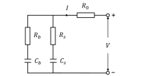
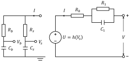
Figure 1: (a) The original double-capacitor model; (b) the proposed NDC model.

II NDC Model Development

This section develops the NDC model and presents the mathematical equations governing its dynamic behavior.

To begin with, let us review the original linear double-capacitor model proposed in [1]. As shown in Figure 1, this model includes two capacitors in parallel, $C_{b}$ and $C_{s}$, each connected with a serial resistor, $R_{b}$ and $R_{s}$, respectively. The double-capacitor structure simulates a battery’s electrode, providing storage for electric charge, and the parallel connection between them allows the transport of charge within the electrode to be described. Specifically, one can consider the $R_{s}$-$C_{s}$ circuit as corresponding to the electrode surface region exposed to the electrolyte; the $R_{b}$-$C_{b}$ circuit represents an analogy of the bulk inner part of the electrode. As such, this model has the following features:

• $C_{b}\gg C_{s}$ and $R_{b}\gg R_{s}$;

• $C_{b}$ is where the majority of the charge is stored, and $R_{b}$-$C_{b}$ accounts for low-frequency responses during charging/discharging;

• $C_{s}$ is much smaller, and its voltage changes at much faster rates than that of $C_{b}$ during charging/discharging, making $R_{s}$-$C_{s}$ responsible for high-frequency responses.

In addition, $R_{0}$ is included to embody the electrolyte resistance. This model was designed in [1] for high-power lithium-ion batteries, and its application can naturally extend to double-layer capacitors that are widely used in hybrid energy storage systems, e.g., [55].

As pointed out in [26], the linear double-capacitor model can grasp the rate capacity effect, i.e., the total charge absorbed (or released) by a battery goes down with the increase in charging (or discharging) current. To see this, just notice that the terminal voltage $V$ mainly depends on $V_{s}$ (the voltage across $C_{s}$), which changes faster than $V_{b}$ (the voltage across $C_{b}$). Thus, when the current $I$ is large, the fast rise (or decline) of $V_{s}$ will make $V$ hit the cut-off threshold earlier than when $C_{b}$ has yet to be fully charged (or discharged). Another phenomenon that can be seized is the capacity and voltage recovery effect. That is, the usable capacity and terminal voltage would increase upon the termination of discharging due to the migration of charge from $C_{b}$ to $C_{s}$. However, this model by nature is a linear system, unable to describe a defining characteristic of batteries—the nonlinear dependence of OCV on the SoC. It hence is effective only when a battery is restricted to operate conservatively within some truncated SoC range that permits a linear approximation of the SoC-OCV curve.

To overcome the above issue, the NDC model is proposed, which is shown in Figure 1. It includes two changes. The primary one is to introduce a voltage source $U$, which is a nonlinear mapping of $V_{s}$, i.e., $U=h(V_{s})$. Second, an RC circuit, $R_{1}$-$C_{1}$, is added in series to $U$. Next, let us justify the above modifications from a perspective of the SPM, a simplified electrochemical model that has recently attracted wide interest.

Figure 2 gives a schematic diagram of the SPM. The SPM represents an electrode as a single spherical particle. It describes the mass balance and diffusion of lithium ions in a particle during charging/discharging by Fick’s second law of diffusion in a spherical coordinate system [5]. If subdividing a spherical particle into two finite volumes, the bulk inner domain (core) and the near-surface domain (shell), one can simplify the diffusion of lithium ions between them as the charge transport between the capacitors of the double-capacitor model, as proven in [26]. For SPM, the terminal voltage consists of three elements: the difference in the open-circuit potential of the positive and negative electrodes, the difference in the reaction overpotential, and the voltage across the film resistance [4]. The open-circuit potential depends on the lithium-ion concentration in the surface region of the sphere, which is akin to the role of $V_{s}$ here. Therefore, it is appropriate as well as necessary to introduce a nonlinear function of $V_{s}$, i.e., $h(V_{s})$, as an analogy to the open-circuit potential. With $U=h(V_{s})$, the NDC model can correctly show the influence of the charge state on the terminal voltage, while inheriting all the capabilities of the original model.

Furthermore, the NDC model also contains an RC circuit, $R_{1}$-$C_{1}$, which, together with $R_{0}$, simulates the impedance-based part of the voltage dynamics. Here, $R_{0}$ characterizes the linear kinetic aspect of the impedance, which relates to the ohmic resistance and solid electrolyte interface (SEI) resistance [56]; $R_{1}$-$C_{1}$ accounts for the voltage transients related with the charge transfer on the electrode/electrolyte interface and the ion mass diffusion in the battery [57]. This work finds that one RC circuit can offer sufficient fidelity, though it is possible to connect more RC circuits serially with $R_{1}$-$C_{1}$ to gain better accuracy.

The dynamics of the NDC model can be expressed in the state-space form as follows:

$$[left=\empheqlbrace\,]\begin{bmatrix}\dot{V}_{b}(t)\\ \dot{V}_{s}(t)\\ \dot{V}_{1}(t)\end{bmatrix} =A\begin{bmatrix}V_{b}(t)\\ V_{s}(t)\\ V_{1}(t)\end{bmatrix}+BI(t),$$ (1a)

$$V(t) =h(V_{s}(t))-V_{1}(t)+R_{0}I(t),$$ (1b)

where

$$A=\begin{bmatrix}\frac{-1}{C_{b}(R_{b}+R_{s})}&\frac{1}{C_{b}(R_{b}+R_{s})}&0\\ \frac{1}{C_{s}(R_{b}+R_{s})}&\frac{-1}{C_{s}(R_{b}+R_{s})}&0\\ 0&0&\frac{-1}{R_{1}C_{1}}\end{bmatrix},\ B=\begin{bmatrix}\frac{R_{s}}{C_{b}(R_{b}+R_{s})}\\ \frac{R_{b}}{C_{s}(R_{b}+R_{s})}\\ \frac{-1}{C_{1}}\end{bmatrix}.$$

In above, $I>0$ for charging, $I<0$ for discharging, and $V_{1}$ refers to the voltage across the $R_{1}$-$C_{1}$ circuit. One can parameterize $h(V_{s})$ as a polynomial. A fifth-order polynomial is empirically selected here:

$$h(V_{s})=\alpha_{0}+\alpha_{1}V_{s}+\alpha_{2}V_{s}^{2}+\alpha_{3}V_{s}^{3}+\alpha_{4}V_{s}^{4}+\alpha_{5}V_{s}^{5},$$

where $\alpha_{i}$ for $i=0,1,\ldots,5$ are coefficients. Note that $h(V_{s})$ should be lower and upper bounded, depending on a battery’s operating voltage range. This implies that $V_{b}$ and $V_{s}$ must also be bounded. For any bounds selected for them, it is always possible to find out a set of coefficients $\alpha_{i}$’s to satisfy $h(\cdot)$. Hence, one can straightforwardly normalize $V_{b}$ and $V_{s}$ to let them lie between 0 V and 1 V, without loss of generality. In other words, $V_{b}=V_{s}=1$ V at full charge (${\rm SoC}=1$) and that $V_{b}=V_{s}=0$ V for full depletion (${\rm SoC}=0$). Following this setting, SoC is given by

$${\rm SoC}=\frac{Q_{a}}{Q_{t}}=\frac{C_{b}V_{b}+C_{s}V_{s}}{C_{b}+C_{s}},$$ (2)

where $Q_{t}=C_{b}+C_{s}$ denotes the total capacity, and $Q_{a}=C_{b}V_{b}+C_{s}V_{s}$ the available capacity, respectively. It is easy to verify that the SoC’s dynamics is governed by

$$\dot{\rm SoC}=\begin{bmatrix}\frac{C_{b}}{C_{b}+C_{s}}&\frac{C_{s}}{C_{b}+C_{s}}&0\end{bmatrix}\begin{bmatrix}\dot{V}_{b}\\ \dot{V}_{s}\\ \dot{V}_{1}\end{bmatrix}=\frac{1}{Q_{t}}I.$$ (3)

Meanwhile, it is worth noting that the SoC-OCV function would share the same form with $h(\cdot)$. To see this point, recall that OCV refers to the terminal voltage when the battery is at equilibrium without current load. For the NDC model, the equilibrium happens when $V_{b}=V_{s}$, $V_{1}=0$ V and $I=0$ A, and in this case, $V_{s}=\mathrm{SoC}$ according to (2), and $\mathrm{OCV}=h(V_{s})$. This suggests that ${\rm OCV}=h({\rm SoC})$. In addition, the internal resistance $R_{0}$ is also assumed to be SoC-dependent following the recommendation in [58], taking the form of

$$R_{0}=\gamma_{1}+\gamma_{2}e^{-\gamma_{3}{\rm SoC}}+\gamma_{4}e^{-\gamma_{5}{\rm(1-SoC)}}.$$ (4)

The rest of this paper will center on developing parameter identification approaches to determine the model parameters using measurement data and apply identified models to experimental datasets to evaluate their predictive accuracy.

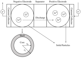
Figure 2: The single-particle model (top), and a particle (bottom) subdivided into two volumes, core and shell, which correspond to $R_{b}$-$C_{b}$ and $R_{s}$-$C_{s}$, respectively.

III Parameter Identification 1.0: Constant-Current Charging/Discharging

This section studies parameter identification for the NDC model when a constant current is applied to a battery. The discharging case is considered here without loss of generality. In a two-step procedure, the $h(\cdot)$ function is identified first, and the impedance and capacitance parameters estimated next.

III-A Identification of $h(\cdot)$

The SoC-OCV relation of the NDC model is given by ${\rm OCV}=h({\rm SoC})$, as aforementioned in Section II. Hence, one can identify $h(\cdot)$ by fitting it with a battery’s SoC-OCV data. To obtain the SoC-OCV curve, one can discharge a battery using a small current (e.g., 1/25 C-rate as suggested in [30]) from full to empty. In this process, the terminal voltage $V$ can be taken as OCV. Immediately one can see that $\alpha_{0}=\underline{V}$ and $\sum^{5}_{i=0}\alpha_{i}=\overline{V}$, where $\underline{V}$ and $\overline{V}$ are the minimum and maximum value of $V$ in the process. Therefore, ${\rm OCV}=h({\rm SoC})$ can be written as a function of $\alpha_{i}$ for $i=1,2,\ldots,4$ as follows:

$${\rm OCV}=\underline{V}+\sum^{4}_{i=1}\alpha_{i}{\rm SoC}^{i}+\left(\overline{V}-\underline{V}-\sum^{4}_{i=1}\alpha_{i}\right){\rm SoC}^{5},$$

where $\rm OCV$ can be read directly from the terminal voltage measurements. By (3), SoC can be calculated using the coulomb counting method as follows:

$${\rm SoC}=1+\frac{1}{Q_{t}}It.$$

From above, one can observe that $\alpha_{i}$ for $i=1,2,\ldots,4$ can be identified by solving a data fitting problem, which can be addressed as a linear least squares problem. The identification results are unique and can be easily obtained. Then with $\alpha_{0}=\underline{V}$ and $\alpha_{5}=\overline{V}-\underline{V}-\sum^{4}_{i=1}\alpha_{i}$, the function $h(\cdot)$ becomes explicit and ready for use.

III-B Identification of Impedance and Capacitance

Now, consider discharging the battery by a constant current of normal magnitude to determine the impedance and capacitance parameters. The identification can be attained by expressing the terminal voltage in terms of the parameters and then fitting it to the measurement data.

III-B1 Terminal Voltage Response Analysis

Consider a battery left idling for a long period of time, and then discharge it using a constant current. According to (1a), $V_{s}$ can be derived as

$$V_{s}(t) =V_{s}(0)+\frac{It}{C_{b}+C_{s}}+\frac{C_{b}(R_{b}C_{b}-R_{s}C_{s})I}{(C_{b}+C_{s})^{2}}$$

$$\quad\quad\cdot\left[1-\exp\left({-\frac{C_{b}+C_{s}}{C_{b}C_{s}(R_{b}+R_{s})}t}\right)\right],$$ (5)

where $V_{s}(0)$ is known to us as it can be accessed from $\rm{SoC}(0)$ when the battery is initially relaxed. However, it is impossible to identify $C_{b}$, $R_{b}$, $C_{s}$ and $R_{s}$ altogether. This issue can be seen from (III-B1), where $V_{s}$ depends on three parameters, i.e., $1/(C_{b}+C_{s})$, ${C_{b}(R_{b}C_{b}-R_{s}C_{s})}/{(C_{b}+C_{s})^{2}}$ and $(C_{b}+C_{s})/\left[{C_{b}C_{s}(R_{b}+R_{s})}\right]$. Even if the three parameters are known, it is still not possible to extract all the four individual impedance and capacitance parameters from them due to the parameter redundancy. Therefore, one can sensibly assume $R_{s}=0$, as recommended in [42]. This is a tenable assumption for the NDC model since $R_{s}\ll R_{b}$ as aforementioned. As a result, (III-B1) reduces to

$$V_{s}(t)=V_{s}(0)+\beta_{1}It+\beta_{2}I\left(1-e^{-\beta_{3}t}\right),$$ (6)

where

$$\beta_{1}=\frac{1}{C_{b}+C_{s}},\ \ \beta_{2}=\frac{R_{b}C_{b}^{2}}{(C_{b}+C_{s})^{2}},\ \ \beta_{3}=\frac{C_{b}+C_{s}}{C_{b}C_{s}R_{b}}.$$

Here, $\beta_{1}$ is known because $Q_{t}$ has been calibrated by coulomb counting in Section III-A. When $\beta_{2}$ and $\beta_{3}$ are also available, $C_{b}$, $C_{s}$ and $R_{b}$ can be reconstructed as follows:

$$C_{b}=\frac{\beta_{2}\beta_{3}}{\beta_{1}(\beta_{1}+\beta_{2}\beta_{3})},\ C_{s}=\frac{1}{\beta_{1}+\beta_{2}\beta_{3}},\ R_{b}=\frac{1}{\beta_{1}\beta_{3}C_{b}C_{s}}.$$

Further, in the above constant-current discharging scenario, the evolution of $V_{1}$ follows

$$V_{1}(t)=e^{-\beta_{5}t}V_{1}(0)-I\beta_{4}\left(1-e^{-\beta_{5}t}\right),$$ (7)

where

$$\beta_{4}=R_{1},\ \beta_{5}=\frac{1}{R_{1}C_{1}}.$$

Since the battery has idled for a long period prior to discharging, $V_{1}(0)$ relaxes at zero and can be removed from (7).

Then, combining (1b), (4), (6) and (7), the terminal voltage response is given by

$$V(\bm{\theta};t) =\sum_{i=0}^{5}\alpha_{i}V_{s}^{i}(\bm{\theta};t)+I\theta_{3}\left(1-e^{-\theta_{4}t}\right)+I\theta_{5}$$

$$\quad+I\theta_{6}e^{-\theta_{7}{\rm SoC}(t)}+I\theta_{8}e^{-\theta_{9}\left(1-{\rm SoC}(t)\right)}.$$ (8)

with

$${\bm{\theta}}=\left[\begin{matrix}\beta_{2}&\beta_{3}&\beta_{4}&\beta_{5}&\gamma_{1}&\gamma_{2}&\gamma_{3}&\gamma_{4}&\gamma_{5}\end{matrix}\right]^{{\top}},$$

and

$$V_{s}(\bm{\theta};t) =V_{s}(0)+{It}/Q_{t}+\theta_{1}I\left(1-e^{-\theta_{2}t}\right),$$

$${\rm SoC}(t) ={\rm SoC}(0)+It/Q_{t}.$$

III-B2 Data-Fitting-Based Identification of $\bm{\theta}$

In above, the terminal voltage $V$ is expressed in terms of $\bm{\theta}$, allowing one to identify $\bm{\theta}$ by minimizing the difference between the measured voltage and the voltage predicted by (III-B1). Hence, a data fitting problem similar to the one in Section III-A can be formulated. It should be noted that the resultant optimization will be nonlinear and nonconvex due to the presence of $h(\cdot)$. As a consequence, a numerical algorithm may get stuck in local minima and eventually give unreasonable estimates. A promising way of mitigating this challenge is to constrain the numerical optimization search within a parameter space that is believably correct. Specifically, one can roughly determine the lower and upper bounds of part or all of the parameters, set up a limited search space, and run numerical optimization within this space. With this notion, the identification problem can be formulated as a constrained optimization problem:

$$\hat{\bm{\theta}}= \arg\min_{\bm{\theta}}{1\over 2}\left[\bm{y}-{\bm{V}}(\bm{\theta})\right]^{{\top}}{\bm{Q}}^{-1}\left[\bm{y}-{\bm{V}}(\bm{\theta})\right],$$ (9a)

s.t. $$\ \underline{\bm{\theta}}\leq\bm{\theta}\leq\overline{\bm{\theta}},$$ (9b)

where $\hat{\bm{\theta}}$ is the estimate of $\bm{\theta}$, $\underline{\bm{\theta}}$ and $\overline{\bm{\theta}}$ are the pre-set lower and upper bounds of $\bm{\theta}$, respectively, $\bm{y}$ the terminal voltage measurement vector, $\bm{Q}$ an $M\times M$ symmetric positive definite matrix representing the covariance of the measurement noise, with $M$ being the number of the data points. Besides,

$${\bm{y}} =\begin{bmatrix}y(t_{1})&y(t_{2})&\cdots&y(t_{M})\end{bmatrix}^{{\top}},$$

$${\bm{V}}({\bm{\theta}}) =\begin{bmatrix}V(\bm{\theta};t_{1})&V(\bm{\theta};t_{2})&\cdots&V(\bm{\theta};t_{M})\end{bmatrix}^{{\top}}.$$

Multiple numerical algorithms are available in the literature to solve (9), a choice among which is the interior-point-based trust-region method [39].

Figure 3: The Wiener-type structure of the nonlinear double-capacitor (NDC) model.

IV Parameter Identification 2.0: Variable-Current Charging/Discharging

While it is not unusual to charge or discharge a battery at a constant current, real-world battery systems such as those in electric vehicles generally operate at variable currents. Motivated by practical utility, an interesting and challenging question is: Will it be possible to estimate all the parameters of the NDC model in one shot when an almost arbitrary current profile is applied to a battery? Having this question addressed will greatly improve the availability of the model, even to an on-demand level, for battery management tasks. This section offers a study in this regard from a Wiener identification perspective. It first unveils the NDC model’s inherent Wiener-type structure and then develops an MAP-based identification approach. Here, the study assumes $R_{0}$ to be constant for convenience.

IV-A Wiener-Type Strucutre of the NDC Model

The NDC model is structurally similar to a Wiener system—the double RC circuits constitute a linear dynamic subsystem, and cascaded with it is a nonlinear mapping. The following outlines the discrete-time Wiener-type formulation of (1).

Suppose that (1a) is sampled with a time period $\Delta T$ and then discretized by the zero-order-hold (ZOH) method. The discrete-time model is expressed as

$$x(t_{k+1})=A_{d}x(t_{k})+B_{d}I(t_{k}),$$ (10)

where $k$ is the discrete-time index with $t_{k}=k\Delta T$, and

$$A_{d}=e^{A\Delta T},\ B_{d}=\left(\int^{\Delta T}_{0}e^{A\tau}{\rm d}\tau\right)B.$$

Let us use $t$ instead of $t_{k}$ to represent the discrete time instant in sequel for notational simplicity. Then, (10) can be written as

$$x(t)=(qI_{3\times 3}-A_{d})^{-1}B_{d}I(t)+(qI_{3\times 3}-A_{d})^{-1}qx(0),$$

where $q$ is the forward shift operator, and $I_{3\times 3}\in\mathbb{R}^{3\times 3}$ is an identity matrix, respectively. Since $V_{s}(t)=\begin{bmatrix}0&1&0\end{bmatrix}x(t)$ and $V_{1}(t)=\begin{bmatrix}0&0&1\end{bmatrix}x(t)$, one can obtain the following after some lengthy derivation:

$$V_{s}(t) =G_{1}(q)I(t)+G_{2}(q)V_{s}(0),$$ (11)

$$V_{1}(t) =G_{3}(q)I(t)+G_{4}(q)V_{1}(0),$$ (12)

where

$$G_{1}(q) =\frac{(\beta_{1}+\beta_{2})q^{-1}-(\beta_{1}\beta_{3}+\beta_{2})q^{-2}}{1-(1+\beta_{3})q^{-1}+\beta_{3}q^{-2}},$$

$$G_{2}(q) =\frac{1}{1-q^{-1}},$$

$$G_{3}(q) =\frac{\beta_{4}q^{-1}}{1+\beta_{5}q^{-1}},$$

$$G_{4}(q) =\frac{1}{1+\beta_{5}q^{-1}},$$

with

$${\beta}_{1} =\frac{A_{21}B_{11}+A_{12}B_{21}}{A_{12}+A_{21}}\Delta{T},$$

$${\beta}_{2} =\frac{A_{21}(B_{21}-B_{11})}{(A_{12}+A_{21})^{2}}\left(1-\beta_{3}\right),$$

$$\beta_{3} =e^{-(A_{12}+A_{21})\Delta{T}},$$

$$\beta_{4} =-\left(\beta_{5}+1\right)B_{31}/A_{33},$$

$$\beta_{5} =-e^{A_{33}\Delta T}.$$

Note that the notation $\beta$ is slightly abused above without causing confusion. Assume that the battery has been at rest for a sufficiently long time to achieve an equilibrium state before a test. In this setting, $V_{s}(0)={\rm SoC}(0)$, $V_{1}(0)=0\leavevmode\nobreak\ \rm V$, and $G_{4}(q)V_{1}(0)=0$. Besides, one can also see that the same parameter redundancy issue as in Section III-B occurs again—only three parameters, $\beta_{1}$ through $\beta_{3}$, appear in (11), but four physical parameters, $C_{b}$, $C_{s}$, $R_{b}$ and $R_{s}$, need to be identified. To fix this, let $R_{s}=0$ as was done before. Then $\beta_{1}$ through $\beta_{3}$ reduce to be

$${\beta}_{1}=\frac{\Delta T}{C_{b}+C_{s}},\ {\beta}_{2}=\frac{R_{b}C_{b}^{2}\left(1-{\beta}_{3}\right)}{(C_{b}+C_{s})^{2}},\ {\beta}_{3}=e^{-\frac{C_{b}+C_{s}}{C_{b}C_{s}R_{b}}\Delta{T}}.$$

If $\beta_{1}$ through $\beta_{5}$ become available, the physical parameters can be reconstructed as follows:

$$C_{b} =\frac{\Delta{T}}{{\beta}_{1}}-C_{s},\ C_{s}=\frac{\left(1-{\beta}_{3}\right)\Delta T}{{\beta}_{1}-{\beta}_{1}{\beta}_{3}-{\beta}_{2}{\rm log}{\beta}_{3}},$$

$$R_{b} =-\frac{\left(\Delta T\right)^{2}}{C_{b}C_{s}{\beta}_{1}{\rm log}{\beta}_{3}},\ R_{1}=\frac{-\beta_{4}}{\beta_{5}+1},\ C_{1}=\frac{-\Delta T}{{\rm log}(-\beta_{5})R_{1}}.$$

Finally, it is obvious that

$$V(t)=h\left[G_{1}(q)I(t)+G_{2}(q)V_{s}(0)\right]-G_{3}(q)I(t)+R_{0}I(t).$$ (13)

The above equation reveals the block-oriented Wiener-type structure of the NDC model, as depicted in Figure 3, in which the linear dynamic model $G_{1}(q)$ and the nonlinear function $h(V_{s})$ are interconnected sequentially. Given (13), the next pursuit is to estimate all of the parameters simultaneously, which include $\alpha_{i}$ for $i=1,2,\dots,4$, ${\beta}_{i}$ for $i=1,2,\dots,5$, and $R_{0}$. Here, $\alpha_{0}$ and $\alpha_{5}$ are free of identification as they can be expressed by $\alpha_{i}$ for $i=1,2,\dots,4$ (see Section III-A).

IV-B MAP-Based Wiener Identification

Consider the following model based on (13) for notational convenience:

$$z(t) =V(\bm{\theta};u(t))+v(t),$$ (14)

where $u$ is the input current $I$, $z$ the measured voltage, $v$ the measurement noise added to $V$ and assumed to follow a Gaussian distribution $\mathcal{N}(0,\sigma^{2})$, and

$$V(\bm{\theta};u(t)) =h\left[G_{1}(q,\bm{\theta})u(t)+G_{2}(q)V_{s}(0),\bm{\theta}\right]$$

$$\quad-G_{3}(q,\bm{\theta})u(t)+\theta_{10}u(t),$$

with

$$\bm{\theta}=\begin{bmatrix}\alpha_{1}&\alpha_{2}&\alpha_{3}&\alpha_{4}&\beta_{1}&\beta_{2}&\beta_{3}&\beta_{4}&\beta_{5}&R_{0}\end{bmatrix}^{{\top}}.$$

The input and output datasets are denoted as

$${\bm{u}} =\begin{bmatrix}u(t_{1})&u(t_{2})&\cdots&u(t_{N})\end{bmatrix}^{{\top}}\in\mathbb{R}^{N\times 1},$$

$${\bm{z}} =\begin{bmatrix}z(t_{1})&z(t_{2})&\cdots&z(t_{N})\end{bmatrix}^{{\top}}\in\mathbb{R}^{N\times 1},$$

where $N$ is the total number of data samples. A combination of them is expressed as

$${\bm{Z}}=\begin{bmatrix}{\bm{u}}&{\bm{z}}\end{bmatrix}.$$

An ML-based approach is developed in [53] to deal with Wiener system identification. If applied to (14), it leads to consideration of the following problem:

$$\hat{\bm{\theta}} ={\rm arg}\max_{\bm{\theta}}p(\bm{Z}|\bm{\theta}).$$

Following this line, one can derive a likelihood cost function and perform minimization to find out $\hat{\bm{\theta}}$. However, this method can be vulnerable to the risk of local minima because of the nonconvexity issue resulting from the static nonlinear function $h(\cdot)$. This can cause unphysical estimates. While carefully selecting an initial guess is suggested to alleviate this problem [59], it is often found inadequate for many practical systems. In particular, our study showed that it could hardly deliver reliable parameter estimation when used to handle the NDC model identification.

MAP-based Wiener identification thus is proposed here to overcome this problem. The MAP estimation can incorporate some prior knowledge about parameters to help drive the parameter search toward a reasonable minimum point. Specifically, consider maximizing the a posteriori probability distribution of $\bm{\theta}$ conditioned on $\bm{Z}$:

$$\hat{\bm{\theta}}={\rm arg}\max_{\bm{\theta}}p(\bm{\theta}|\bm{Z}).$$ (15)

By the Bayes’ theorem, it follows that

$$p(\bm{\theta}|\bm{Z})=\frac{p(\bm{Z}|\bm{\theta})\cdot p(\bm{\theta})}{p(\bm{Z})}\propto p(\bm{Z}|\bm{\theta})\cdot p(\bm{\theta}).$$

In above, $p(\bm{\theta})$ quantifies the prior information available about $\bm{\theta}$. A general way is to characterize it as a Gaussian random vector following the distribution $p(\bm{\theta})\sim\mathcal{N}\left(\bm{m},{\bm{P}}\right)$. Based on (14), $p(\bm{z}|\bm{\theta})\sim\mathcal{N}\left(\bm{V}(\bm{\theta};\bm{u}),{\bm{R}}\right)$, where $\bm{R}=\sigma^{2}\bm{I}$ and

$$\bm{V}(\bm{\theta};\bm{u}) =\begin{bmatrix}V(\bm{\theta};u(t_{1}))&\cdots&V(\bm{\theta};u(t_{N}))\end{bmatrix}^{{\top}}.$$

Then,

$$p(\bm{Z}|\bm{\theta})\cdot p(\bm{\theta})$$

$$\quad\propto{\rm exp}\bigg{(}-\frac{1}{2}\left[\bm{z}-{\bm{V}}\left(\bm{\theta};\bm{u}\right)\right]^{{\top}}\bm{R}^{-1}\left[\bm{z}-{\bm{V}}\left(\bm{\theta};\bm{u}\right)\right]\bigg{)}$$

$$\quad\quad\ \cdot{\rm exp}\left(-\frac{1}{2}\left(\bm{\theta}-\bm{m}\right)^{{\top}}{\bm{P}}^{-1}\left(\bm{\theta}-\bm{m}\right)\right).$$

If using the log-likelihood, the problem in (15) is equivalent to

$$\hat{\bm{\theta}}={\rm arg}\min_{\bm{\theta}}J(\bm{\theta}),$$ (16)

where

$$J(\bm{\theta}) =\frac{1}{2}\left[\bm{z}-{\bm{V}}\left(\bm{\theta};\bm{u}\right)\right]^{{\top}}\bm{R}^{-1}\left[\bm{z}-{\bm{V}}\left(\bm{\theta};\bm{u}\right)\right]$$

$$\quad+\frac{1}{2}\left(\bm{\theta}-\bm{m}\right)^{{\top}}\bm{P}^{-1}\left(\bm{\theta}-\bm{m}\right).$$

For the nonlinear optimization problem in (16), one can exploit the quasi-Newton method to numerically solve it [53]. This method iteratively updates the parameter estimate through

$$\bm{\theta}_{k+1}=\bm{\theta}_{k}+\lambda_{k}\bm{s}_{k}.$$ (17)

Here, $\lambda_{k}$ denotes the step size at iteration step $k$, and $\bm{s}_{k}$ is the gradient-based search direction given by

$$\bm{s}_{k}=-\bm{B}_{k}\bm{g}_{k},$$ (18)

where $\bm{B}_{k}\in\mathbb{R}^{10\times 10}$ is a positive definite matrix that approximates the Hessian matrix $\nabla^{2}J\left(\bm{\theta}_{k}\right)$, and $\bm{g}_{k}=\nabla J\left(\bm{\theta}_{k}\right)\in\mathbb{R}^{10\times 1}$. Based on the well-known BFGS update strategy [60], $\bm{B}_{k}$ can be updated by

$$\bm{B}_{k}=\left(\bm{I}-\frac{\bm{\delta}_{k}\bm{\gamma}_{k}^{{\top}}}{\bm{\delta}_{k}^{{\top}}\bm{\gamma}_{k}}\right)\bm{B}_{k-1}\left(\bm{I}-\frac{\bm{\gamma}_{k}\bm{\delta}_{k}^{{\top}}}{\bm{\delta}_{k}^{{\top}}\bm{\gamma}_{k}}\right)+\frac{\bm{\delta}_{k}\bm{\delta}_{k}^{{\top}}}{\bm{\delta}_{k}^{{\top}}\bm{\gamma}_{k}},$$ (19)

with $\bm{\delta}_{k}=\bm{\theta}_{k}-\bm{\theta}_{k-1}$ and $\bm{\gamma}_{k}=\bm{g}_{k}-\bm{g}_{k-1}$. In addition,

$$\bm{g}_{k} =-\left(\frac{\partial{\bm{V}}\left(\bm{\theta}_{k};\bm{u}\right)}{\partial\bm{\theta}_{k}}\right)^{{\top}}\bm{R}^{-1}\left[\bm{z}-\bm{V}\left(\bm{\theta}_{k};\bm{u}\right)\right]$$

$$\quad+\bm{P}^{-1}\left(\bm{\theta}_{k}-\bm{m}\right),$$ (20)

where each column of $\frac{\partial{\bm{V}}\left(\bm{\theta};\bm{u}\right)}{\partial\bm{\theta}}\in\mathbb{R}^{N\times 10}$ is given by

$$\frac{\partial{\bm{V}}\left(\bm{\theta};\bm{u}\right)}{\partial\theta_{i}} =\bm{x}^{\circ i}-\bm{x}^{\circ 5}\leavevmode\nobreak\ {\rm for}\leavevmode\nobreak\ i=1,2,\dots,4,$$

$$\frac{\partial{\bm{V}}\left(\bm{\theta};\bm{u}\right)}{\partial\theta_{5}} =\bm{\Sigma}\circ\frac{q^{-1}-\theta_{7}q^{-2}}{1-(1+\theta_{7})q^{-1}+\theta_{7}q^{-2}}\bm{u},$$

$$\frac{\partial{\bm{V}}\left(\bm{\theta};\bm{u}\right)}{\partial\theta_{6}} =\bm{\Sigma}\circ\frac{q^{-1}-q^{-2}}{1-(1+\theta_{7})q^{-1}+\theta_{7}q^{-2}}\bm{u},$$

$$\frac{\partial{\bm{V}}\left(\bm{\theta};\bm{u}\right)}{\partial\theta_{7}} =\bm{\Sigma}\circ\frac{\theta_{6}q^{-2}-2\theta_{6}q^{-3}+\theta_{6}q^{-4}}{\left(1-(1+\theta_{7})q^{-1}+\theta_{7}q^{-2}\right)^{2}}\bm{u},$$

$$\frac{\partial{\bm{V}}\left(\bm{\theta};\bm{u}\right)}{\partial\theta_{8}} =\frac{-q^{-1}}{1+\theta_{9}q^{-1}}\bm{u},$$

$$\frac{\partial{\bm{V}}\left(\bm{\theta};\bm{u}\right)}{\partial\theta_{9}} =\frac{\theta_{8}q^{-2}}{1+2\theta_{9}q^{-1}+\theta_{9}^{2}q^{-2}}\bm{u},$$

$$\frac{\partial{\bm{V}}\left(\bm{\theta};\bm{u}\right)}{\partial\theta_{10}} =\bm{u},$$

with

$$\bm{x} =G_{1}(q,\bm{\theta})\bm{u}+G_{2}(q)V_{s}(0)\bm{1},$$

$$\bm{\Sigma} =\sum^{4}_{i=1}i\theta_{i}{\bm{x}}^{\circ(i-1)}+5\left(\overline{V}-\underline{V}-\sum^{4}_{i=1}\theta_{i}\right)\bm{x}^{\circ 4}.$$

Here, $\bm{x}\circ\bm{u}$ denotes the Hadamard product of $\bm{x}$ and $\bm{u}$, $\bm{x}^{\circ 2}$ denotes the Hadamard power with $\bm{x}^{\circ 2}=\bm{x}\circ\bm{x}$, and $\bm{1}\in\mathbb{R}^{N\times 1}$ denotes a column vector with all elements equal to one.

Finally, note that $\lambda_{k}$ needs to be chosen carefully to make $J(\bm{\theta})$ decrease monotonically. One can use the Wolfe conditions and let $\lambda_{k}$ be selected such that

$${J}\left(\bm{\theta}_{k}+\lambda_{k}\bm{s}_{k}\right) \leq{J}\left(\bm{\theta}_{k}\right)+c_{1}\lambda_{k}\bm{g}_{k}^{{\top}}\bm{s}_{k},$$ (21a)

$$\nabla J\left(\bm{\theta}_{k}+\lambda_{k}\bm{s}_{k}\right)^{{\top}}\bm{s}_{k} \geq c_{2}\nabla J\left(\bm{\theta}_{k}\right)^{{\top}}\bm{s}_{k},$$ (21b)

with $0<c_{1}<c_{2}<1$. For the quasi-Newton method, $c_{1}$ is usually set to be quite small, e.g., $c_{1}=10^{-6}$, and $c_{2}$ is typically set to be 0.9. The selection of $\lambda_{k}$ can be based on trial and error in implementation. One can start with picking a number and check the Wolfe conditions. If the conditions are not satisfied, reduce the number and check again. An interested reader is referred to [60] for detailed discussion about the $\lambda_{k}$ selection. Summarizing the above, Table I outlines the implementation procedure for the MAP-based Wiener identification.

Table I: Quasi-Newton-based implementation for MAP-based Wiener identification.

  Initialize $\bm{\theta}_{0}$ and set the convergence tolerance   repeat       Compute $\bm{g}_{k}$ via (IV-B)      if $k=0$ then         Initialize $\bm{B}_{0}=0.001\frac{1}{\lVert{\bm{g}_{0}}\rVert}\bm{I}$      else         Compute $\bm{B}_{k}$ via (19)      end if      Compute $\bm{s}_{k}$ via (18)      Find $\lambda_{k}$ that satisfies the Wolfe conditions (21)      Perform the update via (17)   until ${J}(\bm{\theta}_{k})$ converges   return  $\hat{\bm{\theta}}=\bm{\theta}_{k}$

Remark 1

While the MAP estimation has enjoyed a long history of addressing a variety of estimation problems, no study has been reported about its application to Wiener system identification to our knowledge. Here, it is found to be a very useful approach for providing physically reasonable parameter estimation for practical systems, as it takes into account some prior knowledge about the unknown parameters. In a Gaussian setting as adopted here, the prior $p(\bm{\theta})$ translates into a regularization term in $J(\bm{\theta})$, which prevents incorrect fitting and enhances the robustness of the numerical optimization against nonconvexity.

Remark 2

The proposed 2.0 identification approach requires some prior knowledge of the parameters to be available, which can be developed in several ways in practice. First, $R_{0}$ can be roughly estimated using the voltage drop at the beginning of the discharge, to which it is a main contributor. Second, the polynomial coefficients of $h(\cdot)$ can be approximately obtained from an experimentally calibrated SoC-OCV curve if there is any. Third, one can derive a rough range for $C_{b}+C_{s}$ if a battery’s capacity is approximately known. Finally, as the parameters of batteries of the same kind and brand are usually close, one can take the parameter estimates acquired from one battery as prior knowledge for another.

Remark 3

In general, a prerequisite for successful identification is that the parameters must be identifiable in a certain sense. Following along similar lines as in [18, 61], one can rigorously define the parameters’ local identifiability for the considered Wiener identification problem and find out that a sufficient condition for it to hold is the full rankness of the sensitivity matrix ${\partial{\bm{V}}\left(\bm{\theta};\bm{u}\right)}/{\partial\bm{\theta}}$, which can be used for identifiability testing. Using this idea, our simulations consistently showed the full rankness of the sensitivity matrix under variable current profiles such as those in Figure 8, indicating that the NDC model can be locally identifiable. Related with identification is optimal input design, which concerns designing the best current profile to maximize the parameter identifiability [50, 51]. It will be part of our future research to explore this interesting problem for the NDC model.

Remark 4

It is worth mentioning that the 2.0 identification approach can be readily extended to identify some other ECMs that have a Wiener-like structure like the Rint and Thevenin models. One can follow similar lines to develop the computational procedures for each, and hence the details are skipped here.

Remark 5

The 1.0 and 2.0 identification approaches are designed to perform offline identification for the NDC model, each with its own advantages. The 1.0 approach is designed for in-lab battery modeling and analysis, using simple two-step (trickle- and constant-current discharging) battery testing protocols. While requiring a long time for experiments, it can offer high accuracy in parameter estimation. More sophisticated by design, the 2.0 approach can extract the parameters all at once from data based on variable current profiles. It can be conveniently exploited to determine the NDC model for batteries operating in real-world applications.

V Experimental Validation

This section presents experimental validation of the proposed NDC model and parameter identification 1.0 and 2.0 approaches. All the experiments in this section were conducted on a PEC^® SBT4050 battery tester (see Figure 4). It can support charging/discharging with arbitrary current-, voltage- and power-based loads (up to 40 V and 50 A). A specialized server is used to prepare and configure a test offline and collect experimental data online via the associated software LifeTest^TM. Using this facility, charging/discharging tests were performed to generate data on a Panasonic NCR18650B lithium-ion battery cell, which was set to operate between 3.2 V (fully discharged) and 4.2 V (fully charged).

V-A Validation Based on Parameter Identification 1.0

This validation first extracts the NDC model from training dataset using the 1.0 identification approach in Section III and then applies the identified model to validation datasets to assess its predictive capability.

As a first step, the cell was fully charged and relaxed for a long time period. Then, a full discharge test was applied to the cell using a trickle constant current of 0.1 A (about 1/30 C-rate). With this test, the total capacity is determined to be $Q_{t}=3.06\leavevmode\nobreak\ {\rm Ah}$ by coulomb counting, implying $C_{b}+C_{s}=11,011\leavevmode\nobreak\ \rm F$. Further, from the SoC-OCV curve fitting, we obtain

$${\rm OCV}= \leavevmode\nobreak\ 3.2+2.59\cdot{\rm SoC}-9.003\cdot{\rm SoC}^{2}+18.87\cdot{\rm SoC}^{3}$$

$$-17.82\cdot{\rm SoC}^{4}+6.325\cdot{\rm SoC}^{5},$$

which establishes $h(\cdot)$ immediately. The measured and identified SoC-OCV curves are compared in Figure 5. Next, the cell was fully charged again and left idling for a long time. This was then followed by a full discharge using a constant current of 3 A to produce data for estimation of the impedance and capacitance parameters. The identification was achieved by solving the constrained optimization problem in (9). The computation took around 1 sec, performed on a Dell Precision Tower 3620 equipped with 3 GHz Inter Xeon CPU, 16 Gb RAM and MATLAB R2018b. Table II summarizes the initial guess, lower and upper bounds, and obtained estimates of the parameters. The physical parameter estimates are extracted as: $C_{b}=10,037\leavevmode\nobreak\ {\rm F}$, $C_{s}=973\leavevmode\nobreak\ {\rm F}$, $R_{b}=0.019\leavevmode\nobreak\ \rm{\Omega}$, $R_{s}=0$, $R_{1}=0.02\leavevmode\nobreak\ \rm{\Omega}$, $C_{1}=3,250\leavevmode\nobreak\ \rm F$, and

$$R_{0}=0.0531+0.1077e^{-3.807\cdot{\rm SoC}}+0.0533e^{-7.613\cdot{\rm(1-SoC)}}.$$

The model is now fully available from the two steps. Figure 6 shows that it accurately fits with the measurement data.

Figure 4: PEC^® SBT4050 battery tester.

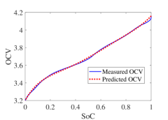
Figure 5: Identification 1.0: parameter identification of $h(\cdot)$ that defines SoC-OCV relation.

Table II: Identification 1.0: initial guess, bound limits and identification results.

Name	$\beta_{2}$	$\beta_{3}$	$\beta_{4}$	$\beta_{5}$	$\gamma_{1}$	$\gamma_{2}$	$\gamma_{3}$	$\gamma_{4}$	$\gamma_{5}$
Initial guess	0.02	0.05	0.005	1/100	0.05	0.2	8	0.07	12
${\underline{\bm{\theta}}}$	0.005	0.005	0.001	1/800	0.01	0.05	1	0.01	1
${\overline{\bm{\theta}}}$	0.2	0.2	0.03	1/10	0.09	0.35	15	0.12	15
$\hat{\bm{\theta}}$	0.0163	0.0575	0.02	1/65	0.0531	0.1077	3.807	0.0533	7.613

• Note: quantities are given in SI standard units in Tables II and III.

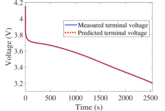
Figure 6: Identification 1.0: model fitting with the training data obtained under 3 A constant-current discharging.

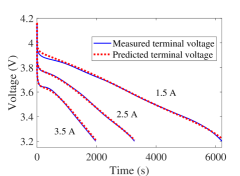
Figure 7: Identification 1.0: predictive fitting over validation data obtained by discharging at different constant currents.

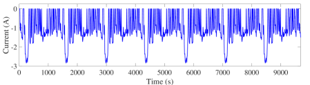
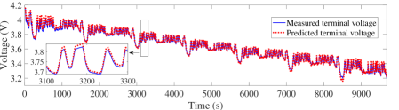
Figure 8: Identification 1.0: predictive fitting over validation dataset obtained by discharging at varying currents (0$\sim$3 A). (a) Current profile. (b) Voltage fitting.

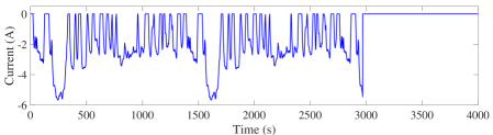
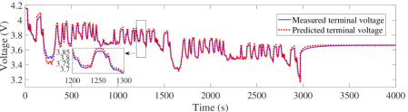
Figure 9: Identification 1.0: predictive fitting over validation dataset obtained by discharging at varying currents ($0\sim 6$ A). (a) Current profile. (b) Voltage fitting.

While an identified model generally can well fit a training dataset, it is more meaningful and revealing to examine its predictive performance on some different datasets. Hence, five more tests were conducted by discharging the cell using constant currents of 1.5 A, 2.5 A and 3.5 A and two variable current profiles, respectively. Figure 7 shows what the identified model predicts for discharging at constant currents. An overall high accuracy is observed, even though the prediction is slightly less accurate when the current is 1.5 A, probably because the parameters are current-dependent to a certain extent. The variable current profiles are portrayed in Figures 8 and 9, which were created by scaling the Urban Dynamometer Driving Schedule (UDDS) profile in [62] to span the ranges of $0$$\sim$$3$ A and $0$$\sim$$6$ A, respectively. Figures 8 and 9 present the predictive fitting results. Both of them illustrate that the model-based voltage prediction is quite close to the actual measurements. These results demonstrate the excellent predictive capability of the NDC model.

V-B Validation Based on Parameter Identification 2.0

Table III: Identification 2.0: initial guess, prior knowledge and identification results.

Name	$\alpha_{1}$	$\alpha_{2}$	$\alpha_{3}$	$\alpha_{4}$	$\breve{\beta}_{1}$	$\breve{\beta}_{2}$	$\breve{\beta}_{3}$	$\beta_{4}$	$\beta_{5}$	$R_{0}$
Initial guess	2.59	-9.003	18.87	-17.82	$9.078\times 10^{-5}$	$8.914\times 10^{-4}$	0.964	$-4.938\times 10^{-4}$	$-0.9753$	0.08
$\bm{m}$	-	-	-	-	$9.078\times 10^{-5}$	$8.914\times 10^{-4}$	0.964	$-4.938\times 10^{-4}$	$-0.9753$	0.08
$\sqrt{{\rm diag}(\bm{P})}$	-	-	-	-	$0.001\times m_{5}$	$0.15\times m_{6}$	$0.15\times m_{7}$	$0.15\times m_{8}$	$0.15\times m_{9}$	$0.15\times m_{10}$
$\hat{\bm{\theta}}$	2.32	-8.15	19.345	-20.78	$9.082\times 10^{-5}$	$9.227\times 10^{-4}$	0.982	$-4.859\times 10^{-4}$	$-0.8153$	0.069

Let us now consider the 2.0 identification approach developed in Section III, which treats the NDC model as a Wiener-type system and performs MAP-based parameter estimation. This approach advantageously allows all the parameters to be estimated in a convenient one-shot procedure.

Following the manner in Section V-A, one can apply the 2.0 approach to a training dataset to extract an NDC model and then use it to predict the responses over several other different datasets. The validation here is also set to evaluate the NDC model against the Rint model [12] and the Thevenin model with one serial RC circuit [12], which are commonly used in the literature. The comparison also extends to a basic version of the NDC model (referred to as “basic NDC” in sequel), one with a constant $R_{0}$ and without $R_{1}$-$C_{1}$ circuit, with the purpose of examining the utility of the NDC model when it is reduced to a simpler form. Note that, even though the NDC model is the most sophisticated among them, all of the four models offer high computational efficiency by requiring only a small number of arithmetic operations.

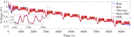
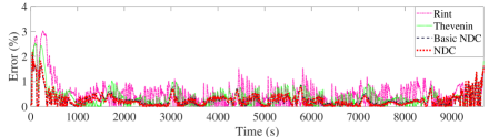
Figure 10: Identification 2.0. (a) Model fitting with training dataset. (b) Fitting error in percentage.

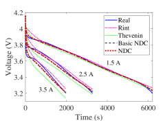
Figure 11: Identification 2.0: predictive fitting over validation datasets obtained by discharging at different varying currents.

These four models are all Wiener-type, so the 2.0 identification approach can be used to identify them on the same training dataset, i.e., the one shown in Figure 8, thus ensuring a fair comparison. The parameter setting for the NDC model identification and the estimation result are summarized in Table III. The computation took around 4 sec. The resultant physical parameter estimates are given by: $C_{b}=10,031\leavevmode\nobreak\ {\rm F}$, $C_{s}=979\leavevmode\nobreak\ {\rm F}$, $R_{b}=0.063\leavevmode\nobreak\ \rm{\Omega}$, $R_{s}=0$, $R_{1}=0.003\leavevmode\nobreak\ \rm{\Omega}$, $C_{1}=2,449\leavevmode\nobreak\ \rm F$ and $R_{0}=0.069\leavevmode\nobreak\ \rm\Omega$. The identification results for the Rint, Thevenin model and basic NDC models are omitted here for the sake of space.

Figure 10 depicts how the identified models fit with the training dataset. One can observe that the NDC model and its basic version show excellent fitting accuracy, overall better than the Rint and Thevenin models. A more detailed comparison is given in Figure 10, which displays the fitting error in percentage. It is seen that the Rint model shows the least accuracy, followed by the Thevenin model. The NDC model and its basic version well outperform them, with the NDC model performing slightly better.

Proceeding forward, let us investigate the predictive performance of the four models over several validation datasets. First, consider the datasets obtained by constant-current discharging at 1.5 A, 2.5 A and 3.5 A, as illustrated in Figure 7. Figure 11 demonstrates that the NDC model and its basic version can predict the voltage responses under different currents much more accurately than the Rint and Thevenin models. Next, consider the dataset in Figure 9 based on variable-current discharging. Figure 12 shows that the prediction accuracy of all the models is lower than the fitting accuracy, which is understandable. However, the NDC model and its basic version are still again the most capable of predicting, with the error mostly lying below $1\%$. As a contrast, while the Thevenin model can offer a decent fit with the training dataset as shown in Figure 10, its prediction accuracy over the validation dataset is not as satisfactory. This implies that it is less predictive than the NDC model.

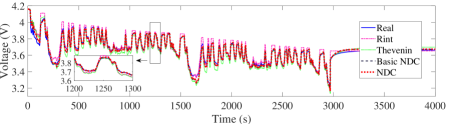
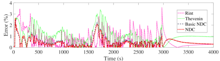
Figure 12: Identification 2.0. (a) Predictive fitting over validation dataset obtained by discharging at varying currents between 0 A and 6 A. (b) Predictive fitting error in percentage.

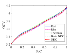
Figure 13: Identification 2.0: identification of the SoC-OCV relation based on different models, compared to the truth.

Another evaluation of interest is about the SoC-OCV relation. As mentioned earlier, the 2.0 approach can estimate all the parameters, including the function $h(\cdot)$. This allows one to write the SoC-OCV function directly based on the identified $h(\cdot)$ as it also characterizes the SoC-OCV relation. That is,

$${\rm OCV} =3.2+2.32\cdot{\rm SoC}-8.15\cdot{\rm SoC}^{2}+19.345\cdot{\rm SoC}^{3}$$

$$\quad-20.78\cdot{\rm SoC}^{4}+8.222\cdot{\rm SoC}^{5}.$$

Identification of the other three models can also lead to estimation of this function. Figure 13 compares them with the benchmark shown in Figure 5, which is obtained experimentally by discharging the cell using a small current of 0.1 A. It is obvious that the SoC-OCV curves obtained in the identification of the NDC model and its basic version are closer to the benchmark overall. This further shows the benefit of the NDC model as well as the efficacy of the 2.0 approach.

Summing up the above validation results, one can draw the following observations:

• The NDC model is the most competent among the four considered models for grasping and predicting a battery’s dynamic behavior, justifying its validity and soundness.

• The basic NDC model can offer fitting and prediction accuracy almost comparable to that of the full model. It thus can be well qualified if a practitioner wants to use a simpler NDC model yet without much loss of accuracy.

• The 2.0 identification approach is effective in estimating all the parameters of the NDC model as well as the Rint and Thevenin models in one shot from variable-current-based data profiles. It can not only ease the cost of identification considerably but also provide on-demand model availability potentially in practice.

VI Conclusion

The growing importance of real-time battery management has imposed a pressing demand for battery models with high fidelity and low complexity, making ECMs a popular choice in this field. The double-capacitor model is emerging as a favorable ECM for diverse applications, promising several advantages in capturing a battery’s dynamics. However, its linear structure intrinsically hinders a characterization of a battery’s nonlinear phenomena. To thoroughly improve this model, this paper proposed to modify its original structure by adding a nonlinear-mapping-based voltage source and a serial RC circuit. This development was justified through an analogous comparison with the SPM. Furthermore, two offline parameter estimation approaches, which were named 1.0 and 2.0, respectively, were designed to identify the model from current/voltage data. The 1.0 approach considers the constant-current charging/discharging scenarios, determining the SoC-OCV relation first and then estimating the impedance and capacitance parameters. With the observation that the NDC model has a Wiener-type structure, the 2.0 approach was derived from the Wiener perspective. As the first of its kind, it leverages the notion of MAP to address the issue of local minima that may reduce or damage the performance of the nonlinear Wiener system identification. It well lends itself to the variable-current charging/discharging scenarios and can desirably estimate all the parameters in one shot. The experimental evaluation demonstrated that the NDC model outperformed the popularly used Rint and Thevenin models in predicting a battery’s behavior, in addition to showing the effectiveness of the identification approaches for extracting parameters. Our future work will include: 1) enhancing the NDC model further to account for the effects of temperature and include the voltage hysteresis, 2) investigating optimal input design for the model, and 3) building new battery estimation and control designs based on the model.

Ning Tian received the B.Eng. and M.Sc. degrees in thermal engineering from Northwestern Polytechnic University, Xi’an, China, in 2012 and 2015. Currently, he is a Ph.D. candidate at the University of Kansas, Lawrence, KS, USA. His research interests include control theory and its application to advanced battery management.

Huazhen Fang (M’14) received the B.Eng. degree in computer science and technology from Northwestern Polytechnic University, Xi’an, China, in 2006, the M.Sc. degree in mechanical engineering from the University of Saskatchewan, Saskatoon, SK, Canada, in 2009, and the Ph.D. degree in mechanical engineering from the University of California, San Diego, CA, USA, in 2014. He is currently an Assistant Professor of Mechanical Engineering with the University of Kansas, Lawrence, KS, USA. His research interests include control and estimation theory with application to energy management, cooperative robotics, and system prognostics. Dr. Fang received the 2019 National Science Foundation CAREER Award and the awards of Outstanding Reviewer or Reviewers of the Year from Automatica, IEEE Transactions on Cybernetics, and ASME Journal of Dynamic Systems, Measurement and Control.

Jian Chen (M’06-SM’10) received the B.E. degree in measurement and control technology and instruments and the M.E. degree in control science and engineering from Zhejiang University, Hangzhou, China, in 1998 and 2001, respectively, and the Ph.D. degree in electrical engineering from Clemson University, Clemson, SC, USA, in 2005. He was a Research Fellow with the University of Michigan, Ann Arbor, MI, USA, from 2006 to 2008, where he was involved in fuel cell modeling and control. In 2013, he joined the Department of Control Science and Engineering, Zhejiang University, where he is currently a Professor with the College of Control Science and Engineering. His research interests include modeling and control of fuel cell systems, vehicle control and intelligence, machine vision, and nonlinear control.

Yebin Wang (M’10-SM’16) received the B.Eng. degree in Mechatronics Engineering from Zhejiang University, Hangzhou, China, in 1997, M.Eng. degree in Control Theory & Control Engineering from Tsinghua University, Beijing, China, in 2001, and Ph.D. in Electrical Engineering from the University of Alberta, Edmonton, Canada, in 2008. Dr. Wang has been with Mitsubishi Electric Research Laboratories in Cambridge, MA, USA, since 2009, and now is a Senior Principal Research Scientist. From 2001 to 2003 he was a Software Engineer, Project Manager, and Manager of R&D Dept. in industries, Beijing, China. His research interests include nonlinear control and estimation, optimal control, adaptive systems and their applications including mechatronic systems.

References

- [1] V. H. Johnson and A. A. Pesaran, “Temperature-dependent battery models for high-power lithium-lon batteries,” National Renewable Energy Laboratory, Tech. Rep. NREL/CP-540-28716, 2000.
- [2] M. Doyle, T. F. Fuller, and J. Newman, “Modeling of galvanostatic charge and discharge of the lithium/polymer/insertion cell,” Journal of The Electrochemical Society, vol. 140, no. 6, pp. 1526–1533, 1993.
- [3] J. C. Forman, S. J. Moura, J. L. Stein, and H. K. Fathy, “Genetic identification and fisher identifiability analysis of the Doyle–Fuller–Newman model from experimental cycling of a LiFePO4 cell,” Journal of Power Sources, vol. 210, pp. 263 – 275, 2012.
- [4] N. Chaturvedi, R. Klein, J. Christensen, J. Ahmed, and A. Kojic, “Algorithms for advanced battery-management systems,” IEEE Control Systems Magazine, vol. 30, no. 3, pp. 49–68, 2010.
- [5] M. Guo, G. Sikha, and R. E. White, “Single-particle model for a lithium-ion cell: Thermal behavior,” Journal of The Electrochemical Society, vol. 158, no. 2, pp. A122–A132, 2011.
- [6] P. W. C. Northrop, B. Suthar, V. Ramadesigan, S. Santhanagopalan, R. D. Braatz, and V. R. Subramanian, “Efficient simulation and reformulation of lithium-ion battery models for enabling electric transportation,” Journal of The Electrochemical Society, vol. 161, no. 8, pp. E3149–E3157, 2014.
- [7] C. Zou, C. Manzie, and D. Nešić, “A framework for simplification of PDE-based lithium-ion battery models,” IEEE Transactions on Control Systems Technology, vol. 24, no. 5, pp. 1594–1609, 2016.
- [8] X. Hu, D. Cao, and B. Egardt, “Condition monitoring in advanced battery management systems: Moving horizon estimation using a reduced electrochemical model,” IEEE/ASME Transactions on Mechatronics, vol. 23, no. 1, pp. 167–178, 2018.
- [9] J. E. B. Randles, “Kinetics of rapid electrode reactions,” Discussions of the Faraday Society, vol. 1, pp. 11–19, Mar. 1947.
- [10] A. I. Zia and S. C. Mukhopadhyay, Impedance Spectroscopy and Experimental Setup. Cham, Switzerland: Springer International Publishing, 2016, pp. 21–37.
- [11] S. M. G. and M. Nikdel, “Various battery models for various simulation studies and applications,” Renewable and Sustainable Energy Reviews, vol. 32, pp. 477–485, 2014.
- [12] H. He, R. Xiong, and J. Fan, “Evaluation of lithium-ion battery equivalent circuit models for state of charge estimation by an experimental approach,” Energies, vol. 4, pp. 582–598, 2011.
- [13] G. L. Plett, Battery Management Systems, Volume 1: Battery Modeling. Artech House, 2015.
- [14] C. Weng, J. Sun, and H. Peng, “A unified open-circuit-voltage model of lithium-ion batteries for state-of-charge estimation and state-of-health monitoring,” Journal of Power Sources, vol. 258, pp. 228–237, 2014.
- [15] X. Lin, H. E. Perez, S. Mohan, J. B. Siegel, A. G. Stefanopoulou, Y. Ding, and M. P. Castanier, “A lumped-parameter electro-thermal model for cylindrical batteries,” Journal of Power Sources, vol. 257, pp. 1–11, 2014.
- [16] M. Gholizadeh and F. R. Salmasi, “Estimation of state of charge, unknown nonlinearities, and state of health of a lithium-ion battery based on a comprehensive unobservable model,” IEEE Transactions on Industrial Electronics, vol. 61, no. 3, pp. 1335–1344, 2014.
- [17] H. E. Perez, X. Hu, S. Dey, and S. J. Moura, “Optimal charging of Li-ion batteries with coupled electro-thermal-aging dynamics,” IEEE Transactions on Vehicular Technology, vol. 66, no. 9, pp. 7761–7770, 2017.
- [18] H. Fang, Y. Wang, Z. Sahinoglu, T. Wada, and S. Hara, “State of charge estimation for lithium-ion batteries: An adaptive approach,” Control Engineering Practice, vol. 25, pp. 45–54, 2014.
- [19] G. L. Plett, “Extended Kalman filtering for battery management systems of LiPB-based HEV battery packs: Part 2. Modeling and identification,” Journal of Power Sources, vol. 134, no. 2, pp. 262–276, 2004.
- [20] X. Hu, S. Li, and H. Peng, “A comparative study of equivalent circuit models for Li-ion batteries,” Journal of Power Sources, vol. 198, pp. 359–367, 2012.
- [21] K. Li, F. Wei, K. J. Tseng, and B.-H. Soong, “A practical lithium-ion battery model for state of energy and voltage responses prediction incorporating temperature and ageing effects,” IEEE Transactions on Industrial Electronics, vol. 65, no. 8, pp. 6696–6708, 2018.
- [22] K.-T. Lee, M.-J. Dai, and C.-C. Chuang, “Temperature-compensated model for lithium-ion polymer batteries with extended Kalman filter state-of-charge estimation for an implantable charger,” IEEE Transactions on Industrial Electronics, vol. 65, no. 1, pp. 589–596, 2018.
- [23] M. Chen and G. A. Rincon-Mora, “Accurate electrical battery model capable of predicting runtime and I-V performance,” IEEE Transactions on Energy Conversion, vol. 21, no. 2, pp. 504–511, 2006.
- [24] T. Kim and W. Qiao, “A hybrid battery model capable of capturing dynamic circuit characteristics and nonlinear capacity effects,” IEEE Transactions on Energy Conversion, vol. 26, no. 4, pp. 1172–1180, 2011.
- [25] V. Johnson, “Battery performance models in ADVISOR,” Journal of Power Sources, vol. 110, no. 2, pp. 321–329, 2002.
- [26] H. Fang, Y. Wang, and J. Chen, “Health-aware and user-involved battery charging management for electric vehicles: Linear quadratic strategies,” IEEE Transactions on Control Systems Technology, vol. 25, no. 3, pp. 911–923, 2017.
- [27] H. Fang, C. Depcik, and V. Lvovich, “Optimal pulse-modulated lithium-ion battery charging: Algorithms and simulation,” Journal of Energy Storage, vol. 15, pp. 359–367, 2018.
- [28] B. Schweighofer, K. M. Raab, and G. Brasseur, “Modeling of high power automotive batteries by the use of an automated test system,” IEEE Transactions on Instrumentation and Measurement, vol. 52, no. 4, pp. 1087–1091, 2003.
- [29] S. Abu-Sharkh and D. Doerffel, “Rapid test and non-linear model characterisation of solid-state lithium-ion batteries,” Journal of Power Sources, vol. 130, no. 1, pp. 266–274, 2004.
- [30] M. Dubarry and B. Y. Liaw, “Development of a universal modeling tool for rechargeable lithium batteries,” Journal of Power Sources, vol. 174, no. 2, pp. 856–860, 2007.
- [31] H. He, R. Xiong, X. Zhang, F. Sun, and J. Fan, “State-of-charge estimation of the lithium-ion battery using an adaptive extended Kalman filter based on an improved Thevenin model,” IEEE Transactions on Vehicular Technology, vol. 60, no. 4, pp. 1461–1469, 2011.
- [32] Y. Tian, B. Xia, W. Sun, Z. Xu, and W. Zheng, “A modified model based state of charge estimation of power lithium-ion batteries using unscented Kalman filter,” Journal of Power Sources, vol. 270, pp. 619–626, 2014.
- [33] P. Mauracher and E. Karden, “Dynamic modelling of lead/acid batteries using impedance spectroscopy for parameter identification,” Journal of Power Sources, vol. 67, no. 1-2, pp. 69–84, 1997.
- [34] K. Goebel, B. Saha, A. Saxena, J. R. Celaya, and J. P. Christophersen, “Prognostics in battery health management,” IEEE Instrumentation & Measurement Magazine, vol. 11, no. 4, 2008.
- [35] C. Birkl and D. Howey, “Model identification and parameter estimation for LiFePO4 batteries,” in Proceedings of IET Hybrid and Electric Vehicles Conference, 2013, pp. 1–6.
- [36] T. Hu and H. Jung, “Simple algorithms for determining parameters of circuit models for charging/discharging batteries,” Journal of Power Sources, vol. 233, pp. 14–22, 2013.
- [37] Z. He, G. Yang, and L. Lu, “A parameter identification method for dynamics of lithium iron phosphate batteries based on step-change current curves and constant current curves,” Energies, vol. 9, no. 6, p. 444, 2016.
- [38] J. Yang, B. Xia, Y. Shang, W. Huang, and C. Mi, “Improved battery parameter estimation method considering operating scenarios for HEV/EV applications,” Energies, vol. 10, no. 1, p. 5, 2016.
- [39] N. Tian, Y. Wang, J. Chen, and H. Fang, “On parameter identification of an equivalent circuit model for lithium-ion batteries,” in Control Technology and Applications (CCTA), 2017 IEEE Conference on. IEEE, 2017, pp. 187–192.
- [40] T. Feng, L. Yang, X. Zhao, H. Zhang, and J. Qiang, “Online identification of lithium-ion battery parameters based on an improved equivalent-circuit model and its implementation on battery state-of-power prediction,” Journal of Power Sources, vol. 281, pp. 192–203, 2015.
- [41] G. K. Prasad and C. D. Rahn, “Model based identification of aging parameters in lithium ion batteries,” Journal of Power Sources, vol. 232, pp. 79–85, 2013.
- [42] M. Sitterly, L. Y. Wang, G. G. Yin, and C. Wang, “Enhanced identification of battery models for real-time battery management,” IEEE Transactions on Sustainable Energy, vol. 2, no. 3, pp. 300–308, 2011.
- [43] L. Zhang, L. Wang, G. Hinds, C. Lyu, J. Zheng, and J. Li, “Multi-objective optimization of lithium-ion battery model using genetic algorithm approach,” Journal of Power Sources, vol. 270, pp. 367–378, 2014.
- [44] M. A. Rahman, S. Anwar, and A. Izadian, “Electrochemical model parameter identification of a lithium-ion battery using particle swarm optimization method,” Journal of Power Sources, vol. 307, pp. 86–97, 2016.
- [45] Z. Yu, L. Xiao, H. Li, X. Zhu, and R. Huai, “Model parameter identification for lithium batteries using the coevolutionary particle swarm optimization method,” IEEE Trans. Ind. Electron, vol. 64, no. 7, pp. 5690–5700, 2017.
- [46] D. W. Limoge and A. M. Annaswamy, “An adaptive observer design for real-time parameter estimation in lithium-ion batteries,” IEEE Transactions on Control Systems Technology, 2018, in press.
- [47] Y. Hu and S. Yurkovich, “Linear parameter varying battery model identification using subspace methods,” Journal of Power Sources, vol. 196, no. 5, pp. 2913–2923, 2011.
- [48] Y. Li, C. Liao, L. Wang, L. Wang, and D. Xu, “Subspace-based modeling and parameter identification of lithium-ion batteries,” International Journal of Energy Research, vol. 38, no. 8, pp. 1024–1038, 2014.
- [49] R. Relan, Y. Firouz, J. Timmermans, and J. Schoukens, “Data-driven nonlinear identification of li-ion battery based on a frequency domain nonparametric analysis,” IEEE Transactions on Control Systems Technology, vol. 25, no. 5, pp. 1825–1832, 2017.
- [50] M. J. Rothenberger, D. J. Docimo, M. Ghanaatpishe, and H. K. Fathy, “Genetic optimization and experimental validation of a test cycle that maximizes parameter identifiability for a Li-ion equivalent-circuit battery model,” Journal of Energy Storage, vol. 4, pp. 156–166, 2015.
- [51] S. Park, D. Kato, Z. Gima, R. Klein, and S. Moura, “Optimal input design for parameter identification in an electrochemical Li-ion battery model,” in Proceedings of American Control Conference, 2018, pp. 2300–2305.
- [52] F. Giri and E.-W. Bai, Block-Oriented Nonlinear System Identification. London, UK: Springer, 2010, vol. 1.
- [53] A. Hagenblad, L. Ljung, and A. Wills, “Maximum likelihood identification of Wiener models,” Automatica, vol. 44, no. 11, pp. 2697 – 2705, 2008.
- [54] L. Vanbeylen, R. Pintelon, and J. Schoukens, “Blind maximum-likelihood identification of Wiener systems,” IEEE Transactions on Signal Processing, vol. 57, no. 8, pp. 3017–3029, 2009.
- [55] S. Dey, S. Mohon, B. Ayalew, H. Arunachalam, and S. Onori, “A novel model-based estimation scheme for battery-double-layer capacitor hybrid energy storage systems,” IEEE Transactions on Control Systems Technology, vol. 27, no. 2, pp. 689–702, 2019.
- [56] A. Mamun, A. Sivasubramaniam, and H. Fathy, “Collective learning of lithium-ion aging model parameters for battery health-conscious demand response in datacenters,” Energy, vol. 154, pp. 80–95, 2018.
- [57] D. Andre, M. Meiler, K. Steiner, C. Wimmer, T. Soczka-Guth, and D. Sauer, “Characterization of high-power lithium-ion batteries by electrochemical impedance spectroscopy. I. Experimental investigation,” Journal of Power Sources, vol. 196, no. 12, pp. 5334–5341, 2011.
- [58] M. Dubarry, N. Vuillaume, and B. Y. Liaw, “From single cell model to battery pack simulation for Li-ion batteries,” Journal of Power Sources, vol. 186, no. 2, pp. 500–507, 2009.
- [59] A. Hagenblad, “Aspects of the identification of Wiener models,” Ph.D. dissertation, Department of Electrical Engineering, Linköping University, Sweden, 1999.
- [60] S. Wright and J. Nocedal, Numerical Optimization. New York, US: Springer-Verlag New York, 1999, vol. 35, no. 67–68.
- [61] J. F. Van Doren, S. G. Douma, P. M. Van den Hof, J. D. Jansen, and O. H. Bosgra, “Identifiability: from qualitative analysis to model structure approximation,” IFAC Proceedings Volumes of the 15th IFAC Symposium on System Identification, vol. 42, no. 10, pp. 664 – 669, 2009.
- [62] “The EPA Urban Dynamometer Driving Schedule (UDDS) [Online],” Available: https://www.epa.gov/sites/production/files/2015-10/uddscol.txt.