Anomalous Gravitation and its Positivity from Entanglement

Abstract

We explore the emergence of gravitation from entanglement in holographic CFTs with gravitational anomalies. More specifically, the holographic correspondence between topologically massive gravity (TMG) with gravitational Chern-Simons term in the 3D bulk and its dual CFT with unbalanced left and right moving central charges on the 2D boundary, is studied from the quantum entanglement perspective. Using the first law of entanglement, we derive the holographic dictionary of the energy-momentum tensor in TMG, including the chiral case with logarithmic mode. Furthermore, we show that the linearized equation of motion of TMG can also be obtained from entanglement using the Wald-Tachikawa covariant phase space formalism. Finally, we identify a quasi-local gravitational energy in the entanglement wedge as the holographic dual of relative entropy in gravitationally anomalous CFTs. The positivity and monotonicity of relative entropy imply that such a gravitational energy should be positive definite and become larger when increasing the size of the entanglement wedge. These constraints from quantum information may be potentially used to discuss the UV inconsistent issues of TMG.

1 Introduction

As the only untamed force in nature, gravity is ubiquitous but puzzling. Although the classical gravity is well described in the framework of general relativity, its full-fledged quantum regime remains mysterious. Holography opens a window to understand quantum gravity by associating it with a boundary field theory which is better understood ’t Hooft (1993); Susskind (1995); Maldacena (1999); Witten (1998). Especially, recent studies found a compelling relation between the geometry of bulk spacetime and the entanglement patter of the boundary field theory. The RT-HRT proposal shows that the boundary entanglement entropy is given by the area of the minimal/extremal surface in the bulk spacetime Ryu and Takayanagi (2006); Hubeny et al. (2007). In spite, understanding the emergence of spacetime from entanglement is still obscure. A key step towards this direction is made possible by deriving explicitly the equation of motion, which governs the classical gravity, from entanglement. More specifically, in the framework of AdS/CFT correspondence, the authors in Lashkari et al. (2014) derived the linearized Einstein equation in AdS from entanglement. The generalizations to higher derivative gravities and Einstein equation at the non-linear level were also considered later in Faulkner et al. (2014, 2017); Haehl et al. (2018). This provides a promising and direct way to help understand how the bulk gravity is assembled in the field theory. It is thus important to push the ideas further. The main goal of this paper is to generalize their discussions and try to understand the emergence of gravitation from CFTs with gravitational anomalies.

More specifically, we consider the topologically massive gravity (TMG) in three dimensional AdS bulk. The Chern-Simons (CS) term in TMG accounts for the unbalanced central charges of the left- and right- movers in the boundary 2D CFT, thus rendering the gravitational anomalies on the boundary. For such an AdS₃/CFT₂ correspondence with gravitational anomalies, the holographic entanglement entropy (HEE) is given by the sum of the geodesic length and the twist of the normal frame along the geodesic Castro et al. (2014). Based on this proposal and using the first law of entanglement, we derive the holographic dictionary of stress-tensor in TMG taking into account the gravitational anomalies on the boundary. The dictionary agrees with the one derived using holographic renormalization procedure Skenderis et al. (2009) which is quite complicated. Especially, the holography dictionary of stress-tensor of TMG at the chiral point is also obtained automatically by combining the entropy relation and Lorentz invariance. Making further use of the first law of entanglement, we also derive the linearized equation of motion in TMG purely from the entropic considerations. The bridge relating the two sides is the Wald-Tachikawa covariant phase space formalism Wald (1993); Iyer and Wald (1994); Tachikawa (2007).

We then go beyond the linear order first law of entanglement and consider the relative entropy. We find the holographic dual of the relative entropy in boundary CFTs with gravitational anomalies, which is given by a vacuum-substrated quasi-local energy in the entanglement wedge. The discussions thus generalize the pure Einstein gravity Lashkari et al. (2016) to TMG. The relative entropy is known to be positive definite and monotonically increasing with subregion size. The holographic correspondence thus translates these quantum information inequalities into positive energy theorems in the bulk. By virtue of these positive energy theorems, the quasi-local energy in the entanglement wedge is positive and increases when making the entanglement wedge larger. Any low energy effective field theory which violates such generalized positive energy theorems can not be UV completed in quantum gravity. Therefore the quantum information theory provides some criteria of fencing in the swampland. It has been argued in Maloney et al. (2010); Li et al. (2008) that the TMG itself is unstable/inconsistent generically due to the negative energy of either massive gravitons or BTZ black holes, and is thus in the swampland generically. The only possible UV completable TMG is chiral gravity with $\mu\ell=1$. A potential application of these inviolable quantum information inequalities may thus be to show the UV inconsistence of non-chiral TMG. We leave it as a future direction.

This paper is organized as follows. In section 2, we review the topologically massive gravity, its holographic dual and the holographic entanglement entropy proposal. We will also derive the variation of the HEE for later usage. In section 3, we derive the holographic dictionary of stress tensor purely from entanglement. In section 4, we review the Wald-Tachikawa covariant phase space formalism. In section 5, we derive the linearized equation of motion in TMG based on entropic considerations. In section 6, we consider the relative entropy and obtain its holographic dual. In section 7, we conclude and discuss possible directions for further studies. In appendix A, we give the explicit expressions of the modular flow generator in general BTZ background. As a byproduct, we also derive the HEE of TMG in Poincare AdS using Rindler method. In appendix B, we compute the entanglement entropy by integrating the charge in phase space. This general method is supposed to be applicable for calculating the entanglement entropy in general holographic setups.

2 HEE in AdS₃/CFT₂ with gravitational anomalies

2.1 Topologically massive gravity

The action of TMG in AdS₃ is given by the sum of Einstein-Hilbert term, cosmological constant term and the Chern-Simons term

$$S = \frac{1}{16\pi G_{N}}\int d^{3}x\;\sqrt{-g}\Big{(}R-\Lambda\Big{)}-\frac{1}{32\pi G_{N}\mu}\int\operatorname{tr}\Big{(}{\bf\Gamma}\wedge d{\bf\Gamma}+\frac{2}{3}{\bf\Gamma}\wedge{\bf\Gamma}\wedge{\bf\Gamma}\Big{)}$$ (2)

$$= \frac{1}{16\pi G_{N}}\int d^{3}x\;\sqrt{-g}\Big{(}R+\frac{2}{\ell^{2}}\Big{)}-\frac{1}{32\pi G_{N}\mu}\int d^{3}x\;\sqrt{-g}\epsilon^{\lambda\mu\nu}\Gamma^{\rho}_{\lambda\sigma}\Big{(}\partial_{\mu}\Gamma^{\sigma}_{\nu\rho}+\frac{2}{3}\Gamma^{\sigma}_{\mu\tau}\Gamma^{\tau}_{\nu\rho}\Big{)}~{},\qquad\quad$$ (3)

where we introduce the matrix-valued connection ${\bf\Gamma}^{\mu}_{\;\;\nu}=\Gamma^{\mu}_{\rho\nu}dx^{\rho}$.

The equation of motion of TMG is

$$\mathcal{E}_{\mu\nu}\equiv\frac{1}{16\pi G_{N}}\Big{(}R_{\mu\nu}-\frac{1}{2}g_{\mu\nu}R-\frac{1}{\ell^{2}}g_{\mu\nu}-\frac{1}{\mu}C_{\mu\nu}\Big{)}=0~{},$$ (4)

where the Cotton tensor $C_{\mu\nu}$ is defined as

$$C_{\mu\nu}=\epsilon_{\mu}^{\;\;\alpha\beta}\nabla_{\alpha}\Big{(}R_{\beta\nu}-\frac{1}{4}g_{\beta\nu}R\Big{)}=\frac{1}{2}\Big{(}\epsilon_{\mu}^{\;\;\alpha\beta}\nabla_{\alpha}R_{\beta\nu}+\epsilon_{\nu}^{\;\;\alpha\beta}\nabla_{\alpha}R_{\beta\mu}\Big{)}~{},$$ (5)

and has the following properties

$$\epsilon^{\alpha\mu\nu}C_{\mu\nu}=\nabla^{\mu}C_{\mu\nu}=C^{\mu}_{\;\;\mu}=0~{}.$$ (6)

As a consequence, all solutions of TMG have constant scalar curvature $R=-6/\ell^{2}$ and the equation of motion can also be rewritten as

$$R_{\mu\nu}+\frac{2}{\ell^{2}}g_{\mu\nu}=\frac{1}{\mu}C_{\mu\nu}~{}.$$ (7)

It is consistent to set $C_{\mu\nu}=0$. Then the equation of motion of TMG essentially reduces to Einstein equation and thus its solution is locally AdS₃. TMG can then be discussed in the context of AdS₃/CFT₂ correspondence. Specializing to the locally AdS₃ solutions with Brown-Henneaux boundary conditions, the asymptotic symmetry analysis implies the dual CFT has two copies of Virasoro symmetry with central charges

$$c_{L}=\frac{3\ell}{2G_{N}}\Big{(}1+\frac{1}{\mu}\Big{)}~{},\qquad c_{R}=\frac{3\ell}{2G_{N}}\Big{(}1-\frac{1}{\mu}\Big{)}~{},$$ (8)

or equivalently

$$\frac{\ell}{4G_{N}\mu}=\frac{c_{L}-c_{R}}{12}~{},\qquad\frac{\ell}{4G_{N}}=\frac{c_{L}+c_{R}}{12}~{}.$$ (9)

The unbalanced central charges indicate the gravitational anomalies of the boundary field theory and thus renders the non-conservation of boundary stress-tensor. The gravitational anomalies can also be understood from the bulk: under the diffeomorphism, the gravitational Chern-Simons term in the bulk is only invariant up to a boundary term, which gives rise to the non-vanishing divergence of the stress tensor in the boundary field theory.

Before closing this subsection, we would like to emphasise the special case $\mu\ell=1$, the so-called “chiral point”. In this case $c_{R}=0$ and the bulk gravity is chiral gravity which is holographically dual to chiral CFT Li et al. (2008). On the hand, the boundary conditions at the chiral point could be relaxed to admit logarithmic mode Grumiller and Johansson (2008). The resulting gravity is called log gravity and the dual boundary field theory is believed to be logarithmic CFT Grumiller and Johansson (2008); Maloney et al. (2010). In spite, the holography dual at the chiral point remains controversial. As argued in Maloney et al. (2010); Li et al. (2008), actually only the chiral gravity is possibly UV completable. Other TMGs are inconsistent due to the negative energy of either massive gravitons or BTZ black holes. In this paper, we temporarily ignore the UV issues of TMG, but we will comment on this point in the discussion of relative entropy.

In the remainder of the paper, we will set the AdS radius $\ell=1$.

2.2 HEE in TMG

For pure Einstein gravity, the famous RT-HRT proposal Ryu and Takayanagi (2006); Hubeny et al. (2007) provides a holographic way to calculate the entanglement entropy and it is given by the area of the minimal or extremal surface in the bulk. For AdS₃, it is just the length of the bulk geodesic connecting the endpoints of the boundary interval. However, once including the Chern-Simons term in gravity, the extremization prescription is modified Castro et al. (2014):

$$S_{\text{HEE}}=\text{ext}_{\gamma}\quad\frac{1}{4G_{N}}\int_{\gamma}ds\Big{(}\sqrt{g_{\mu\nu}\dot{X}_{\mu}\dot{X}_{\nu}}+\frac{1}{\mu}g_{\mu\nu}\tilde{n}^{\mu}v^{\rho}\nabla_{\rho}n^{\nu}\Big{)}~{},$$ (10)

where $s$ is the proper length and we introduced the normal frame along $\gamma$ (see figure 1)

$$v^{\mu}=\frac{dX^{\mu}}{ds},\quad\tilde{n}^{\mu}=\epsilon^{\mu\nu\rho}v_{\nu}n_{\rho},\quad\bm{v}\cdot\bm{n}=\bm{v}\cdot\tilde{\bm{n}}=\bm{n}\cdot\tilde{\bm{n}}=0,\quad\bm{v}\cdot\bm{v}=\tilde{\bm{n}}\cdot\tilde{\bm{n}}=-\bm{n}\cdot\bm{n}=1~{}.$$ (11)

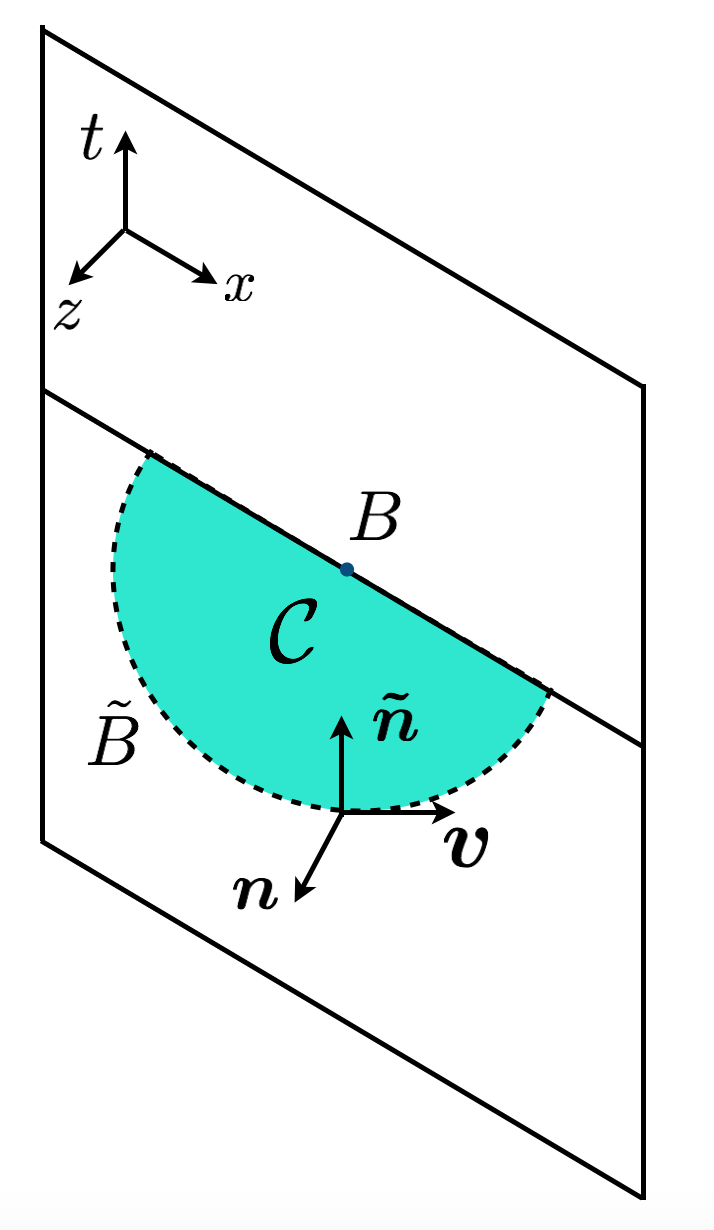
Figure 1: The geometric picture of HEE in TMG. $B$: the boundary interval, $\tilde{B}$: the geodesic homologous to $B$, $\mathcal{C}$: the surface enclosed by $B$ and $\tilde{B}$, $(\bm{v},\bm{n},\bm{\tilde{n}})$: the normal frame along the geodesic. The plane is the boundary of AdS and CFT lives there.

If the bulk spacetime is locally AdS₃, the curve $\gamma$ after doing extremization is actually the geodesic. So the entanglement entropy of the boundary interval $B$ is given by the sum of length of the geodesic and twist of the normal frame along the geodesic:

$$S_{\text{HEE}} = \frac{\text{\sf Length}}{4G_{N}}+\frac{\text{\sf Twist}}{4G_{N}\mu}$$ (12)

$$= \frac{1}{4G_{N}}\int_{\tilde{B}}ds\sqrt{g_{\mu\nu}\dot{X}_{\mu}\dot{X}_{\nu}}+\frac{1}{4G_{N}\mu}\int_{\tilde{B}}ds\;g_{\mu\nu}\tilde{n}^{\mu}v^{\rho}\nabla_{\rho}n^{\nu}~{}.$$ (13)

As applications, we consider the EE in thermal CFTs which are holographically dual to BTZ black holes. The standard metric of BTZ black hole takes the form

$$ds^{2}=-\frac{(\rho^{2}-\rho_{+}^{2})(\rho^{2}-\rho_{-}^{2})}{\rho^{2}}d\tau^{2}+\frac{\rho^{2}}{(\rho^{2}-\rho_{+}^{2})(\rho^{2}-\rho_{-}^{2})}d\rho^{2}+\rho^{2}(d\chi+\frac{\rho_{+}\rho_{-}}{\rho^{2}}d\tau)^{2}~{},$$ (14)

where $\rho_{\pm}$ are the radial position of the outer and inner horizons and they are related to the mass and angular momentum of black holes.

Consider the following interval on the boundary plane $(\tau,\chi)$

$$B:\qquad(\tau=0,\chi=-R_{\chi})\rightarrow(\tau=0,\chi=R_{\chi})~{}.$$ (15)

where we used the right arrow symbol to indicate an interval connecting the two endpoints.

Because of the factorization of left-moving and right-moving modes, the EE of this subregion is contributed by the sum of these two sectors. On the other hand, the EE can be calculated using the proposal we reviewed above. Indeed they agree and the result is Castro et al. (2014)

$$S_{\text{EE}} = S_{L}+S_{R}=\frac{c_{L}}{6}\log\Bigg{(}\frac{\beta_{L}}{\pi\varepsilon_{\chi}}\sinh\Big{(}\frac{2\pi R_{\chi}}{\beta_{L}}\Big{)}\Bigg{)}+\frac{c_{R}}{6}\log\Bigg{(}\frac{\beta_{R}}{\pi\varepsilon_{\chi}}\sinh\Big{(}\frac{2\pi R_{\chi}}{\beta_{R}}\Big{)}\Bigg{)}$$ (16)

$$= S_{\text{RT}}+S_{\text{CS}}=\frac{c_{L}+c_{R}}{12}\log\Bigg{(}\frac{\beta_{L}\beta_{R}}{\pi^{2}\varepsilon_{\chi}^{2}}\sinh\Big{(}\frac{2\pi R_{\chi}}{\beta_{L}}\Big{)}\sinh\Big{(}\frac{2\pi R_{\chi}}{\beta_{R}}\Big{)}\Bigg{)}$$ (18)

$$\qquad\qquad\qquad+\frac{c_{L}-c_{R}}{12}\log\Bigg{(}\frac{\beta_{L}\sinh\Big{(}\frac{2\pi R_{\chi}}{\beta_{L}}\Big{)}}{\beta_{R}\sinh\Big{(}\frac{2\pi R_{\chi}}{\beta_{R}}\Big{)}}\Bigg{)}~{},$$

where the temperature of the left-mover and right-mover in CFT are related to the mass and angular momentum of BTZ black hole. More precisely, they are

$$\beta_{L}=\frac{2\pi}{\rho_{+}-\rho_{-}},\qquad\beta_{R}=\frac{2\pi}{\rho_{+}+\rho_{-}}~{}.$$ (19)

For our convenience, we would like to translate the results above into another coordinate system. The phase space of AdS₃ solutions are given by

$$ds^{2}=\frac{dr^{2}}{4r^{2}}+\Big{(}2r+\frac{U(u)V(v)}{2r}\Big{)}dudv+\Big{(}U(u)du^{2}+V(v)dv^{2}\Big{)}~{}.$$ (20)

With this coordinate, the factorization of left- and right- moving sectors becomes manifest. Wick rotating to the Euclidean signature, the light-cone coordinates $u,v$ become the complex coordinate $z,\bar{z}$.

We are especially interested in the zero mode cases which correspond to constant functions $U,V$ and admit high symmetries

$$ds^{2}=\frac{dr^{2}}{4r^{2}}+\Big{(}2r+\frac{UV}{2r}\Big{)}dudv+\Big{(}Udu^{2}+Vdv^{2}\Big{)}~{}.$$ (21)

They are essentially the BTZ black holes (14). The two coordinate systems are related through

$$\rho=\frac{\sqrt{(r+\rho_{-}^{2})^{2}+2(r-\rho_{-}^{2})\rho_{+}^{2}+\rho_{+}^{4}}}{2\sqrt{r}},\quad\chi=\sqrt{2}(u+v),\quad\tau=\sqrt{2}(u-v)~{},$$ (22)

and

$$U=2(\rho_{+}+\rho_{-})^{2},\qquad V=2(\rho_{+}-\rho_{-})^{2}~{}.$$ (23)

The horizons of the black holes in our coordinates sit at

$$r_{+}=\rho_{+}^{2}-\rho_{-}^{2}=\frac{1}{2}\sqrt{UV},\qquad r_{-}=-\rho_{+}^{2}+\rho_{-}^{2}=-\frac{1}{2}\sqrt{UV}~{}.$$ (24)

We would like to express the results of EE in terms our coordinate systems. The boundary plane $(u,v)$ and $(\tau,\chi)$ are related through a nontrivial rescaling (22). The interval in (15) in our new coordinate system $(\tau,\chi)$ is expressed as

$$B:\qquad(u=-R,v=-R)\rightarrow(u=R,v=R)~{}.$$ (25)

Then it is easy to see

$$2R_{\chi}=l_{\chi}=\sqrt{2}(l_{u}+l_{v})=4\sqrt{2}R~{},\qquad l_{\tau}=\sqrt{2}(l_{u}+l_{v})=0~{},$$ (26)

yielding

$$R_{\chi}=\sqrt{8}R~{}.$$ (27)

With these relations, we can easily translate the results of EE into our new coordinate system

$$S_{\text{EE}}=S_{\text{RT}}+S_{\text{CS}} = \frac{c_{L}+c_{R}}{12}\log\Bigg{(}\frac{8}{\sqrt{UV}\varepsilon_{\chi}^{2}}\sinh\Big{(}2R\sqrt{U}\Big{)}\sinh\Big{(}2R\sqrt{V}\Big{)}\Bigg{)}$$ (28)

$$+ \frac{c_{L}-c_{R}}{12}\log\Bigg{(}\frac{\sqrt{V}\sinh\Big{(}2R\sqrt{U}\Big{)}}{\sqrt{U}\sinh\Big{(}2R\sqrt{U}\Big{)}}\Bigg{)}~{}.$$ (29)

Consider the limit that $U,V$ are small perturbations, then

$$S_{\text{EE}}=\frac{1}{2G}\Big{(}\log\frac{R}{\varepsilon}+\frac{R^{2}}{3}(U+V)\Big{)}+\frac{1}{6G\mu}R^{2}(U-V)+o(U,V)~{},$$ (30)

where $\varepsilon=\varepsilon_{\chi}/\sqrt{32}$ and we used the dictionary of central charges.

As a byproduct of this paper, in the appendix B we will derive the entanglement entropy using other two different approaches: Rindler method and integration in the phase space. The second method applies to arbitrary zero mode background (namely arbitrary temperature CFT) and arbitrary interval (not necessarily on the constant time slice). These results reduce to the known results in the proper limit. The key point is regarding the entanglement entropy, like the black hole entropy, as a Noether charge. This is quite generic and should be applicable to much wider classes, especially to those non-AdS holography.

2.3 Symmetries and modular flow

For later discussions, we also need to understand the symmetries and the modular flow.

Consider the following interval on the boundary of AdS (in Minkowski coordinate $(t,x)$)

$$B:\qquad(0,-R)\rightarrow(0,R)~{},$$ (31)

For every interval, one can associate a Killing vector generating the modular flow. This modular flow generator can be obtained through the Rindler method. Especially for the interval in (31), it is Casini et al. (2011)

$$\xi_{B}=-\frac{2\pi t}{R}(z\partial_{z}+x\partial_{x})+\frac{\pi}{R}(R^{2}-z^{2}-t^{2}-x^{2})\partial_{t}~{}.$$ (32)

Restricting to the boundary of AdS, it reduces to

$$\zeta_{B}=-\frac{2\pi tx}{R}\partial_{x}+\frac{\pi}{R}(R^{2}-t^{2}-x^{2})\partial_{t}~{}.$$ (33)

More generally, one can study the boosted interval. It is convenient to introduce the light-cone coordinates due to the factorization of the left and righer movers

$$ds^{2}=G^{(0)}_{\mu\nu}dx^{\mu}dx^{\nu}=\frac{dz^{2}-dt^{2}+dx^{2}}{z^{2}}=\frac{dr^{2}}{4r^{2}}+2rduduv~{},$$ (34)

The two coordinate systems are related through

$$r=\frac{1}{2z^{2}},\qquad u=x+t,\qquad v=x-t~{}.$$ (35)

The most general subregion of interest is then given by

$$-(\frac{l_{u}}{2},\frac{l_{v}}{2})\rightarrow(\frac{l_{u}}{2},\frac{l_{v}}{2})~{}.$$ (36)

The associated Killing vector can also be obtained through Rindler method. See appendix A for details where we also work out the modular flow in the most general BTZ background. The result is

$$\xi = -\frac{2\pi}{l_{u}}L_{1}+\frac{\pi l_{u}}{2}L_{-1}+\frac{2\pi}{l_{v}}\bar{L}_{1}-\frac{\pi l_{v}}{2}\bar{L}_{-1}$$ (37)

$$= 4\pi r\Big{(}\frac{u}{l_{u}}-\frac{v}{l_{v}}\Big{)}\partial_{r}+\frac{\pi}{2}\Big{(}l_{u}-\frac{2}{rl_{v}}-\frac{4u^{2}}{l_{u}}\Big{)}\partial_{u}-\frac{\pi}{2}\Big{(}l_{v}-\frac{2}{rl_{u}}-\frac{4v^{2}}{l_{v}}\Big{)}\partial_{v}~{}.$$ (38)

On the boundary, it reduces to

$$\zeta=\frac{\pi}{2}\Big{(}l_{u}-\frac{4u^{2}}{l_{u}}\Big{)}\partial_{u}-\frac{\pi}{2}\Big{(}l_{v}-\frac{4v^{2}}{l_{v}}\Big{)}\partial_{v}~{}.$$ (39)

It is easy to see that at the endpoints of the interval $r=\infty,u=\pm\frac{l_{u}}{2},v=\pm\frac{l_{v}}{2}$, the modular flow vanishes $\zeta=\xi=0$. The unboosted interval corresponds to $l_{u}=l_{v}=2R$ and the above general form reduces to the special case.

The RT-HRT minimal surface, more precisely the geodesic here, coincides with the fixed points of the modular flow $\xi=0$:

$$u=l_{u}\sqrt{\frac{1}{4}-\frac{1}{2rl_{u}l_{v}}}~{},\qquad v=l_{v}\sqrt{\frac{1}{4}-\frac{1}{2rl_{u}l_{v}}}~{}.$$ (40)

In the special case of constant time slice $l_{t}=0$,

$$l_{u}=l_{v}=2R:\qquad x^{2}+z^{2}=R^{2}~{}.$$ (41)

2.4 Variation of entanglement entropy

In this subsection, we want to investigate the variation of entanglement entropy around the vacuum state whose dual geometry is the Poincare AdS (34). The variations of the vacuum state correspond to the fluctuations of the bulk metric.

First we consider the Einstein-Hilbert contribution to the variation of EE. Using the RT-HRT proposal for HEE, we should consider the variation of geodesic length in the bulk. Since the geodesic is an extremal curve in the bulk, to leading order, the position of geodesic should not be modified and the only contribution comes from the change of induced metric along the geodesic Lashkari et al. (2014). So to leading order, the variation of EE from Einstein-Hilbert term is

$$\delta S_{\text{RT}}=\delta\frac{1}{4G_{N}}\int_{\tilde{B}}ds=\delta\frac{1}{4G_{N}}\int_{\tilde{B}}d\lambda\sqrt{G_{\mu\nu}\dot{x}^{\mu}\dot{x}^{\nu}}=\frac{1}{8G_{N}}\int_{\tilde{B}}d\lambda\frac{\delta G_{\mu\nu}\dot{x}^{\mu}\dot{x}^{\nu}}{\sqrt{G^{(0)}_{\mu\nu}\dot{x}^{\mu}\dot{x}^{\nu}}}~{},$$ (42)

where $\tilde{B}$ is the geodesic in the unperturbative background.

For the CS term, we begin with a condition in the normal frame $n\cdot\tilde{n}=n^{\nu}\tilde{n}_{\nu}=0$, which immediately implies that

$$\nabla_{\rho}(n^{\nu}\tilde{n}_{\nu})=n^{\nu}\nabla_{\rho}\tilde{n}_{\nu}+\nabla_{\rho}n^{\nu}\tilde{n}_{\nu}=0~{},$$ (43)

This enables us to rewrite

$$S_{\text{CS}}=\frac{1}{4G_{N}\mu}\int_{\tilde{B}}ds\;v^{\rho}\tilde{n}_{\nu}\nabla_{\rho}n^{\nu}=\frac{1}{8G_{N}\mu}\int_{\tilde{B}}ds\;v^{\rho}\Big{(}\tilde{n}_{\nu}\nabla_{\rho}n^{\nu}-n_{\nu}\nabla_{\rho}\tilde{n}^{\nu}\Big{)}~{}.$$ (44)

Now consider the fluctuation of the background metric. As in Einstein-Hilbert case, to leading order, the position of the geodesic is not modified and the only variation of EE in CS term is accounted for by the variation of the induced metric along the geodesic. More precisely we only need to consider the variation of covariant derivatives $\delta\nabla=\delta(\partial+\Gamma)=\delta\Gamma$.

Therefore

$$\delta S_{\text{CS}} = \frac{1}{8G_{N}\mu}\int_{\tilde{B}}ds\;v^{\rho}\Big{(}\tilde{n}_{\nu}\delta\Gamma_{\rho\sigma}^{\nu}n^{\sigma}-n_{\nu}\delta\Gamma_{\rho\sigma}^{\nu}\tilde{n}^{\sigma}\Big{)}$$ (45)

$$= \frac{1}{8G_{N}\mu}\int_{\tilde{B}}ds\;v^{\rho}\delta\Gamma_{\rho\sigma}^{\nu}g_{\mu\nu}\Big{(}\tilde{n}^{\mu}n^{\sigma}-n^{\mu}\tilde{n}^{\sigma}\Big{)}~{}.$$ (46)

Since $\tilde{B}$ is the bifurcate horizon of modular flow generator $\xi_{B}$, we have

$$\text{on }\tilde{B}:\qquad\xi_{B}=0,\qquad\epsilon^{\mu\sigma}\equiv\tilde{n}^{\mu}n^{\sigma}-n^{\mu}\tilde{n}^{\sigma}=\frac{1}{\kappa_{\xi_{B}}}\nabla^{\mu}\xi_{B}^{\sigma}~{},\qquad$$ (47)

where $\epsilon^{\mu\sigma}$ is called binormal and the surface gravity on the Killing horizon is defined as

$$\xi^{\alpha}\nabla_{\alpha}\xi_{\beta}=\kappa\xi_{\beta}~{}.$$ (48)

Thus to leading order, the variation of EE from CS term is

$$\delta S_{\text{CS}} = \frac{1}{8G_{N}\mu}\int_{\tilde{B}}ds\;v^{\rho}\delta\Gamma_{\rho\sigma}^{\nu}g_{\mu\nu}\epsilon^{\mu\sigma}=\frac{1}{8\pi G_{N}\mu\kappa_{\xi_{B}}}\int_{\tilde{B}}ds\;v^{\rho}\delta\Gamma_{\rho\sigma}^{\nu}\nabla_{\nu}\xi_{B}^{\sigma}$$ (49)

$$= \frac{1}{8\pi G_{N}\mu\kappa_{\xi_{B}}}\int_{\tilde{B}}dx^{\rho}\delta\Gamma_{\rho\sigma}^{\nu}\partial_{\nu}\xi_{B}^{\sigma}~{}.$$ (50)

For the modular flow generator in (32) and (38), the surface gravity is $\kappa=2\pi$. So

$$\delta S_{\text{CS}} = \frac{1}{8G_{N}\mu}\int_{\tilde{B}}ds\;v^{\rho}\delta\Gamma_{\rho\sigma}^{\nu}g_{\mu\nu}\epsilon^{\mu\sigma}=\frac{1}{16\pi G_{N}\mu}\int_{\tilde{B}}ds\;v^{\rho}\delta\Gamma_{\rho\sigma}^{\nu}\partial_{\nu}\xi^{\sigma}~{}.$$ (51)

This expression coincides with the infinitesimal version of black hole entropy from CS term Tachikawa (2007). Note that this is a covariant expression. Although the Christoffel symbol is not a tensor, its variation indeed is a tensor. This expression can also be derived using the Rinlder method which maps the entanglement entropy to thermal entropy and geodesic (a bifurcate horzion of modular flow) to the black hole horizon. The covariant properties of the expression guarantee that the form is the same before and after Rindler transformation.

As a check of our proposal, we can consider the zero mode fluctuations around the vacuum. Then the fluctuated metric is given by (21) with $U,V$ being small. Using our formulae above, we easily find that

$$\delta S_{\text{CS}} = \frac{1}{4G\mu}\frac{1}{4\pi}\int_{\tilde{B}}ds\;v^{\rho}\delta\Gamma^{\nu}_{\sigma\rho}\partial_{\nu}\xi^{\sigma}=\frac{1}{6G\mu}R^{2}(U-V)~{},$$ (52)

$$\delta S_{\text{RT}} = \frac{1}{4G}\int_{\tilde{B}}dr\;\delta\sqrt{\frac{1}{4r^{2}}+\Big{(}2r+\frac{UV}{2r}+U+V\Big{)}(\frac{du}{dr})^{2}}=\frac{R^{2}}{6G}(U+V)~{}.$$ (53)

We see that our perturbative calculations here agree with the exact result (30). In the following sections, we will consider generic fluctuations which are not necessarily constant modes and explore the physical implications.

3 Holographic dictionary of stress tensor from entanglement

As an important ingredient in holography, the holography dictionary establishes a map between the boundary field theory and bulk gravity. The standard approach to build the holographic dictionary is using holographic renormalization. Especially, the energy-momentum tensor of boundary CFT is given by the metric fluctuation in the bulk AdS gravity. In the presence of the CS term/gravitational anomalies, the dictionary becomes more complicated and the complete derivation was done in Skenderis et al. (2009).

In Faulkner et al. (2014), using holographic entanglement the authors found an alternative simple way to derive the dictionary of energy-momentum tenor in the Einstein gravity and higher derivative gravity. In this section, we will generalize their method and derive the dictionary in the presence of CS term/gravitational anomalies. For simplicity, we focus on 3D gravity. But the method here could be easily generalized to higher dimensions.

3.1 Holographic dictionary from the first law of entanglement

Consider the Fefferman-Graham expansion of asymptotic AdS₃ around the vacuum state

$$ds^{2}=\frac{dz^{2}-dt^{2}+dx^{2}}{z^{2}}+h_{ij}(z,t,x)dx^{i}dx^{j}~{}.$$ (54)

In this paper, we restrict ourselves to the asymptotic locally AdS case, so $h_{ij}(z,t,x)\rightarrow o(\frac{1}{z^{2}})$ near the boundary. The dictionary with more general boundary conditions is considered in Skenderis et al. (2009), but we are not going to explore it here partly because the entanglement entropy beyond AdS is not well understood yet.

We consider the following interval

$$B:\qquad(t=0,x=-R)\rightarrow(t=0,x=R)~{}.$$ (55)

The key point in the derivation is the first law of entanglement

$$\delta\langle H_{\text{mod }}\rangle=\delta S_{\text{HEE}}~{},$$ (56)

which relates the variation of vacuum expectation value of modular Hamiltonian and the variation of holographic entanglement entropy. Let us first consider the variation of holographic entanglement entropy about the vacuum state. It has two contribution. The Einstein-Hilbert contribution can be considered using the RT-HRT proposal, given by the variation of geodesic length. To leading order, as we discussed in the last section, it is

$$\delta S_{\text{RT}}=\delta\frac{1}{4G_{N}}\int_{\tilde{B}}ds=\frac{1}{8G_{N}}\int_{\tilde{B}}d\lambda\frac{\delta G_{\mu\nu}\dot{x}^{\mu}\dot{x}^{\nu}}{\sqrt{G^{(0)}_{\mu\nu}\dot{x}^{\mu}\dot{x}^{\nu}}}~{},$$ (57)

where $\tilde{B}$ is the geodesic. While for the CS term, as we derived in the last section, the contribution is given by

$$\delta S_{\text{CS}}=\frac{1}{4G\mu}\frac{1}{4\pi}\int_{\tilde{B}}ds\;v^{\rho}\delta\Gamma^{\nu}_{\sigma\rho}\partial_{\nu}\xi^{\sigma}~{}.$$ (58)

For the metric fluctuation given in (54), the explicit results are

$$\delta S_{\text{RT}} = \frac{1}{4G}\int_{-R}^{R}dx\frac{R^{2}-x^{2}}{2R}h_{xx}(z,0,x)~{},\qquad z=\sqrt{R^{2}-x^{2}}~{},$$ (59)

$$\delta S_{\text{CS}} = \frac{1}{4G\mu}\int_{-R}^{R}dx\frac{R^{2}-x^{2}}{2R}\Bigg{(}h_{tx}(z,0,x)+z\partial_{z}h_{tx}(z,0,x)+x\Big{(}\partial_{x}h_{tx}(z,0,x)-\partial_{t}h_{xx}(z,t,x)|_{t=0}\Big{)}\Bigg{)}~{}.\qquad$$ (60)

And their sum is

$$\delta S = \frac{1}{4G}\int_{-R}^{R}dx\frac{R^{2}-x^{2}}{2R}\Bigg{(}h_{xx}(z,0,x)+\frac{1}{\mu}h_{tx}(z,0,x)$$ (61)

$$\qquad\qquad\qquad+\frac{1}{\mu}z\partial_{z}h_{tx}(z,0,x)+\frac{1}{\mu}x\Big{(}\partial_{x}h_{tx}(z,0,x)-\partial_{t}h_{xx}(z,t,x)|_{t=0}\Big{)}\Bigg{)}~{}.$$

We want to consider the limit $R\rightarrow 0$. In this case, $x,z\sim R\rightarrow 0$ and

$$\delta S \xrightarrow{R\rightarrow 0} \frac{1}{4G}\int_{-R}^{R}dx\frac{R^{2}-x^{2}}{2R}\Bigg{(}h_{xx}(z,0,x)+\frac{1}{\mu}h_{tx}(z,0,x)$$ (62)

$$\qquad\qquad\qquad+\frac{1}{\mu}z\partial_{z}h_{tx}(z,0,x)+\frac{1}{\mu}x\Big{(}\partial_{x}h_{tx}(z,0,x)-\partial_{t}h_{xx}(z,t,x)|_{t=0}\Big{)}\Bigg{)}\Bigg{|}_{z=x=t=0}$$

$$= \frac{1}{4G}\int_{-R}^{R}dx\frac{R^{2}-x^{2}}{2R}\times\Bigg{(}h_{xx}(0,0,0)+\frac{1}{\mu}h_{tx}(0,0,0)+\frac{1}{\mu}z\partial_{z}h_{tx}(z,0,0)|_{z=0}\Big{)}$$

$$= \frac{R^{2}}{6G}\Bigg{(}h_{xx}(0,0,0)+\frac{1}{\mu}h_{tx}(0,0,0)+\frac{1}{\mu}\frac{\partial}{\partial\log z}h_{tx}(z,0,0)|_{z=0}\Bigg{)}~{}.$$

At first glance, the last term in the bracket should be discarded because of the divergence in $\log z$ near the boundary. However, we don’t know the $z$-dependence of the function. In order to have a finite answer, there could be a $\log z$ linear dependence in $h_{tx}$ to regulate the divergence in $z$. So we can have the following general ansatz

$$h_{ij}(z,x^{k})=2\log z\,B_{ij}(x^{k})+H_{ij}(x^{k})+...~{},$$ (63)

where the ellipsis denotes the higher order terms in $z$ which have no contribution in $\delta S$.

Plugging the ansatz back, we get

$$\delta S\xrightarrow{R\rightarrow 0}\frac{R^{2}}{6G}\Big{(}H_{xx}+\frac{1}{\mu}H_{tx}+2\frac{1}{\mu}B_{tx}+2\frac{1}{\mu}\log z(B_{xx}+\frac{1}{\mu}B_{tx})\Big{)}\Big{|}_{z=t=x=0}~{}.$$ (64)

In order to have a finite answer on the boundary, the coefficient of $\log z$ should vanish

$$B_{xx}=-\frac{1}{\mu}B_{tx}~{}.$$ (65)

In this case, we have

$$\delta S\xrightarrow{R\rightarrow 0}\frac{R^{2}}{6G}\Big{(}H_{xx}(x=t=0)+\frac{1}{\mu}H_{tx}(x=t=0)-2B_{xx}(x=t=0)\Big{)}~{}.$$ (66)

On the other hand, the modular Hamiltonian in CFT is given by

$$H=\int_{B}\zeta_{B}^{\mu}T_{\mu\nu}\epsilon^{\nu}=2\pi\int_{-R}^{R}dx\frac{(R^{2}-x^{2})}{2R}T_{tt}~{}.$$ (67)

And its infinitesimal variation is

$$\delta\langle H\rangle\xrightarrow{R\rightarrow 0}2\pi\int_{-R}^{R}dx\frac{(R^{2}-x^{2})T_{tt}}{2R}=\frac{4\pi R^{2}}{3}\delta\langle T_{tt}(x=t=0)\rangle~{}.$$ (68)

Using the first law of entanglement $\delta S=\delta\langle H\rangle$, we thus find

$$\langle T_{tt}\rangle=\frac{1}{8\pi G_{N}}\Big{(}H_{xx}+\frac{1}{\mu}H_{tx}-2B_{xx}\Big{)}~{}.$$ (69)

We would like to generalize it to arbitrary Lorentz frame. This can be done by considering the boosted interval and repeat all the discussions again. Another way is to use the Lorentz invariance and covariantize the above formula. Note that $H_{xx}=H^{x}{}_{x}=H_{tt}-\eta_{tt}H^{k}{}_{k}$ and $H_{tx}=-\epsilon_{t}{}^{x}H_{xt}=-\epsilon_{t}{}^{k}H_{kt}$ . So

$$\langle T_{ij}\rangle=\frac{1}{8\pi G_{N}}\Big{(}H_{ij}-\eta_{ij}H^{k}{}_{k}-2B_{ij}+2\eta_{ij}B^{k}{}_{k}-\frac{1}{2\mu}\epsilon_{i}{}^{k}H_{kj}-\frac{1}{2\mu}\epsilon_{j}{}^{k}H_{ki}\Big{)}~{}.$$ (70)

The tracelessness of the energy-momentum tensor in CFT $T^{i}{}_{i}=0$ implies the traceless of metric fluctuation

$$H^{k}{}_{k}=B^{k}{}_{k}=0~{}.$$ (71)

This enables us to rewrite

$$\langle T_{ij}\rangle=\frac{1}{8\pi G_{N}}\Bigg{(}H_{ij}-2B_{ij}-\frac{1}{2\mu}\Big{(}\epsilon_{i}{}^{k}H_{kj}+i\leftrightarrow j\Big{)}\Bigg{)}~{}.$$ (72)

However, this is not the end of story.

3.2 Further constraints from Lorentz invariance

From (65) and (71) we have

$$B_{xx}=B_{tt}=-\frac{1}{\mu}B_{xt}=-\frac{1}{\mu}B_{tx}~{}.$$ (73)

This is actually inconsistent with the Lorentz invariance unless $\mu=\pm 1$. To see this, define the map:

$$\widetilde{}:S_{ij}\mapsto\widetilde{S}_{ik}=\epsilon_{i}{}^{k}S_{kj}~{}.$$ (74)

Especially this is a linear map, implying

$$\widetilde{B}_{xx}=-B_{tx}=\mu B_{xx}~{}.$$ (75)

and furthermore

$$\widetilde{\widetilde{B}}_{xx}=\mu\widetilde{B}_{xx}=\mu^{2}B_{xx}~{}.$$ (76)

On the other, this map is an involution $\;\widetilde{}\;{}^{2}=1$, implying that $\widetilde{\widetilde{B}}_{xx}=B_{xx}$. So these two are inconsistent unless $\mu=\pm 1$. These two values are equivalent up to an orientation. In this paper, without loss of generality, as usual we just consider $\mu=1$. So in general, if $\mu\neq 1$, the logarithmic mode in the asymptotic expansion should vanish $B_{ij}=0$. The logarithmic mode at the chiral point $\mu=1$ is exactly the one discovered in Grumiller and Johansson (2008); Skenderis et al. (2009).

In this case, the (73) can be compactly written as

$$\epsilon_{i}{}^{k}B_{kj}=B_{ij}~{}.$$ (77)

The conservation of the stress tensor in CFT $\partial^{i}T_{ij}=0$ implies that

$$\partial^{i}B_{ij}=0,\qquad(\delta_{i}^{k}-\frac{1}{\mu}\epsilon_{i}{}^{k})\partial^{j}H_{jk}=0~{}.$$ (79)

We can expand the first conservation explicitly

$$0 = \partial^{x}B_{xx}+\partial^{t}B_{tx}=\partial^{x}B_{xx}-\mu\partial^{t}B_{xx}~{},$$ (80)

$$0 = \partial^{x}B_{xt}+\partial^{t}B_{tt}=-\mu\partial^{x}B_{xx}+\partial^{t}B_{xx}=-{\mu}\partial^{x}B_{xx}+\frac{1}{\mu}\partial^{x}B_{xx}~{}.$$ (81)

So these equations are not consistent unless $\mu=\pm 1$. (This argument is defective since it allows another possibility $\partial^{x}B_{xx}=0$ for general $\mu$).

The second equation in (79) can be multiplied by $\epsilon_{l}{}^{i}$ which yields

$$(\epsilon_{l}{}^{i}\delta_{i}^{k}-\frac{1}{\mu}\epsilon_{l}{}^{i}\epsilon_{i}{}^{k})\partial^{j}H_{jk}=\epsilon_{l}{}^{i}\partial^{j}H_{ji}-\frac{1}{\mu}\delta_{i}{}^{k}\partial^{j}H_{jk}=(\mu-\frac{1}{\mu})\partial^{j}H_{jl}=0~{},$$ (82)

where we use (79) repeatedly as well as the property of $\epsilon$.

So, we have

$$\mu=\pm 1:\qquad(\delta_{i}^{k}\mp\epsilon_{i}{}^{k})\partial^{j}H_{jk}=0~{},$$ (83)

or

$$\mu\neq 1:\qquad\partial^{j}H_{jk}=0~{}.$$ (84)

To summarize, based on the first law of entanglement, Lorentz invariance and requiring a finite energy-momentum tensor, we find that

• $\mu=1$: the asymptotic expansion is given by

  $$h_{ij}(z,x^{k})=2\log zB_{ij}(x^{k})+H_{ij}(x^{k})+...$$ (85)

  where $B$ should satisfy the condition

  $$\epsilon_{i}{}^{k}B_{kj}=B_{ij}~{}.$$ (86)

  This is exactly the logarithmic mode for TMG at the chiral point, discovered in Grumiller and Johansson (2008); Skenderis et al. (2009). The holographic dictionary between stress tensor and asymptotic metric is given by

  $$\langle T_{ij}\rangle=\frac{1}{8\pi G_{N}}\Bigg{(}H_{ij}-2B_{ij}-\frac{1}{2}\Big{(}\epsilon_{i}{}^{k}H_{kj}+i\leftrightarrow j\Big{)}\Bigg{)}~{}.$$ (87)

  The conservation of stress tensor enforces

  $$\partial^{i}B_{ij}=0,\qquad(\delta_{i}^{k}-\epsilon_{i}{}^{k})\partial^{j}H_{jk}=0~{}.$$ (88)

  which arises from the EoM of TMG as shown in Skenderis et al. (2009).

• $\mu\neq 1$: the asymptotic expansion is given by

  $$h_{ij}(z,x^{k})=H_{ij}(x^{k})+...$$ (89)

  The holographic dictionary is given by

  $$\langle T_{ij}\rangle=\frac{1}{8\pi G_{N}}\Bigg{(}H_{ij}-\frac{1}{2\mu}\Big{(}\epsilon_{i}{}^{k}H_{kj}+i\leftrightarrow j\Big{)}\Bigg{)}~{}.$$ (90)

  The conservation of stress tensor enforces

  $$\partial^{j}H_{jk}=0~{}.$$ (91)

4 Wald-Tachikawa covariant phase space formalism

In this section, we review the covariant phase space formalism Wald (1993); Iyer and Wald (1994); Tachikawa (2007) which is useful for later discussions on equation of motion and relative entropy.

In the presence of CS term, the theory is not diffeormorphic invariant anymore. Acting with a vector field, besides the normal Lie derivative action, there are also anomalous contributions on the boundary. More specifically, $\delta_{\xi}$ and $\mathcal{L}_{\xi}$ are not the same anymore. To account for the difference, we need to add the anomalous contribution by hand.

4.1 General formalism

We consider the bulk gravity is $(d+1)$-dimensional. The volume form is given by

$${\bm{\epsilon}}=\frac{1}{(d+1)!}\epsilon_{\mu_{1}..\mu_{d+1}}dx^{\mu_{1}}\wedge\cdots\wedge dx^{\mu_{d+1}}~{}.$$ (92)

We also define the following tensors

$${\bm{\epsilon}_{\mu}}=\frac{1}{d!}\epsilon_{\mu\mu_{2}..\mu_{d+1}}dx^{\mu_{2}}\wedge\cdots\wedge dx^{\mu_{d+1}},\qquad{\bm{\epsilon}_{\mu\nu}}=\frac{1}{(d-1)!}\epsilon_{\mu\nu\mu_{3}..\mu_{d+1}}dx^{\mu_{3}}\wedge\cdots\wedge dx^{\mu_{d+1}},\quad\cdots~{}.$$ (93)

The action is given by Lagrangian density integrated over spacetime

$$S=\int\mathcal{L}\bm{\epsilon}=\int\bm{L}~{}.$$ (94)

Its variation gives rise to

$$\delta\bm{L}=\bm{E}_{\phi}\delta\phi+d\bm{\Theta}[\delta\phi]~{},$$ (95)

where $\phi$ collectively denotes all the fields including the metric and $\bm{E}_{\phi}$ is the equation of motion.

In the presence of the CS term, the variation under a diffeomorphism generated by an arbitrary vector field $\xi$ acquires extra contributions, in addition to the Lie derivative action:

$$\delta_{\xi}\bm{L} = \mathcal{L}_{\xi}\bm{L}+d\bm{\Xi}_{\xi}~{},$$ (96)

$$\delta_{\xi}\bm{\Theta} = \mathcal{L}_{\xi}\bm{\Theta}+d\bm{\Pi}_{\xi}~{}.$$ (97)

One can show that the two anomalous terms are related

$$d\bm{\Pi}_{\xi}=\delta d\bm{\Xi}_{\xi}~{},$$ (98)

which implies that

$$\bm{\Pi}_{\xi}-\delta\bm{\Xi}_{\xi}=d\bm{\Sigma}_{\xi}~{}.$$ (99)

We can define the sympletic form

$$\bm{\omega}[\delta_{1}\phi,\delta_{2}\phi]=\delta_{1}\bm{\Theta}[\delta_{2}\phi]-\delta_{2}\bm{\Theta}[\delta_{1}\phi]~{},$$ (100)

and Noether current

$$\bm{J}_{\xi}=\bm{\Theta}[\delta_{\xi}\phi]-\xi\cdot\bm{L}-\bm{\Xi}_{\xi}~{}.$$ (102)

It is easy to check that the Noether current is conserved on-shell

$$d\bm{J}_{\xi}=d\bm{\Theta}-\mathcal{L}_{\xi}\bm{L}-d\bm{\Xi}=-\bm{E}_{\phi}\delta_{\xi}\phi\simeq 0~{}.$$ (103)

In the above derivation we used the Cartan identity

$$\mathcal{L}_{\xi}=d\iota_{\xi}+\iota_{\xi}d~{}.$$ (104)

The conservation of Noether current is expected considering the generalized diffeomorphism invariance. And we can even further define the Noether charge associated to it

$$d\bm{Q}_{\xi}=\bm{J}_{\xi}~{}.$$ (105)

We can also calculate the variation of the Noether current

$$\delta\bm{J}_{\xi}=\bm{\omega}[\delta\phi,\delta_{\xi}\phi]+\delta_{\xi}\bm{\Theta}[\delta\phi]-\xi\cdot(d\bm{\Theta}+\bm{E}_{\phi}\delta\phi)-\delta\bm{\Xi}_{\xi}=\bm{\omega}[\delta\phi,\delta_{\xi}\phi]+d(\bm{\Sigma}_{\xi}+\xi\cdot\bm{\Theta})~{},$$ (106)

where we used the relation (99).

To proceed we need to find a quantity $\bm{C}_{\xi}$ such that

$$\delta\bm{C}_{\xi}=\xi\cdot\bm{\Theta}+\bm{\Sigma}_{\xi}~{},$$ (107)

and define

$$\widetilde{\bm{Q}}_{\xi}=\bm{Q}_{\xi}-\bm{C}_{\xi}~{}.$$ (108)

Then we can prove that

$$\delta d\widetilde{\bm{Q}}_{\xi}=\delta\bm{J}_{\xi}-(\xi\cdot\bm{\Theta}+\bm{\Sigma}_{\xi})=\bm{\omega}~{}.$$ (109)

This means that $\widetilde{\bm{Q}}_{\xi}$ is the Hamiltonian (density) generating the diffeomorphism under $\xi$.

More precisely, we can define the following quantity which generates the diffeomorphism

$$\delta H_{\xi}=\int_{\mathcal{C}}\bm{\omega}[\delta\phi,\delta_{\xi}\phi]=\int_{\mathcal{C}}\Big{(}\delta\bm{J}_{\xi}-d(\bm{\mathcal{C}}_{\xi}+\xi\cdot\bm{\Theta})\Big{)}=\int_{\partial{\mathcal{C}}}\Big{(}\delta\bm{Q}_{\xi}-\bm{\mathcal{C}}_{\xi}-\xi\cdot\bm{\Theta}\Big{)}~{}.$$ (110)

We will always use $\bm{\chi}$ to denote the integrand, namely $\delta H_{\xi}=\int_{\partial{\mathcal{C}}}d\bm{\chi}$.

If we can find $\bm{N}_{\xi}[\phi],\bm{K}[\phi]$ such that

$$\delta\bm{N}_{\xi}=\bm{\Sigma}_{\xi},\qquad\delta(\xi\cdot\bm{K})=\xi\cdot\bm{\Theta}[\delta\phi]\quad on\quad\partial\mathcal{C}~{},$$ (112)

then we can integrate in the phase space and define

$$H_{\xi}=\int_{\mathcal{C}}\bm{J}_{\xi}-\int_{\partial{\mathcal{C}}}\Big{(}\bm{N}_{\xi}+\xi\cdot\bm{K}\Big{)}=\int_{\partial\mathcal{C}}\Big{(}\bm{Q}_{\xi}-\bm{N}_{\xi}-\xi\cdot\bm{K}\Big{)}=\int_{\partial\mathcal{C}}\widetilde{\bm{Q}}_{\xi}~{},$$ (113)

where we used the relation

$$\xi\cdot\bm{K}=\bm{C}_{\xi}-\bm{N}_{\xi}~{},$$ (114)

which can be derived from (107).

It is worth mentioning that although various quantities suffer ambiguities in their definition, the integrated charge is well-defined and physical. And if the CS term is absent, $\bm{\Xi},\bm{\Pi},\bm{\Sigma},\bm{C},\bm{\tilde{Q}},\bm{N}$ are not needed, as in the pure Einstein gravity case.

4.2 Explicit expressions for TMG

In this paper, we consider the TMG which consists of Einstein-Hilbert term (including cosmological constant term) and CS term. The linearity of the charge enables us to consider them separately. For the pure CS term, we can make a choice such that $\bm{\Sigma}_{\xi}=0$, hence also $\bm{N}_{\xi}=0$ Tachikawa (2007). Some explicit expressions for Einstein-Hilbert term and CS term are given as follows Faulkner et al. (2014); Cheng et al. (2016).

The integrands in the Hamiltonian generating infinitesimal diffeomorphism are

$${\bm{\chi}}_{\xi}^{EH}[\delta g] = \delta\bm{Q}^{EH}_{\xi}-\xi\cdot\bm{\Theta}^{EH}$$ (115)

$$= \frac{1}{16\pi G_{N}}\bm{\epsilon}_{\mu\nu}\Big{(}\xi^{\mu}\nabla_{\sigma}\delta g^{\nu\sigma}-\xi^{\mu}\nabla^{\nu}\delta g_{\sigma}^{\;\sigma}+\xi_{\sigma}\nabla^{\nu}\delta g^{\mu\sigma}+\frac{1}{2}\delta g_{\sigma}^{\;\sigma}\nabla^{\nu}\xi^{\mu}-\delta g^{\sigma\nu}\nabla_{\sigma}\xi^{\mu}\Big{)}~{},\qquad\qquad$$ (116)

$${\bm{\chi}}_{\xi}^{\text{CS}}[\delta g] = \delta\tilde{\bm{Q}}_{\xi}^{\text{CS}}=\frac{1}{32\pi G_{N}\mu}\Bigg{[}2\delta\Gamma^{\nu}_{\beta\mu}\Big{(}\partial_{\nu}\xi^{\mu}+\xi^{\rho}\Gamma^{\mu}_{\nu\rho}\Big{)}+\xi^{\alpha}\Big{(}\delta g_{\alpha\beta}R+g_{\alpha\beta}\delta R-4\delta R_{\alpha\beta}\Big{)}$$ (117)

$$\qquad\qquad\qquad\qquad\qquad\qquad\qquad\qquad-2g^{\mu\nu}\xi^{\alpha}\Big{(}\delta g_{\beta\mu}R_{\alpha\nu}-\delta g_{\alpha\mu}R_{\beta\nu}\Big{)}\Bigg{]}dx^{\beta}~{}.$$

The Noether charges are

$$\bm{Q}_{\xi}^{EH} = -\frac{1}{16\pi G_{N}}\nabla^{\mu}\xi^{\nu}\bm{\epsilon}_{\mu\nu}~{},$$ (118)

$$\bm{Q}_{\xi}^{\text{CS}} = \frac{1}{32\pi G_{N}\mu}\Bigg{[}\Gamma^{\nu}_{\beta\mu}\Big{(}2\partial_{\nu}\xi^{\mu}+\xi^{\rho}\Gamma^{\mu}_{\nu\rho}\Big{)}+\xi^{\alpha}\Big{(}\delta g_{\alpha\beta}R+g_{\alpha\beta}\delta R-4\delta R_{\alpha\beta}\Big{)}\Bigg{]}dx^{\beta}~{}.$$ (119)

The Noether currents are

$${\bm{J}}_{\xi}^{\text{EH}} = d{\bf Q}_{\xi}^{\text{EH}}+2\xi^{\mu}E^{g}_{\mu\nu}{\bm{\epsilon}}^{\nu},\qquad E^{g}_{\mu\nu}=\frac{1}{16\pi G_{N}}(R_{\mu\nu}-\frac{1}{2}g_{\mu\nu}R+\Lambda g_{\mu\nu})~{},$$ (120)

$${\bm{J}}_{\xi}^{\text{CS}} = d{\bf Q}_{\xi}^{\text{CS}}+\frac{1}{32\pi G_{N}\mu}2\xi^{\mu}C_{\mu\nu}{\bm{\epsilon}}^{\nu}~{}.$$ (121)

Note that these expressions hold off-shell and have the form $\bm{J}=d\bm{Q}+\xi^{a}\bm{C}_{a}$ with $\bm{C}_{a}$ the constraints (equation of motion).

5 Linearized equation of motion in TMG from entanglement

In the previous section, we used the first law of entanglement to derive the holographic dictionary of stress tensor by considering the $R\rightarrow 0$ limit of the interval. It is reasonable to expect that the finite $R$ cases will give rise to more higher order constraints. In Lashkari et al. (2014), the authors implemented this method for Einstein gravity and showed that all order constraints are equivalent to the linearized Einstein equation. A more elegant approach based on the Wald formalism was used to prove the linearized equation of motion from HEE in higher derivative gravities. In this section, we will adopt a similar strategy and derive the linearized equation of motion in TMG from HEE. The tool which bridges two sides is the Wald-Tachikawa formalism which is a generalization of Wald formalism and takes into account the Cherns-Simons contribution, as we have reviewed in the last section.

5.1 From non-local constraints to integral constraints

Before discussing the equation of motion, we first prove two important equations:

$$\delta E_{B}^{grav} \equiv \int_{B}\bm{\chi}=\delta\langle H\rangle~{},$$ (122)

$$\delta S_{B}^{grav} \equiv \int_{\tilde{B}}\bm{\chi}=\delta S_{\text{HEE}}~{}.$$ (123)

We specialise to case that the entanglement interval $B:(t=0,x=-R)\rightarrow(t=0,x=R)$ sits on a constant time slice and centers at the origin. We can then use the translation and boost symmetry of the boundary plane to consider all other intervals. A direct way to consider the boosted interval is also straightforward by using the modular flow generator (38) of the boosted interval.

Let us first consider the story on the asymptotic boundary $B$. Substituting the metric fluctuations (54) into (116) and (117), we get

$$\int_{B}\bm{\chi}^{\text{EH}}=\frac{1}{16\pi G_{N}}\frac{2\pi}{R}\int_{-R}^{R}\Big{[}(R^{2}-x^{2})h_{xx}(z,0,x)+\frac{z}{2}(R^{2}-x^{2}-z^{2})\partial_{z}h_{xx}(z,0,x)\Big{]}\Big{|}_{z=0}dx~{},\qquad$$ (124)

and

$$\int_{B}\bm{\chi}^{\text{CS}} = \frac{1}{16\pi G_{N}}\frac{4\pi}{R}\int_{-R}^{R}\Big{[}(R^{2}-x^{2})h_{tx}(z,0,x)+xz^{2}(\partial_{x}h_{tx}(z,0,x)-\partial_{t}h_{xx}(z,t,x)|_{t=0})$$ (125)

$$\qquad+z(2R^{2}-2x^{2}-z^{2})\partial_{z}h_{tx}(z,0,x)+\frac{1}{2}z^{2}(R^{2}-x^{2}-z^{2})\partial_{z}^{2}h_{tx}(z,0,x)\Big{]}\Big{|}_{z=0}dx~{}.\qquad\qquad$$

Since we are now interested in the asymptotic boundary, we can further specialise to the near boundary expansion (63) of the metric fluctuations. Substituting it into the above two expressions, we get their sum

$$\delta E_{B}^{grav}\equiv\int_{B}\bm{\chi} = \frac{1}{8G_{N}}\int_{-R}^{R}\frac{R^{2}-x^{2}}{R}\Bigg{[}H_{xx}(0,x)+B_{xx}(0,x)+\frac{H_{tx}(0,x)+3B_{tx}(0,x)}{\mu}\qquad\qquad$$ (126)

$$\qquad\qquad\qquad\qquad\qquad+2\log z\Big{(}B_{xx}(0,x)+\frac{1}{\mu}B_{tx}(0,x)\Big{)}\Bigg{]}dx~{}.$$

The coefficient of $\log z$ should be zero otherwise the quantity is divergent on the boundary. The resulting requirement is exactly the same as the one we derived in (65). As argued before, in the presence of the log mode $B_{ij}$, the Lorentz invariance is only preserved at the chiral point $\mu=1$. Thus,

$$\delta E_{B}^{grav}\equiv\int_{B}\bm{\chi} = \frac{1}{8G_{N}}\int_{-R}^{R}\frac{R^{2}-x^{2}}{R}\Bigg{[}H_{xx}(0,x)+\frac{1}{\mu}H_{tx}(0,x)+2B_{tx}(0,x)\delta_{\mu,1}\Bigg{]}dx~{}.$$ (127)

It is easy to see that this equations is exactly the same as the expression of modular Hamiltonian (67) when the holographic dictionaries (87), (90) are used. Therefore,

$$\delta E_{B}^{grav}=\delta\langle H\rangle~{}.$$ (128)

More generally, using Lorentz invariance or considering arbitrary boosted intervals, we have the covariant expression of the integrand

$$\bm{\chi}|_{\partial M}=d\Sigma^{\mu}T_{\mu\nu}^{grav}\zeta^{\nu}~{}.$$ (129)

Especially, the conservation and traceless of the CFT stress tensor implies that

$$d\bm{\chi}|_{\partial M}=0~{}.$$ (130)

This property ensures that on the boundary we can actually consider arbitrary path which connects the endpoints of $B$ and $\delta E_{B}^{grav}$ is independent of the choice of the path. This is consistent with the requirement that the entanglement entropy should be a function of the causal development of the interval.

Now we switch to the story on the geodesic $\tilde{B}$. This is a bifurcate horizon such that $\xi|_{\tilde{B}}=0$ and $\nabla^{a}\xi^{b}|_{\tilde{B}}=2\pi\epsilon^{ab}$.

For the Einstein part, using (118), we have

$$\int_{\tilde{B}}\bm{Q}_{\xi}^{\text{EH}}=-\frac{1}{16\pi G_{N}}\int_{\tilde{B}}\nabla^{a}\xi^{b}\bm{\epsilon}_{ab}=\frac{1}{4G}{\sf Length}(\tilde{B})~{},$$ (131)

thus

$$\int_{\tilde{B}}{\bm{\chi}}_{\xi}^{\text{EH}}=\int_{\tilde{B}}\delta\bm{Q}_{\xi}^{\text{EH}}=\frac{1}{4G}\delta{\sf Length}(\tilde{B})=\delta S_{\text{RT}}~{}.$$ (132)

While for the CS part, the infinitesimal charge (117) simplifies a lot on the bifurcate horizon where the modular flow vanishes

$${\bm{\chi}}_{\xi}^{\text{CS}}|_{\tilde{B}}=\frac{1}{16\pi G_{N}\mu}\delta\Gamma^{\nu}_{\beta\mu}\partial_{\nu}\xi^{\mu}dx^{\beta}~{},$$ (133)

therefore

$$\int_{\tilde{B}}{\bm{\chi}}_{\xi}^{\text{CS}}|_{\tilde{B}}=\frac{1}{16\pi G_{N}\mu}\int_{\tilde{B}}dx^{\beta}\delta\Gamma^{\nu}_{\beta\mu}\partial_{\nu}\xi^{\mu}=\delta S_{\text{CS}}~{},$$ (134)

where for the last equality, we observe that the expression in the middle coincides with (51).

So we conclude that

$$\delta S_{B}^{grav}\equiv\int_{\tilde{B}}\bm{\chi}=\int_{\tilde{B}}\bm{\chi}^{\text{EH}}+\int_{\tilde{B}}\bm{\chi}^{\text{CS}}=\delta S_{\text{RT}}+\delta S_{\text{CS}}\equiv\delta S_{\text{HEE}}~{}.$$ (135)

These complete the proof of (122) and (123). Especially they hold off-shell.

Finally, we also would like to show

$$d\bm{\chi}=-2\xi^{\mu}\delta\mathcal{E}_{\mu\nu}{\bm{\epsilon}}^{\nu}~{},$$ (136)

where the equation of motion tensor $\mathcal{E}_{\mu\nu}$ is given in (4).

To show this, note that when $\xi$ is a Killing vector of the AdS background, $\bm{\omega}[\delta\phi,\delta_{\xi}\phi]=0$. Together with the choice $\bm{\Sigma}_{\xi}=0$ in CS, (106) simplifies as $\delta\bm{J}_{\xi}=d(\xi\cdot\bm{\Theta})$. Therefore

$$d{\bm{\chi}}_{\xi}=d(\delta\bm{Q}_{\xi}-\xi\cdot\bm{\Theta})=d(\delta\bm{Q}_{\xi}-\bm{J}_{\xi})=-\xi^{a}\delta\bm{C}_{a}=-2\xi^{\mu}\delta\mathcal{E}_{\mu\nu}{\bm{\epsilon}}^{\nu}~{},$$ (137)

where the off-shell expression of Noether currents (120) and (121) are used.

Explicit calculations have also verified that

$$d{\bm{\chi}}_{\xi}^{\text{EH}} = -2\xi^{\mu}\delta E^{g}_{\mu\nu}{\bm{\epsilon}}^{\nu}~{},$$ (138)

$$d{\bm{\chi}}_{\xi}^{\text{CS}} = \frac{1}{8\pi G_{N}\mu}\xi^{\mu}\delta C_{\mu\nu}{\bm{\epsilon}}^{\nu}~{}.$$ (139)

So (136) is indeed true at the linearized level.

5.2 From integral constraints to the linearized equation of motion

Using identities proven in the last subsection, the first law of entanglement can be rewritten as

$$0=\delta S_{\text{HEE}}-\delta\langle H\rangle=\delta S_{B}^{grav}-\delta E_{B}^{grav}=\int_{\tilde{B}}\bm{\chi}-\int_{B}\bm{\chi}~{}.$$ (140)

Since $B$ and $\tilde{B}$ enclose a surface $\mathcal{C}$ such that $\partial\mathcal{C}=B+\tilde{B}$, we can us Stoke’s theorem to further rewrite it as

$$\int_{\partial\mathcal{C}}\bm{\chi}=\int_{\mathcal{C}}d\bm{\chi}=-2\int_{\mathcal{C}}\xi^{\mu}\delta\mathcal{E}_{\mu\nu}\bm{\epsilon}^{\nu}=0~{},$$ (141)

where we used another identity (136) proved in the last subsection.

So far, in the above derivation, we specialize to the case that $B$ is on the constant time slice centering at the origin. Translational invariance and Lorentz invariance on the boundary ensure that the above equation is valid for arbitrary interval $B$ and its associated $\mathcal{C}$. This can also be verified explicitly by re-running the derivation above using the modular flow (38) of boosted interval.

The infinitely many constraints (141) associated to the infinitely many intervals enables us to promote the integrated constraint to a local constraint $\delta\mathcal{E}_{\mu\nu}=0$. The details of the argument are almost identical to the pure Einstein gravity case and can be found in Faulkner et al. (2014). However, some care should be taken for TMG.

More specifically, we can first consider the interval $B(R,x_{0})$ on the constant time slice and centering at $(x_{0},t_{0}=0)$. Multiplying (141) by $R$ and taking derivatives with respect to $R$, we get

$$\int_{\tilde{B}}R\xi_{B}^{t}\delta\mathcal{E}_{tt}\hat{r}\cdot\bm{\epsilon}^{t}+2\pi R\int_{\mathcal{C}}\delta\mathcal{E}_{tt}\bm{\epsilon}^{t}=0~{}.$$ (142)

Since $\xi_{B}$ vanishes on $\tilde{B}$, we have

$$\int_{\mathcal{C}}\delta\mathcal{E}_{tt}\,\bm{\epsilon}^{t}=0$$ (143)

for arbitrary $\mathcal{C}(R,x_{0},t_{0}=0)$. These infinitely many equations imply Faulkner et al. (2014) the vanishing of the integrand everywhere, namely $\mathcal{E}_{tt}(z,x,t=0)=0,\,\forall z,x$. Translational invariance further guarantees that $\delta\mathcal{E}_{tt}(z,x,t)=0,\,\forall z,x,t$.

The $tt$ component of the linearized equation of motion above can be be written in a covariant form as $u^{a}u^{b}\delta\mathcal{E}_{\mu\nu}(x,t)=0,$ for specific choice of $u^{a}$ with $a,b\in\{t,x\}$. Lorentz invariance requires that it should hold for arbitrary reference frame $u^{a}$, thus yielding

$$\delta\mathcal{E}_{ab}(z,x,t)=0,\qquad\forall z,x,t~{}.$$ (144)

Finally it remains to show that $\delta\mathcal{E}_{zz}=0$ and $\delta\mathcal{E}_{zt}=\delta\mathcal{E}_{zx}=0$. This can be done by appealing to the initial value formulation of gravity and by thinking gravity evolves along radial direction. With this formulation, if the constraints $\delta\mathcal{E}_{zz}=\delta\mathcal{E}_{zt}=\delta\mathcal{E}_{zx}=0$ is true at $z=0$ and (144) holds everywhere, then these constraints hold for all $z$. The vanishing of constraints vanishes at $z=0$ immediately follows from the fact that on the boundary

$$d{\bm{\chi}}_{\xi}|_{\partial M}=-2\xi^{\mu}\delta\mathcal{E}_{\mu\nu}{\bm{\epsilon}}^{\nu}|_{\partial M}=0~{},$$ (145)

as a consequence of the traceless and conservation of stress tensor.

More concretely, we can use the Noether identity linearized about the AdS background,

$$\nabla^{\mu}\delta\mathcal{E}_{\mu\nu}=0~{}.$$ (146)

This is verified explicitly in TMG, especially $\nabla^{\mu}\delta C_{\mu\nu}=0$.

Using the vanishing of other components (144), the most general solution to the above equation is given by

$$\delta\mathcal{E}_{zt}=zC_{t},\qquad\delta\mathcal{E}_{zx}=zC_{x},\qquad\delta\mathcal{E}_{zz}=C_{z}-\frac{1}{2}z^{2}\partial_{x}C_{x}+\frac{1}{2}z^{2}\partial_{t}C_{t}~{}.$$ (147)

In addition, we also have the physical requirement (130)

$$0=d{\bm{\chi}}_{\xi}|_{\partial M}=-2\xi^{\mu}\delta\mathcal{E}_{\mu\nu}{\bm{\epsilon}}^{\nu}|_{\partial M}=-\Big{(}\zeta_{B}^{\mu}C_{\mu}+\tilde{\zeta}_{B}^{z}C_{z}\Big{)}dt\wedge dx~{},$$ (148)

where $\tilde{\zeta}_{B}^{z}=-2\pi t/R$. The above equation holds for arbitrary interval and its associated $\zeta$, thus implying that $C_{\mu}=C_{z}=0$. Therefore $\delta\mathcal{E}_{zz}=\delta\mathcal{E}_{zt}=\delta\mathcal{E}_{zx}=0$.

So, we have derived all the components of the linearized equation of motion in TMG using entropic consideration and covariant phase space formalism.

6 Relative entropy

The relative entropy provides a way to measure the distance of two states in the Hilbert space. In this section, we will discuss the holographic dual of relative entropy when the CFTs suffer gravitational anomalies on the boundary.

6.1 Relative entropy in the field theory

Relative entropy measures the distinguishability between a state $\rho$ and a reference state $\sigma$. It is defined as

$$S(\rho||\sigma)=\operatorname{tr}(\rho\log\rho)-\operatorname{tr}(\rho\log\sigma)~{}.$$ (149)

It can also be written as

$$S(\rho||\sigma)=\Big{(}\operatorname{tr}(\sigma\log\sigma)-\operatorname{tr}(\rho\log\sigma)\Big{)}+\Big{(}\operatorname{tr}(\rho\log\rho)-\operatorname{tr}(\sigma\log\sigma)\Big{)}=\Delta\langle H_{\sigma}\rangle-\Delta S~{},$$ (150)

with $H_{\sigma}=-\log\sigma$ the modular Hamiltonian and $S(\rho)=-\operatorname{tr}(\rho\log\rho)$ the von Neumann entropy of $\rho$. We can also consider the relative entropy associated with the subsystem $A$ by using the reduced density matrix $\rho_{A},\sigma_{A}$.

Relative entropy has two properties:

• Positivity:

  $$S(\rho||\sigma)\geq 0~{}.$$ (151)

• Monotonicity:

  $$\text{If }\quad A\subset B,\qquad\text{then }\quad S(\rho_{A}||\sigma_{A})\leq S(\rho_{B}||\sigma_{B})~{}.$$ (152)

6.2 Relative entropy in the bulk

Using the holographic correspondence of various quantities, the relative entropy in CFT can be written in terms of bulk quantities as

$$S(\rho_{B}||\sigma_{B}^{vac})=\Delta\langle H_{\sigma}\rangle-\Delta S=\int_{B}\zeta_{B}^{\mu}{T}_{\mu\nu}\epsilon^{\nu}-\Delta S_{\text{HEE}}(\tilde{B}),\quad S_{\text{HEE}}=\frac{1}{4G_{N}}{\sf Length}+\frac{1}{4G_{N}\mu}\sf{Twist}~{},$$ (153)

where the holographic dictionary of stress tensor (87), (90) should be used to converted it into a expression in terms of bulk metric.

Our goal in this section is to generalize the holographic dual of relative entropy in pure Einstein gravity Faulkner et al. (2014) to TMG and prove that

$$S(\rho_{B}||\sigma_{B}^{vac})=H_{\xi_{B}}(M)-H_{\xi_{B}}(\text{AdS})~{},$$ (154)

where $H_{\xi}$ is the Hamiltonian generating the diffeomorphism in phase space given by (113). For general asymptotically AdS spacetime $M$, there are no Killing vectors. But since the relative entropy finally only involves $B$ and $\tilde{B}$ in the bulk, we can find a vector $\xi$ which shares the same behavior as the Killing vector in pure AdS when they approaches $B$ and $\tilde{B}$. More specifically, we have the following requirement Faulkner et al. (2014)

$$\xi^{\mu}|_{B} = \zeta^{\mu}_{B}~{},$$ (155)

$$\nabla_{(\mu}\xi_{\nu)}|_{z\rightarrow 0} = \mathcal{O}(1)~{},$$ (156)

$$\nabla^{[\mu}\xi^{\nu]}|_{{\tilde{B}}} = 2\pi\epsilon^{\mu\nu}~{},$$ (157)

$$\xi|_{{\tilde{B}}} = 0~{},$$ (158)

where $\epsilon^{\mu\nu}=\tilde{n}^{\mu}n^{\nu}-\tilde{n}^{\nu}n^{\mu}$ is the binormal (47) and $\zeta_{B}$ is the conformal Killing vector (33) on the boundary. The vector $\xi$ always exists and an explicit construction can be found in Faulkner et al. (2014). Since we only impose constraints near $B$ and $\tilde{B}$, the vector $\xi$ is actually not unique but the physical $H_{\xi}$ is always unambiguous.

The construction of $\xi$ is almost identical to the pure Einstein gravity case, but the new ingredient comes from the extra contribution from CS term in $H_{\xi}$. Four the pure CS term in 3D, as we said, we can make a choice such that $\bm{\Sigma}_{\xi}=0$, hence also $\bm{N}_{\xi}=0$. Then it is easy to see that for both Einstein-Hilbert term and CS term, the Hamiltonian is given by

$$H_{\xi}=\int_{\mathcal{C}}\bm{J}_{\xi}-\int_{\partial{\mathcal{C}}}\xi\cdot\bm{K}=\int_{\partial\mathcal{C}}\Big{(}\bm{Q}_{\xi}-\xi\cdot\bm{K}\Big{)}~{}.$$ (159)

More specifically, the two contributions are

$$H^{\text{EH}}_{\xi} = \int_{\mathcal{C}}\bm{J}^{\text{EH}}_{\xi}-\int_{\partial{\mathcal{C}}}\xi\cdot\bm{K}^{EH}=\int_{\partial{\mathcal{C}}}\Big{(}\bm{Q}^{EH}_{\xi}-\xi\cdot\bm{K}^{EH}\Big{)}~{}.$$ (160)

$$H_{\xi}^{\text{CS}} = \int_{\partial{\mathcal{C}}}\Big{(}\bm{Q}^{\text{CS}}_{\xi}-\xi\cdot\bm{K}^{\text{CS}}\Big{)}=\int_{\partial\mathcal{C}}\tilde{\bm{Q}}_{\xi}^{\text{CS}}$$ (161)

For pure Einstein gravity, $\bm{K}^{EH}$ is just the standard Gibbons-Hawking term. More generally, it can be identified through holographic renormalization.

So the final Hamiltonian is

$$H_{\xi}=H_{\xi}^{EH}+H_{\xi}^{\text{CS}}=\int_{\partial\mathcal{C}}\Big{[}\tilde{\bm{Q}}_{\xi}^{\text{CS}}+{\bm{Q}}_{\xi}^{EH}-\xi\cdot\bm{K}^{EH}\Big{]}~{}.$$ (162)

In order to prove (154), we need to show that

$$\Delta\int_{B}\Big{[}\tilde{\bm{Q}}_{\xi}^{\text{CS}}+{\bm{Q}}_{\xi}^{EH}-\xi\cdot\bm{K}^{EH}\Big{]} = \int_{B}\zeta_{B}^{\mu}{T}_{\mu\nu}\epsilon^{\nu}~{},$$ (163)

$$\Delta\int_{\tilde{B}}\Big{[}\tilde{\bm{Q}}_{\xi}^{\text{CS}}+{\bm{Q}}_{\xi}^{EH}-\xi\cdot\bm{K}^{EH}\Big{]} = \frac{1}{4G_{N}}{\Delta\sf Length}+\frac{1}{4G_{N}\mu}\Delta\sf{Twist}~{}.$$ (164)

Let us start with (164). Since $\xi$ vanishes on $\tilde{B}$, using (131) we easily see that

$$\Delta\int_{\tilde{B}}\Big{[}{\bm{Q}}_{\xi}^{EH}-\xi\cdot\bm{K}^{EH}\Big{]}=\Delta\int_{\tilde{B}}{\bm{Q}}_{\xi}^{EH}=\frac{1}{4G_{N}}{\Delta\sf Length}~{}.$$ (165)

Thus, it boils down to show

$$\Delta\int_{\tilde{B}}{\tilde{\bm{Q}}}_{\xi}^{CS}=\frac{1}{4G_{N}\mu}{\Delta\sf Twist}~{}.$$ (166)

The infinitesimal counterpart of this expression is

$$\delta S_{\text{CS}}=\frac{1}{4G_{N}\mu}{\delta\sf Twist}=\delta\int_{\tilde{B}}{\tilde{\bm{Q}}}_{\xi}^{CS}=\int_{\tilde{B}}\bm{\chi}^{CS}=\frac{1}{16\pi G_{N}\mu}\int dx^{\beta}\delta\Gamma^{\nu}_{\beta\mu}\partial_{\nu}\xi^{\mu}~{},$$ (167)

where we used (117) and the fact that $\xi$ vanishes on $\tilde{B}$. Compared with the expression derived from HEE proposal (51), we see that the above equation is indeed true. The equation (166) can then be proved by choosing an path which connects the pure AdS and $M$ in the phase space of metric and then integrating along the path.

To show (163), wen can similarly consider its infinitesimal version first

$$\delta\int_{B}\Big{[}\tilde{\bm{Q}}_{\xi}^{\text{RT}}+{\bm{Q}}_{\xi}^{EH}-\xi\cdot\bm{K}^{EH}\Big{]}=\int_{B}\bm{\chi}=\int_{B}\zeta_{B}^{\mu}\delta{T}_{\mu\nu}\epsilon^{\nu}~{}.$$ (168)

This indeed holds, as we have shown in (127) in the last section. Again, we can integrate this infinitesimal expression over an arbitrary path in phase space from AdS to desired spacetime $M$. This resulting expression is exactly (163). The path independence of the expression also suggests the existence of $\bm{K}^{EH}$.

Therefore, we prove that the holographic dual of relative entropy in CFTs with gravitational anomalies is given by (154), the difference of quasi-local energy in the corresponding entanglement wedge.

6.3 Implications

In the last subsection, we proved that the relative entropy in CFTs with gravitational anomalies is holographically dual to the vacuum-subtracted energy in the dual spacetime. This holographic correspondence enables us to translate the quantum information inequalities (151),(152) in CFTs into new positive energy theorems of TMG in asymptotically AdS spacetime.

More specifically, the positivity (151) of relative entropy implies that the vacuum-subtracted energy associated to every interval $B$, or equivalently every entanglement wedge, is positive definite. Furthermore, the monotonicity (152) of relative entropy implies that the vacuum-subtracted energy should increase when the size of $B$ and the associated entanglement wedge becomes larger.

The global positive energy theorem of TMG was discussed in Deser (2009); Sezgin and Tanii (2009) by generalizing the spinor techniques in Witten (1981), although many issues are quite obscure there. The global positive energy theorem is supposed to correspond to a special case of our more general positive energy theorems when $B$ is taken as the global spatial slice of the boundary and $\xi_{B}$ coincides with the time translation on the boundary. The positive energy theorems in this paper are much stronger; there are infinitely many positive energy theorems associated to infinite subregions on the boundary. The underlying ground of our positive energy theorems is also quite different. Traditionally the positive energy theorem follows from some types of energy conditions. While here our derivations are based on the holographic principle. Therefore, as long as the spacetime admits a CFT dual, then our positive energy theorem should hold. On the other hand, this infinite set of positive energy theorem also provides a criterion to test whether an arbitrarily given spacetime arises from a consistent UV quantum gravity whose low energy description is TMG. Any spacetime geometry or theory violating these positive energy theorems is thus in the swampland.

Interestingly, it has been argued in Li et al. (2008); Maloney et al. (2010) that the TMG itself is unstable/inconsistent generically due to the negative energy of either massive gravitons or BTZ black holes. The only possible UV completable TMG is chiral gravity with $\mu\ell=1$. Therefore, it would be very interesting and significant if we can use the positive energy theorems, enforced by holography and quantum information inequalities, to show the UV inconsistency of non-chiral TMG. This is especially natural considering that relative entropy takes in to account the higher order perturbations, which are relevant in the analysis of inconsistency in TMG Maloney et al. (2010); Li et al. (2008). We leave this interesting question for the future.

7 Conclusion

In this paper, we explored some aspects of entanglement in the context of AdS₃/CFT₂ in the presence of gravitational anomalies. We derived the holographic dictionary of stress tensor based on the first law of entanglement and Lorentz invariance. Especially the dictionary for TMG at the chiral point is also found and the logarithmic mode appears automatically.

We further use the first law of entanglement to derive the linearized equation of motion in TMG. Therefore not only do the Einstein and higher derivative gravitation, but also the anomalous gravitation, emerge from entanglement. This provides further evidence that the entanglement may be the underlying way of organising our spacetime.

Finally, we found the holographic dual of relative entropy when the boundary CFTs suffer gravitational anomalies. The positivity of relative entropy helps establish generalized positive energy theorems for TMG in AdS.

In this paper, for simplicity we use the Poincare AdS as the background. But we can also consider the general zero mode BTZ background and make similar discussions. Especially the modular flow generator of any subregion in BTZ background is given in appendix (A.2). With this, the linearized equation of motion about BTZ background in TMG can also be derived straightforwardly. These discussions can also be performed similarly in other holographic setups Apolo et al. .

There are many other interesting problems worth further studying. Some of them are as follows.

Higher dimensional generalizations

In this paper, for simplicity we focus exclusively on AdS₃/CFT₂. It is interesting to generalize our discussions to higher dimension. The pure/mixed gravitational CS terms exist in odd dimension $d=2k+1$. Via the anomaly inflow mechanism Callan and Harvey (1985), it yields the anomalies on the boundary with even dimension $d=2k$, more specifically gravitational anomalies in $d=4k+2$ and the mixed gauge-gravitational anomalies in $d=2k,k\in\mathbb{Z}_{>1}$. The HEE in the presence of pure/mixed gravitational CS terms in higher dimensions has been considered in Azeyanagi et al. (2017). Using their proposal and the first law of entanglement, many discussions in this paper can be generalized straightforwardly, especially the derivation of holographic dictionary of stress tensor and the linearized equation of motion.

Equation of motion beyond the linearized order

In this paper, we derived the linearized equation of motion of bulk gravity in the presence of CS term. For AdS/CFT with Einstein gravity and higher derivative gravity, the equation of motion beyond linearized order were fulfilled in Faulkner et al. (2017); Haehl et al. (2018). It is interesting and important to see whether some ideas and methods there can be extended to incorporate the CS term and gravitational anomalies.

Implications and constraints on bulk gravity from relative entropy

In this paper, we found a notion of quasi-local energy in gravitational systems with the CS term and established its positivity using the quantum information inequality, generalising the pure Einstein gravity case  Lashkari et al. (2016). It will be interesting to further explore the implications of these generalized positive energy theorems and understand their constraints on theory and spacetime geometry.

For pure Einstein gravity, it was shown that these positive energy theorems are related to many other quantities, including canonical energy, Fisher information, etc. In particular for pure Einstein gravity in AdS₃, the interplay between energy conditions and information equalities was studied in Lashkari et al. (2015). It would be of interest to extend their discussions to account for the gravitational anomalies and understand the energy condition in TMG.

It will be even more interesting if we can use the quantum information inequalities to gain insight on the instability and non-unitarity problems for TMG itself. By studying the perturbations around AdS carefully, one may be able to see their (in)compatibility with positive energy theorems, and thus test whether the theory is in the swampland or not. If this analysis can be done explicitly for TMG, in the favourable case, it would be a quite strong support of chiral gravity as a UV consistent theory. And the global positive theorem in chiral gravity can be simply proved since it is just a special case of the general positive energy theorems here.

The interplay between entanglement and anomaly is revealing some profound aspects of quantum field theory and holography. We hope to report some progress along these directions in the future.

Appendix A Modular flow Killing vectors in arbitrary zero-mode background

In this appendix, we will use the Rindler method Casini et al. (2011); Castro et al. (2016); Jiang et al. (2017) to calculate the HEE. The Rindler transformation maps the causal development of a subregion into an infinite Rindler spacetime. Accordingly, the entanglement entropy becomes the thermal entropy in the Rindler spacetime due to the unitarity of the Rindler transformation. We will use this method to compute the HEE for subregion in Poincare AdS.

Another main goal in this appendix is to calculate the modular flow generator in the BTZ background associated to arbitrary interval. For Poincare AdS, we compute the modular flow Killing vector using Rindler method. More generally, the modular flow Killing vectors are computed through some physical requirements.

A.1 Poincare AdS

We consider the TMG in the Poincare AdS

$$ds^{2}=\frac{dr^{2}}{4r^{2}}+2rdudv~{}.$$ (169)

And the subregion of our interest is an arbitrary interval on the boundary

$$-(\frac{l_{u}}{2},\frac{l_{v}}{2})\rightarrow(\frac{l_{u}}{2},\frac{l_{v}}{2})~{}.$$ (170)

The isometry generators of Poincare AdS are

$$L_{-1}=\partial_{u},\qquad L_{0}=-u\partial_{u}+r\partial_{r},\qquad L_{1}=u^{2}\partial_{u}-\frac{1}{2r}\partial_{v}-2ru\partial_{r}~{},$$ (171)

$$\bar{L}_{-1}=\partial_{v},\qquad\bar{L}_{0}=-v\partial_{v}+r\partial_{r},\qquad\bar{L}_{1}=v^{2}\partial_{v}-\frac{1}{2r}\partial_{u}-2rv\partial_{r}~{}.$$ (172)

They form the isometry algebra SL(2,$\mathbb{R}$)$\times$SL(2,$\mathbb{R}$), satisfying

$$[L_{m},L_{n}]=(m-n)L_{m+n},\qquad[\bar{L}_{m},\bar{L}_{n}]=(m-n)\bar{L}_{m+n},\qquad[L_{m},\bar{L}_{n}]=0~{}.$$ (173)

We would like to find a Rindler coordinate transformation which maps the Poincare AdS to a Rindler spacetime which is thermal. It turns out one possible choice of the Rinlder spcetime is

$${\tilde{d}s}^{2}=\frac{d\tilde{r}^{2}}{4(\tilde{r}^{2}-1)}+2\tilde{r}d\tilde{u}d\tilde{v}+d\tilde{u}^{2}+d\tilde{v}^{2}~{}.$$ (174)

This spacetime has horizon at $\tilde{r}=1$. The map is possible because both of them are locally the same with constant curvature.

To obtain the coordinate transformation, we consider

$$\partial_{\tilde{u}} = -\frac{2}{l_{u}}L_{1}+\frac{l_{u}}{2}L_{-1}~{},$$ (175)

$$\partial_{\tilde{v}} = \frac{2}{l_{v}}\bar{L}_{1}-\frac{l_{v}}{2}\bar{L}_{-1}~{}.$$ (176)

We can then immediately verify that

$$\partial_{\tilde{u}}\cdot\partial_{\tilde{u}}=\partial_{\tilde{v}}\cdot\partial_{\tilde{v}}=1~{}.$$ (177)

We can also obtain $\tilde{r}(r,u,v)$ through $\partial_{\tilde{u}}\cdot\partial_{\tilde{v}}=\tilde{r}$.

At the same time, we can obtain $\partial_{\tilde{r}}$ by requiring

$$\partial_{\tilde{r}}\cdot\partial_{\tilde{u}}=\partial_{\tilde{r}}\cdot\partial_{\tilde{v}}=0~{},\qquad\partial_{\tilde{r}}\cdot\partial_{\tilde{r}}=\frac{1}{4(\tilde{r}^{2}-1)}~{}.$$ (178)

We can consider the matrix $J=(\partial_{\tilde{r}},\partial_{\tilde{u}},\partial_{\tilde{v}})$. The inverse $J^{-1}$ is exactly the Jacobian matrix of the coordinate transformation from $(\tilde{r},\tilde{u},\tilde{v})$ to $(r,u,v)$.

Explicitly, we find that

$$\tilde{r} = -\frac{4\left(r^{2}u^{2}l_{v}^{2}-(2ruv+1)^{2}\right)-r^{2}l_{u}^{2}\left(l_{v}^{2}-4v^{2}\right)}{4rl_{u}l_{v}}~{},$$ (179)

$$\tilde{u} = \frac{1}{4}\log\left(\frac{\left(r\left(l_{u}+2u\right)\left(l_{v}-2v\right)-2\right)\left(r\left(l_{u}+2u\right)\left(l_{v}+2v\right)+2\right)}{\left(r\left(l_{u}-2u\right)\left(l_{v}-2v\right)+2\right)\left(r\left(l_{u}-2u\right)\left(l_{v}+2v\right)-2\right)}\right)~{},$$ (180)

$$\tilde{v} = \frac{1}{4}\log\left(\frac{\left(r\left(l_{u}-2u\right)\left(l_{v}+2v\right)-2\right)\left(r\left(l_{u}+2u\right)\left(l_{v}+2v\right)+2\right)}{\left(r\left(l_{u}-2u\right)\left(l_{v}-2v\right)+2\right)\left(r\left(l_{u}+2u\right)\left(l_{v}-2v\right)-2\right)}\right)~{}.$$ (181)

On the boundary, the coordinate transformation reduces to

$$\tilde{u} = \text{arctanh }\frac{2u}{l_{u}}~{},$$ (182)

$$\tilde{v} = \text{arctanh }\frac{2v}{l_{v}}~{},$$ (183)

which implies a thermal circle

$$(\tilde{u},\tilde{v})\sim(\tilde{u}+i\tilde{\beta}_{\tilde{u}},\tilde{v}+i\tilde{\beta}_{\tilde{u}})~{},$$ (184)

with $\tilde{\beta}_{\tilde{u}}=\tilde{\beta}_{\tilde{u}}=\pi$.

The modular flow is given by

$$\xi = \tilde{\beta}_{\tilde{u}}\partial_{\tilde{u}}+\tilde{\beta}_{\tilde{v}}\partial_{\tilde{v}}$$ (185)

$$= \pi\Big{(}-\frac{2}{l_{u}}L_{1}+\frac{l_{u}}{2}L_{-1}+\frac{2}{l_{v}}\bar{L}_{1}-\frac{l_{v}}{2}\bar{L}_{-1}\Big{)}$$ (186)

$$= 4\pi r\Big{(}\frac{u}{l_{u}}-\frac{v}{l_{v}}\Big{)}\partial_{r}+\frac{\pi}{2}\Big{(}l_{u}-\frac{2}{rl_{v}}-\frac{4u^{2}}{l_{v}}\Big{)}\partial_{u}-\frac{\pi}{2}\Big{(}l_{v}-\frac{2}{rl_{u}}-\frac{4v^{2}}{l_{u}}\Big{)}\partial_{v}~{}.$$ (187)

We can then calculate the thermal entropy of the Rindler spacetime which is exactly the HEE in the old spacetime.

We need to regulate the interval (170) and consider

$$-(\frac{l_{v}}{2}-\epsilon_{v},\frac{l_{u}}{2}-\epsilon_{u})\rightarrow(\frac{l_{v}}{2}-\epsilon_{v},\frac{l_{u}}{2}-\epsilon_{u})~{}.$$ (188)

From the coordinate transformation (182), we obtain

$$\Delta\tilde{u}=2\text{arctanh }\frac{2(\frac{l_{u}}{2}-\epsilon_{u})}{l_{u}}=\log\frac{l_{u}}{\epsilon_{u}}+\mathcal{O}(\epsilon_{u})~{},$$ (189)

and similarly $\Delta\tilde{v}=\log\frac{l_{v}}{\epsilon_{v}}+\mathcal{O}(\epsilon_{v})$.

The thermal entropy corresponding to Einstein gravity part is just the Bekenstein-Hawking entropy, given by the length of the horizon $\tilde{\Sigma}$

$$S_{\text{RT}}=S_{\text{Rindler thermal entropy }}=\frac{\Delta\tilde{u}+\Delta\tilde{v}}{4G_{N}}=\frac{1}{4G_{N}}\log\frac{l_{u}l_{v}}{\epsilon_{u}\epsilon_{v}}~{}.$$ (190)

The thermal entropy arising from CS term is Tachikawa (2007)

$$S_{\text{CS}}=\frac{1}{8G\mu}\int_{\tilde{\Sigma}}\tilde{\epsilon}_{\alpha}{}^{\beta}\tilde{\Gamma}^{\alpha}_{\beta\sigma}d\tilde{x}^{\sigma}=\frac{1}{4G\mu}\Big{(}\Delta\tilde{u}-\Delta\tilde{v}\Big{)}~{}.$$ (191)

So the whole HEE is given by

$$S_{\text{HEE}}=S_{\text{RT}}+S_{\text{CS}}=\frac{1}{4G_{N}}\log\frac{l_{u}l_{v}}{4\epsilon^{2}}+\frac{1}{4G_{N}\mu}\log\frac{l_{u}}{l_{v}}=\frac{1}{2G_{N}}\log\frac{R}{\epsilon}+\frac{\kappa}{2G_{N}\mu}~{}.$$ (192)

where $l_{u}=2Re^{2\kappa},l_{v}=2Re^{-2\kappa}$.

A.2 BTZ

More generally the background geometry is given by BTZ black hole. In our coordinate system, it takes the form

$$ds^{2}=G_{\mu\nu}dx^{\mu}dx^{\nu}=\frac{dr^{2}}{4r^{2}}+\Big{(}2r+\frac{UV}{2r}\Big{)}dudv+\Big{(}Udu^{2}+Vdv^{2}\Big{)}~{}.$$ (193)

The modular flow generator in this background, in principle, can also be calculated through Rindler transformation. But this would be quite complicated. Instead, we can find it through the following tricks.

First of all, the modular flow generator is a Killing vector, hence satisfying the Killing equation $\mathcal{L}_{\xi}G_{\mu\nu}=0$. Then we know that the modular flow should vanishes at the endpoints of the interval. So we can impose the following conditions

$$\xi^{\mu}(r=\infty,u=\pm l_{u}/2,v=\pm l_{v}/2)=0~{}.$$ (194)

After a long computation, one can find the following modular flow generator

$$\xi^{r} = \frac{2\pi r\left(\sinh\left(2u\sqrt{U}\right)\sinh\left(\sqrt{V}l_{v}\right)-\sinh\left(2v\sqrt{V}\right)\sinh\left(\sqrt{U}l_{u}\right)\right)}{\sqrt{U}\sqrt{V}l_{u}l_{v}}~{},$$ (195)

$$\xi^{u} = \frac{\pi\sinh\left(\sqrt{V}l_{v}\right)\left(\left(UV-4r^{2}\right)\cosh\left(\sqrt{U}l_{u}\right)+\left(4r^{2}+UV\right)\cosh\left(2u\sqrt{U}\right)\right)+4\pi r\sqrt{U}\sqrt{V}\cosh\left(2v\sqrt{V}\right)\sinh\left(\sqrt{U}l_{u}\right)}{U\sqrt{V}l_{u}l_{v}\left(UV-4r^{2}\right)}~{},\qquad\qquad$$ (196)

$$\xi^{v} = \frac{\pi\sinh\left(\sqrt{U}l_{u}\right)\left(\left(4r^{2}-UV\right)\cosh\left(\sqrt{V}l_{v}\right)-\left(4r^{2}+UV\right)\cosh\left(2v\sqrt{V}\right)\right)-4\pi r\sqrt{U}\sqrt{V}\cosh\left(2u\sqrt{U}\right)\sinh\left(\sqrt{V}l_{v}\right)}{\sqrt{U}Vl_{u}l_{v}\left(UV-4r^{2}\right)}~{}.$$ (197)

On the boundary $r\rightarrow\infty$, it reduces to

$$\zeta = \frac{\pi\sinh\left(l_{v}\sqrt{V}\right)\left(\cosh\left(l_{u}\sqrt{U}\right)-\cosh\left(2u\sqrt{U}\right)\right)}{l_{u}l_{v}U\sqrt{V}}\partial_{u}$$ (199)

$$+\frac{\pi\sinh\left(l_{u}\sqrt{U}\right)\left(\cosh\left(2v\sqrt{V}\right)-\cosh\left(l_{v}\sqrt{V}\right)\right)}{l_{u}l_{v}\sqrt{U}V}\partial_{v}~{}.$$

In particular, one can verify that in the limit $U=V=0$, they reduce to the known result (38).

From the Killing vector, we can find the Killing horizon:

$$\mathcal{H}:\qquad\xi\cdot\xi=0~{}.$$ (200)

It has two branches:

$$\mathcal{H}_{\pm}:\qquad r = \frac{1}{2}\sqrt{U}\sqrt{V}\coth\Big{(}(\frac{l_{u}}{2}\mp u)\sqrt{U}\Big{)}\coth\Big{(}(\frac{l_{v}}{2}\pm v)\sqrt{V}\Big{)}~{}.$$ (201)

On every Killing horizon, we can define the surface gravity there

$$\xi^{\alpha}\nabla_{\alpha}\xi_{\beta}=\kappa\xi_{\beta}~{},$$ (202)

or more simply

$$\kappa^{2}=-\frac{1}{2}(\nabla_{\alpha}\xi_{\beta})(\nabla^{\alpha}\xi^{\beta})~{}.$$ (203)

For the two Killing horizons in our problem, the surface gravities are given by

$$\mathcal{H}_{\pm}:\qquad\kappa_{\pm}=\pm 2\pi\frac{\sinh\left(\sqrt{U}l_{u}\right)\sinh\left(\sqrt{V}l_{v}\right)}{\sqrt{U}\sqrt{V}l_{u}l_{v}}~{}.$$ (204)

We will use the positive one to define the surface gravity associated to the Killing vector $\xi$, namely $\kappa_{\xi}=\kappa_{+}>0$. Especially in the limit $U,V=0$, $\kappa_{\xi}=\kappa_{+}=2\pi$ which is exactly the value we used before.

The two Killing horizons $\mathcal{H}_{\pm}$ correspond to the lower and upper boundary of the entanglement wedge. The intersection of two Killing horizons is the bifurcate horizon which is also the RT-HRT surface, more precisely the geodesic here. The modular flow vanishes there

$$\tilde{B}:\qquad\xi=0~{}.$$ (205)

The position of $\tilde{B}$ is determined by

$$\cosh\left(2u\sqrt{U}\right) = \frac{\left(4r^{2}+UV\right)\cosh\left(\sqrt{U}l_{u}\right)-4r\sqrt{U}\sqrt{V}\sinh\left(\sqrt{U}l_{u}\right)\coth\left(\sqrt{V}l_{v}\right)}{4r^{2}-UV}~{},\qquad\qquad$$ (206)

$$\cosh\left(2v\sqrt{V}\right) = \frac{\left(4r^{2}+UV\right)\cosh\left(\sqrt{V}l_{v}\right)-4r\sqrt{U}\sqrt{V}\coth\left(\sqrt{U}l_{u}\right)\sinh\left(\sqrt{V}l_{v}\right)}{4r^{2}-UV}~{}.\qquad\qquad$$ (207)

The turning point of the geodesic, namely the deepest point in the radial direction, is given by

$$r_{*}=\frac{1}{2}\coth\left(\frac{1}{2}\sqrt{U}l_{u}\right)\coth\left(\frac{1}{2}\sqrt{V}l_{v}\right),\qquad u_{*}=v_{*}=0~{}.$$ (208)

With the explicit coordinate of geodesic, we can now calculate the geodesic length

$$L = 2\int_{r_{*}}^{1/\epsilon}dr\sqrt{G_{\mu\nu}\frac{dx^{\mu}}{dr}\frac{dx^{\nu}}{dr}}$$ (209)

$$= 2\int_{r_{*}}^{1/\epsilon}dr\frac{4r^{2}-UV}{2r}\Bigg{(}\sqrt{2r-\sqrt{U}\sqrt{V}\tanh\frac{l_{u}\sqrt{U}}{2}\tanh\frac{l_{v}\sqrt{V}}{2}}\sqrt{2r-\sqrt{U}\sqrt{V}\coth\frac{l_{v}\sqrt{U}}{2}\coth\frac{l_{v}\sqrt{V}}{l_{u}2}}$$

$$\qquad\qquad\times\sqrt{2r-\sqrt{U}\sqrt{V}\tanh\frac{l_{u}\sqrt{U}}{2}\coth\frac{l_{v}\sqrt{V}}{2}}\sqrt{2r-\sqrt{U}\sqrt{V}\coth\frac{l_{u}\sqrt{U}}{2}\tanh\frac{l_{v}\sqrt{V}}{2}}\Bigg{)}^{-1}$$

$$= \log\frac{2\sinh(l_{u}\sqrt{U})\sinh(l_{v}\sqrt{V})}{\sqrt{UV}\epsilon}+\mathcal{O}(\epsilon)~{}.$$

This is also verified numerically.

For the interval (31) on the constant time slice, $l_{u}=l_{v}=2R$. Thus

$$L=\log\frac{2\sinh(2R\sqrt{U})\sinh(2R\sqrt{V})}{\sqrt{UV}\epsilon}~{}.$$ (210)

According to the RT-HRT proposal, we have

$$S_{\text{RT}}=\frac{1}{4G}L=\frac{1}{4G}\log\frac{2\sinh(2R\sqrt{U})\sinh(2R\sqrt{V})}{\sqrt{UV}\epsilon}~{}.$$ (211)

This is exactly the same as (28) once we identify the UV/IR regulator $\epsilon$ and $\varepsilon_{\chi}$ properly. This also justifies our general modular flow generator.

The complete result of HEE in TMG also includes the contribution from CS term which can be computed according to the proposal (12). Instead, we will calculate it by integration in the phase space in the next appendix.

Appendix B EE via integration in phase space

In this appendix, we provide an approach to calculate EE by integrating the (infinitesimal variation of) Noether charge in phase space. This is supposed to be a quite universal way and here we use the CS Noether charge as an example to illustrate this.

In the main text, we worked out the variation of EE

$$\delta S_{\text{CS}}=\frac{1}{8G_{N}\mu}\frac{1}{\kappa_{\xi}}\int_{\tilde{B}}dx^{\rho}\delta\Gamma_{\rho\sigma}^{\nu}\partial_{\nu}\xi^{\sigma}~{}.$$ (212)

This is a variation in the phase space. So it is possible to obtain the charge through phase space integration. Since the modular flow is only known for BTZ black hole background , we restrict ourselves to the zero mode phase space which is parametrized by constant $U$ and $V$. The fluctuations is thus $\delta U,\delta V$.

From the BTZ metric

$$ds^{2}=G_{\mu\nu}dx^{\mu}dx^{\nu}=\frac{dr^{2}}{4r^{2}}+\Big{(}2r+\frac{UV}{2r}\Big{)}dudv+\Big{(}Udu^{2}+Vdv^{2}\Big{)}~{},$$ (213)

we can find the variation of metric

$$\delta G_{\mu\nu}=\frac{\partial G_{\mu\nu}}{\partial U}\delta U+\frac{\partial G_{\mu\nu}}{\partial V}\delta V~{},$$ (214)

as well as the variation of connection

$$\delta\Gamma=\frac{\partial\Gamma}{\partial U}\delta U+\frac{\partial\Gamma}{\partial V}\delta V~{}.$$ (215)

Collecting all the ingredients and performing some manipulations, the variation of EE is found to be

$$\delta S_{\text{CS}} = \frac{2}{8G_{N}\mu}\int_{r_{*}}^{\infty}dr\Big{(}\frac{2rV(32X^{2}+(4r^{2}-UV)^{2}\text{csch}^{2}(l_{v}\sqrt{V}))}{(4r^{2}-UV)^{3}X}\delta U$$ (217)

$$\qquad\qquad-\frac{2rU(32X^{2}+(4r^{2}-UV)^{2}\text{csch}^{2}(l_{u}\sqrt{U}))}{(4r^{2}-UV)^{3}X}\delta V\Big{)}~{},$$

where

$$X = \sqrt{r-\frac{1}{2}\sqrt{U}\sqrt{V}\tanh\frac{l_{u}\sqrt{U}}{2}\tanh\frac{l_{v}\sqrt{V}}{2}}\sqrt{r-\frac{1}{2}\sqrt{U}\sqrt{V}\coth\frac{l_{v}\sqrt{U}}{2}\coth\frac{l_{v}\sqrt{V}}{l_{u}2}}$$ (218)

$$\times\sqrt{r-\frac{1}{2}\sqrt{U}\sqrt{V}\tanh\frac{l_{u}\sqrt{U}}{2}\coth\frac{l_{v}\sqrt{V}}{2}}\sqrt{r-\frac{1}{2}\sqrt{U}\sqrt{V}\coth\frac{l_{u}\sqrt{U}}{2}\tanh\frac{l_{v}\sqrt{V}}{2}}~{}.\qquad\qquad$$

Performing the integration, one finds that

$$\delta S = \frac{1}{4G_{N}\mu}\Big{(}\frac{l_{u}\sqrt{U}\coth(l_{u}\sqrt{U})-1}{2U}\delta U-\frac{l_{v}\sqrt{V}\coth(l_{v}\sqrt{V})-1}{2V}\delta V\Big{)}$$ (219)

$$= \frac{1}{4G_{N}\mu}\delta\log\Bigg{(}\frac{\sqrt{V}\sinh(l_{u}\sqrt{U})}{\sqrt{U}\sinh(l_{v}\sqrt{V})}\Bigg{)}~{}.$$ (220)

Then we can integrate in the phase space parametrized by $U,V$ and find

$$S_{\text{CS}}=\frac{1}{4G_{N}\mu}\log\Bigg{(}\frac{\sqrt{V}\sinh(l_{u}\sqrt{U})}{\sqrt{U}\sinh(l_{v}\sqrt{V})}\Bigg{)}+c~{}.$$ (221)

The integration constant can be fixed by using the fact that in the vacuum $U=V=0$ and for the constant time interval $l_{u}=l_{v}$, the EE has no contribution from CS part. Thus $c=0$ and

$$S_{\text{CS}}=\frac{1}{4G_{N}\mu}\log\Bigg{(}\frac{\sqrt{V}\sinh(l_{u}\sqrt{U})}{\sqrt{U}\sinh(l_{v}\sqrt{V})}\Bigg{)}~{}.$$ (222)

which agrees with (29).

Of course, the Einstein-Hilbert contribution can also be evaluated in this way. This method is quite general and the key point is to regard the entanglement entropy, like black hole entropy, as Noether charge. The Noether charge can be derived systematically using covariant phase space formalism and it applies to all the gravitational system. Once obtaining the variation of Noether charge, we can integrate in phase space and get the entanglement entropy. So this is a quite universal approach to calculate EE. It is interesting to apply this method to other holographic systems.

References

- ’t Hooft (1993) G. ’t Hooft, Conference on Highlights of Particle and Condensed Matter Physics (SALAMFEST) Trieste, Italy, March 8-12, 1993, Conf. Proc. C930308, 284 (1993), arXiv:gr-qc/9310026 [gr-qc] .
- Susskind (1995) L. Susskind, J. Math. Phys. 36, 6377 (1995), arXiv:hep-th/9409089 [hep-th] .
- Maldacena (1999) J. M. Maldacena, Int. J. Theor. Phys. 38, 1113 (1999), [Adv. Theor. Math. Phys.2,231(1998)], arXiv:hep-th/9711200 [hep-th] .
- Witten (1998) E. Witten, Adv. Theor. Math. Phys. 2, 253 (1998), arXiv:hep-th/9802150 [hep-th] .
- Ryu and Takayanagi (2006) S. Ryu and T. Takayanagi, Phys. Rev. Lett. 96, 181602 (2006), arXiv:hep-th/0603001 [hep-th] .
- Hubeny et al. (2007) V. E. Hubeny, M. Rangamani, and T. Takayanagi, JHEP 07, 062 (2007), arXiv:0705.0016 [hep-th] .
- Lashkari et al. (2014) N. Lashkari, M. B. McDermott, and M. Van Raamsdonk, JHEP 04, 195 (2014), arXiv:1308.3716 [hep-th] .
- Faulkner et al. (2014) T. Faulkner, M. Guica, T. Hartman, R. C. Myers, and M. Van Raamsdonk, JHEP 03, 051 (2014), arXiv:1312.7856 [hep-th] .
- Faulkner et al. (2017) T. Faulkner, F. M. Haehl, E. Hijano, O. Parrikar, C. Rabideau, and M. Van Raamsdonk, JHEP 08, 057 (2017), arXiv:1705.03026 [hep-th] .
- Haehl et al. (2018) F. M. Haehl, E. Hijano, O. Parrikar, and C. Rabideau, Phys. Rev. Lett. 120, 201602 (2018), arXiv:1712.06620 [hep-th] .
- Castro et al. (2014) A. Castro, S. Detournay, N. Iqbal, and E. Perlmutter, JHEP 07, 114 (2014), arXiv:1405.2792 [hep-th] .
- Skenderis et al. (2009) K. Skenderis, M. Taylor, and B. C. van Rees, JHEP 09, 045 (2009), arXiv:0906.4926 [hep-th] .
- Wald (1993) R. M. Wald, Phys. Rev. D48, R3427 (1993), arXiv:gr-qc/9307038 [gr-qc] .
- Iyer and Wald (1994) V. Iyer and R. M. Wald, Phys. Rev. D50, 846 (1994), arXiv:gr-qc/9403028 [gr-qc] .
- Tachikawa (2007) Y. Tachikawa, Class. Quant. Grav. 24, 737 (2007), arXiv:hep-th/0611141 [hep-th] .
- Lashkari et al. (2016) N. Lashkari, J. Lin, H. Ooguri, B. Stoica, and M. Van Raamsdonk, PTEP 2016, 12C109 (2016), arXiv:1605.01075 [hep-th] .
- Hayden et al. (2013) P. Hayden, M. Headrick, and A. Maloney, Phys. Rev. D87, 046003 (2013), arXiv:1107.2940 [hep-th] .
- Maloney et al. (2010) A. Maloney, W. Song, and A. Strominger, Phys. Rev. D81, 064007 (2010), arXiv:0903.4573 [hep-th] .
- Li et al. (2008) W. Li, W. Song, and A. Strominger, JHEP 04, 082 (2008), arXiv:0801.4566 [hep-th] .
- Grumiller and Johansson (2008) D. Grumiller and N. Johansson, JHEP 07, 134 (2008), arXiv:0805.2610 [hep-th] .
- Casini et al. (2011) H. Casini, M. Huerta, and R. C. Myers, JHEP 05, 036 (2011), arXiv:1102.0440 [hep-th] .
- Cheng et al. (2016) L. Cheng, L.-Y. Hung, S.-N. Liu, and H.-Z. Zhou, Phys. Rev. D94, 064063 (2016), arXiv:1511.03844 [hep-th] .
- Kraus and Larsen (2006) P. Kraus and F. Larsen, JHEP 01, 022 (2006), arXiv:hep-th/0508218 [hep-th] .
- Deser (2009) S. Deser, Class. Quant. Grav. 26, 192001 (2009), arXiv:0907.4135 [gr-qc] .
- Sezgin and Tanii (2009) E. Sezgin and Y. Tanii, Class. Quant. Grav. 26, 235005 (2009), arXiv:0903.3779 [hep-th] .
- Witten (1981) E. Witten, Commun. Math. Phys. 80, 381 (1981).
- (27) L. Apolo, H. Jiang, W. Song, and Y. Zhong, in preparation .
- Callan and Harvey (1985) C. G. Callan, Jr. and J. A. Harvey, Nucl. Phys. B250, 427 (1985).
- Azeyanagi et al. (2017) T. Azeyanagi, R. Loganayagam, and G. S. Ng, JHEP 02, 001 (2017), arXiv:1507.02298 [hep-th] .
- Lashkari et al. (2015) N. Lashkari, C. Rabideau, P. Sabella-Garnier, and M. Van Raamsdonk, JHEP 06, 067 (2015), arXiv:1412.3514 [hep-th] .
- Castro et al. (2016) A. Castro, D. M. Hofman, and N. Iqbal, JHEP 02, 033 (2016), arXiv:1511.00707 [hep-th] .
- Jiang et al. (2017) H. Jiang, W. Song, and Q. Wen, JHEP 07, 142 (2017), arXiv:1706.07552 [hep-th] .