Bayesian experimental design using regularized
determinantal point processes

Abstract

In experimental design, we are given $n$ vectors in $d$ dimensions, and our goal is to select $k\ll n$ of them to perform expensive measurements, e.g., to obtain labels/responses, for a linear regression task. Many statistical criteria have been proposed for choosing the optimal design, with popular choices including A- and D-optimality. If prior knowledge is given, typically in the form of a $d\times d$ precision matrix $\mathbf{A}$, then all of the criteria can be extended to incorporate that information via a Bayesian framework. In this paper, we demonstrate a new fundamental connection between Bayesian experimental design and determinantal point processes, the latter being widely used for sampling diverse subsets of data. We use this connection to develop new efficient algorithms for finding $(1+\epsilon)$-approximations of optimal designs under four optimality criteria: A, C, D and V. Our algorithms can achieve this when the desired subset size $k$ is $\Omega(\frac{d_{\mathbf{A}}}{\epsilon}+\frac{\log 1/\epsilon}{\epsilon^{2}})$, where $d_{\mathbf{A}}\leq d$ is the $\mathbf{A}$-effective dimension, which can often be much smaller than $d$. Our results offer direct improvements over a number of prior works, for both Bayesian and classical experimental design, in terms of algorithm efficiency, approximation quality, and range of applicable criteria.

1 Introduction

Consider a collection of $n$ experiments parameterized by $d$-dimensional vectors $\mathbf{x}_{1},\dots,\mathbf{x}_{n}$, and let $\mathbf{X}$ denote the $n\times d$ matrix with rows $\mathbf{x}_{i}^{\scriptscriptstyle{\top}}$. The outcome of the $i$th experiment is a random variable $y_{i}=\mathbf{x}_{i}^{\scriptscriptstyle{\top}}\mathbf{w}+\xi_{i}$, where $\mathbf{w}$ is the parameter vector of a linear model with prior distribution $\mathcal{N}(\mathbf{0},\sigma^{2}\mathbf{A}^{-1})$, and $\xi_{i}\sim\mathcal{N}(0,\sigma^{2})$ is independent noise. In experimental design, we have access to the vectors $\mathbf{x}_{i}^{\scriptscriptstyle{\top}}$, for $i\in\{1,\ldots,n\}$, but we are allowed to observe only a small number of outcomes $y_{i}$ for experiments we choose. Suppose that we observe the outcomes from a subset $S\subseteq\{1,...,n\}$ of $k$ experiments. The posterior distribution of $\mathbf{w}$ given $\mathbf{y}_{S}$ (the vector of outcomes in $S$) is:

$$\mathbf{w}\mid\mathbf{y}_{S}\ \sim\ \mathcal{N}\Big{(}\ (\mathbf{X}_{S}^{\scriptscriptstyle{\top}}\mathbf{X}_{S}+\mathbf{A})^{-1}\mathbf{X}_{S}^{\scriptscriptstyle{\top}}\mathbf{y}_{S},\ \ \sigma^{2}(\mathbf{X}_{S}^{\scriptscriptstyle{\top}}\mathbf{X}_{S}+\mathbf{A})^{-1}\ \Big{)},$$

where $\mathbf{X}_{S}$ denotes the $k\times d$ matrix with rows $\mathbf{x}_{i}^{\scriptscriptstyle{\top}}$ for $i\in S$. In the Bayesian framework of experimental design [CV95], we assume that the prior precision matrix $\mathbf{A}$ of the linear model $\mathbf{w}$ is known, and our goal is to choose $S$ so as to minimize some quantity (a.k.a. an optimality criterion) measuring the “size” of the posterior covariance matrix $\mathbf{\Sigma}_{\mathbf{w}\mid\mathbf{y}_{S}}=\sigma^{2}(\mathbf{X}_{S}^{\scriptscriptstyle{\top}}\mathbf{X}_{S}+\mathbf{A})^{-1}$. This quantity is a function of the subset covariance $\mathbf{X}_{S}^{\scriptscriptstyle{\top}}\mathbf{X}_{S}$. Note that if matrix $\mathbf{A}$ is non-invertible then, even though the prior distribution is ill-defined, we can still interpret it as having no prior information in the directions with eigenvalue 0. In particular, for $\mathbf{A}=\mathbf{0}$ we recover classical experimental design, where the covariance matrix of $\mathbf{w}$ given $\mathbf{y}_{S}$ is $\sigma^{2}(\mathbf{X}_{S}^{\scriptscriptstyle{\top}}\mathbf{X}_{S})^{-1}$. We will write the Bayesian optimality criteria as functions $f_{\mathbf{A}}(\mathbf{\Sigma})$, where $\mathbf{\Sigma}$ corresponds to the subset covariance $\mathbf{X}_{S}^{\scriptscriptstyle{\top}}\mathbf{X}_{S}$. The following standard criteria [CV95, Puk06] are of primary interest to us:

1. A-optimality: $f_{\mathbf{A}}(\mathbf{\Sigma})=\mathrm{tr}\big{(}(\mathbf{\Sigma}+\mathbf{A})^{-1}\big{)}$;

2. C-optimality: $f_{\mathbf{A}}(\mathbf{\Sigma})=\mathbf{c}^{\scriptscriptstyle{\top}}(\mathbf{\Sigma}+\mathbf{A})^{-1}\mathbf{c}$ for some vector $\mathbf{c}$;

3. D-optimality: $f_{\mathbf{A}}(\mathbf{\Sigma})=\det(\mathbf{\Sigma}+\mathbf{A})^{-1/d}$;

4. V-optimality: $f_{\mathbf{A}}(\mathbf{\Sigma})=\frac{1}{n}\mathrm{tr}\big{(}\mathbf{X}(\mathbf{\Sigma}+\mathbf{A})^{-1}\mathbf{X}^{\scriptscriptstyle{\top}}\big{)}$.

Other popular criteria (less relevant to our discussion) include E-optimality, $f_{\mathbf{A}}(\mathbf{\Sigma})=\|(\mathbf{\Sigma}+\mathbf{A})^{-1}\|$ (here, $\|\cdot\|$ denotes the spectral norm) and G-optimality, $f_{\mathbf{A}}(\mathbf{\Sigma})=\max\operatorname*{\mathop{\mathrm{diag}}}(\mathbf{X}(\mathbf{\Sigma}+\mathbf{A})^{-1}\mathbf{X}^{\scriptscriptstyle{\top}})$.

The general task we consider is given as follows, where $[n]$ denotes $\{1,...,n\}$:

Bayesian experimental design. Given an $n\times d$ matrix $\mathbf{X}$, a criterion $f_{\mathbf{A}}(\cdot)$ and $k\in[n]$,

$$\text{efficiently minimize }\quad f_{\mathbf{A}}(\mathbf{X}_{S}^{\scriptscriptstyle{\top}}\mathbf{X}_{S})\quad\text{over }\ S\subseteq[n]\ \text{ s.t. }\ |S|=k.$$

Optimal value. Given $\mathbf{X}$, $f_{\mathbf{A}}$ and $k$, we denote the optimum as ${\textsc{OPT}_{k}}=\min_{S:|S|=k}f_{\mathbf{A}}(\mathbf{X}_{S}^{\scriptscriptstyle{\top}}\mathbf{X}_{S})$.

The prior work around this problem can be grouped into two research questions. The first question asks what can we infer about ${\textsc{OPT}_{k}}$ just from the spectral information about the problem, which is contained in the data covariance matrix $\mathbf{\Sigma}_{\mathbf{X}}=\mathbf{X}^{\scriptscriptstyle{\top}}\mathbf{X}\in\mathbb{R}^{d\times d}$. The second question asks when does there exist a polynomial time algorithm for finding a $(1+\epsilon$)-approximation for ${\textsc{OPT}_{k}}$.

Question 1:  Given only $\mathbf{\Sigma}_{\mathbf{X}}$, $f_{\mathbf{A}}$ and $k$, what is the upper bound on ${\textsc{OPT}_{k}}$?

Question 2:  Given $\mathbf{X}$, $f_{\mathbf{A}}$ and $k$, can we efficiently find a $(1+\epsilon)$-approximation for ${\textsc{OPT}_{k}}$?

A key aspect of both of these questions is how large the subset size $k$ has to be for us to provide useful answers. As a baseline, we should expect meaningful results when $k$ is at least $\Omega(d)$ (see discussion in [AZLSW17]), and in fact, for classical experimental design (i.e., when $\mathbf{A}=\mathbf{0}$), the problem becomes ill-defined when $k<d$. In the Bayesian setting we should be able to exploit the additional prior knowledge to achieve strong results even for $k\ll d$. Intuitively, the larger the prior precision matrix $\mathbf{A}$, the fewer degrees of freedom we have in the problem. To measure this, we use the statistical notion of effective dimension [AM15].

Definition 1

For $d\times d$ psd matrices $\mathbf{A}$ and $\mathbf{\Sigma}$, let the $\mathbf{A}$-effective dimension of $\mathbf{\Sigma}$ be defined as $d_{\mathbf{A}}(\mathbf{\Sigma})=\mathrm{tr}\big{(}\mathbf{\Sigma}(\mathbf{\Sigma}+\mathbf{A})^{-1}\big{)}\leq d$. We will use the shorthand $d_{\mathbf{A}}$ when referring to $d_{\mathbf{A}}(\mathbf{\Sigma}_{\mathbf{X}})$.

Recently, [DW18b] obtained bounds on Bayesian A/V-optimality criteria for $k\geq d_{\mathbf{A}}$, suggesting that $d_{\mathbf{A}}$ is the right notion of degrees of freedom for this problem. We argue that $d_{\mathbf{A}}$ can in fact be far too large of an estimate because it does not take into account the size $k$ when computing the effective dimension. Intuitively, since $d_{\mathbf{A}}$ is computed using the full data covariance $\mathbf{\Sigma}_{\mathbf{X}}$, it is not in the appropriate scale with respect to the smaller covariance $\mathbf{X}_{S}^{\scriptscriptstyle{\top}}\mathbf{X}_{S}$. One way to correct this is to increase the regularization on $\mathbf{\Sigma}_{\mathbf{X}}$ from $\mathbf{A}$ to $\frac{n}{k}\mathbf{A}$ and use $d_{\frac{n}{k}\mathbf{A}}=d_{\frac{n}{k}\mathbf{A}}(\mathbf{\Sigma}_{\mathbf{X}})$ as the degrees of freedom. Another way is to rescale the full covariance to $\frac{k}{n}\mathbf{\Sigma}_{\mathbf{X}}$ and use $d_{\mathbf{A}}(\frac{k}{n}\mathbf{\Sigma}_{\mathbf{X}})$ as the degrees of freedom. In fact, since $d_{\frac{n}{k}\mathbf{A}}(\mathbf{\Sigma}_{\mathbf{X}})=d_{\mathbf{A}}(\frac{k}{n}\mathbf{\Sigma}_{\mathbf{X}})$, these two approaches are identical. Note that $d_{\frac{n}{k}\!\mathbf{A}}\leq d_{\mathbf{A}}$ and this gap can be very large for some problems (see discussion in Appendix B). The following result supports the above reasoning by showing that for any $k$ such that $k\geq 4d_{\frac{n}{k}\!\mathbf{A}}$, there is $S$ of size $k$ which satisfies $f_{\mathbf{A}}(\mathbf{X}_{S}^{\scriptscriptstyle{\top}}\mathbf{X}_{S})=O(1)\cdot f_{\mathbf{A}}(\frac{k}{n}\mathbf{\Sigma}_{\mathbf{X}})$. This not only improves on [DW18b] in terms of the supported range of sizes $k$, but also in terms of the obtained bound (see Section 2 for a comparison).

Theorem 1

Let $f_{\mathbf{A}}$ be A/C/D/V-optimality and $\mathbf{X}$ be $n\times d$. For any $k$ such that $k\geq 4d_{\frac{n}{k}\!\mathbf{A}}$,

$${\textsc{OPT}_{k}}\leq\bigg{(}\ 1+8\,\frac{d_{\frac{n}{k}\!\mathbf{A}}}{k}+8{\sqrt{{{\color[rgb]{1,1,1}\Big{|}}}\!\!\smash{\text{$\frac{\ln(k/d_{\frac{n}{k}\!\mathbf{A}})}{k}$}}}}\ \bigg{)}\cdot f_{\mathbf{A}}\big{(}\tfrac{k}{n}\mathbf{\Sigma}_{\mathbf{X}}\big{)}.$$

Remark 2

We give an $O(ndk+k^{2}d^{2})$ time algorithm for finding subset $S$ that certifies this bound.

To establish Theorem 1, we propose a new sampling distribution ${{\mathrm{DPP}}_{\!\mathrm{reg}}^{p}}(\mathbf{X},\mathbf{A})$, where $p=(p_{1},...,p_{n})\in[0,1]^{n}$ is a vector of weights. This is a special regularized variant of a determinantal point process (DPP), which is a well-studied family of distributions [KT12] with numerous applications in sampling diverse subsets of elements. Given a psd matrix $\mathbf{A}$ and a weight vector $p$, we define ${{\mathrm{DPP}}_{\!\mathrm{reg}}^{p}}(\mathbf{X},\mathbf{A})$ as a distribution over subsets $S\subseteq[n]$ (of all sizes) such that:

$$(\text{see Def.~{}\ref{d:r-dpp}})\qquad\mathrm{Pr}(S)\propto\det(\mathbf{X}_{S}^{\scriptscriptstyle{\top}}\mathbf{X}_{S}+\mathbf{A})\ \cdot\prod_{i\in S}p_{i}\cdot\prod_{i\not\in S}(1-p_{i}).$$

A number of regularized DPPs have been proposed recently [Der19, DW18b], mostly within the context of Randomized Numerical Linear Algebra (RandNLA) [Mah11, DM16, DM17]. To our knowledge, ours is the first such definition that strictly falls under the traditional definition of a DPP [KT12]. We show this in Section 3, where we also prove that regularized DPPs can be decomposed into a low-rank DPP plus i.i.d. Bernoulli sampling (Theorem 5). This decomposition reduces the sampling cost from $O(n^{3})$ to $O(nd^{2})$, and involves a more general result about DPPs defined via a correlation kernel (Lemma 9), which is of independent interest.

To prove Theorem 1, in Section 4 we demonstrate a fundamental connection between an $\mathbf{A}$-regularized DPP and Bayesian experimental design with precision matrix $\mathbf{A}$. For simplicity of exposition, let the weight vector $p$ be uniformly equal $(\frac{k}{n},...,\frac{k}{n})$. If $S\sim{{\mathrm{DPP}}_{\!\mathrm{reg}}^{p}}(\mathbf{X},\mathbf{A})$ and $f_{\mathbf{A}}$ is any one of the A/C/D/V-optimality criteria, then:

$$\text{(a)}\ \ \mathbb{E}\big{[}f_{\mathbf{A}}(\mathbf{X}_{S}^{\scriptscriptstyle{\top}}\mathbf{X}_{S})\big{]}\leq f_{\mathbf{A}}\big{(}\tfrac{k}{n}\mathbf{\Sigma}_{\mathbf{X}}\big{)}\quad\text{and}\quad\text{(b)}\ \ \mathbb{E}\big{[}|S|\big{]}\leq d_{\frac{n}{k}\!\mathbf{A}}+k.$$ (1)

Theorem 1 follows by showing an inequality similar to (1a) when ${{\mathrm{DPP}}_{\!\mathrm{reg}}^{p}}(\mathbf{X},\mathbf{A})$ is restricted to subsets of size at most $k$ (proof in Section 4). When $\mathbf{A}=\mathbf{0}$, then ${{\mathrm{DPP}}_{\!\mathrm{reg}}^{p}}(\mathbf{X},\mathbf{A})$ bears a lot of similarity to proportional volume sampling which is an (unregularized) determinantal distribution proposed by [NSTT19]. That work used an inequality similar to (1a) for obtaining $(1+\epsilon)$-approximate algorithms in A/D-optimal classical experimental design (Question 2 with $\mathbf{A}=\mathbf{0}$). However, the algorithm of [NSTT19] for proportional volume sampling takes $O(n^{4}dk^{2}\log k)$ time, making it practically infeasible. On the other hand, the time complexity of sampling from ${{\mathrm{DPP}}_{\!\mathrm{reg}}^{p}}(\mathbf{X},\mathbf{A})$ is only $O(nd^{2})$, and recent advances in RandNLA for DPP sampling [DWH18, DWH19, Der19] suggest that $O(nd\log n+{\mathrm{poly}}(d))$ time is also possible. Extending the ideas of [NSTT19] to our new regularized DPP distribution, we obtain efficient $(1+\epsilon)$-approximation algorithms for A/C/D/V-optimal Bayesian experimental design.

Theorem 3

Let $f_{\mathbf{A}}$ be A/C/D/V-optimality and $\mathbf{X}$ be $n\times d$. If $k=\Omega\big{(}\frac{d_{\mathbf{A}}}{\epsilon}+\frac{\log 1/\epsilon}{\epsilon^{2}}\big{)}$ for some $\epsilon\in(0,1)$, then there is a polynomial time algorithm that finds $S\subseteq[n]$ of size $k$ such that

$$f_{\mathbf{A}}\big{(}\mathbf{X}_{S}^{\scriptscriptstyle{\top}}\mathbf{X}_{S}\big{)}\leq(1+\epsilon)\cdot{\textsc{OPT}_{k}}.$$

Remark 4

The algorithm referred to in Theorem 3 first solves a convex relaxation of the task via a semi-definite program (SDP) to find the weights $p\in[0,1]^{n}$, then samples from the ${{\mathrm{DPP}}_{\!\mathrm{reg}}^{p}}(\mathbf{X},\mathbf{A})$ distribution $O(1/\epsilon)$ times. The expected cost in addition to the SDP is $O(ndk+k^{2}d^{2})$.

	Criteria	Bayesian	$k=\Omega(\cdot)$
[WYS17]	A,V	x	$\frac{d^{2}}{\epsilon}$
[AZLSW17]	A,C,D,E,G,V		$\frac{d}{\epsilon^{2}}$
[NSTT19]	A,D	x	$\frac{d}{\epsilon}+\frac{\log 1/\epsilon}{\epsilon^{2}}$
this paper	A,C,D,V		$\frac{d_{\mathbf{A}}}{\epsilon}+\frac{\log 1/\epsilon}{\epsilon^{2}}$

Table 1: Comparison of SDP-based $(1+\epsilon)$-approximation algorithms for classical and Bayesian experimental design (X-mark means that only the classical setting applies).

Note that unlike in Theorem 3 we use the unrescaled effective dimension $d_{\mathbf{A}}$ instead of the rescaled one, $d_{\frac{n}{k}\!\mathbf{A}}$. The actual effective dimension that applies here (given in the proof in Section 4) depends on the SDP solution. It is always upper bounded by $d_{\mathbf{A}}$, but it may be significantly smaller. This result is a direct extension of [NSTT19] to Bayesian setting and to C/V-optimality criteria. Moreover, in their case, proportional volume sampling is usually the computational bottleneck (because its time dependence on the dimension can reach $O(d^{11})$), whereas for us the cost of sampling is negligible compared to the SDP. A number of different methods can be used to solve the SDP relaxation (see Section 5). For example, [AZLSW17] suggest using an iterative optimizer called entropic mirror descent, which is known to exhibit fast convergence and can run in $O(nd^{2}T)$ time, where $T$ is the number of iterations.

2 Related work

We first discuss the prior works that focus on bounding the experimental design optimality criteria without obtaining $(1+\epsilon)$-approximation algorithms. First non-trivial bounds for the classical A-optimality criterion (with $\mathbf{A}=\mathbf{0}$) were shown by [AB13]. Their result implies that for any $k\geq d$, ${\textsc{OPT}_{k}}\leq(1+\frac{d-1}{k-d+1})\cdot f_{\mathbf{0}}(\frac{k}{n}\mathbf{\Sigma}_{\mathbf{X}})$ and they provide polynomial time algorithms for finding such solutions. The result was later extended by [DW17, DW18b, DW18a] to the case where $\mathbf{A}=\lambda\mathbf{I}$, obtaining that for any $k\geq d_{\lambda\mathbf{I}}$, we have ${\textsc{OPT}_{k}}\leq(1+\frac{d_{\lambda\mathbf{I}}-1}{k-d_{\lambda\mathbf{I}}+1})\cdot f_{\frac{k}{n}\!\lambda\mathbf{I}}(\frac{k}{n}\mathbf{\Sigma}_{\mathbf{X}})$, and also a faster $O(nd^{2})$ time algorithm was provided. Their result can be easily extended to cover any psd matrix $\mathbf{A}$ and V/C-optimality (but not D-optimality). The key improvements of our Theorem 1 are that we cover a potentially much wider range of subset sizes, because $d_{\frac{n}{k}\!\lambda\mathbf{I}}\leq d_{\lambda\mathbf{I}}$, and our bound can be much tighter because $f_{\lambda\mathbf{I}}(\frac{k}{n}\mathbf{\Sigma}_{\mathbf{X}})\leq f_{\frac{k}{n}\!\lambda\mathbf{I}}(\frac{k}{n}\mathbf{\Sigma}_{\mathbf{X}})$. Finally, [DCMW19] propose a new notion of minimax experimental design, which is related to A/V-optimality. They also use a determinantal distribution for subset selection, however, due to different assumptions, their bounds are incomparable.

A number of works proposed $(1+\epsilon)$-approximation algorithms for experimental design which start with solving a convex relaxation of the problem, and then use some rounding strategy to obtain a discrete solution (see Table 1 for comparison). For example, [WYS17] gave an approximation algorithm for classical A/V-optimality with $k=\Omega(\frac{d^{2}}{\epsilon})$, where the rounding is done in a greedy fashion, and some randomized rounding strategies are also discussed. [NSTT19] suggested proportional volume sampling for the rounding step and obtained approximation algorithms for classical A/D-optimality with $k=\Omega(\frac{d}{\epsilon}+\frac{\log 1/\epsilon}{\epsilon^{2}})$. Their approach is particularly similar to ours (when $\mathbf{A}=\mathbf{0}$). However, as discussed earlier, while their algorithms are polynomial, they are virtually intractable. [AZLSW17] proposed an efficient algorithm with a $(1+\epsilon)$-approximation guarantee for a wide range of optimality criteria, including A/C/D/E/V/G-optimality, both classical and Bayesian, when $k=\Omega(\frac{d}{\epsilon^{2}})$. Our results improve on this work in two ways: (1) in terms of the dependence on $\epsilon$ for A/C/D/V-optimality, and (2) in terms of the dependence on the dimension (by replacing $d$ with $d_{\mathbf{A}}$) in the Bayesian setting. A lower bound shown by [NSTT19] implies that our Theorem 3 cannot be directly extended to E-optimality, but a similar lower bound does not exist for G-optimality. We remark that the approximation approaches relying on a convex relaxation can generally be converted to an upper bound on ${\textsc{OPT}_{k}}$ akin to our Theorem 1, however none of them apply to the regime of $k\leq d$, which is of primary interest in the Bayesian setting.

Purely greedy approximation algorithms have been shown to provide guarantees in a number of special cases for experimental design. One example is classical D-optimality criterion, which can be converted to a submodular function [BGS10]. Also, greedy algorithms for Bayesian A/V-optimality criteria have been considered [BBKT17, CR17b]. These methods can only provide a constant factor approximation guarantee (as opposed to $1+\epsilon$), and the factor is generally problem dependent (which means it could be arbitrarily large). Finally, a number of heuristics with good empirical performance have been proposed, such as Fedorov’s exchange method [CN80]. However, in this work we focus on methods that provide theoretical approximation guarantees.

3 A new regularized determinantal point process

In this section we introduce the determinantal sampling distribution we use for obtaining guarantees in Bayesian experimental design. Determinantal point processes (DPP) form a family of distributions which are used to model repulsion between elements in a random set, with many applications in machine learning [KT12]. Here, we focus on the setting where we are sampling out of all $2^{n}$ subsets $S\subseteq[n]$. Traditionally, a DPP is defined by a correlation kernel, which is an $n\times n$ psd matrix $\mathbf{K}$ with eigenvalues between 0 and 1, i.e., such that $\mathbf{0}\preceq\mathbf{K}\preceq\mathbf{I}$. Given a correlation kernel $\mathbf{K}$, the corresponding DPP is defined as

$$S\sim{{\mathrm{DPP}}_{\!\mathrm{cor}}}(\mathbf{K})\qquad\text{iff}\qquad\mathrm{Pr}(T\subseteq S)=\det(\mathbf{K}_{T,T})\ \ \forall_{T\in[n]},$$

where $\mathbf{K}_{T,T}$ is the submatrix of $\mathbf{K}$ with rows and columns indexed by $T$. Another way of defining a DPP, popular in the machine learning community, is via an ensemble kernel $\mathbf{L}$. Any psd matrix $\mathbf{L}$ is an ensemble kernel of a DPP defined as:

$$S\sim{{\mathrm{DPP}}_{\!\mathrm{ens}}}(\mathbf{L})\qquad\text{iff}\qquad\mathrm{Pr}(S)\propto\det(\mathbf{L}_{S,S}).\quad~{}$$

Crucially, every ${{\mathrm{DPP}}_{\!\mathrm{ens}}}$ is also a ${{\mathrm{DPP}}_{\!\mathrm{cor}}}$, but not the other way around. Specifically, we have:

$$\text{(a)}\ \ {{\mathrm{DPP}}_{\!\mathrm{cor}}}(\mathbf{K})={{\mathrm{DPP}}_{\!\mathrm{ens}}}\big{(}\mathbf{I}-(\mathbf{I}+\mathbf{L})^{-1}\big{)},\quad\text{and}\quad\text{(b)}\ \ {{\mathrm{DPP}}_{\!\mathrm{ens}}}(\mathbf{L})={{\mathrm{DPP}}_{\!\mathrm{cor}}}\big{(}\mathbf{K}(\mathbf{I}-\mathbf{K})^{-1}\big{)},$$

but (b) requires that $\mathbf{I}-\mathbf{K}$ be invertible which is not true for some DPPs. (This will be important in our analysis.) The classical algorithm for sampling from a DPP requires the eigendecomposition of either matrix $\mathbf{K}$ or $\mathbf{L}$, which in general costs $O(n^{3})$, followed by a sampling procedure which costs $O(n\,|S|^{2})$ [HKP⁺06, KT12].

We now define our regularized DPP and describe its connection with correlation and ensemble DPPs.

Definition 2

Given matrix $\mathbf{X}\in\mathbb{R}^{n\times d}$, a sequence $p=(p_{1},\dots,p_{n})\in[0,1]^{n}$ and a psd matrix $\mathbf{A}\in\mathbb{R}^{d\times d}$ such that $\sum_{i}p_{i}\mathbf{x}_{i}\mathbf{x}_{i}^{\scriptscriptstyle{\top}}\!+\mathbf{A}$ is full rank, let ${{\mathrm{DPP}}_{\!\mathrm{reg}}^{p}}(\mathbf{X},\mathbf{A})$ be a distribution over $S\subseteq[n]$:

$$\mathrm{Pr}(S)=\frac{\det(\mathbf{X}_{S}^{\scriptscriptstyle{\top}}\mathbf{X}_{S}+\mathbf{A})}{\det\!\big{(}\sum_{i}p_{i}\mathbf{x}_{i}\mathbf{x}_{i}^{\scriptscriptstyle{\top}}+\mathbf{A}\big{)}}\ \cdot\prod_{i\in S}p_{i}\cdot\prod_{i\not\in S}(1-p_{i}).$$ (2)

The fact that this is a proper distribution (i.e., that it sums to one) can be restated as a determinantal expectation formula: if $b_{i}\sim\mathrm{Bernoulli}(p_{i})$ are independent Bernoulli random variables, then

$$\sum_{S\subseteq[n]}\!\det(\mathbf{X}_{S}^{\scriptscriptstyle{\top}}\mathbf{X}_{S}+\mathbf{A})\prod_{i\in S}p_{i}\prod_{i\not\in S}(1-p_{i})=\mathbb{E}\bigg{[}\!\det\!\Big{(}\sum_{i}b_{i}\mathbf{x}_{i}\mathbf{x}_{i}^{\scriptscriptstyle{\top}}\!+\mathbf{A}\Big{)}\bigg{]}\overset{(*)}{=}\det\!\Big{(}\sum_{i}\mathbb{E}[b_{i}]\mathbf{x}_{i}\mathbf{x}_{i}^{\scriptscriptstyle{\top}}\!+\mathbf{A}\Big{)},$$

where $(*)$ was shown by [DM19, Lemma 7] and $\mathbb{E}[b_{i}]=p_{i}$. Our main result in this section is the following efficient algorithm for ${{\mathrm{DPP}}_{\!\mathrm{reg}}^{p}}(\mathbf{X},\mathbf{A})$ which reduces it to sampling from a correlation DPP.

Theorem 5

For any $\mathbf{X}\in\mathbb{R}^{n\times d}$, $p\in[0,1]^{n}$ and a psd matrix $\mathbf{A}$ s.t. $\sum_{i}p_{i}\mathbf{x}_{i}\mathbf{x}_{i}^{\scriptscriptstyle{\top}}\!+\mathbf{A}$ is full rank, let

$$T\sim{{\mathrm{DPP}}_{\!\mathrm{cor}}}\big{(}\mathbf{D}_{p}^{\nicefrac{{1}}{{2}}}\mathbf{X}(\mathbf{A}+\mathbf{X}^{\scriptscriptstyle{\top}}\mathbf{D}_{p}\mathbf{X})^{-1}\mathbf{X}^{\scriptscriptstyle{\top}}\mathbf{D}_{p}^{\nicefrac{{1}}{{2}}}\big{)},\quad\text{where}\quad\mathbf{D}_{p}=\operatorname*{\mathop{\mathrm{diag}}}(p).$$

If $b_{i}\sim\mathrm{Bernoulli}(p_{i})$ are independent random variables, then $T\cup\{i:b_{i}\!=\!1\}\sim{{\mathrm{DPP}}_{\!\mathrm{reg}}^{p}}(\mathbf{X},\mathbf{A})$.

Remark 6

Since the correlation kernel matrix has rank at most $d$, the preprocessing cost of eigendecomposition is $O(nd^{2})$. Then, each sample costs only $O(n\,|T|^{2})$.

We prove the theorem in three steps. First, we express ${{\mathrm{DPP}}_{\!\mathrm{reg}}^{p}}(\mathbf{X},\mathbf{A})$ as an ensemble DPP, which requires some additional assumptions on $\mathbf{A}$ and $p$ to be possible. Then, we convert the ensemble to a correlation kernel (eliminating the extra assumptions), and finally show that this kernel can be decomposed into a rank $d$ kernel plus Bernoulli sampling.

Sampling  $S\sim{{\mathrm{DPP}}_{\!\mathrm{reg}}^{p}}(\mathbf{X},\mathbf{A})$

  Input: $\mathbf{X}\!\in\!\mathbb{R}^{n\times d}\!,\text{ psd }\mathbf{A}\!\in\!\mathbb{R}^{d\times d}\!,p\!\in\![0,1]^{n}$

  Compute $\mathbf{Z}\leftarrow\mathbf{A}+\mathbf{X}^{\scriptscriptstyle{\top}}\mathbf{D}_{p}\mathbf{X}$

  Compute SVD of $\mathbf{B}=\mathbf{D}_{p}^{\nicefrac{{1}}{{2}}}\mathbf{X}\mathbf{Z}^{-\nicefrac{{1}}{{2}}}$

  Sample $T\sim{{\mathrm{DPP}}_{\!\mathrm{cor}}}(\mathbf{B}\mathbf{B}^{\scriptscriptstyle{\top}})$ [HKP⁺06]

  Sample $b_{i}\sim\mathrm{Bernoulli}(p_{i})$ for $i\in[n]$

  return  $S=T\cup\{i:b_{i}=1\}$

Lemma 7

Given $\mathbf{X}$, $\mathbf{A}$ and $\mathbf{D}_{p}$ as in Theorem 5, assume that $\mathbf{A}$ and $\mathbf{I}-\mathbf{D}_{p}$ are invertible. Then,

$${{\mathrm{DPP}}_{\!\mathrm{reg}}^{p}}(\mathbf{X},\mathbf{A})={{\mathrm{DPP}}_{\!\mathrm{ens}}}\big{(}\widetilde{\mathbf{D}}+\widetilde{\mathbf{D}}^{\nicefrac{{1}}{{2}}}\mathbf{X}\mathbf{A}^{-1}\mathbf{X}^{\scriptscriptstyle{\top}}\widetilde{\mathbf{D}}^{\nicefrac{{1}}{{2}}}\big{)},\quad\text{where}\quad\widetilde{\mathbf{D}}=\mathbf{D}_{p}(\mathbf{I}-\mathbf{D}_{p})^{-1}.$$

Proof  Let $S\sim{{\mathrm{DPP}}_{\!\mathrm{reg}}^{p}}(\mathbf{X},\mathbf{A})$. By Definition 2 and the fact that $\det(\mathbf{A}\mathbf{B}+\mathbf{I})=\det(\mathbf{B}\mathbf{A}+\mathbf{I})$,

$$\mathrm{Pr}(S) \propto\det(\mathbf{X}_{S}^{\scriptscriptstyle{\top}}\mathbf{X}_{S}+\mathbf{A})\cdot\prod_{i\in S}p_{i}\cdot\prod_{i\not\in S}(1-p_{i})=\det(\mathbf{X}_{S}^{\scriptscriptstyle{\top}}\mathbf{X}_{S}+\mathbf{A})\cdot\prod_{i\in S}\frac{p_{i}}{1-p_{i}}\cdot\prod_{i=1}^{n}(1-p_{i})$$

$$\propto\det\!\big{(}\mathbf{A}(\mathbf{A}^{-1}\mathbf{X}_{S}^{\scriptscriptstyle{\top}}\mathbf{X}_{S}+\mathbf{I})\big{)}\det(\widetilde{\mathbf{D}}_{S,S})=\det(\mathbf{A})\det(\mathbf{A}^{-1}\mathbf{X}_{S}^{\scriptscriptstyle{\top}}\mathbf{X}_{S}+\mathbf{I})\det(\widetilde{\mathbf{D}}_{S,S})$$

$$\propto\det(\mathbf{X}_{S}\mathbf{A}^{-1}\mathbf{X}_{S}^{\scriptscriptstyle{\top}}+\mathbf{I})\det(\widetilde{\mathbf{D}}_{S,S})=\det\!\Big{(}\big{[}\widetilde{\mathbf{D}}^{\nicefrac{{1}}{{2}}}\mathbf{X}\mathbf{A}^{-1}\mathbf{X}^{\scriptscriptstyle{\top}}\widetilde{\mathbf{D}}^{\nicefrac{{1}}{{2}}}+\widetilde{\mathbf{D}}\big{]}_{S,S}\Big{)},$$

which matches the definition of the L-ensemble DPP.  
At this point, to sample from ${{\mathrm{DPP}}_{\!\mathrm{reg}}^{p}}(\mathbf{X},\mathbf{A})$, we could simply invoke any algorithm for sampling from an ensemble DPP. However, this would only work for invertible $\mathbf{A}$, which in particular excludes the important case of $\mathbf{A}=\mathbf{0}$ corresponding to classical experimental design. Moreover, the standard algorithm would require computing the eigendecomposition of the ensemble kernel, which (at least if done naïvely) costs $O(n^{3})$. Even after this is done, the sampling cost would still be $O(n\,|S|^{2})$ which can be considerably more than $O(nd^{2})$. We first address the issue of invertibility of matrix $\mathbf{A}$ by expressing our distribution via a correlation DPP.

Lemma 8

Given $\mathbf{X}$, $\mathbf{A}$, and $\mathbf{D}_{p}$ as in Theorem 5 (without any additional assumptions), we have

$${{\mathrm{DPP}}_{\!\mathrm{reg}}^{p}}(\mathbf{X},\mathbf{A})={{\mathrm{DPP}}_{\!\mathrm{cor}}}\big{(}\mathbf{D}_{p}+(\mathbf{I}-\mathbf{D}_{p})^{\nicefrac{{1}}{{2}}}\,\mathbf{D}_{p}^{\nicefrac{{1}}{{2}}}\mathbf{X}(\mathbf{A}+\mathbf{X}^{\scriptscriptstyle{\top}}\mathbf{D}_{p}\mathbf{X})^{-1}\mathbf{X}^{\scriptscriptstyle{\top}}\mathbf{D}_{p}^{\nicefrac{{1}}{{2}}}(\mathbf{I}-\mathbf{D}_{p})^{\nicefrac{{1}}{{2}}}\big{)}.$$

When $\mathbf{A}$ and $\mathbf{I}-\mathbf{D}_{p}$ are invertible, then the proof (given in Appendix A) is a straightforward calculation. Then, we use a limit argument with $p_{\epsilon}=(1-\epsilon)p$ and $\mathbf{A}_{\epsilon}=\mathbf{A}+\epsilon\mathbf{I}$, where $\epsilon\rightarrow 0$.

Finally, we show that the correlation DPP arrived at in Lemma 8 can be decomposed into a smaller DPP plus Bernoulli sampling. In fact, in the following lemma we obtain a more general recipe for combining DPPs with Bernoulli sampling, which may be of independent interest. Note that if $b_{i}\sim\mathrm{Bernoulli}(p_{i})$ are independent random variables then $\{i:b_{i}\!=1\!\}\sim{{\mathrm{DPP}}_{\!\mathrm{cor}}}(\mathbf{D}_{p})$.

Lemma 9

Let $\mathbf{K}$ and $\mathbf{D}$ be $n\times n$ psd matrices with eigenvalues between 0 and 1, and assume that $\mathbf{D}$ is diagonal. If  $T\!\sim{{\mathrm{DPP}}_{\!\mathrm{cor}}}(\mathbf{K})$ and $R\sim{{\mathrm{DPP}}_{\!\mathrm{cor}}}(\mathbf{D})$, then

$$T\cup R\sim{{\mathrm{DPP}}_{\!\mathrm{cor}}}\big{(}\mathbf{D}+(\mathbf{I}-\mathbf{D})^{\nicefrac{{1}}{{2}}}\mathbf{K}(\mathbf{I}-\mathbf{D})^{\nicefrac{{1}}{{2}}}\big{)}.$$

The lemma is proven in Appendix A. Theorem 5 now follows by combining Lemmas 8 and 9.

4 Guarantees for Bayesian experimental design

In this section we prove our main results regarding Bayesian experimental design (Theorems 1 and 3). First, we establish certain properties of the regularized DPP distribution that make it effective in this setting. Even though the size of the sampled subset $S\sim{{\mathrm{DPP}}_{\!\mathrm{reg}}^{p}}(\mathbf{X},\mathbf{A})$ is random and can be as large as $n$, it is also highly concentrated around its expectation, which can be bounded in terms of the $\mathbf{A}$-effective dimension. This is crucial, since both of our main results require a subset of deterministically bounded size. Recall that the effective dimension is defined as a function $d_{\mathbf{A}}(\mathbf{\Sigma})=\mathrm{tr}\big{(}\mathbf{\Sigma}(\mathbf{A}+\mathbf{\Sigma})^{-1}\big{)}$. The omitted proofs are in Appendix A.

Lemma 10

Given any $\mathbf{X}\in\mathbb{R}^{n\times d}$, $p\in[0,1]^{n}$ and a psd matrix $\mathbf{A}$ s.t. $\sum_{i}p_{i}\mathbf{x}_{i}\mathbf{x}_{i}^{\scriptscriptstyle{\top}}\!+\mathbf{A}$ is full rank, let $S=T\cup\{i:b_{i}=1\}\sim{{\mathrm{DPP}}_{\!\mathrm{reg}}^{p}}(\mathbf{X},\mathbf{A})$ be defined as in Theorem 5. Then

$$\mathbb{E}\big{[}|S|\big{]}\leq\mathbb{E}\big{[}|T|\big{]}+\mathbb{E}\Big{[}\sum_{i}b_{i}\Big{]}=d_{\mathbf{A}}\Big{(}\sum_{i}p_{i}\mathbf{x}_{i}\mathbf{x}_{i}^{\scriptscriptstyle{\top}}\Big{)}+\sum_{i}p_{i}.$$

Next, we show two expectation inequalities for the matrix inverse and matrix determinant, which hold for the regularized DPP. We use them to bound the Bayesian optimality criteria in expectation.

Lemma 11

Whenever $S\sim{{\mathrm{DPP}}_{\!\mathrm{reg}}^{p}}(\mathbf{X},\mathbf{A})$ is a well-defined distribution it holds that

$$\mathbb{E}\Big{[}\big{(}\mathbf{X}_{S}^{\scriptscriptstyle{\top}}\mathbf{X}_{S}+\mathbf{A}\big{)}^{-1}\Big{]} \preceq\Big{(}\sum_{i}p_{i}\mathbf{x}_{i}\mathbf{x}_{i}^{\scriptscriptstyle{\top}}+\mathbf{A}\Big{)}^{-1},$$ (3)

$$\mathbb{E}\Big{[}\det\!\big{(}\mathbf{X}_{S}^{\scriptscriptstyle{\top}}\mathbf{X}_{S}+\mathbf{A}\big{)}^{-1}\Big{]} \leq\det\!\Big{(}\sum_{i}p_{i}\mathbf{x}_{i}\mathbf{x}_{i}^{\scriptscriptstyle{\top}}+\mathbf{A}\Big{)}^{-1}.$$ (4)

Corollary 12

Let $f_{\mathbf{A}}$ be A/C/D/V-optimality. Whenever $S\sim{{\mathrm{DPP}}_{\!\mathrm{reg}}^{p}}(\mathbf{X},\mathbf{A})$ is well-defined,

$$\mathbb{E}\big{[}f_{\mathbf{A}}(\mathbf{X}_{S}^{\scriptscriptstyle{\top}}\mathbf{X}_{S})\big{]}\leq f_{\mathbf{A}}\Big{(}\sum_{i}p_{i}\mathbf{x}_{i}\mathbf{x}_{i}^{\scriptscriptstyle{\top}}\Big{)}.$$

Proof  In the case of A-, C-, and V-optimality, the function $f_{\mathbf{A}}$ is a linear transformation of the matrix $(\mathbf{X}_{S}^{\scriptscriptstyle{\top}}\mathbf{X}_{S}+\mathbf{A})^{-1}$ so the bound follows from (3). For D-optimality, we apply (4) as follows:

$$\mathbb{E}\big{[}f_{\mathbf{A}}(\mathbf{X}_{S}^{\scriptscriptstyle{\top}}\mathbf{X}_{S})\big{]} =\mathbb{E}\Big{[}\det\!\big{(}\mathbf{X}_{S}^{\scriptscriptstyle{\top}}\mathbf{X}_{S}+\mathbf{A}\big{)}^{-\nicefrac{{1}}{{d}}}\Big{]}\leq\mathbb{E}\bigg{[}\Big{(}\det\!\big{(}\mathbf{X}_{S}^{\scriptscriptstyle{\top}}\mathbf{X}_{S}+\mathbf{A}\big{)}^{-\nicefrac{{1}}{{d}}}\Big{)}^{d}\bigg{]}^{\nicefrac{{1}}{{d}}}$$

$$=\mathbb{E}\Big{[}\!\det\!\big{(}\mathbf{X}_{S}^{\scriptscriptstyle{\top}}\mathbf{X}_{S}+\mathbf{A}\big{)}^{-1}\Big{]}^{\nicefrac{{1}}{{d}}}=\det\!\Big{(}\sum_{i}p_{i}\mathbf{x}_{i}\mathbf{x}_{i}^{\scriptscriptstyle{\top}}\Big{)}^{-\nicefrac{{1}}{{d}}},$$

which completes the proof.  
Finally, we present the key lemma that puts everything together. This result is essentially a generalization of Theorem 1 from which also follows Theorem 3.

Lemma 13

Let $f_{\mathbf{A}}$ be A/C/D/V-optimality and $\mathbf{X}$ be $n\times d$. For some $w=(w_{1},\dots,w_{n})\in[0,1]^{n}$, let $\mathbf{\Sigma}_{w}=\sum_{i}w_{i}\mathbf{x}_{i}\mathbf{x}_{i}^{\scriptscriptstyle{\top}}$ and assume that $\sum_{i}w_{i}=k\in[n]$. If $k\geq 4\,d_{\mathbf{A}}(\mathbf{\Sigma}_{w})$, then a subset $S\subseteq[n]$ of size $k$ can be found in $O(ndk+k^{2}d^{2})$ time that satisfies

$$f_{\mathbf{A}}\big{(}\mathbf{X}_{S}^{\scriptscriptstyle{\top}}\mathbf{X}_{S}\big{)}\leq\bigg{(}\ 1+8\,\frac{d_{\mathbf{A}}(\mathbf{\Sigma}_{w})}{k}+8{\sqrt{{{\color[rgb]{1,1,1}\Big{|}}}\!\!\smash{\text{$\frac{\ln(k/d_{\mathbf{A}}(\mathbf{\Sigma}_{w}))}{k}$}}}}\ \bigg{)}\cdot f_{\mathbf{A}}\big{(}\mathbf{\Sigma}_{w}\big{)}.$$

Proof  Let $p=(p_{1},\dots,p_{n})$ be defined so that $p_{i}=\frac{w_{i}}{1+\epsilon}$, and suppose that $S\sim{{\mathrm{DPP}}_{\!\mathrm{reg}}^{p}}(\mathbf{X},\mathbf{A})$. Then, using Theorem 11, we have

$$\mathrm{Pr}\big{(}|S|\leq k\big{)}\,\mathbb{E}\Big{[}f_{\mathbf{A}}(\mathbf{X}_{S}^{\scriptscriptstyle{\top}}\mathbf{X}_{S})\mid|S|\leq k\Big{]} \leq\mathbb{E}\big{[}f_{\mathbf{A}}(\mathbf{X}_{S}^{\scriptscriptstyle{\top}}\mathbf{X}_{S})\big{]}\leq f_{\mathbf{A}}\Big{(}\sum_{i}p_{i}\mathbf{x}_{i}\mathbf{x}_{i}^{\scriptscriptstyle{\top}}\Big{)}$$

$$\leq(1+\epsilon)\cdot f_{\mathbf{A}}\Big{(}\sum_{i}w_{i}\mathbf{x}_{i}\mathbf{x}_{i}^{\scriptscriptstyle{\top}}\Big{)}.$$

Using Lemma 10 we can bound the expected size of $S$ as follows:

$$\mathbb{E}\big{[}|S|\big{]} \leq d_{\mathbf{A}}(\mathbf{\Sigma}_{w})+\sum_{i}p_{i}=d_{\mathbf{A}}(\mathbf{\Sigma}_{w})+\frac{k}{1+\epsilon}=k\cdot\Big{(}1+\frac{d_{\mathbf{A}}(\mathbf{\Sigma}_{w})}{k}-\frac{\epsilon}{1+\epsilon}\Big{)}.$$

Let $d_{w}=d_{\mathbf{A}}(\mathbf{\Sigma}_{w})$ and $\alpha=1+\frac{d_{w}}{k}-\frac{\epsilon}{1+\epsilon}$. If $1\geq\epsilon\geq\frac{4d_{w}}{k}$, then $\alpha\leq 1+\frac{\epsilon}{4}-\frac{\epsilon}{2}=1-\frac{\epsilon}{4}$. Since ${{\mathrm{DPP}}_{\!\mathrm{reg}}^{p}}(\mathbf{X},\mathbf{A})$ is a determinantal point process, $|S|$ is a Poisson binomial r.v. so for $\epsilon\geq 6\sqrt{\frac{\ln(k/d_{w})}{k}}$,

$$\mathrm{Pr}(|S|>k)\leq\mathrm{e}^{-\frac{(k-\alpha k)^{2}}{2k}}=\mathrm{e}^{-\frac{k}{2}(1-\alpha)^{2}}\leq\mathrm{e}^{-\frac{k\epsilon^{2}}{32}}\leq\frac{d_{w}}{k}.$$

For any $\epsilon\geq 4\,\frac{d_{w}}{k}+6\sqrt{\frac{\ln(k/d_{w})}{k}}$, we have

$$\mathbb{E}\big{[}f_{\mathbf{A}}(\mathbf{X}_{S}^{\scriptscriptstyle{\top}}\mathbf{X}_{S})\mid|S|\leq k\big{]} \leq\frac{1+\epsilon}{1-\frac{d_{w}}{k}}\cdot f_{\mathbf{A}}(\mathbf{\Sigma}_{w})\leq\bigg{(}1+\frac{\epsilon+\frac{d_{w}}{k}}{1-\frac{d_{w}}{k}}\bigg{)}\cdot f_{\mathbf{A}}(\mathbf{\Sigma}_{w})$$

$$\leq\bigg{(}1+7\,\frac{d_{w}}{k}+8{\sqrt{{{\color[rgb]{1,1,1}\Big{|}}}\!\!\smash{\text{$\frac{\ln(k/d_{w})}{k}$}}}}\bigg{)}\cdot f_{\mathbf{A}}(\mathbf{\Sigma}_{w}).$$

Denoting $\mathbb{E}\big{[}f_{\mathbf{A}}(\mathbf{X}_{S}^{\scriptscriptstyle{\top}}\mathbf{X}_{S})\mid|S|\leq k\big{]}$ as $F_{k}$, Markov’s inequality implies that

$$\mathrm{Pr}\Big{(}f_{\mathbf{A}}(\mathbf{X}_{S}^{\scriptscriptstyle{\top}}\mathbf{X}_{S})\geq(1+\delta)F_{k}\ \mid\ |S|\leq k\Big{)}\leq\frac{1}{1+\delta}.$$

Also, we showed that $\mathrm{Pr}(|S|\leq k)\geq 1-\frac{d_{w}}{k}\geq\frac{3}{4}$. Setting $\delta=\frac{d_{w}}{Ck}$ for sufficiently large $C$ we obtain that with probability $\Omega(\frac{d_{w}}{k})$, the random set $S$ has size at most $k$ and

$$f_{\mathbf{A}}(\mathbf{X}_{S}^{\scriptscriptstyle{\top}}\mathbf{X}_{S}) \leq\bigg{(}1+\frac{d_{w}}{Ck}\bigg{)}\cdot\bigg{(}1+7\,\frac{d_{w}}{k}+8{\sqrt{{{\color[rgb]{1,1,1}\Big{|}}}\!\!\smash{\text{$\frac{\ln(k/d_{w})}{k}$}}}}\bigg{)}\cdot f_{\mathbf{A}}(\mathbf{\Sigma}_{w})$$

$$\leq\bigg{(}1+8\,\frac{d_{w}}{k}+8{\sqrt{{{\color[rgb]{1,1,1}\Big{|}}}\!\!\smash{\text{$\frac{\ln(k/d_{w})}{k}$}}}}\bigg{)}\cdot f_{\mathbf{A}}(\mathbf{\Sigma}_{w}).$$

We can sample from ${{\mathrm{DPP}}_{\!\mathrm{reg}}^{p}}(\mathbf{X},\mathbf{A})$ conditioned on $|S|\leq k$ and $f_{\mathbf{A}}(\mathbf{X}_{S}^{\scriptscriptstyle{\top}}\mathbf{X}_{S})$ bounded as above by rejection sampling. When $|S|<k$, the set is completed to $k$ with arbitrary indices. On average, $O(\frac{k}{d_{w}})$ samples from ${{\mathrm{DPP}}_{\!\mathrm{reg}}^{p}}(\mathbf{X},\mathbf{A})$ are needed, so the cost is $O(nd^{2})$ for the eigendecomposition, $O(\frac{k}{d_{w}}\cdot nd_{w}^{2})=O(nd_{w}k)$ for sampling and $O(\frac{k}{d_{w}}\cdot kd^{2})$ for recomputing $f_{\mathbf{A}}(\mathbf{X}_{S}^{\scriptscriptstyle{\top}}\mathbf{X}_{S})$.  
To prove the main results, we use Lemma 13 with appropriately chosen weights $w$.

Proof of Theorem 1  Let $w=(\frac{k}{n},...,\frac{k}{n})$ in Lemma 13. Then, we have $\mathbf{\Sigma}_{w}=\frac{k}{n}\mathbf{\Sigma}_{\mathbf{X}}$ and also $d_{\mathbf{A}}(\mathbf{\Sigma}_{w})=d_{\frac{n}{k}\!\mathbf{A}}$. Since for any set $S$ of size $k$, we have ${\textsc{OPT}_{k}}\leq f_{\mathbf{A}}(\mathbf{X}_{S}^{\scriptscriptstyle{\top}}\mathbf{X}_{S})$, the result follows.  

Proof of Theorem 3  As discussed in [AZLSW17, BV04], the following convex relaxation of experimental design can be written as a semi-definite program and solved using standard SDP solvers:

$$w^{*}\ =\ \operatorname*{\mathop{\mathrm{argmin}}}_{w}\ \ f_{\mathbf{A}}\Big{(}\sum_{i=1}^{n}w_{i}\mathbf{x}_{i}\mathbf{x}_{i}^{\scriptscriptstyle{\top}}\Big{)},\quad\text{subject to}\quad\forall_{i}\ \ 0\leq w_{i}\leq 1,\quad\sum_{i}w_{i}=k.$$ (5)

The solution $w^{*}$ satisfies $f_{\mathbf{A}}\big{(}\mathbf{\Sigma}_{w^{*}}\big{)}\leq{\textsc{OPT}_{k}}$. If we use $w^{*}$ in Lemma 13, then observing that $d_{\mathbf{A}}(\mathbf{\Sigma}_{w^{*}})\leq d_{\mathbf{A}}$, and setting $k\geq C(\frac{d_{\mathbf{A}}}{\epsilon}+\frac{\log 1/\epsilon}{\epsilon^{2}})$ for sufficiently large $C$, the algorithm in the lemma finds subset $S$ such that $f_{\mathbf{A}}(\mathbf{X}_{S}^{\scriptscriptstyle{\top}}\mathbf{X}_{S})\leq(1+\epsilon)\cdot f_{\mathbf{A}}(\mathbf{\Sigma}_{w})\leq(1+\epsilon)\cdot{\textsc{OPT}_{k}}$. Note that we did not need to solve the SDP exactly, so approximate solvers could be used instead.  

5 Experiments

We confirm our theoretical results with experiments on real world data from libsvm datasets [CL11] (more details in Appendix C). For all our experiments, the prior precision matrix is set to $\mathbf{A}=n^{-1}\mathbf{I}$ and we consider sample sizes $k\in[d,5d]$. Each experiment is averaged over 25 trials and bootstrap 95% confidence intervals are shown. The quality of our method, as measured by the A-optimality criterion $f_{\mathbf{A}}(\mathbf{X}_{S}^{\scriptscriptstyle{\top}}\mathbf{X}_{S})=\mathrm{tr}\left((\mathbf{X}_{S}^{\scriptscriptstyle{\top}}\mathbf{X}_{S}+\mathbf{A})^{-1}\right)$ is compared against the following references and recently proposed methods for A-optimal design:

Greedy bottom-up

adds an index $i\in[n]$ to the sample $S$ maximizing the increase in A-optimality criterion [BBKT17, CR17a].

Our method (with SDP)

uses the efficient algorithms developed in proving Theorem 3 to sample ${{\mathrm{DPP}}_{\!\mathrm{reg}}^{p}}(\mathbf{X},\mathbf{A})$ constrained to subset size $k$ with $p=w^{*}$, see (5), obtained using a recently developed first order convex cone solver called Splitting Conical Solver (SCS) [OCPB16]. We chose SCS because it can handle the SDP constraints in (5) and has provable termination guarantees, while also finding solutions faster [OCPB16] than alternative off-the-shelf optimization software libraries such as SDPT3 and Sedumi.

Our method (without SDP)

samples ${{\mathrm{DPP}}_{\!\mathrm{reg}}^{p}}(\mathbf{X},\mathbf{A})$ with uniform probabilities $p\equiv\frac{k}{n}$.

Uniform

samples every size $k$ subset $S\subseteq[n]$ with equal probability.

Predictive length

sampling [ZMMY15] samples each row $\mathbf{x}_{i}$ of $\mathbf{X}$ with probability $\propto\|\mathbf{x}_{i}\|$.

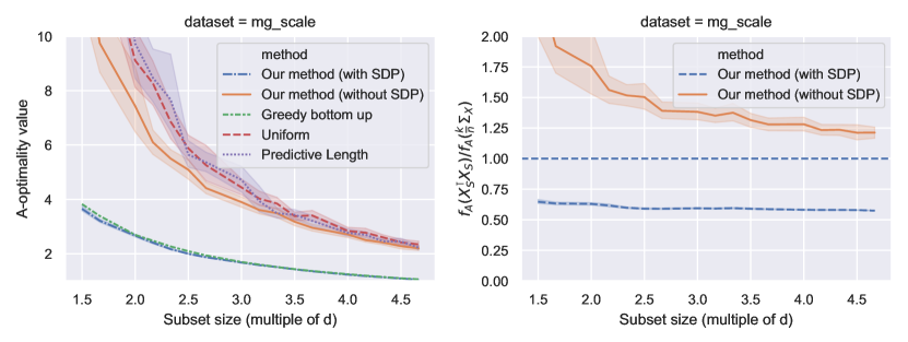
Figure 1: (left) A-optimality value obtained by the various methods on the mg_scale dataset [CL11] with prior precision $\mathbf{A}=10^{-5}\,\mathbf{I}$, (right) A-optimality value for our method (with and without SDP) divided by $f_{\mathbf{A}}(\frac{k}{n}\mathbf{\Sigma}_{\mathbf{X}})$, the baseline estimate suggested by Theorem 1.

Figure 1 (left) reveals that our method (without SDP) is superior to both uniform and predictive length sampling, producing designs which achieve lower $A$-optimality criteria values for all sample sizes. As Theorem 5 shows that our method (without SDP) only differs from uniform sampling by an additional DPP sample with controlled expected size (see Lemma 10), we may conclude that adding even a small DPP sample can improve a uniformly sampled design.

Consistent with prior observations [CR17a, WYS17], the greedy bottom up method achieves surprisingly good performance. However, if our method is used in conjunction with an SDP solution, then we are able to match and even slightly exceed the performance of the greedy bottom up method. Furthermore, the overall run-time costs (see Appendix C) between the two are comparable. As the majority of the runtime of our method (with SDP) is occupied by solving the SDP, an interesting future direction is to investigate alternative solvers such as interior point methods as well as terminating the solvers early once an approximate solution is reached.

Figure 1 (right) displays the ratio $f_{\mathbf{A}}(\mathbf{X}_{S}^{\scriptscriptstyle{\top}}\mathbf{X}_{S})\,/\,f_{\mathbf{A}}(\frac{k}{n}\mathbf{\Sigma}_{\mathbf{X}})$ for subsets returned by our method (with and without SDP). Note that the line for our method with SDP on Figure 1 (right) shows that the ratio never goes below 0.5, and we saw similar behavior across all examined datasets (see Appendix C). This evidence suggests that for many real datasets ${\textsc{OPT}_{k}}$ is within a small constant factor of $f_{\mathbf{A}}(\frac{k}{n}\mathbf{\Sigma}_{\mathbf{X}})$, matching the upper bound of Theorem 1.

Acknowledgements

MWM would like to acknowledge ARO, DARPA, NSF and ONR for providing partial support of this work. Also, MWM and MD thank the NSF for funding via the NSF TRIPODS program. The authors thank Uthaipon T. Tantipongpipat for valuable discussions.

Appendix A Properties of regularized DPPs

In this section we provide proofs omitted from Sections 3 and 4. We start with showing the fact that the regularized DPP distribution ${{\mathrm{DPP}}_{\!\mathrm{reg}}^{p}}(\mathbf{X},\mathbf{A})$ is a correlation DPP.

Lemma 14 (restated Lemma 8)

Given $\mathbf{X}$, $\mathbf{A}$, and $\mathbf{D}_{p}$ as in Theorem 5, we have

$${{\mathrm{DPP}}_{\!\mathrm{reg}}^{p}}(\mathbf{X},\mathbf{A})={{\mathrm{DPP}}_{\!\mathrm{cor}}}\big{(}\mathbf{D}_{p}+(\mathbf{I}-\mathbf{D}_{p})^{\nicefrac{{1}}{{2}}}\,\mathbf{D}_{p}^{\nicefrac{{1}}{{2}}}\mathbf{X}(\mathbf{A}+\mathbf{X}^{\scriptscriptstyle{\top}}\mathbf{D}_{p}\mathbf{X})^{-1}\mathbf{X}^{\scriptscriptstyle{\top}}\mathbf{D}_{p}^{\nicefrac{{1}}{{2}}}(\mathbf{I}-\mathbf{D}_{p})^{\nicefrac{{1}}{{2}}}\big{)}.$$

Proof  First, we show this under the invertibility assumptions of Lemma 7, i.e., given that $\mathbf{A}$ and $\mathbf{I}-\mathbf{D}_{p}$ are invertible. In this case ${{\mathrm{DPP}}_{\!\mathrm{reg}}^{p}}(\mathbf{X},\mathbf{A})={{\mathrm{DPP}}_{\!\mathrm{ens}}}(\mathbf{L})$, where

$$\mathbf{L}=\widetilde{\mathbf{D}}+\widetilde{\mathbf{D}}^{\nicefrac{{1}}{{2}}}\mathbf{X}\mathbf{A}^{-1}\mathbf{X}^{\scriptscriptstyle{\top}}\widetilde{\mathbf{D}}^{\nicefrac{{1}}{{2}}}\quad\text{ and }\quad\widetilde{\mathbf{D}}=\mathbf{D}_{p}(\mathbf{I}-\mathbf{D}_{p})^{-1}.$$ (6)

Converting this to a correlation kernel $\mathbf{K}$ and denoting $\widetilde{\mathbf{X}}=\mathbf{D}_{p}^{\nicefrac{{1}}{{2}}}\mathbf{X}$, we obtain

$$\mathbf{K} =\mathbf{I}-(\mathbf{I}+\mathbf{L})^{-1}$$

$$=\mathbf{I}-\big{(}\mathbf{I}+(\mathbf{I}-\mathbf{D}_{p})^{-1}\mathbf{D}_{p}+(\mathbf{I}-\mathbf{D}_{p})^{-\nicefrac{{1}}{{2}}}\widetilde{\mathbf{X}}\mathbf{A}^{-1}\widetilde{\mathbf{X}}^{\scriptscriptstyle{\top}}(\mathbf{I}-\mathbf{D}_{p})^{-\nicefrac{{1}}{{2}}}\big{)}^{-1}$$

$$=\mathbf{I}-\big{(}(\mathbf{I}-\mathbf{D}_{p})^{-1}+(\mathbf{I}-\mathbf{D}_{p})^{-\nicefrac{{1}}{{2}}}\widetilde{\mathbf{X}}\mathbf{A}^{-1}\widetilde{\mathbf{X}}^{\scriptscriptstyle{\top}}(\mathbf{I}-\mathbf{D}_{p})^{-\nicefrac{{1}}{{2}}}\big{)}^{-1}$$

$$=\mathbf{I}-(\mathbf{I}-\mathbf{D}_{p})^{\nicefrac{{1}}{{2}}}(\mathbf{I}+\widetilde{\mathbf{X}}\mathbf{A}^{-1}\widetilde{\mathbf{X}}^{\scriptscriptstyle{\top}})^{-1}(\mathbf{I}-\mathbf{D}_{p})^{\nicefrac{{1}}{{2}}}$$

$$\overset{(*)}{=}\mathbf{I}-(\mathbf{I}-\mathbf{D}_{p})^{\nicefrac{{1}}{{2}}}\big{(}\mathbf{I}-\widetilde{\mathbf{X}}\mathbf{A}^{-\nicefrac{{1}}{{2}}}(\mathbf{I}+\mathbf{A}^{-\nicefrac{{1}}{{2}}}\widetilde{\mathbf{X}}^{\scriptscriptstyle{\top}}\widetilde{\mathbf{X}}\mathbf{A}^{-\nicefrac{{1}}{{2}}})^{-1}\mathbf{A}^{-\nicefrac{{1}}{{2}}}\widetilde{\mathbf{X}}^{\scriptscriptstyle{\top}}\big{)}(\mathbf{I}-\mathbf{D}_{p})^{\nicefrac{{1}}{{2}}}$$

$$=\mathbf{I}-(\mathbf{I}-\mathbf{D}_{p})+(\mathbf{I}-\mathbf{D}_{p})^{\nicefrac{{1}}{{2}}}\widetilde{\mathbf{X}}(\mathbf{A}+\widetilde{\mathbf{X}}^{\scriptscriptstyle{\top}}\widetilde{\mathbf{X}})^{-1}\widetilde{\mathbf{X}}^{\scriptscriptstyle{\top}}(\mathbf{I}-\mathbf{D}_{p})^{\nicefrac{{1}}{{2}}}$$

$$=\mathbf{D}_{p}+(\mathbf{I}-\mathbf{D}_{p})^{\nicefrac{{1}}{{2}}}\widetilde{\mathbf{X}}(\mathbf{A}+\widetilde{\mathbf{X}}^{\scriptscriptstyle{\top}}\widetilde{\mathbf{X}})^{-1}\widetilde{\mathbf{X}}^{\scriptscriptstyle{\top}}(\mathbf{I}-\mathbf{D}_{p})^{\nicefrac{{1}}{{2}}},$$

where $(*)$ follows from Fact 2.16.19 in [Ber11]. Note that converting from $\mathbf{L}$ to $\mathbf{K}$ got rid of the inverses $\mathbf{A}^{-1}$ and $(\mathbf{I}-\mathbf{D}_{p})^{-1}$ appearing in (6). The intuition is that when $\mathbf{A}$ or $\mathbf{I}-\mathbf{D}_{p}$ is non-invertible, then ${{\mathrm{DPP}}_{\!\mathrm{reg}}^{p}}(\mathbf{X},\mathbf{A})$ is not an L-ensemble but it is still a correlation DPP. To show this, we use a limit argument. For $\epsilon\in[0,1]$, let $p_{\epsilon}=(1-\epsilon)p$ and $\mathbf{A}_{\epsilon}=\mathbf{A}+\epsilon\mathbf{I}$. Observe that if $\epsilon>0$ then $\mathbf{A}_{\epsilon}$ and $\mathbf{I}-\mathbf{D}_{p_{\epsilon}}$ are always invertible even if $\mathbf{A}$ and $\mathbf{I}-\mathbf{D}_{p}$ are not. Denote $\mathbf{K}_{\epsilon}$ as the above correlation kernel with $p$ replaced by $p_{\epsilon}$ and $\mathbf{A}$ replaced by $\mathbf{A}_{\epsilon}$. Note that all matrix operations defining kernel $\mathbf{K}_{\epsilon}$ are continuous w.r.t. $\epsilon\in[0,1]$, including the inverse, since $\mathbf{A}+\widetilde{\mathbf{X}}^{\scriptscriptstyle{\top}}\widetilde{\mathbf{X}}$ is assumed to be invertible. Therefore, the following equalities hold (with limits taken point-wise and $\epsilon>0$):

$${{\mathrm{DPP}}_{\!\mathrm{reg}}^{p}}(\mathbf{X},\mathbf{A})=\lim_{\epsilon\rightarrow 0}{{\mathrm{DPP}}_{\!\mathrm{reg}}^{p_{\epsilon}}}(\mathbf{X},\mathbf{A}_{\epsilon})=\lim_{\epsilon\rightarrow 0}{{\mathrm{DPP}}_{\!\mathrm{cor}}}(\mathbf{K}_{\epsilon})={{\mathrm{DPP}}_{\!\mathrm{cor}}}(\mathbf{K}),$$

where we did not have to assume invertibility of $\mathbf{A}$ or $\mathbf{I}-\mathbf{D}_{p}$.  
We now prove a lemma about combining a determinantal point process with Bernoulli sampling, which itself is a DPP with a diagonal correlation kernel.

Lemma 15 (restated Lemma 9)

Let $\mathbf{K}$ and $\mathbf{D}$ be $n\times n$ psd matrices with eigenvalues between 0 and 1, and assume that $\mathbf{D}$ is diagonal. If  $T\!\sim{{\mathrm{DPP}}_{\!\mathrm{cor}}}(\mathbf{K})$ and $R\sim{{\mathrm{DPP}}_{\!\mathrm{cor}}}(\mathbf{D})$, then

$$T\cup R\sim{{\mathrm{DPP}}_{\!\mathrm{cor}}}\big{(}\mathbf{D}+(\mathbf{I}-\mathbf{D})^{\nicefrac{{1}}{{2}}}\mathbf{K}(\mathbf{I}-\mathbf{D})^{\nicefrac{{1}}{{2}}}\big{)}.$$

Proof  For this proof we will use the shorthand $\mathbf{K}_{A}$ for $\mathbf{K}_{A,A}$. If $\mathbf{D}$ has no zeros on the diagonal then $\det(\mathbf{D}_{A})>0$ for all $A\subseteq[n]$ and

$$\mathrm{Pr}(A\subset T\cup R) =\sum_{B\subset A}\mathrm{Pr}(R\cap A=A\setminus B)\ \mathrm{Pr}(B\subseteq T)$$

$$=\sum_{B\subset A}\det(\mathbf{D}_{A\setminus B})\det\!\big{(}[\mathbf{I}-\mathbf{D}]_{B}\big{)}\,\det(\mathbf{K}_{B})$$

$$=\sum_{B\subset A}\det(\mathbf{D}_{A\setminus B})\det\!\Big{(}\big{[}(\mathbf{I}-\mathbf{D})^{\nicefrac{{1}}{{2}}}\mathbf{K}(\mathbf{I}-\mathbf{D})^{\nicefrac{{1}}{{2}}}\big{]}_{B}\Big{)}$$

$$=\det(\mathbf{D}_{A})\sum_{B\subset A}\det\!\Big{(}\big{[}\mathbf{D}^{-\nicefrac{{1}}{{2}}}(\mathbf{I}-\mathbf{D})^{\nicefrac{{1}}{{2}}}\mathbf{K}(\mathbf{I}-\mathbf{D})^{\nicefrac{{1}}{{2}}}\mathbf{D}^{-\nicefrac{{1}}{{2}}}\big{]}_{B}\Big{)}$$

$$\overset{(*)}{=}\det(\mathbf{D}_{A})\det\!\Big{(}\mathbf{I}+\big{[}\mathbf{D}^{-\nicefrac{{1}}{{2}}}(\mathbf{I}-\mathbf{D})^{\nicefrac{{1}}{{2}}}\mathbf{K}(\mathbf{I}-\mathbf{D})^{\nicefrac{{1}}{{2}}}\mathbf{D}^{-\nicefrac{{1}}{{2}}}\big{]}_{A}\Big{)}$$

$$=\det\!\Big{(}\big{[}\mathbf{D}+(\mathbf{I}-\mathbf{D})^{\nicefrac{{1}}{{2}}}\mathbf{K}(\mathbf{I}-\mathbf{D})^{\nicefrac{{1}}{{2}}}\big{]}_{A}\Big{)},$$

where $(*)$ follows from a standard determinantal identity used to compute the L-ensemble partition function [KT12, Theorem 2.1]. If $\mathbf{D}$ has zeros on the diagonal, a similar limit argument as in Lemma 8 with $\mathbf{D}_{\epsilon}=\mathbf{D}+\epsilon\,\mathbf{I}$ holds.  
Next, we give a bound on the expected size of a regularized DPP.

Lemma 16 (restated Lemma 10)

Given any $\mathbf{X}\in\mathbb{R}^{n\times d}$, $p\in[0,1]^{n}$ and a psd matrix $\mathbf{A}$ s.t. $\sum_{i}p_{i}\mathbf{x}_{i}\mathbf{x}_{i}^{\scriptscriptstyle{\top}}\!+\mathbf{A}$ is full rank, let $S=T\cup\{i:b_{i}=1\}\sim{{\mathrm{DPP}}_{\!\mathrm{reg}}^{p}}(\mathbf{X},\mathbf{A})$ be defined as in Theorem 5. Then

$$\mathbb{E}\big{[}|S|\big{]}\leq\mathbb{E}\big{[}|T|\big{]}+\mathbb{E}\Big{[}\sum_{i}b_{i}\Big{]}=d_{\mathbf{A}}\Big{(}\sum_{i}p_{i}\mathbf{x}_{i}\mathbf{x}_{i}^{\scriptscriptstyle{\top}}\Big{)}+\sum_{i}p_{i}.$$

Proof  For correlation kernels it is known that the expected size of ${{\mathrm{DPP}}_{\!\mathrm{cor}}}(\mathbf{K})$ is $\mathrm{tr}(\mathbf{K})$. Thus, using $\mathbf{D}_{p}=\operatorname*{\mathop{\mathrm{diag}}}(p)$, we can invoke Lemma 8 to obtain

$$\mathbb{E}\big{[}|S|\big{]} =\mathrm{tr}\big{(}\mathbf{D}_{p}+(\mathbf{I}-\mathbf{D}_{p})^{\nicefrac{{1}}{{2}}}\,\mathbf{D}_{p}^{\nicefrac{{1}}{{2}}}\mathbf{X}(\mathbf{A}+\mathbf{X}^{\scriptscriptstyle{\top}}\mathbf{D}_{p}\mathbf{X})^{-1}\mathbf{X}^{\scriptscriptstyle{\top}}\mathbf{D}_{p}^{\nicefrac{{1}}{{2}}}(\mathbf{I}-\mathbf{D}_{p})^{\nicefrac{{1}}{{2}}}\big{)}$$

$$\leq\mathrm{tr}(\mathbf{D}_{p})+\mathrm{tr}\big{(}\mathbf{D}_{p}^{\nicefrac{{1}}{{2}}}\mathbf{X}(\mathbf{A}+\mathbf{X}^{\scriptscriptstyle{\top}}\mathbf{D}_{p}\mathbf{X})^{-1}\mathbf{X}^{\scriptscriptstyle{\top}}\mathbf{D}_{p}^{\nicefrac{{1}}{{2}}}\big{)}$$

$$=\mathrm{tr}(\mathbf{D}_{p})+\mathrm{tr}\big{(}\mathbf{X}^{\scriptscriptstyle{\top}}\mathbf{D}_{p}\mathbf{X}(\mathbf{A}+\mathbf{X}^{\scriptscriptstyle{\top}}\mathbf{D}_{p}\mathbf{X})^{-1}\big{)}=\mathrm{tr}(\mathbf{D}_{p})+d_{\mathbf{A}}(\mathbf{X}^{\scriptscriptstyle{\top}}\mathbf{D}_{p}\mathbf{X}),$$

from which the claim follows.  
Next, we show two expectation inequalities for the matrix inverse and matrix determinant.

Lemma 17 (restated Lemma 11)

Whenever $S\sim{{\mathrm{DPP}}_{\!\mathrm{reg}}^{p}}(\mathbf{X},\mathbf{A})$ is a well-defined distribution it holds that

$$\mathbb{E}\Big{[}\big{(}\mathbf{X}_{S}^{\scriptscriptstyle{\top}}\mathbf{X}_{S}+\mathbf{A}\big{)}^{-1}\Big{]} \preceq\Big{(}\sum_{i}p_{i}\mathbf{x}_{i}\mathbf{x}_{i}^{\scriptscriptstyle{\top}}+\mathbf{A}\Big{)}^{-1},$$ (7)

$$\mathbb{E}\Big{[}\det\!\big{(}\mathbf{X}_{S}^{\scriptscriptstyle{\top}}\mathbf{X}_{S}+\mathbf{A}\big{)}^{-1}\Big{]} \leq\det\!\Big{(}\sum_{i}p_{i}\mathbf{x}_{i}\mathbf{x}_{i}^{\scriptscriptstyle{\top}}+\mathbf{A}\Big{)}^{-1}.$$ (8)

Proof  For a square matrix $\mathbf{M}$, define its adjugate, denoted $\operatorname{\textnormal{adj}}(\mathbf{M})$, as a matrix whose $i,j$-th entry is $(-1)^{i+j}\det(\mathbf{M}_{-j,-i})$, where $\mathbf{M}_{-j,-i}$ is the matrix $\mathbf{M}$ without $j$th row and $i$th column. If $\mathbf{M}$ is invertible, then $\operatorname{\textnormal{adj}}(\mathbf{M})=\det(\mathbf{M})\mathbf{M}^{-1}$. Now, let $b_{i}\sim\mathrm{Bernoulli}(p_{i})$ be independent random variables. As seen in previous section, the identity $\mathbb{E}[\det(\sum_{i}b_{i}\mathbf{x}_{i}\mathbf{x}_{i}^{\scriptscriptstyle{\top}}+\mathbf{A})]=\det(\sum_{i}p_{i}\mathbf{x}_{i}\mathbf{x}_{i}^{\scriptscriptstyle{\top}}+\mathbf{A})$ gives us the normalization constant for ${{\mathrm{DPP}}_{\!\mathrm{reg}}^{p}}(\mathbf{X},\mathbf{A})$. Moreover, as noted in a different context by [DM19], when applied entrywise to the adjugate matrix, this identity implies that $\mathbb{E}[\operatorname{\textnormal{adj}}(\sum_{i}b_{i}\mathbf{x}_{i}\mathbf{x}_{i}^{\scriptscriptstyle{\top}}+\mathbf{A})]=\operatorname{\textnormal{adj}}(\sum_{i}p_{i}\mathbf{x}_{i}\mathbf{x}_{i}^{\scriptscriptstyle{\top}}+\mathbf{A})$. Let $\mathcal{I}$ denote the set of all subsets $S\subseteq[n]$ such that $\mathbf{X}_{S}^{\scriptscriptstyle{\top}}\mathbf{X}_{S}+\mathbf{A}$ is invertible. We have

$$\mathbb{E}\Big{[}\big{(}\mathbf{X}_{S}^{\scriptscriptstyle{\top}}\mathbf{X}_{S}+\mathbf{A}\big{)}^{-1}\Big{]} =\sum_{S\in\mathcal{I}}\big{(}\mathbf{X}_{S}^{\scriptscriptstyle{\top}}\mathbf{X}_{S}+\mathbf{A}\big{)}^{-1}\frac{\det(\mathbf{X}_{S}^{\scriptscriptstyle{\top}}\mathbf{X}_{S}+\mathbf{A})}{\det(\sum_{i}p_{i}\mathbf{x}_{i}\mathbf{x}_{i}^{\scriptscriptstyle{\top}}+\mathbf{A})}\ \prod_{i\in S}p_{i}\prod_{i\not\in S}(1-p_{i})$$

$$=\sum_{S\in\mathcal{I}}\frac{\operatorname{\textnormal{adj}}(\mathbf{X}_{S}^{\scriptscriptstyle{\top}}\mathbf{X}_{S}+\mathbf{A}\big{)}}{\det(\sum_{i}p_{i}\mathbf{x}_{i}\mathbf{x}_{i}^{\scriptscriptstyle{\top}}+\mathbf{A})}\ \prod_{i\in S}p_{i}\prod_{i\not\in S}(1-p_{i})$$

$$\preceq\sum_{S\subseteq[n]}\frac{\operatorname{\textnormal{adj}}(\mathbf{X}_{S}^{\scriptscriptstyle{\top}}\mathbf{X}_{S}+\mathbf{A}\big{)}}{\det(\sum_{i}p_{i}\mathbf{x}_{i}\mathbf{x}_{i}^{\scriptscriptstyle{\top}}+\mathbf{A})}\ \prod_{i\in S}p_{i}\prod_{i\not\in S}(1-p_{i})$$

$$=\frac{\mathbb{E}\big{[}\!\operatorname{\textnormal{adj}}(\sum_{i}b_{i}\mathbf{x}_{i}\mathbf{x}_{i}^{\scriptscriptstyle{\top}}+\mathbf{A})\big{]}}{\det(\sum_{i}p_{i}\mathbf{x}_{i}\mathbf{x}_{i}^{\scriptscriptstyle{\top}}+\mathbf{A})}$$

$$=\frac{\operatorname{\textnormal{adj}}(\sum_{i}p_{i}\mathbf{x}_{i}\mathbf{x}_{i}^{\scriptscriptstyle{\top}}+\mathbf{A})}{\det(\sum_{i}p_{i}\mathbf{x}_{i}\mathbf{x}_{i}^{\scriptscriptstyle{\top}}+\mathbf{A})}=\Big{(}\sum_{i}p_{i}\mathbf{x}_{i}\mathbf{x}_{i}^{\scriptscriptstyle{\top}}+\mathbf{A}\Big{)}^{-1}.$$

Note that if $\mathcal{I}$ contains all subsets of $[n]$, for example when $\mathbf{A}\succ\mathbf{0}$, then the inequality turns into equality. Thus, we showed (7), and (8) follows even more easily:

$$\mathbb{E}\Big{[}\!\det\!\big{(}\mathbf{X}_{S}^{\scriptscriptstyle{\top}}\mathbf{X}_{S}+\mathbf{A}\big{)}^{-1}\Big{]} =\sum_{S\in\mathcal{I}}\frac{1}{\det(\sum_{i}p_{i}\mathbf{x}_{i}\mathbf{x}_{i}^{\scriptscriptstyle{\top}}+\mathbf{A})}\ \prod_{i\in S}p_{i}\prod_{i\not\in S}(1-p_{i})\leq\det\!\Big{(}\sum_{i}p_{i}\mathbf{x}_{i}\mathbf{x}_{i}^{\scriptscriptstyle{\top}}\Big{)}^{\!-1}\!,$$

where the equality holds if $\mathcal{I}$ consists of all subsets of $[n]$.  

Appendix B Comparison of different effective dimensions

In this section we compare the two notions of effective dimension for Bayesian experimental design considered in this work. Here, we let $\mathbf{X}$ be the full $n\times d$ design matrix and use $k$ to denote the desired subset size. Recall that the effective dimension is defined as a function of the data covariance matrix $\mathbf{\Sigma}_{\mathbf{X}}=\mathbf{X}^{\scriptscriptstyle{\top}}\mathbf{X}$ and the prior precision matrix $\mathbf{A}$: It is given by $d_{\mathbf{A}}=\mathrm{tr}\big{(}\mathbf{\Sigma}_{\mathbf{X}}(\mathbf{A}+\mathbf{\Sigma}_{\mathbf{X}})^{-1}\big{)}$. In [DW18b] it was suggested that $d_{\mathbf{A}}$ should also be used as the effective dimension for the experimental design problem. Our results suggest it may not reflect the true degrees of freedom of the problem because it does not scale with subset size $k$. Instead we propose to use the scaled effective dimension $d_{\frac{n}{k}\!\mathbf{A}}$. Thus, the two definitions we are comparing can be summarized as follows:

Full effective dimension

$d_{\mathbf{A}}=\mathrm{tr}\big{(}\mathbf{\Sigma}_{\mathbf{X}}(\mathbf{A}+\mathbf{\Sigma}_{\mathbf{X}})^{-1}\big{)}$,

Scaled effective dimension

$d_{\frac{n}{k}\!\mathbf{A}}=\mathrm{tr}\big{(}\mathbf{\Sigma}_{\mathbf{X}}(\tfrac{n}{k}\mathbf{A}+\mathbf{\Sigma}_{\mathbf{X}})^{-1}\big{)}$.

Here, we demonstrate that these two effective dimensions can be very different for some matrices and quite similar on others. For simplicity, we consider two diagonal data covariance matrices as our examples: identity covariance, $\mathbf{\Sigma}_{1}=\mathbf{I}$, and an approximately low-rank covariance, $\mathbf{\Sigma}_{2}=(1-\epsilon)\frac{d}{s}\mathbf{I}_{S}+\epsilon\mathbf{I}$, where $\mathbf{I}_{S}$ is the diagonal matrix with ones on the entries indexed by subset $S\subseteq[d]$ of size $s<d$ and zeros everywhere else. The second matrix is scaled in such way so that $\mathrm{tr}(\mathbf{\Sigma}_{1})=\mathrm{tr}(\mathbf{\Sigma}_{2})$. We use $d=100$, $s=10$ and $\epsilon=10^{-2}$. The prior precision matrix is $\mathbf{A}=10^{-2}\,\mathbf{I}$. Figure 2 plots the scaled effective dimension $d_{\frac{n}{k}\!\mathbf{A}}$ as a function of $k$, against the full effective dimension for both examples. Unsurprisingly, for the identity covariance the full effective dimension is almost $d$, and the scaled effective dimension goes up very quickly to match it. On the other hand, for the approximately low-rank covariance, $d_{\mathbf{A}}\approx 55$ is considerably less then $d=100$. Interestingly, the gap between the $d_{\frac{n}{k}\!\mathbf{A}}$ and $d_{\mathbf{A}}$ for moderately small values of $k$ is even bigger. Our theory suggests that $d_{\frac{n}{k}\!\mathbf{A}}$ is a valid indicator of Bayesian degrees of freedom when $k\geq C\cdot d_{\frac{n}{k}\!\mathbf{A}}$ for some small constant $C$ (Theorem 1 has $C=4$, but we believe this can be improved to $1$). While for the identity covariance the condition $k\geq d_{\frac{n}{k}\!\mathbf{A}}$ is almost equivalent to $k\geq d_{\mathbf{A}}$, in the approximately low-rank case, $k\geq d_{\frac{n}{k}\!\mathbf{A}}$ holds for $k$ as small as 20, much less than $d_{\mathbf{A}}$.

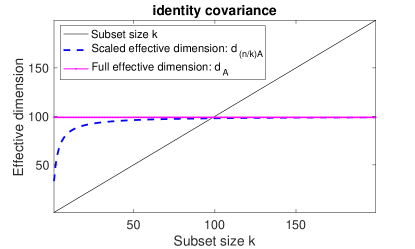
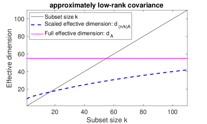
Figure 2: Scaled effective dimension compared to the full effective dimension for two diagonal data covariance matrices, with $\mathbf{A}=10^{-2}\,\mathbf{I}$.

Appendix C Additional details for the experiments

This section presents additional details and experimental results omitted from the main body of the paper. In addition to the mg_scale dataset presented in Section 5, we also benchmarked on three other data sets described in Table 2.

Table 2: [CL11] datasets used in experiments

	mg_scale	bodyfat_scale	mpg_scale	housing_scale
$n$	1385	252	392	506
$d$	6	14	7	13

The A-optimality values obtained are illustrated in Figure 3. The general trend observed in Section 5 of our method (without SDP) outperforming independent sampling methods (uniform and predictive length) and our method (with SDP) matching the performance of the greedy bottom up method continues to hold across the additional datasets considered.

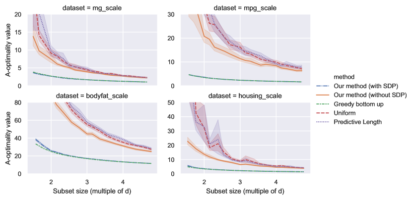
Figure 3: A-optimality values achieved by the methods compared. In all cases considered, we found our method (without SDP) to be superior to independent sampling methods like uniform and predictive length sampling. After paying the price to solve an SDP, our method (with SDP) is able to consistently match the performance of a greedy method which has been noted [CR17a] to work well empirically.

The relative ranking and overall order of magnitude differences between runtimes (Figure 4) are also similar across the various datasets. An exception to the rule is on mg_scale, where we see that our method (without SDP) costs more than the greedy method (whereas everywhere else it costs less).

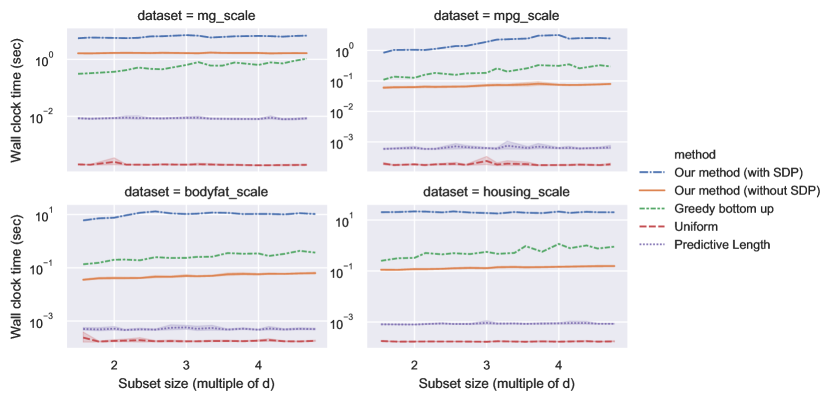
Figure 4: Runtimes of the methods compared. Our method (without SDP) is within an order of magnitude of greedy bottom up and faster in 3 out of 4 cases. The gap between our method with and without SDP is attributable to the SDP solver, making investigation of more efficient solvers and approximate solutions an interesting direction for future work.

The claim that $f_{\mathbf{A}}(\frac{k}{n}\mathbf{\Sigma}_{\mathbf{X}})$ is an appropriate quantity to summarize the contribution of problem-dependent factors on the performance of Bayesian A-optimal designs is further evidenced in Figure 5. Here, we see that after normalizing the A-optimality values by this quantity, the remaining quantities are all on the same scale and close to $1$.

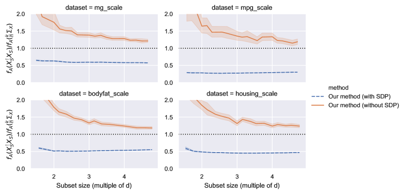
Figure 5: The ratio controlled by Lemma 13. This ratio converges to $1$ as $k\to n$ and is close to $1$ across all real world datasets, suggesting that $f_{\mathbf{A}}(\frac{k}{n}\mathbf{\Sigma}_{\mathbf{X}})$ is an appropriate problem-dependent scale for Bayesian A-optimal experimental design.

References

[AB13]
Haim Avron and Christos Boutsidis.
Faster subset selection for matrices and applications.
SIAM Journal on Matrix Analysis and Applications,
34(4):1464–1499, 2013.
[AM15]
Ahmed El Alaoui and Michael W. Mahoney.
Fast randomized kernel ridge regression with statistical guarantees.
In Proceedings of the 28th International Conference on Neural
Information Processing Systems, pages 775–783, Montreal, Canada, December
2015.