Bayesian multi-parameter quantum metrology with limited data

Abstract

A longstanding problem in quantum metrology is how to extract as much information as possible in realistic scenarios with not only multiple unknown parameters, but also limited measurement data and some degree of prior information. Here we present a practical solution to this: we derive a new Bayesian multi-parameter quantum bound, construct the optimal measurement when our bound can be saturated for a single shot and consider experiments involving a repeated sequence of these measurements. Our method properly accounts for the number of measurements and the degree of prior information, and we illustrate our ideas with a qubit sensing network and a model for phase imaging, clarifying the non-asymptotic role of local and global schemes. Crucially, our technique is a powerful way of implementing quantum protocols in a wide range of practical scenarios that tools such as the Helstrom and Holevo Cramér-Rao bounds cannot normally access.

I Introduction

Real-world applications typically give rise to estimation problems with several unknown pieces of information. For instance, we may wish to determine the range and velocity of a moving object Zhuang et al. (2017), quantify phases and phase diffusion Vidrighin et al. (2014); Szczykulska et al. (2017), reconstruct an image Humphreys et al. (2013); Knott et al. (2016); Zhang and Chan (2017), estimate the components of some field Baumgratz and Datta (2016), assess spatial deformations in a grid of sources Sidhu and Kok (2017, 2018) or use quantum networks to implement distributed sensing protocols Proctor et al. (2017, 2018); Ge et al. (2018); Eldredge et al. (2018); Altenburg and Wölk (2018); Qian et al. (2019); Guo et al. (2019). In this context, many results in existing literature rely on the multi-parameter Cramér-Rao bound and its quantum extension by Helstrom Helstrom (1976); Paris (2009); Szczykulska et al. (2016); Ragy et al. (2016); Pezzè et al. (2017); Liu et al. (2019).

This framework is powerful because sometimes there is a quantum strategy for which the classical and quantum versions of the bound coincide Ragy et al. (2016); Pezzè et al. (2017) (e.g., for commuting generators and pure states Ragy et al. (2016); Pezzè et al. (2017); Proctor et al. (2017)). However, to exploit it one first needs to reach the classical bound. One possibility is assuming locally unbiased estimators Fraser (1964), which may be reasonable for large prior information Hall and Wiseman (2012); Demkowicz-Dobrzański et al. (2015); Haase et al. (2018), although in general many repetitions of the experiment are required to approach the bound Kay (1993). While this may generate fundamental results locally or at least asymptotically, the fact that the measurement data can be limited in practice (e.g., Berchera and Degiovanni (2019); Polino et al. (2019)) and that our prior knowledge may be moderate motivates the search for a more generally applicable strategy Rubio and Dunningham (2019); Rubio (2020).

Current research is exploring the Holevo Cramér-Rao bound Holevo (2011); Ragy et al. (2016); Yang et al. (2019); Carollo et al. (2019); Tsang (2019a); Albarelli et al. (2019a); Vidarte (2019); Albarelli et al. (2020, 2019b); Sidhu et al. (2019), which is more informative than Helstrom’s counterpart (albeit moderately Carollo et al. (2019); Albarelli et al. (2019a); Tsang (2019a)) when the latter produces incompatible estimators. Unfortunately, this bound is still restricted by either local unbiasedness or, generally, the requirement of an asymptotically large number of copies of the scheme Holevo (2011); Yang et al. (2019); Ragy et al. (2016); Tsang (2019a). Hence, it lacks the type of generality that we seek.

Instead, we recall that the fundamental equations that the optimal quantum strategy must satisfy for a single or several copies have been known since the Bayesian works of Helstrom, Holevo, Personick, Yuen and others Personick (1971); Helstrom (1976); Helstrom and Kennedy (1974); Holevo (1973a, b); Yuen and Lax (1973), and that the Bayesian framework does provide the tools for scenarios with limited data where the prior information plays an active role Jaynes (2003); Rubio (2020). A recent review of this formalism, including both classical and quantum aspects, can be found in chapter 3 of Rubio (2020).

Except for a few cases such as those admitting covariant measurements D’Ariano et al. (1998); Macchiavello (2003); Chiribella et al. (2005); Holevo (2011); Demkowicz-Dobrzański et al. (2015), solving these equations exactly is challenging Helstrom (1976), and the known solutions usually assume no a priori knowledge, with exceptions such as the single-parameter work Demkowicz-Dobrzański (2011). Fortunately, our single-parameter proposal in Rubio and Dunningham (2019) already shows that this formalism can be exploited in a less general but more practical way. In particular, if using the square error is justified (as it is for moderate prior knowledge Demkowicz-Dobrzański et al. (2015); Rubio et al. (2018); Friis et al. (2017); Rubio and Dunningham (2019); Rubio (2020)), then we may calculate the single-shot optimal quantum strategy Personick (1971); Macieszczak et al. (2014) and repeat it as many times as the application at hand demands or allows for Rubio and Dunningham (2019). This generates uncertainties that have been optimised in a shot-by-shot fashion, and that sometimes recover the single-parameter quantum Cramér-Rao bound asymptotically as a limiting case Rubio (2020).

The aim of this paper is to construct a multi-parameter version of the efficient shot-by-shot technique described above, a step that will generalise and take quantum metrology to a new level by providing the means of addressing practical problems beyond the scope of the Helstrom and Holevo Cramér-Rao bounds. First we derive a new multi-parameter quantum bound for the quadratic error in Sec. II. This bound can incorporate prior information explicitly without imposing a particular form for the prior probability, and its derivation does not involve unbiasedness conditions. We then study its potential saturability for a single shot, and we discuss how and under which circumstances we can adapt this result to exploit it in strategies where the same experiment is repeated several times. To illustrate our ideas, in Sec. III we apply our new multi-parameter technique to a qubit sensing network and a discrete model for phase imaging, and we analyse the role of local and global sensing protocols (in the sense of Proctor et al. (2017, 2018)) when the scheme operates in the non-asymptotic regime of a finite and possibly small number of experiments. Finally, the merits and potential extensions of our results are discussed in Sec. IV.

Note added. After completion of the first version of this work (see ), Sidhu and Kok Sidhu and Kok (2020) arrived at the quantum bound in Sec. II.1 independently by using a geometric approach. In addition, a version of the same result and a simplification for Gaussian priors was later discussed by Demkowicz-Dobrzański et al. in their review Demkowicz-Dobrzański et al. (2020). The interested readers will find in these works other perspectives that complement our findings, which here are instead understood in terms of the non-asymptotic version of quantum metrology developed in Rubio (2020).

II A new multi-parameter technique

II.1 Derivation of the bound

Suppose we encode the unknown parameters $\bm{\theta}=(\theta_{1},\cdots,\theta_{d})$ in the probe state $\rho_{0}$, so that the transformed state is $\rho(\bm{\theta})$, and that we perform a single measurement $E(m)$ with outcome $m$. Then the likelihood is $p(m|\bm{\theta})=\mathrm{Tr}[E(m)\rho(\bm{\theta})]$, and by combining it with the prior $p(\bm{\theta})$ into the joint probability $p(\bm{\theta},m)=p(\bm{\theta})p(m|\bm{\theta})$ we can construct the uncertainty

$$\bar{\epsilon}_{\mathrm{mse}}=\sum_{i=1}^{d}w_{i}\int d\bm{\theta}dm\leavevmode\nobreak\ p(\bm{\theta},m)\left[g_{i}(m)-\theta_{i}\right]^{2},$$ (1)

where $g_{i}(m)$ is the estimator for the $i$-th parameter, $w_{i}\geqslant 0$ indicates its relative importance Proctor et al. (2017) and $\sum_{i=1}^{d}w_{i}=1$.

Let us rewrite Eq. (1) as $\bar{\epsilon}_{\mathrm{mse}}=\mathrm{Tr}[\mathcal{W}\Sigma_{\mathrm{mse}}]$, where $\mathcal{W}=\mathrm{diag}(w_{1},\dots,w_{d})$ and

$$\Sigma_{\mathrm{mse}}=\int d\bm{\theta}dm\leavevmode\nobreak\ p(\bm{\theta},m)\left[\bm{g}(m)-\bm{\theta}\right]\left[\bm{g}(m)-\bm{\theta}\right]^{\mathchoice{\raisebox{0.0pt}{$\displaystyle\intercal$}}{\raisebox{0.0pt}{$\textstyle\intercal$}}{\raisebox{0.0pt}{$\scriptstyle\intercal$}}{\raisebox{0.0pt}{$\scriptscriptstyle\intercal$}}},$$ (2)

and with $\bm{g}(m)=(g_{1}(m),\dots,g_{d}(m))$. The first step is performing a classical optimisation over all possible estimators. We start by constructing the scalar

$$\bm{u}^{\mathchoice{\raisebox{0.0pt}{$\displaystyle\intercal$}}{\raisebox{0.0pt}{$\textstyle\intercal$}}{\raisebox{0.0pt}{$\scriptstyle\intercal$}}{\raisebox{0.0pt}{$\scriptscriptstyle\intercal$}}}\Sigma_{\mathrm{mse}}\bm{u}=\int d\bm{\theta}dm\leavevmode\nobreak\ p(\bm{\theta},m)\left[g_{u}(m)-\theta_{u}\right]^{2},$$ (3)

with $g_{u}(m)=\bm{u}^{\mathchoice{\raisebox{0.0pt}{$\displaystyle\intercal$}}{\raisebox{0.0pt}{$\textstyle\intercal$}}{\raisebox{0.0pt}{$\scriptstyle\intercal$}}{\raisebox{0.0pt}{$\scriptscriptstyle\intercal$}}}\bm{g}(m)=\bm{g}^{\mathchoice{\raisebox{0.0pt}{$\displaystyle\intercal$}}{\raisebox{0.0pt}{$\textstyle\intercal$}}{\raisebox{0.0pt}{$\scriptstyle\intercal$}}{\raisebox{0.0pt}{$\scriptscriptstyle\intercal$}}}(m)\hskip 1.49994pt\bm{u}$, $\theta_{u}=\bm{u}^{\mathchoice{\raisebox{0.0pt}{$\displaystyle\intercal$}}{\raisebox{0.0pt}{$\textstyle\intercal$}}{\raisebox{0.0pt}{$\scriptstyle\intercal$}}{\raisebox{0.0pt}{$\scriptscriptstyle\intercal$}}}\bm{\theta}=\bm{\theta}^{\mathchoice{\raisebox{0.0pt}{$\displaystyle\intercal$}}{\raisebox{0.0pt}{$\textstyle\intercal$}}{\raisebox{0.0pt}{$\scriptstyle\intercal$}}{\raisebox{0.0pt}{$\scriptscriptstyle\intercal$}}}\bm{u}$ and $\bm{u}$ being an arbitrary real vector. If we look at $\bm{u}^{\mathchoice{\raisebox{0.0pt}{$\displaystyle\intercal$}}{\raisebox{0.0pt}{$\textstyle\intercal$}}{\raisebox{0.0pt}{$\scriptstyle\intercal$}}{\raisebox{0.0pt}{$\scriptscriptstyle\intercal$}}}\Sigma_{\mathrm{mse}}\bm{u}$ as a functional of $g_{u}(m)$ Jaynes (2003); Rubio et al. (2018), that is, $\bm{u}^{\mathchoice{\raisebox{0.0pt}{$\displaystyle\intercal$}}{\raisebox{0.0pt}{$\textstyle\intercal$}}{\raisebox{0.0pt}{$\scriptstyle\intercal$}}{\raisebox{0.0pt}{$\scriptscriptstyle\intercal$}}}\Sigma_{\mathrm{mse}}\bm{u}=\epsilon\left[g_{u}(m)\right]$, then we can formulate the variational problem

$$\delta\epsilon\left[g_{u}(m)\right]=\delta\int dm\leavevmode\nobreak\ \mathcal{L}\left[m,g_{u}(m)\right]=0,$$ (4)

with $\mathcal{L}\left[m,g_{u}(m)\right]=\int d\bm{\theta}p(\bm{\theta},m)\left[g_{u}(m)-\theta_{u}\right]^{2}$. Its solution, which we revisit in Appendix A, is $g_{u}(m)=\int d\bm{\theta}p(\bm{\theta}|m)\theta_{u}$, where $p(\bm{\theta}|m)\propto p(\bm{\theta})p(m|\bm{\theta})$ is the posterior probability.

The previous calculation implies that the vector estimator that makes the uncertainty extremal is $\bm{g}(m)=\int d\bm{\theta}p(\bm{\theta}|m)\bm{\theta}$, and this is precisely the solution that is known to achieve the minimum matrix error (see Kay (1993) and Appendix A). Hence, we have that $\bm{u}^{\mathchoice{\raisebox{0.0pt}{$\displaystyle\intercal$}}{\raisebox{0.0pt}{$\textstyle\intercal$}}{\raisebox{0.0pt}{$\scriptstyle\intercal$}}{\raisebox{0.0pt}{$\scriptscriptstyle\intercal$}}}\Sigma_{\mathrm{mse}}\bm{u}\geqslant\bm{u}^{\mathchoice{\raisebox{0.0pt}{$\displaystyle\intercal$}}{\raisebox{0.0pt}{$\textstyle\intercal$}}{\raisebox{0.0pt}{$\scriptstyle\intercal$}}{\raisebox{0.0pt}{$\scriptscriptstyle\intercal$}}}\Sigma_{c}\bm{u}$ after introducing $\bm{g}(m)=\int d\bm{\theta}p(\bm{\theta}|m)\bm{\theta}$ in Eq. (3), where

$$\bm{u}^{\mathchoice{\raisebox{0.0pt}{$\displaystyle\intercal$}}{\raisebox{0.0pt}{$\textstyle\intercal$}}{\raisebox{0.0pt}{$\scriptstyle\intercal$}}{\raisebox{0.0pt}{$\scriptscriptstyle\intercal$}}}\Sigma_{c}\bm{u}=\int d\bm{\theta}p(\bm{\theta})\theta_{u}^{2}-\int dm\frac{\left[\int d\bm{\theta}p(\bm{\theta})p(m|\bm{\theta})\theta_{u}\right]^{2}}{\int d\bm{\theta}p(\bm{\theta})p(m|\bm{\theta})}.$$ (5)

Next we examine the quantum part of the problem. By inserting $p(m|\bm{\theta})=\mathrm{Tr}[E(m)\rho(\bm{\theta})]$ in Eq. (5),

$$\bm{u}^{\mathchoice{\raisebox{0.0pt}{$\displaystyle\intercal$}}{\raisebox{0.0pt}{$\textstyle\intercal$}}{\raisebox{0.0pt}{$\scriptstyle\intercal$}}{\raisebox{0.0pt}{$\scriptscriptstyle\intercal$}}}\Sigma_{c}\bm{u}=\int d\bm{\theta}p(\bm{\theta})\theta_{u}^{2}-\int dm\frac{\mathrm{Tr}\left[E(m)\bar{\rho}_{u}\right]^{2}}{\mathrm{Tr}\left[E(m)\rho\right]},$$ (6)

where $\rho=\int d\bm{\theta}p(\bm{\theta})\rho(\bm{\theta})$ and $\bar{\rho}_{u}=\int d\bm{\theta}p(\bm{\theta})\rho(\bm{\theta})\theta_{u}$. Remarkably, the second term is formally analogous to the result of applying the Born rule to the expression for the classical Fisher information . This suggests the possibility of bounding it with a procedure similar to the proof of the Braunstein-Caves inequality Braunstein and Caves (1994); Genoni et al. (2008).

Following this analogy we introduce the Bayesian counterpart of the equation for the symmetric logarithmic derivative , i.e., $S_{u}\rho+\rho S_{u}=2\bar{\rho}_{u}$. This allows us to manipulate the second term in Eq. (6), which we denote by $B_{u}$, as

$$B_{u} =\int dm\left(\frac{\mathrm{Re}\left\{\mathrm{Tr}\left[E(m)S_{u}\rho\right]\right\}}{\sqrt{\mathrm{Tr}\left[E(m)\rho\right]}}\right)^{2}$$

$$\leqslant\int dm\leavevmode\nobreak\ \absolutevalue{\frac{\mathrm{Tr}\left[E(m)S_{u}\rho\right]}{\sqrt{\mathrm{Tr}\left[E(m)\rho\right]}}}^{2}$$

$$=\int dm\leavevmode\nobreak\ \absolutevalue{\mathrm{Tr}\left[\frac{\rho^{\frac{1}{2}}E(m)^{\frac{1}{2}}}{\sqrt{\mathrm{Tr}\left[E(m)\rho\right]}}E(m)^{\frac{1}{2}}S_{u}\rho^{\frac{1}{2}}\right]}^{2}$$

$$\leqslant\int dm\leavevmode\nobreak\ \mathrm{Tr}\left[E(m)S_{u}\rho S_{u}\right]=\mathrm{Tr}\left[\rho S_{u}^{2}\right]\equiv\mathcal{K}_{u},$$ (7)

having used the Cauchy-Schwarz inequality $|\mathrm{Tr}[X^{\dagger}Y]|^{2}\leqslant\mathrm{Tr}[X^{\dagger}X]\mathrm{Tr}[Y^{\dagger}Y]$ with $X=E(m)^{\frac{1}{2}}\rho^{\frac{1}{2}}/\{\mathrm{Tr}\left[E(m)\rho\right]\}^{\frac{1}{2}}$, $Y=E(m)^{\frac{1}{2}}S_{u}\rho^{\frac{1}{2}}$. As we expected, Eq. (7) is formally identical to the result by Braunstein and Caves Braunstein and Caves (1994); Genoni et al. (2008).

Now we recall that $\theta_{u}=\sum_{i=1}^{d}u_{i}\theta_{i}$, implying that $\bar{\rho}_{u}=\sum_{i=1}^{d}u_{i}\bar{\rho}_{i}$, with $\bar{\rho}_{i}=\int d\bm{\theta}p(\bm{\theta})\rho(\bm{\theta})\theta_{i}$. In turn, this allows us to express $S_{u}$ as $S_{u}=\sum_{i=1}^{d}u_{i}S_{i}$, with $S_{i}\rho+\rho S_{i}=2\bar{\rho}_{i}$ and $S_{i}$ Hermitian. Using these expressions and the fact that $\bm{u}$ is real, in Appendix B we show that $\mathcal{K}_{u}$ can be written explicitly as $\mathcal{K}_{u}=\bm{u}^{\mathchoice{\raisebox{0.0pt}{$\displaystyle\intercal$}}{\raisebox{0.0pt}{$\textstyle\intercal$}}{\raisebox{0.0pt}{$\scriptstyle\intercal$}}{\raisebox{0.0pt}{$\scriptscriptstyle\intercal$}}}\mathcal{K}\bm{u}$, where $\mathcal{K}_{ij}=\mathrm{Tr}\left[\rho\left(S_{i}S_{j}+S_{j}S_{i}\right)\right]/2$ are the components of $\mathcal{K}$.

Given that the previous operations must be valid for any $\bm{u}$, we finally arrive at the chain of matrix inequalities

$$\Sigma_{\mathrm{mse}}\geqslant\Sigma_{c}\geqslant\Sigma_{q}=\int d\bm{\theta}p(\bm{\theta})\bm{\theta}\bm{\theta}^{\mathchoice{\raisebox{0.0pt}{$\displaystyle\intercal$}}{\raisebox{0.0pt}{$\textstyle\intercal$}}{\raisebox{0.0pt}{$\scriptstyle\intercal$}}{\raisebox{0.0pt}{$\scriptscriptstyle\intercal$}}}-\mathcal{K}.$$ (8)

The quantum bound is one of our central results.

By combining now our inequality $\Sigma_{\mathrm{mse}}\geqslant\Sigma_{q}$ with the fact that $\mathcal{W}$ is positive semi-definite, we find that the single-shot uncertainty in Eq. (1) is bounded as

$$\bar{\epsilon}_{\mathrm{mse}}\geqslant\sum_{i=1}^{d}w_{i}\left[\int d\bm{\theta}p(\bm{\theta})\theta_{i}^{2}-\mathrm{Tr}\left(\rho S_{i}^{2}\right)\right].$$ (9)

In addition, using the identity $\mathrm{Tr}(\rho S_{i})=\int d\bm{\theta}p(\bm{\theta})\theta_{i}$ we may rewrite Eq. (9) as the generalised uncertainty relation

$$\bar{\epsilon}_{\mathrm{mse}}\geqslant\sum_{i=1}^{d}w_{i}\left(\Delta\theta_{p,i}^{2}-\Delta S_{\rho,i}^{2}\right),$$ (10)

where, for the $i$-th parameter,

$$\Delta\theta_{p,i}^{2}\equiv\int d\bm{\theta}p(\bm{\theta})\theta_{i}^{2}-\left[\int d\bm{\theta}p(\bm{\theta})\theta_{i}\right]^{2}$$ (11)

is the prior uncertainty and

$$\Delta S_{\rho,i}^{2}\equiv\mathrm{Tr}(\rho S_{i}^{2})-\mathrm{Tr}(\rho S_{i})^{2}$$ (12)

is an uncertainty associated with the quantum estimator.

II.2 Saturability conditions

As we have discussed, the classical result $\Sigma_{\mathrm{mse}}\geqslant\Sigma_{c}$ becomes an equality when the estimators are given by the averages over the posterior probability Kay (1993), while the quantum bound $\Sigma_{c}\geqslant\Sigma_{q}$ relies on the inequalities in Eq. (7). The first one is saturated when $\mathrm{Tr}\left[E(m)S_{u}\rho\right]$ is real, while the Cauchy-Schwarz inequality is saturated iff $X\propto Y$ Helstrom (1968), which implies that $E(m)^{\frac{1}{2}}\rho^{\frac{1}{2}}/\mathrm{Tr}\left[E(m)\rho\right]=E(m)^{\frac{1}{2}}S_{u}\rho^{\frac{1}{2}}/\mathrm{Tr}\left[E(m)S_{u}\rho\right]$.

If $[S_{i},S_{j}]=0$ for all $i$, $j$, then we may fulfil such conditions by constructing the measurement with the projections onto the common eigenstates of this set of commuting operators. To verify it, let us rewrite $S_{u}$ as $S_{u}=\int dm\leavevmode\nobreak\ c_{u}(m)\outerproduct{\psi(m)}{\psi(m)}$, where $c_{u}(m)=\sum_{i=1}^{d}u_{i}c_{i}(m)$, $\{c_{i}(m)\}$ are the eigenvalues of $S_{i}$ and $\{\outerproduct{\psi(m)}{\psi(m)}\}$ are the common eigenstates of $\{S_{i}\}$. Then, by using $E(m)=\outerproduct{\psi(m)}{\psi(m)}$ we find the required result

$$B_{u} = \int dm\left(\frac{\mathrm{Re}\left\{\mathrm{Tr}\left[\outerproduct{\psi(m)}{\psi(m)}S_{u}\rho\right]\right\}}{\sqrt{\mathrm{Tr}\left[\outerproduct{\psi(m)}{\psi(m)}\rho\right]}}\right)^{2}$$ (13)

$$= \int dm\leavevmode\nobreak\ c_{u}^{2}(m)\mathrm{Tr}\left[\outerproduct{\psi(m)}{\psi(m)}\rho\right]=\mathcal{K}_{u}.$$

Unfortunately, it is known that the optimal strategy for Bayesian multi-parameter estimation is not necessarily based on the projective measurements that are independently optimal Helstrom and Kennedy (1974); Personick (1969), which reflects the fact that the operators $\{S_{i}\}$ might not commute. In fact, the optimal strategy generally requires generalised measurements Helstrom and Kennedy (1974). Thus our bound cannot always be saturated.

Despite this, we will show that this bound can still be useful and informative. Indeed, the results based on it are tight and fundamental whenever the operators $\{S_{i}\}$ commute, and the complexity of its calculation is similar to that of the Fisher information matrix for density matrices , with the extra advantage of not having to invert $\mathcal{K}$. Furthermore, any other multi-parameter bound for Eq. (1) that also ignores the potential non-commutativity of $\{S_{i}\}$ will necessarily be equal to or lower than Eq. (9), since the quantity $\int d\bm{\theta}p(\bm{\theta})\theta_{i}^{2}-\mathrm{Tr}\left(\rho S_{i}^{2}\right)$ is the optimum for the estimation of $\theta_{i}$ Personick (1971); Yuen and Lax (1973); Helstrom (1976). Therefore, our result will produce tighter bounds than proposals such as the multi-parameter quantum Ziv-Zakai bound Zhang and Fan (2014); Note (2020, 2021).

II.3 Extension to several repetitions

For $\mu$ identical and independent trials the likelihood becomes $p(\bm{m}|\bm{\theta})=\prod_{i=1}^{\mu}\mathrm{Tr}[E(m_{i})\rho(\bm{\theta})]$, where $m_{i}$ is the outcome of the $i$-th iteration. Using $p(\bm{\theta},\bm{m})=p(\bm{\theta})p(\bm{m}|\bm{\theta})$, the uncertainty including the information from all the repetitions is

$$\bar{\epsilon}_{\mathrm{mse}}=\sum_{i=1}^{d}w_{i}\int d\bm{\theta}d\bm{m}\leavevmode\nobreak\ p(\bm{\theta},\bm{m})\left[g_{i}(\bm{m})-\theta_{i}\right]^{2}.$$ (14)

To generalise our single-parameter methodology in Rubio and Dunningham (2019) we just need to calculate Eq. (14) numerically after selecting the optimal estimators $\bm{g}(\bm{m})=\int d\bm{\theta}p(\bm{\theta}|\bm{m})\bm{\theta}$ and the optimal single-shot measurement $E(m_{i})=\outerproduct{\psi(m_{i})}{\psi(m_{i})}$, provided that the latter exists.

III Applications

III.1 Qubit sensing network

Our first example is a qubit network prepared as $\ket{\psi_{0}}=[\ket{00}+\gamma(\ket{01}+\ket{10})+\ket{11}]/\sqrt{2(1+\gamma^{2})}$, with real $\gamma$, which upon interacting with the portion of environment that we wish to sense is transformed by $U(\theta_{1},\theta_{2})=\mathrm{exp}[-i(\sigma_{z,1}\theta_{1}+\sigma_{z,2}\theta_{2})/2]$, where $\sigma_{z,1}=\sigma_{z}\otimes\mathbb{I}$, $\sigma_{z,2}=\mathbb{I}\otimes\sigma_{z}$, $\sigma_{z}$ is a Pauli matrix and $\mathbb{I}$ is the identity matrix. Furthermore, we assume equally important parameters (i.e., $\mathcal{W}=\mathbb{I}/2$). This sensing network was proposed and studied in Proctor et al. (2017) using the quantum Cramér-Rao bound, and the latter was found to be $\bar{\epsilon}_{\mathrm{cr}}=\mathrm{Tr}(\mathcal{W}F_{q}^{-1})/\mu=(1+\gamma^{2})^{2}/(4\mu\gamma^{2})$, where $F_{q}$ is the quantum Fisher information matrix .

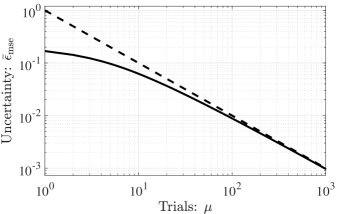
Figure 1: Mean square error optimised shot by shot (solid line) and quantum Cramér-Rao bound (dashed line) for the qubit network in Sec. III.1, with $\gamma=1$ and a prior area $\pi^{2}/4$ centred around $(0,0)$. This scheme is optimal at least for $\mu=1$ and $\mu\gg 1$. Note that $\bar{\epsilon}_{\mathrm{cr}}=1/\mu$ when $\gamma=1$ Proctor et al. (2017).

Let us start with the single-shot analysis. Assuming moderate prior knowledge given by $p(\theta_{1},\theta_{2})=4/\pi^{2}$ when $(\theta_{1},\theta_{2})\in[-\pi/4,\pi/4]\times[-\pi/4,\pi/4]$, and zero otherwise, the quantum estimators arising from $S_{i}\rho+\rho S_{i}=2\bar{\rho_{i}}$, $\rho=\int d\bm{\theta}p(\bm{\theta})\rho(\bm{\theta})$ and $\bar{\rho}_{i}=\int d\bm{\theta}p(\bm{\theta})\rho(\bm{\theta})\theta_{i}$ are

$$S_{1}=\frac{2\left(4-\pi\right)}{\pi\left(1+\gamma^{2}\right)}\left[\frac{\gamma}{\sqrt{2}}\sigma_{y}\otimes\mathbb{I}+\frac{1-\gamma^{2}}{\pi}\sigma_{x}\otimes\sigma_{y}\right],$$ (15)

$$S_{2}=\frac{2\left(4-\pi\right)}{\pi\left(1+\gamma^{2}\right)}\left[\frac{\gamma}{\sqrt{2}}\mathbb{I}\otimes\sigma_{y}+\frac{1-\gamma^{2}}{\pi}\sigma_{y}\otimes\sigma_{x}\right],$$ (16)

where the columns are labelled as $\ket{00}$, $\ket{01}$, $\ket{10}$ and $\ket{11}$, and $\sigma_{x}$ and $\sigma_{y}$ are Pauli matrices. In addition, the bound in Eq. (9) implies that

$$\bar{\epsilon}_{\mathrm{mse}}\geqslant\frac{\pi^{2}}{48}-\frac{2\left(4-\pi\right)^{2}\left[2-\left(4-\pi^{2}\right)\gamma^{2}+2\gamma^{4}\right]}{\pi^{4}\left(1+\gamma^{2}\right)^{2}}$$ (17)

for $\mu=1$, which achieves its minimum at $\gamma=\pm 1$. That is, $\bar{\epsilon}_{\mathrm{mse}}\geqslant\pi^{2}/48-(4-\pi)^{2}/(2\pi^{2})\approx 0.168$. Appendix C provides the details of these calculations.

Since $[S_{1},S_{2}]=0$, there is a measurement achieving the minimum single-shot error above. Choosing $\gamma=1$ we can construct an optimal strategy given by the projectors $\ket{s_{+},s_{+}}$, $\ket{s_{-},s_{-}}$, $\ket{s_{+},s_{-}}$, $\ket{s_{-},s_{+}}$, where $\ket{s_{\pm}}=(\ket{0}\pm i\ket{1})/\sqrt{2}$, and calculate the uncertainty for $\mu$ trials in Eq. (14) using this measurement in each shot. The solid line in Fig. 1 shows this numerical result, while the dashed line is the quantum Cramér-Rao bound. Given that the latter is approached by the Bayesian error as $\mu$ grows, we see that our Bayesian strategy is optimal both for $\mu=1$ and $\mu\gg 1$, in consistency with the behaviour observed in the single-parameter case Rubio and Dunningham (2019).

Additionally, note that the asymptotic theory is a good approximation to our bound (i.e., their relative error is less than $5\%$ Rubio et al. (2018); Rubio (2020)) only when $\mu>5.05\cdot 10^{2}$, while there exist practical multi-parameter schemes where, e.g., $\mu=3\cdot 10^{2}$ Berchera and Degiovanni (2019) and $\mu=10^{2}$ Polino et al. (2019). This demonstrates the potential relevance of our approach in experiments.

In fact, it can be shown that our optimisation of this protocol provides a meaningful amount of information even for a single shot. Indeed, by noticing that $\bar{\epsilon}_{\mathrm{prior}}=\pi^{2}/48\approx 0.206$, and defining a notion of improvement as $(\bar{\epsilon}_{\mathrm{prior}}-\bar{\epsilon}_{\mathrm{mse}})/\bar{\epsilon}_{\mathrm{prior}}$ multiplied by $100\%$, we see that a single shot improves our knowledge about $(\theta_{1},\theta_{2})$ by $18\%$ with respect to the prior uncertainty .

From a fundamental perspective, a remarkable conclusion of our analysis is that this qubit sensing network reaches its optimal single-shot error without entanglement, since the strategy above is local in the sense that both the state and the measurement are separable. In other words, we have shown that this result, which previously had been established only in an asymptotic fashion Proctor et al. (2017), is also valid for repeated experiments with limited data and moderate prior.

III.2 Quantum imaging

Secondly we wish to examine the phase imaging model explored in Humphreys et al. (2013); Knott et al. (2016) with the Cramér-Rao bound, and in Macchiavello (2003) using covariant measurements. In the former the scheme operates asymptotically, while the latter assumes no prior knowledge. On the contrary, our protocol will assume an intermediate amount of prior information.

Consider a system with $(d+1)$ optical modes where we encode a phase shift $\theta_{j}$ with a local unitary $U(\theta_{j})=\mathrm{exp}(-ia_{j}^{\dagger}a_{j}\theta_{j})$ in the $j$-th mode, for $1\leqslant j\leqslant d$, while $j=0$ is a reference mode calibrated in advance Proctor et al. (2017). Note that $a_{j}^{\dagger}$ and $a_{j}$ are creation and annihilation operators. Given this, one possibility is following a global approach and preparing the entangled probe Knott et al. (2016); Humphreys et al. (2013)

$$\ket{\psi_{0}}=\frac{1}{\sqrt{d+\alpha^{2}}}\left(\alpha\ket{\bar{n}_{0}}+\sum_{k=1}^{d}\ket{\bar{n}_{k}}\right),$$ (18)

where $\ket{\bar{n}_{j}}$ is a state with $\bar{n}$ photons in the $j$-th mode and zero in the rest, $\bar{n}$ is the mean number of quanta and $\alpha$ is assumed to be real. This is a generalised NOON state.

Suppose that the unknown parameters are equally important, so that $\mathcal{W}=\mathbb{I}/d$, and consider a flat prior of hypervolume $(2\pi/\bar{n})^{d}$ with $\bar{n}\geqslant 4$ and centred around $(0,0,\dots)$. This prior knowledge is sufficient to avoid the periodicities associated with NOON states and to employ the square error in phase estimation Rubio et al. (2018); Rubio and Dunningham (2019); Luis (2017); Hall and Wiseman (2012); Friis et al. (2017).

Our calculations in Appendix D show that, for this scheme,

$$S_{k}=\frac{-2i\alpha}{\bar{n}\left(1+\alpha^{2}\right)}\left(\outerproduct{\bar{n}_{k}}{\bar{n}_{0}}-\outerproduct{\bar{n}_{0}}{\bar{n}_{k}}\right)$$ (19)

after solving $S_{k}\rho+\rho S_{k}=2\bar{\rho_{k}}$, $\rho=\int d\bm{\theta}p(\bm{\theta})\rho(\bm{\theta})$ and $\bar{\rho}_{k}=\int d\bm{\theta}p(\bm{\theta})\rho(\bm{\theta})\theta_{k}$, and that Eq. (9) becomes

$$\bar{\epsilon}_{\mathrm{mse}}\geqslant\frac{1}{\bar{n}^{2}}\left[\frac{\pi^{2}}{3}-\frac{4\alpha^{2}}{\left(1+\alpha^{2}\right)\left(d+\alpha^{2}\right)}\right].$$ (20)

Since the latter achieves its minimum at $\alpha=d^{1/4}$,

$$\bar{\epsilon}_{\mathrm{mse}}\geqslant\frac{1}{\bar{n}^{2}}\left[\frac{\pi^{2}}{3}-\frac{4}{(1+\sqrt{d})^{2}}\right]\leavevmode\nobreak\ \underset{d\gg 1}{\longrightarrow}\leavevmode\nobreak\ \frac{1}{\bar{n}^{2}}\left(\frac{\pi^{2}}{3}-\frac{4}{d}\right)$$ (21)

is the single-shot bound for the global scheme.

Unlike in the qubit case, here $[S_{k},S_{j}]\neq 0$ when $k\neq j$, which means that we cannot extract an optimal measurement as we did before. However, the asymptotic theory has been shown to predict that the scaling associated with the state in Eq. (18) can also be achieved with a local scheme Knott et al. (2016). Therefore, if we could recover this phenomenon using our Bayesian bound, then we may be able to construct a single-shot strategy with a precision that scales as in Eq. (21).

In a local protocol we have that $\rho_{0}=\rho_{0}^{\mathrm{ref}}\otimes\rho_{0}^{(1)}\otimes\cdots\otimes\rho_{0}^{(d)}$, with $\rho_{0}^{(k)}=|\phi_{0}^{(k)}\rangle\langle\phi_{0}^{(k)}|$ for pure states. Following Knott et al. (2016) we choose $\ket{\phi_{0}}$ as

$$\ket{\phi_{0}}=\left[\sqrt{1-\frac{\bar{n}}{N(d+1)}}\ket{0}+\sqrt{\frac{\bar{n}}{N(d+1)}}\ket{N}\right],$$ (22)

where $N$ can vary while $\bar{n}$ remains constant. This is an important property, since it allows us to modify the precision through $N$ without altering the average amount of resources. More concretely, inserting the resulting state in Eq. (9) we find the bound (see Appendix D)

$$\bar{\epsilon}_{\mathrm{mse}}\geqslant\left[\pi^{2}/3-f(N,\bar{n},d)\right]/\bar{n}^{2},$$ (23)

where $f(N,\bar{n},d)$ satisfies that:

1. if $N=\bar{n}$, then $f(N,\bar{n},d)=4d/(1+d)^{2}$, and

   $$\bar{\epsilon}_{\mathrm{mse}}\geqslant\frac{1}{\bar{n}^{2}}\left[\frac{\pi^{2}}{3}-\frac{4d}{(1+d)^{2}}\right]\leavevmode\nobreak\ \leavevmode\nobreak\ \underset{d\gg 1}{\longrightarrow}\leavevmode\nobreak\ \leavevmode\nobreak\ \frac{1}{\bar{n}^{2}}\left(\frac{\pi^{2}}{3}-\frac{4}{d}\right);$$ (24)

2. if $N\rightarrow\infty$, then $f(N,\bar{n},d)\rightarrow 0$, so that

   $$\bar{\epsilon}_{\mathrm{mse}}\leavevmode\nobreak\ \leavevmode\nobreak\ \underset{N\rightarrow\infty}{\longrightarrow}\leavevmode\nobreak\ \leavevmode\nobreak\ \frac{\pi^{2}}{3\bar{n}^{2}}=\frac{1}{d}\sum_{i=1}^{d}\Delta\theta_{p,i}^{2}.$$ (25)

The scaling in Eq. (24) is exactly that found in Eq. (21) for the global strategy, and the bound associated with the local scheme can be reached. To see how, first note that if the parameters are a priori thought of as independent (a condition fulfilled by our separable prior), then $\rho=\rho_{0}^{\mathrm{ref}}\otimes\rho^{(1)}\otimes\cdots\otimes\rho^{(d)}$ and $\bar{\rho}_{k}=\rho_{0}^{\mathrm{ref}}\otimes\rho^{(1)}\otimes\cdots\otimes\bar{\rho}^{(k)}\otimes\cdots\otimes\rho^{(d)}$. In turn, $S_{k}=\mathbb{I}_{\mathrm{ref}}\otimes\mathbb{I}\otimes\cdots\otimes S^{(k)}\otimes\cdots\otimes\mathbb{I}$, so that $S_{k}$ commutes trivially with the rest. Hence, despite the non-commutative nature of the estimators associated with the original global protocol, we can still construct a strategy with the desired scaling by using local states and measurements, as we did with the qubit network.

The previous discussion also shows that, for protocols with moderate prior knowledge and limited measurement data, a global strategy is not required to achieve the scaling predicted in Eq. (21) . This is similar to our conclusion in Sec. III.1 for the qubit network, but the imaging protocol provides a more fundamental way of understanding the importance of this result.

First we recall that, according to the asymptotic theory, the precision of schemes such as Eq. (22) appears to grow unbounded as $N$ is increased Rivas and Luis (2012); Knott et al. (2016); Rubio et al. (2018); Tsang (2012); Lee et al. (2019), while a finite precision is known to be recovered when the prior information is appropriately taken into account Tsang (2012); Berry et al. (2012); Hall and Wiseman (2012); Rubio et al. (2018); Giovannetti and Maccone (2012); Pezzè (2013); Demkowicz-Dobrzański et al. (2015); Rubio (2020). This means that our local scheme will not be able to produce an arbitrarily good precision by simply increasing $N$, and this is precisely what Eq. (25) demonstrates. To understand it, note that the periodicity in Eq. (22) is $2\pi/N$, so that the width where the value of each phase may lie needs to be smaller as $N$ grows to avoid ambiguities, and thus the limit $N\rightarrow\infty$ is equivalent to requiring that the parameters are practically localised a priori. Since the prior knowledge is fixed by the situation under analysis, eventually the high amount of prior information needed as $N$ grows is not provided, and the scheme is unable to extract more information beyond our initial knowledge.

Therefore, if we were to restrict our calculations to the framework provided by the quantum Fisher information matrix and the associated Cramér-Rao bound, then one could question the physical validity of searching for local strategies that are as sensitive as a global scheme (see, e.g., Knott et al. (2016); Proctor et al. (2017, 2018); Altenburg and Wölk (2018)), for the apparent enhancement of the local approach might not be such. Our Bayesian analysis shows that this type of result can in fact emerge in a more realistic regime with finite resources and without involving unbounded precisions, and this puts the idea that some local schemes reproduce the enhancements predicted by certain global protocols on a solid basis.

IV Discussion and conclusions

Our method offers a powerful and novel framework to study schemes with limited data and moderate prior knowledge, a regime of practical interest and often outside of the scope of existing techniques. Given that experimental multi-parameter protocols are already a reality Roccia et al. (2018); Polino et al. (2019); Berchera and Degiovanni (2019); Valeri et al. (2020), our proposal could play a crucial role in the design of future experiments.

Theoretically, a major strength of our derivation of Eq. (9) is its clear separation of the classical optimisation from the quantum problem, in analogy with the proof of the Braunstein-Caves inequality Braunstein and Caves (1994); Genoni et al. (2008). One could be tempted to argue that by introducing $S_{u}\rho+\rho S_{u}=2\bar{\rho}_{u}$ we are somehow assuming the answer, as this is the solution of the single-parameter optimisation. However, here this equation is a redefinition of $\bar{\rho}_{u}$ allowing us to derive a bound, and its form is imposed by the formal analogy with the Fisher information. Moreover, given the scalar quantity $\bm{u}^{\mathchoice{\raisebox{0.0pt}{$\displaystyle\intercal$}}{\raisebox{0.0pt}{$\textstyle\intercal$}}{\raisebox{0.0pt}{$\scriptstyle\intercal$}}{\raisebox{0.0pt}{$\scriptscriptstyle\intercal$}}}\Sigma_{\mathrm{mse}}\bm{u}$, we could instead employ any of the alternative single-parameter proofs available Personick (1971); Helstrom (1976); Macieszczak et al. (2014) to show that $\bm{u}^{\mathchoice{\raisebox{0.0pt}{$\displaystyle\intercal$}}{\raisebox{0.0pt}{$\textstyle\intercal$}}{\raisebox{0.0pt}{$\scriptstyle\intercal$}}{\raisebox{0.0pt}{$\scriptscriptstyle\intercal$}}}\Sigma_{\mathrm{mse}}\bm{u}\geqslant\int d\bm{\theta}p(\bm{\theta})\theta_{u}^{2}-\mathrm{Tr}(\rho S_{u}^{2})$, from where (9) follows, although these approaches, unlike ours, merge classical and quantum steps.

Among all the Bayesian bounds neglecting the interference between individually optimal quantum strategies, our result is to be preferred, since it recovers the true optimum both in the single-parameter limit and when $\{S_{i}\}$ commute. Moreover, our qubit and optical examples demonstrate that its calculation can be tractable, and that the Bayesian nature of our approach can produce a more physical picture of the performance associated with multi-parameter protocols. Additionally, note that while Eq. (9) may not always produce tight bounds, we can still use it to study how close a given measurement can get (see Appendix E for an example of this type of calculation). Hence, this tool will be very useful to enquire about fundamental limits or the precision scaling in a range of practical cases.

Finally, our approach could be key to finding fundamental bounds including the case of non-commuting estimators. In particular, the rationale behind our Bayesian analogue of the Helstrom Cramér-Rao bound might also lead us to a similar Bayesian analogue of the Holevo Cramér-Rao bound , which could eliminate the deficiencies of both our result and the standard Holevo Cramér-Rao bound and move us closer to the optima predicted by Holevo and Helstrom’s often intractable fundamental equations Helstrom (1976); Helstrom and Kennedy (1974); Holevo (1973a, b); Rubio (2020). This path promises a bright future for multi-parameter metrology.

Appendix A Optimal classical estimators

The form of the optimal classical estimators for the multi-parameter square error is a well-known result Kay (1993). To recover it as the matrix inequality $\Sigma_{\mathrm{mse}}\geqslant\Sigma_{c}$, first we note that the variational problem

$$\delta\epsilon\left[g_{u}(m)\right]=\delta\int dm\leavevmode\nobreak\ \mathcal{L}\left[m,g_{u}(m)\right]=0,$$ (26)

with $\mathcal{L}\left[m,g_{u}(m)\right]=\int d\bm{\theta}p(\bm{\theta},m)\left[g_{u}(m)-\theta_{u}\right]^{2}$ and $x_{u}=\sum_{i=1}^{d}u_{i}x_{i}$, is equivalent to require that Riley et al. (2004)

$$\frac{d}{d\beta}\epsilon\left[g_{u}(m)+\beta h_{u}(m)\right]\bigg{\rvert}_{\beta=0}=0,\leavevmode\nobreak\ \leavevmode\nobreak\ \text{for\leavevmode\nobreak\ all}\leavevmode\nobreak\ \leavevmode\nobreak\ h_{u}(m).$$ (27)

In our case we have that

$$\frac{d}{d\beta} \epsilon\left[g_{u}(m)+\beta h(m)\right]$$ (28)

$$=2\int d\bm{\theta}dm\leavevmode\nobreak\ p(\bm{\theta},m)\left[g_{u}(m)+\beta h_{u}(m)-\theta_{u}\right]h_{u}(m),$$

which means that the requirement to find the extrema is

$$\frac{d}{d\beta} \epsilon\left[g_{u}(m)+\beta h_{u}(m)\right]\bigg{\rvert}_{\beta=0}$$

$$=2\int d\bm{\theta}dm\leavevmode\nobreak\ p(\bm{\theta},m)\left[g_{u}(m)-\theta_{u}\right]h_{u}(m)=0,$$ (29)

and this implies that $\int d\bm{\theta}p(\bm{\theta},m)[g_{u}(m)-\theta_{u}]=0$ if Eq. (29) is to be satisfied by an arbitrary $h_{u}(m)$. By decomposing the joint probability as $p(\bm{\theta},m)=p(m)p(\bm{\theta}|m)$, with $p(\bm{\theta}|m)\propto p(\bm{\theta})p(m|\bm{\theta})$, we see that the solution

$$g_{u}(m)=\int d\bm{\theta}p(\bm{\theta}|m)\theta_{u}$$ (30)

makes the error $\epsilon\left[g_{u}(m)\right]$ extremal.

To verify that this is a minimum we can use the functional version of the second derivative test. Calculating the second variation from Eq. (28) we see that

$$\frac{d^{2}}{d\beta^{2}} \epsilon\left[g_{u}(m)+\beta h_{u}(m)\right]\bigg{\rvert}_{\beta=0}$$

$$=2\int d\bm{\theta}dm\leavevmode\nobreak\ p(\bm{\theta},m)h_{u}(m)^{2}>0$$ (31)

for non-trivial variations. Thus $g_{u}(m)=\int d\theta p(\bm{\theta}|m)\theta_{u}$ gives the minimum of $\epsilon\left[g_{u}(m)\right]=\bm{u}^{\mathchoice{\raisebox{0.0pt}{$\displaystyle\intercal$}}{\raisebox{0.0pt}{$\textstyle\intercal$}}{\raisebox{0.0pt}{$\scriptstyle\intercal$}}{\raisebox{0.0pt}{$\scriptscriptstyle\intercal$}}}\Sigma_{\mathrm{mse}}\bm{u}$, and

$$\bm{u}^{\mathchoice{\raisebox{0.0pt}{$\displaystyle\intercal$}}{\raisebox{0.0pt}{$\textstyle\intercal$}}{\raisebox{0.0pt}{$\scriptstyle\intercal$}}{\raisebox{0.0pt}{$\scriptscriptstyle\intercal$}}}\Sigma_{\mathrm{mse}}\bm{u} \geqslant\int d\bm{\theta}p(\bm{\theta})\theta_{u}^{2}-\int dm\frac{\left[\int d\bm{\theta}p(\bm{\theta})p(m|\bm{\theta})\theta_{u}\right]^{2}}{\int d\bm{\theta}p(\bm{\theta})p(m|\bm{\theta})}$$

$$=\bm{u}^{\mathchoice{\raisebox{0.0pt}{$\displaystyle\intercal$}}{\raisebox{0.0pt}{$\textstyle\intercal$}}{\raisebox{0.0pt}{$\scriptstyle\intercal$}}{\raisebox{0.0pt}{$\scriptscriptstyle\intercal$}}}\Sigma_{c}\bm{u}$$ (32)

for any $\bm{u}$, where $\Sigma_{c}$ is the optimal matrix error

$$\Sigma_{c}= \int d\bm{\theta}p(\bm{\theta})\bm{\theta}\bm{\theta}^{\mathchoice{\raisebox{0.0pt}{$\displaystyle\intercal$}}{\raisebox{0.0pt}{$\textstyle\intercal$}}{\raisebox{0.0pt}{$\scriptstyle\intercal$}}{\raisebox{0.0pt}{$\scriptscriptstyle\intercal$}}}$$ (33)

$$-\int dm\frac{\left[\int d\bm{\theta}p(\bm{\theta})p(m|\bm{\theta})\bm{\theta}\right]\left[\int d\bm{\theta}p(\bm{\theta})p(m|\bm{\theta})\bm{\theta}\right]^{\mathchoice{\raisebox{0.0pt}{$\displaystyle\intercal$}}{\raisebox{0.0pt}{$\textstyle\intercal$}}{\raisebox{0.0pt}{$\scriptstyle\intercal$}}{\raisebox{0.0pt}{$\scriptscriptstyle\intercal$}}}}{\int d\bm{\theta}p(\bm{\theta})p(m|\bm{\theta})}.$$

In this way we have arrived at the desired matrix inequality, i.e., $\Sigma_{\mathrm{mse}}\geqslant\Sigma_{c}$.

Appendix B Matrix form of $\mathcal{K}_{u}$

A crucial step to find the quantum inequality $\Sigma_{c}\geqslant\Sigma_{q}$ that constitutes one of our main results is to rewrite $\mathcal{K}_{u}=\mathrm{Tr}(\rho S_{u}^{2})$ as $\mathcal{K}_{u}=\bm{u}^{\mathchoice{\raisebox{0.0pt}{$\displaystyle\intercal$}}{\raisebox{0.0pt}{$\textstyle\intercal$}}{\raisebox{0.0pt}{$\scriptstyle\intercal$}}{\raisebox{0.0pt}{$\scriptscriptstyle\intercal$}}}\mathcal{K}\bm{u}$, where $\mathcal{K}_{ij}=\mathrm{Tr}(\rho A_{ij})$ is a matrix and $A_{ij}$ is some operator associated with the product of $S_{i}$ and $S_{j}$. Since $S_{i}$ and $S_{j}$ might not commute, in principle we could consider either $A_{ij}=S_{i}S_{j}$, $A_{ij}=S_{j}S_{i}$ or $A_{ij}=(S_{i}S_{j}+S_{j}S_{i})/2$. However, if we first decompose $A_{ij}$ as $2A_{ij}=(A_{ij}+A_{ij}^{\dagger})+(A_{ij}-A_{ij}^{\dagger})$, so that

$$\bm{u}^{\mathchoice{\raisebox{0.0pt}{$\displaystyle\intercal$}}{\raisebox{0.0pt}{$\textstyle\intercal$}}{\raisebox{0.0pt}{$\scriptstyle\intercal$}}{\raisebox{0.0pt}{$\scriptscriptstyle\intercal$}}}\mathcal{K}\bm{u}=\frac{1}{2}\left(\sum_{i,j=1}^{d}u_{i}u_{j}C^{+}+\sum_{i,j=1}^{d}u_{i}u_{j}C^{-}\right),$$ (34)

with $C^{\pm}=\mathrm{Tr}[\rho(A_{ij}\pm A_{ij}^{\dagger})]$, and observing that $\bm{u}$ is real and $S_{i}$ Hermitian, then

$$\bm{u}^{\mathchoice{\raisebox{0.0pt}{$\displaystyle\intercal$}}{\raisebox{0.0pt}{$\textstyle\intercal$}}{\raisebox{0.0pt}{$\scriptstyle\intercal$}}{\raisebox{0.0pt}{$\scriptscriptstyle\intercal$}}}\mathcal{K}\bm{u} =\frac{1}{2}\sum_{i,j=1}^{d}u_{i}u_{j}\mathrm{Tr}\left[\rho\left(S_{i}S_{j}+S_{j}S_{i}\right)\right]$$

$$=\mathrm{Tr}\left(\rho S_{u}^{2}\right)=\mathcal{K}_{u}$$ (35)

for any of the three possible forms of $A_{ij}$. Therefore, we can take $\mathcal{K}$ to be a symmetric matrix with elements

$$\mathcal{K}_{ij}=\mathrm{Tr}\left[\rho\left(S_{i}S_{j}+S_{j}S_{i}\right)\right]/2.$$ (36)

See Helstrom (1968) for the analogous step in the derivation of the multi-parameter quantum Cramér-Rao bound.

Appendix C Calculations for the qubit network

Given the network state

$$\ket{\psi_{0}}=\frac{1}{\sqrt{2(1+\gamma^{2})}}\left[\ket{00}+\gamma(\ket{01}+\ket{10})+\ket{11}\right],$$ (37)

the unitary encoding

$$U(\theta_{1},\theta_{2})=\mathrm{exp}\left[-i\left(\sigma_{z,1}\theta_{1}+\sigma_{z,2}\theta_{2}\right)/2\right],$$ (38)

and the prior density $p(\theta_{1},\theta_{2})=4/\pi^{2}$, when $(\theta_{1},\theta_{2})\in[-\pi/4,\pi/4]\times[-\pi/4,\pi/4]$, we have that

$$\rho =\int d\theta_{1}d\theta_{2}p(\theta_{1},\theta_{2})\rho(\theta_{1},\theta_{2})$$

$$=\frac{4}{\pi^{2}}\int_{-\pi/4}^{\pi/4}d\theta_{1}\int_{-\pi/4}^{\pi/4}d\theta_{2}\hskip 1.49994ptU(\theta_{1},\theta_{2})\outerproduct{\psi_{0}}{\psi_{0}}U^{\dagger}(\theta_{1},\theta_{2})$$

$$=\frac{1}{2\pi^{2}(1+\gamma^{2})}\left(\begin{array}[]{cccc}\pi^{2}&2\sqrt{2}\pi\gamma&2\sqrt{2}\pi\gamma&8\\ 2\sqrt{2}\pi\gamma&\pi^{2}\gamma^{2}&8\gamma^{2}&2\sqrt{2}\pi\gamma\\ 2\sqrt{2}\pi\gamma&8\gamma^{2}&\pi^{2}\gamma^{2}&2\sqrt{2}\pi\gamma\\ 8&2\sqrt{2}\pi\gamma&2\sqrt{2}\pi\gamma&\pi^{2}\\ \end{array}\right),$$ (43)

$$\bar{\rho}_{1} =\int d\theta_{1}d\theta_{2}p(\theta_{1},\theta_{2})\rho(\theta_{1},\theta_{2})\theta_{1}$$

$$=\frac{4}{\pi^{2}}\int_{-\pi/4}^{\pi/4}d\theta_{1}\int_{-\pi/4}^{\pi/4}d\theta_{2}\hskip 1.49994ptU(\theta_{1},\theta_{2})\outerproduct{\psi_{0}}{\psi_{0}}U^{\dagger}(\theta_{1},\theta_{2})\theta_{1}$$

$$=\frac{i(4-\pi)}{2\sqrt{2}\pi^{2}(1+\gamma^{2})}\begin{pmatrix}0&0&-\pi\gamma&-2\sqrt{2}\\ 0&0&-2\sqrt{2}\gamma^{2}&-\pi\gamma\\ \pi\gamma&2\sqrt{2}\gamma^{2}&0&0\\ 2\sqrt{2}&\pi\gamma&0&0\end{pmatrix},$$ (44)

and

$$\bar{\rho}_{2} =\int d\theta_{1}d\theta_{2}p(\theta_{1},\theta_{2})\rho(\theta_{1},\theta_{2})\theta_{2}$$

$$=\frac{4}{\pi^{2}}\int_{-\pi/4}^{\pi/4}d\theta_{1}\int_{-\pi/4}^{\pi/4}d\theta_{2}\hskip 1.49994ptU(\theta_{1},\theta_{2})\outerproduct{\psi_{0}}{\psi_{0}}U^{\dagger}(\theta_{1},\theta_{2})\theta_{2}$$

$$=\frac{i(4-\pi)}{2\sqrt{2}\pi^{2}(1+\gamma^{2})}\begin{pmatrix}0&-\pi\gamma&0&-2\sqrt{2}\\ \pi\gamma&0&2\sqrt{2}\gamma^{2}&0\\ 0&-2\sqrt{2}\gamma^{2}&0&-\pi\gamma\\ 2\sqrt{2}&0&\pi\gamma&0\end{pmatrix},$$ (45)

where the columns are labelled as $\ket{00}$, $\ket{01}$, $\ket{10}$ and $\ket{11}$. In addition, by inserting Eqs. (43 - 45) in $S_{i}\rho+\rho S_{i}=2\bar{\rho}_{i}$ and using a computing system such as Mathematica to solve this Sylvester equation, we find that

$$S_{1} =\frac{2\left(4-\pi\right)}{\pi\left(1+\gamma^{2}\right)}\left(\frac{\gamma}{\sqrt{2}}\sigma_{y}\otimes\mathbb{I}+\frac{1-\gamma^{2}}{\pi}\sigma_{x}\otimes\sigma_{y}\right),$$

$$S_{2} =\frac{2\left(4-\pi\right)}{\pi\left(1+\gamma^{2}\right)}\left(\frac{\gamma}{\sqrt{2}}\mathbb{I}\otimes\sigma_{y}+\frac{1-\gamma^{2}}{\pi}\sigma_{y}\otimes\sigma_{x}\right),$$ (46)

where we have expressed the quantum estimators in terms of Pauli matrices to better visualise their structure. Introducing now Eq. (43) and Eq. (46) in the single-shot bound derived in this work we find that

$$\bar{\epsilon}_{\mathrm{mse}} \geqslant\sum_{i=1}^{2}w_{i}\left[\int d\theta_{1}d\theta_{2}p(\theta_{1},\theta_{2})\theta_{i}^{2}-\mathrm{Tr}\left(\rho S_{i}^{2}\right)\right]$$

$$=\frac{1}{2}\sum_{i=1}^{2}\left[\frac{4}{\pi^{2}}\int_{-\pi/4}^{\pi/4}d\theta_{1}\int_{-\pi/4}^{\pi/4}d\theta_{2}\hskip 1.49994pt\theta_{i}^{2}-\mathrm{Tr}\left(\rho S_{i}^{2}\right)\right]$$

$$=\frac{\pi^{2}}{48}-\frac{2\left(4-\pi\right)^{2}\left[2-\left(4-\pi^{2}\right)\gamma^{2}+2\gamma^{4}\right]}{\pi^{4}\left(1+\gamma^{2}\right)^{2}},$$ (47)

which is the error for $\mu=1$ examined in the main text.

On the other hand, if we choose $\gamma=1$, which is one of the values that gives the minimum single-shot error, then the quantum estimators in Eq. (46) become

$$S_{1}=\frac{\left(4-\pi\right)}{\pi\sqrt{2}}\sigma_{y}\otimes\mathbb{I},\leavevmode\nobreak\ \leavevmode\nobreak\ S_{2}=\frac{\left(4-\pi\right)}{\pi\sqrt{2}}\mathbb{I}\otimes\sigma_{y}.$$ (48)

It is thus clear that the tensor products of the eigenvectors of $\sigma_{y}$ form a common set of eigenvectors. This is how we arrive at the strategy in the main text given by the projectors $\ket{s_{+},s_{+}}$, $\ket{s_{-},s_{-}}$, $\ket{s_{+},s_{-}}$, $\ket{s_{-},s_{+}}$, with $\ket{s_{\pm}}=(\ket{0}\pm i\ket{1})/\sqrt{2}$.

Appendix D Calculations for phase imaging

In this work we have considered a quantum imaging protocol based on the unitary Macchiavello (2003); Humphreys et al. (2013); Knott et al. (2016)

$$U(\bm{\theta}) =\mathrm{exp}\left(-i\sum_{k=1}^{d}a_{k}^{\dagger}a_{k}\theta_{k}\right)=\mathrm{exp}\left(-i\sum_{k=1}^{d}N_{k}\theta_{k}\right)$$

$$\equiv\mathrm{exp}\left(-i\bm{N}\cdot\bm{\theta}\right),$$ (49)

and we have assumed a flat prior with hypervolume $(2\pi/\bar{n})^{d}$ and centre $\bar{\theta}=(0,0,\dots)$. For the global strategy

$$\ket{\psi_{0}}=\frac{1}{\sqrt{d+\alpha^{2}}}\left(\alpha\ket{\bar{n}_{0}}+\sum_{k=1}^{d}\ket{\bar{n}_{k}}\right),$$ (50)

where $\ket{\bar{n}_{j}}\equiv\ket{0}_{0}\otimes\cdots\otimes\ket{0}_{j-1}\otimes\ket{\bar{n}}_{j}\otimes\ket{0}_{j+1}\otimes\cdots\ket{0}_{d}=\ket{0\dots 0\leavevmode\nobreak\ \bar{n}\leavevmode\nobreak\ 0\dots 0}$, we have that

$$\rho =\left(\frac{\bar{n}}{2\pi}\right)^{d}\int_{-\pi/\bar{n}}^{\pi/\bar{n}}d\theta_{1}\cdots\int_{-\pi/\bar{n}}^{\pi/\bar{n}}d\theta_{d}\hskip 1.49994pt\mathrm{e}^{-i\bm{N}\cdot\bm{\theta}}\outerproduct{\psi_{0}}{\psi_{0}}\mathrm{e}^{i\bm{N}\cdot\bm{\theta}}$$

$$=\frac{1}{d+\alpha^{2}}\left(\alpha^{2}\outerproduct{\bar{n}_{0}}{\bar{n}_{0}}+\sum_{k=1}^{d}\outerproduct{\bar{n}_{k}}{\bar{n}_{k}}\right),$$ (51)

and that

$$\bar{\rho}_{k} =\left(\frac{\bar{n}}{2\pi}\right)^{d}\int_{-\pi/\bar{n}}^{\pi/\bar{n}}d\theta_{1}\cdots\int_{-\pi/\bar{n}}^{\pi/\bar{n}}d\theta_{d}\hskip 1.49994pt\mathrm{e}^{-i\bm{N}\cdot\bm{\theta}}\outerproduct{\psi_{0}}{\psi_{0}}\mathrm{e}^{i\bm{N}\cdot\bm{\theta}}\theta_{k}$$

$$=\frac{-i\alpha}{\bar{n}\left(d+\alpha^{2}\right)}\left(\outerproduct{\bar{n}_{k}}{\bar{n}_{0}}-\outerproduct{\bar{n}_{0}}{\bar{n}_{k}}\right),$$ (52)

having used the fact that

$$\int_{-\pi/\bar{n}}^{\pi/\bar{n}}d\theta_{j}=\frac{2\pi}{\bar{n}},$$

$$\int_{-\pi/\bar{n}}^{\pi/\bar{n}}d\theta_{j}\hskip 1.49994pt\theta_{j}=\int_{-\pi/\bar{n}}^{\pi/\bar{n}}d\theta_{j}\hskip 1.49994pt\mathrm{e}^{\pm i\bar{n}\theta_{j}}=0,$$

$$\int_{-\pi/\bar{n}}^{\pi/\bar{n}}d\theta_{j}\hskip 1.49994pt\mathrm{e}^{\pm i\bar{n}\theta_{j}}\theta_{j}=\pm\frac{2i\pi}{\bar{n}^{2}}.$$ (53)

Next we need to solve $S_{k}\rho+\rho S_{k}=2\bar{\rho_{k}}$. If we decompose $\rho$ in Eq. (43) as $\rho=\sum_{i}p_{i}\outerproduct{\phi_{i}}{\phi_{i}}$ and insert it in $S_{i}\rho+\rho S_{i}=2\bar{\rho}_{i}$, then we can rewrite $S_{i}$ as Rubio and Dunningham (2019)

$$S_{k}=2\sum_{j,l}\frac{\bra{\phi_{j}}\bar{\rho_{k}}\ket{\phi_{l}}}{p_{j}+p_{l}}\outerproduct{\phi_{j}}{\phi_{l}}.$$ (54)

By observing that $\rho$ in Eq. (51) is already diagonal, Eq. (54) simply becomes

$$S_{k}=\frac{-2i\alpha}{\bar{n}\left(1+\alpha^{2}\right)}\left(\outerproduct{\bar{n}_{k}}{\bar{n}_{0}}-\outerproduct{\bar{n}_{0}}{\bar{n}_{k}}\right)$$ (55)

after using Eq. (52).

The results for $\rho$ and $S_{k}$ can be now inserted in our single-shot bound, recovering in this way the bound in the main text, that is,

$$\bar{\epsilon}_{\mathrm{mse}} \geqslant\sum_{k=1}^{d}w_{k}\left[\int d\bm{\theta}p(\bm{\theta})\theta_{k}^{2}-\mathrm{Tr}\left(\rho S_{k}^{2}\right)\right]$$

$$=\frac{1}{d}\sum_{k=1}^{d}\left[\left(\frac{\bar{n}}{2\pi}\right)^{d}\int_{-\pi/\bar{n}}^{\pi/\bar{n}}d\theta_{1}\cdots\int_{-\pi/\bar{n}}^{\pi/\bar{n}}d\theta_{d}\hskip 1.49994pt\theta_{i}^{2}-\mathrm{Tr}\left(\rho S_{k}^{2}\right)\right]$$

$$=\frac{1}{\bar{n}^{2}}\left[\frac{\pi^{2}}{3}-\frac{4\alpha^{2}}{\left(1+\alpha^{2}\right)\left(d+\alpha^{2}\right)}\right].$$ (56)

Regarding the local strategy $\rho_{0}=\rho_{0}^{\mathrm{ref}}\otimes\rho_{0}^{(1)}\otimes\cdots\otimes\rho_{0}^{(d)}$, with $\rho_{0}^{(k)}=|\phi_{0}^{(k)}\rangle\langle\phi_{0}^{(k)}|$ and

$$|\phi_{0}^{(k)}\rangle=\left[\sqrt{1-\frac{\bar{n}}{N(d+1)}}\ket{0}+\sqrt{\frac{\bar{n}}{N(d+1)}}\ket{N}\right]\equiv\ket{\phi_{0}},$$ (57)

the single-shot bound can be written as

$$\bar{\epsilon}_{\mathrm{mse}} \geqslant\frac{1}{d}\sum_{k=1}^{d}\left[\left(\frac{\bar{n}}{2\pi}\right)^{d}\int_{-\pi/\bar{n}}^{\pi/\bar{n}}d\theta_{1}\cdots\int_{-\pi/\bar{n}}^{\pi/\bar{n}}d\theta_{d}\hskip 1.49994pt\theta_{i}^{2}-\mathrm{Tr}\left(\rho S_{k}^{2}\right)\right]$$

$$\equiv\frac{1}{\bar{n}^{2}}\left[\frac{\pi^{2}}{3}-f\left(N,\bar{n},d\right)\right].$$ (58)

Since the prior that we are using is separable, in this case we have that

$$\rho =\rho_{0}^{\mathrm{ref}}\otimes\rho^{(1)}\otimes\cdots\otimes\rho^{(d)},$$

$$\bar{\rho}_{k} =\rho_{0}^{\mathrm{ref}}\otimes\rho^{(1)}\otimes\cdots\otimes\bar{\rho}^{(k)}\otimes\cdots\otimes\rho^{(d)},$$

$$S_{k} =\mathbb{I}_{\mathrm{ref}}\otimes\mathbb{I}\otimes\cdots\otimes S^{(k)}\otimes\cdots\otimes\mathbb{I},$$ (59)

where the single-mode operators $\rho^{(k)}$, $\bar{\rho}^{(k)}$ and $S^{(k)}$ are identical for all the modes, and the calculation of the optimal single-shot uncertainty for the local estimation of several phases is effectively reduced to the single-parameter calculation

$$f\left(N,\bar{n},d\right)=\frac{\bar{n}^{2}}{d}\sum_{k=1}^{d}\mathrm{Tr}\left(\rho S_{k}^{2}\right)=\bar{n}^{2}\hskip 1.49994pt\mathrm{Tr}\left(\varrho S^{2}\right),$$ (60)

where $\rho^{(k)}\equiv\varrho$ and $S^{(k)}\equiv S$. Performing calculations analogous to those in previous examples (and similar to those in Rubio and Dunningham (2019) for single-parameter NOON states), we find

$$\varrho =\frac{1}{\pi N\left(1+\nu^{2}\right)}\begin{pmatrix}\nu^{2}\pi N&\bar{n}\nu\hskip 1.49994pt\mathrm{sin}\left(N\pi/\bar{n}\right)\\ \bar{n}\nu\hskip 1.49994pt\mathrm{sin}\left(N\pi/\bar{n}\right)&\pi N\end{pmatrix},$$

$$S =\frac{2\nu\left[N\pi\hskip 1.49994pt\mathrm{cos}\left(N\pi/\bar{n}\right)-\bar{n}\hskip 1.49994pt\mathrm{sin}\left(N\pi/\bar{n}\right)\right]}{\pi N^{2}\left(1+\nu^{2}\right)}\begin{pmatrix}0&-i\\ i&0\end{pmatrix}$$ (61)

for the state in Eq. (57), where $\nu=\sqrt{N(d+1)/\bar{n}-1}$. Therefore, Eq. (60) implies that

$$f\left(N,\bar{n},d\right)=\frac{4\bar{n}^{3}\left[\left(1+d\right)N-\bar{n}\right]a\left(N,\bar{n}\right)^{2}}{\pi^{2}N^{6}\left(1+d\right)^{2}},$$ (62)

where $a\left(N,\bar{n}\right)=N\pi\hskip 1.49994pt\mathrm{cos}\left(N\pi/\bar{n}\right)-\bar{n}\hskip 1.49994pt\mathrm{sin}\left(N\pi/\bar{n}\right)$, and as we mentioned in the main discussion, $f(N=\bar{n},\bar{n},d)=4d/(1+d)^{2}$ and $f(N\gg 1,\bar{n},d)\approx 0$.

Appendix E Performance of a phase imaging measurement versus our quantum bound

Consider the global phase imaging scheme in Eq. (49) and Eq. (50), and let us calculate the single-shot bound for $d=2$, $\bar{n}=2$, $\mathcal{W}=\mathbb{I}/2$, the same two-parameter prior probability that we employed in the qubit case, and $\alpha=1$, where the latter is the balanced version of Eq. (50) Knott et al. (2016). With this configuration we find that

$$\rho =\frac{1}{3}\left[\mathbb{I}+\frac{2(\lambda_{1}+\lambda_{4})}{\pi}+\frac{4\lambda_{6}}{\pi^{2}}\right],$$

$$\bar{\rho}_{1} =\frac{1}{3\pi}\left(\frac{2\lambda_{7}}{\pi}-\lambda_{2}\right),$$

$$\bar{\rho}_{2} =-\frac{1}{3\pi}\left(\frac{2\lambda_{7}}{\pi}+\lambda_{5}\right),$$ (63)

where $\lambda_{i}$ are Gell-Mann matrices Gell-Mann (1962). Furthermore, introducing these results in $S_{i}\rho+\rho S_{i}=2\bar{\rho}_{i}$ we find that the quantum estimators are

$$S_{1} =\frac{1}{\pi}\left[\frac{\lambda_{5}-(1+\pi^{2})\lambda_{2}}{2+\pi^{2}}+\frac{\lambda_{7}}{\pi}\right],$$

$$S_{2} =\frac{1}{\pi}\left[\frac{\lambda_{2}-(1+\pi^{2})\lambda_{5}}{2+\pi^{2}}-\frac{\lambda_{7}}{\pi}\right],$$ (64)

and the single-shot error is bounded as

$$\bar{\epsilon}_{\mathrm{mse}}\geqslant\frac{\pi^{2}}{48}-\frac{2\left(4+3\pi^{2}+\pi^{4}\right)}{3\pi^{4}\left(2+\pi^{2}\right)}\approx 0.130.$$ (65)

While we cannot extract an optimal measurement from $S_{1}$ and $S_{2}$ because $[S_{1},S_{2}]\neq 0$, a numerical search by trial and error has revealed an approximate set of projectors with a precision almost as good as that given in Eq. (65). In particular, if we use

$$\bra{\varphi_{a}} = (0.485+0.131i,0.441-0.070i,-0.223+0.706i),$$

$$\bra{\varphi_{b}} = (0.688,-0.208-0.432i,-0.270-0.472i),$$

$$\bra{\varphi_{c}} = (0.509+0.118i,-0.284+0.700i,0.396),$$ (66)

with components labelled as $\ket{2,0,0}$, $\ket{0,2,0}$, $\ket{0,0,2}$, and we employ the multi-parameter numerical algorithm in Rubio (2020), then we find that, for $\mu=1$, $\bar{\epsilon}_{\mathrm{mse}}\approx 0.142$.

Remarkably, this result suggests that, at least in this particular case, our multi-parameter bound is providing most of the information associated with the quantum part of the problem. Whether this is also the case in other configurations should be object of some future and highly interesting work.