CUR Low Rank Approximation of a Matrix at Sublinear Cost

Abstract

Low rank approximation of a matrix (hereafter LRA) is a highly important area of Numerical Linear and Multilinear Algebra and Data Mining and Analysis. One can operate with LRA at sublinear cost, that is, by using much fewer memory cells and flops than an input matrix has entries, but no sublinear cost algorithm can compute accurate LRA of the worst case input matrices or even of the matrices of small families in our Appendix A. Nevertheless we prove that Cross-Approximation (C-A) celebrated iterations and even more primitive sublinear cost algorithms output quite accurate LRA for a large subclass of the class of all matrices that admit sufficiently close LRA and in a sense for most of such matrices. Moreover, we accentuate the power of sublinear cost LRA by means of multiplicative pre-processing of an input matrix, and also compare C-A iterations with ADI-based variant of Randomized and Sketching LRA algorithms. Our tests are in good accordance with our formal study.

Key Words:

Low-rank approximation (LRA), CUR LRA, Sublinear cost, Cross-Approximation iterations

2020 Math. Subject Classification:

65Y20, 65F55, 68Q25, 68W20

1 Introduction

1.1. LRA at sublinear cost: the problem and background. LRA of a matrix is one of the most fundamental problems of Numerical Linear and Multilinear Algebra and Data Mining and Analysis, with applications ranging from machine learning theory and neural networks to term document data and DNA SNP data (see surveys [24, 29, 25]).

Matrices representing Big Data (e.g., unfolding matrices of multidimensional tensors) are usually so immense that realistically one can only access a tiny fraction of their entries, but quite typically these matrices admit LRA, that is, are close to low rank matrices, with which one can operate at sublinear cost.

Every LRA algorithm running at sublinear cost fails on the worst case inputs and even on the small families of the matrices of our Appendix A, but two decades ago some authors have ignored this information and proposed Cross-Approximation (C-A) iterations (the concept has been coined by E.E. Tyrtyshnikov in [48]). Since then these iterations have been routinely applied worldwide in computational practice and have been consistently computing accurate LRA of a large and important class of matrices at sublinear cost (see [47, 22, 23, 21, 48, 1, 19, 5, 4, 18, 20, 34, 33]).

1.2. Recent and new progress. The papers [38, 39, 34, 33] provide some formal support for such empirical observations. By extending that work we prove that C-A algorithms and even some more rudimentary algorithms, said to be Primitive and also running at sublinear cost, compute quite accurate LRA for a large subclass of the class of all matrices that admit their sufficiently close LRA, and in some sense for most of such matrices.

Namely, we define a large class of random matrices, which we call perturbed factor-Gaussian and which admit LRA, and prove that the C-A and Primitive algorithms whp compute close LRA of a random matrix of this class (see Sec. 6) or, as we say, compute the dual LRA for the matrices of this class.

All these sublinear cost algorithms output LRA in its special form of CUR LRA, traced back to [47, 22, 23, 21] and particularly memory efficient. In [37] we transform any LRA into CUR LRA at sublinear cost.

Our present study extends our earlier solution of some dual problems of matrix computations, in particular Gaussian elimination without pivoting, which is a communication costly stage (see [42, 44, 45]). This work has been further advanced in [41, 40, 27, 37, 28] and should motivate research effort towards the design and analysis of sublinear cost dual algorithms for LRA and other matrix computations.

1.3. Three limitations of our progress.

(a) Any model of randomization of LRA is odd to some important input classes encountered in computational practice, and our models are no exception,

(b) Our theorems only hold where an input matrix is sufficiently close to matrices of low rank (see our specific estimates in Lemma 5.3).

(c) The expected error norms of our LRA are within some specified factors from optimal (see our estimates in Section 6) but are not arbitrarily close to optimal (not relative error LRA).

1.4. Can we counter or alleviate these limitations?

In spite of these limitations our work can be of some interest from qualitative point of view; moreover our present study shows that the above problems are less severe than they may seem to be.

(a) Our tests with both synthetic and real world inputs are in good accordance with our formal study and even suggest that some of our formal error estimates are overly pessimistic in the case of C-A algorithms.

(b) Our dual solution of LRA can be extended at sublinear cost to randomized computation of LRA, which is accurate whp for any matrix that admits its LRA and is pre-processed by means of its multiplication by random Gaussian, SRFT, SRHT, or Rademacher’s matrices.

In particular we readily prove that pre-processing with random Gaussian multipliers turns any matrix that admits close LRA into a small norm perturbation of a factor-Gaussian matrix, for which we proved accuracy of LRA computed by the C-A iterations and Primitive algorithms. Pre-processing with these multipliers has superlinear cost, but in our tests pre-processing at sublinear cost with various sparse multipliers has consistently worked as efficiently.

Besides showing practical promise of LRA with pre-processing, our study reveals the relationship, so far unnoticed, between modified C-A iterations and Randomized and Sketching LRA algorithms.

(c) Most important, if our crude initial LRA computed at sublinear cost is close enough to initiate iterative refinement at sublinear cost as well (e.g., by means of the algorithms of [37, 28]), then this can be more valuable than more accurate LRA computed by the known algorithms at linear or superlinear cost.

1.5. Organization of our paper. We recall some background material in the next section and Secs. 3 and 4. In Secs. 5 and 6 we estimate output errors of canonical CUR LRA of general matrices and perturbed random matrices, respectively. In Sec. 7 we cover C-A iterations and Primitive LRA algorithms. In Sec. 8 we study multiplicative pre-processing for LRA and in particular generate sparse multipliers. We devote Sec. 9 to numerical experiments. In Appendix A we specify some small families of matrices whose LRAs exist but cannot be obtained at sublinear cost. In Appendix B we demonstrate the power of C-A iterations for dramatic acceleration of a well-known LRA algorithm based on random sampling. In Appendix C we estimate the volume of a factor-Gaussian matrix, although we can can only extend this estimate under a very small norm perturbation.

2 Some background for LRA

$\mathbb{R}^{p\times q}$ denotes the class of $p\times q$ real matrices. For simplicity we assume dealing with real matrices throughout, except for the matrices of discrete Fourier transform of Sec. 8.4, but our study can be extended to complex matrices; in particular see [11, 14, 8, 15, 50] for some relevant results about complex Gaussian matrices.

Hereafter our notation $|\cdot|$ unifies the spectral norm $||\cdot||$ and the Frobenius norm $||\cdot||_{F}$.

Given a tolerance $\epsilon$ to an output error norm, an $m\times n$ matrix $M$ has $\epsilon$-rank at most $\rho$ if it admits approximation within $\epsilon$ by a matrix $M^{\prime}$ of rank at most $\rho$ or equivalently if there exist three matrices $A$, $B$, and $E$ such that

$$M=M^{\prime}+E~{}{\rm where}~{}|E|\leq\epsilon|M|,~{}M^{\prime}=AB,~{}A\in\mathbb{R}^{m\times\rho},~{}{\rm and}~{}B\in\mathbb{R}^{\rho\times n}.$$ (2.1)

$M^{\prime}=AB$ is a two-factor LRA if $\rho$ is small in context.

Figure 1: Rank-$\rho$ approximation of a matrix $M$

A 2-factor LRA $AB$ of $M$ of (2.1) can be generalized to a 3-factor LRA:

$$M=M^{\prime}+E,~{}|E|\leq\epsilon|M|,~{}M^{\prime}=ATB,~{}A\in\mathbb{R}^{m\times k},~{}T\in\mathbb{R}^{k\times l},~{}B\in\mathbb{R}^{l\times n},$$ (2.2)

$$\rho\leq k\leq m,~{}\rho\leq l\leq n$$ (2.3)

for $\rho=\operatorname{rank}(M^{\prime})$, and typically $k\ll m$ and/or $l\ll n$. Each of the two pairs of maps

$$\{AT\rightarrow A;~{}B\rightarrow B\}~{}{\rm and}~{}\{A\rightarrow A;~{}TB\rightarrow B\}$$

turns a 3-factor LRA $ATB$ of (2.2) into a 2-factor LRA $AB$ of (2.1).

An important 3-factor LRA of $M$ is its $\rho$-top SVD

$$M_{\rho}=U_{\rho}\Sigma_{\rho}V_{\rho}^{*}$$

for a diagonal matrix $\Sigma_{\rho}=\operatorname{diag}(\sigma_{j})_{j=1}^{\rho}$ of the $\rho$ largest singular values of $M$ and two orthogonal matrices $U_{\rho}$ and $V_{\rho}$ of the $\rho$ associated top left and right singular vectors, respectively. $M_{\rho}$ is said to be the $\rho$-truncation of $M$.

Figure 2: The figure represents both top SVD of a matrix and a two-sided factor-Gaussian matrix of Definition 4.1.

Theorem 2.1.

[17, Thm. 2.4.8].) Write $\tau_{\rho+1}(M):=\min_{N:~{}\operatorname{rank}(N)=\rho}|M-N|.$ Then
$\tau_{\rho+1}(M)=|M-M_{\rho}|$ under both spectral and Frobenius norms: $\tau_{\rho+1}(M)=\sigma_{\rho+1}(M)$ under the spectral norm, and $\tau_{\rho+1}(M)=\sigma_{F,\rho+1}(M):=\sqrt{\sum_{j>\rho}\sigma_{j}^{2}(M)}$ under the Frobenius norm.

Theorem 2.2.

[17, Cor. 8.6.2]. For $m\geq n$ and a pair of ${m\times n}$ matrices $M$ and $M+E$ it holds that

$$|\sigma_{j}(M+E)-\sigma_{j}(M)|\leq||E||~{}{\rm for}~{}j=1,\dots,n.$$

Hereafter $M^{+}$ denotes the Moore–Penrose pseudo inverse of $M$.

Lemma 2.1.

(The norm of the pseudo inverse of a matrix product, see, e.g., [21].) Suppose that $A\in\mathbb{R}^{k\times r}$, $B\in\mathbb{R}^{r\times l}$ and the matrices $A$ and $B$ have full rank $r\leq\min\{k,l\}$. Then

$$|(AB)^{+}|\leq|A^{+}|~{}|B^{+}|.$$

3 CUR decomposition and CUR LRA

Next we seek LRA of a matrix in a special form of CUR LRA, which is particularly memory efficient.

3.1 Canonical CUR LRA

For two sets $\mathcal{I}\subseteq\{1,\dots,m\}$ and $\mathcal{J}\subseteq\{1,\dots,n\}$ define the submatrices

$$M_{\mathcal{I},:}:=(m_{i,j})_{i\in\mathcal{I};j=1,\dots,n},M_{:,\mathcal{J}}:=(m_{i,j})_{i=1,\dots,m;j\in\mathcal{J}},~{}{\rm and}~{}M_{\mathcal{I},\mathcal{J}}:=(m_{i,j})_{i\in\mathcal{I};j\in\mathcal{J}}.$$

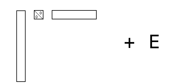
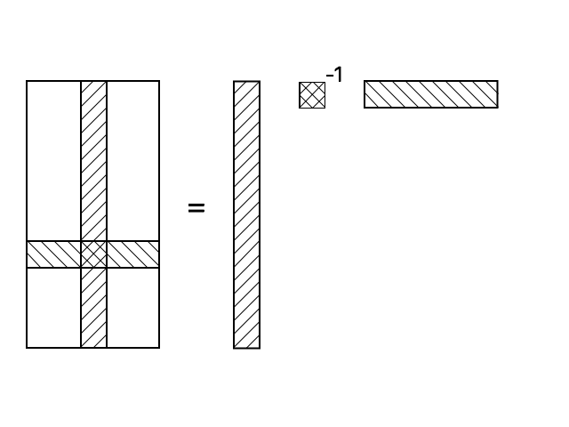
Given an $m\times n$ matrix $M$ of rank $\rho$ and its nonsingular $\rho\times\rho$ submatrix $G=M_{\mathcal{I},\mathcal{J}}$ one can readily verify that $M=M^{\prime}$ for

$$M^{\prime}=CUR,~{}C=M_{:,\mathcal{J}},~{}U=G^{-1},~{}G=M_{\mathcal{I},\mathcal{J}},~{}{\rm and}~{}R=M_{\mathcal{I},:}.$$ (3.1)

We call $G$ the generator and $U$ the nucleus of CUR decomposition of $M$ (see Fig. 3).

Figure 3: CUR decomposition with a nonsingular CUR generator

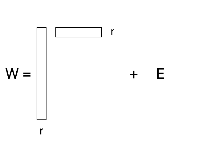
CUR decomposition is extended to CUR approximation of a matrix $M$ close to a rank-$\rho$ matrix (see Fig. 1), although the approximation $M^{\prime}\approx M$ for $M^{\prime}$ of (3.1) can be poor if the generator $G$ is ill-conditioned.

Remark 3.1.

The pioneering papers [22, 21, 23], as well as [19, 20, 18, 52, 34], define CGR approximations having nuclei $G$; “G” can stand, say, for “germ”. We use the acronym CUR, which is more customary in the West. “U” can stand, say, for “unification factor”, but notice the alternatives of CNR, CCR, or CSR with $N$, $C$, and $S$ standing for “nucleus”, “core”, and “seed”.

Zamarashkin and Osinsky proved in [53] that for any matrix $M$ there exists its CUR approximation (3.1) within a factor of $\rho+1$ from optimum under the Frobenius matrix norm, although their proof does not imply a sublinear cost algorithm for computing such a CUR approximation.

Now we face the challenge of devising algorithms that at sublinear cost compute an accurate CUR LRA of a matrix that admits LRA. We refer the reader to [28, 37] for sublinear cost iterative refinement of LRA and heuristic a posteriori error estimates for LRA. In all these studies we generalize LRA of (3.1) by allowing to use $k\times l$ CUR generators for $k$ and $l$ satisfying (2.3) and to choose any $l\times k$ nucleus $U$ for which the error matrix $E=CUR-M$ has smaller norm.

Given two matrices $C$ and $R$, the minimal Frobenius error norm of CUR LRA

$$||E||_{F}=||M-CUR||_{F}\leq||M-CC^{+}M||_{F}+||M-MR^{+}R||_{F}$$

is reached for the nucleus $U=C^{+}MR^{+}$ (see [30, Eqn. (6)]).

We, however, cannot compute such a nucleus at sublinear cost and instead seek canonical CUR LRA (cf. [12, 9, 34]) whose nucleus is the pseudo inverse of the $\rho$-truncation of a given CUR generator:

$$U:=G_{\rho}^{+}.$$ (3.2)

The computation of this nucleus involves only $kl$ memory cells and $O(kl\min\{k,l\})$ flops.

Our study of CUR LRA in this section can be extended to any LRA by means of its transformation into a CUR LRA at sublinear cost (see [37, Sec. 3 and Appendix C]).

3.2 CUR decomposition of a matrix

Theorem 3.1.

[A necessary and sufficient criterion for CUR decomposition.] Let $M^{\prime}=CUR$ be a canonical CUR of $M$ for $U=G_{\rho}^{+}$, $G=M_{\mathcal{I},\mathcal{J}}$. Then $M^{\prime}=M$ if and only if $\operatorname{rank}(G)=\operatorname{rank}(M)$.

Proof.

$\sigma_{j}(G)\leq\sigma_{j}(M)$ for all $j$ because $G$ is a submatrix of $M$. Hence $\epsilon$-rank$(G)\leq\epsilon$-rank$(M)$ for all nonnegative $\epsilon$, and in particular $\operatorname{rank}(G)\leq\operatorname{rank}(M)$.

Now let $M=M^{\prime}=CUR$. Then clearly

$$\operatorname{rank}(M)\leq\operatorname{rank}(U)=\operatorname{rank}(G_{\rho}^{+})=\operatorname{rank}(G_{\rho})\leq\operatorname{rank}(G),$$

Hence

$$\operatorname{rank}(G)\geq\operatorname{rank}(M),~{}{\rm and~{}so}~{}\operatorname{rank}(G)=\operatorname{rank}(M)~{}{\rm if}~{}M^{\prime}=M.$$

It remains to deduce that

$$M=CG_{\rho}^{+}R~{}{\rm if}~{}\operatorname{rank}(G)=\operatorname{rank}(M):=\rho,$$

but in this case $G_{\rho}=G$, and so

$$\operatorname{rank}(CG_{\rho}^{+}R)=\operatorname{rank}(C)=\operatorname{rank}(R)=\rho.$$

Hence the rank-$\rho$ matrices $M$ and $CG_{\rho}^{+}R$ share their rank-$\rho$ submatrices $C$ and $R$. ∎

Remark 3.2.

Can we extend the theorem by proving that $M^{\prime}\approx M$ if and only if $\epsilon$-rank$(G)=\epsilon$-rank$(M)$ for a small positive $\epsilon$? The “only if” claim cannot be extended, e.g., for

$$M=\begin{pmatrix}1&0&0\\ 0&\epsilon&0\\ 0&1&0\end{pmatrix},$$

$\epsilon\approx 0$, and the $2\times 2$ leading submatrix $G$ of $M$. Indeed, $\operatorname{rank}(M)=\operatorname{rank}(G)=2$, and so Thm. 3.1 implies that $M^{\prime}=M$, while $\epsilon$-$\operatorname{rank}(M)=2>\epsilon$-$\operatorname{rank}(G)=1.$

4 Background for random matrix computations

Next we provide background for devising randomized LRA algorithms.

4.1 Gaussian and factor-Gaussian matrices of low rank

Hereafter $\mathbb{E}(w)$ denotes the expected value of random variable $w$, $\stackrel{{\scriptstyle d}}{{=}}$ denotes the equality in distribution, and $\preceq$ and $\succeq$ denote statistically less or equal to and statistically greater or equal to, respectively.

We recall that a random matrix is said to be Gaussian if all its entries are i.i.d. standard Gaussian random variables, and we let $\mathcal{G}^{m\times n}$ denote an $m\times n$ random Gaussian matrix.

Theorem 4.1.

[Nondegeneration of a Gaussian Matrix.] Let $F\stackrel{{\scriptstyle d}}{{=}}\mathcal{G}^{r\times m}$, $H\stackrel{{\scriptstyle d}}{{=}}\mathcal{G}^{n\times r}$, $M\in\mathbb{R}^{m\times n}$, and $r\leq\operatorname{rank}(M)$. Then the matrices $F$, $H$, $FM$, and $MH$ have full rank $r$ with probability 1.

Proof.

Fix any of the matrices $F$, $H$, $FM$, and $MH$ and its $r\times r$ submatrix $B$. Then the equation $\det(B)=0$ defines an algebraic variety of a lower dimension in the linear space of the entries of the matrix because in this case $\det(B)$ is a polynomial of degree $r$ in the entries of the matrix $F$ or $H$ (cf. [6, Proposition 1]). Clearly, such a variety has Lebesgue and Gaussian measures 0, both being absolutely continuous with respect to one another. This implies the theorem. ∎

Assumption 4.1.

[Nondegeneration of a Gaussian matrix.] Throughout this paper we simplify the statements of our results by assuming that a Gaussian matrix has full rank and ignoring the chance for its degeneration, which has probability 0.

Lemma 4.1.

[Orthogonal invariance of a Gaussian matrix.] Suppose that $k$, $m$, and $n$ are three positive integers, $k\leq\min\{m,n\},$ $G\stackrel{{\scriptstyle d}}{{=}}\mathcal{G}^{m\times n}$, $S\in\mathbb{R}^{k\times m}$, $T\in\mathbb{R}^{n\times k}$, and $S$ and $T$ are orthogonal matrices. Then $SG$ and $GT$ are Gaussian matrices.

Definition 4.1.

[Factor-Gaussian matrices.] Suppose that $\rho\leq\min\{m,n\}$,

$$H_{1}\stackrel{{\scriptstyle d}}{{=}}\mathcal{G}^{m\times\rho}~{}{\rm and}~{}H_{2}\stackrel{{\scriptstyle d}}{{=}}\mathcal{G}^{\rho\times n}$$

are two independent random Gaussian matrices, and

$$A\in\mathbb{R}^{m\times\rho},~{}B\in\mathbb{R}^{\rho\times m},~{}{\rm and}~{}\Sigma\in\mathbb{R}^{\rho\times\rho}$$

are full rank well-conditioned constant matrices.

(i) Then we call $AH_{2}$, $H_{1}B$, and $H_{1}\Sigma H_{2}$ right, left, and two-sided factor-Gaussian matrices of rank $\rho$, respectively (cf. Assumption 4.1).

(ii) We refer to small-norm perturbations of factor-Gaussian matrices of rank $\rho$ as to perturbed right, left, and two-sided factor-Gaussian matrices of rank $\rho$ as well as to right, left, and two-sided factor-Gaussian matrices of $\epsilon$-rank $\rho$ for a fixed small positive $\epsilon$.

4.2 Norms of a Gaussian matrix and its pseudo inverse

Hereafter $\Gamma(x)=\int_{0}^{\infty}\exp(-t)t^{x-1}dt$ denotes the Gamma function, and we write

$$\mathbb{E}||M||:=\mathbb{E}(||M||),~{}\mathbb{E}||M||_{F}^{2}:=\mathbb{E}(||M||_{F}^{2}),~{}{\rm and}~{}e:=2.7182818\dots.$$ (4.1)

Definition 4.2.

[Norms of a Gaussian matrix and its pseudo inverse.] Define random variables $\nu_{m,n}\stackrel{{\scriptstyle d}}{{=}}||\mathcal{G}^{m\times n}||$ and $\nu^{+}_{m,n}\stackrel{{\scriptstyle d}}{{=}}||(\mathcal{G}^{m\times n})^{+}||$.

Theorem 4.2.

[Expected norm of a Gaussian matrix.]

$\mathbb{E}(\nu_{m,n})\leq\sqrt{m}+\sqrt{n}$.

Proof.

See [13, Thm. II.7]. ∎

Theorem 4.3.

[Expected norm of the inverse of a Gaussian matrix.]

$\mathbb{E}(\nu^{+}_{m,n})\leq\frac{e\sqrt{m}}{m-n}$ provided that $m\geq n+2\geq 4$.

Proof.

See [24, Eqn. (10.4)]. ∎

Remark 4.1.

[13, Thm. II.7], [8, the proof of Lemma 4.1], [24, Prop. 10.4 and Eqn. (10.3)], and [46, Thm. 3.3] estimate probability distribution of $\nu_{m,n}$ and $\nu^{+}_{m,n}$, but in this paper we already succeed by combining Thms. 4.2 and 4.3 with Markov inequality.

5 A posteriori errors of a canonical CUR LRA

5.1 The Main Result and Outline of a Proof

Outline 5.1.

[Error Estimation for a Canonical CUR LRA.]

1. Consider (but do not compute) an auxiliary $m\times n$ matrix $M^{\prime}$ of rank $\rho$ that approximates the matrix $M$ within a fixed norm bound $\epsilon$, that is,

   $$|M-M^{\prime}|\leq\epsilon.$$ (5.1)

   [We can apply our study to any choice of $M^{\prime}$, e.g., to $M^{\prime}=M_{\rho}$, in which case $||M-M^{\prime}||=\sigma_{\rho+1}(M)$, but in Sec. 6 we assume that $M$ is a norm-$\epsilon$ perturbation of a factor-Gaussian matrix $M^{\prime}$ of Def. 4.1.]

2. Fix a $k\times l$ CUR generator $G^{\prime}=M_{\mathcal{I},\mathcal{J}}^{\prime}$ for the matrix $M^{\prime}$ and define a nucleus $U^{\prime}=G_{\rho}^{\prime+}$ and canonical CUR decomposition $M^{\prime}=C^{\prime}U^{\prime}R^{\prime}$.

3. Observe that

   $$|M-CUR|\leq|M-M^{\prime}|+|M^{\prime}-CUR|\leq\epsilon+|C^{\prime}U^{\prime}R^{\prime}-CUR|.$$ (5.2)

4. Bound the norm $|C^{\prime}U^{\prime}R^{\prime}-CUR|$ in terms of the values $\epsilon$, $|C|$, $|U|$, and $|R|$.

Next we elaborate upon step 4 provided that we have already performed steps 1 – 3.

Theorem 5.1.

Given an $m\times n$ matrix $M$, a $k\times l$ matrix $G:=M_{\mathcal{I},\mathcal{J}}$, a positive integer $\rho<\min\{k,l\}$, a positive number $\epsilon\leq\sigma_{\rho}(G)$, and an $m\times n$ rank $\rho$ matrix $M^{\prime}$ satisfying (5.1), write

$$C:=M_{:,\mathcal{J}},~{}R:=M_{\mathcal{I},:},~{}U=G_{\rho}^{+},~{}v:=\max\{||C||,||R||\}||U||,$$ (5.3)

$$\zeta:=\begin{cases}\sqrt{2}&{\rm for}~{}~{}\rho=\min\{k,l\}\\ (1+\sqrt{5})/2&{\rm for}~{}~{}\rho<\min\{k,l\}\end{cases}$$ (5.4)

and assume that $\sigma_{\rho}(G)>\epsilon$ or equivalently

$$\theta:=\epsilon||U||<1.$$ (5.5)

Then the following inequality holds:

$$||M-CUR||\leq(v+1)\Big{(}\frac{2\zeta}{1-\theta}~{}v+2\Big{)}\epsilon,~{}{\rm where}~{}2\zeta\leq 1+\sqrt{5}~{}{\rm(cf.~{}(\ref{eqzt}))}.$$ (5.6)

5.2 Bound on $|C^{\prime}U^{\prime}R^{\prime}-CUR|$

Lemma 5.1.

Fix the spectral or Frobenius matrix norm $|\cdot|$, five integers $k$, $l$, $m$, $n$, and $\rho$ such that $\rho\leq k\leq m$ and $\rho\leq l\leq n$, an $m\times n$ matrix $M$ having $\epsilon$-rank $\rho$, its rank-$\rho$ approximation $M^{\prime}$ within a norm bound $\epsilon$, such that

$$\tau_{\rho+1}(M)\leq|M^{\prime}-M|\leq\epsilon,$$

and canonical CUR LRAs

$$M\approx CUR~{}{\rm and}~{}M^{\prime}=C^{\prime}U^{\prime}R^{\prime}$$

defined by the same pair of index sets $\mathcal{I}$ and $\mathcal{J}$ of cardinality $k$ and $l$, respectively, such that

$$C:=M_{:,\mathcal{J}},~{}R:=M_{\mathcal{I},:},~{}U=G_{\rho}^{+},~{}~{}C^{\prime}:=M^{\prime}_{:,\mathcal{J}},~{}R^{\prime}:=M^{\prime}_{\mathcal{I},:},~{}U^{\prime}=G_{\rho}^{\prime+},$$

$$G=M_{\mathcal{I},\mathcal{J}},~{}{\rm and}~{}G^{\prime}=M^{\prime}_{\mathcal{I},\mathcal{J}}.$$

Then

$$|C^{\prime}U^{\prime}R^{\prime}-CUR|\leq(|R|+|C^{\prime}|)~{}|U|~{}\epsilon+|C^{\prime}|~{}|R^{\prime}|~{}|U^{\prime}-U|.$$

Proof.

Notice that

$$CUR-C^{\prime}U^{\prime}R^{\prime}=(C-C^{\prime})UR+C^{\prime}U(R-R^{\prime})+C^{\prime}(U-U^{\prime})R^{\prime}.$$

Therefore

$$|CUR-C^{\prime}U^{\prime}R^{\prime}| \leq|C-C^{\prime}|~{}|U|~{}|R|+|C^{\prime}|~{}|U|~{}|R-R^{\prime}|+|C^{\prime}|~{}|U-U^{\prime}|~{}|R^{\prime}|.$$

Substitute the bound $\max\{|C-C^{\prime}|,|R-R^{\prime}|\}\leq|M-M^{\prime}|\leq\epsilon$. ∎

5.3 The Errors of CUR LRA of a Perturbed Matrix of Low Rank

Lemma 5.2.

Under the assumptions of Lemma 5.1 we have

$$||U-U^{\prime}||\leq 2\zeta~{}||U||~{}||U^{\prime}||~{}\epsilon~{}{\rm for}~{}\zeta~{}{\rm of~{}(\ref{eqzt}),~{}such~{}that}~{}2\zeta\leq 1+\sqrt{5}.$$

Proof.

Recall that $\operatorname{rank}(G^{\prime})=\operatorname{rank}(M^{\prime})=\operatorname{rank}(G_{\rho})=\rho$ and that

$$||G^{\prime}-G_{\rho}||\leq||G^{\prime}-G||+||G-G_{\rho}||\leq||M^{\prime}-M||+\sigma_{\rho+1}(M)\leq 2\epsilon.$$

Then apply [3, Thm. 2.2.5] for $A=G,~{}B=G^{\prime}$. ∎

Lemma 5.3.

Under the assumptions of Lemma 5.2 let (5.5) hold. Then $||U^{\prime}||\leq\frac{||U||}{1-\theta}$.

Proof.

Thm. 2.2 implies that

$$\sigma_{\rho}(G^{\prime})\geq\sigma_{\rho}(G)-\epsilon=(1-\epsilon/\sigma_{\rho}(G))\sigma_{\rho}(G)=(1-\epsilon~{}||U||)\sigma_{\rho}(G).$$

Substitute (5.5) and obtain that $\sigma_{\rho}(G^{\prime})\geq(1-\theta)\sigma_{\rho}(G)>0$. Hence

$$||U^{\prime}||=\frac{1}{\sigma_{\rho}(G^{\prime})}\leq\frac{1}{1-\theta}\cdot\frac{1}{\sigma_{\rho}(G)}=\frac{||U||}{1-\theta}.$$

∎

Proof of Thm. 5.1. Write (cf. Lemma 5.1)

$$M^{\prime}:=M_{\rho}:=M^{\prime}_{\mathcal{I},:}{M^{\prime}_{\mathcal{I},\mathcal{J}}}^{+}M^{\prime}_{:,\mathcal{J}},~{}C^{\prime}:=M^{\prime}_{\mathcal{I},:},~{}U^{\prime}:={M^{\prime}_{\mathcal{I},\mathcal{J}}}^{+},~{}R^{\prime}:=M^{\prime}_{:,\mathcal{J}}.$$

Deduce from (5.2) that

$$|M-CUR|\leq\epsilon+|C^{\prime}U^{\prime}R^{\prime}-CUR|.$$

Combine this bound with Lemma 5.1 and obtain that

$$|M-CUR|\leq\epsilon+(|R|+|C^{\prime}|)|U|\epsilon+|C^{\prime}|~{}|R|~{}|U-U^{\prime}|.$$ (5.7)

Lemmas 5.2 and 5.3 together imply that

$$||U-U^{\prime}||\leq\frac{2\zeta}{1-\theta}||U||^{2}\epsilon.$$

Now recall that $|M-M^{\prime}|\leq\epsilon$, and so $||C^{\prime}||\leq||C||+\epsilon$.

Recall that $\epsilon||U||<1$ (cf. (5.5)) and deduce that

$$||C^{\prime}||~{}||U-U^{\prime}||\leq(||C||+\epsilon)\frac{2\zeta}{1-\theta}~{}||U||^{2}\epsilon<\frac{2\zeta}{1-\theta}(||C||~{}|U||^{2}+||U||)\epsilon,$$

and so

$$||C^{\prime}||~{}||R||~{}||U-U^{\prime}||<\frac{2\zeta}{1-\theta}(||R||~{}||C||~{}||U||^{2}+||R||~{}||U||)\epsilon.$$

Substitute $v:=\max\{||C||,||R||\}$ (see (5.3)) and obtain

$$||C^{\prime}||~{}||R||~{}||U-U^{\prime}||<\frac{2\zeta}{1-\theta}(v^{2}+v)\epsilon.$$ (5.8)

Likewise, deduce from the bounds $||C^{\prime}||\leq||C||+\epsilon$ and $\epsilon|U|<1$ that

$$(|R|+|C^{\prime}|)|U|\leq(|R|+|C|+\epsilon|)|U|<(|R|+|C|)|U|+1.$$

Substitute $(\ref{eqv})$ and obtain that $(|R|+|C^{\prime}|)|U|<2v+1$.

Combine this bound with Eqns. (5.7) and (5.8) and obtain the theorem.

6 The errors of CUR LRA of a perturbed factor-Gaussian matrix

In this section we prove that if a matrix $M$ is close to a two-sided factor-Gaussian matrix $M^{\prime}$ of low rank, then a canonical CUR LRA with a generator $G=M_{\mathcal{I},\mathcal{J}}$ is accurate whp for any fixed pair of sufficiently large sets $\mathcal{I}$ and $\mathcal{J}$ of rows and columns indexes.

Write

$$M^{\prime}:=H_{1}\Sigma H_{2}$$ (6.1)

for $H_{1}$, $H_{2}$ , and $\Sigma$ of Def. 4.1 and for $m,n,k,l$, and $\rho$ satisfying

$$k<m,~{}l<n,~{}\textrm{and}~{}\min\{k,l\}\geq\rho+2\geq 4.$$ (6.2)

Recall from (4.1) that $e:=2.7182818\dots$ and define parameters $\alpha$ and $\beta$ as follows:

$$\alpha:=\frac{e^{2}\sqrt{kl}}{(k-\rho)(l-\rho)}~{}\textrm{and}~{}\beta:=\max\big{\{}(\sqrt{m}+\sqrt{\rho})(\sqrt{\rho}+\sqrt{l}),(\sqrt{n}+\sqrt{\rho})(\sqrt{\rho}+\sqrt{k})\big{\}}.$$ (6.3)

Theorem 6.1.

For two Gaussian matrices $H_{1}$ and $H_{2}$, matrices $\Sigma$ and $M^{\prime}$ of (6.1), five integers $k,l,m,n,\rho$ satisfying (6.2), and parameters $\alpha$ and $\beta$ of (6.3), let $\mathcal{I}$ and $\mathcal{J}$ be two fixed row and column index sets such that

$$C^{\prime}=M^{\prime}_{:,\mathcal{J}},~{}R^{\prime}=M^{\prime}_{\mathcal{I},:},~{}G^{\prime}=M^{\prime}_{\mathcal{I},\mathcal{J}}\in\mathbb{R}^{k\times l},~{}{\rm and}~{}U^{\prime}=G^{\prime+}.$$

Then $C^{\prime}$, $R^{\prime}$, and $G^{\prime}$ are factor-Gaussian matrices such that

$$\mathbb{E}||C^{\prime}||\leq(\sqrt{m}+\sqrt{\rho})(\sqrt{\rho}+\sqrt{l})\sigma_{1}(\Sigma)\leq\beta\sigma_{1}(\Sigma),~{}~{}~{}~{}~{}~{}~{}~{}~{}$$

$$\mathbb{E}||R^{\prime}||\leq(\sqrt{n}+\sqrt{\rho})(\sqrt{\rho}+\sqrt{k})\sigma_{1}(\Sigma)\leq\beta\sigma_{1}(\Sigma),~{}~{}~{}~{}~{}~{}~{}~{}~{}$$

$$\mathbb{E}||U^{\prime}||\leq\frac{e^{2}\sqrt{kl}}{(k-\rho)(l-\rho)\sigma_{\rho}(\Sigma)}\leq\frac{\alpha}{\sigma_{\rho}(\Sigma)}~{}~{}~{}~{}~{}~{}~{}~{}~{}~{}~{}~{}~{}~{}~{}~{}~{}~{}~{}~{}~{}$$

for  $e:=2.7182818\dots$ of  (4.1).

Proof.

We estimate $\mathbb{E}||C^{\prime}||$, and one can similarly estimate $\mathbb{E}||R^{\prime}||$.

Recall that $C^{\prime}=M^{\prime}_{:,\mathcal{J}}=H_{1}\Sigma{H_{2}}_{:,\mathcal{J}}$ and that $H_{1}$ and $H_{2}$ are independent of one another and deduce that

$$\mathbb{E}||C^{\prime}|| \leq\mathbb{E}\big{(}||H_{1}||~{}||\Sigma||~{}||{H_{2}}_{:,\mathcal{J}}||\big{)}$$

$$=\sigma_{1}(\Sigma)\mathbb{E}||H_{1}||~{}\mathbb{E}||{H_{2}}_{:,\mathcal{J}}||.$$

Recall from Thm. 4.2 that $\mathbb{E}(\nu_{p,q})\leq\sqrt{p}+\sqrt{q}$ and obtain

$$\mathbb{E}||C^{\prime}||\leq(\sqrt{m}+\sqrt{\rho})(\sqrt{\rho}+\sqrt{l})\sigma_{1}(\Sigma).$$

Next estimate $||U^{\prime}||$. Apply Lemma 2.1, recall from Thm. 4.3 that

$$\mathbb{E}(\nu^{+}_{p,q})\leq\frac{e\sqrt{p}}{p-q},~{}{\rm for}~{}p\geq q+2\geq 2,$$

and deduce that

$$\mathbb{E}||U^{\prime}|| =\mathbb{E}||({H_{1}}_{\mathcal{I},:}\Sigma{H_{2}}_{:,\mathcal{J}})^{+}||$$

$$\leq\mathbb{E}||{H_{1}}_{\mathcal{I},:}^{+}||~{}\mathbb{E}||{H_{2}}_{:,\mathcal{J}}^{+}||~{}/\sigma_{\rho}(\Sigma)$$

$$\leq\frac{e^{2}\sqrt{kl}}{(k-\rho)(l-\rho)\sigma_{\rho}(\Sigma)}=\frac{\alpha}{\sigma_{\rho}(\Sigma)}.$$

∎

Now assume that an input matrix $M$ is a perturbed two-sided factor-Gaussian matrix and that two fixed sets $\mathcal{I}$ and $\mathcal{J}$ of its +row and column indexes are sufficiently large and then prove that whp the generator $G=M_{\mathcal{I},\mathcal{J}}$ is well-conditioned and the norms $||C||$ and $||R||$ are nicely bounded.

Lemma 6.1.

Under the assumptions of Thm. 6.1, let $\epsilon\leq\frac{\sigma_{\rho}(\Sigma)}{30\alpha}$ be a small positive number and let $E\in\mathbb{R}^{m\times n}$ be a perturbation matrix such that $||E||\leq\epsilon$. Write

$$M:=M^{\prime}+E,~{}C:=M_{:,\mathcal{J}},~{}R:=M_{\mathcal{I},;},~{}{\rm and}~{}U:=(M_{\mathcal{I},\mathcal{J}})_{\rho}^{+}.$$

Then with a probability no less than 0.7 we have

$${\rm(i)}~{}~{}~{}~{}~{}~{}~{}~{}~{}~{}~{}~{}~{}~{}~{}~{}~{}~{}~{}~{}~{}~{}~{}~{}~{}~{}~{}~{}~{}~{}~{}~{}~{}~{}~{}~{}~{}~{}~{}~{}~{}||U||\leq\frac{15\alpha}{\sigma_{\rho}(\Sigma)},~{}~{}\epsilon||U||\leq 1/2,~{}~{}~{}~{}~{}~{}~{}~{}~{}~{}~{}~{}~{}~{}~{}~{}~{}~{}~{}~{}~{}~{}~{}~{}~{}~{}~{}~{}~{}~{}~{}$$

$${\rm(ii)}~{}~{}~{}~{}~{}~{}~{}~{}~{}~{}~{}~{}~{}~{}~{}~{}~{}~{}~{}~{}~{}~{}~{}~{}~{}~{}~{}\max\{||C||,||R||\}||U||\leq 150\alpha\beta\sigma_{1}(\Sigma)/\sigma_{\rho}(\Sigma)+1/2.~{}~{}~{}~{}~{}~{}~{}~{}~{}~{}~{}~{}~{}~{}~{}~{}~{}~{}$$

Proof.

(i) By combining the bound of Thm. 6.1 on the expected norm $\mathbb{E}||U^{\prime}||$ with Markov’s inequality, deduce that

$$||U^{\prime}||\leq\frac{10\alpha}{\sigma_{\rho}(\Sigma)}\textrm{ or equivalently }\sigma_{\rho}(M^{\prime}_{\mathcal{I},\mathcal{J}})\geq\frac{\sigma_{\rho}(\Sigma)}{10\alpha}$$ (6.4)

with a probability no less than 0.9.

Similarly to the argument of Lemma 5.3, deduce that

$$\sigma_{\rho}(M_{\mathcal{I},\mathcal{J}})\geq\sigma_{\rho}(M^{\prime}_{\mathcal{I},\mathcal{J}})-\epsilon\geq\frac{\sigma_{\rho}(\Sigma)}{15\alpha},$$

and then claim (i) follows.
(ii) By combining the bounds of Thm. 6.1 on the expected norms $\mathbb{|}|C^{\prime}||$ and $\mathbb{|}|R^{\prime}||$ with Markov’s inequality and the bound on the probability of a union of random variables, obtain that

$$\max\big{\{}||C||,||R||\big{\}}\leq 10\beta\sigma_{1}(\Sigma)+\epsilon$$

with a probability no less than 0.8. Then combine claim (i) with the union bound and obtain that

$$\max\{||C||,||R||\}||U||\leq 150\alpha\beta\sigma_{1}(\Sigma)/\sigma_{\rho}(\Sigma)+1/2$$

with a probability no less than 0.7. ∎

Now choose any generator of CUR LRA of a perturbed factor-Gaussian matrix of rank $\rho$ and prove a probabilistic upper bound on the error of a resulting CUR LRA of that matrix.

Theorem 6.2.

If the assumptions of Lemma 6.1 hold for a perturbed factor-Gaussian matrix $M$, then bound (5.6) on the approximation error norm $||M-CUR||$ for $\theta\leq 1/2$, that is,

$$||M-CUR||\leq(4\zeta v+2)(v+1)\epsilon,~{}{\rm for}~{}4\zeta\leq 2+2\sqrt{5},~{}v=150\alpha\beta\sigma_{1}(\Sigma)/\sigma_{\rho}(\Sigma)+1/2,$$ (6.5)

holds with a probability no less than 0.6.

Proof.

Combine the assumption of Lemma 6.1 that $\epsilon\leq\frac{\sigma_{\rho}(\Sigma)}{30\alpha}$ with bound (6.4) of that lemma and conclude that with a probability $p_{0}\geq 0.9$, the bound $\sigma_{\rho}(G)\geq 3\epsilon>\epsilon$ and therefore (5.6) hold. Replace $\theta$ and $v$ with their upper bounds 1/2 and $150\alpha\beta\sigma_{1}(\Sigma)/\sigma_{\rho}(\Sigma)+1/2$, respectively, which hold with a probability $p_{1}\geq 0.7$. Combine the bounds $p_{0}\leq 0.9$ and $p_{1}\leq 0.7$. ∎

Remark 6.1.

Recall that

$$\alpha:=\frac{e^{2}\sqrt{kl}}{(k-\rho)(l-\rho)}~{}{\rm and}~{}\beta:=\max\big{\{}(\sqrt{m}+\sqrt{\rho})(\sqrt{\rho}+\sqrt{l}),(\sqrt{n}+\sqrt{\rho})(\sqrt{\rho}+\sqrt{k})\big{\}}.$$

Furthermore, suppose that $m\gg k\gg\rho$, $n\gg l\gg\rho$, and

$$v=150\alpha\beta\sigma_{1}(\Sigma)/\sigma_{\rho}(\Sigma)+1/2=O\Big{(}\max\Big{\{}\frac{\sqrt{m}}{\sqrt{k}},\frac{\sqrt{n}}{\sqrt{l}}\Big{\}}\Big{)}.$$

Now drop the smaller terms of (6.5), and obtain that its dominant part is

$$O\Big{(}\max\Big{\{}\frac{m}{k},\frac{n}{l}\Big{\}}\cdot\epsilon\Big{)}.$$

7 CUR LRA algorithms running at sublinear cost

7.1 Primitive and Cynical algorithms

Given an $m\times n$ matrix $M$ admitting close rank-$\rho$ approximation and a pair of $k$ and $l$ satisfying (2.3), define a canonical CUR LRA of $M$ by fixing or choosing at random a pair of sets $\mathcal{I}$ and $\mathcal{J}$ of $k$ row and $l$ column indexes, respectively, and call the resulting algorithm Primitive. Apart from the selection of the sets $\mathcal{I}$ and $\mathcal{J}$ the algorithm amounts to computing the $\rho$-truncation $(M_{\mathcal{I},\mathcal{J}})_{\rho}$ of the matrix $M_{\mathcal{I},\mathcal{J}}$ and its pseudo inverse $((M_{\mathcal{I},\mathcal{J}})_{\rho})^{+}$ at the overall arithmetic cost in $O(kl\min\{k,l\})$. This cost bound is sublinear if $kl\min\{k,l\}\ll mn$.

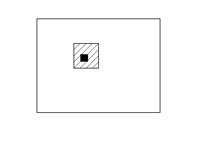
Thm. 5.1 shows that the norms of the nucleus and output errors of the algorithm tend to decrease as we expand the sets $\mathcal{I}$ and $\mathcal{J}$ of $k$ rows and $l$ columns defining a CUR generator $G$. Likewise, our estimates for the norm $||M-CUR||$ relying on Remark 6.1 in the case of perturbed factor-Gaussian input matrix $M$ are roughly proportional to the value $\max\Big{\{}\frac{m}{k},\frac{n}{l}\Big{\}}$. These observations motivate our design of the following CUR LRA algorithm, which we call Cynical(see Fig. 4).

Figure 4: A cynical CUR algorithm (the strips mark a $p\times q$ submatrix; a $k\times l$ CUR generator is shown in black)

Algorithm 7.1.

For an $m\times n$ factor-Gaussian matrix $M$ of rank $\rho$, fix four integers $k$, $l$, $p$, and $q$ such that

$$0<\rho\leq k\leq p\leq m~{}{\rm and}~{}\rho\leq l\leq q\leq n,$$ (7.1)

fix or choose at random a pair of sets $\mathcal{I}$ and $\mathcal{J}$ of $p$ row and $q$ column indexes, respectively, compute a $k\times l$ CUR generator $G_{k,l}$ for the $p\times q$ submatrix $M_{\mathcal{I},\mathcal{J}}$ of $M$ by applying to $M_{\mathcal{I},\mathcal{J}}$ the algorithms of [16] or [35], compute the $\rho$-truncation $G_{k,l,\rho}$, and build on it CUR LRA of $M$.

The algorithm still involves computation of $\rho$-truncation of a $k\times l$ CUR generator and its pseudo inverse, but the arithmetic cost $O(kl\min\{k,l\})$ of this computation is dominated by the cost $O(pq\min\{p,q\})$ of performing the algorithms of [16] or [35], which is still sublinear if we choose sufficiently small integers $p$ and $q$ such that $pq\min\{p,q\}\ll mn$.

The two-stage choice of the CUR generator in a cynical algorithm should decrease the error norm, but application of the algorithms of [16] or [35] can increase the output error bound of Alg. 7.1 by a factor of $\sqrt{(p-k)(q-l)kl}$.

For smaller positive integers $p$ and $q$ and $k=l=\rho$ instead of the algorithms of [16] or [35], one can apply exhaustive search for a $\rho\times\rho$ submatrix of a fixed $p\times q$ submatrix $M_{p,q}$ of $M$ such that CUR LRA built on that submatrix as a CUR generator minimizes the Frobenius error norm $||M-CUR||_{F}$. Zamarashkin and Osinsky proved in [53] that up to a factor of $\rho+1$ this CUR LRA reaches minimal error norm $\sigma_{F,\rho+1}(M_{p,q})$ of Thm. 2.1 for any LRA of $M$.

This exhaustive search should be performed over $\begin{pmatrix}p\\ \rho\end{pmatrix}\begin{pmatrix}q\\ \rho\end{pmatrix}$ candidate $\rho\times\rho$ submatrices of $M_{p,q}$ at sublinear cost of $\begin{pmatrix}p\\ \rho\end{pmatrix}\begin{pmatrix}q\\ \rho\end{pmatrix}C(m,n,\rho)\ll mn$ where $C(m,n,\rho)$ denotes the cost of the estimation of the error norm of CUR LRA of $M$ for a fixed $\rho\times\rho$ CUR generator. This cost is not sublinear even for the matrices of the small family of the Appendix, but one can apply various sublinear cost heuristics.

7.2 Cross-Approximation (C–A) iterations

Apply Cynical algorithm for $p=m$ and $q^{2}\ll n$ or $q=n$ and $p^{2}\ll m$, that is, choose a $p\times q$ submatrix made up of a small number of columns or rows of an $m\times n$ input matrix $M$. Notice that the algorithm still runs at sublinear cost and ensures quite favorable bounds on its output errors.

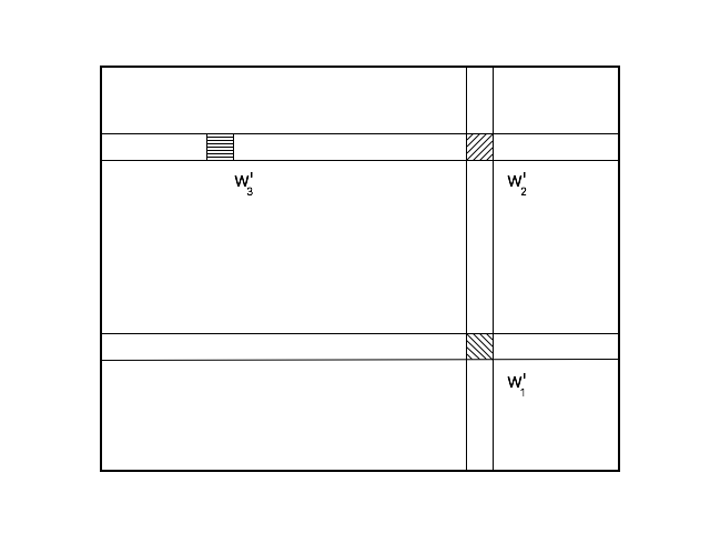
Recursively alternate such choices of horizontal and vertical CUR generators to arrive at the following Cross-Approximation (C–A) iterations (see Fig. 5), specified below.

C-A iterations.

• For an $m\times n$ matrix $M$ and target rank $r$, fix four integers $k$, $l$, $p$ and $q$ satisfying (7.1). [C-A iterations are simplified in a special case where $p:=k$ and $q:=l$.]

• Fix an $m\times q$ “vertical” submatrix of the matrix $M$, made up of its $q$ columns.

• By applying a fixed CUR LRA subalgorithm, e.g., one of the algorithms of [33, 16, 35, 12], compute a $k\times l$ CUR generator $G$ of this submatrix and reuse it for the matrix $M$.

• Output the resulting CUR LRA of $M$ if it is close enough.

• Otherwise swap $p$ and $q$ and reapply the algorithm to the matrix $M^{*}$.

  [This is equivalent to computing a $k\times l$ CUR generator of a fixed $p\times n$ “horizontal” submatrix $M_{1}$ of $M$ that covers the submatrix $G$.]

• Recursively alternate such “vertical” and “horizontal” steps until an accurate CUR LRA is computed or until the number of recursive C–A steps exceeds a fixed tolerance bound.

Figure 5: The first three recursive C–A steps output three striped submatrices.

Initialization recipes. For a large class of input matrices it is efficient to apply adaptive C-A iterations (cf. [1, 2, 4, 5]). They combine initialization with dynamic search for gaps in the singular values of $M$ by properly adapting Gaussian elimination with pivoting. The alternative initialization in [18] uses $O(n\rho^{2})$ flops to initialize the C–A iterations for an $n\times n$ input and $q=s=\rho$, and then the algorithm uses $O(\rho n)$ flops per C–A step.

7.3 Volume maximization and CUR LRA

We devised C-A iterations by extending cynical algorithms towards bounding the norm of the nucleus, but success of C-A iterations in [18, 34, 33] largely relied on maximization of the volume or projective volume at every C-A step (see Thm. 7.1 below)).

Definition 7.1.

For three integers $k$, $l$, and $r$ such that $1\leq r\leq\min\{k,l\}$, define the volume $v_{2}(M):=\prod_{j=1}^{\min\{k,l\}}\sigma_{j}(M)$ of a $k\times l$ matrix $M$ and its $r$-projective volume $v_{2,r}(M):=\prod_{j=1}^{r}\sigma_{j}(M)$ such that $v_{2,r}(M)=v_{2}(M)~{}{\rm if}~{}r=\min\{k,l\}$, $v_{2}^{2}(M)=\det(MM^{*})$ if $k\geq l$; $v_{2}^{2}(M)=\det(M^{*}M)$ if $k\leq l$, $v_{2}^{2}(M)=|\det(M)|^{2}$ if $k=l$.

Given a matrix $W$, five integers $k$, $l$, $m$, $n$, and $r$ such that $1\leq r\leq\min\{k,l\}$, and a real $h>1$, and an $m\times n$ matrix $W$, its $k\times l$ submatrix $G$ has weakly $h$-maximal volume (resp. $r$-projective volume) in $W$ if $v_{2}(G)$ (resp. $v_{2,r}(G)$) is maximal up to a factor of $h$ among all $k\times l$ submatrices of $W$ that differ from $G$ in a single row and/or a single column. We write maximal for $1$-maximal and drop “weakly” if the volume maximization is over all submatrices of a fixed size $k\times l$.

For an $m\times n$ matrix $W=(w_{i,j})_{i,j=1}^{m,n}|$ define its Chebyshev norm $||W||_{C}:=\max_{i,j=1}^{m,n}|w_{ij}|$ such that (cf. [17])

$$||W||_{C}\leq||W||_{2}\leq||W||_{F}\leq\sqrt{mn}~{}||W||_{C}.$$ (7.2)

Recall the following result from [34]:

Theorem 7.1.

Suppose that $W_{k,l}=W_{\mathcal{I},\mathcal{J}}$ is a $k\times l$ submatrix of an $m\times n$ matrix $W$, $U=W_{k,l,r}^{+}$ is the canonical nucleus of a CUR LRA of $W$, $E=W-CUR$, $h\geq 1$, and the $r$-projective volume of $W_{\mathcal{I},\mathcal{J}}$ is locally $h$-maximal. Then

$$||E||_{C}\leq h~{}f(k,l,r)~{}\sigma_{r+1}(W)~{}~{}{\rm for}~{}~{}f(k,l,r):=\sqrt{\frac{(k+1)(l+1)}{(k-r+1)(l-r+1)}}.$$

In particular if $r=\min\{k,l\}$, then the $r$-projective volume turns into volume and

$$f(k,l,r):=\sqrt{\frac{(k+1)(l+1)}{(|l-k|+1)}}.$$

8 Multiplicative pre-processing and generation of multipliers

8.1 Recursive multiplicative pre-processing for LRA

We proved that Primitive, Cynical, and C-A algorithms, running at sublinear cost, output quite accurate CUR LRA whp on random input matrix that admits sufficiently close LRA, thus suggesting that the algorithms output accurate LRA for many and in a sense most of dense matrices admitting sufficiently close LRA. These results do not apply to a non-random real world matrix admitting close LRA. We can, however, boost the likelihood of producing accurate LRA if we recursively apply the same algorithms to various independently generated matrices $M^{(i)}$, $i=1,2,\dots$, whose LRA can be readily transformed into LRA of an original matrix $M$. To define pairwise independent multipliers we generate them by using randomization of some kind (see the next subsection).

Now let $M^{(i)}=X^{(i)}MY^{(i)}$, $i=1,2,\dots$, for some pairs of square orthogonal matrices $X^{(i)}$ and $Y^{(i)}$. For every $i$ one of $X_{i}$ and $Y_{i}$ can be the identity matrix, but the other matrices $X_{i}$ and $Y_{i}$ should be chosen independently of each other. We stop this process as soon as we obtain a reasonable LRA $A^{(i)}B^{(i)}\approx M^{(i)}=X^{(i)}MY^{(i)}$ (this stopping criterion may rely on a posteriori error estimates of [37]). Then we can immediately obtain LRA $X^{(i)*}A^{(i)}B^{(i)}Y^{(i)*}\approx M$ such that $|X^{(i)*}A^{(i)}B^{(i)}Y^{(i)*}-M|=|AB-M^{(i)}|$.

We can compute the matrices $M^{(i)}$ and then shift from the LRA $A^{(i)}B^{(i)}$ of $M^{(i)}$ to LRA $X^{(i)*}A^{(i)}B^{(i)}Y^{(i)*}$ of $M$ at sublinear cost by choosing sufficiently sparse multipliers $A^{(i)}$ and $B^{(i)}$. We can further decrease the computational cost when we seek CUR LRA $X^{(i)}MY^{(i)}=C^{(i)}U^{(i)}R^{(i)}$ because $C^{(i)}=(X^{(i)}MY^{(i)})_{:,\mathcal{J}_{i}}=X^{(i)}M~{}(Y^{(i)})_{:,\mathcal{J}_{i}}$, $R^{(i)}=(X^{(i)}MY^{(i)})_{\mathcal{I}_{i},:}=(X^{(i)})_{\mathcal{I}_{i},:}~{}MY^{(i)}$, and $G^{(i)}=(X^{(i)}MY^{(i)})_{\mathcal{I}_{i},\mathcal{J}_{i}}=(X^{(i)})_{\mathcal{I}_{i},:}~{}M~{}(Y^{(i)})_{:,\mathcal{J}_{i}}$ (a CUR generator), and so we can use rectangular submatrices of $X^{(i)}$ and $Y^{(i)}$ as multipliers.

8.2 Gaussian pre-processing

Next we prove that pre-processing with Gaussian multipliers $X$ and $Y$ transforms any matrix that admits LRA into a perturbation of a factor-Gaussian matrix.

Theorem 8.1.

Consider five integers $k$, $l$, $m$, $n$, and $\rho$ satisfying (2.3), an $m\times n$ well-conditioned matrix $M$ of rank $\rho$, $k\times m$ and $n\times l$ Gaussian matrices $G$ and $H$, respectively, and the norms $\nu_{p,q}$ and $\nu_{p,q}^{+}$ of Def. 4.2. Then

(i) $GM$ is a left factor-Gaussian matrix of rank $\rho$ such that

$$||GM||\preceq||M||~{}\nu_{k,\rho}~{}{\rm and}~{}||(GM)^{+}||\preceq||M^{+}||~{}\nu_{k,\rho}^{+},$$

(ii) $MH$ is a right factor-Gaussian matrix of rank $\rho$ such that

$$||MH||\preceq||M||~{}\nu_{\rho,l}~{}{\rm and}~{}||(MH)^{+}||\preceq||M^{+}||~{}\nu_{\rho,l}^{+},$$

(iii) $GMH$ is a two-sided factor-Gaussian matrix of rank $\rho$ such that

$$||GMH||\preceq||M||~{}\nu_{k,\rho}\nu_{\rho,l}~{}{\rm and}~{}||(GMH)^{+}||\preceq||M^{+}||~{}\nu_{k,\rho}^{+}\nu_{\rho,l}^{+}.$$

Proof.

Let $M=S_{M}\Sigma_{M}T^{*}_{M}$ be SVD where $\Sigma_{M}$ is the diagonal matrix of the singular values of $M$; it is well-conditioned since so is the matrix $M$. Then $\bar{G}:=GS_{M}$ and $\bar{H}:=T_{M}^{*}H$ are Gaussian matrices by virtue of Lemma 4.1, which states orthogonal invariance of Gaussian matrices: indeed in our case $G$ and $H$ are Gaussian, while $S_{M}\in\mathbb{R}^{m\times\rho}$ and $T_{M}\in\mathbb{R}^{\rho\times n}$ are orthogonal matrices. Furthermore

(i) $GM=\bar{G}\Sigma_{M}T_{M}^{*}=\bar{G}_{\rho}\Sigma_{M}T_{M}^{*}$,

(ii) $MH=S_{M}\Sigma_{M}\bar{H}=S_{M}\Sigma_{M}\bar{H}_{\rho}$,

(iii) $GMH=\bar{G}\Sigma_{M}\bar{H}=\bar{G}_{\rho}\Sigma_{M}\bar{H}_{\rho}$ where $\rho\leq\min\{m,n\}$, and

(iv) $\bar{G}_{\rho}=\bar{G}\begin{pmatrix}I_{\rho}\\ O\end{pmatrix}$, and $\bar{H}_{\rho}=(I_{\rho}~{}|~{}O)\bar{H}$.

Combine the latter claims (i)–(iv) with Lemma 2.1. ∎

8.3 Randomized pre-processing

By virtue of Thm. 8.1 multiplication by Gaussian matrices turns any matrix admitting its close LRA into a perturbed factor-Gaussian matrix, whose close LRA we can compute at sublinear cost by virtue of our results of Sec. 6. We can prove similar results by means of applying or extending the techniques of [24, Secs. 10 and 11], [49, 10] in the cases where the multipliers are Rademacher’s, SRHT, or SRFT matrices; the latter matrices have been defined by Hadamard and Fourier transforms, respectively. Multiplication by all these multipliers is performed at superlinear cost, but we conjecture that the same algorithms should output close LRA of a matrix that admits its LRA and is pre-processsed at sublinear cost with sparse orthogonal multipliers; our tests with both synthetic and real world inputs are in good accordance with this conjecture.

In the next subsection we recall generation of $2^{t}\times 2^{t}$ SRHT and SRFT dense matrices in $t$ recursive steps and consider abridged processes consisting in $d<t$ steps, which for smaller positive integers $d$ define sparse orthogonal matrices that have precisely $2^{d}$ nonzero entries in each row and each column.

We turn them into sparse rectangular orthogonal multipliers (said to be abridged scaled and permuted multipliers) by means of multiplying Rademacher’s or random unitary diagonal scaling and multiplication by subpermutation matrices, that is, full rank submatrices of random permutation matrices. The results of our tests with these multipliers turned out to be in good accordance with our conjecture above.

Another promising class of sparse multipliers is given by randomly scaled random subpermutation matrices.

To strengthen the chances for success with sparse pre-processing at sublinear cost one can first combine a small number of distinct multipliers into a single multiplier given by their sum, their linear combination, or more generally a small degree polynomial and then orthogonalize the resulting matrix.

8.4 Multipliers derived from Rademacher’s, Hadamard and Fourier matrices

Every entry of a Rademacher’s matrix is filled with 1 and $-1$ chosen with equal probability 1/2 independently of other entries. We define a square sparse quasi Rademacher’s matrix by first filling its diagonal in this way and filling other entries with 0s, and then successively changing some of its non-diagonal entries into 1 or $-1$, each time chosen with equal probability 1/2. While recursively generating these sparse matrices we can periodically use them as multipliers in a fixed LRA algorithm and every time verify whether the output LRA already satisfies a fixed stopping criterion.

We generate quasi SHRT and SRFT multipliers by abridging the classical recursive processes of the generation of $n\times n$ SRHT and SRFT matrices in $t=\log_{2}(n)$ recursive steps for $n=2^{t}$. Our abridged processes have recursive depth $d\leq t$, begin with the $2^{t-d}\times 2^{t-d}$ identity matrix $H_{0}=F_{0}=I_{2^{t-d}}$, and recursively generate the following matrices:

$$H_{i+1}=\begin{pmatrix}H_{i}&H_{i}\\ H_{i}&-H_{i}\end{pmatrix}~{}{\rm and}~{}F_{i+1}=\widehat{P}_{i+1}\begin{pmatrix}F_{i}&~{}~{}F_{i}\\ F_{i}\widehat{D}_{i}&-F_{i}\widehat{D}_{i}\end{pmatrix},$$

where

$$\widehat{D}_{i}=\operatorname{diag}(\omega_{2^{i}}^{j})_{j=0}^{2^{i-1}-1},~{}\omega_{2^{i}}=\exp(2\pi\sqrt{-1}/2^{i}),$$

$\widehat{P}_{i}$ is the matrix of odd/even permutations such that $\widehat{P}_{i+1}({\bf u})={\bf v}$, ${\bf u}=(u_{j})_{j=0}^{2^{i+1}-1}$, ${\bf v}=(v_{j})_{j=0}^{2^{i+1}-1}$, $v_{j}=u_{2j}$, $v_{j+2^{i}}=u_{2j+1}$, $j=0,1,\ldots,2^{i}-1$, and $i=0,1,\dots,d-1$.

For $s:=2^{t-d}=n/2^{d}$ and $d=1,2,3$ we obtain the following expressions:

$$H_{1}=F_{1}=\begin{pmatrix}I_{s}&I_{s}\\ I_{s}&-I_{s}\end{pmatrix},~{}H_{2}=\begin{pmatrix}I_{s}&I_{s}&I_{s}&I_{s}\\ I_{s}&-I_{s}&I_{s}&-I_{s}\\ I_{s}&I_{s}&-I_{s}&-I_{s}\\ I_{s}&-I_{s}&-I_{s}&I_{s}\end{pmatrix},~{}F_{2}=\begin{pmatrix}I_{s}&I_{s}&I_{s}&I_{s}\\ I_{s}&{\bf i}I_{s}&-I_{s}&-{\bf i}I_{s}\\ I_{s}&-I_{s}&I_{s}&-I_{s}\\ I_{s}&-{\bf i}I_{s}&-I_{s}&{\bf i}I_{s}\end{pmatrix},$$

$$H_{3}=\begin{pmatrix}I_{s}&I_{s}&I_{s}&I_{s}&I_{s}&I_{s}&I_{s}&I_{s}\\ I_{s}&-I_{s}&I_{s}&-I_{s}&I_{s}&-I_{s}&I_{s}&-I_{s}\\ I_{s}&I_{s}&-I_{s}&-I_{s}&I_{s}&I_{s}&-I_{s}&-I_{s}\\ I_{s}&-I_{s}&-I_{s}&I_{s}&I_{s}&-I_{s}&-I_{s}&I_{s}\\ I_{s}&I_{s}&I_{s}&I_{s}&-I_{s}&-I_{s}&-I_{s}&-I_{s}\\ I_{s}&-I_{s}&I_{s}&-I_{s}&-I_{s}&I_{s}&-I_{s}&I_{s}\\ I_{s}&I_{s}&-I_{s}&-I_{s}&-I_{s}&-I_{s}&I_{s}&I_{s}\\ I_{s}&-I_{s}&-I_{s}&I_{s}&-I_{s}&I_{s}&I_{s}&-I_{s}\end{pmatrix},$$

$$~{}F_{3}=\begin{pmatrix}I_{s}&I_{s}&I_{s}&I_{s}&I_{s}&I_{s}&I_{s}&I_{s}\\ I_{s}&\omega_{8}I_{s}&{\bf i}I_{s}&{\bf i}\omega_{8}I_{s}&-I_{s}&-\omega_{8}I_{s}&-{\bf i}I_{s}&-{\bf i}\omega_{8}I_{s}\\ I_{s}&{\bf i}I_{s}&-I_{s}&-{\bf i}I_{s}&I_{s}&{\bf i}I_{s}&-I_{s}&-{\bf i}I_{s}\\ I_{s}&{\bf i}\omega_{8}I_{s}&-{\bf i}&\omega_{8}I_{s}&-I_{s}&-{\bf i}\omega_{8}I_{s}&{\bf i}I_{s}&-\omega_{8}I_{s}\\ I_{s}&-I_{s}&I_{s}&-I_{s}&I_{s}&-I_{s}&I_{s}&-I_{s}\\ I_{s}&-\omega_{8}I_{s}&{\bf i}I_{s}&-{\bf i}\omega_{8}I_{s}&-I_{s}&\omega_{8}I_{s}&-{\bf i}I_{s}&{\bf i}\omega_{8}I_{s}\\ I_{s}&-{\bf i}I_{s}&-I_{s}&{\bf i}I_{s}&I_{s}&-{\bf i}I_{s}&-I_{s}&{\bf i}I_{s}\\ I_{s}&-\omega_{8}I_{s}&-{\bf i}I_{s}&-\omega_{8}I_{s}&-I_{s}&\omega_{8}I_{s}&{\bf i}I_{s}&\omega_{8}I_{s}\end{pmatrix}.$$

For every $d$, the matrix $H_{d}$ is orthogonal and the matrix $F_{d}$ is unitary up to scaling by $2^{-d/2}$. For $d=t$ the matrix $H_{0}=F_{0}$ turns into scalar 1, and we recursively define the matrices of Walsh-Hadamard and discrete Fourier transforms (cf. [29] and [36, Sec. 2.3]).

Incorporating our pre-processing into Primitive algorithms, we restrict multiplication to $k\times m$ or $n\times l$ submatrices $H_{k,t}$ and $H_{t,l}$ of $H_{t}$ and $F_{k,t}$ and $F_{t,l}$ of $F_{t}$.

We perform computations with $H_{d}$ and $F_{d}$ at sublinear cost by stopping where the integer $t-d$ is not small. Namely, for every $d$, the matrices $H_{d}$ and $F_{d}$ have $2^{d}$ nonzero entries in every row and column. Consequently, we can compute the matrices $H_{k,d}M$ and $MH_{d,l}$ by using less than $2^{d}kn$ and $2^{d}ml$ additions and subtractions, respectively, and can compute the matrices $F_{k,d}M$ and $MF_{d,l}$ by using $O(2^{d}kn)$ and $O(2^{d}ml)$ flops, respectively.

By choosing at random $k$ rows or $l$ columns of a matrix $H_{d}$ or $F_{d}$ for $\rho\leq k\leq n$ and $\rho\leq l\leq n$, respectively, and then applying Rademacher’s or random unitary diagonal scaling, we obtain a $d$-abridged scaled and permuted matrix of Hadamard or Fourier transform, respectively, which turn into an SRHT or SRFT matrix for $d=t$.

For $k$ and $l$ of order $r\log(r)$ the superlinear cost algorithms of [24, Sec. 11] with a SRHT or SRFT multiplier output whp nearly optimal LRA of any matrix $M$ that admits LRA, but in our tests the output was usually quite accurate even with sparse 3-abridged scaled and permuted matrices of Hadamard and Fourier transforms, computed at sublinear cost in three recursive steps. Combinations of such matrices with subpermutation matrices via sums, products, and other low degree polynomials turned out to define quite reliable low-cost pre-processing according to our tests.

8.5 Subspace Sampling Variation of the Primitive Algorithm

The computation of a $k\times l$ CUR generator for a pre-processed $m\times n$ matrix $XMY$ with rectangular matrices $X\in\mathbb{R}^{k\times m}$ and $Y\in\mathbb{R}^{n\times l}$ can be equivalently represented as a modification of the Primitive algorithm. It can be instructive to specify this representation.

Subspace Sampling Variation of the Primitive Algorithm:

Successively compute

(i) the matrix $XMY$ for two fixed or random multipliers (aka test matrices) $X\in\mathbb{R}^{k\times m}$ and $Y\in\mathbb{R}^{n\times l}$,

(ii) the Moore – Penrose pseudo inverse $N=((XMY)_{\rho})^{+}$ of its $\rho$-truncation,

(iii) a rank-$\rho$ approximation $MYNXM$ of the matrix $M$.

Our analysis and in particular our error estimation are readily extended to this modification of the Primitive algorithm. Observe its similarity to subspace sampling algorithm of [50] (whose origin can be traced back to [51]) and those of [41] but notice that in the algorithms of [50], [51], and [41] the stage of $\rho$-truncation is replaced by the orthogonalization of the matrix $MH$.

9 Numerical experiments

9.1 Test overview

Next we present our tests of Primitive, Cynical, and C–A algorithms for CUR LRA of both synthetic and real world input matrices. Our tests have confirmed very high efficiency of C-A iterations already where they are performed at sublinear cost, in accordance to and even beyond our formal support. Moreover, their power was impressively strong even without using adaptive techniques of [1]. The tests also showed potentials of obtaining accurate LRA at sublinear cost by means of Primitive and Cynical algorithms for a large input class.

We have performed the tests in the Graduate Center of the City University of New York by using MATLAB. In particular we applied its standard normal distribution function ”randn()” to generate Gaussian matrices and calculated $\epsilon$-ranks of matrices for $\epsilon=10^{-6}$ by using the MATLAB’s function ”rank(-,1e-6)”, which only counts singular values greater than $10^{-6}$.

Our tables display the mean value of the spectral norm of the relative output error over 1000 runs for every class of inputs as well as the standard deviation (std) except where it is indicated otherwise. Some numerical experiments were executed with software custom programmed in $C^{++}$ and compiled with LAPACK version 3.6.0 libraries.

9.2 Input matrices for LRA

We used the following three classes of input matrices $M$ for testing LRA algorithms.

Class I (Synthetic inputs): Perturbed $n\times n$ factor-Gaussian matrices with expected rank $r$, that is, matrices $W$ in the form

$$M=G_{1}*G_{2}+10^{-10}G_{3},$$

for three Gaussian matrices $G_{1}$ of size $n\times r$, $G_{2}$ of size $r\times n$, and $G_{3}$ of size $n\times n$.

Class II: The dense matrices with smaller ratios of “$\epsilon$-rank/$n$” from the built-in test problems in Regularization Tools, which came from discretization (based on Galerkin or quadrature methods) of the Fredholm Integral Equations of the first kind, namely to the following six input classes from the Database:

baart: Fredholm Integral Equation of the first kind,

shaw: one-dimensional image restoration model,

gravity: 1-D gravity surveying model problem,

wing: problem with a discontinuous solution,

foxgood: severely ill-posed problem,

inverse Laplace: inverse Laplace transformation.

9.3 Four algorithms used

In our tests we applied and compared the following four algorithms for computing CUR LRA to input matrices $M$ having $\epsilon$-rank $r$:

• Tests 1 (The Primitive algorithm for $k=l=r$): Randomly choose two index sets $\mathcal{I}$ and $\mathcal{J}$, both of cardinality $r$, then compute a nucleus $U=M_{\mathcal{I},\mathcal{J}}^{-1}$ and define CUR LRA

  $$\tilde{M}:=CUR=M_{:,\mathcal{J}}\cdot M_{\mathcal{I},\mathcal{J}}^{-1}\cdot M_{\mathcal{I},\cdot}.$$ (9.1)

• Tests 2 (Five loops of C–A): Randomly choose an initial row index set $\mathcal{I}_{0}$ of cardinality $r$, then perform five loops of C–A by applying Alg. 1 of [35] as a subalgorithm that produces $r\times r$ CUR generators. At the end compute a nucleus $U$ and define CUR LRA as in Tests 1.

• Tests 3 (A Cynical algorithm for $p=q=4r$ and $k=l=r$): Randomly choose a row index set $\mathcal{K}$ and a column index set $\mathcal{L}$, both of cardinality $4r$, and then apply Algs. 1 and 2 from [35] in order to compute a $r\times r$ submatrix $M_{\mathcal{I},\mathcal{J}}$ of $M_{\mathcal{K},\mathcal{L}}$. Compute a nucleus and obtain CUR LRA by applying equation (9.1).

• Tests 4 (Combination of a single C–A loop with Tests 3): Randomly choose a column index set $\mathcal{L}$ of cardinality $4r$; then perform a single C–A loop (made up of a single horizontal step and a single vertical step): First by applying Alg. 1 from [35] define an index set $\mathcal{K}^{\prime}$ of cardinality $4r$ and the submatrix $M_{\mathcal{K}^{\prime},\mathcal{L}}$ in $M_{:,\mathcal{L}}$; then by applying this algorithm to matrix $M_{\mathcal{K}^{\prime},:}$ find an index set $\mathcal{L}^{\prime}$ of cardinality $4r$ and define submatrix $M_{\mathcal{K}^{\prime},\mathcal{L}^{\prime}}$ in $M_{\mathcal{K}^{\prime},:}$. Then proceed as in Tests 3 – find an $r\times r$ submatrix $M_{\mathcal{I},\mathcal{J}}$ in $M_{\mathcal{K}^{\prime},\mathcal{L}^{\prime}}$ by applying Algs. 1 and 2 from [35], compute a nucleus and CUR LRA.

9.4 CUR LRA of the matrices of class I

In the tests of this subsection we computed CUR LRA of factor-Gaussian matrices of $\epsilon$-rank $r$, of class I.

Table 9.1 shows the test results (in spectral norm) for all four test algorithms for $n=256,512,1024$ and $r=8,16,32$. In addition, we display the best rank-$r$ approximation given by the $(r+1)$-st largest singular value. Tests 2 have output the mean values of the relative error norm $\frac{||\tilde{M}-M||}{||M||}$ in the range $[10^{-7},10^{-6}]$; other tests mostly in the range $[10^{-5},10^{-4}]$, while the SVD tests average stayed in the range $[10^{-12},10^{-11}]$.

		SVD		Tests 1		Tests 2		Tests 3		Tests 4
n	r	mean	std	mean	std	mean	std	mean	std	mean	std
256	8	1.02e-11	4.01e-13	1.51e-05	1.40e-04	5.39e-07	5.31e-06	8.15e-06	6.11e-05	8.58e-06	1.12e-04
256	16	9.10e-12	3.03e-13	5.22e-05	8.49e-04	5.06e-07	1.38e-06	1.52e-05	8.86e-05	1.38e-05	7.71e-05
256	32	7.81e-12	2.34e-13	2.86e-05	3.03e-04	1.29e-06	1.30e-05	4.39e-05	3.22e-04	1.22e-04	9.30e-04
512	8	7.63e-12	2.18e-13	1.47e-05	1.36e-04	3.64e-06	8.56e-05	2.04e-05	2.77e-04	1.54e-05	7.43e-05
512	16	7.06e-12	1.65e-13	3.44e-05	3.96e-04	8.51e-06	1.92e-04	2.46e-05	1.29e-04	1.92e-05	7.14e-05
512	32	6.36e-12	1.44e-13	8.83e-05	1.41e-03	2.27e-06	1.55e-05	9.06e-05	1.06e-03	2.14e-05	3.98e-05
1024	8	5.63e-12	1.12e-13	3.11e-05	2.00e-04	4.21e-06	5.79e-05	3.64e-05	2.06e-04	1.49e-04	1.34e-03
1024	16	5.33e-12	9.39e-14	1.60e-04	3.87e-03	4.57e-06	3.55e-05	1.72e-04	3.54e-03	4.34e-05	1.11e-04
1024	32	4.96e-12	7.53e-14	1.72e-04	1.89e-03	3.20e-06	1.09e-05	1.78e-04	1.68e-03	1.43e-04	6.51e-04

Table 9.1: Errors of CUR LRA of random matrices of class I

9.5 CUR LRA of the matrices of class II

Table 9.2 displays the relative error norms $\frac{\|M-\tilde{M}\|}{\|M-M_{nrank}\|}$ observed in 100 runs of Tests 2 and stayed mostly in the range $[10^{-4},10^{+1}]$. We applied these tests to $1,000\times 1,000$ matrices of class I, from the San Jose University Database. Tests 1 have produced much less accurate CUR LRA for the same input sets, and we do not display their results.

				Tests 2
Inputs	${\bf nrank}$	m	${\bf r}$	mean	std
wing	4	1000	2	1.11e+04	1.83e-11
	4	1000	4	2.25e+00	1.34e-15
	4	1000	6	7.76e-04	5.45e-19
baart	6	1000	4	1.71e+03	6.86e-13
	6	1000	6	1.93e+00	2.23e-15
	6	1000	8	1.73e-02	2.94e-03
inverse Laplace	25	1000	23	2.05e+01	3.38e+00
	25	1000	25	4.30e+00	1.93e+00
	25	1000	27	9.00e-01	3.38e-01
foxgood	10	1000	8	2.36e+01	1.05e+00
	10	1000	10	4.26e+00	2.76e-01
	10	1000	12	7.85e-01	6.54e-02
shaw	12	1000	10	4.82e+01	4.20e-01
	12	1000	12	1.59e+00	1.91e-02
	12	1000	14	2.18e-02	1.82e-04
gravity	25	1000	23	7.98e+00	2.17e+00
	25	1000	25	2.13e+00	6.84e-01
	25	1000	27	5.76e-01	1.85e-01

Table 9.2: Errors of CUR LRA output by Tests 2 for benchmark matrices of class II

9.6 Tests with abridged randomized Hadamard and Fourier pre-processing

Table 9.3 displays the relative error norms $\frac{\|M-\tilde{M}\|}{\|M-M_{nrank}\|}$ observed in Tests 2, applied the same input matrices as in the previous subsection, but after pre-processing them with abridged randomized Hadamard and Fourier pre-processors (referred to as ARHT and ARFT pre-processors in Table 9.3). The bounds range was from 1.3 to 4.5. For the same input matrices Tests 1 have not output stable accurate LRA.

Multipliers				Hadamard		Fourier
Input Matrix	nrank	m=n	r	mean	std	mean	std
gravity	25	1000	25	1.97e+00	2.08e-01	1.97e+00	2.24e-01
wing	4	1000	4	1.43e+00	1.12e-15	1.43e+00	1.56e-15
foxgood	10	1000	10	4.47e+00	4.18e-01	4.48e+00	4.18e-01
shaw	12	1000	12	1.89e+00	1.57e-01	1.89e+00	1.64e-01
baart	6	1000	6	1.36e+00	1.12e-15	1.36e+00	3.57e-15
inverse Laplace	25	1000	25	3.04e+00	4.07e-01	3.02e+00	3.53e-01

Table 9.3: Errors of CUR LRA output by Tests 2 with ARHT/ARFT pre-processors

Appendix

Appendix A Small families of hard inputs for superfast LRA

Any sublinear cost LRA algorithm fails on the following small families of LRA inputs.

Example A.1.

Let $\Delta_{i,j}$ denote an $m\times n$ matrix of rank 1 filled with 0s except for its $(i,j)$th entry filled with 1. The $mn$ such matrices $\{\Delta_{i,j}\}_{i,j=1}^{m,n}$ form a family of $\delta$-matrices. We also include the $m\times n$ null matrix $O_{m,n}$ filled with 0s into this family. Now fix any sublinear cost algorithm; it does not access the $(i,j)$th entry of its input matrices for some pair of $i$ and $j$. Therefore it outputs the same approximation of the matrices $\Delta_{i,j}$ and $O_{m,n}$, with an undetected error at least 1/2. Arrive at the same conclusion by applying the same argument to the set of $mn+1$ small-norm perturbations of the matrices of the above family and to the $mn+1$ sums of the latter matrices with any fixed $m\times n$ matrix of low rank. Finally, the same argument shows that a posteriori estimation of the output errors of an LRA algorithm applied to the same input families cannot run at sublinear cost.

The example actually covers randomized LRA algorithms as well. Indeed suppose that an LRA algorithm does not access $K$ entries of an input matrix with a positive constant probability. Apply this algorithm to two matrices of low rank whose difference at all these $K$ entries is equal to a large constant $C$. Then, clearly, with a positive constant probability the algorithm has errors at least $C/2$ at at least $K/2$ of these entries.

Appendix B Additional numerical tests: LRA by means of random sampling and C-A acceleration

C-A iterations can be viewed as a specialization of Alternating Directions Implicit (ADI) method to iterative refinement of an LRA. Another specialization of this kind was proposed in [28]. Like C-A iterations it runs at sublinear cost, but unlike them uses randomization based on leverage scores of [12] rather than volume maximization.

Whp the randomized algorithm of [12], performing at superlinear cost, outputs an LRA within any positive relative error norm bound $\epsilon$. The authors of [28] have proved monotone convergence of their iterations to quite close LRA under some rather mild assumptions on an initial LRA.

Next we specify our tests both for the algorithm of [12] and its ADI–C-A type variation of [28], which runs at sublinear cost and still outputs LRAs that are close to optimal.

Tables B.1 and B.2 display the relative errors $\frac{\|M-\tilde{M}\|}{\|M\|}$ of the LRA $\tilde{M}$ of the matrices $M$ of Sec. 9.5 in two ways: by applying to them [12, Alg. 2] (see the lines marked “CUR”) and by applying to them eight C-A iterations with [12, Alg. 1] applied at all vertical and horizontal steps (see the lines marked “C-A”). The overall cost of performing the algorithms is superlinear in the former case and sublinear in the latter case. In almost all cases this dramatic acceleration was achieved at the price of only minor deterioration of output accuracy.

The columns of the tables marked with ”$\epsilon$-rank” display $\epsilon$-rank of an input matrix. The columns of the tables marked with ”$k=l$” show the number of rows and columns in a square matrix of CUR generator.

input	algorithm	m	n	$\epsilon$-rank	k=l	mean	std
finite diff	C-A	608	1200	94	376	6.74e-05	2.16e-05
finite diff	CUR	608	1200	94	376	6.68e-05	2.27e-05
finite diff	C-A	608	1200	94	188	1.42e-02	6.03e-02
finite diff	CUR	608	1200	94	188	1.95e-03	5.07e-03
finite diff	C-A	608	1200	94	94	3.21e+01	9.86e+01
finite diff	CUR	608	1200	94	94	3.42e+00	7.50e+00
baart	C-A	1000	1000	6	24	2.17e-03	6.46e-04
baart	CUR	1000	1000	6	24	1.98e-03	5.88e-04
baart	C-A	1000	1000	6	12	2.05e-03	1.71e-03
baart	CUR	1000	1000	6	12	1.26e-03	8.31e-04
baart	C-A	1000	1000	6	6	6.69e-05	2.72e-04
baart	CUR	1000	1000	6	6	9.33e-06	1.85e-05
shaw	C-A	1000	1000	12	48	7.16e-05	5.42e-05
shaw	CUR	1000	1000	12	48	5.73e-05	2.09e-05
shaw	C-A	1000	1000	12	24	6.11e-04	7.29e-04
shaw	CUR	1000	1000	12	24	2.62e-04	3.21e-04
shaw	C-A	1000	1000	12	12	6.13e-03	3.72e-02
shaw	CUR	1000	1000	12	12	2.22e-04	3.96e-04

Table B.1: LRA errors of Cross-Approximation (C-A) incorporating [12, Algorithm 1] in comparison to stand-alone CUR of [12, Algorithm 2].

input	algorithm	m = n	$\epsilon$-rank	$k=l$	mean	std
foxgood	C-A	1000	10	40	3.05e-04	2.21e-04
foxgood	CUR	1000	10	40	2.39e-04	1.92e-04
foxgood	C-A	1000	10	20	1.11e-02	4.28e-02
foxgood	CUR	1000	10	20	1.87e-04	4.62e-04
foxgood	C-A	1000	10	10	1.13e+02	1.11e+03
foxgood	CUR	1000	10	10	6.07e-03	4.37e-02
wing	C-A	1000	4	16	3.51e-04	7.76e-04
wing	CUR	1000	4	16	2.47e-04	6.12e-04
wing	C-A	1000	4	8	8.17e-04	1.82e-03
wing	CUR	1000	4	8	2.43e-04	6.94e-04
wing	C-A	1000	4	4	5.81e-05	1.28e-04
wing	CUR	1000	4	4	1.48e-05	1.40e-05
gravity	C-A	1000	25	100	1.14e-04	3.68e-05
gravity	CUR	1000	25	100	1.41e-04	4.07e-05
gravity	C-A	1000	25	50	7.86e-04	4.97e-03
gravity	CUR	1000	25	50	2.22e-04	1.28e-04
gravity	C-A	1000	25	25	4.01e+01	2.80e+02
gravity	CUR	1000	25	25	4.14e-02	1.29e-01
inverse Laplace	C-A	1000	25	100	4.15e-04	1.91e-03
inverse Laplace	CUR	1000	25	100	5.54e-05	2.68e-05
inverse Laplace	C-A	1000	25	50	3.67e-01	2.67e+00
inverse Laplace	CUR	1000	25	50	2.35e-02	1.71e-01
inverse Laplace	C-A	1000	25	25	7.56e+02	5.58e+03
inverse Laplace	CUR	1000	25	25	1.26e+03	9.17e+03

Table B.2: LRA errors of Cross-Approximation (C-A) incorporating [12, Algorithm 1] in comparison to stand-alone CUR of [12, Algorithm 2].

Appendix C Volume of a factor-Gaussian matrix

In this section we let random or randomized inputs have the distribution of a two-sided factor-Gaussian matrix with expected rank $r$ and then estimate its volume, although we can only extend our estimate to its very small neighborhood.

For an $m\times r$ Gaussian matrix $G$, $r\leq m$, and $r$ independent $\chi^{2}$ random variables $\chi^{2}_{m-i+1}$ with $m-i+1$ degrees of freedom, $i=1,\dots,r$, recall that

$$v_{2}(G)^{2}\sim\prod_{i=1}^{r}\chi^{2}_{m-i+1}.$$

Recall two auxiliary results, about concentration of $\chi^{2}$ random variables and about statistical order of $r\cdot{\rm vol}(G)^{1/r}$ and $\chi^{2}$ random variables with appropriate degrees of freedom, respectively.

Lemma C.1 (adapted from [26, Lemma 1]).

Let $Z\sim\chi^{2}_{k}$ and let $r$ be an integer. Then

$$\operatorname{Prob}\Big{\{}\frac{Z}{r}\geq 1+\theta\Big{\}}\leq\exp\Big{(}-\frac{\theta r}{4}\Big{)}~{}{\rm for~{}any}~{}\theta>4;$$

$$\operatorname{Prob}\Big{\{}\frac{Z}{r}\leq 1-\phi\Big{\}}\leq\exp\Big{(}-\frac{\phi^{2}r}{4}\Big{)}~{}{\rm for~{}any}~{}\phi>0.$$

Theorem C.1.

[32, Theorem 2]. Let $m\geq r\geq 2$ and let $G$ be an $m\times r$ Gaussian matrix. Then

$$\chi^{2}_{r(m-r+1)+\frac{(r-1)(r-2)}{2}}\succeq r{v}_{2}(G)^{2/r}\succeq\chi^{2}_{r(m-r+1)}$$

greater than or equal to $B$.

Next estimate the volume of a Gaussian matrix based on the above results.

Lemma C.2.

Let $G$ be an $m\times r$ Gaussian matrix for $m\geq r\geq 2$. Then

$$\operatorname{Prob}\big{\{}v_{2,r}(G)\geq(1+\theta)^{r/2}(m-r/2)^{r/2}\big{\}}\leq\exp{\big{(}-\frac{\theta}{4}(mr-\frac{r^{2}}{2}-\frac{r}{2}+1)\big{)}}~{}{\rm for}~{}\theta>4;$$

$$\operatorname{Prob}\big{\{}v_{2,r}(G)\leq(1-\phi)^{r/2}(m-r+1)^{r/2}\big{\}}\leq\exp{\Big{(}-\frac{\phi^{2}}{4}r(m-r+1)\Big{)}}~{}{\rm for}~{}\phi>0.$$

Proof.

Combine Lemma C.1 and Theorem C.1. ∎

We also need the following result of [34] (see an alternative proof in [27]).

Theorem C.2.

For $G\in\mathbb{R}^{m\times q}$, $H\in\mathbb{R}^{q\times n}$, and $1\leq r\leq q$, it holds that $v_{2,r}(GH)\leq v_{2,r}(G)v_{2,r}(H)$.

Next assume that $\min\{m,n\big{\}}\gg r$ and that $p$ and $q$ are two sufficiently large integers and then prove that the volume of any fixed $p\times q$ submatrix of an $m\times n$ two-sided factor-Gaussian matrix with expected rank $r$ has a reasonably large lower bound whp.

Theorem C.3.

Let $W=G\Sigma H$ be an $m\times n$ two-sided factor-Gaussian matrix with expected rank $r\leq\min\{m,n\}$. Let $\mathcal{I}$ and $\mathcal{J}$ be row and column index sets such that $|\mathcal{I}|=p\geq r$ and $|\mathcal{J}|=q\geq r$. Let $\phi$ be a positive number. Then

$$v_{2,r}{\big{(}W_{\mathcal{I},\mathcal{J}}\big{)}}\geq(1-\phi)^{r}(p-r+1)^{r/2}(q-r+1)^{r/2}v_{2,r}\big{(}\Sigma\big{)}$$

with a probability no less than $1-\exp{\big{(}\frac{\phi^{2}}{4}r(p-r+1)\big{)}}-\exp{\big{(}\frac{\phi^{2}}{4}r(q-r+1)\big{)}}$.

Proof.

Recall Theorem C.2 and obtain

$$v_{2,r}{\big{(}W_{\mathcal{I},\mathcal{J}}\big{)}}=v_{2,r}(G_{\mathcal{I},:})v_{2,r}(\Sigma)v_{2,r}(H_{:,\mathcal{J}}),$$

where $G_{\mathcal{I},:}$ and $H_{:,\mathcal{J}}$ are independent Gaussian matrices. Complete the proof by applying Lemma C.2 and the Union Bound.

∎

Extend this theorem by estimating the volume of a two-sided factor-Gaussian matrix.

Due to the volume concentration of a Gaussian matrix, it is unlikely that the maximum volume of a matrix in a set of moderate number of Gaussian matrices greatly exceeds the volume of a fixed matrix in this set. Based on this observation, we arrive at weak maximization of the volume of any fixed submatrix of a two-sided factor-Gaussian matrix.

Lemma C.3.

Let $G_{1},G_{2},\dots,G_{M}$ be a collection of $M$ Gaussian matrices of size $m\times r$, for $m\geq r$. Then whp specified in the proof we have

$$\frac{\max_{1\leq i\leq M}\big{(}v_{2,r}(G_{i})\big{)}}{v_{2,r}(G_{1})}\leq\Big{(}\frac{(1+\theta)(1+r/m)}{1-\phi}\Big{)}^{r/2}.$$ (C.1)

Proof.

Write $V_{max}:=\max_{1\leq i\leq M}\big{(}v_{2,r}(G_{i})\big{)}$. Combine Lemma C.2 and the Union Bound to obtain

$$\operatorname{Prob}\big{\{}V_{max}\geq(1+\theta)^{r/2}(m-r/2)^{r/2}\big{\}}\leq M\cdot\exp{\Big{(}-\frac{\theta}{4}\Big{(}mr-\frac{r^{2}}{2}-\frac{r}{2}+1\Big{)}\Big{)}}$$

for $\theta>4$. Moreover,

$$\operatorname{Prob}\big{\{}v_{2,r}(G_{1})\leq(1-\phi)^{r/2}(m-r+1)^{r/2}\big{\}}\leq\exp{\big{(}-\frac{\phi^{2}}{4}r(m-r+1)\big{)}}$$

for $\phi>0$. Now assume that $m>2r$ and readily deduce that

$$\frac{m-r/2}{m-r+1}<1+\frac{r}{m}.$$

Combine these results and obtain that inequality (C.1) holds with a probability no less than
$1-M\cdot\exp{\big{(}-\frac{\theta}{4}(mr-\frac{r^{2}}{2}-\frac{r}{2}+1)\big{)}}-\exp{\big{(}-\frac{\phi^{2}}{4}r(m-r+1)\big{)}}$. ∎

Remark C.1.

The exponent $r/2$ in the volume ratio may be disturbing but is natural because $v_{2,r}(G_{i})$ is essentially the volume of an $r$-dimensional parallelepiped, and difference in each dimension will contribute to the difference in the volume. The impact of factor $M$ on the probability estimates can be mitigated with parameter $m$, that is, the probability is high and even close to 1 if $m$ is set sufficiently large. Namely, let

$$m\geq 1+r+\frac{4\ln M}{r\theta}.$$

Then we can readily deduce that

$$M\cdot\exp\Big{(}-\frac{\theta}{4}\Big{(}mr-\frac{r^{2}}{2}-\frac{r}{2}+1\Big{)}\Big{)}<\exp\Big{(}-\frac{\theta}{4}r\Big{)};$$

$$\exp{\Big{(}-\frac{\phi^{2}}{4}r(m-r+1)\Big{)}}<\exp\Big{(}-\frac{\phi^{2}}{2}r\Big{)}.$$

Theorem C.4.

Let $W=G\Sigma H$ be an $m\times n$ two-sided factor-Gaussian matrix with expected rank $r$ and let $r<\min\big{(}m,n\big{)}$. Let $\mathcal{I}$ and $\mathcal{J}$ be row and column index sets such that $|\mathcal{I}|=p>2r$ and $|\mathcal{J}|=q>2r$. Let $\theta>4$ and $\phi>0$ be two parameters, and further assume that $p\geq 1+r+\frac{4\ln m^{2}/4}{r\theta}$ and $q\geq 1+r+\frac{4\ln n^{2}/4}{r\theta}$. Then $W_{\mathcal{I},\mathcal{J}}$ is a submatrix with $\big{(}\frac{1+\theta}{1-\phi}\big{)}^{r}\big{(}\frac{(p+r)(q+r)}{pq}\big{)}^{r/2}$-weakly maximal $r$-projective volume with a probability no less than $1-2\exp{\big{(}-\frac{\theta}{4}r\big{)}}-2\exp{\big{(}-\frac{\phi^{2}}{2}r\big{)}}$.

Proof.

There are $p(m-p)\leq m^{2}/4$ submatrices of $G$ of size $p\times r$ that differ from $G_{\mathcal{I},:}$ by one row; likewise there are $q(n-q)\leq n^{2}/4$ submatrices of $H$ of size $q\times r$ that differ from $H_{:,\mathcal{J}}$ by one column.

Now let $\mathcal{I}^{\prime}$ and $\mathcal{J}^{\prime}$ be any pair of row and column index sets that differ from $\mathcal{I}$ and $\mathcal{J}$ by a single index, respectively. Then Lemma C.3 and Remark C.1 together imply that

$$\frac{v_{2,r}(G_{\mathcal{I}^{\prime},:})}{v_{2,r}(G_{\mathcal{I},:})}\leq\Big{(}\frac{(1+\theta)(1+\frac{r}{p})}{1-\phi}\Big{)}^{r/2}~{}\textrm{ and }~{}\frac{v_{2,r}(H_{:,\mathcal{J}^{\prime}})}{v_{2,r}(H_{:,\mathcal{I}})}\leq\Big{(}\frac{(1+\theta)(1+\frac{r}{q})}{1-\phi}\Big{)}^{r/2}$$ (C.2)

with a probability no less than $1-2\exp{\big{(}-\frac{\theta}{4}r\big{)}}-2\exp{\big{(}-\frac{\phi^{2}}{2}r\big{)}}$.

Recall that

$$v_{2,r}\big{(}W_{\mathcal{I},\mathcal{J}}\big{)}=v_{2,r}\big{(}G_{\mathcal{I},:}\big{)}v_{2,r}(\Sigma)v_{2,r}\big{(}H_{:,\mathcal{J}}\big{)},$$

and similarly for $W_{\mathcal{I}^{\prime},\mathcal{J}^{\prime}}$. Inequality (C.2) implies that

$$\frac{v_{2,r}\big{(}W_{\mathcal{I}^{\prime},\mathcal{J}^{\prime}}\big{)}}{v_{2,r}\big{(}W_{\mathcal{I},\mathcal{J}}\big{)}}\leq\Big{(}\frac{1+\theta}{1-\phi}\Big{)}^{r}\Big{(}\frac{(p+r)(q+r)}{pq}\Big{)}^{r/2}.$$

∎

Acknowledgements: Our work has been supported by NSF Grants CCF–1116736, CCF–1563942 and CCF–1733834 and PSC CUNY Award 66720-00 54. We are also grateful to E. E. Tyrtyshnikov for the challenge of formally supporting empirical power of C–A iterations, to N. L. Zamarashkin for his comments on his work with A. Osinsky on LRA via volume maximization and on the first draft of [39], to S. A. Goreinov, I. V. Oseledets, A. Osinsky, E. E. Tyrtyshnikov, and N. L. Zamarashkin for reprints and pointers to relevant bibliography, and to an anonymous reviewer for thoughtful and detailed comments.

References

- [1] M. Bebendorf, Approximation of Boundary Element Matrices, Numer. Math., 86, 4, 565–589, 2000.
- [2] M. Bebendorf, Adaptive Cross Approximation of Multivariate Functions, Constructive approximation, 34, 2, 149–179, 2011.
- [3] A. Björk, Numerical Methods in Matrix Computations, Springer, New York, 2015.
- [4] M. Bebendorf, R. Grzhibovskis, Accelerating Galerkin BEM for linear elasticity using adaptive cross approximation, Math. Methods Appl. Sci., 29, 1721–-1747, 2006.
- [5] M. Bebendorf, S. Rjasanow, Adaptive Low-Rank Approximation of Collocation Matrices, Computing, 70, 1, 1–24, 2003.
- [6] W. Bruns, U. Vetter, Determinantal Rings, Lecture Notes in Math., 1327, Springer, Heidelberg, 1988.
- [7] A. Bakshi, D. P. Woodruff: Sublinear Time Low-Rank Approximation of Distance Matrices, Procs. 32nd Intern. Conf. Neural Information Processing Systems (NIPS’18), 3786–3796, Montréal, Canada, 2018.
- [8] Z. Chen, J. J. Dongarra, Condition Numbers of Gaussian Random Matrices, SIAM. J. on Matrix Analysis and Applications, 27, 603–620, 2005.
- [9] C. Cichocki, N. Lee, I. Oseledets, A.-H. Phan, Q. Zhao and D. P. Mandic, “Tensor Networks for Dimensionality Reduction and Large-scale Optimization. Part 1: Low-Rank Tensor Decompositions”, Foundations and Trends® in Machine Learning: 9, 4-5, 249–429, 2016. http://dx.doi.org/10.1561/2200000059
- [10] K. L. Clarkson, D. P. Woodruff, Numerical linear algebra in the streaming model, in Proc. 41st ACM Symposium on Theory of Computing (STOC 2009), pages 205–214, ACM Press, New York, 2009.
- [11] J. Demmel, The Probability That a Numerical Analysis Problem Is Difficult, Math. of Computation, 50, 449–480, 1988.
- [12] P. Drineas, M.W. Mahoney, S. Muthukrishnan, Relative-error CUR Matrix Decompositions, SIAM Journal on Matrix Analysis and Applications, 30, 2, 844–881, 2008.
- [13] K. R. Davidson, S. J. Szarek, Local Operator Theory, Random Matrices, and Banach Spaces, in Handbook on the Geometry of Banach Spaces (W. B. Johnson and J. Lindenstrauss editors), pages 317–368, North Holland, Amsterdam, 2001.
- [14] A. Edelman, Eigenvalues and Condition Numbers of Random Matrices, SIAM J. on Matrix Analysis and Applications, 9, 4, 543–560, 1988.
- [15] A. Edelman, B. D. Sutton, Tails of Condition Number Distributions, SIAM J. on Matrix Analysis and Applications, 27, 2, 547–560, 2005.
- [16] M. Gu, S.C. Eisenstat, An Efficient Algorithm for Computing a Strong Rank Revealing QR Factorization, SIAM J. Sci. Comput., 17, 848–869, 1996.
- [17] G. H. Golub, C. F. Van Loan, Matrix Computations, The Johns Hopkins University Press, Baltimore, Maryland, 2013 (fourth edition).
- [18] S. Goreinov, I. Oseledets, D. Savostyanov, E. Tyrtyshnikov, N. Zamarashkin, How to Find a Good Submatrix, in Matrix Methods: Theory, Algorithms, Applications (dedicated to the Memory of Gene Golub, edited by V. Olshevsky and E. Tyrtyshnikov), pages 247–256, World Scientific Publishing, New Jersey, ISBN-13 978-981-283-601-4, ISBN-10-981-283-601-2, 2010.
- [19] S. A. Goreinov, E. E. Tyrtyshnikov, The Maximal-Volume Concept in Approximation by Low Rank Matrices, Contemporary Mathematics, 208, 47–51, 2001.
- [20] S. A. Goreinov, E. E. Tyrtyshnikov, Quasioptimality of Skeleton Approximation of a Matrix on the Chebyshev Norm, Russian Academy of Sciences: Doklady, Mathematics (DOKLADY AKADEMII NAUK), 83, 3, 1–2, 2011.
- [21] S. A. Goreinov, E. E. Tyrtyshnikov, N. L. Zamarashkin, A Theory of Pseudo-skeleton Approximations, Linear Algebra and Its Applications, 261, 1–21, 1997.
- [22] S. A. Goreinov, N. L. Zamarashkin, E. E. Tyrtyshnikov, Pseudo-skeleton approximations, Russian Academy of Sciences: Doklady, Mathematics (DOKLADY AKADEMII NAUK), 343, 2, 151–152, 1995.
- [23] S. A. Goreinov, N. L. Zamarashkin, E. E. Tyrtyshnikov, Pseudo-skeleton Approximations by Matrices of Maximal Volume, Mathematical Notes, 62, 4, 515–519, 1997.
- [24] N. Halko, P. G. Martinsson, J. A. Tropp, Finding Structure with Randomness: Probabilistic Algorithms for Constructing Approximate Matrix Decompositions, SIAM Review, 53, 2, 217–288, 2011.
- [25] N. Kishore Kumar, J. Schneider, Literature Survey on Low Rank Approximation of Matrices, Linear and Multilinear Algebra, 65, 11, 2212–2244, 2017, and arXiv:1606.06511v1 [math.NA] 21 June 2016.
- [26] B. Laurent, P. Massart, Adaptive estimation of a quadraticfunctional by model selection, Annals of Statistics, 1302–1338, 2000.
- [27] Q. Luan, V. Y. Pan, CUR LRA at Sublinear Cost Based on Volume Maximization. In LNCS 11989, Book: Mathematical Aspects of Computer and Information Sciences (MACIS 2019), D. Salmanig et al (Eds.), Springer Nature Switzerland AG 2020, Chapter No: 10, pages 1–17, Springer Nature Switzerland AG 2020 Chapter DOI:10.1007/978-3-030-43120-4_10
- [28] Q. Luan, V. Y. Pan, J. Svadlenka, Low Rank Approximation Directed by Leverage Scores and Computed at Sub-linear Cost, arXiv:1906.04929 (Submitted on 10 Jun 2019).
- [29] M. W. Mahoney, Randomized Algorithms for Matrices and Data, Foundations and Trends in Machine Learning, NOW Publishers, 3, 2, 2011. Preprint: arXiv:1104.5557 (2011) (Abridged version in: Advances in Machine Learning and Data Mining for Astronomy, edited by M. J. Way et al., pp. 647–672, 2012.)
- [30] M. W. Mahoney, and P. Drineas, CUR matrix decompositions for improved data analysis, Proceedings of the National Academy of Sciences, 106 3, 697–702, 2009.
- [31] Cameron Musco, D. P. Woodruff: Sublinear Time Low-Rank Approximation of Positive Semidefinite Matrices, IEEE 58th Annual Symposium on Foundations of Computer Science (FOCS), 672–683, 2017.
- [32] A. Magen, A. Zouzias, Near optimal dimensionality reductions that preserve volumes, Approximation, Randomization and Combinatorial Optimization. Algorithms and Techniques, 523 – 534, 2008.
- [33] A.I. Osinsky, Rectangular Matrix Volume and Projective Volume Search Algorithms, arXiv:1809.02334, September 17, 2018.
- [34] A.I. Osinsky, N. L. Zamarashkin, Pseudo-skeleton Approximations with Better Accuracy Estimates, Linear Algebra and Its Applications, 537, 221–249, 2018.
- [35] C.-T. Pan, On the Existence and Computation of Rank-Revealing LU Factorizations, Linear Algebra and its Applications, 316, 199–222, 2000.
-
[36]
V. Y. Pan,
Structured Matrices and Polynomials: Unified Superfast Algorithms,
Birkhäuser/Springer, Boston/New York, 2001. - [37] V. Y. Pan, Q. Luan, Refinement of Low Rank Approximation of a Matrix at Sub-linear Cost, arXiv:1906.04223 (Submitted on 10 Jun 2019).
- [38] V. Y. Pan, Q. Luan, J. Svadlenka, L.Zhao, Primitive and Cynical Low Rank Approximation, Preprocessing and Extensions, arXiv 1611.01391 (Submitted on 3 November, 2016).
- [39] V. Y. Pan, Q. Luan, J. Svadlenka, L. Zhao, Superfast Accurate Low Rank Approximation, preprint, arXiv:1710.07946 (Submitted on 22 October, 2017).
- [40] V. Y. Pan, Q. Luan, J. Svadlenka, L. Zhao, Sublinear Cost Low Rank Approximation via Subspace Sampling, In LNCS 11989, Book: Mathematical Aspects of Computer and Information Sciences (MACIS 2019), D. Salmanig et al (Eds.), Springer Nature Switzerland AG 2020, Chapter No: 9, pages 1–16, Springer Nature Switzerland AG 2020 Chapter DOI:10.1007/978-3-030-43120-4_9 and arXiv:1906.04327 (Submitted on 10 Jun 2019).
- [41] V. Y. Pan, Q. Luan, J. Svadlenka, L. Zhao, Low Rank Approximation at Sub-linear Cost by Means of Subspace Sampling, arXiv:1906.04327 (Submitted on 10 Jun 2019).
- [42] V. Y. Pan, G. Qian, X. Yan, Random Multipliers Numerically Stabilize Gaussian and Block Gaussian Elimination: Proofs and an Extension to Low-rank Approximation, Linear Algebra and Its Applications, 481, 202–234, 2015.
- [43] V. Y. Pan, L. Zhao, Low-rank Approximation of a Matrix: Novel Insights, New Progress, and Extensions, Proc. of the Eleventh International Computer Science Symposium in Russia (CSR’2016), (Alexander Kulikov and Gerhard Woeginger, editors), St. Petersburg, Russia, June 2016, Lecture Notes in Computer Science (LNCS), 9691, 352–366, Springer International Publishing, Switzerland (2016).
[44]
V. Y. Pan, L. Zhao,
New Studies of Randomized Augmentation and Additive Preprocessing,
Linear Algebra and Its Applications, 527, 256–305, 2017.
http://dx.doi.org/10.1016/j.laa.2016.09.035. Also arxiv 1412.5864. -
[45]
Numerically Safe Gaussian Elimination
with No Pivoting,
Linear Algebra and Its Applications, 527,
349–383, 2017.
http://dx.doi.org/10.1016/j.laa.2017.04.007. Also arxiv 1501.05385 - [46] A. Sankar, D. Spielman, S.-H. Teng, Smoothed Analysis of the Condition Numbers and Growth Factors of Matrices, SIAM J. Matrix Anal. Appl., 28, 2, 446–476, 2006.
- [47] E.E. Tyrtyshnikov, Mosaic-Skeleton Approximations, Calcolo, 33, 1, 47–57, 1996.
- [48] E. Tyrtyshnikov, Incomplete Cross-Approximation in the Mosaic-Skeleton Method, Computing, 64, 367–380, 2000.
- [49] J. A. Tropp, Improved Analysis of the Subsampled Randomized Hadamard Transform, Adv. Adapt. Data Anal., 3, 1–2 (Special issue ”Sparse Representation of Data and Images”), 115–126, 2011. Also arXiv math.NA 1011.1595.
- [50] J. A. Tropp, A. Yurtsever, M. Udell, V. Cevher, Practical Sketching Algorithms for Low-rank Matrix Approximation, SIAM J. Matrix Anal. Appl., 38, 4, 1454–1485, 2017. Also see arXiv:1609.00048 January 2018.
- [51] F. Woolfe, E. Liberty, V. Rokhlin, M. Tygert, A Fast Randomized Algorithm for the Approximation of Matrices, Appl. Comput. Harmon. Anal., 25, 335–366, 2008.
- [52] N. L. Zamarashkin, A.I. Osinsky, New Accuracy Estimates for Pseudo-skeleton Approximations of Matrices, Russian Academy of Sciences: Doklady, Mathematics (DOKLADY AKADEMII NAUK), 94, 3, 643–645, 2016.
- [53] N. L. Zamarashkin, A.I. Osinsky, On the Existence of a Nearly Optimal Skeleton Approximation of a Matrix in the Frobenius Norm, Doklady Mathematics, 97, 2, 164–166, 2018.