Abstract

Several variants of models of damage in viscoelastic continua under small strains in the Kelvin-Voigt rheology are presented and analyzed by using the Galerkin method. The particular case, known as a phase-field fracture approximation of cracks, is discussed in detail. All these models are dynamic (i.e. involve inertia to model vibrations or waves possibly emitted during fast damage/fracture or induced by fast varying forcing) and consider viscosity which is also damageable. Then various options for time discretisation are devised. Eventually, extensions to more complex rheologies or a modification for large strains are briefly exposed, too.

1 Introduction

Damage in continuum mechanics of solids is an important part of engineering modelling (and also experimental research), focusing on the attribute of various degradation of materials. During past few decades, some of the engineering models had been also under rigorous mathematical scrutiny.

Phenomenological damage models structurally represent the simplest example of the concept of internal variables, where only one scalar-valued variable (here denoted by $\alpha$) is considered. Cf. G.A. Maugin [46] for a thorough historical survey of this concept. This scalar-phenomenological-damage concept was invented by L.M. Kachanov [35] and Yu.N. Rabotnov [59], the damage variable ranging the interval $[0,1]$ and having an intuitive microscopical interpretation as a density of microcracks or microvoids. There are two conventions: damaging means $\alpha$ increasing and $\alpha=1$ means maximal damage (which is used in engineering or e.g. also in geophysics) or, conversely, damaging means $\alpha$ decreasing and $\alpha=0$ means maximal damage (which is used in mathematical literature and also here), cf. e.g. the monographs [21, Ch.12] and [22, Ch.6]. Let us still note that, although damage as a single variable is most often used in applications, some models with more variables are sometimes considered in engineering, too. Most generally, one may think about 8th-order tensor as a damage variable, transforming 4th-order elastic-moduli tensor ${\mathbb{C}}$, cf. e.g. [55].

Damage can be (and typically is) a very fast process, usually much faster than the time scale of external loading. This is reflected by an (often accepted) idealization to model it as a rate-independent process which can have arbitrary speed. No matter whether the model is rate-independent or involves some sort of damage viscosity, the fast damage may generate elastic waves in the continuum. Conversely, waves can trigger damage. This combination of damage at usually localized areas and inertial effects in the whole bulk needs a bit special methods both for rigorous analysis and for numerical approximation, some of them being suitable rather for vibration (where transfer of kinetic energy is not dominant) than waves. On top of it, in some applications even the loading itself can vary fast in time during various impacts or explosions. Such dynamic damage or dynamic fracture mechanics [23] is the main focus of this chapter, the (often considered) quasistatic variants being thus intentionally avoided here. It is also important that inertia suppresses artificial global long-range interactions which otherwise make various unphysical effects and causes a need of some rather artificial quasistatic models, cf. Remark3.1 below.

Most of this exposition will be formulated at small strains. Plain damage will be presented in several variants in Section 2. Its usage for fracture mechanics exploiting the so-called phase-field approximation will then be in Section 3, outlining a wide menagerie of models towards distinguishing crack initiation and crack propagation, possibly sensitive to modes (i.e. opening versus shearing), some of these models being likely new. Various discretisations of these models in time may exhibit various useful properties, which will be presented in Section 4. Eventually, the basic scenario of small-strain models with just one scalar-valued damage variable can be enriched in many ways, by involving some other internal variables like plastic strain or a diffusant content and also temperature, which is certainly motivated by specific applications. One can make it either in the framework of small strains considered in the previous sections, or even at large strains. Some of these enhancements will be briefly outlined in Section 5

2 Models of damage at small strains

Beside the already mentioned alternative of damage being rate-dependent versus rate-independent, there are many variants. Basic alternatives are unidirectional damage (i.e. no healing is allowed, relevant in most engineering materials) versus reversible damage (i.e. a certain reconstruction of the material is possible, relevant e.g. in rock mechanics in the time scales of thousands years or more). And, of course, damage models can be incorporated into various viscoelastic models, and damage can influence not only the stored energy but also the dissipation potential. The damage can be complete (which is mathematically much more difficult, cf. [52] at least for some partial results) or incomplete. In addition to the simplest mode-insensitive damage, many applications need a mode-sensitive damage (damage by tension/opening easier than by shearing). On top of all this, there is a conceptual discussion whether rather stress or energy (or a combination of both) causes damage.

In addition to these options, some nonlocal theories are typically used. This concern the damage variable and sometimes also the strain. Here we have in mind so-called weakly nonlocal concepts which involve usual local gradients. The former case thus involves damage gradient into the stored energy and allows us to introduce length-scale into the damage, while the latter option allows for weaker assumptions on lower-order terms and for involving dispersion into elastic waves, as discussed in [34].

There are many options of damage models outlined above, some of them complying with rigorous analysis while some others which making troubles. Most mathematical models at small strains consider the specific stored energy $\varphi=\varphi(e,\alpha)$ quadratic in terms of the small-strain variable $e\in{\mathbb{R}}^{d\times d}_{\rm sym}$.

From an abstract viewpoint, the evolution is governed by Hamilton’s variational principle generalized for dissipative systems [6], which says that, among all admissible motions $q=q(t)$ on a fixed time interval $[0,T]$, the actual motion makes

$$\int_{0}^{T}{\mathscr{L}}\big{(}t,q,\mathchoice{{\buildrel\hskip 1.00006pt\text{\LARGE.}\over{q}}}{{\buildrel\hskip 1.00006pt\text{\Large.}\over{q}}}{{\buildrel\hskip 1.00006pt\text{\large.}\over{q}}}{{\buildrel\hskip 1.00006pt\text{\large.}\over{q}}}\big{)}\,{\rm d}t\ \ \mbox{ stationary\ \ (i.e.~{}$q$ is its \emph{critical point})},$$ (1)

where $\mathchoice{{\buildrel\hskip 1.00006pt\text{\LARGE.}\over{q}}}{{\buildrel\hskip 1.00006pt\text{\Large.}\over{q}}}{{\buildrel\hskip 1.00006pt\text{\large.}\over{q}}}{{\buildrel\hskip 1.00006pt\text{\large.}\over{q}}}=\frac{{\partial}}{{\partial}t}{q}$ and ${\mathscr{L}}(t,q,\mathchoice{{\buildrel\hskip 1.00006pt\text{\LARGE.}\over{q}}}{{\buildrel\hskip 1.00006pt\text{\Large.}\over{q}}}{{\buildrel\hskip 1.00006pt\text{\large.}\over{q}}}{{\buildrel\hskip 1.00006pt\text{\large.}\over{q}}})$ is the Lagrangian defined by

$${\mathscr{L}}\big{(}t,q,\mathchoice{{\buildrel\hskip 1.00006pt\text{\LARGE.}\over{q}}}{{\buildrel\hskip 1.00006pt\text{\Large.}\over{q}}}{{\buildrel\hskip 1.00006pt\text{\large.}\over{q}}}{{\buildrel\hskip 1.00006pt\text{\large.}\over{q}}}\big{)}:={\mathscr{T}}\big{(}\mathchoice{{\buildrel\hskip 1.00006pt\text{\LARGE.}\over{q}}}{{\buildrel\hskip 1.00006pt\text{\Large.}\over{q}}}{{\buildrel\hskip 1.00006pt\text{\large.}\over{q}}}{{\buildrel\hskip 1.00006pt\text{\large.}\over{q}}}\big{)}-{\mathscr{E}}(t,q)+\langle F(t),q\rangle\,,$$ (2)

where $F=-{\partial}_{\mathchoice{{\buildrel\hskip 0.70004pt\text{\LARGE.}\over{q}}}{{\buildrel\hskip 0.70004pt\text{\Large.}\over{q}}}{{\buildrel\hskip 0.70004pt\text{\large.}\over{q}}}{{\buildrel\hskip 0.70004pt\text{\large.}\over{q}}}}{\mathscr{R}}(q,\mathchoice{{\buildrel\hskip 1.00006pt\text{\LARGE.}\over{q}}}{{\buildrel\hskip 1.00006pt\text{\Large.}\over{q}}}{{\buildrel\hskip 1.00006pt\text{\large.}\over{q}}}{{\buildrel\hskip 1.00006pt\text{\large.}\over{q}}})$ is a nonconservative force assumed for a moment fixed, with ${\mathscr{R}}(q,\cdot)$ denoting the (Rayleigh’s pseudo)potential of the dissipative force. Then (1) leads after by-part integration in time to

$${\partial}_{q}{\mathscr{L}}\big{(}t,q,\mathchoice{{\buildrel\hskip 1.00006pt\text{\LARGE.}\over{q}}}{{\buildrel\hskip 1.00006pt\text{\Large.}\over{q}}}{{\buildrel\hskip 1.00006pt\text{\large.}\over{q}}}{{\buildrel\hskip 1.00006pt\text{\large.}\over{q}}}\big{)}-\frac{{\rm d}}{{\rm d}t}{\partial}_{\mathchoice{{\buildrel\hskip 0.70004pt\text{\LARGE.}\over{q}}}{{\buildrel\hskip 0.70004pt\text{\Large.}\over{q}}}{{\buildrel\hskip 0.70004pt\text{\large.}\over{q}}}{{\buildrel\hskip 0.70004pt\text{\large.}\over{q}}}}{\mathscr{L}}\big{(}t,q,\mathchoice{{\buildrel\hskip 1.00006pt\text{\LARGE.}\over{q}}}{{\buildrel\hskip 1.00006pt\text{\Large.}\over{q}}}{{\buildrel\hskip 1.00006pt\text{\large.}\over{q}}}{{\buildrel\hskip 1.00006pt\text{\large.}\over{q}}}\big{)}=0.$$ (3)

This gives the abstract 2nd-order evolution equation

$${\mathscr{T}}^{\prime}\mathchoice{{\buildrel\hskip 1.30005pt\text{\LARGE..}\over{q}}}{{\buildrel\hskip 1.00006pt\text{\Large..}\over{q}}}{{\buildrel\hskip 1.00006pt\text{\large..}\over{q}}}{{\buildrel\hskip 1.00006pt\text{\large..}\over{q}}}+{\partial}_{\mathchoice{{\buildrel\hskip 0.70004pt\text{\LARGE.}\over{q}}}{{\buildrel\hskip 0.70004pt\text{\Large.}\over{q}}}{{\buildrel\hskip 0.70004pt\text{\large.}\over{q}}}{{\buildrel\hskip 0.70004pt\text{\large.}\over{q}}}}{\mathscr{R}}(q,\mathchoice{{\buildrel\hskip 1.00006pt\text{\LARGE.}\over{q}}}{{\buildrel\hskip 1.00006pt\text{\Large.}\over{q}}}{{\buildrel\hskip 1.00006pt\text{\large.}\over{q}}}{{\buildrel\hskip 1.00006pt\text{\large.}\over{q}}})+{\partial}_{q}{\mathscr{E}}(t,q)=0$$ (4)

where the apostrophe (or ${\partial}$) indicates the (partial) Gâteaux differential.

In the context of this section, the state $q=(u,\alpha)$ consists from the displacement $\Omega\to{\mathbb{R}}^{d}$ and the damage profile $\Omega\to[0,1]$ with $\Omega\subset{\mathbb{R}}^{d}$ a bounded domain with a Lipschitz boundary $\Gamma$, and we specify the overall kinetic energy, stored energy (including external loading), and dissipation potential as

$${\mathscr{T}}\big{(}\mathchoice{{\buildrel\hskip 1.00006pt\text{\LARGE.}\over{q}}}{{\buildrel\hskip 1.00006pt\text{\Large.}\over{q}}}{{\buildrel\hskip 1.00006pt\text{\large.}\over{q}}}{{\buildrel\hskip 1.00006pt\text{\large.}\over{q}}}\big{)}={\mathscr{T}}\big{(}\mathchoice{{\buildrel\hskip 1.00006pt\text{\LARGE.}\over{u}}}{{\buildrel\hskip 1.00006pt\text{\Large.}\over{u}}}{{\buildrel\hskip 1.00006pt\text{\large.}\over{u}}}{{\buildrel\hskip 1.00006pt\text{\large.}\over{u}}}\big{)}:=\int_{\Omega}\frac{\varrho}{2}\big{|}\mathchoice{{\buildrel\hskip 1.00006pt\text{\LARGE.}\over{u}}}{{\buildrel\hskip 1.00006pt\text{\Large.}\over{u}}}{{\buildrel\hskip 1.00006pt\text{\large.}\over{u}}}{{\buildrel\hskip 1.00006pt\text{\large.}\over{u}}}\big{|}^{2}\,{\rm d}x\,,$$ (5a)

$${\mathscr{E}}(t,q)={\mathscr{E}}(t,u,\alpha):=\int_{\Omega}\varphi(e(u),\alpha)+\frac{\kappa}{{\color[rgb]{0,0,0}2}}|\nabla\alpha|^{2}{-}f(t)\cdot u+\delta_{[0,1]}(\alpha)\,{\rm d}x+\int_{\Gamma}g(t)\cdot u\,{\rm d}S\,,$$ (5b)

$${\mathscr{R}}(q,\mathchoice{{\buildrel\hskip 1.00006pt\text{\LARGE.}\over{q}}}{{\buildrel\hskip 1.00006pt\text{\Large.}\over{q}}}{{\buildrel\hskip 1.00006pt\text{\large.}\over{q}}}{{\buildrel\hskip 1.00006pt\text{\large.}\over{q}}})={\mathscr{R}}(\alpha,\mathchoice{{\buildrel\hskip 1.00006pt\text{\LARGE.}\over{u}}}{{\buildrel\hskip 1.00006pt\text{\Large.}\over{u}}}{{\buildrel\hskip 1.00006pt\text{\large.}\over{u}}}{{\buildrel\hskip 1.00006pt\text{\large.}\over{u}}},\mathchoice{{\buildrel\hskip 1.00006pt\text{\LARGE.}\over{\alpha}}}{{\buildrel\hskip 1.00006pt\text{\Large.}\over{\alpha}}}{{\buildrel\hskip 1.00006pt\text{\large.}\over{\alpha}}}{{\buildrel\hskip 1.00006pt\text{\large.}\over{\alpha}}})=\int_{\Omega}\frac{1}{2}{\mathbb{D}}(\alpha)e({\color[rgb]{0,0,0}\mathchoice{{\buildrel\hskip 1.00006pt\text{\LARGE.}\over{u}}}{{\buildrel\hskip 1.00006pt\text{\Large.}\over{u}}}{{\buildrel\hskip 1.00006pt\text{\large.}\over{u}}}{{\buildrel\hskip 1.00006pt\text{\large.}\over{u}}}}){\colon}e({\color[rgb]{0,0,0}\mathchoice{{\buildrel\hskip 1.00006pt\text{\LARGE.}\over{u}}}{{\buildrel\hskip 1.00006pt\text{\Large.}\over{u}}}{{\buildrel\hskip 1.00006pt\text{\large.}\over{u}}}{{\buildrel\hskip 1.00006pt\text{\large.}\over{u}}}})+\zeta(\mathchoice{{\buildrel\hskip 1.00006pt\text{\LARGE.}\over{\alpha}}}{{\buildrel\hskip 1.00006pt\text{\Large.}\over{\alpha}}}{{\buildrel\hskip 1.00006pt\text{\large.}\over{\alpha}}}{{\buildrel\hskip 1.00006pt\text{\large.}\over{\alpha}}})\,{\rm d}x$$ (5c)

with the small-strain tensor $e(u)=\frac{1}{2}(\nabla u^{\top}\!{+}\nabla u)$ and with some specific damage dissipation-force potential $\zeta:{\mathbb{R}}\to[0,+\infty]$ convex with $\zeta(0)=0$, with a 4th order tensor ${\mathbb{D}}:[0,1]\to{\mathbb{R}}^{d\times d\times d\times d}$ smoothly dependent on $\alpha$, $\kappa>0$ a phenomenological coefficient determining a length-scale of damage (which is a usual engineering concept, cf. e.g. [4], useful also from analytical reasons), and with $\delta_{[0,1]}(\cdot):{\mathbb{R}}\to\{0,{\color[rgb]{0,0,0}+}\infty\}$ denoting the indicator function of the interval $[0,1]$ where the damage variable is assumed to take its values.

This general framework gives a relatively simple model of damage in the linear Kelvin-Voigt viscoelastic solids where the only internal variable is the damage. Feeding (4) by the functionals (5), we arrive at the system of partial differential equation and inclusions

$$\varrho\mathchoice{{\buildrel\hskip 1.30005pt\text{\LARGE..}\over{u}}}{{\buildrel\hskip 1.00006pt\text{\Large..}\over{u}}}{{\buildrel\hskip 1.00006pt\text{\large..}\over{u}}}{{\buildrel\hskip 1.00006pt\text{\large..}\over{u}}}-{\rm div}\big{(}{\mathbb{D}}(\alpha)e(\mathchoice{{\buildrel\hskip 1.00006pt\text{\LARGE.}\over{u}}}{{\buildrel\hskip 1.00006pt\text{\Large.}\over{u}}}{{\buildrel\hskip 1.00006pt\text{\large.}\over{u}}}{{\buildrel\hskip 1.00006pt\text{\large.}\over{u}}})+{\partial}_{e}\varphi(e(u),\alpha)\big{)}=f \text{in }Q,$$ (6a)

$${\partial}\zeta(\mathchoice{{\buildrel\hskip 1.00006pt\text{\LARGE.}\over{\alpha}}}{{\buildrel\hskip 1.00006pt\text{\Large.}\over{\alpha}}}{{\buildrel\hskip 1.00006pt\text{\large.}\over{\alpha}}}{{\buildrel\hskip 1.00006pt\text{\large.}\over{\alpha}}})+{\partial}_{\alpha}\varphi(e(u),\alpha)-{\rm div}\big{(}\kappa\nabla\alpha\big{)}+r_{\text{\sc c}}\ni 0 \text{in }Q,$$ (6b)

$$r_{\text{\sc c}}\in N_{[0,1]}(\alpha) \text{in }Q,$$ (6c)

where $$N_{[0,1]}={\partial}\delta_{[0,1]} [0,1] \alpha$$ is the normal cone to the interval where is supposed to be valued, together with the boundary conditions

$$\big{(}{\mathbb{D}}(\alpha)e(\mathchoice{{\buildrel\hskip 1.00006pt\text{\LARGE.}\over{u}}}{{\buildrel\hskip 1.00006pt\text{\Large.}\over{u}}}{{\buildrel\hskip 1.00006pt\text{\large.}\over{u}}}{{\buildrel\hskip 1.00006pt\text{\large.}\over{u}}})+{\partial}_{e}\varphi(e(u),\alpha)\big{)}\vec{n}=g\ \ \text{ and }\ \ \ \nabla\alpha\!\cdot\!\vec{n}=0 \text{on }\Sigma,$$ (6d)

where $Q=\Omega\times I$ and $\Sigma=\Gamma\times I$ with $I=[0,T]$ for a fixed time horizon $T>0$, and where $\vec{n}$ is the outward unit normal to $\Gamma$. In fact, (6b,c) can be understood as one doubly-nonlinear inclusion if the “reaction pressure” $r_{\text{\sc c}}$ would be substituted from (6b) into (6c). We will consider an initial-value problem and thus complete (6) by the initial conditions

$$u|_{t=0}=u_{0},\ \ \ \ \ \mathchoice{{\buildrel\hskip 1.00006pt\text{\LARGE.}\over{u}}}{{\buildrel\hskip 1.00006pt\text{\Large.}\over{u}}}{{\buildrel\hskip 1.00006pt\text{\large.}\over{u}}}{{\buildrel\hskip 1.00006pt\text{\large.}\over{u}}}|_{t=0}=v_{0},\ \ \ \ \ \alpha|_{t=0}=\alpha_{0}\ \ \ \ \ \text{ {\color[rgb]{0,0,0}in} }\ \Omega.$$ (7)

The energetics can be obtained by testing (6a) by $\mathchoice{{\buildrel\hskip 1.00006pt\text{\LARGE.}\over{u}}}{{\buildrel\hskip 1.00006pt\text{\Large.}\over{u}}}{{\buildrel\hskip 1.00006pt\text{\large.}\over{u}}}{{\buildrel\hskip 1.00006pt\text{\large.}\over{u}}}$ and (6b) by $\mathchoice{{\buildrel\hskip 1.00006pt\text{\LARGE.}\over{\alpha}}}{{\buildrel\hskip 1.00006pt\text{\Large.}\over{\alpha}}}{{\buildrel\hskip 1.00006pt\text{\large.}\over{\alpha}}}{{\buildrel\hskip 1.00006pt\text{\large.}\over{\alpha}}}$. After integration over $\Omega$ with using Green’s formula and by-part integration over a time interval $[0,t]$, this test yields, at least formally,

$$\int_{\Omega}\!\!\!\!\!\begin{array}[t]{c}\begin{array}[t]{c}\underbrace{\frac{\varrho}{2}|\mathchoice{{\buildrel\hskip 1.00006pt\text{\LARGE.}\over{u}}}{{\buildrel\hskip 1.00006pt\text{\Large.}\over{u}}}{{\buildrel\hskip 1.00006pt\text{\large.}\over{u}}}{{\buildrel\hskip 1.00006pt\text{\large.}\over{u}}}(t)|^{2}}\vspace*{.5em}\end{array}\vspace*{-1em}\\ _{\mbox{\footnotesize\rm kinetic}}\vspace*{-.5em}\\ _{\mbox{\footnotesize\rm energy at time $t$}}\end{array}\!\!\!\!\!+\begin{array}[t]{c}\begin{array}[t]{c}\underbrace{\varphi(e(u(t)),\alpha(t))+\frac{\kappa}{2}|\nabla\alpha(t)|^{2}}\vspace*{.5em}\end{array}\vspace*{-1em}\\ _{\mbox{\footnotesize\rm stored energy at time $t$}}\end{array}\,{\rm d}x+\int_{0}^{t}\!\!\int_{\Omega}\begin{array}[t]{c}\begin{array}[t]{c}\underbrace{{\mathbb{D}}(\alpha)e(\mathchoice{{\buildrel\hskip 1.00006pt\text{\LARGE.}\over{u}}}{{\buildrel\hskip 1.00006pt\text{\Large.}\over{u}}}{{\buildrel\hskip 1.00006pt\text{\large.}\over{u}}}{{\buildrel\hskip 1.00006pt\text{\large.}\over{u}}}){\colon}e(\mathchoice{{\buildrel\hskip 1.00006pt\text{\LARGE.}\over{u}}}{{\buildrel\hskip 1.00006pt\text{\Large.}\over{u}}}{{\buildrel\hskip 1.00006pt\text{\large.}\over{u}}}{{\buildrel\hskip 1.00006pt\text{\large.}\over{u}}})+\mathchoice{{\buildrel\hskip 1.00006pt\text{\LARGE.}\over{\alpha}}}{{\buildrel\hskip 1.00006pt\text{\Large.}\over{\alpha}}}{{\buildrel\hskip 1.00006pt\text{\large.}\over{\alpha}}}{{\buildrel\hskip 1.00006pt\text{\large.}\over{\alpha}}}{\partial}\zeta(\mathchoice{{\buildrel\hskip 1.00006pt\text{\LARGE.}\over{\alpha}}}{{\buildrel\hskip 1.00006pt\text{\Large.}\over{\alpha}}}{{\buildrel\hskip 1.00006pt\text{\large.}\over{\alpha}}}{{\buildrel\hskip 1.00006pt\text{\large.}\over{\alpha}}})}\vspace*{.5em}\end{array}\vspace*{-1em}\\ _{\mbox{\footnotesize\rm dissipation rate}}\end{array}\,{\rm d}x{\rm d}t$$ (18)

$$\qquad=\int_{\Omega}\!\!\!\!\!\!\begin{array}[t]{c}\begin{array}[t]{c}\underbrace{\frac{\varrho}{2}|v_{0}|^{2}}\vspace*{.5em}\end{array}\vspace*{-1em}\\ _{\mbox{\footnotesize\rm initial}}\vspace*{-.5em}\\ _{\mbox{\footnotesize\rm kinetic energy}}\end{array}\!\!\!\!\!\!+\begin{array}[t]{c}\begin{array}[t]{c}\underbrace{\varphi(e(u_{0}),\alpha_{0})+\frac{\kappa}{2}|\nabla\alpha_{0}|^{2}}\vspace*{.5em}\end{array}\vspace*{-1em}\\ _{\mbox{\footnotesize\rm initial stored energy}}\end{array}\,{\rm d}x+\int_{0}^{t}\!\!\int_{\Omega}\!\!\!\begin{array}[t]{c}\begin{array}[t]{c}\underbrace{f\!\cdot\!\mathchoice{{\buildrel\hskip 1.00006pt\text{\LARGE.}\over{u}}}{{\buildrel\hskip 1.00006pt\text{\Large.}\over{u}}}{{\buildrel\hskip 1.00006pt\text{\large.}\over{u}}}{{\buildrel\hskip 1.00006pt\text{\large.}\over{u}}}}\vspace*{.5em}\end{array}\vspace*{-1em}\\ _{\mbox{\footnotesize\rm power of}}\vspace*{-.5em}\\ _{\mbox{\footnotesize\rm bulk load}}\end{array}\!\!\!{\rm d}x{\rm d}t+\int_{0}^{t}\!\!\int_{\Gamma}\!\!\!\!\!\!\begin{array}[t]{c}\begin{array}[t]{c}\underbrace{g\!\cdot\!\mathchoice{{\buildrel\hskip 1.00006pt\text{\LARGE.}\over{u}}}{{\buildrel\hskip 1.00006pt\text{\Large.}\over{u}}}{{\buildrel\hskip 1.00006pt\text{\large.}\over{u}}}{{\buildrel\hskip 1.00006pt\text{\large.}\over{u}}}}\vspace*{.5em}\end{array}\vspace*{-1em}\\ _{\mbox{\footnotesize\rm power of}}\vspace*{-.5em}\\ _{\mbox{\footnotesize\rm surface load}}\end{array}\!\!\!\!\!\!{\rm d}x{\rm d}t.$$ (34)

In fact, the model (6) may simplify in some particular situations when $r_{\text{\sc c}}=0$ and (6c) can be omitted, in particular when

$${\partial}_{\alpha}\varphi(e,0)\leq 0\ \ \text{ and }\ \ \ \begin{cases}{\partial}_{\alpha}\varphi(e,1)\geq 0,\ \ \text{ or}\\ \zeta(\mathchoice{{\buildrel\hskip 1.00006pt\text{\LARGE.}\over{\alpha}}}{{\buildrel\hskip 1.00006pt\text{\Large.}\over{\alpha}}}{{\buildrel\hskip 1.00006pt\text{\large.}\over{\alpha}}}{{\buildrel\hskip 1.00006pt\text{\large.}\over{\alpha}}})=+\infty\ \ \text{ for }\ \mathchoice{{\buildrel\hskip 1.00006pt\text{\LARGE.}\over{\alpha}}}{{\buildrel\hskip 1.00006pt\text{\Large.}\over{\alpha}}}{{\buildrel\hskip 1.00006pt\text{\large.}\over{\alpha}}}{{\buildrel\hskip 1.00006pt\text{\large.}\over{\alpha}}}>0\,.\end{cases}$$ (35)

The first option allows for healing if $\zeta$ is finite also for $\mathchoice{{\buildrel\hskip 1.00006pt\text{\LARGE.}\over{\alpha}}}{{\buildrel\hskip 1.00006pt\text{\Large.}\over{\alpha}}}{{\buildrel\hskip 1.00006pt\text{\large.}\over{\alpha}}}{{\buildrel\hskip 1.00006pt\text{\large.}\over{\alpha}}}>0$, while the second option is called unidirectional damage. The condition ${\partial}_{\alpha}\varphi(e,0)=0$ needs infinitely large driving force to achieve $\alpha=0$, i.e. some sort of large hardening when damaging evolves.

The weak formulation of (6a) with the initial/boundary conditions from (6d)-(7) is quite standard, using usually one Green formula in space and one or two by-part integrations in time. The weak formulation of (6b,c) consists in two variational inequalities. Writing the convex subdifferential in (6b), one see the term ${\color[rgb]{0,0,0}\int_{Q}\mathchoice{{\buildrel\hskip 1.00006pt\text{\LARGE.}\over{\alpha}}}{{\buildrel\hskip 1.00006pt\text{\Large.}\over{\alpha}}}{{\buildrel\hskip 1.00006pt\text{\large.}\over{\alpha}}}{{\buildrel\hskip 1.00006pt\text{\large.}\over{\alpha}}}{\partial}_{\alpha}\varphi(e(u),\alpha)}$ which is not a-priori integrable and we substitute it by using the calculus

$$\int_{Q}\mathchoice{{\buildrel\hskip 1.00006pt\text{\LARGE.}\over{\alpha}}}{{\buildrel\hskip 1.00006pt\text{\Large.}\over{\alpha}}}{{\buildrel\hskip 1.00006pt\text{\large.}\over{\alpha}}}{{\buildrel\hskip 1.00006pt\text{\large.}\over{\alpha}}}{\partial}_{\alpha}\varphi(e(u),\alpha)\,{\rm d}x{\rm d}t=\int_{\Omega}\varphi\big{(}e(u(T)),\alpha(T)\big{)}-\varphi\big{(}e(u_{0}),\alpha_{0}\big{)}\,{\rm d}x-\int_{Q}{\partial}_{e}\varphi(e(u),\alpha)\!\cdot\!e(\mathchoice{{\buildrel\hskip 1.00006pt\text{\LARGE.}\over{u}}}{{\buildrel\hskip 1.00006pt\text{\Large.}\over{u}}}{{\buildrel\hskip 1.00006pt\text{\large.}\over{u}}}{{\buildrel\hskip 1.00006pt\text{\large.}\over{u}}})\,{\rm d}x{\rm d}t.$$ (36)

Thus, using the standard notation $L^{p}$, $W^{k,p}$, and $L^{p}(I;\cdot)$ or $W^{1,p}(I;\cdot)$ for Lebesgue, Sobolev, and Bochner or Bochner-Sobolev spaces using also the convention $H^{k}:=W^{k,2}$, we arrive at:

Definition 2.1 (Weak formulation).

A triple $(u,\alpha,r_{\text{\sc c}}){\in}H^{1}(I;H^{1}(\Omega;{\mathbb{R}}^{d})){\times}H^{1}(Q){\times}$ ${\times}L^{2}(Q)$ is called a weak solution to the initial-boundary-value problem (6)–(7) if $u|_{{\color[rgb]{0,0,0}t=0}}=u_{0}$ and $0\leq\alpha\leq 1$ hold a.e. together with

$$\int_{Q}\!\big{(}{\mathbb{D}}(\alpha)e(\mathchoice{{\buildrel\hskip 1.00006pt\text{\LARGE.}\over{u}}}{{\buildrel\hskip 1.00006pt\text{\Large.}\over{u}}}{{\buildrel\hskip 1.00006pt\text{\large.}\over{u}}}{{\buildrel\hskip 1.00006pt\text{\large.}\over{u}}})+{\partial}_{e}\varphi(e(u),\alpha)\big{)}{\colon}e(v)-\varrho\mathchoice{{\buildrel\hskip 1.00006pt\text{\LARGE.}\over{u}}}{{\buildrel\hskip 1.00006pt\text{\Large.}\over{u}}}{{\buildrel\hskip 1.00006pt\text{\large.}\over{u}}}{{\buildrel\hskip 1.00006pt\text{\large.}\over{u}}}\!\cdot\!\mathchoice{{\buildrel\hskip 1.00006pt\text{\LARGE.}\over{v}}}{{\buildrel\hskip 1.00006pt\text{\Large.}\over{v}}}{{\buildrel\hskip 1.00006pt\text{\large.}\over{v}}}{{\buildrel\hskip 1.00006pt\text{\large.}\over{v}}}\,{\rm d}x{\rm d}t=\!\int_{\Omega}\!v_{0}\!\cdot\!v(0,\cdot)\,{\rm d}x+\!\int_{Q}f\!\cdot\!v\,{\rm d}x{\rm d}t+\!\int_{{\color[rgb]{0,0,0}\Sigma}}\!g\!\cdot\!v\,{\rm d}S{\rm d}t$$ (37a)

for all $$v\!\in\!L^{2}(I;H^{1}(\Omega;{\mathbb{R}}^{d}))\,\cap\,{\color[rgb]{0,0,0}H^{1}}(I;L^{2}(\Omega;{\mathbb{R}}^{d})) v|_{t=T}=\mathchoice{{\buildrel\hskip 1.00006pt\text{\LARGE.}\over{v}}}{{\buildrel\hskip 1.00006pt\text{\Large.}\over{v}}}{{\buildrel\hskip 1.00006pt\text{\large.}\over{v}}}{{\buildrel\hskip 1.00006pt\text{\large.}\over{v}}}|_{t=T}=0$$ with , and

$$\int_{Q}\!{\partial}_{\alpha}\varphi(e(u),\alpha)z+r_{\text{\sc c}}(z{-}\mathchoice{{\buildrel\hskip 1.00006pt\text{\LARGE.}\over{\alpha}}}{{\buildrel\hskip 1.00006pt\text{\Large.}\over{\alpha}}}{{\buildrel\hskip 1.00006pt\text{\large.}\over{\alpha}}}{{\buildrel\hskip 1.00006pt\text{\large.}\over{\alpha}}})+\kappa\nabla\alpha{\cdot}\nabla z+\zeta(z)\,{\rm d}x{\rm d}t+\int_{\Omega}\varphi\big{(}e(u_{0}),\alpha_{0}\big{)}+\frac{\kappa}{2}|\nabla{\color[rgb]{0,0,0}\alpha_{0}}|^{2}\,{\rm d}x$$

$$\quad\geq\!\int_{Q}\zeta(\mathchoice{{\buildrel\hskip 1.00006pt\text{\LARGE.}\over{\alpha}}}{{\buildrel\hskip 1.00006pt\text{\Large.}\over{\alpha}}}{{\buildrel\hskip 1.00006pt\text{\large.}\over{\alpha}}}{{\buildrel\hskip 1.00006pt\text{\large.}\over{\alpha}}})+{\partial}_{e}\varphi(e(u),\alpha){\colon}e(\mathchoice{{\buildrel\hskip 1.00006pt\text{\LARGE.}\over{u}}}{{\buildrel\hskip 1.00006pt\text{\Large.}\over{u}}}{{\buildrel\hskip 1.00006pt\text{\large.}\over{u}}}{{\buildrel\hskip 1.00006pt\text{\large.}\over{u}}})\,{\rm d}x{\rm d}t+\int_{\Omega}\varphi\big{(}e(u(T)),\alpha(T)\big{)}+\frac{\kappa}{2}|\nabla{\color[rgb]{0,0,0}\alpha(T)}|^{2}\,{\rm d}x\,$$ (37b)

to be valid for all $z\in C^{1}(Q)$ and with $r_{\text{\sc c}}$ satisfying (6c) a.e. on $Q$.

Let us now analyze the model with the (partly) damageable viscosity in the special situation that ${\mathbb{D}}(\alpha)={\mathbb{D}}_{0}+\chi{\partial}_{e}\varphi(\cdot,\alpha)$ with a relaxation time $\chi>0$ possibly dependent on $x\!\in\!\Omega$, cf. [39] or also [49, Sect.5.1.1 and 5.2.5] for the rate-independent unidirectional damage. This means that $\varphi(\cdot,\alpha)$ is quadratic and we thus specify the stored-energy density $\varphi:{\mathbb{R}}^{d\times d}_{\rm sym}\times[0,1]\to{\mathbb{R}}$ as

$$\varphi(e,\alpha)=\frac{1}{2}{\mathbb{C}}(\alpha)e{\colon}e-{\phi}(\alpha)$$ (38)

with a 4th order elastic-moduli tensor ${\mathbb{C}}:[0,1]\to{\mathbb{R}}^{d\times d\times d\times d}$ continuously dependent on $\alpha$ and with ${\phi}$ standing for the specific energy of damage which (if ${\phi}$ is increasing) gives rise to a driving force for healing.

This specifies the system (6a-c) as

$$\mathchoice{{\buildrel\hskip 1.00006pt\text{\LARGE.}\over{u}}}{{\buildrel\hskip 1.00006pt\text{\Large.}\over{u}}}{{\buildrel\hskip 1.00006pt\text{\large.}\over{u}}}{{\buildrel\hskip 1.00006pt\text{\large.}\over{u}}}=v,\ \ \ \ \ \ \ \ \ \varrho\mathchoice{{\buildrel\hskip 1.00006pt\text{\LARGE.}\over{v}}}{{\buildrel\hskip 1.00006pt\text{\Large.}\over{v}}}{{\buildrel\hskip 1.00006pt\text{\large.}\over{v}}}{{\buildrel\hskip 1.00006pt\text{\large.}\over{v}}}-{\rm div}\big{(}{\mathbb{D}}(\alpha)e(v)+{\mathbb{C}}(\alpha)e(u)\big{)}=f \text{in }Q,$$ (39a)

$${\partial}\zeta(\mathchoice{{\buildrel\hskip 1.00006pt\text{\LARGE.}\over{\alpha}}}{{\buildrel\hskip 1.00006pt\text{\Large.}\over{\alpha}}}{{\buildrel\hskip 1.00006pt\text{\large.}\over{\alpha}}}{{\buildrel\hskip 1.00006pt\text{\large.}\over{\alpha}}})+\frac{1}{2}{\mathbb{C}}^{\prime}(\alpha)e(u){\colon}e(u)-{\rm div}\big{(}\kappa\nabla\alpha\big{)}\ni{\phi^{\prime}}(\alpha) \text{in }Q,$$ (39b)

when we confine ourselves to (35). Let us note that we introduce the auxiliary variable $v$ standing for velocity and write, rather for later purposes in Sect. 4 the 1st-order system instead of the 2nd-order one. The mathematical treatment relies on the linearity of (39a) in terms of $u$ but, on the other hand, (39b) is nonlinear in terms of $e=e(u)$.

Rather for simplicity, we consider the scenarios (35), which now means that ${\mathbb{C}}^{\prime}(0)=0$ and possibly (in the first option in (35)) also ${\mathbb{C}}^{\prime}(1)=0$. We consider a nested sequence of finite-dimensional subspaces of $H^{1}(\Omega;{\mathbb{R}}^{d})$ and $H^{1}(\Omega)$ indexed by $k\in{\mathbb{N}}$ whose union is dense in these Banach spaces, and then an $H^{1}$-conformal Galerkin approximation, denoting the approximate solution thus obtained by $(u_{k},\alpha_{k})$. For simplicity, we assume that $u_{0},v_{0}\in V_{1}\subset V_{k}\subset H^{1}(\Omega;{\mathbb{R}}^{d})$ as used for the Galerkin approximation; in fact, a natural qualification $v_{0}\in L^{2}(\Omega;{\mathbb{R}}^{d})$ would in general need an approximation $v_{0,k}\in V_{k}$ such that $v_{0,k}\to v_{0}$ strongly in $L^{2}(\Omega;{\mathbb{R}}^{d})$.

We allow for a complete damage in the elastic response, although a resting Stokes-type viscosity due to $D_{0}$ is needed for the following assertion relying on the linearity of ${\partial}_{e}\varphi(\cdot,\alpha)$, i.e. on that $\varphi(\cdot,\alpha)$ is quadratic:

Proposition 2.2 (Existence in the linear model).

Let the ansatz (5) be considered, let also $\varrho,\kappa\in L^{\infty}(\Omega)$ with ${\rm ess\,inf}\,\varrho>0$ and ${\rm ess\,inf}\,\kappa>0$, $f\in L^{1}(I;L^{2}(\Omega;{\mathbb{R}}^{d}))$, $g\in L^{2}(\Sigma;{\mathbb{R}}^{d}))$, $u_{0}\in H^{1}(\Omega;{\mathbb{R}}^{d})$, $v_{0}\in L^{2}(\Omega;{\mathbb{R}}^{d})$, $\alpha_{0}\in H^{1}(\Omega)$ with $0\leq\alpha{{}_{0}}\leq 1$ a.e. on $\Omega$ be supposed, $\zeta:{\mathbb{R}}\to{\mathbb{R}}^{+}$ be convex and lower semicontinuous with $\zeta(\cdot)\geq\epsilon|\cdot|^{2}$ for some $\epsilon>0$, and let (35) hold, and let also (38) be considered with

$${\mathbb{C}}\!\in\!C^{1}([0,1];{\mathbb{R}}^{(d\times d)^{2}})$$ be symmetric positive-semidefinite valued, (40a)

$${\mathbb{D}}(\cdot)={\mathbb{D}}_{0}+\chi{\mathbb{C}}(\cdot) \chi\geq 0 {\mathbb{D}}_{0}$$ with and symmetric positive-definite. (40b)

Then the Galerkin approximation $(u_{k},\alpha_{k})$ exists and, for selected subsequences, we have

$$u_{k}\to u\ \text{weakly* in }\ H^{1}(I;H^{1}(\Omega;{\mathbb{R}}^{d}))\,\cap\,W^{1,\infty}(I;L^{2}(\Omega;{\mathbb{R}}^{d}))\ \text{ and}$$ (41a)

$$\text{strongly in }L^{2}(I;H^{1}(\Omega;{\mathbb{R}}^{d}))\,,\ \text{ and}$$ (41b)

$$\alpha_{k}\to\alpha \text{weakly* in }\ H^{1}(I;L^{2}(\Omega))\,\cap\,L^{\infty}(I;H^{1}(\Omega))\,\cap\,L^{\infty}(Q),$$ (41c)

and every such a limit $(u,\alpha)$ is a weak solution in the sense of Definition 2.1 with $r_{\text{\sc c}}=0$. Moreover, even $e(\mathchoice{{\buildrel\hskip 1.00006pt\text{\LARGE.}\over{u}}}{{\buildrel\hskip 1.00006pt\text{\Large.}\over{u}}}{{\buildrel\hskip 1.00006pt\text{\large.}\over{u}}}{{\buildrel\hskip 1.00006pt\text{\large.}\over{u}}}_{k})\to e(\mathchoice{{\buildrel\hskip 1.00006pt\text{\LARGE.}\over{u}}}{{\buildrel\hskip 1.00006pt\text{\Large.}\over{u}}}{{\buildrel\hskip 1.00006pt\text{\large.}\over{u}}}{{\buildrel\hskip 1.00006pt\text{\large.}\over{u}}})$ strongly in $L^{2}(Q;{\mathbb{R}}^{d\times d}_{\rm sym})$.

Proof. The apriori estimates in the spaces occurring in (41a,c) can be obtained by standard energetic test by $\mathchoice{{\buildrel\hskip 1.00006pt\text{\LARGE.}\over{u}}}{{\buildrel\hskip 1.00006pt\text{\Large.}\over{u}}}{{\buildrel\hskip 1.00006pt\text{\large.}\over{u}}}{{\buildrel\hskip 1.00006pt\text{\large.}\over{u}}}_{k}$ and $\mathchoice{{\buildrel\hskip 1.00006pt\text{\LARGE.}\over{\alpha}}}{{\buildrel\hskip 1.00006pt\text{\Large.}\over{\alpha}}}{{\buildrel\hskip 1.00006pt\text{\large.}\over{\alpha}}}{{\buildrel\hskip 1.00006pt\text{\large.}\over{\alpha}}}_{k}$, which leads to (34) written for the Galerkin approximation, and using Hölder’s, Young’s, and Gronwall’s inequalities.

After selecting a subsequence weakly* converging in the sense (41a,c) and using the Aubin-Lions theorem for the damage and then continuity of the superposition operator induced by ${\mathbb{C}}(\cdot)$, we can pass to the limit first in the semilinear force-equilibrium equation. We put $w:=u+\chi\mathchoice{{\buildrel\hskip 1.00006pt\text{\LARGE.}\over{u}}}{{\buildrel\hskip 1.00006pt\text{\Large.}\over{u}}}{{\buildrel\hskip 1.00006pt\text{\large.}\over{u}}}{{\buildrel\hskip 1.00006pt\text{\large.}\over{u}}}$ and write the limit equation (6a) as

$$\frac{\varrho}{\chi}\mathchoice{{\buildrel\hskip 1.00006pt\text{\LARGE.}\over{w}}}{{\buildrel\hskip 1.00006pt\text{\Large.}\over{w}}}{{\buildrel\hskip 1.00006pt\text{\large.}\over{w}}}{{\buildrel\hskip 1.00006pt\text{\large.}\over{w}}}-{\rm div}\big{(}{\mathbb{D}}_{0}e(\mathchoice{{\buildrel\hskip 1.00006pt\text{\LARGE.}\over{u}}}{{\buildrel\hskip 1.00006pt\text{\Large.}\over{u}}}{{\buildrel\hskip 1.00006pt\text{\large.}\over{u}}}{{\buildrel\hskip 1.00006pt\text{\large.}\over{u}}})+{\mathbb{C}}(\alpha)e(w)\big{)}=f+\frac{\varrho}{\chi}\mathchoice{{\buildrel\hskip 1.00006pt\text{\LARGE.}\over{u}}}{{\buildrel\hskip 1.00006pt\text{\Large.}\over{u}}}{{\buildrel\hskip 1.00006pt\text{\large.}\over{u}}}{{\buildrel\hskip 1.00006pt\text{\large.}\over{u}}}$$ (42)

accompanied with the corresponding initial/boundary conditions from (6d)–(7).

For the damage flow rule, we need the strong convergence of $\{e(u_{k})\}_{k\in{\mathbb{N}}}$, however. Furthermore, we denote $w_{k}:=u_{k}+\chi\mathchoice{{\buildrel\hskip 1.00006pt\text{\LARGE.}\over{u}}}{{\buildrel\hskip 1.00006pt\text{\Large.}\over{u}}}{{\buildrel\hskip 1.00006pt\text{\large.}\over{u}}}{{\buildrel\hskip 1.00006pt\text{\large.}\over{u}}}_{k}$ and, using the linearity of ${\partial}_{e}\varphi(\cdot,\alpha)$, write the Galerkin approximation of the force equilibrium as

$$\frac{\varrho}{\chi}\mathchoice{{\buildrel\hskip 1.00006pt\text{\LARGE.}\over{w}}}{{\buildrel\hskip 1.00006pt\text{\Large.}\over{w}}}{{\buildrel\hskip 1.00006pt\text{\large.}\over{w}}}{{\buildrel\hskip 1.00006pt\text{\large.}\over{w}}}_{k}-{\rm div}\big{(}{\mathbb{D}}_{0}e(\mathchoice{{\buildrel\hskip 1.00006pt\text{\LARGE.}\over{u}}}{{\buildrel\hskip 1.00006pt\text{\Large.}\over{u}}}{{\buildrel\hskip 1.00006pt\text{\large.}\over{u}}}{{\buildrel\hskip 1.00006pt\text{\large.}\over{u}}}_{k})+{\mathbb{C}}(\alpha_{k})e(w_{k})\big{)}=f+\frac{\varrho}{\chi}\mathchoice{{\buildrel\hskip 1.00006pt\text{\LARGE.}\over{u}}}{{\buildrel\hskip 1.00006pt\text{\Large.}\over{u}}}{{\buildrel\hskip 1.00006pt\text{\large.}\over{u}}}{{\buildrel\hskip 1.00006pt\text{\large.}\over{u}}}_{k}\,.$$ (43)

Then we subtract (42) and (43), and test it by $w_{k}-w$, and integrate over the time interval $[0,t]$. This gives

$$\int_{\Omega}\frac{\varrho}{2\chi}|w_{k}(T){-}w(T)|^{2}+\frac{1}{2}{\mathbb{D}}_{0}e(u_{k}(T){-}u(T)){:}e(u_{k}(T){-}u(T))\,{\rm d}x$$

$$\qquad+\int_{Q}{\mathbb{D}}_{0}\chi e(\mathchoice{{\buildrel\hskip 1.00006pt\text{\LARGE.}\over{u}}}{{\buildrel\hskip 1.00006pt\text{\Large.}\over{u}}}{{\buildrel\hskip 1.00006pt\text{\large.}\over{u}}}{{\buildrel\hskip 1.00006pt\text{\large.}\over{u}}}_{k}{-}\mathchoice{{\buildrel\hskip 1.00006pt\text{\LARGE.}\over{u}}}{{\buildrel\hskip 1.00006pt\text{\Large.}\over{u}}}{{\buildrel\hskip 1.00006pt\text{\large.}\over{u}}}{{\buildrel\hskip 1.00006pt\text{\large.}\over{u}}}){\colon}e(\mathchoice{{\buildrel\hskip 1.00006pt\text{\LARGE.}\over{u}}}{{\buildrel\hskip 1.00006pt\text{\Large.}\over{u}}}{{\buildrel\hskip 1.00006pt\text{\large.}\over{u}}}{{\buildrel\hskip 1.00006pt\text{\large.}\over{u}}}_{k}{-}\mathchoice{{\buildrel\hskip 1.00006pt\text{\LARGE.}\over{u}}}{{\buildrel\hskip 1.00006pt\text{\Large.}\over{u}}}{{\buildrel\hskip 1.00006pt\text{\large.}\over{u}}}{{\buildrel\hskip 1.00006pt\text{\large.}\over{u}}})+{\mathbb{C}}(\alpha_{k})e(w_{k}{-}w){\colon}e(w_{k}{-}w)\,{\rm d}x{\rm d}t$$

$$=\int_{Q}\big{(}{\mathbb{C}}(\alpha_{k}){-}{\mathbb{C}}(\alpha)\big{)}e(w){\colon}e(w_{k}{-}w)+\frac{\varrho}{\chi}(\mathchoice{{\buildrel\hskip 1.00006pt\text{\LARGE.}\over{u}}}{{\buildrel\hskip 1.00006pt\text{\Large.}\over{u}}}{{\buildrel\hskip 1.00006pt\text{\large.}\over{u}}}{{\buildrel\hskip 1.00006pt\text{\large.}\over{u}}}_{k}{-}\mathchoice{{\buildrel\hskip 1.00006pt\text{\LARGE.}\over{u}}}{{\buildrel\hskip 1.00006pt\text{\Large.}\over{u}}}{{\buildrel\hskip 1.00006pt\text{\large.}\over{u}}}{{\buildrel\hskip 1.00006pt\text{\large.}\over{u}}})\!\cdot\!(w_{k}{-}w)\,{\rm d}x{\rm d}t\to 0\,.$$ (44)

Here we used that $\mathchoice{{\buildrel\hskip 1.00006pt\text{\LARGE.}\over{u}}}{{\buildrel\hskip 1.00006pt\text{\Large.}\over{u}}}{{\buildrel\hskip 1.00006pt\text{\large.}\over{u}}}{{\buildrel\hskip 1.00006pt\text{\large.}\over{u}}}_{k}{-}\mathchoice{{\buildrel\hskip 1.00006pt\text{\LARGE.}\over{u}}}{{\buildrel\hskip 1.00006pt\text{\Large.}\over{u}}}{{\buildrel\hskip 1.00006pt\text{\large.}\over{u}}}{{\buildrel\hskip 1.00006pt\text{\large.}\over{u}}}\to 0$ strongly in $L^{2}(Q;{\mathbb{R}}^{d})$ by the Aubin-Lions theorem and also that $({\mathbb{C}}(\alpha_{k}){-}{\mathbb{C}}(\alpha))e(w)\to 0$ strongly in $L^{2}(Q;{\mathbb{R}}^{d\times d}_{\rm sym})$. This gives (41b). In fact, (44) is again a rather conceptual strategy and still a strong approximation of $(u,w)$ is needed to facilitate usage of the Galerkin identity and convergence-to-zero of the additional terms thus arising.

The limit passage in the damage variational inequality towards (37b) is then easy by (semi)continuity. $\Box$

In some applications a non-quadratic $\varphi(\cdot,\alpha)$ is a reasonable ansatz in particular because damage may act very differently on compression than on tension, cf. (54a) below. Examples are concrete- or masonry-, or rock-type materials where mere compression practically does not cause damage while tension (as well as shear) may cause damage relatively easily. Unfortunately, Proposition 2.2 does not cover such models. Two options allowing for $\alpha$-dependent ${\mathbb{D}}$ are doable: a unidirectional damage with hardening-like effect and bi-directional (i.e. with possible healing) damage. Note that (40) is not needed. In the first option, the constraint $\alpha\geq 0$ is never active and $\alpha\leq 1$ is only “semi-active”, both leading to zero Lagrange multiplier $r_{\text{\sc c}}$.

Proposition 2.3 (Unidirectional damage in nonlinear models).

Let the data $\varrho$, $\zeta(\cdot)$, $\kappa$, $f$, $g$, $u_{0}$, $v_{0}$, and $\alpha_{0}$ be as in Proposition 2.2, and let also $\varrho\in W^{1,{\color[rgb]{0,0,0}r}}(\Omega)$ with $r=3$ for $d=3$ or $r>1$ for $d=2$,

$$|{\partial}_{e}\varphi(e,\alpha)|\leq C\big{(}1+|e|\big{)}\ \ \ \text{ and }\ \ \ |{\partial}_{\alpha}\varphi(e,\alpha)|\leq C\big{(}1+|e|^{2}\big{)}.$$ (45)

Let moreover ${\mathbb{D}}:[0,1]\to{\mathbb{R}}^{(d\times d)^{2}}$ be symmetric-valued, continuous, monotone (nondecreasing) with respect to the Löwner ordering (i.e. ordering of ${\mathbb{R}}^{d\times d}_{\rm sym}$ by the cone of positive semidefinite matrices), and with ${\mathbb{D}}(0)$ positive definite. Let moreover the second option in (35) hold. Then the Galerkin approximate solutions do exist with $r_{\text{\sc c},k}=0$. The sequence $\{(u_{k},\alpha_{k})\}_{k\in{\mathbb{N}}}$ possesses subsequences such that again (41) hold. The limit of each such a subsequence solves the initial-boundary-value problem (6)–(7) weakly in the sense of Definition 2.1 with $r_{\text{\sc c}}=0$.

Proof. We perform the test of (6a,b) in the Galerkin approximation by $(\mathchoice{{\buildrel\hskip 1.00006pt\text{\LARGE.}\over{u}}}{{\buildrel\hskip 1.00006pt\text{\Large.}\over{u}}}{{\buildrel\hskip 1.00006pt\text{\large.}\over{u}}}{{\buildrel\hskip 1.00006pt\text{\large.}\over{u}}}_{k},\mathchoice{{\buildrel\hskip 1.00006pt\text{\LARGE.}\over{\alpha}}}{{\buildrel\hskip 1.00006pt\text{\Large.}\over{\alpha}}}{{\buildrel\hskip 1.00006pt\text{\large.}\over{\alpha}}}{{\buildrel\hskip 1.00006pt\text{\large.}\over{\alpha}}}_{k})$. By using the data qualification and Hölder and Gronwall inequalities, this gives the estimates in the spaces occurring in (41a,c). By comparison from (6a), we obtain also the bound for $\mathchoice{{\buildrel\hskip 1.30005pt\text{\LARGE..}\over{u}}}{{\buildrel\hskip 1.00006pt\text{\Large..}\over{u}}}{{\buildrel\hskip 1.00006pt\text{\large..}\over{u}}}{{\buildrel\hskip 1.00006pt\text{\large..}\over{u}}}_{k}$ in $L^{2}(I;H^{1}(\Omega;{\mathbb{R}}^{d})^{*})$ by estimating

$$\int_{Q}\mathchoice{{\buildrel\hskip 1.30005pt\text{\LARGE..}\over{u}}}{{\buildrel\hskip 1.00006pt\text{\Large..}\over{u}}}{{\buildrel\hskip 1.00006pt\text{\large..}\over{u}}}{{\buildrel\hskip 1.00006pt\text{\large..}\over{u}}}_{k}v\,{\rm d}x{\rm d}t=\int_{Q}(f+{\rm div}\,\sigma_{k})\!\cdot\!\frac{v}{\varrho}\,{\rm d}x{\rm d}t=\int_{Q}\frac{f\!\cdot\!v}{\varrho}-\sigma_{k}{\colon}\nabla\frac{v}{\varrho}\,{\rm d}x{\rm d}t$$

$$\ \ =\int_{Q}\frac{f\!\cdot\!v}{\varrho}-\frac{\sigma_{k}{\colon}\nabla v}{\varrho}+\frac{\sigma_{k}{\colon}\nabla\varrho}{\varrho^{2}}\,{\rm d}x{\rm d}t+\int_{\Sigma}\frac{g\!\cdot\!v}{\varrho}\,{\rm d}S{\rm d}t\leq C\|v\|_{L^{2}(I;H^{1}(\Omega;{\mathbb{R}}^{d}))},$$ (46)

where $C$ is dependent on the already obtained estimates (41a,c); note also that we need a certain smoothness of $\varrho$, as supposed.

After selection of weakly* convergent subsequences, we prove the strong convergence (41b). We use a slightly different estimation comparing to (44) based on a test by $\mathchoice{{\buildrel\hskip 1.00006pt\text{\LARGE.}\over{u}}}{{\buildrel\hskip 1.00006pt\text{\Large.}\over{u}}}{{\buildrel\hskip 1.00006pt\text{\large.}\over{u}}}{{\buildrel\hskip 1.00006pt\text{\large.}\over{u}}}_{k}{-}\mathchoice{{\buildrel\hskip 1.00006pt\text{\LARGE.}\over{u}}}{{\buildrel\hskip 1.00006pt\text{\Large.}\over{u}}}{{\buildrel\hskip 1.00006pt\text{\large.}\over{u}}}{{\buildrel\hskip 1.00006pt\text{\large.}\over{u}}}$, namely now we employ the test by $u_{k}{-}u$ to estimate

$$\int_{\Omega}\frac{1}{2}{\mathbb{D}}(\alpha_{k}(t))e(u_{k}(t){-}u(t)){\colon}e(u_{k}(t){-}u(t))\,{\rm d}x+\int_{0}^{t}\!\!\int_{\Omega}\big{(}{\partial}_{e}\varphi(e(u_{k}),\alpha_{k})-{\partial}_{e}\varphi(e(u),\alpha_{k})\big{)}{\colon}e(u_{k}{-}u)\,{\rm d}x{\rm d}t$$

$$=\int_{0}^{t}\!\!\int_{\Omega}\frac{{\partial}}{{\partial}t}\frac{1}{2}{\mathbb{D}}(\alpha_{k})e(u_{k}{-}u){\colon}e(u_{k}{-}u)+\big{(}{\partial}_{e}\varphi(e(u_{k}),\alpha_{k})-{\partial}_{e}\varphi(e(u),\alpha_{k})\big{)}{\colon}e(u_{k}{-}u)\,{\rm d}x{\rm d}t$$

$$=\int_{0}^{t}\!\!\int_{\Omega}\big{(}{\mathbb{D}}(\alpha_{k})e(\mathchoice{{\buildrel\hskip 1.00006pt\text{\LARGE.}\over{u}}}{{\buildrel\hskip 1.00006pt\text{\Large.}\over{u}}}{{\buildrel\hskip 1.00006pt\text{\large.}\over{u}}}{{\buildrel\hskip 1.00006pt\text{\large.}\over{u}}}_{k}{-}\mathchoice{{\buildrel\hskip 1.00006pt\text{\LARGE.}\over{u}}}{{\buildrel\hskip 1.00006pt\text{\Large.}\over{u}}}{{\buildrel\hskip 1.00006pt\text{\large.}\over{u}}}{{\buildrel\hskip 1.00006pt\text{\large.}\over{u}}})+{\partial}_{e}\varphi(e(u_{k}),\alpha_{k})-{\partial}_{e}\varphi(e(u),\alpha_{k})\big{)}{\colon}e(u_{k}{-}u)+\frac{1}{2}\mathchoice{{\buildrel\hskip 1.00006pt\text{\LARGE.}\over{\alpha}}}{{\buildrel\hskip 1.00006pt\text{\Large.}\over{\alpha}}}{{\buildrel\hskip 1.00006pt\text{\large.}\over{\alpha}}}{{\buildrel\hskip 1.00006pt\text{\large.}\over{\alpha}}}_{k}{\mathbb{D}}^{\prime}(\alpha_{k})e(u_{k}{-}u){\colon}e(u_{k}{-}u)\,{\rm d}x{\rm d}t$$

$$\leq\int_{0}^{t}\!\!\int_{\Omega}(f-\varrho\mathchoice{{\buildrel\hskip 1.30005pt\text{\LARGE..}\over{u}}}{{\buildrel\hskip 1.00006pt\text{\Large..}\over{u}}}{{\buildrel\hskip 1.00006pt\text{\large..}\over{u}}}{{\buildrel\hskip 1.00006pt\text{\large..}\over{u}}}_{k})\!\cdot\!(u_{k}{-}u)-\big{(}{\mathbb{D}}(\alpha_{k})e(\mathchoice{{\buildrel\hskip 1.00006pt\text{\LARGE.}\over{u}}}{{\buildrel\hskip 1.00006pt\text{\Large.}\over{u}}}{{\buildrel\hskip 1.00006pt\text{\large.}\over{u}}}{{\buildrel\hskip 1.00006pt\text{\large.}\over{u}}})+{\partial}_{e}\varphi(e(u),\alpha_{k})\big{)}{\colon}e(u_{k}{-}u)\,{\rm d}x{\rm d}t$$

$$=\int_{0}^{t}\!\!\int_{\Omega}f\!\cdot\!(u_{k}{-}u)+\varrho\mathchoice{{\buildrel\hskip 1.00006pt\text{\LARGE.}\over{u}}}{{\buildrel\hskip 1.00006pt\text{\Large.}\over{u}}}{{\buildrel\hskip 1.00006pt\text{\large.}\over{u}}}{{\buildrel\hskip 1.00006pt\text{\large.}\over{u}}}_{k}\!\cdot\!(\mathchoice{{\buildrel\hskip 1.00006pt\text{\LARGE.}\over{u}}}{{\buildrel\hskip 1.00006pt\text{\Large.}\over{u}}}{{\buildrel\hskip 1.00006pt\text{\large.}\over{u}}}{{\buildrel\hskip 1.00006pt\text{\large.}\over{u}}}_{k}{-}\mathchoice{{\buildrel\hskip 1.00006pt\text{\LARGE.}\over{u}}}{{\buildrel\hskip 1.00006pt\text{\Large.}\over{u}}}{{\buildrel\hskip 1.00006pt\text{\large.}\over{u}}}{{\buildrel\hskip 1.00006pt\text{\large.}\over{u}}})-\big{(}{\mathbb{D}}(\alpha_{k})e(\mathchoice{{\buildrel\hskip 1.00006pt\text{\LARGE.}\over{u}}}{{\buildrel\hskip 1.00006pt\text{\Large.}\over{u}}}{{\buildrel\hskip 1.00006pt\text{\large.}\over{u}}}{{\buildrel\hskip 1.00006pt\text{\large.}\over{u}}})+{\partial}_{e}\varphi(e(u),\alpha)\big{)}{\colon}e(u_{k}{-}u)\,{\rm d}x{\rm d}t$$

$$\qquad\qquad+\int_{0}^{t}\!\!\int_{\Omega}\big{(}{\partial}_{e}\varphi(e(u),\alpha){-}{\partial}_{e}\varphi(e(u),\alpha_{k})\big{)}{\colon}e(u_{k}{-}u)\,{\rm d}x{\rm d}t-\int_{\Omega}\varrho\mathchoice{{\buildrel\hskip 1.00006pt\text{\LARGE.}\over{u}}}{{\buildrel\hskip 1.00006pt\text{\Large.}\over{u}}}{{\buildrel\hskip 1.00006pt\text{\large.}\over{u}}}{{\buildrel\hskip 1.00006pt\text{\large.}\over{u}}}_{k}(t)\!\cdot\!(u_{k}(t){-}u(t))\,{\rm d}x\ \to\ 0.$$ (47)

because $\mathchoice{{\buildrel\hskip 1.00006pt\text{\LARGE.}\over{\alpha}}}{{\buildrel\hskip 1.00006pt\text{\Large.}\over{\alpha}}}{{\buildrel\hskip 1.00006pt\text{\large.}\over{\alpha}}}{{\buildrel\hskip 1.00006pt\text{\large.}\over{\alpha}}}_{k}{\mathbb{D}}^{\prime}(\alpha_{k})e(u_{k}{-}u){\colon}e(u_{k}{-}u)\leq 0$ a.e. on $Q$ since $\mathchoice{{\buildrel\hskip 1.00006pt\text{\LARGE.}\over{\alpha}}}{{\buildrel\hskip 1.00006pt\text{\Large.}\over{\alpha}}}{{\buildrel\hskip 1.00006pt\text{\large.}\over{\alpha}}}{{\buildrel\hskip 1.00006pt\text{\large.}\over{\alpha}}}_{k}\leq 0$ due to the assumption that $\zeta_{\text{\sc i}}(\mathchoice{{\buildrel\hskip 1.00006pt\text{\LARGE.}\over{\alpha}}}{{\buildrel\hskip 1.00006pt\text{\Large.}\over{\alpha}}}{{\buildrel\hskip 1.00006pt\text{\large.}\over{\alpha}}}{{\buildrel\hskip 1.00006pt\text{\large.}\over{\alpha}}})=+\infty$ for $\mathchoice{{\buildrel\hskip 1.00006pt\text{\LARGE.}\over{\alpha}}}{{\buildrel\hskip 1.00006pt\text{\Large.}\over{\alpha}}}{{\buildrel\hskip 1.00006pt\text{\large.}\over{\alpha}}}{{\buildrel\hskip 1.00006pt\text{\large.}\over{\alpha}}}>0$ and ${\mathbb{D}}^{\prime}(\cdot)$ is positive semidefinite due to the assumption of monotone dependence of ${\mathbb{D}}(\cdot)$.

Then, having this strong convergence, we can easily pass to the limit by (semi)continuity both towards the identity (37a) and towards variational inequality (37b). $\Box$

It is interesting that the usual “limsup-argument” relying on the energy conservation to prove the strong convergence (41b) could not be used while (47) worked, relying on the unidirectionality of damage evolution. Let us further illustrate the opposite situation when (47) does not work while the energy conservation holds and facilitates the mentioned limsup-argument:

Proposition 2.4 (Damage with healing in nonlinear models).

Let the data $\varrho$, ${\mathbb{D}}(\cdot)$, $\kappa$, $f$, $g$, $u_{0}$, $v_{0}$, and $\alpha_{0}$ be as in Proposition 2.3, and again (45) hold. Let moreover

$$\exists\,0<\varepsilon\leq C\ \forall(e,z)\in{\mathbb{R}}^{d\times d}_{\rm sym}\times{\mathbb{R}}:\ \ \ \varepsilon|z|^{2}\leq\zeta(z)\leq C(1{+}|z|^{2}),\ \ \$$

$$\hskip 142.00018pt|{\partial}_{\alpha}\varphi(e,z)|\,\leq\,C(1+|e|).$$ (48a)

and the Galerkin approximation is $H^{2}$-conformal so that ${\rm div}(\kappa\nabla\alpha_{k})$ is well defined. Then the mentioned Galerkin approximate solutions do exist. The sequence $\{(u_{k},\alpha_{k},r_{\text{\sc c},{\color[rgb]{0,0,0}k}})\}_{k\in{\mathbb{N}}}$ possesses subsequences such that again (41) hold together with

$$r_{\text{\sc c},{\color[rgb]{0,0,0}k}}\to r_{\text{\sc c}}\ \ \text{ weakly in }\ L^{2}(Q).$$ (49)

The limit of each such a subsequence solves the initial-boundary-value problem (6)–(7) weakly in the sense of Definition 2.1. Moreover, ${\rm div}(\kappa\nabla\alpha)\in L^{2}(Q)$, the damage flow rule (6b,c) holds a.e. on $Q$, and the energy conservation holds.

Proof. Let us outline only the differences from the proof of Proposition2.4. Beside the a-priori estimates there, we further test the approximated damage flow-rule by ${\rm div}(\kappa\nabla\alpha_{k})$ We thus obtain a bound for ${\rm div}(\kappa\nabla\alpha_{k})$ in $L^{2}(Q)$, and eventually also for $r_{\text{\sc c},k}\in{\rm div}(\kappa\nabla\alpha_{k})+{\phi^{\prime}}(\alpha_{k})-{\partial}\zeta(\mathchoice{{\buildrel\hskip 1.00006pt\text{\LARGE.}\over{\alpha}}}{{\buildrel\hskip 1.00006pt\text{\Large.}\over{\alpha}}}{{\buildrel\hskip 1.00006pt\text{\large.}\over{\alpha}}}{{\buildrel\hskip 1.00006pt\text{\large.}\over{\alpha}}}_{k})-{\partial}_{\alpha}\varphi(e(u_{k}),\alpha_{k})$ in $L^{2}(Q)$. Here we used also the growth conditions (48a) guaranteeing that both ${\partial}\zeta(\mathchoice{{\buildrel\hskip 1.00006pt\text{\LARGE.}\over{\alpha}}}{{\buildrel\hskip 1.00006pt\text{\Large.}\over{\alpha}}}{{\buildrel\hskip 1.00006pt\text{\large.}\over{\alpha}}}{{\buildrel\hskip 1.00006pt\text{\large.}\over{\alpha}}}_{k})$ and ${\partial}_{\alpha}\varphi(e(u_{k}),\alpha_{k})$ are bounded in $L^{2}(Q)$.

We now can pass to the limit in the force equilibrium just by the weak convergence and monotonicity of ${\partial}_{e}\varphi(\cdot,\alpha_{k})$ and the Aubin-Lions compactness theorem used for $\alpha_{k}$. Having the limit equation (6a) at disposal in the weak sense (37a), we can test it by $v=\mathchoice{{\buildrel\hskip 1.00006pt\text{\LARGE.}\over{u}}}{{\buildrel\hskip 1.00006pt\text{\Large.}\over{u}}}{{\buildrel\hskip 1.00006pt\text{\large.}\over{u}}}{{\buildrel\hskip 1.00006pt\text{\large.}\over{u}}}$ and show energy conservation in this part of the system. To this goal, it is important that both $\mathchoice{{\buildrel\hskip 1.00006pt\text{\LARGE.}\over{\alpha}}}{{\buildrel\hskip 1.00006pt\text{\Large.}\over{\alpha}}}{{\buildrel\hskip 1.00006pt\text{\large.}\over{\alpha}}}{{\buildrel\hskip 1.00006pt\text{\large.}\over{\alpha}}}$ and ${\partial}_{\alpha}\varphi(e(u),\alpha)$ are in $L^{2}(Q)$ so that the chain rule (36) rigorously holds and that $\sqrt{\varrho}\mathchoice{{\buildrel\hskip 1.30005pt\text{\LARGE..}\over{u}}}{{\buildrel\hskip 1.00006pt\text{\Large..}\over{u}}}{{\buildrel\hskip 1.00006pt\text{\large..}\over{u}}}{{\buildrel\hskip 1.00006pt\text{\large..}\over{u}}}\in L^{2}(I;H^{1}(\Omega;{\mathbb{R}}^{d})^{*})$ is in duality with $\sqrt{\varrho}\mathchoice{{\buildrel\hskip 1.00006pt\text{\LARGE.}\over{u}}}{{\buildrel\hskip 1.00006pt\text{\Large.}\over{u}}}{{\buildrel\hskip 1.00006pt\text{\large.}\over{u}}}{{\buildrel\hskip 1.00006pt\text{\large.}\over{u}}}\in L^{2}(I;H^{1}(\Omega;{\mathbb{R}}^{d}))$ so that also the chain rule $\int_{Q}\varrho\mathchoice{{\buildrel\hskip 1.00006pt\text{\LARGE.}\over{u}}}{{\buildrel\hskip 1.00006pt\text{\Large.}\over{u}}}{{\buildrel\hskip 1.00006pt\text{\large.}\over{u}}}{{\buildrel\hskip 1.00006pt\text{\large.}\over{u}}}{\colon}\mathchoice{{\buildrel\hskip 1.30005pt\text{\LARGE..}\over{u}}}{{\buildrel\hskip 1.00006pt\text{\Large..}\over{u}}}{{\buildrel\hskip 1.00006pt\text{\large..}\over{u}}}{{\buildrel\hskip 1.00006pt\text{\large..}\over{u}}}\,{\rm d}x{\rm d}t=\int_{\Omega}\frac{1}{2}\varrho|\mathchoice{{\buildrel\hskip 1.00006pt\text{\LARGE.}\over{u}}}{{\buildrel\hskip 1.00006pt\text{\Large.}\over{u}}}{{\buildrel\hskip 1.00006pt\text{\large.}\over{u}}}{{\buildrel\hskip 1.00006pt\text{\large.}\over{u}}}(T)|^{2}-\frac{1}{2}\varrho|\mathchoice{{\buildrel\hskip 1.00006pt\text{\LARGE.}\over{u}}}{{\buildrel\hskip 1.00006pt\text{\Large.}\over{u}}}{{\buildrel\hskip 1.00006pt\text{\large.}\over{u}}}{{\buildrel\hskip 1.00006pt\text{\large.}\over{u}}}(0)|^{2}\,{\rm d}x$; the information about $\sqrt{\varrho}\mathchoice{{\buildrel\hskip 1.30005pt\text{\LARGE..}\over{u}}}{{\buildrel\hskip 1.00006pt\text{\Large..}\over{u}}}{{\buildrel\hskip 1.00006pt\text{\large..}\over{u}}}{{\buildrel\hskip 1.00006pt\text{\large..}\over{u}}}$ can be obtained by a simple modification of (46). By this test, we obtain

$$\int_{\Omega}\frac{1}{2}\varrho|\mathchoice{{\buildrel\hskip 1.00006pt\text{\LARGE.}\over{u}}}{{\buildrel\hskip 1.00006pt\text{\Large.}\over{u}}}{{\buildrel\hskip 1.00006pt\text{\large.}\over{u}}}{{\buildrel\hskip 1.00006pt\text{\large.}\over{u}}}(T)|^{2}+\varphi(e(u(T)),\alpha(T))\,{\rm d}x+\int_{Q}\!{\mathbb{D}}(\alpha)e(\mathchoice{{\buildrel\hskip 1.00006pt\text{\LARGE.}\over{u}}}{{\buildrel\hskip 1.00006pt\text{\Large.}\over{u}}}{{\buildrel\hskip 1.00006pt\text{\large.}\over{u}}}{{\buildrel\hskip 1.00006pt\text{\large.}\over{u}}}){\colon}e(\mathchoice{{\buildrel\hskip 1.00006pt\text{\LARGE.}\over{u}}}{{\buildrel\hskip 1.00006pt\text{\Large.}\over{u}}}{{\buildrel\hskip 1.00006pt\text{\large.}\over{u}}}{{\buildrel\hskip 1.00006pt\text{\large.}\over{u}}})\,{\rm d}x{\rm d}t=\!\int_{\Gamma}\!g\!\cdot\!\mathchoice{{\buildrel\hskip 1.00006pt\text{\LARGE.}\over{u}}}{{\buildrel\hskip 1.00006pt\text{\Large.}\over{u}}}{{\buildrel\hskip 1.00006pt\text{\large.}\over{u}}}{{\buildrel\hskip 1.00006pt\text{\large.}\over{u}}}\,{\rm d}S{\rm d}t$$

$$\qquad\qquad+\int_{\Omega}\frac{1}{2}\varrho|v_{0}|^{2}+\varphi(e(u_{0}),\alpha_{0})\,{\rm d}x+\!\int_{Q}f\!\cdot\!\mathchoice{{\buildrel\hskip 1.00006pt\text{\LARGE.}\over{u}}}{{\buildrel\hskip 1.00006pt\text{\Large.}\over{u}}}{{\buildrel\hskip 1.00006pt\text{\large.}\over{u}}}{{\buildrel\hskip 1.00006pt\text{\large.}\over{u}}}-\mathchoice{{\buildrel\hskip 1.00006pt\text{\LARGE.}\over{\alpha}}}{{\buildrel\hskip 1.00006pt\text{\Large.}\over{\alpha}}}{{\buildrel\hskip 1.00006pt\text{\large.}\over{\alpha}}}{{\buildrel\hskip 1.00006pt\text{\large.}\over{\alpha}}}{\partial}_{\alpha}\varphi(e(u),\alpha)\,{\rm d}x{\rm d}t$$ (50)

Instead of (47), we now estimate by weak semicontinuity

$$\int_{Q}{\mathbb{D}}(\alpha)e(\mathchoice{{\buildrel\hskip 1.00006pt\text{\LARGE.}\over{u}}}{{\buildrel\hskip 1.00006pt\text{\Large.}\over{u}}}{{\buildrel\hskip 1.00006pt\text{\large.}\over{u}}}{{\buildrel\hskip 1.00006pt\text{\large.}\over{u}}}){\colon}e(\mathchoice{{\buildrel\hskip 1.00006pt\text{\LARGE.}\over{u}}}{{\buildrel\hskip 1.00006pt\text{\Large.}\over{u}}}{{\buildrel\hskip 1.00006pt\text{\large.}\over{u}}}{{\buildrel\hskip 1.00006pt\text{\large.}\over{u}}})\,{\rm d}x{\rm d}t\leq\liminf_{k\to\infty}{\color[rgb]{0,0,0}\int_{Q}}{\mathbb{D}}(\alpha_{k})e(\mathchoice{{\buildrel\hskip 1.00006pt\text{\LARGE.}\over{u}}}{{\buildrel\hskip 1.00006pt\text{\Large.}\over{u}}}{{\buildrel\hskip 1.00006pt\text{\large.}\over{u}}}{{\buildrel\hskip 1.00006pt\text{\large.}\over{u}}}_{k}){\colon}e(\mathchoice{{\buildrel\hskip 1.00006pt\text{\LARGE.}\over{u}}}{{\buildrel\hskip 1.00006pt\text{\Large.}\over{u}}}{{\buildrel\hskip 1.00006pt\text{\large.}\over{u}}}{{\buildrel\hskip 1.00006pt\text{\large.}\over{u}}}_{k})\,{\rm d}x{\rm d}t$$

$$\quad=\int_{\Omega}\frac{1}{2}\varrho|v_{0}|^{2}+\varphi(e(u_{0}),\alpha_{0})\,{\rm d}x+\lim_{k\to\infty}\!\int_{Q}f\!\cdot\!\mathchoice{{\buildrel\hskip 1.00006pt\text{\LARGE.}\over{u}}}{{\buildrel\hskip 1.00006pt\text{\Large.}\over{u}}}{{\buildrel\hskip 1.00006pt\text{\large.}\over{u}}}{{\buildrel\hskip 1.00006pt\text{\large.}\over{u}}}_{k}-\mathchoice{{\buildrel\hskip 1.00006pt\text{\LARGE.}\over{\alpha}}}{{\buildrel\hskip 1.00006pt\text{\Large.}\over{\alpha}}}{{\buildrel\hskip 1.00006pt\text{\large.}\over{\alpha}}}{{\buildrel\hskip 1.00006pt\text{\large.}\over{\alpha}}}_{k}{\partial}_{\alpha}\varphi(e(u_{k}),\alpha_{k})\,{\rm d}x{\rm d}t$$

$$\qquad\qquad-\liminf_{k\to\infty}\int_{\Omega}\frac{1}{2}\varrho|\mathchoice{{\buildrel\hskip 1.00006pt\text{\LARGE.}\over{u}}}{{\buildrel\hskip 1.00006pt\text{\Large.}\over{u}}}{{\buildrel\hskip 1.00006pt\text{\large.}\over{u}}}{{\buildrel\hskip 1.00006pt\text{\large.}\over{u}}}_{k}(T)|^{2}+\varphi(e(u_{k}(T)),\alpha_{k}(T))\,{\rm d}x$$

$$\quad\leq\int_{\Omega}\frac{1}{2}\varrho|v_{0}|^{2}+\varphi(e(u_{0}),\alpha_{0})\,{\rm d}x-\!\int_{\Omega}\frac{1}{2}\varrho|\mathchoice{{\buildrel\hskip 1.00006pt\text{\LARGE.}\over{u}}}{{\buildrel\hskip 1.00006pt\text{\Large.}\over{u}}}{{\buildrel\hskip 1.00006pt\text{\large.}\over{u}}}{{\buildrel\hskip 1.00006pt\text{\large.}\over{u}}}(T)|^{2}+\varphi(e(u(T)),\alpha(T))\,{\rm d}x$$

$$\qquad\qquad+\!\int_{Q}f\!\cdot\!\mathchoice{{\buildrel\hskip 1.00006pt\text{\LARGE.}\over{u}}}{{\buildrel\hskip 1.00006pt\text{\Large.}\over{u}}}{{\buildrel\hskip 1.00006pt\text{\large.}\over{u}}}{{\buildrel\hskip 1.00006pt\text{\large.}\over{u}}}-\mathchoice{{\buildrel\hskip 1.00006pt\text{\LARGE.}\over{\alpha}}}{{\buildrel\hskip 1.00006pt\text{\Large.}\over{\alpha}}}{{\buildrel\hskip 1.00006pt\text{\large.}\over{\alpha}}}{{\buildrel\hskip 1.00006pt\text{\large.}\over{\alpha}}}{\partial}_{\alpha}\varphi(e(u),\alpha)\,{\rm d}x{\rm d}t=\int_{Q}{\mathbb{D}}(\alpha)e(\mathchoice{{\buildrel\hskip 1.00006pt\text{\LARGE.}\over{u}}}{{\buildrel\hskip 1.00006pt\text{\Large.}\over{u}}}{{\buildrel\hskip 1.00006pt\text{\large.}\over{u}}}{{\buildrel\hskip 1.00006pt\text{\large.}\over{u}}}){\colon}e(\mathchoice{{\buildrel\hskip 1.00006pt\text{\LARGE.}\over{u}}}{{\buildrel\hskip 1.00006pt\text{\Large.}\over{u}}}{{\buildrel\hskip 1.00006pt\text{\large.}\over{u}}}{{\buildrel\hskip 1.00006pt\text{\large.}\over{u}}})\,{\rm d}x{\rm d}t$$ (51)

where the last equality is due to (50). Altogether, we have proved that $\liminf_{k\to\infty}{\color[rgb]{0,0,0}\int_{Q}}{\mathbb{D}}(\alpha_{k})e(\mathchoice{{\buildrel\hskip 1.00006pt\text{\LARGE.}\over{u}}}{{\buildrel\hskip 1.00006pt\text{\Large.}\over{u}}}{{\buildrel\hskip 1.00006pt\text{\large.}\over{u}}}{{\buildrel\hskip 1.00006pt\text{\large.}\over{u}}}_{k}){\colon}e(\mathchoice{{\buildrel\hskip 1.00006pt\text{\LARGE.}\over{u}}}{{\buildrel\hskip 1.00006pt\text{\Large.}\over{u}}}{{\buildrel\hskip 1.00006pt\text{\large.}\over{u}}}{{\buildrel\hskip 1.00006pt\text{\large.}\over{u}}}_{k})\,{\rm d}x{\rm d}t=\int_{Q}{\mathbb{D}}(\alpha)e(\mathchoice{{\buildrel\hskip 1.00006pt\text{\LARGE.}\over{u}}}{{\buildrel\hskip 1.00006pt\text{\Large.}\over{u}}}{{\buildrel\hskip 1.00006pt\text{\large.}\over{u}}}{{\buildrel\hskip 1.00006pt\text{\large.}\over{u}}}){\colon}e(\mathchoice{{\buildrel\hskip 1.00006pt\text{\LARGE.}\over{u}}}{{\buildrel\hskip 1.00006pt\text{\Large.}\over{u}}}{{\buildrel\hskip 1.00006pt\text{\large.}\over{u}}}{{\buildrel\hskip 1.00006pt\text{\large.}\over{u}}})\,{\rm d}x{\rm d}t$. From this, we obtain even $e(\mathchoice{{\buildrel\hskip 1.00006pt\text{\LARGE.}\over{u}}}{{\buildrel\hskip 1.00006pt\text{\Large.}\over{u}}}{{\buildrel\hskip 1.00006pt\text{\large.}\over{u}}}{{\buildrel\hskip 1.00006pt\text{\large.}\over{u}}}_{k})\to e(\mathchoice{{\buildrel\hskip 1.00006pt\text{\LARGE.}\over{u}}}{{\buildrel\hskip 1.00006pt\text{\Large.}\over{u}}}{{\buildrel\hskip 1.00006pt\text{\large.}\over{u}}}{{\buildrel\hskip 1.00006pt\text{\large.}\over{u}}})$ strongly in $L^{2}(Q;{\mathbb{R}}^{d\times d}_{\rm sym})$. More in detail, using uniform positive definiteness of ${\mathbb{D}}(\cdot)$, we perform the estimate

$$\!\!\!\!\!\min_{\alpha\in[0,1]}|{\mathbb{D}}^{-1}(\alpha)|^{-1}\|e(\mathchoice{{\buildrel\hskip 1.00006pt\text{\LARGE.}\over{u}}}{{\buildrel\hskip 1.00006pt\text{\Large.}\over{u}}}{{\buildrel\hskip 1.00006pt\text{\large.}\over{u}}}{{\buildrel\hskip 1.00006pt\text{\large.}\over{u}}}_{k}{-}\mathchoice{{\buildrel\hskip 1.00006pt\text{\LARGE.}\over{u}}}{{\buildrel\hskip 1.00006pt\text{\Large.}\over{u}}}{{\buildrel\hskip 1.00006pt\text{\large.}\over{u}}}{{\buildrel\hskip 1.00006pt\text{\large.}\over{u}}})\|_{L^{2}(Q;{\mathbb{R}}^{d\times d})}^{2}\leq\int_{Q}{\mathbb{D}}(\alpha_{k})e(\mathchoice{{\buildrel\hskip 1.00006pt\text{\LARGE.}\over{u}}}{{\buildrel\hskip 1.00006pt\text{\Large.}\over{u}}}{{\buildrel\hskip 1.00006pt\text{\large.}\over{u}}}{{\buildrel\hskip 1.00006pt\text{\large.}\over{u}}}_{k}{-}\mathchoice{{\buildrel\hskip 1.00006pt\text{\LARGE.}\over{u}}}{{\buildrel\hskip 1.00006pt\text{\Large.}\over{u}}}{{\buildrel\hskip 1.00006pt\text{\large.}\over{u}}}{{\buildrel\hskip 1.00006pt\text{\large.}\over{u}}}){\colon}e(\mathchoice{{\buildrel\hskip 1.00006pt\text{\LARGE.}\over{u}}}{{\buildrel\hskip 1.00006pt\text{\Large.}\over{u}}}{{\buildrel\hskip 1.00006pt\text{\large.}\over{u}}}{{\buildrel\hskip 1.00006pt\text{\large.}\over{u}}}_{k}{-}\mathchoice{{\buildrel\hskip 1.00006pt\text{\LARGE.}\over{u}}}{{\buildrel\hskip 1.00006pt\text{\Large.}\over{u}}}{{\buildrel\hskip 1.00006pt\text{\large.}\over{u}}}{{\buildrel\hskip 1.00006pt\text{\large.}\over{u}}})\,{\rm d}x{\rm d}t$$

$$\!\!=\int_{Q}{\mathbb{D}}(\alpha_{k})e(\mathchoice{{\buildrel\hskip 1.00006pt\text{\LARGE.}\over{u}}}{{\buildrel\hskip 1.00006pt\text{\Large.}\over{u}}}{{\buildrel\hskip 1.00006pt\text{\large.}\over{u}}}{{\buildrel\hskip 1.00006pt\text{\large.}\over{u}}}_{k}){\colon}e(\mathchoice{{\buildrel\hskip 1.00006pt\text{\LARGE.}\over{u}}}{{\buildrel\hskip 1.00006pt\text{\Large.}\over{u}}}{{\buildrel\hskip 1.00006pt\text{\large.}\over{u}}}{{\buildrel\hskip 1.00006pt\text{\large.}\over{u}}}_{k})-2{\mathbb{D}}(\alpha_{k})e(\mathchoice{{\buildrel\hskip 1.00006pt\text{\LARGE.}\over{u}}}{{\buildrel\hskip 1.00006pt\text{\Large.}\over{u}}}{{\buildrel\hskip 1.00006pt\text{\large.}\over{u}}}{{\buildrel\hskip 1.00006pt\text{\large.}\over{u}}}_{k}){\colon}e(\mathchoice{{\buildrel\hskip 1.00006pt\text{\LARGE.}\over{u}}}{{\buildrel\hskip 1.00006pt\text{\Large.}\over{u}}}{{\buildrel\hskip 1.00006pt\text{\large.}\over{u}}}{{\buildrel\hskip 1.00006pt\text{\large.}\over{u}}})+{\mathbb{D}}(\alpha_{k})e(\mathchoice{{\buildrel\hskip 1.00006pt\text{\LARGE.}\over{u}}}{{\buildrel\hskip 1.00006pt\text{\Large.}\over{u}}}{{\buildrel\hskip 1.00006pt\text{\large.}\over{u}}}{{\buildrel\hskip 1.00006pt\text{\large.}\over{u}}}){\colon}e(\mathchoice{{\buildrel\hskip 1.00006pt\text{\LARGE.}\over{u}}}{{\buildrel\hskip 1.00006pt\text{\Large.}\over{u}}}{{\buildrel\hskip 1.00006pt\text{\large.}\over{u}}}{{\buildrel\hskip 1.00006pt\text{\large.}\over{u}}})\,{\rm d}x{\rm d}t\to 0.\!\!$$ (52)

Hence, we obtained even more that the desired strong convergence $e(u_{k})\to e(u)$.

Now, beside the limit passage as in the proof of Proposition 2.4, also the limit passage towards the inclusion (6c) using that $N_{[0,1]}(\cdot)$ has a closed monotone graph is easy since $\alpha_{k}\to\alpha$ strongly in $L^{2}(Q)$ due to Aubin-Lions theorem while $r_{\text{\sc c},k}\to r_{\text{\sc c}}$ weakly in $L^{2}(Q)$. In particular, we have the chain rule $\int_{Q}r_{\text{\sc c}}\mathchoice{{\buildrel\hskip 1.00006pt\text{\LARGE.}\over{\alpha}}}{{\buildrel\hskip 1.00006pt\text{\Large.}\over{\alpha}}}{{\buildrel\hskip 1.00006pt\text{\large.}\over{\alpha}}}{{\buildrel\hskip 1.00006pt\text{\large.}\over{\alpha}}}\,{\rm d}x{\rm d}t=0$ at disposal.

Eventually, as both $\mathchoice{{\buildrel\hskip 1.00006pt\text{\LARGE.}\over{\alpha}}}{{\buildrel\hskip 1.00006pt\text{\Large.}\over{\alpha}}}{{\buildrel\hskip 1.00006pt\text{\large.}\over{\alpha}}}{{\buildrel\hskip 1.00006pt\text{\large.}\over{\alpha}}}$ and ${\rm div}(\kappa\nabla\alpha)$ are in $L^{2}(Q)$, we have also the chain rule $\int_{Q}\mathchoice{{\buildrel\hskip 1.00006pt\text{\LARGE.}\over{\alpha}}}{{\buildrel\hskip 1.00006pt\text{\Large.}\over{\alpha}}}{{\buildrel\hskip 1.00006pt\text{\large.}\over{\alpha}}}{{\buildrel\hskip 1.00006pt\text{\large.}\over{\alpha}}}{\rm div}(\kappa\nabla\alpha)\,{\rm d}x{\rm d}t=\int_{\Omega}\frac{1}{2}\kappa|\nabla\alpha_{0}|^{2}-\frac{1}{2}\kappa|\nabla\alpha(T)|^{2}\,{\rm d}x$ and we can test the damage flow rule by $\mathchoice{{\buildrel\hskip 1.00006pt\text{\LARGE.}\over{\alpha}}}{{\buildrel\hskip 1.00006pt\text{\Large.}\over{\alpha}}}{{\buildrel\hskip 1.00006pt\text{\large.}\over{\alpha}}}{{\buildrel\hskip 1.00006pt\text{\large.}\over{\alpha}}}$, and then sum it with (50) to obtain the energy balance (34). $\Box$

Let us notice that a unidirectional damage eveolution (i.e. $\zeta(\mathchoice{{\buildrel\hskip 1.00006pt\text{\LARGE.}\over{\alpha}}}{{\buildrel\hskip 1.00006pt\text{\Large.}\over{\alpha}}}{{\buildrel\hskip 1.00006pt\text{\large.}\over{\alpha}}}{{\buildrel\hskip 1.00006pt\text{\large.}\over{\alpha}}})=+\infty$ for $\mathchoice{{\buildrel\hskip 1.00006pt\text{\LARGE.}\over{\alpha}}}{{\buildrel\hskip 1.00006pt\text{\Large.}\over{\alpha}}}{{\buildrel\hskip 1.00006pt\text{\large.}\over{\alpha}}}{{\buildrel\hskip 1.00006pt\text{\large.}\over{\alpha}}}>0$) together with the damage, where the indicator function $\delta_{[0,1]}$ in (5b) and (6c) must be considered, is not covered by Propositions 2.2–2.4. A particular case when $\zeta(\cdot)$ is positively homogeneous (i.e. the damage-process itself is rate-independent) allows a particular treatment by using a so-called energetic formulation, invented for rate-independent systems by A. Mielke at al. [48, 49, 53], and later adapted for dynamical systems containing rate-independent sub-systems in [60]. We need a space of functions $I\to L^{1}(\Omega)$ of bounded variations, denoted by ${\rm BV}(I;L^{1}(\Omega))$, i.e. the Banach space of functions $\alpha:I\to L^{1}(\Omega)$ with $\sup_{0\leq t_{0}<t_{1}<...t_{N}\leq T,\ N\in{\mathbb{N}}}\sum_{i=1}^{N}\|\alpha(t_{i})-\alpha(t_{i-1})\|_{L^{1}(\Omega)}$ finite.

Definition 2.5 (Energetic formulation).

A pair $(u,\alpha)\in H^{1}(I;H^{1}(\Omega;{\mathbb{R}}^{d}))\times{\rm BV}(I;L^{1}(\Omega))\cap L^{\infty}(I;H^{1}(\Omega))$ is called an energetic solution to the initial-boundary-value problem (6)–(7) if again (37a) holds for all $v\!\in\!L^{2}(I;H^{1}(\Omega;{\mathbb{R}}^{d}))\,\cap\,H^{2}(I;L^{2}(\Omega;{\mathbb{R}}^{d}))$ with $v|_{t=T}=\mathchoice{{\buildrel\hskip 1.00006pt\text{\LARGE.}\over{v}}}{{\buildrel\hskip 1.00006pt\text{\Large.}\over{v}}}{{\buildrel\hskip 1.00006pt\text{\large.}\over{v}}}{{\buildrel\hskip 1.00006pt\text{\large.}\over{v}}}|_{t=T}=0$, if also the energy balance (34) holds, and if the so-called semi-stability

$$\int_{\Omega}\varphi\big{(}e(u(t)),\alpha(t)\big{)}+\frac{\kappa}{2}|\nabla\alpha(t)|^{2}\leq\int_{\Omega}\varphi\big{(}e(u(t)),z\big{)}+\frac{\kappa}{2}|\nabla z|^{2}+\zeta(z{-}\alpha(t)\big{)}{\rm d}x$$

holds for all $t\in I$ and all $z\in H^{1}(\Omega)$ with $0\leq z\leq 1$ a.e. on $\Omega$, and also $\alpha|_{t=0}=\alpha_{0}$.

Under the semistability of the initial damage profile $\alpha_{0}$, existence of energetic solutions can be shown by the implicit or semi-implicit time discretisation and by an explicit construction of a so-called mutual recovery sequence [50]. For even an anisothermally enhanced model, we also refer to [40].

An important special case consist in isotropic materials, where one can easily distinguish response under volumetric and shear load which might be very diverse. To this goal, we use the decomposition of the strain to its compression/tension spherical and its deviatoric parts:

$$e={\rm sph}^{+}e+{\rm sph}^{-}e+{\rm dev}\,e\ \ \ \text{ with }\ \ \ {\rm sph}^{\pm}\,e=\frac{({\rm tr}\,e)^{\pm}}{d}{\mathbb{I}}\,,$$ (53)

where $({\rm tr}\,e)^{+}=\max(\sum_{i=1}^{d}e_{ii},0)$ and $({\rm tr}\,e)^{-}=\min(\sum_{i=1}^{d}e_{ii},0)$. Note that the deviatoric and the spherical strains from (53) are orthogonal to each other and the deviatoric strain is trace-free, i.e. ${\rm dev}\,e{\colon}{\rm sph}^{\pm}\,e=0$ and ${\rm tr}({\rm dev}\,e)=0$. This decomposition allows for distinguishing the response under compression (usually not causing damage), tension (so-called Mode I damage), or shearing (Mode II damage). A combination is called a mixed mode, and altogether we speak about a mode sensitive damage.

The latter growth restriction in (48) excludes quadratic energies of the type (38). An example of a model with the mode-sensitive isotropic stored energy satisfying this restriction and the damage dissipation potential with quadratic coercivity might be

$$\varphi(e,\alpha)=\frac{d}{2}\bigg{(}K(1)|{\rm sph}^{-}\!e|^{2}+\frac{K(\alpha)|{\rm sph}^{+}\!e|^{2}}{\sqrt{1{+}\epsilon({\rm tr}\,e)^{2}}}\bigg{)}+\frac{G(\alpha)|{\rm dev}\,e|^{2}}{\sqrt{1{+}\epsilon|{\rm dev}\,e|^{2}}}\,,$$ (54a)

$$\zeta(e;\mathchoice{{\buildrel\hskip 1.00006pt\text{\LARGE.}\over{\alpha}}}{{\buildrel\hskip 1.00006pt\text{\Large.}\over{\alpha}}}{{\buildrel\hskip 1.00006pt\text{\large.}\over{\alpha}}}{{\buildrel\hskip 1.00006pt\text{\large.}\over{\alpha}}})=\begin{cases}-{\mathfrak{g}}_{\rm c}\mathchoice{{\buildrel\hskip 1.00006pt\text{\LARGE.}\over{\alpha}}}{{\buildrel\hskip 1.00006pt\text{\Large.}\over{\alpha}}}{{\buildrel\hskip 1.00006pt\text{\large.}\over{\alpha}}}{{\buildrel\hskip 1.00006pt\text{\large.}\over{\alpha}}}+\nu\mathchoice{{\buildrel\hskip 1.00006pt\text{\LARGE.}\over{\alpha}}}{{\buildrel\hskip 1.00006pt\text{\Large.}\over{\alpha}}}{{\buildrel\hskip 1.00006pt\text{\large.}\over{\alpha}}}{{\buildrel\hskip 1.00006pt\text{\large.}\over{\alpha}}}^{2}&\text{if $\mathchoice{{\buildrel\hskip 1.00006pt\text{\LARGE.}\over{\alpha}}}{{\buildrel\hskip 1.00006pt\text{\Large.}\over{\alpha}}}{{\buildrel\hskip 1.00006pt\text{\large.}\over{\alpha}}}{{\buildrel\hskip 1.00006pt\text{\large.}\over{\alpha}}}\leq 0$},\\ +\infty&\text{if $\mathchoice{{\buildrel\hskip 1.00006pt\text{\LARGE.}\over{\alpha}}}{{\buildrel\hskip 1.00006pt\text{\Large.}\over{\alpha}}}{{\buildrel\hskip 1.00006pt\text{\large.}\over{\alpha}}}{{\buildrel\hskip 1.00006pt\text{\large.}\over{\alpha}}}>0$},\end{cases}$$ (54b)

where $K=K(\alpha)$ is the bulk modulus and $G=G(\alpha)$ is the shear modulus; recall that $K=\lambda+2G/d$ with $\lambda$ and $G$ the so-called Lamé constants. The coefficient ${\mathfrak{g}}_{\rm c}>0$ in (54b) is called a fracture toughness while the coefficient $\nu>0$ makes fast damage more dissipative (more heat producing) than slower damage, which might be sometimes relevant and which makes mathematics sometimes easier, as in Propositions 2.2 and 2.3 above. The (small) regularizing parameter $\epsilon>0$ makes the tension and shear stress bounded if $|e|$ is (very) large and makes the growth restriction on ${\partial}_{\alpha}\varphi$ in (48) satisfied, while $\varepsilon=0$ is admitted in the case of the second option in (35).

Let us illustrate heuristically how the flow-rule $\zeta(\mathchoice{{\buildrel\hskip 1.00006pt\text{\LARGE.}\over{\alpha}}}{{\buildrel\hskip 1.00006pt\text{\Large.}\over{\alpha}}}{{\buildrel\hskip 1.00006pt\text{\large.}\over{\alpha}}}{{\buildrel\hskip 1.00006pt\text{\large.}\over{\alpha}}})+{\partial}_{\alpha}\varphi(e,\alpha)\ni 0$ with the initial condition $0<\alpha(0)=\alpha_{0}\leq 1$ operates when the loading gradually increases. For the example (54a) with $\epsilon=0$ and (54b) with $\nu=0$, the stress is $\sigma={\partial}_{e}\varphi(e,\alpha)=\sigma_{\rm sph}^{-}+\sigma_{\rm sph}^{+}+\sigma_{\rm dev}$ with $\sigma_{\rm sph}^{-}={\color[rgb]{0,0,0}dK(1){\rm sph}^{-}e}$, $\sigma_{\rm sph}^{+}=dK(\alpha){\rm sph}^{+}e$, and $\sigma_{\rm dev}=2G(\alpha){\rm dev}\,e$. The driving force for damage evolution expressed in therm of the actual stress is

$${\partial}_{\alpha}\varphi(e,\alpha)=\frac{1}{2}K^{\prime}(\alpha)|{\rm sph}^{+}e|^{2}+G^{\prime}(\alpha)|{\rm dev}\,e|^{2}=\frac{K^{\prime}(\alpha)}{2dK(\alpha)^{2}}|\sigma_{\rm sph}^{+}|^{2}+\frac{G^{\prime}(\alpha)}{4G(\alpha)^{2}}|\sigma_{\rm dev}|^{2}.$$

Then the criterion ${\partial}_{\alpha}\varphi(e,\alpha_{0})={\mathfrak{g}}_{\rm c}$ reveals the stress needed to start damaging the material. In the pure shear or pure tension, this critical stress is

$$|\sigma_{\rm dev}|=G(\alpha_{0})\sqrt{\frac{4{\mathfrak{g}}_{\rm c}}{G^{\prime}(\alpha_{0})}}=\text{``effective fracture stress'' in Mode II}.$$ (55)

$$|\sigma_{\rm sph}^{+}|=K(\alpha_{0})\sqrt{\frac{2d{\mathfrak{g}}_{\rm c}}{K^{\prime}(\alpha_{0})}}=\text{``effective fracture stress'' in Mode I}.$$ (56)

respectively. If $G(\cdot)G^{\prime}(\cdot)^{-1/2}$ and $K(\cdot)K^{\prime}(\cdot)^{-1/2}$ are increasing (in particular if $G(\cdot)$ and $K(\cdot)$ are concave), and the loading is via stress rather than displacement, damage then accelerates when started so that the rupture happens immediately (if any rate and spatial-gradient effects are neglected).

3 Phase-field concept towards fracture

The concept of bulk damage can (asymptotically) imitate the philosophy of fracture along surfaces (cracks) provided the damage stored energy ${\phi}$ is big. A popular ansatz takes the basic model (5) with (38) for

$${\mathbb{C}}(\alpha):=\Big{(}\frac{\varepsilon^{2}}{\varepsilon_{0}^{2}}{+}\alpha^{2}\Big{)}{\mathbb{C}}_{1},\ \ \ \ {\phi}(\alpha):=-{\mathfrak{g}}_{\rm c}\frac{(1{-}\alpha)^{2}}{2\varepsilon},\quad\text{ and }\quad\kappa:=\varepsilon{\mathfrak{g}}_{\rm c}$$ (57)

with ${\mathfrak{g}}_{\rm c}$ denoting the energy of fracture and with $\varepsilon$ controlling a “characteristic” width of the phase-field fracture zone(s). This width is supposed to be small with respect to the size of the whole body. Then, (5b) looks (up to the forcing $f$ and $g$) as

$$\!\!\!\!\!\!\mathscr{E}(u,\alpha):=\int_{\Omega}{\color[rgb]{0,0,0}\gamma(\alpha)}{\mathbb{C}}e(u){:}e(u)+\!\!\begin{array}[t]{c}\begin{array}[t]{c}\underbrace{{\mathfrak{g}}_{\rm c}\Big{(}\frac{1}{2\varepsilon}(1{-}\alpha)^{2}\!+\frac{\varepsilon}{2}|\nabla\alpha|^{2}\Big{)}}\vspace*{.5em}\end{array}\vspace*{-1em}\\ _{\mbox{\footnotesize\rm crack surface density}}\end{array}\!\,{\rm d}x{\color[rgb]{0,0,0}\ \ \text{ with }\ \!\!\begin{array}[t]{c}\begin{array}[t]{c}\underbrace{\gamma(\alpha)=\frac{(\varepsilon/\varepsilon_{0})^{2}{+}\alpha^{2}}{2}}\vspace*{.5em}\end{array}\vspace*{-1em}\\ _{\mbox{\footnotesize\rm degradation function}}\end{array}}$$ (64)

and with $\varepsilon_{0}>0$. The physical dimension of $\varepsilon_{0}$ as well as of $\varepsilon$ is m (meters) while the physical dimension of ${\mathfrak{g}}_{\rm c}$ is J/m². This is known as the so-called Ambrosio-Tortorelli functional. The fracture toughness ${\mathfrak{g}}_{\rm c}$ is now involved in (64) instead of the dissipation potential (54b), i.e. $\zeta$ in (54b) is now considered with ${\mathfrak{g}}_{\rm c}=0$.

It should be emphasized that, in the “crack limit” for $\varepsilon\to 0$, the phase-field fracture model (64) approximates (at least in the static and quasistatic cases) the true infinitesimally thin cracks in Griffith’s [27] variant (i.e. competition of energies), which works realistically for crack propagation but might have unrealistic difficulties with crack initiation, while scaling of the fracture energy to 0 if $\varepsilon\to 0$ might lead to opposite effects, cf. also the discussion e.g. in Remark 3.2 below. This is partly reflected by the fact that, in its rate-independent variant, the damage and phase-field fracture models admit many various solutions of very different characters, as presented in [49]. In the dynamic variant, the influence of overall stored energy during fast rupture (which may be taken into account during quasistatic evolution) seems eliminated because of finite speed of propagation of information about it.

Various modifications have been devised. For example, Bourdin at al. [11] used

$${\phi}(\alpha)=\frac{3{\mathfrak{g}}_{\rm c}\alpha}{8\varepsilon}\ \ \text{ and }\ \ \kappa=\frac{3{\mathfrak{g}}_{\rm c}\varepsilon}{4}$$ (65)

in (5) and ${\mathfrak{g}}_{\rm c}$ the energy of fracture in J/m² and with $\varepsilon$ controlling a “characteristic” width of the phase-field fracture zone. Although it activates damage process only when stress achieves some threshold, it exhibits a similar undesired behaviour as (64) when $\varepsilon\to 0$ and leads to consider $\varepsilon>0$ as another parameter (without intention to put it 0) in addition to ${\mathfrak{g}}_{\rm c}$ to tune the model. Various modifications of the degradation function from (64) therefore appeared in literature. E.g. a cubic degradation function $\gamma$ has been used e.g. in [7, 75]. Inspired by (55), keeping still the original motivation $\varepsilon\to 0$, one can think about some $\gamma$ convex increasing with $\gamma^{\prime}(1)=\mathscr{O}(1/\varepsilon)$. The mentioned cubic ansatz is not compatible with these requirement. Some more sophisticated $\gamma$’s have been devised in [69, 79]. We have thus more independent parameters than only ${\mathfrak{g}}_{\rm c}$ and $\varepsilon$ in (64) to specify the lengh-scale of damage zone, fracture propagation and fracture initiation.

Remark 3.1 (Finite fracture mechanics (FFM)).

In contrast to the Griffith model relevant rather for infinitesimally short increments of cracks, the finite (large) increments needs rather the concept of energetic solution. As already mentioned, it does not seem much realistic to count with the overall strain energy in very distant spots (particularly in dynamical problems with finite speed of propagation of information), so rather only energy around a current point $x\!\in\!\Omega$ is to be considered and cracks can propagate only by finite distance during incremental stepping. This is concept is commonly called a finite fracture mechanics (FFM); this term has been suggested by Z. Hashin [28], but being developed rather gradually by several authors, see e.g. [73]. It occurs useful in particular in quasistatic problems which neglect inertia to compensate (rather phenomenologically) this simplification.

Remark 3.2 (Coupled stress-energy criterion).

In addition to FFM, in fracture (or in general damage) mechanics, there is a disputation whether only sufficiently big stress can lead to rupture or (in reminiscence to Grifith’s concept) whether (also or only) some sufficiently big energy in the specimen or around the crack process zone is needed for it. A certain standpoint is that both criteria should be taken into account. This concept is nowadays referred as coupled stress-energy criterion. Here, this coupled-criterion concept can be reflected by making $\zeta$ dependent on the strain energy. Having in mind FFM, one can think to let $\zeta=\zeta(\widetilde{\varepsilon};\mathchoice{{\buildrel\hskip 1.00006pt\text{\LARGE.}\over{\alpha}}}{{\buildrel\hskip 1.00006pt\text{\Large.}\over{\alpha}}}{{\buildrel\hskip 1.00006pt\text{\large.}\over{\alpha}}}{{\buildrel\hskip 1.00006pt\text{\large.}\over{\alpha}}})$ with $\widetilde{\varepsilon}(x)=\int_{\Omega}k(x{-}\widetilde{x})\varphi(e(u(\widetilde{x})),\alpha(\widetilde{x}))\,{\rm d}\widetilde{x}$ for some kernel $k:{\mathbb{R}}^{d}\to{\mathbb{R}}^{+}$, making $-{\partial}_{\mathchoice{{\buildrel\hskip 0.70004pt\text{\LARGE.}\over{\alpha}}}{{\buildrel\hskip 0.70004pt\text{\Large.}\over{\alpha}}}{{\buildrel\hskip 0.70004pt\text{\large.}\over{\alpha}}}{{\buildrel\hskip 0.70004pt\text{\large.}\over{\alpha}}}}\zeta(\widetilde{\varepsilon};\mathchoice{{\buildrel\hskip 1.00006pt\text{\LARGE.}\over{\alpha}}}{{\buildrel\hskip 1.00006pt\text{\Large.}\over{\alpha}}}{{\buildrel\hskip 1.00006pt\text{\large.}\over{\alpha}}}{{\buildrel\hskip 1.00006pt\text{\large.}\over{\alpha}}})$ larger if $\widetilde{\varepsilon}$ is small.

Remark 3.3 (Mixity-mode sensitive cracks).

Combining the mixity-mode sensitive model (54a) with the crack surface density from (64), one can distinguish the fracture by tension while mere compression does not lead to fracture, cf. [47, 70], and one can also distinguish the Mode I (fracture by opening) from Mode II (fracture by shear), cf. [38]. More in detail, like in (54a), we can use different degradation functions $\gamma$’s for the deviatoric part and the spherical compressive part and the spherical tension part.

Remark 3.4 (Various other models).

An alternative option how to distinguish Mode I from Mode II is in the dissipation potential, reflecting the experimental observation that Mode II needs (dissipates) more energy than Mode I. Thus, one can take a state-dependent $\zeta=\zeta(e;\mathchoice{{\buildrel\hskip 1.00006pt\text{\LARGE.}\over{\alpha}}}{{\buildrel\hskip 1.00006pt\text{\Large.}\over{\alpha}}}{{\buildrel\hskip 1.00006pt\text{\large.}\over{\alpha}}}{{\buildrel\hskip 1.00006pt\text{\large.}\over{\alpha}}})$ e.g. as (54b) with ${\mathfrak{g}}_{\rm c}={\mathfrak{g}}_{\rm c}({\rm sph}\,e,{\rm dev}\,e)>0$ to be rather small if ${\rm tr}e\gg|{\rm dev}\,e|$ (which indicates Mode I) and bigger if $|{\rm tr}e|\ll|{\rm dev}\,e|$ (i.e. Mode II), or very large if ${\rm tr}e\ll-|{\rm dev}\,e|$ (compression leading to no fracture). Moreover, in the spirit of FFM from Remark 3.2, one can consider energy in a finite neighbourhood of a current point, here split into the spherical and the shear parts to make $\zeta$ mode sensitive. Of course, combination of both alternatives (i.e. also from Remark 3.3) is possible, too. On top of it, one can also consider a combination with other dissipative processes triggered only in Mode II, a prominent example being isochoric plasticity with hardening, cf. Sect. 5.1. Altogether, there are many parameters with clear physical interpretation in the model to fit the model with many possible experiments in concrete situations.

4 Various time discretisations

In principle, the 2nd-order time derivative $\mathchoice{{\buildrel\hskip 1.30005pt\text{\LARGE..}\over{u}}}{{\buildrel\hskip 1.00006pt\text{\Large..}\over{u}}}{{\buildrel\hskip 1.00006pt\text{\large..}\over{u}}}{{\buildrel\hskip 1.00006pt\text{\large..}\over{u}}}$ can be discretised by 2nd-order time differences, either as an explicit (as in (93) below) or an implicit scheme. This typically requires a fixed time step, and in the implicit variant exhibits unacceptably spurious numerical dissipation. Therefore, we avoid such discretisation here and work rather with the 1st-order system (39a) so that variable time-step is easily possible. Anyhow, for notational simplicity, we consider an equidistant partition of the time interval $I=[0,T]$ with a fixed time step $\tau>0$ with $T/\tau\in{\mathbb{N}}$.

Considering some approximate values $\{u_{\tau}^{k}\}_{k=0,...,K}$ of the displacement $u$ with $K=T/\tau$, we define the piecewise-constant and the piecewise affine interpolants respectively by

$$\overline{u}_{\tau}(t)=u_{\tau}^{k},\qquad\ \ \underline{u}_{\tau}(t)=u_{\tau}^{k-1},\qquad\ \ \underline{\overline{u}}_{\tau}(t)=\frac{1}{2}u_{\tau}^{k}+\frac{1}{2}u_{\tau}^{k-1},$$ and (66a)

$$u_{\tau}(t)=\frac{t-(k{-}1)\tau}{\tau}u_{\tau}^{k}+\frac{k\tau-t}{\tau}u_{\tau}^{k-1} \text{for }(k{-}1)\tau<t\leq k\tau.$$ (66b)

Similar meaning will have also $v_{\tau}$, $\overline{v}_{\tau}$, etc.

4.1 Implicit “monolithic” discretisation in time

Some applications need to reflect the coupled character of the problem in the truly coupled discrete fully-implicit scheme, in contrast to the decoupled scheme considered in Sect. 4.2 below. This is indeed often solved in engineering, but only an approximate solution can be expected by some iterative procedures. Such schemes are known in engineering literature under the adjective “monolithic” and the mentioned iterative solution is e.g. by the Newton-Raphson (or here equivalently SQP = sequential quadratic programming) method without any guaranteed convergence, however, or alternating-minimization algorithm (AMA). In general, such schemes even do not seem numerically stable because the a-priori estimates are not available. The semiconvexity here with respect to the $(H^{1}{\times}L^{2}$)-norm can be exploited provided the Kelvin-Voigt viscosity is used, as it is indeed considered in Sect. 2 and 3.

In contrast to the usual fully implicit scheme discretising the inertial term by the second-difference formula $\varrho(u_{\tau}^{k}{-}2u_{\tau}^{k-1}{+}u_{\tau}^{k-2})/\tau^{2}$ as e.g. in serving satisfactorily for analytical purpoces but causing an unacceptably large spurious numerical dissipation, cf. e.g. [10, 39], we discretise the inertial part by the mid-point (Crank-Nicolson) formula rather than the backward Euler one in order to reduce unwanted numerical attenuation, and we use a semi-implicit (but not the fully implicit backward-Euler) formula for the visco-elastic stress while $\alpha$ is taken in an explicit way for the viscous part in order to keep the variational structure of the incremental problems, cf. (71) below, and to guarantee existence of the discrete solutions. The resulted recursive coupled boundary-value problems here are:

$$\!\!\!\frac{u_{\tau}^{k}{-}u_{\tau}^{k-1}}{\tau}=v_{\tau}^{k-1/2}\qquad\ \text{ with }\ \ v_{\tau}^{k-1/2}:=\frac{v_{\tau}^{k}{+}v_{\tau}^{k-1}}{2},$$ (67a)

$$\!\!\!\varrho\frac{v_{\tau}^{k}{-}v_{\tau}^{k-1}}{\tau}-{\rm div}\,\Big{(}{\mathbb{D}}(\alpha_{\tau}^{k-1})e(v_{\tau}^{k-1/2})+{\mathbb{C}}(\alpha_{\tau}^{k})e(u_{\tau}^{k})\Big{)}=f_{\tau}^{k}$$ (67b)

$$\qquad\qquad\qquad\qquad\qquad\text{ with }\ \ f_{\tau}^{k}:={\color[rgb]{0,0,0}\frac{1}{\tau}}\int_{(k-1)\tau}^{k\tau}\!\!f(t)\,{\rm d}t,\ \text{ and }$$ (67c)

$$\!\!\!\partial\zeta\Big{(}\frac{\alpha_{\tau}^{k}{-}\alpha_{\tau}^{k-1}}{\tau}\Big{)}+\frac{1}{2}{\mathbb{C}}^{\prime}(\alpha_{\tau}^{k})e(u_{\tau}^{k}){:}e(u_{\tau}^{k})-{\rm div}(\kappa|\nabla\alpha_{\tau}^{k}|^{p-2}\nabla\alpha_{\tau}^{k})\ni{\phi}^{\prime}(\alpha_{\tau}^{k})$$ (67d)

considered on $\Omega$ while completed with the corresponding boundary conditions

$$\Big{(}{\mathbb{C}}(\alpha_{\tau}^{k})e(u_{\tau}^{k})+{\mathbb{D}}(\alpha_{\tau}^{k-1})e(v_{\tau}^{k-1/2})\Big{)}\vec{n}=g_{\tau}^{k}\ \ \text{ and}$$ (68a)

$$\kappa\nabla\alpha_{\tau}^{k}{\cdot}\vec{n}=0,\ \ \text{ where }\ \ g_{\tau}^{k}:={\color[rgb]{0,0,0}\frac{1}{\tau}}\int_{(k-1)\tau}^{k\tau}\!\!g(t)\,{\rm d}t.$$ (68b)

It is to be solved recursively for $k=1,...,T/\tau$, starting for $k=1$ with

$$u_{\tau}^{0}=u_{0},\ \ \ \ \ \ v_{\tau}^{0}=v_{0},\ \ \ \ \ \ \alpha_{\tau}^{0}=\alpha_{0}.$$ (69)

In terms of the interpolants, see (66), one can write the scheme (67) more “compactly” as

$$\mathchoice{{\buildrel\hskip 1.00006pt\text{\LARGE.}\over{u}}}{{\buildrel\hskip 1.00006pt\text{\Large.}\over{u}}}{{\buildrel\hskip 1.00006pt\text{\large.}\over{u}}}{{\buildrel\hskip 1.00006pt\text{\large.}\over{u}}}_{\tau}=\underline{\overline{v}}_{\tau}\ \ \ \ \ \text{ and }\ \ \ \ \ \varrho\mathchoice{{\buildrel\hskip 1.00006pt\text{\LARGE.}\over{v}}}{{\buildrel\hskip 1.00006pt\text{\Large.}\over{v}}}{{\buildrel\hskip 1.00006pt\text{\large.}\over{v}}}{{\buildrel\hskip 1.00006pt\text{\large.}\over{v}}}_{\tau}-{\rm div}\,\big{(}{\mathbb{D}}(\hskip 1.00006pt\underline{\alpha}_{\tau})e(\underline{\overline{v}}_{\tau})+{\mathbb{C}}(\hskip 1.00006pt\overline{\alpha}_{\tau})e({\overline{u}}_{\tau})\big{)}=\overline{f}_{\tau}\,,$$ (70a)

$${\partial}\zeta\big{(}\mathchoice{{\buildrel\hskip 1.00006pt\text{\LARGE.}\over{\alpha}}}{{\buildrel\hskip 1.00006pt\text{\Large.}\over{\alpha}}}{{\buildrel\hskip 1.00006pt\text{\large.}\over{\alpha}}}{{\buildrel\hskip 1.00006pt\text{\large.}\over{\alpha}}}_{\tau}\big{)}+\frac{1}{2}{\mathbb{C}}^{\prime}(\hskip 1.00006pt\overline{\alpha}_{\tau})e(\overline{u}_{\tau}){\colon}e(\overline{u}_{\tau})-{\rm div}(\kappa|\nabla{\hskip 1.00006pt\overline{\alpha}}_{\tau}|^{p-2}\nabla{\hskip 1.00006pt\overline{\alpha}}_{\tau})\ni{\phi}^{\prime}(\hskip 1.00006pt\overline{\alpha}_{\tau})\,.$$ (70b)

The boundary conditions (68) can be written analogously.

Actually, we slightly modified the model used in Sections 2 and Section 3 by considering a $p$-Laplacian. For $p=2$, we obtain the previous ansatz but for the convergence analysis we will need $p>d$. Using the ansatz (64) with $\gamma$ smooth, positive, and strictly convex, then $\frac{1}{2}{\mathbb{C}}(\alpha)e{:}e+\frac{1}{2}K|e|^{2}$ is convex for all $K$ large enough. These underlying potentials are strongly convex for the time-step $\tau>0$ small enough and, assuming also a conformal space discretisation, the iterative solvers have guaranteed convergence towards a unique (globally minimizing) solution of the implicit scheme (67). This is satisfied for $\varphi$ from (54a) with $\varepsilon=0$ or from (64). The mentioned potential of the boundary-value problem (67)–(68) is

$$(u,\alpha)\mapsto\int_{\Omega}\frac{\varrho}{2\tau}\Big{|}\frac{u{-}u_{\tau}^{k-1}}{\tau}{-}v_{\tau}^{k-1}\Big{|}^{2}\!+\frac{1}{2}{\mathbb{C}}(\alpha)e(u){:}e(u)-{\phi}(\alpha)+\tau\zeta\Big{(}\frac{\alpha{-}\alpha_{\tau}^{k-1}}{\tau}\Big{)}$$

$$\quad+\frac{1}{2\tau}{\mathbb{D}}(\alpha_{\tau}^{k-1})e(u{-}u_{\tau}^{k-1}){:}e(u{-}u_{\tau}^{k-1})+\frac{\kappa}{p}|\nabla\alpha(t)|^{p}-f_{\tau}^{k}{\cdot}u\,{\rm d}x-\!\int_{\Gamma}\!g_{\tau}^{k}{\cdot}u\,{\rm d}S\,.$$ (71)

It is weakly lower semicontinuous on $H^{1}(\Omega;{\mathbb{R}}^{d})\times H^{1}(\Omega)$ and coercive, so it serves also for proving existence of a weak solution to (67)–(68). For any $(u_{\tau}^{k},v_{\tau}^{k},\alpha_{\tau}^{k})\in H^{1}(\Omega;{\mathbb{R}}^{d})\times L^{2}(\Omega;{\mathbb{R}}^{d})\times W^{1,p}(\Omega)$ solving (in the usual weak sense) the boundary value problem (67)–(68), the couple $(u_{\tau}^{k},\alpha_{\tau}^{k})$ is a critical point of this functional. Also, conversely, any critical point $(u,\alpha)$ of (71) gives a weak solution $(u_{\tau}^{k},v_{\tau}^{k},\alpha_{\tau}^{k})$ to (67)–(68) when putting $u_{\tau}^{k}=u$, $v_{\tau}^{k}=2(u_{\tau}^{k}{-}u_{\tau}^{k-1})/{\color[rgb]{0,0,0}\tau}-v_{\tau}^{k-1}$, and $\alpha_{\tau}^{k}=\alpha$. For $\tau>0$ small enough, the mentioned convexity even ensures uniqueness to this solution which is simultaneously a global minimizer of (71).

The strategy (44) now uses the the piecewise affine and the piecewise constant interpolants respectively as

$$w_{\tau}=u_{\tau}+\chi v_{\tau}\ \ \ \text{ and }\ \ \ \overline{w}_{\tau}=\overline{u}_{\tau}+\chi\mathchoice{{\buildrel\hskip 1.00006pt\text{\LARGE.}\over{u}}}{{\buildrel\hskip 1.00006pt\text{\Large.}\over{u}}}{{\buildrel\hskip 1.00006pt\text{\large.}\over{u}}}{{\buildrel\hskip 1.00006pt\text{\large.}\over{u}}}_{\tau}=\overline{u}_{\tau}+\chi\underline{\overline{v}}_{\tau}\,.$$ (72)

Then we can write the time-discrete approximation of the force equilibrium (70a) as

$$\frac{\varrho}{\chi}\mathchoice{{\buildrel\hskip 1.00006pt\text{\LARGE.}\over{w}}}{{\buildrel\hskip 1.00006pt\text{\Large.}\over{w}}}{{\buildrel\hskip 1.00006pt\text{\large.}\over{w}}}{{\buildrel\hskip 1.00006pt\text{\large.}\over{w}}}_{\tau}-{\rm div}\big{(}{\mathbb{D}}_{0}e(\underline{\overline{v}}_{\tau})+{\mathbb{C}}(\overline{\alpha}_{\tau})e(\overline{w}_{\tau})\big{)}=\overline{f}_{\tau}+\frac{\varrho}{\chi}\mathchoice{{\buildrel\hskip 1.00006pt\text{\LARGE.}\over{u}}}{{\buildrel\hskip 1.00006pt\text{\Large.}\over{u}}}{{\buildrel\hskip 1.00006pt\text{\large.}\over{u}}}{{\buildrel\hskip 1.00006pt\text{\large.}\over{u}}}_{\tau}+{\rm div}\big{(}({\mathbb{C}}(\overline{\alpha}_{\tau}){-}{\mathbb{C}}(\underline{\alpha}_{\tau}))e(\mathchoice{{\buildrel\hskip 1.00006pt\text{\LARGE.}\over{u}}}{{\buildrel\hskip 1.00006pt\text{\Large.}\over{u}}}{{\buildrel\hskip 1.00006pt\text{\large.}\over{u}}}{{\buildrel\hskip 1.00006pt\text{\large.}\over{u}}}_{\tau})\big{)}.$$

We can test it by $\overline{w}_{\tau}$. By using in particular

$$\int_{Q}\!\mathchoice{{\buildrel\hskip 1.00006pt\text{\LARGE.}\over{w}}}{{\buildrel\hskip 1.00006pt\text{\Large.}\over{w}}}{{\buildrel\hskip 1.00006pt\text{\large.}\over{w}}}{{\buildrel\hskip 1.00006pt\text{\large.}\over{w}}}_{\tau}\!\cdot\!\overline{w}_{\tau}\,{\rm d}x{\rm d}t=\int_{Q}\!(\mathchoice{{\buildrel\hskip 1.00006pt\text{\LARGE.}\over{u}}}{{\buildrel\hskip 1.00006pt\text{\Large.}\over{u}}}{{\buildrel\hskip 1.00006pt\text{\large.}\over{u}}}{{\buildrel\hskip 1.00006pt\text{\large.}\over{u}}}_{\tau}+\chi\mathchoice{{\buildrel\hskip 1.00006pt\text{\LARGE.}\over{v}}}{{\buildrel\hskip 1.00006pt\text{\Large.}\over{v}}}{{\buildrel\hskip 1.00006pt\text{\large.}\over{v}}}{{\buildrel\hskip 1.00006pt\text{\large.}\over{v}}}_{\tau})\!\cdot\!(\overline{u}_{\tau}+\chi\underline{\overline{v}}_{\tau})\,{\rm d}x{\rm d}t$$

$$=\int_{Q}\!(\mathchoice{{\buildrel\hskip 1.00006pt\text{\LARGE.}\over{u}}}{{\buildrel\hskip 1.00006pt\text{\Large.}\over{u}}}{{\buildrel\hskip 1.00006pt\text{\large.}\over{u}}}{{\buildrel\hskip 1.00006pt\text{\large.}\over{u}}}_{\tau}+\chi\mathchoice{{\buildrel\hskip 1.00006pt\text{\LARGE.}\over{v}}}{{\buildrel\hskip 1.00006pt\text{\Large.}\over{v}}}{{\buildrel\hskip 1.00006pt\text{\large.}\over{v}}}{{\buildrel\hskip 1.00006pt\text{\large.}\over{v}}}_{\tau})\!\cdot\!(\underline{\overline{u}}_{\tau}+\chi\underline{\overline{v}}_{\tau})+(\mathchoice{{\buildrel\hskip 1.00006pt\text{\LARGE.}\over{u}}}{{\buildrel\hskip 1.00006pt\text{\Large.}\over{u}}}{{\buildrel\hskip 1.00006pt\text{\large.}\over{u}}}{{\buildrel\hskip 1.00006pt\text{\large.}\over{u}}}_{\tau}+\chi\mathchoice{{\buildrel\hskip 1.00006pt\text{\LARGE.}\over{v}}}{{\buildrel\hskip 1.00006pt\text{\Large.}\over{v}}}{{\buildrel\hskip 1.00006pt\text{\large.}\over{v}}}{{\buildrel\hskip 1.00006pt\text{\large.}\over{v}}}_{\tau})\!\cdot\!(\overline{u}_{\tau}-\underline{\overline{u}}_{\tau})\,{\rm d}x{\rm d}t$$

$$=\int_{\Omega}\frac{1}{2}|u_{\tau}(T)+\chi v_{\tau}(T)|^{2}-\frac{1}{2}|u_{0}+\chi v_{0}|^{2}\,{\rm d}x+\!\!\!\!\begin{array}[t]{c}\begin{array}[t]{c}\underbrace{\frac{\tau}{2}\int_{Q}\!(\mathchoice{{\buildrel\hskip 1.00006pt\text{\LARGE.}\over{u}}}{{\buildrel\hskip 1.00006pt\text{\Large.}\over{u}}}{{\buildrel\hskip 1.00006pt\text{\large.}\over{u}}}{{\buildrel\hskip 1.00006pt\text{\large.}\over{u}}}_{\tau}{+}\chi\mathchoice{{\buildrel\hskip 1.00006pt\text{\LARGE.}\over{v}}}{{\buildrel\hskip 1.00006pt\text{\Large.}\over{v}}}{{\buildrel\hskip 1.00006pt\text{\large.}\over{v}}}{{\buildrel\hskip 1.00006pt\text{\large.}\over{v}}}_{\tau})\!\cdot\!\mathchoice{{\buildrel\hskip 1.00006pt\text{\LARGE.}\over{u}}}{{\buildrel\hskip 1.00006pt\text{\Large.}\over{u}}}{{\buildrel\hskip 1.00006pt\text{\large.}\over{u}}}{{\buildrel\hskip 1.00006pt\text{\large.}\over{u}}}_{\tau}\,{\rm d}x{\rm d}t}\vspace*{.5em}\end{array}\vspace*{-1em}\\ _{\mbox{\footnotesize\rm$=\mathscr{O}(\tau)$}}\end{array}$$ (76)

we obtain the estimate

$$\limsup_{\tau\to 0}\int_{Q}\chi{\mathbb{D}}_{0}e(\underline{\overline{v}}_{\tau}){:}e(\underline{\overline{v}}_{\tau})\,{\rm d}x{\rm d}t\leq\int_{\Omega}\frac{\varrho}{2\chi}|u_{0}{+}\chi v_{0}|^{2}+\frac{1}{2}{\mathbb{D}}_{0}e(u_{0}){:}e(u_{0})\,{\rm d}x$$

$$\ -\liminf_{\tau\to 0}\bigg{(}\int_{Q}{\mathbb{C}}(\overline{\alpha}_{\tau})e(\overline{w}_{\tau}){:}e(\overline{w}_{\tau})\,{\rm d}x{\rm d}t+\int_{\Omega}\frac{\varrho}{2\chi}|u_{\tau}(T){+}\chi v_{\tau}(T)|^{2}+\frac{1}{2}{\mathbb{D}}_{0}e(u_{\tau}(T)){:}e(u_{\tau}(T))\,{\rm d}x\bigg{)}$$

$$\ +\lim_{\tau\to 0}\bigg{(}\int_{Q}\overline{f}_{\tau}{\cdot}\overline{w}_{\tau}+({\mathbb{C}}(\underline{\alpha}_{\tau}){-}{\mathbb{C}}(\overline{\alpha}_{\tau})e(\mathchoice{{\buildrel\hskip 1.00006pt\text{\LARGE.}\over{u}}}{{\buildrel\hskip 1.00006pt\text{\Large.}\over{u}}}{{\buildrel\hskip 1.00006pt\text{\large.}\over{u}}}{{\buildrel\hskip 1.00006pt\text{\large.}\over{u}}}_{\tau})\!\colon\!e(\overline{w}_{\tau})\,{\rm d}x{\rm d}t+\int_{\Sigma}\overline{g}_{\tau}{\cdot}\overline{w}_{\tau}\,{\rm d}S{\rm d}t+\mathscr{O}(\tau)\bigg{)}$$

$$\ \leq\int_{\Omega}\frac{\varrho}{2\chi}|u_{0}{+}\chi v_{0}|^{2}+\frac{1}{2}{\mathbb{D}}_{0}e(u_{0}){:}e(u_{0})\,{\rm d}x+\int_{Q}f{\cdot}w-{\mathbb{C}}(\alpha)e(w){:}e(w)\,{\rm d}x{\rm d}t$$

$$\qquad\quad+\int_{\Omega}\frac{\varrho}{2\chi}|u(T){+}\chi v(T)|^{2}+\frac{1}{2}{\mathbb{D}}_{0}e(u(T)){:}e(u(T))\,{\rm d}x+\int_{\Sigma}g{\cdot}w\,{\rm d}S{\rm d}t\ =\int_{Q}\chi{\mathbb{D}}_{0}e(v){:}e(v)\,{\rm d}x{\rm d}t,$$ (77)

where $\mathscr{O}(\tau)$ if from (76). The (last) equality in (77) is due to the energy conservation in the limit equation (43). In (77), we used also

$$\bigg{|}\int_{Q}\big{(}{\mathbb{C}}(\underline{\alpha}_{\tau}){-}{\mathbb{C}}(\overline{\alpha}_{\tau})\big{)}e(\mathchoice{{\buildrel\hskip 1.00006pt\text{\LARGE.}\over{u}}}{{\buildrel\hskip 1.00006pt\text{\Large.}\over{u}}}{{\buildrel\hskip 1.00006pt\text{\large.}\over{u}}}{{\buildrel\hskip 1.00006pt\text{\large.}\over{u}}}_{\tau})\!\colon\!e(\overline{w}_{\tau})\,{\rm d}x{\rm d}t\bigg{|}$$

$$\ \ \leq\big{\|}{\mathbb{C}}(\underline{\alpha}_{\tau}){-}{\mathbb{C}}(\overline{\alpha}_{\tau})\big{\|}_{L^{\infty}(Q;{\mathbb{R}}^{d^{4}})}\big{\|}e(\mathchoice{{\buildrel\hskip 1.00006pt\text{\LARGE.}\over{u}}}{{\buildrel\hskip 1.00006pt\text{\Large.}\over{u}}}{{\buildrel\hskip 1.00006pt\text{\large.}\over{u}}}{{\buildrel\hskip 1.00006pt\text{\large.}\over{u}}}_{\tau})\big{\|}_{L^{2}(Q;{\mathbb{R}}^{d\times d})}\big{\|}e(\overline{w}_{\tau})\big{\|}_{L^{2}(Q;{\mathbb{R}}^{d\times d})}\to 0$$ (78)

Here we used the compact embedding of $L^{\infty}(I;W^{1,p}(\Omega))\,\cap\,H^{1}(I;L^{2}(\Omega))$ into $C(\overline{Q})$ for $p>d$. This is actually one of the spot where $p>d$ is needed.

As we already know $e(\underline{\overline{v}}_{\tau})\to e(v)$ weakly in $L^{2}(Q;{\mathbb{R}}^{d\times d})$, from (77) we can see even the strong convergence. Since $e(\mathchoice{{\buildrel\hskip 1.00006pt\text{\LARGE.}\over{u}}}{{\buildrel\hskip 1.00006pt\text{\Large.}\over{u}}}{{\buildrel\hskip 1.00006pt\text{\large.}\over{u}}}{{\buildrel\hskip 1.00006pt\text{\large.}\over{u}}}_{\tau})=e(\underline{\overline{v}}_{\tau})$, it also says $e(\mathchoice{{\buildrel\hskip 1.00006pt\text{\LARGE.}\over{u}}}{{\buildrel\hskip 1.00006pt\text{\Large.}\over{u}}}{{\buildrel\hskip 1.00006pt\text{\large.}\over{u}}}{{\buildrel\hskip 1.00006pt\text{\large.}\over{u}}}_{\tau})\to e(\mathchoice{{\buildrel\hskip 1.00006pt\text{\LARGE.}\over{u}}}{{\buildrel\hskip 1.00006pt\text{\Large.}\over{u}}}{{\buildrel\hskip 1.00006pt\text{\large.}\over{u}}}{{\buildrel\hskip 1.00006pt\text{\large.}\over{u}}})$ strongly, from which the desired strong convergence $e(\overline{u}_{\tau})\to e(u)$ needed for the limit passage in the damage flow rule follows.

4.2 Fractional-step (staggered) discretisation

The damage problem typically involves the stored energies $\varphi=\varphi(e,\alpha)$ which are separately convex (or even separately quadratic). This encourages for an illustration of the fractional-step method, also called staggered scheme. In addition, to suppress a unwanted numerical attenuation within vibration, the time discretisation of the inertial term by the Crank-Nicholson scheme can also be considered, leading to an energy-conserving discrete scheme.

This falls into a broader class of the so-called HHT numerical integration methods devised by Hilber, Hughes, and Taylor [30], generalizing the class of Newmark’s methods [57], widely used in engineering and computational physics. In fact, for a special choice of parameters, the latter method gives the classical Crank-Nicolson scheme [17] here applied to a transformed system of three 1st-order equations/inclusions (39). Actually, the Crank-Nicolson scheme was originally devised for heat equation and later used for 2nd-order problems in the form (6), see e.g. [26, Ch.6, Sect.9]. It is different if applied to the dynamical equations transformed into the form (39); then it is sometimes called just a central-difference scheme or generalized midpoint scheme, cf. e.g. [77, Sect. 12.2] or [72, Sect. 1.6], respectively. For usage of Nemark’s method in dynamical damage see e.g. [8, 31, 42, 70].

To allow for damage acting nonlinearly, we assume ${\mathbb{C}}(\cdot)$ and ${\phi}(\cdot)$ smooth and introduce the notation

$${\mathbb{C}}_{ijkl}^{\circ}(\alpha,\tilde{\alpha})=\begin{cases}\displaystyle{\frac{{\mathbb{C}}_{ijkl}(\alpha)-{\mathbb{C}}_{ijkl}(\tilde{\alpha})}{\alpha-\tilde{\alpha}}},&\\ {\mathbb{C}}_{ijkl}^{\prime}(\alpha)={\mathbb{C}}_{ijkl}^{\prime}(\tilde{\alpha}),&\end{cases}{\phi}^{\circ}(\alpha,\tilde{\alpha})=\begin{cases}\displaystyle{\frac{{\phi}(\alpha)-{\phi}(\tilde{\alpha})}{\alpha-\tilde{\alpha}}}&\text{if }\alpha\neq\tilde{\alpha},\\[3.00003pt] {\phi}^{\prime}(\alpha)={\phi}^{\prime}(\tilde{\alpha})&\text{if }\alpha=\tilde{\alpha}\,,\end{cases}$$

cf. e.g. [13, 65]. Let us note that ${\mathbb{C}}^{\circ}(\alpha_{\tau}^{k},\alpha_{\tau}^{k-1})={\mathbb{C}}^{\prime}$ or ${\phi}^{\circ}(\alpha_{\tau}^{k},\alpha_{\tau}^{k-1})={\phi}^{\prime}$ if ${\mathbb{C}}(\cdot)$ or ${\phi}(\cdot)$ are affine. It leads to the recursive boundary-value decoupled problems:

$$\frac{u_{\tau}^{k}{-}u_{\tau}^{k-1}}{\tau}=v_{\tau}^{k-1/2}:=\frac{v_{\tau}^{k}{+}v_{\tau}^{k-1}}{2},$$ (79a)

$$\varrho\frac{v_{\tau}^{k}{-}v_{\tau}^{k-1}}{\tau}-{\rm div}\,\big{(}{\mathbb{D}}(\alpha_{\tau}^{k-1})e(v_{\tau}^{k-1/2})+{\mathbb{C}}(\alpha_{\tau}^{k-1})e(u_{\tau}^{k-1/2})\big{)}=f_{\tau}^{k}\,,$$ (79b)

$${\partial}\zeta\Big{(}\frac{\alpha_{\tau}^{k}-\alpha_{\tau}^{k-1}}{\tau}\Big{)}+\frac{1}{2}{\mathbb{C}}^{\circ}(\alpha_{\tau}^{k},\alpha_{\tau}^{k-1})e(u_{\tau}^{k}){\colon}e(u_{\tau}^{k})-{\rm div}(\kappa\nabla\alpha_{\tau}^{k-1/2})\ni{\phi}^{\circ}(\alpha_{\tau}^{k},\alpha_{\tau}^{k-1})$$ (79c)

with $u_{\tau}^{k-1/2}:=\frac{1}{2}u_{\tau}^{k}+\frac{1}{2}u_{\tau}^{k-1}$ and $\alpha_{\tau}^{k-1/2}:=\frac{1}{2}\alpha_{\tau}^{k}+\frac{1}{2}\alpha_{\tau}^{k-1}$, considered on $\Omega$ while completed with the corresponding boundary conditions discretized analogously. It is to be solved recursively for $k=1,...,T/\tau$, starting with

$$u_{\tau}^{0}=u_{0},\ \ \ \ \ \ v_{\tau}^{0}=v_{0},\ \ \ \ \ \ \alpha_{\tau}^{0}=\alpha_{0},$$ (80)

and solving alternately (79a,b) and (79c). Both these boundary-value problems have their own potentials.

In terms of the interpolants, see (66), one can write the scheme (79) more “compactly” as

$$\mathchoice{{\buildrel\hskip 1.00006pt\text{\LARGE.}\over{u}}}{{\buildrel\hskip 1.00006pt\text{\Large.}\over{u}}}{{\buildrel\hskip 1.00006pt\text{\large.}\over{u}}}{{\buildrel\hskip 1.00006pt\text{\large.}\over{u}}}_{\tau}=\underline{\overline{v}}_{\tau}\ \ \ \ \ \text{ and }\ \ \ \ \ \varrho\mathchoice{{\buildrel\hskip 1.00006pt\text{\LARGE.}\over{v}}}{{\buildrel\hskip 1.00006pt\text{\Large.}\over{v}}}{{\buildrel\hskip 1.00006pt\text{\large.}\over{v}}}{{\buildrel\hskip 1.00006pt\text{\large.}\over{v}}}_{\tau}-{\rm div}\,\big{(}{\mathbb{D}}(\hskip 1.00006pt\underline{\alpha}_{\tau})e(\underline{\overline{v}}_{\tau})+{\mathbb{C}}(\hskip 1.00006pt\underline{\alpha}_{\tau})e(\underline{\overline{u}}_{\tau})\big{)}=\overline{f}_{\tau}\,,$$ (81a)

$${\partial}\zeta\big{(}\mathchoice{{\buildrel\hskip 1.00006pt\text{\LARGE.}\over{\alpha}}}{{\buildrel\hskip 1.00006pt\text{\Large.}\over{\alpha}}}{{\buildrel\hskip 1.00006pt\text{\large.}\over{\alpha}}}{{\buildrel\hskip 1.00006pt\text{\large.}\over{\alpha}}}_{\tau}\big{)}+\frac{1}{2}{\mathbb{C}}^{\circ}(\hskip 1.00006pt\overline{\alpha}_{\tau},\hskip 1.00006pt\underline{\alpha}_{\tau})e(\overline{u}_{\tau}){\colon}e(\overline{u}_{\tau})-{\rm div}(\kappa\nabla\underline{\hskip 1.00006pt\overline{\alpha}}_{\tau})\ni{\phi}^{\circ}(\hskip 1.00006pt\overline{\alpha}_{\tau},\hskip 1.00006pt\underline{\alpha}_{\tau})\,.$$ (81b)

The boundary conditions can be written analogously. The basic energetic test of (81a) is to be done by $\mathchoice{{\buildrel\hskip 1.00006pt\text{\LARGE.}\over{u}}}{{\buildrel\hskip 1.00006pt\text{\Large.}\over{u}}}{{\buildrel\hskip 1.00006pt\text{\large.}\over{u}}}{{\buildrel\hskip 1.00006pt\text{\large.}\over{u}}}_{\tau}=\underline{\overline{v}}_{\tau}$ and of (81b) by $\mathchoice{{\buildrel\hskip 1.00006pt\text{\LARGE.}\over{\alpha}}}{{\buildrel\hskip 1.00006pt\text{\Large.}\over{\alpha}}}{{\buildrel\hskip 1.00006pt\text{\large.}\over{\alpha}}}{{\buildrel\hskip 1.00006pt\text{\large.}\over{\alpha}}}_{\tau}$. We can use a binomial formula several times, in particular for

$$\varrho\frac{v_{\tau}^{k}{-}v_{\tau}^{k-1}}{\tau}\!\cdot\!\frac{v_{\tau}^{k}{+}v_{\tau}^{k-1}}{2}=\frac{\frac{1}{2}\varrho|v_{\tau}^{k}|^{2}{-}\frac{1}{2}\varrho|v_{\tau}^{k-1}|^{2}}{\tau},$$ (82a)

$$\kappa\nabla\frac{\alpha_{\tau}^{k}+\alpha_{\tau}^{k-1}}{2}\!\cdot\!\nabla\frac{\alpha_{\tau}^{k}-\alpha_{\tau}^{k-1}}{\tau}=\frac{\frac{1}{2}\kappa|\nabla\alpha_{\tau}^{k}|^{2}-\frac{1}{2}\kappa|\nabla\alpha_{\tau}^{k-1}|^{2}}{\tau},\ \ \text{ and}$$ (82b)

$${\mathbb{C}}(\alpha_{\tau}^{k-1})\!\!\!\!\!\!\!\begin{array}[t]{c}\begin{array}[t]{c}\underbrace{e(u_{\tau}^{k-1/2}){\colon}e(v_{\tau}^{k-1/2})}\vspace*{.5em}\end{array}\vspace*{-1em}\\ _{\mbox{\footnotesize\rm$=\frac{e(u_{\tau}^{k}){\colon}e(u_{\tau}^{k})-e(u_{\tau}^{k-1}){\colon}e(u_{\tau}^{k-1})}{2\tau}$}}\end{array}\!\!\!\!\!\!+\frac{1}{2}\!\begin{array}[t]{c}\begin{array}[t]{c}\underbrace{\frac{\alpha_{\tau}^{k}-\alpha_{\tau}^{k-1}}{\tau}{\mathbb{C}}^{\circ}(\alpha_{\tau}^{k},\alpha_{\tau}^{k-1})}\vspace*{.5em}\end{array}\vspace*{-1em}\\ _{\mbox{\footnotesize\rm$\ \ \ =({\mathbb{C}}(\alpha_{\tau}^{k})-{\mathbb{C}}(\alpha_{\tau}^{k-1}))/\tau$}}\end{array}e(u_{\tau}^{k}){\colon}e(u_{\tau}^{k})$$ (82i)

$$\qquad\qquad=\Big{(}\frac{1}{2}{\mathbb{C}}(\alpha_{\tau}^{k})e(u_{\tau}^{k}){\colon}e(u_{\tau}^{k})-\frac{1}{2}{\mathbb{C}}(\alpha_{\tau}^{k-1})e(u_{\tau}^{k-1}){\colon}e(u_{\tau}^{k-1})\Big{)}/\tau\,;$$ (82j)

note that we have enjoyed the cancellation of the terms $\pm\frac{1}{2}{\mathbb{C}}(\alpha_{\tau}^{k-1})e(u_{\tau}^{k}){\colon}e(u_{\tau}^{k})$, cf. also [63]. Thus we obtain the discrete analog of energy equality (34):

$$\int_{\Omega}\frac{\varrho}{2}|\mathchoice{{\buildrel\hskip 1.00006pt\text{\LARGE.}\over{u}}}{{\buildrel\hskip 1.00006pt\text{\Large.}\over{u}}}{{\buildrel\hskip 1.00006pt\text{\large.}\over{u}}}{{\buildrel\hskip 1.00006pt\text{\large.}\over{u}}}_{\tau}(t)|^{2}+\frac{1}{2}{\mathbb{C}}(\alpha_{\tau}(t))e(u_{\tau}(t)){\colon}e(u_{\tau}(t))-{\phi}(\alpha(t))+\frac{\kappa}{2}|\nabla\alpha(t)|^{2}\,{\rm d}x+\int_{0}^{t}\!\!\int_{\Omega}{\mathbb{D}}(\hskip 1.00006pt\underline{\alpha}_{\tau})e(\mathchoice{{\buildrel\hskip 1.00006pt\text{\LARGE.}\over{u}}}{{\buildrel\hskip 1.00006pt\text{\Large.}\over{u}}}{{\buildrel\hskip 1.00006pt\text{\large.}\over{u}}}{{\buildrel\hskip 1.00006pt\text{\large.}\over{u}}}_{\tau}){\colon}e(\mathchoice{{\buildrel\hskip 1.00006pt\text{\LARGE.}\over{u}}}{{\buildrel\hskip 1.00006pt\text{\Large.}\over{u}}}{{\buildrel\hskip 1.00006pt\text{\large.}\over{u}}}{{\buildrel\hskip 1.00006pt\text{\large.}\over{u}}}_{\tau})+\mathchoice{{\buildrel\hskip 1.00006pt\text{\LARGE.}\over{\alpha}}}{{\buildrel\hskip 1.00006pt\text{\Large.}\over{\alpha}}}{{\buildrel\hskip 1.00006pt\text{\large.}\over{\alpha}}}{{\buildrel\hskip 1.00006pt\text{\large.}\over{\alpha}}}_{\tau}{\partial}\zeta(\mathchoice{{\buildrel\hskip 1.00006pt\text{\LARGE.}\over{\alpha}}}{{\buildrel\hskip 1.00006pt\text{\Large.}\over{\alpha}}}{{\buildrel\hskip 1.00006pt\text{\large.}\over{\alpha}}}{{\buildrel\hskip 1.00006pt\text{\large.}\over{\alpha}}}_{\tau})\,{\rm d}x{\rm d}t$$

$$=\int_{\Omega}\frac{\varrho}{2}|v_{0}|^{2}+\frac{1}{2}{\mathbb{C}}(\alpha_{0})e(u_{0}){\colon}e(u_{0})-{\phi}(\alpha_{0})+\frac{\kappa}{2}|\nabla\alpha_{0}|^{2}\,{\rm d}x+\int_{0}^{t}\!\!\int_{\Omega}\overline{f}_{\tau}\!\cdot\!\mathchoice{{\buildrel\hskip 1.00006pt\text{\LARGE.}\over{u}}}{{\buildrel\hskip 1.00006pt\text{\Large.}\over{u}}}{{\buildrel\hskip 1.00006pt\text{\large.}\over{u}}}{{\buildrel\hskip 1.00006pt\text{\large.}\over{u}}}_{\tau}\,{\rm d}x{\rm d}t+\int_{0}^{t}\!\!\int_{\Gamma}\overline{g}_{\tau}\!\cdot\!\mathchoice{{\buildrel\hskip 1.00006pt\text{\LARGE.}\over{u}}}{{\buildrel\hskip 1.00006pt\text{\Large.}\over{u}}}{{\buildrel\hskip 1.00006pt\text{\large.}\over{u}}}{{\buildrel\hskip 1.00006pt\text{\large.}\over{u}}}_{\tau}\,{\rm d}{\color[rgb]{0,0,0}S}{\rm d}t$$ (83)

at each mesh point $t=k\tau$ with $k\in\{0,...,T/\tau\}$. Let us note that this is indeed an equality, not only an estimate. This discrete energy conservation can advantageously be used to check a-posteriori correctness of a computational code.

We introduce the variables $w_{\tau}^{k}=u_{\tau}^{k}+\chi v_{\tau}^{k}$ for $k\in\{0,...,T/\tau\}$ and the corresponding interpolants $w_{\tau}=u_{\tau}+\chi v_{\tau}$ and $\underline{\overline{w}}_{\tau}=\underline{\overline{u}}_{\tau}+\chi\underline{\overline{v}}_{\tau}$. Likewise (43), we can rewrite (81a) as

$$\frac{\varrho}{\chi}\mathchoice{{\buildrel\hskip 1.00006pt\text{\LARGE.}\over{w}}}{{\buildrel\hskip 1.00006pt\text{\Large.}\over{w}}}{{\buildrel\hskip 1.00006pt\text{\large.}\over{w}}}{{\buildrel\hskip 1.00006pt\text{\large.}\over{w}}}_{\tau}-{\rm div}\big{(}{\mathbb{D}}_{0}e(\mathchoice{{\buildrel\hskip 1.00006pt\text{\LARGE.}\over{u}}}{{\buildrel\hskip 1.00006pt\text{\Large.}\over{u}}}{{\buildrel\hskip 1.00006pt\text{\large.}\over{u}}}{{\buildrel\hskip 1.00006pt\text{\large.}\over{u}}}_{\tau})+{\mathbb{C}}(\hskip 1.00006pt\underline{\alpha}_{\tau})e(\underline{\overline{w}}_{\tau})\big{)}=\overline{f}_{\tau}+\frac{\varrho}{\chi}\mathchoice{{\buildrel\hskip 1.00006pt\text{\LARGE.}\over{u}}}{{\buildrel\hskip 1.00006pt\text{\Large.}\over{u}}}{{\buildrel\hskip 1.00006pt\text{\large.}\over{u}}}{{\buildrel\hskip 1.00006pt\text{\large.}\over{u}}}_{\tau}.$$ (84)

To replicate the strategy (44), we use a test of (84) by $\underline{\overline{w}}_{\tau}-w$ and the calculus

$$\int_{Q}\varrho(\mathchoice{{\buildrel\hskip 1.00006pt\text{\LARGE.}\over{w}}}{{\buildrel\hskip 1.00006pt\text{\Large.}\over{w}}}{{\buildrel\hskip 1.00006pt\text{\large.}\over{w}}}{{\buildrel\hskip 1.00006pt\text{\large.}\over{w}}}_{\tau}-\mathchoice{{\buildrel\hskip 1.00006pt\text{\LARGE.}\over{w}}}{{\buildrel\hskip 1.00006pt\text{\Large.}\over{w}}}{{\buildrel\hskip 1.00006pt\text{\large.}\over{w}}}{{\buildrel\hskip 1.00006pt\text{\large.}\over{w}}})\!\cdot\!(\underline{\overline{w}}_{\tau}-w)\,{\rm d}x{\rm d}t =\int_{\Omega}\frac{\varrho}{2}|w_{\tau}(T)-w(T)|^{2}\,{\rm d}x+\int_{Q}\varrho(\mathchoice{{\buildrel\hskip 1.00006pt\text{\LARGE.}\over{w}}}{{\buildrel\hskip 1.00006pt\text{\Large.}\over{w}}}{{\buildrel\hskip 1.00006pt\text{\large.}\over{w}}}{{\buildrel\hskip 1.00006pt\text{\large.}\over{w}}}_{\tau}-\mathchoice{{\buildrel\hskip 1.00006pt\text{\LARGE.}\over{w}}}{{\buildrel\hskip 1.00006pt\text{\Large.}\over{w}}}{{\buildrel\hskip 1.00006pt\text{\large.}\over{w}}}{{\buildrel\hskip 1.00006pt\text{\large.}\over{w}}})\!\cdot\!(\underline{\overline{w}}_{\tau}-w_{\tau})\,{\rm d}x{\rm d}t$$

$$=\int_{\Omega}\frac{\varrho}{2}|w_{\tau}(T)-w(T)|^{2}\,{\rm d}x-\int_{Q}\!\!\!\!\!\!\!\begin{array}[t]{c}\begin{array}[t]{c}\underbrace{\,\varrho\mathchoice{{\buildrel\hskip 1.00006pt\text{\LARGE.}\over{w}}}{{\buildrel\hskip 1.00006pt\text{\Large.}\over{w}}}{{\buildrel\hskip 1.00006pt\text{\large.}\over{w}}}{{\buildrel\hskip 1.00006pt\text{\large.}\over{w}}}\!\cdot\!(\underline{\overline{w}}_{\tau}-w_{\tau})}\vspace*{.5em}\end{array}\vspace*{-1em}\\ _{\mbox{\footnotesize\rm$\to 0$ in $L^{1}(Q)$ weakly}}\end{array}\!\!\!\!\!\!{\rm d}x{\rm d}t$$ (88)

because $\int_{0}^{T}\mathchoice{{\buildrel\hskip 1.00006pt\text{\LARGE.}\over{w}}}{{\buildrel\hskip 1.00006pt\text{\Large.}\over{w}}}{{\buildrel\hskip 1.00006pt\text{\large.}\over{w}}}{{\buildrel\hskip 1.00006pt\text{\large.}\over{w}}}_{\tau}\!\cdot\!(\underline{\overline{w}}_{\tau}-w_{\tau})\,{\rm d}t=0$ a.e. on $\Omega$. Similarly, still we use the calculus

$$\int_{Q}{\mathbb{D}}_{0}e(\underline{\overline{v}}_{\tau}{-}v){\colon}e(\underline{\overline{w}}_{\tau}{-}w)\,{\rm d}x{\rm d}t=\int_{Q}{\mathbb{D}}_{0}e(\mathchoice{{\buildrel\hskip 1.00006pt\text{\LARGE.}\over{u}}}{{\buildrel\hskip 1.00006pt\text{\Large.}\over{u}}}{{\buildrel\hskip 1.00006pt\text{\large.}\over{u}}}{{\buildrel\hskip 1.00006pt\text{\large.}\over{u}}}_{\tau}{-}\mathchoice{{\buildrel\hskip 1.00006pt\text{\LARGE.}\over{u}}}{{\buildrel\hskip 1.00006pt\text{\Large.}\over{u}}}{{\buildrel\hskip 1.00006pt\text{\large.}\over{u}}}{{\buildrel\hskip 1.00006pt\text{\large.}\over{u}}}){\colon}e(\underline{\overline{u}}_{\tau}{-}u)+\chi{\mathbb{D}}_{0}e(\underline{\overline{v}}_{\tau}{-}v){\colon}e(\underline{\overline{v}}_{\tau}{-}v)\,{\rm d}x{\rm d}t$$

$$\qquad=\int_{\Omega}{\mathbb{D}}_{0}e(u_{\tau}(T){-}u(T)){\colon}e(u_{\tau}(T){-}u(T))\,{\rm d}x+\int_{Q}\chi{\mathbb{D}}_{0}e(\underline{\overline{v}}_{\tau}{-}v){\colon}e(\underline{\overline{v}}_{\tau}{-}v)-\!\!\!\begin{array}[t]{c}\begin{array}[t]{c}\underbrace{{\mathbb{D}}_{0}e(\mathchoice{{\buildrel\hskip 1.00006pt\text{\LARGE.}\over{u}}}{{\buildrel\hskip 1.00006pt\text{\Large.}\over{u}}}{{\buildrel\hskip 1.00006pt\text{\large.}\over{u}}}{{\buildrel\hskip 1.00006pt\text{\large.}\over{u}}}){\colon}e(\underline{\overline{u}}_{\tau}{-}u)}\vspace*{.5em}\end{array}\vspace*{-1em}\\ _{\mbox{\footnotesize\rm$\to 0$ in $L^{1}(Q)$ weakly}}\end{array}\!\!\!\,{\rm d}x{\rm d}t\,.$$ (92)

Thus we obtain the strong convergence $e(\underline{\overline{v}}_{\tau})=e(\mathchoice{{\buildrel\hskip 1.00006pt\text{\LARGE.}\over{u}}}{{\buildrel\hskip 1.00006pt\text{\Large.}\over{u}}}{{\buildrel\hskip 1.00006pt\text{\large.}\over{u}}}{{\buildrel\hskip 1.00006pt\text{\large.}\over{u}}}_{\tau})\to e(\mathchoice{{\buildrel\hskip 1.00006pt\text{\LARGE.}\over{u}}}{{\buildrel\hskip 1.00006pt\text{\Large.}\over{u}}}{{\buildrel\hskip 1.00006pt\text{\large.}\over{u}}}{{\buildrel\hskip 1.00006pt\text{\large.}\over{u}}})$ in $L^{2}(Q;{\mathbb{R}}^{d\times d}_{\rm sym})$, and thus also $e(\overline{u}_{\tau})\to e(u)$ needed to pass to the limit in (81b).

When using the separately quadratic ansatz (64) and when combined the time discretisation (79) with P1 finite-element space discretisation, it gives an alternating linear-quadratic programming problems and thus very efficient numerical algorithms; in fact, it can be implemented without any iterative procedure needed, and the energy balance (83) is satisfied exactly up to only round-off errors.

Let us briefly illustrate this algorithm on a 2-dimensional computational experiment considering an isotropic material occupying a rectangular domain $\Omega$. The left side of this rectangular vertically stretched specimen is left free while the right-hand side is allowed to slide. This asymmetry also causes a slight asymmetry of the solution and not completely straight fracture line, cf. Figure 1. Although the discretisation scheme is unconditionally convergent, to see reasonable numerical results, one should respect the maximal wave speed by choosing reasonably small time step, cf. the CFL-condition in the following Sect. 4.3. For details about the implementation and data and more complete presentation of an overall experiments we refer to [67].

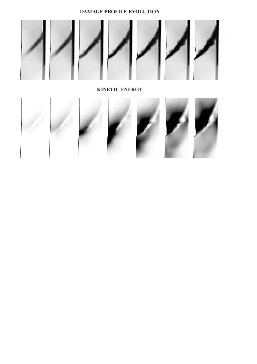
Figure 1: Simulations of a rupture in a two-dimensional specimen loaded by tension in a vertical direction, modelled by the phase-field crack approximation, and subsequent emission of an elastic wave. Seven selected snapshots are depicted. The decoupled energy-preserving time discretisation and P1-finite elements have been used.
                                                          Courtesy of Roman Vodička (Technical University Košice, Slovakia)

4.3 Explicit time discretisation outlined

Implicit schemes from Sect. 4.1 and 4.2 are not causal and not much efficient for real wave propagation calculations usually containing higher frequencies in comparison with mere vibrations. For this, more often, explicit schemes are used for real wave calculations, at least in linear elastodynamic models. These time-discretisation schemes work only if combined with space discretisation.

Disregarding damage and the viscous rheology, one efficient option often considered for waves in purely elastic materials is a so-called leapfrog scheme (also known as Verlet’s integration), i.e. central differences for the kinetic term

$$\mathscr{T}^{\prime}\frac{v_{\tau}^{k+1/2}-v_{\tau}^{k-1/2}}{\tau}+{\partial}_{u}\mathscr{E}_{h}(u_{\tau}^{k})=\mathscr{F}_{\tau}^{k}\ \ \ \ \text{ with }\ \ v_{\tau}^{k+1/2}=\frac{u_{\tau}^{k+1}{-}u_{\tau}^{k}}{\tau}.$$ (93)

The test by $v_{\tau}^{k+1/2}$ leads to a slightly twisted energy (im)balance:

$$\mathcal{T}\big{(}v_{\tau}^{k+1/2}\big{)}+\frac{1}{2}\big{\langle}{\partial}_{u}\mathscr{E}_{h}(u_{\tau}^{k}),u_{\tau}^{k+1}\big{\rangle}=\mathcal{T}\big{(}v_{\tau}^{k-1/2}\big{)}+\frac{1}{2}\big{\langle}{\partial}_{u}\mathscr{E}_{h}(u_{\tau}^{k-1}),u_{\tau}^{k}\big{\rangle}+\big{\langle}\mathscr{F}_{\tau}^{k},v_{\tau}^{k+1/2}\big{\rangle}.$$

This gives a correct kinetic energy but the stored energy is correct only asymptotically under the Courant-Friedrichs-Lewy (so-called CFL) condition [16], which needs also a space discretisation (here indicated by the abstract “mesh parameter” $h>0$) and the time step sufficiently small with respect to $h$; typically $\tau<Vh$ with $V$ the maximal speed of arising waves if $h$ has the meaning of a size of the largest element in a finite-element discretisation.

The option (93) does not seem directly amenable for being merged with the damage evolution. Another option relies on the reformulation of the elastodynamics in terms of velocity and stress, i.e. in terms of $v=\mathchoice{{\buildrel\hskip 1.00006pt\text{\LARGE.}\over{u}}}{{\buildrel\hskip 1.00006pt\text{\Large.}\over{u}}}{{\buildrel\hskip 1.00006pt\text{\large.}\over{u}}}{{\buildrel\hskip 1.00006pt\text{\large.}\over{u}}}$ and of the stress $\sigma:={\mathbb{C}}e(u)$, eliminating the displacement $u$. We thus have in mind the system

$$\mathchoice{{\buildrel\hskip 1.00006pt\text{\LARGE.}\over{\sigma}}}{{\buildrel\hskip 1.00006pt\text{\Large.}\over{\sigma}}}{{\buildrel\hskip 1.00006pt\text{\large.}\over{\sigma}}}{{\buildrel\hskip 1.00006pt\text{\large.}\over{\sigma}}}={\mathbb{C}}e(v)\ \ \ \text{ and }\ \ \ \varrho\mathchoice{{\buildrel\hskip 1.00006pt\text{\LARGE.}\over{v}}}{{\buildrel\hskip 1.00006pt\text{\Large.}\over{v}}}{{\buildrel\hskip 1.00006pt\text{\large.}\over{v}}}{{\buildrel\hskip 1.00006pt\text{\large.}\over{v}}}-{\rm div}\,\sigma=f \text{in }\ Q,$$ (94a)

$$\mathchoice{{\buildrel\hskip 1.00006pt\text{\LARGE.}\over{\sigma}}}{{\buildrel\hskip 1.00006pt\text{\Large.}\over{\sigma}}}{{\buildrel\hskip 1.00006pt\text{\large.}\over{\sigma}}}{{\buildrel\hskip 1.00006pt\text{\large.}\over{\sigma}}}\vec{n}=\mathchoice{{\buildrel\hskip 1.00006pt\text{\LARGE.}\over{g}}}{{\buildrel\hskip 1.00006pt\text{\Large.}\over{g}}}{{\buildrel\hskip 1.00006pt\text{\large.}\over{g}}}{{\buildrel\hskip 1.00006pt\text{\large.}\over{g}}} \text{on }\ \varSigma,$$ (94b)

$$v|_{t=0}=v_{0},\ \ \ \sigma|_{t=0}=\sigma_{0}:={\mathbb{C}}e(u_{0}) \text{{\color[rgb]{0,0,0}in} }\ \varOmega.$$ (94c)

The explicit staggered (called also “leap-frog”) time-discretisation can now be done as

$$\frac{\sigma_{\tau}^{k}-\sigma_{\tau}^{k-1}}{\tau}={\mathbb{C}}e(v_{\tau}^{k-1})\ \ \text{ and }\ \ \varrho\frac{v_{\tau}^{k}-v_{\tau}^{k-1}}{\tau}-{\rm div}\sigma_{\tau}^{k}=f_{\tau}^{k} \text{in }\ Q,$$ (95a)

$$\frac{\sigma_{\tau}^{k}-\sigma_{\tau}^{k-1}}{\tau}\vec{n}=\frac{g_{\tau}^{k}-g_{\tau}^{k-1}}{\tau} \text{on }\ \varSigma,$$ (95b)

$$v_{\tau}^{0}=v_{0},\ \ \ \sigma_{\tau}^{0}=\sigma_{0}:={\mathbb{C}}e(u_{0}) \text{{\color[rgb]{0,0,0}in} }\ \varOmega.$$ (95c)

Let us note that (95a) is decoupled, i.e. one is first to compute $\sigma_{\tau}^{k}$ and then $v_{\tau}^{k}$. Averaging the second equation in (95a) at level $k$ and $k{-}1$ and testing it $v_{\tau}^{k-1}$ while testing the first equation in (95a) by $(\sigma_{\tau h}^{k}+\sigma_{\tau h}^{k-1})/2$, we obtain the approximate energy balance as

$$\frac{1}{2}\big{\langle}\mathcal{T}^{\prime}v_{\tau}^{k},v_{\tau}^{k-1}\big{\rangle}+\varPhi_{h}(\sigma_{\tau}^{k})=\frac{1}{2}\big{\langle}\mathcal{T}^{\prime}v_{\tau}^{k-1},v_{\tau}^{k-2}\big{\rangle}+\varPhi_{h}(\sigma_{\tau}^{k-1})+\big{\langle}\mathscr{F}_{\tau}^{k},v_{\tau}^{k-1}\big{\rangle}\,,$$ (96)

with $\varPhi$ the stored energy expressed in terms of stress. Now the stored energy is correct while the kinetic energy needs the CFL-condition, cf. [5]. In contrast with (93), this option is more compatible with possible enhancement of the stored energy by internal parameters as e.g. damage.

Assuming ${\mathbb{C}}(\alpha)=\gamma(\alpha){\mathbb{C}}_{1}$ as in (64), we consider the energy $\varPhi=\varPhi(\varsigma,\alpha)$ with a “proto-stress” $\varsigma={\mathbb{C}}_{1}e(u)$ and with $\varPhi(\varsigma,\alpha)=\int_{\varOmega}\frac{1}{2}\gamma(\alpha){\mathbb{C}}_{1}^{-1}\varsigma{:}\varsigma-{\phi}(\alpha)+\frac{\kappa}{2}|\nabla\alpha|^{2}\,{\rm d}x$; for a general concept see [66] although, in damage mechanics, this proto-stress is also called an effective stress, having a specific mechanical meaning [59]. An important trick is that the proto-stress does not explicitly involve $\alpha$ and its time derivate does not lead to $\mathchoice{{\buildrel\hskip 1.00006pt\text{\LARGE.}\over{\alpha}}}{{\buildrel\hskip 1.00006pt\text{\Large.}\over{\alpha}}}{{\buildrel\hskip 1.00006pt\text{\large.}\over{\alpha}}}{{\buildrel\hskip 1.00006pt\text{\large.}\over{\alpha}}}$. The system (94) enhnaced by damage like (39b) then looks as

$$\mathchoice{{\buildrel\hskip 1.00006pt\text{\LARGE.}\over{\varsigma}}}{{\buildrel\hskip 1.00006pt\text{\Large.}\over{\varsigma}}}{{\buildrel\hskip 1.00006pt\text{\large.}\over{\varsigma}}}{{\buildrel\hskip 1.00006pt\text{\large.}\over{\varsigma}}}={\mathbb{C}}_{1}e(v)\ \ \ \text{ and }\ \ \ \varrho\mathchoice{{\buildrel\hskip 1.00006pt\text{\LARGE.}\over{v}}}{{\buildrel\hskip 1.00006pt\text{\Large.}\over{v}}}{{\buildrel\hskip 1.00006pt\text{\large.}\over{v}}}{{\buildrel\hskip 1.00006pt\text{\large.}\over{v}}}-{\rm div}\,\sigma=f\ \ \ \text{ with }\ \ \ \sigma=\gamma(\alpha)\varsigma \text{in }\ Q,$$ (97a)

$${\partial}\zeta(\mathchoice{{\buildrel\hskip 1.00006pt\text{\LARGE.}\over{\alpha}}}{{\buildrel\hskip 1.00006pt\text{\Large.}\over{\alpha}}}{{\buildrel\hskip 1.00006pt\text{\large.}\over{\alpha}}}{{\buildrel\hskip 1.00006pt\text{\large.}\over{\alpha}}})+\frac{1}{2}\gamma^{\prime}(\alpha){\mathbb{C}}_{1}^{-1}\varsigma{:}\varsigma-{\rm div}\big{(}\kappa\nabla\alpha\big{)}\ni{\phi^{\prime}}(\alpha) \text{in }\ Q,$$ (97b)

$$\mathchoice{{\buildrel\hskip 1.00006pt\text{\LARGE.}\over{\sigma}}}{{\buildrel\hskip 1.00006pt\text{\Large.}\over{\sigma}}}{{\buildrel\hskip 1.00006pt\text{\large.}\over{\sigma}}}{{\buildrel\hskip 1.00006pt\text{\large.}\over{\sigma}}}\vec{n}=\mathchoice{{\buildrel\hskip 1.00006pt\text{\LARGE.}\over{g}}}{{\buildrel\hskip 1.00006pt\text{\Large.}\over{g}}}{{\buildrel\hskip 1.00006pt\text{\large.}\over{g}}}{{\buildrel\hskip 1.00006pt\text{\large.}\over{g}}}\ \ \text{ and }\ \ \kappa\nabla\alpha\cdot\vec{n}=0 \text{on }\ \varSigma,$$ (97c)

$$v|_{t=0}=v_{0},\ \ \ \sigma|_{t=0}=\sigma_{0}:={\mathbb{C}}e(u_{0}),\ \ \ \alpha|_{t=0}=\alpha_{0} \text{{\color[rgb]{0,0,0}in} }\ \varOmega.$$ (97d)

Applying the staggered discretisation like in Sect. 4.2, we obtain a 3-step scheme:

$$\frac{\varsigma_{\tau}^{k}-\varsigma_{\tau}^{k-1}}{\tau}={\mathbb{C}}_{1}e(v_{\tau}^{k-1}) \text{in }\ Q\,,$$ (98a)

$${\partial}\zeta\Big{(}\frac{\alpha_{\tau}^{k}-\alpha_{\tau}^{k-1}}{\tau}\Big{)}+\frac{1}{2}\gamma^{\circ}(\alpha_{\tau}^{k},\alpha_{\tau}^{k-1}){\mathbb{C}}_{1}^{-1}\varsigma_{\tau}^{k}{\colon}\varsigma_{\tau}^{k}-{\rm div}(\kappa\nabla\alpha_{\tau}^{k-1/2})\ni{\phi}^{\circ}(\alpha_{\tau}^{k},\alpha_{\tau}^{k-1}) \text{in }\ Q\,,$$ (98b)

$$\varrho\frac{v_{\tau}^{k}-v_{\tau}^{k-1}}{\tau}-{\rm div}\sigma_{\tau}^{k}=f_{\tau}^{k}\ \ \ \text{ with }\ \ \ \sigma_{\tau}^{k}=\gamma(\alpha_{\tau}^{k})\varsigma_{\tau}^{k} \text{in }\ Q\,,$$ (98c)

to be completed by the respective boundary conditions.

The analysis of (98) is however rather nontrivial and the analog of (96) with the corresponding damage terms like in (83) contains still some other term vanishing in the limit under the CFL condition, cf. [66] for details. Even more, as there is no Kelvin-Voigt viscosity which would be troublesome for such explicit discretisation, one needs still some higher-order gradient term not subject to damage and acting on $\varsigma$ to guarantee convergence of such a scheme; cf. also [37, Sect.7.5.3].

To conclude, it should be mentioned that a really efficient (i.e. explicit) numerical scheme with granted stability and convergence for the simple inviscid or viscous material undergoing damage does not seem to be devised so far.

5 Concluding remarks – some modifications

Many other phenomena can be combined with the plain damage in the Kelvin-Voigt vicoelastic model considered so far. Typically one can think about more complicated viscoelastic rheologies, involving possibly some inelastic processes as plasticity, which will be in a simple variant in Sect. 5.1.

Also, some diffusant (like water in poroelastic rocks or hydrogen in metals or some solvent in polymers) can propagate through the bulk by a Fick/Darcy law, interacting with mechanical properties including fracture toughness. Of course, full thermodynamical context should involve heat production and transfer through the Fourier law. Here we only refer to [63] where a staggered energy-conserving time discretisation like in Sect. 4.2 is devised. Damage with plasticity accompanied by heat production and heat transfer allows for fitting to the popular rate-and-state-dependent friction model [62].

Moreover, the plain models from Sections 2–3 together with all these extensions can be considered within the large strains, too. We will outline it Sect. 5.2.

5.1 Combination with creep or plasticity

The Kelvin-Voigt rheology is mathematically the most basic viscoelastic rheology of parabolic type. In particular from the wave-propagation viewpoint, physically more natural is that Maxwell rheology but it is rather hyperbolic and mathematically troublesome if accompanied with inelastic processes like damage. A certain reasonable compromise it the Jeffreys’ rheology combining the Norton-Hoff (also called Stokes) and Kelvin-Voigt rheology in series (or alternatively Maxwell’s and Norton-Hoff’s rheology in parallel). It can capture creep effects, which have sense in the shear part rather than the spherical part.

Instead (or in addition) to the linear Norton-Hoff dumper in the shear part, one can consider also the activated plastic element. The schematic rheological model is depicted in Figure 2, distinguishing also the compression and the tension in the spherical part.

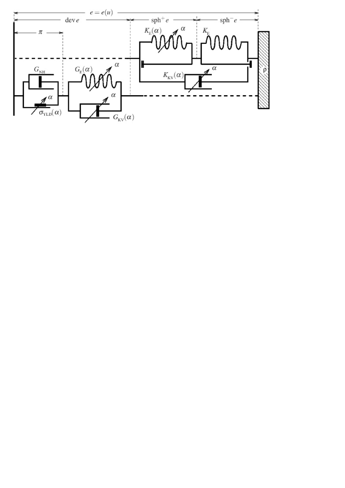
Figure 2: Schematic diagram for the viscoelastic Jeffreys rheology (if $\sigma_{\text{\sc yld}}=0$) which is subjected to damage $\alpha$ in the deviatoric part except undamageable creep (the $G_{{}_{\rm NH}}$-dashpot) while the Kelvin-Voigt rheology in the spherical (volumetric) part is subjected to damage only under tension but not compression. For $\sigma_{\text{\sc yld}}>0$, it models (visco)plasticity. Evolution of damage is not depicted.

The additional dissipation due to isochoric plastification is then achieved when damage is performed in a shear mode (i.e. Mode II) comparing to damage by opening (i.e. Mode I) where plastification is not triggered. When considering the isotropic stored energy (54a) with damage without any hardening-like effects (i.e. linearly-depending $K_{{}_{\rm E}}(\alpha)=\alpha K$ and $G_{{}_{\rm E}}(\alpha)=\alpha G$) and with ${\phi}(\alpha)$ also linear and the elastic strain $e-\pi$ in place of the total strain $e$ combined with the isotropic hardening with $\sigma_{\text{\tiny{DAM}}}=0$, we altogether arrive at the model governed by

$$\varphi_{\text{\sc e}}(e,\alpha,\pi,\nabla\alpha,\nabla\pi)=\frac{d}{2}\Big{(}K_{{}_{\rm E}}|{\rm sph}^{-}e|^{2}+K_{{}_{\rm E}}(\alpha)|{\rm sph}^{+}e|^{2}\Big{)}+G_{{}_{\rm E}}(\alpha)|{\rm dev}e{-}\pi|^{2}$$

$$\qquad\qquad\qquad\qquad\qquad\quad-{\phi^{\prime}}(\alpha)+\frac{1}{2}H|\pi|^{2}+\frac{\kappa_{1}}{2}|\nabla\pi|^{2}+\frac{\kappa_{2}}{2}|\nabla\alpha|^{2},$$ (99a)

$$\zeta(\alpha;\mathchoice{{\buildrel\hskip 1.00006pt\text{\LARGE.}\over{e}}}{{\buildrel\hskip 1.00006pt\text{\Large.}\over{e}}}{{\buildrel\hskip 1.00006pt\text{\large.}\over{e}}}{{\buildrel\hskip 1.00006pt\text{\large.}\over{e}}},\mathchoice{{\buildrel\hskip 1.00006pt\text{\LARGE.}\over{\alpha}}}{{\buildrel\hskip 1.00006pt\text{\Large.}\over{\alpha}}}{{\buildrel\hskip 1.00006pt\text{\large.}\over{\alpha}}}{{\buildrel\hskip 1.00006pt\text{\large.}\over{\alpha}}},\mathchoice{{\buildrel\hskip 1.00006pt\text{\LARGE.}\over{\pi}}}{{\buildrel\hskip 1.00006pt\text{\Large.}\over{\pi}}}{{\buildrel\hskip 1.00006pt\text{\large.}\over{\pi}}}{{\buildrel\hskip 1.00006pt\text{\large.}\over{\pi}}})=\frac{d}{2}K_{\text{\sc kv}}(\alpha)|{\rm sph}\,\mathchoice{{\buildrel\hskip 1.00006pt\text{\LARGE.}\over{e}}}{{\buildrel\hskip 1.00006pt\text{\Large.}\over{e}}}{{\buildrel\hskip 1.00006pt\text{\large.}\over{e}}}{{\buildrel\hskip 1.00006pt\text{\large.}\over{e}}}|^{2}+G_{\text{\sc kv}}(\alpha)|{\rm dev}\mathchoice{{\buildrel\hskip 1.00006pt\text{\LARGE.}\over{e}}}{{\buildrel\hskip 1.00006pt\text{\Large.}\over{e}}}{{\buildrel\hskip 1.00006pt\text{\large.}\over{e}}}{{\buildrel\hskip 1.00006pt\text{\large.}\over{e}}}{-}\mathchoice{{\buildrel\hskip 1.00006pt\text{\LARGE.}\over{\pi}}}{{\buildrel\hskip 1.00006pt\text{\Large.}\over{\pi}}}{{\buildrel\hskip 1.00006pt\text{\large.}\over{\pi}}}{{\buildrel\hskip 1.00006pt\text{\large.}\over{\pi}}}|^{2}+\frac{1}{2}G_{\text{\sc nh}}|\mathchoice{{\buildrel\hskip 1.00006pt\text{\LARGE.}\over{\pi}}}{{\buildrel\hskip 1.00006pt\text{\Large.}\over{\pi}}}{{\buildrel\hskip 1.00006pt\text{\large.}\over{\pi}}}{{\buildrel\hskip 1.00006pt\text{\large.}\over{\pi}}}|^{2}+\sigma_{\text{\sc yld}}(\alpha)|\mathchoice{{\buildrel\hskip 1.00006pt\text{\LARGE.}\over{\pi}}}{{\buildrel\hskip 1.00006pt\text{\Large.}\over{\pi}}}{{\buildrel\hskip 1.00006pt\text{\large.}\over{\pi}}}{{\buildrel\hskip 1.00006pt\text{\large.}\over{\pi}}}|+\delta_{[0,+\infty)}^{*}(\mathchoice{{\buildrel\hskip 1.00006pt\text{\LARGE.}\over{\alpha}}}{{\buildrel\hskip 1.00006pt\text{\Large.}\over{\alpha}}}{{\buildrel\hskip 1.00006pt\text{\large.}\over{\alpha}}}{{\buildrel\hskip 1.00006pt\text{\large.}\over{\alpha}}})+\frac{\nu}{2}\mathchoice{{\buildrel\hskip 1.00006pt\text{\LARGE.}\over{\alpha}}}{{\buildrel\hskip 1.00006pt\text{\Large.}\over{\alpha}}}{{\buildrel\hskip 1.00006pt\text{\large.}\over{\alpha}}}{{\buildrel\hskip 1.00006pt\text{\large.}\over{\alpha}}}^{2},$$ (99b)

where the specific dissipation potential now contains another damper $G_{\text{\sc nh}}$ which facilitates to the Jeffrey’s model in the shear part and a yield stress $\sigma_{\text{\sc yld}}{}\geq 0$ possibly depending on damage, which can model activated inelastic plastic response. Starting from undamaged material, the energy needed (dissipated) by damaging in opening without plastification is just the toughness ${\mathfrak{g}}_{\rm c}:={\phi}^{\prime}(1)$, while in shearing mode it is larger, namely ${\mathfrak{g}}_{\rm c}+\sigma_{\text{\sc yld}}(\sqrt{2G{\mathfrak{g}}_{\rm c}}-\sigma_{\text{\sc yld}})/H$ provided the parameters are tuned in a way to satisfy $\sqrt{G{\mathfrak{g}}_{\rm c}/2}<\sigma_{\text{\sc yld}}\leq\sqrt{2G{\mathfrak{g}}_{\rm c}}$. This was first devised for an interfacial delamination model [68], being inspired just by such bulk plasticity.

Let us illustrate the staggered scheme (81) in the case of a linearly responding material, i.e. $K_{{}_{\rm E}}|{\rm sph}^{-}e|^{2}+K_{{}_{\rm E}}(\alpha)|{\rm sph}^{+}e|^{2}$ is simplied to $K_{{}_{\rm E}}(\alpha)|{\rm sph}\,e|^{2}$ in (99a), denoting ${\mathbb{C}}_{ijkl}(\alpha)=K_{\text{\sc e}}(\alpha)\delta_{ij}\delta_{kl}+G_{\text{\sc e}}(\alpha)(\delta_{ik}\delta_{jl}+\delta_{il}\delta_{jk}-\frac{2}{d}\delta_{ij}\delta_{kl})$ and ${\mathbb{D}}_{ijkl}(\alpha)=K_{\text{\sc kv}}(\alpha)\delta_{ij}\delta_{kl}+G_{\text{\sc kv}}(\alpha)(\delta_{ik}\delta_{jl}+\delta_{il}\delta_{jk}-\frac{2}{d}\delta_{ij}\delta_{kl})$ with $\delta$ standing for the Kronecker symbol. More specifically, introducing a notation for the elastic strain $e_{\rm el}=e(u){-}\pi$ and its discretisation $e_{\rm el,\tau}=e(u_{\tau}){-}\pi_{\tau}$ and $\underline{\overline{e}}_{\rm el,\tau}=e(\underline{\overline{u}}_{\tau}){-}\underline{\overline{\pi}}_{\tau}$, the system (81) can be expanded as

$$\mathchoice{{\buildrel\hskip 1.00006pt\text{\LARGE.}\over{u}}}{{\buildrel\hskip 1.00006pt\text{\Large.}\over{u}}}{{\buildrel\hskip 1.00006pt\text{\large.}\over{u}}}{{\buildrel\hskip 1.00006pt\text{\large.}\over{u}}}_{\tau}=\underline{\overline{v}}_{\tau}\ \ \ \ \ \text{ and }\ \ \ \ \ \varrho\mathchoice{{\buildrel\hskip 1.00006pt\text{\LARGE.}\over{v}}}{{\buildrel\hskip 1.00006pt\text{\Large.}\over{v}}}{{\buildrel\hskip 1.00006pt\text{\large.}\over{v}}}{{\buildrel\hskip 1.00006pt\text{\large.}\over{v}}}_{\tau}-{\rm div}\big{(}{\mathbb{D}}(\hskip 1.00006pt\underline{\alpha}_{\tau})\mathchoice{{\buildrel\hskip 1.00006pt\text{\LARGE.}\over{e}}}{{\buildrel\hskip 1.00006pt\text{\Large.}\over{e}}}{{\buildrel\hskip 1.00006pt\text{\large.}\over{e}}}{{\buildrel\hskip 1.00006pt\text{\large.}\over{e}}}_{\rm el,\tau}+{\mathbb{C}}(\hskip 1.00006pt\underline{\alpha}_{\tau})\underline{\overline{e}}_{\rm el,\tau}\big{)}=\overline{f}_{\tau}\,,$$ (100a)

$$\sigma_{\text{\sc yld}}(\hskip 1.00006pt\underline{\alpha}_{\tau}){\rm Dir}(\mathchoice{{\buildrel\hskip 1.00006pt\text{\LARGE.}\over{\pi}}}{{\buildrel\hskip 1.00006pt\text{\Large.}\over{\pi}}}{{\buildrel\hskip 1.00006pt\text{\large.}\over{\pi}}}{{\buildrel\hskip 1.00006pt\text{\large.}\over{\pi}}}_{\tau})+H\underline{\overline{\pi}}_{\tau}-{\rm div}(\kappa_{1}\nabla\underline{\overline{\pi}}_{\tau})\ni{\rm dev}\big{(}{\mathbb{D}}(\hskip 1.00006pt\underline{\alpha}_{\tau})\mathchoice{{\buildrel\hskip 1.00006pt\text{\LARGE.}\over{e}}}{{\buildrel\hskip 1.00006pt\text{\Large.}\over{e}}}{{\buildrel\hskip 1.00006pt\text{\large.}\over{e}}}{{\buildrel\hskip 1.00006pt\text{\large.}\over{e}}}_{\rm el,\tau}+{\mathbb{C}}(\hskip 1.00006pt\underline{\alpha}_{\tau})\underline{\overline{e}}_{\rm el,\tau}\big{)},$$ (100b)

$${\partial}\zeta\big{(}\mathchoice{{\buildrel\hskip 1.00006pt\text{\LARGE.}\over{\alpha}}}{{\buildrel\hskip 1.00006pt\text{\Large.}\over{\alpha}}}{{\buildrel\hskip 1.00006pt\text{\large.}\over{\alpha}}}{{\buildrel\hskip 1.00006pt\text{\large.}\over{\alpha}}}_{\tau}\big{)}+\frac{1}{2}{\mathbb{C}}^{\circ}(\hskip 1.00006pt\overline{\alpha}_{\tau},\hskip 1.00006pt\underline{\alpha}_{\tau})\overline{e}_{\rm el,\tau}{\colon}\overline{e}_{\rm el,\tau}-{\rm div}(\kappa_{2}\nabla\underline{\hskip 1.00006pt\overline{\alpha}}_{\tau})\ni{\phi}^{\circ}(\hskip 1.00006pt\overline{\alpha}_{\tau},\hskip 1.00006pt\underline{\alpha}_{\tau})\,.$$ (100c)

The boundary conditions can be written analogously. Now, the splitting during the recursive time-stepping procedure concerns separately (100a,b) and (100c), both these boundary-value problems at particular time levels having a potential. The basic energy estimates can be obtained by testing the particular equations/inclusions in (100) subsequently by $v_{\tau}$, $\mathchoice{{\buildrel\hskip 1.00006pt\text{\LARGE.}\over{\pi}}}{{\buildrel\hskip 1.00006pt\text{\Large.}\over{\pi}}}{{\buildrel\hskip 1.00006pt\text{\large.}\over{\pi}}}{{\buildrel\hskip 1.00006pt\text{\large.}\over{\pi}}}_{\tau}$, and $\mathchoice{{\buildrel\hskip 1.00006pt\text{\LARGE.}\over{\alpha}}}{{\buildrel\hskip 1.00006pt\text{\Large.}\over{\alpha}}}{{\buildrel\hskip 1.00006pt\text{\large.}\over{\alpha}}}{{\buildrel\hskip 1.00006pt\text{\large.}\over{\alpha}}}_{\tau}$, using the quadratic trick several times (e.g. for $\varrho\mathchoice{{\buildrel\hskip 1.00006pt\text{\LARGE.}\over{v}}}{{\buildrel\hskip 1.00006pt\text{\Large.}\over{v}}}{{\buildrel\hskip 1.00006pt\text{\large.}\over{v}}}{{\buildrel\hskip 1.00006pt\text{\large.}\over{v}}}_{\tau}\cdot\underline{\overline{v}}_{\tau}=\frac{\partial}{\partial t}\frac{1}{2}|\underline{\overline{v}}_{\tau}|^{2}$ a.e. o $Q$) and the cancellation of the terms $\pm{\mathbb{C}}(\hskip 1.00006pt\underline{\alpha}_{\tau})\overline{e}_{\rm el,\tau}{\colon}\overline{e}_{\rm el,\tau}$ arising by these tests.

For the strong convergence of $\overline{e}_{\rm el,\tau}$, instead of the strategies (44) or (47), we now rely rather on the test of (100a,b) respectively by $\mathchoice{{\buildrel\hskip 1.00006pt\text{\LARGE.}\over{u}}}{{\buildrel\hskip 1.00006pt\text{\Large.}\over{u}}}{{\buildrel\hskip 1.00006pt\text{\large.}\over{u}}}{{\buildrel\hskip 1.00006pt\text{\large.}\over{u}}}_{\tau}{-}\mathchoice{{\buildrel\hskip 1.00006pt\text{\LARGE.}\over{u}}}{{\buildrel\hskip 1.00006pt\text{\Large.}\over{u}}}{{\buildrel\hskip 1.00006pt\text{\large.}\over{u}}}{{\buildrel\hskip 1.00006pt\text{\large.}\over{u}}}$ and $\mathchoice{{\buildrel\hskip 1.00006pt\text{\LARGE.}\over{\pi}}}{{\buildrel\hskip 1.00006pt\text{\Large.}\over{\pi}}}{{\buildrel\hskip 1.00006pt\text{\large.}\over{\pi}}}{{\buildrel\hskip 1.00006pt\text{\large.}\over{\pi}}}_{\tau}{-}\mathchoice{{\buildrel\hskip 1.00006pt\text{\LARGE.}\over{\pi}}}{{\buildrel\hskip 1.00006pt\text{\Large.}\over{\pi}}}{{\buildrel\hskip 1.00006pt\text{\large.}\over{\pi}}}{{\buildrel\hskip 1.00006pt\text{\large.}\over{\pi}}}$. We need ${\mathbb{C}}$ monotone (nondecreasing) with respect to the Löwner ordering, and we use the unidirectionality of the damage evolution, i.e. $\mathchoice{{\buildrel\hskip 1.00006pt\text{\LARGE.}\over{\alpha}}}{{\buildrel\hskip 1.00006pt\text{\Large.}\over{\alpha}}}{{\buildrel\hskip 1.00006pt\text{\large.}\over{\alpha}}}{{\buildrel\hskip 1.00006pt\text{\large.}\over{\alpha}}}_{\tau}\leq 0$. We first approximate the limit $u$ and $\pi$, defining $\widetilde{u}_{\tau}^{k}:={\color[rgb]{0,0,0}\frac{1}{\tau}}\int_{(k-1)\tau}^{k\tau}u(t)\,{\rm d}t$ and $\widetilde{\pi}_{\tau}^{k}:={\color[rgb]{0,0,0}\frac{1}{\tau}}\int_{(k-1)\tau}^{k\tau}\pi(t)\,{\rm d}t$, and then put $\varepsilon_{\rm el,\tau}^{k}:=e(\widetilde{u}_{\tau}^{k})-\widetilde{\pi}_{\tau}^{k}$. Then also the interpolants $\varepsilon_{\rm el,\tau}$ and $\underline{\overline{\varepsilon}}_{\rm el,\tau}$ which both converges to $e_{\rm el}$ strongly. This approximation allows us to estimate

$$\frac{1}{2}{\mathbb{C}}(\alpha_{\tau}(T))(e_{\rm el,\tau}(T)-\varepsilon_{\rm el,\tau}(T)){\colon}(e_{\rm el,\tau}(T)-\varepsilon_{\rm el,\tau}(T))$$

$$\ =\int_{0}^{T}\Big{(}{\mathbb{C}}(\hskip 1.00006pt\underline{\alpha}_{\tau})(\underline{\overline{e}}_{\rm el,\tau}{-}\underline{\overline{\varepsilon}}_{\rm el,\tau}){\colon}(\mathchoice{{\buildrel\hskip 1.00006pt\text{\LARGE.}\over{e}}}{{\buildrel\hskip 1.00006pt\text{\Large.}\over{e}}}{{\buildrel\hskip 1.00006pt\text{\large.}\over{e}}}{{\buildrel\hskip 1.00006pt\text{\large.}\over{e}}}_{\rm el,\tau}{-}\mathchoice{{\buildrel\hskip 1.00006pt\text{\LARGE.}\over{\varepsilon}}}{{\buildrel\hskip 1.00006pt\text{\Large.}\over{\varepsilon}}}{{\buildrel\hskip 1.00006pt\text{\large.}\over{\varepsilon}}}{{\buildrel\hskip 1.00006pt\text{\large.}\over{\varepsilon}}}_{\rm el,\tau})-\frac{1}{2}\mathchoice{{\buildrel\hskip 1.00006pt\text{\LARGE.}\over{\alpha}}}{{\buildrel\hskip 1.00006pt\text{\Large.}\over{\alpha}}}{{\buildrel\hskip 1.00006pt\text{\large.}\over{\alpha}}}{{\buildrel\hskip 1.00006pt\text{\large.}\over{\alpha}}}_{\tau}{\mathbb{C}}^{\circ}(\hskip 1.00006pt\overline{\alpha}_{\tau},\hskip 1.00006pt\underline{\alpha}_{\tau})(\underline{\overline{e}}_{\rm el,\tau}{-}\underline{\overline{\varepsilon}}_{\rm el,\tau}){\colon}$$

$$\qquad\qquad\qquad{\colon}(\underline{\overline{e}}_{\rm el,\tau}{-}\underline{\overline{\varepsilon}}_{\rm el,\tau})\Big{)}\,{\rm d}t\geq\int_{0}^{T}{\mathbb{C}}(\hskip 1.00006pt\underline{\alpha}_{\tau})(\underline{\overline{e}}_{\rm el,\tau}{-}\underline{\overline{\varepsilon}}_{\rm el,\tau}){\colon}(\mathchoice{{\buildrel\hskip 1.00006pt\text{\LARGE.}\over{e}}}{{\buildrel\hskip 1.00006pt\text{\Large.}\over{e}}}{{\buildrel\hskip 1.00006pt\text{\large.}\over{e}}}{{\buildrel\hskip 1.00006pt\text{\large.}\over{e}}}_{\rm el,\tau}{-}\mathchoice{{\buildrel\hskip 1.00006pt\text{\LARGE.}\over{\varepsilon}}}{{\buildrel\hskip 1.00006pt\text{\Large.}\over{\varepsilon}}}{{\buildrel\hskip 1.00006pt\text{\large.}\over{\varepsilon}}}{{\buildrel\hskip 1.00006pt\text{\large.}\over{\varepsilon}}}_{\rm el,\tau})\,{\rm d}t$$

a.e. on $\Omega$. When integrate over $\Omega$, this allows us to estimate:

$$\int_{\Omega}\frac{1}{2}{\mathbb{C}}(\alpha_{\tau}(T))(e_{\rm el,\tau}(T)-\varepsilon_{\rm el,\tau}(T)){\colon}(e_{\rm el,\tau}(T)-\varepsilon_{\rm el,\tau}(T))\,{\rm d}x+\int_{Q}{\mathbb{D}}(\hskip 1.00006pt\underline{\alpha}_{\tau})(\mathchoice{{\buildrel\hskip 1.00006pt\text{\LARGE.}\over{e}}}{{\buildrel\hskip 1.00006pt\text{\Large.}\over{e}}}{{\buildrel\hskip 1.00006pt\text{\large.}\over{e}}}{{\buildrel\hskip 1.00006pt\text{\large.}\over{e}}}_{\rm el,\tau}{-}\mathchoice{{\buildrel\hskip 1.00006pt\text{\LARGE.}\over{\varepsilon}}}{{\buildrel\hskip 1.00006pt\text{\Large.}\over{\varepsilon}}}{{\buildrel\hskip 1.00006pt\text{\large.}\over{\varepsilon}}}{{\buildrel\hskip 1.00006pt\text{\large.}\over{\varepsilon}}}_{\rm el,\tau}){\colon}(\mathchoice{{\buildrel\hskip 1.00006pt\text{\LARGE.}\over{e}}}{{\buildrel\hskip 1.00006pt\text{\Large.}\over{e}}}{{\buildrel\hskip 1.00006pt\text{\large.}\over{e}}}{{\buildrel\hskip 1.00006pt\text{\large.}\over{e}}}_{\rm el,\tau}{-}\mathchoice{{\buildrel\hskip 1.00006pt\text{\LARGE.}\over{\varepsilon}}}{{\buildrel\hskip 1.00006pt\text{\Large.}\over{\varepsilon}}}{{\buildrel\hskip 1.00006pt\text{\large.}\over{\varepsilon}}}{{\buildrel\hskip 1.00006pt\text{\large.}\over{\varepsilon}}}_{\rm el,\tau})\,{\rm d}x{\rm d}t$$

$$\quad\leq\int_{Q}\Big{(}{\mathbb{D}}(\hskip 1.00006pt\underline{\alpha}_{\tau})(\mathchoice{{\buildrel\hskip 1.00006pt\text{\LARGE.}\over{e}}}{{\buildrel\hskip 1.00006pt\text{\Large.}\over{e}}}{{\buildrel\hskip 1.00006pt\text{\large.}\over{e}}}{{\buildrel\hskip 1.00006pt\text{\large.}\over{e}}}_{\rm el,\tau}{-}\mathchoice{{\buildrel\hskip 1.00006pt\text{\LARGE.}\over{\varepsilon}}}{{\buildrel\hskip 1.00006pt\text{\Large.}\over{\varepsilon}}}{{\buildrel\hskip 1.00006pt\text{\large.}\over{\varepsilon}}}{{\buildrel\hskip 1.00006pt\text{\large.}\over{\varepsilon}}}_{\rm el,\tau})+{\mathbb{C}}(\hskip 1.00006pt\underline{\alpha}_{\tau})(\underline{\overline{e}}_{\rm el,\tau}{-}\underline{\overline{\varepsilon}}_{\rm el,\tau})\Big{)}{\colon}(\mathchoice{{\buildrel\hskip 1.00006pt\text{\LARGE.}\over{e}}}{{\buildrel\hskip 1.00006pt\text{\Large.}\over{e}}}{{\buildrel\hskip 1.00006pt\text{\large.}\over{e}}}{{\buildrel\hskip 1.00006pt\text{\large.}\over{e}}}_{\rm el,\tau}{-}\mathchoice{{\buildrel\hskip 1.00006pt\text{\LARGE.}\over{\varepsilon}}}{{\buildrel\hskip 1.00006pt\text{\Large.}\over{\varepsilon}}}{{\buildrel\hskip 1.00006pt\text{\large.}\over{\varepsilon}}}{{\buildrel\hskip 1.00006pt\text{\large.}\over{\varepsilon}}}_{\rm el,\tau})\,{\rm d}x{\rm d}t$$

$$\quad=\int_{Q}(\overline{f}_{\tau}-\varrho\mathchoice{{\buildrel\hskip 1.00006pt\text{\LARGE.}\over{v}}}{{\buildrel\hskip 1.00006pt\text{\Large.}\over{v}}}{{\buildrel\hskip 1.00006pt\text{\large.}\over{v}}}{{\buildrel\hskip 1.00006pt\text{\large.}\over{v}}}_{\tau})\!\cdot\!(\underline{\overline{v}}_{\tau}{-}\mathchoice{{\buildrel\hskip 1.00006pt\text{\LARGE.}\over{\widetilde{u}}}}{{\buildrel\hskip 1.00006pt\text{\Large.}\over{\widetilde{u}}}}{{\buildrel\hskip 1.00006pt\text{\large.}\over{\widetilde{u}}}}{{\buildrel\hskip 1.00006pt\text{\large.}\over{\widetilde{u}}}}_{\tau})-\Big{(}{\mathbb{D}}(\hskip 1.00006pt\underline{\alpha}_{\tau})\mathchoice{{\buildrel\hskip 1.00006pt\text{\LARGE.}\over{\varepsilon}}}{{\buildrel\hskip 1.00006pt\text{\Large.}\over{\varepsilon}}}{{\buildrel\hskip 1.00006pt\text{\large.}\over{\varepsilon}}}{{\buildrel\hskip 1.00006pt\text{\large.}\over{\varepsilon}}}_{\rm el,\tau}+{\mathbb{C}}(\hskip 1.00006pt\underline{\alpha}_{\tau})\underline{\overline{\varepsilon}}_{\rm el,\tau}\Big{)}{\colon}(\mathchoice{{\buildrel\hskip 1.00006pt\text{\LARGE.}\over{e}}}{{\buildrel\hskip 1.00006pt\text{\Large.}\over{e}}}{{\buildrel\hskip 1.00006pt\text{\large.}\over{e}}}{{\buildrel\hskip 1.00006pt\text{\large.}\over{e}}}_{\rm el,\tau}{-}\mathchoice{{\buildrel\hskip 1.00006pt\text{\LARGE.}\over{\varepsilon}}}{{\buildrel\hskip 1.00006pt\text{\Large.}\over{\varepsilon}}}{{\buildrel\hskip 1.00006pt\text{\large.}\over{\varepsilon}}}{{\buildrel\hskip 1.00006pt\text{\large.}\over{\varepsilon}}}_{\rm el,\tau})$$

$$\qquad\ +\sigma_{\text{\sc yld}}(\alpha_{\tau})(|\mathchoice{{\buildrel\hskip 1.00006pt\text{\LARGE.}\over{\pi}}}{{\buildrel\hskip 1.00006pt\text{\Large.}\over{\pi}}}{{\buildrel\hskip 1.00006pt\text{\large.}\over{\pi}}}{{\buildrel\hskip 1.00006pt\text{\large.}\over{\pi}}}|-|\mathchoice{{\buildrel\hskip 1.00006pt\text{\LARGE.}\over{\pi}}}{{\buildrel\hskip 1.00006pt\text{\Large.}\over{\pi}}}{{\buildrel\hskip 1.00006pt\text{\large.}\over{\pi}}}{{\buildrel\hskip 1.00006pt\text{\large.}\over{\pi}}}_{\tau}|)+H\underline{\overline{\pi}}_{\tau}{\colon}(\mathchoice{{\buildrel\hskip 1.00006pt\text{\LARGE.}\over{\pi}}}{{\buildrel\hskip 1.00006pt\text{\Large.}\over{\pi}}}{{\buildrel\hskip 1.00006pt\text{\large.}\over{\pi}}}{{\buildrel\hskip 1.00006pt\text{\large.}\over{\pi}}}-\mathchoice{{\buildrel\hskip 1.00006pt\text{\LARGE.}\over{\pi}}}{{\buildrel\hskip 1.00006pt\text{\Large.}\over{\pi}}}{{\buildrel\hskip 1.00006pt\text{\large.}\over{\pi}}}{{\buildrel\hskip 1.00006pt\text{\large.}\over{\pi}}}_{\tau})+\kappa_{1}\nabla\underline{\overline{\pi}}_{\tau}{\vdots}\nabla(\mathchoice{{\buildrel\hskip 1.00006pt\text{\LARGE.}\over{\pi}}}{{\buildrel\hskip 1.00006pt\text{\Large.}\over{\pi}}}{{\buildrel\hskip 1.00006pt\text{\large.}\over{\pi}}}{{\buildrel\hskip 1.00006pt\text{\large.}\over{\pi}}}-\mathchoice{{\buildrel\hskip 1.00006pt\text{\LARGE.}\over{\pi}}}{{\buildrel\hskip 1.00006pt\text{\Large.}\over{\pi}}}{{\buildrel\hskip 1.00006pt\text{\large.}\over{\pi}}}{{\buildrel\hskip 1.00006pt\text{\large.}\over{\pi}}}_{\tau})\to 0$$ (101)

From this $\mathchoice{{\buildrel\hskip 1.00006pt\text{\LARGE.}\over{e}}}{{\buildrel\hskip 1.00006pt\text{\Large.}\over{e}}}{{\buildrel\hskip 1.00006pt\text{\large.}\over{e}}}{{\buildrel\hskip 1.00006pt\text{\large.}\over{e}}}_{\rm el,\tau}{-}\mathchoice{{\buildrel\hskip 1.00006pt\text{\LARGE.}\over{\varepsilon}}}{{\buildrel\hskip 1.00006pt\text{\Large.}\over{\varepsilon}}}{{\buildrel\hskip 1.00006pt\text{\large.}\over{\varepsilon}}}{{\buildrel\hskip 1.00006pt\text{\large.}\over{\varepsilon}}}_{\rm el,\tau}\to 0$ strongly in $L^{2}(Q;{\mathbb{R}}^{d\times d}_{\rm sym})$. Since $\mathchoice{{\buildrel\hskip 1.00006pt\text{\LARGE.}\over{\varepsilon}}}{{\buildrel\hskip 1.00006pt\text{\Large.}\over{\varepsilon}}}{{\buildrel\hskip 1.00006pt\text{\large.}\over{\varepsilon}}}{{\buildrel\hskip 1.00006pt\text{\large.}\over{\varepsilon}}}_{\rm el,\tau}\to\mathchoice{{\buildrel\hskip 1.00006pt\text{\LARGE.}\over{e}}}{{\buildrel\hskip 1.00006pt\text{\Large.}\over{e}}}{{\buildrel\hskip 1.00006pt\text{\large.}\over{e}}}{{\buildrel\hskip 1.00006pt\text{\large.}\over{e}}}_{\rm el}$, we obtain $\mathchoice{{\buildrel\hskip 1.00006pt\text{\LARGE.}\over{e}}}{{\buildrel\hskip 1.00006pt\text{\Large.}\over{e}}}{{\buildrel\hskip 1.00006pt\text{\large.}\over{e}}}{{\buildrel\hskip 1.00006pt\text{\large.}\over{e}}}_{\rm el,\tau}\to\mathchoice{{\buildrel\hskip 1.00006pt\text{\LARGE.}\over{e}}}{{\buildrel\hskip 1.00006pt\text{\Large.}\over{e}}}{{\buildrel\hskip 1.00006pt\text{\large.}\over{e}}}{{\buildrel\hskip 1.00006pt\text{\large.}\over{e}}}_{\rm el}$ and hence also ${\overline{e}}_{\rm el,\tau}\to e_{\rm el}$ strongly in $L^{2}(Q;{\mathbb{R}}^{d\times d}_{\rm sym})$ needed for the limit passage in (100c). The convergence in the other terms in (100) is then simple.

When built into the phase-field fracture model of the type (64), we obtain the mode-sensitive fracture. Since the fracture toughness ${\mathfrak{g}}_{\rm c}$ is scaled as $\mathscr{O}(1/\varepsilon)$ in (64), $\sigma_{\text{\sc yld}}$ in (99b) is to be scaled as $\mathscr{O}(1/\sqrt{\varepsilon})$. A combination of damage in its phase-field fracture or the crack approximation with plasticity is referred to (an approximation of) ductile cracks, in contrast to brittle cracks without possibility of plastification on the crack tips. The idea to involve plastification processes into fracture mechanics is due to G. Irwin [32].

A combination of damage with the perfect plasticity (i.e. $G_{\text{\sc nh}}=H=0$ and $\kappa_{1}=0$) has been analysed in [18] by using the strategy (101) except that $\mathchoice{{\buildrel\hskip 1.30005pt\text{\LARGE..}\over{u}}}{{\buildrel\hskip 1.00006pt\text{\Large..}\over{u}}}{{\buildrel\hskip 1.00006pt\text{\large..}\over{u}}}{{\buildrel\hskip 1.00006pt\text{\large..}\over{u}}}$ was approximated by the backward second time difference.

5.2 Damage models at large strains

In some applications, the small-strain approximation is not appropriate and one must take into account large strains. In solid mechanics, mathematical analysis is to be performed in the fixed reference configuration $\Omega\subset{\mathbb{R}}^{d}$, the deformation being $y:\Omega\to{\mathbb{R}}^{d}$. The stored energy then depends on the deformation gradient $\nabla y$, and can be considered enhanced as

$$\varphi_{\text{\sc e}}(F,\nabla F,\alpha,\nabla\alpha):=\varphi(F,\alpha)+\mathscr{H}(\nabla F)+\delta_{[0,1]}(\alpha)+\mathscr{G}(F,\nabla\alpha)$$

$$\qquad{\color[rgb]{0,0,0}\text{ with }\ \ \ \mathscr{H}(G):=\frac{1}{4}\int_{\Omega\times\Omega}\!\!(G(x){-}G(\widetilde{x})):\mathbb{K}(x{-}\widetilde{x}):(G(x){-}G(\widetilde{x}))\,{\rm d}x{\rm d}\widetilde{x}}$$

$$\qquad\text{ and with }\ \ \ \mathscr{G}(F,\nabla\alpha)=\frac{\kappa}{2}|\nabla\alpha|^{2}\ \ \ \text{ or }\ \ \ \frac{\kappa}{2}|F^{-\top}\nabla\alpha|^{2}.$$ (102)

The former option in (102) is the gradient-damage theory in the material (reference) configuration, and is mathematically simpler and even a local nonsimple-material concept $\mathscr{H}(G)=\frac{1}{2}\int_{\Omega}G:\mathbb{K}:G\,{\rm d}x$ might be used.

The latter, mathematically more difficult option is in the actual (deformed) configuration, the factor $F^{-\top}:=(F^{-1})^{\top}$ being the push-forward transformation of the vector $\nabla\alpha$ from the reference configuration into the actual one. Both options are relevant in particular situations, the latter one being mathematically more difficult and, except [37, Sect. 9.5.1], has been so far rather devised without any rigorous proofs, cf. e.g. [58, 76]. In this latter option, the system resulted via the extended Hamilton variational principle (1)–(2) then reads as

$$\varrho\mathchoice{{\buildrel\hskip 1.30005pt\text{\LARGE..}\over{y}}}{{\buildrel\hskip 1.00006pt\text{\Large..}\over{y}}}{{\buildrel\hskip 1.00006pt\text{\large..}\over{y}}}{{\buildrel\hskip 1.00006pt\text{\large..}\over{y}}}-{\rm div}\big{(}{\partial}_{F}\varphi(\nabla y,\alpha)+\sigma_{\text{\sc k}}(\nabla y,{\color[rgb]{0,0,0}\nabla}\alpha)-{\rm div}\,\mathfrak{H}(\nabla^{2}y)\big{)}=f$$

$$\qquad\qquad\qquad{\color[rgb]{0,0,0}\text{with }\ \big{[}\mathfrak{H}(G)\big{]}(x)=\int_{\Omega}\mathbb{K}(x{-}\widetilde{x})(G(x)-G(\widetilde{x}))\,{\rm d}\widetilde{x}\ \ \text{ and}}$$

$$\qquad\qquad\qquad\text{with }\ \sigma_{\text{\sc k}}(F,\nabla\alpha)={\color[rgb]{0,0,0}\kappa}F^{-\top}{:}(F^{-\top})^{\prime}{:}(\nabla\alpha\otimes\nabla\alpha) \text{ in }\ Q,$$ (103a)

$${\partial}\zeta(\mathchoice{{\buildrel\hskip 1.00006pt\text{\LARGE.}\over{\alpha}}}{{\buildrel\hskip 1.00006pt\text{\Large.}\over{\alpha}}}{{\buildrel\hskip 1.00006pt\text{\large.}\over{\alpha}}}{{\buildrel\hskip 1.00006pt\text{\large.}\over{\alpha}}})+{\partial}_{\alpha}\varphi(\nabla y,\alpha)\ni{\rm div}\big{(}{\color[rgb]{0,0,0}\kappa}(\nabla y)^{{\color[rgb]{0,0,0}-1}}(\nabla y)^{-\top}\nabla\alpha\big{)} \text{ in }\ Q,$$ (103b)

$${\color[rgb]{0,0,0}({\partial}_{F}\varphi(\nabla y,\alpha)+\sigma_{\text{\sc k}}(\nabla y,\nabla\alpha))}\vec{n}-{\rm div}_{\text{\sc s}}((\mathfrak{H}\nabla^{2}y){\color[rgb]{0,0,0}\cdot\vec{n}})=g$$

$$\qquad\qquad\qquad\qquad\qquad\ \ \text{ and }\ \ (\mathfrak{H}\nabla^{2}y){\colon}(\vec{n}\otimes\vec{n})=0 \text{ on }\ \Sigma,$$ (103c)

$${\color[rgb]{0,0,0}\kappa}(\nabla y)^{{\color[rgb]{0,0,0}-1}}(\nabla y)^{-\top}\nabla\alpha\!\cdot\!\vec{n}=0 \text{ on }\ \Sigma,$$ (103d)

where ${\rm div}_{\text{\sc s}}$ is the surface divergence. The analysis now needs the strong convergence of $\nabla\alpha$ which now occurs nonlinearly in the Korteweg-like stress $\sigma_{\text{\sc k}}=\sigma_{\text{\sc k}}(F,\nabla\alpha)$ in (103a). An important aspect is that we need to have a control over $(\nabla y)^{-1}$, i.e. $\det(\nabla y)$ should be kept surely away 0. As also physically desirable, this can be ensured by by preventing local self-interpenetration by assuming a singulariy in the stored energy when $\det\,F\to 0+$. More specifically, the potential $\varphi$ is to be qualified as

$$\varphi:{\rm GL}^{+}(d)\times[0,1]\to{\mathbb{R}}\ \ \text{ continuously differentiable and }$$ (104a)

$$\exists\epsilon>0\ \ \forall F\!\in\!{\rm GL}^{+}(d),\ \alpha\!\in\![0,1]:\ \$$

$$\qquad\varphi(F,\alpha)\geq\frac{\epsilon}{(\det\,F)^{q}}\ \ \text{ with }\ \ q>\frac{2d}{2\gamma{+}2{-}d}\ \ \text{ for some }\ \gamma>\frac{d}{2}-1\$$ (104b)

while $$\varphi(F,\alpha)=+\infty \det\,F\leq 0 \gamma \mathbb{K}$$ if , where related to the qualification of the kernel in (102) as

$$\exists\,\varepsilon>0\ \forall x\!\in\!\Omega,\ F\!\in\!{\mathbb{R}}^{d\times d}:\quad\bigg{(}\frac{\varepsilon|F|^{2}}{|x|^{d+2\gamma}\!\!\!}\ \ -\frac{1}{\varepsilon}\bigg{)}^{+}\!\!\leq F{\colon}\mathbb{K}(x){\colon}F\leq\frac{|F|^{2}}{\varepsilon|x|^{d+2\gamma}\!\!}\ .$$ (104c)

Together with the intertial term, (104c) grants coercivity in $H^{2+\gamma}(\Omega;{\mathbb{R}}^{d})$ which is embedded, by (104b), into $W^{2,p}(\Omega;{\mathbb{R}}^{d})$ with $p>d$.

Again we use Galerkin approximation and denote the approximate solution by $(y_{k},\alpha_{k})$. Testing (103a,b) in its Galerkin approximation by $(\mathchoice{{\buildrel\hskip 1.00006pt\text{\LARGE.}\over{y}}}{{\buildrel\hskip 1.00006pt\text{\Large.}\over{y}}}{{\buildrel\hskip 1.00006pt\text{\large.}\over{y}}}{{\buildrel\hskip 1.00006pt\text{\large.}\over{y}}}_{k},\mathchoice{{\buildrel\hskip 1.00006pt\text{\LARGE.}\over{\alpha}}}{{\buildrel\hskip 1.00006pt\text{\Large.}\over{\alpha}}}{{\buildrel\hskip 1.00006pt\text{\large.}\over{\alpha}}}{{\buildrel\hskip 1.00006pt\text{\large.}\over{\alpha}}}_{k})$, we obtain the estimates

$$\|y_{k}\|_{L^{\infty}(I;H^{2+\gamma}(\Omega;{\mathbb{R}}^{d}))\cap W^{1,\infty}(I;L^{2}(\Omega;{\mathbb{R}}^{d}))}\leq K,\ \ \ \ \Big{\|}\frac{1}{\det(\nabla y_{k})}\Big{\|}_{L^{\infty}(Q)}\leq K,\ \ \ \$$ (105a)

$$\|\alpha_{k}\|_{L^{\infty}(Q)}\leq K\ \ \text{ and }\ \ \|(\nabla y_{k})^{-\top}\nabla\alpha_{k}\|_{L^{\infty}(I;L^{2}(\Omega;{\mathbb{R}}^{d}))}\leq K\,.$$ (105b)

For the latter estimate in (105a), we use the result by Healey and Krömer [29], which also excludes the Lavrentiev phenomenon.

Based on the weak convergence $y_{k}\to y$ and $\alpha_{k}\to\alpha$ and the Aubin-Lions compactness arguments, we prove the convergence in the damage flow rule.

To prove the mentioned strong convergence $\nabla\alpha_{k}$, we use the uniform (with respect to $y$) strong monotonicity of the mapping $\alpha\mapsto-{\rm div}\big{(}(\nabla y)^{-1}\kappa(\nabla y)^{-\top}\nabla\alpha\big{)}$. Taking $\widetilde{\alpha}_{k}$ an approximation of $\alpha$ valued in the respective finite-dimensional spaces used for the Galerkin approximation and converging to $\alpha$ strongly, we can test (103b) in its Galerkin approximation by $\alpha_{k}{-}\widetilde{\alpha}_{k}$ and use it in the estimate

$$\!\!\limsup_{k\to\infty}\int_{Q}(\nabla y_{k})^{-1}\kappa(\nabla y_{k})^{-\top}\nabla(\alpha_{k}{-}\widetilde{\alpha}_{k})\!\cdot\!\nabla(\alpha_{k}{-}\widetilde{\alpha}_{k})\,{\rm d}x{\rm d}t$$

$$\quad\qquad=\lim_{k\to\infty}\int_{Q}\big{(}{\partial}_{\alpha}\varphi(\nabla y_{k},\alpha_{k})+{\partial}\zeta(\mathchoice{{\buildrel\hskip 1.00006pt\text{\LARGE.}\over{\alpha}}}{{\buildrel\hskip 1.00006pt\text{\Large.}\over{\alpha}}}{{\buildrel\hskip 1.00006pt\text{\large.}\over{\alpha}}}{{\buildrel\hskip 1.00006pt\text{\large.}\over{\alpha}}}_{k})\big{)}(\widetilde{\alpha}_{k}{-}\alpha_{k})-(\nabla y_{k})^{-1}\kappa(\nabla y_{k})^{-\top}\nabla\widetilde{\alpha}_{k}\!\cdot\!\nabla(\alpha_{k}{-}\widetilde{\alpha}_{k})\,{\rm d}x{\rm d}t=0$$

because ${\partial}_{\alpha}\varphi(\nabla y_{k},\alpha_{k})+{\partial}\zeta(\mathchoice{{\buildrel\hskip 1.00006pt\text{\LARGE.}\over{\alpha}}}{{\buildrel\hskip 1.00006pt\text{\Large.}\over{\alpha}}}{{\buildrel\hskip 1.00006pt\text{\large.}\over{\alpha}}}{{\buildrel\hskip 1.00006pt\text{\large.}\over{\alpha}}}_{k})$ is bounded in $L^{2}(Q)$ while $\widetilde{\alpha}_{k}{-}\alpha_{k}\to 0$ strongly in $L^{2}(Q)$ by the Aubin-Lions compactness theorem and because $(\nabla y_{k})^{-1}\kappa(\nabla y_{k})^{-\top}\nabla\widetilde{\alpha}_{k}$ converges strongly in $L^{2}(Q;{\mathbb{R}}^{d})$ while $\nabla(\alpha_{k}{-}\widetilde{\alpha}_{k})\to 0$ weakly in $L^{2}(Q;{\mathbb{R}}^{d})$. As $(\nabla y_{k})^{-1}\kappa(\nabla y_{k})^{-\top}$ is uniformly positive definite, we thus obtain that $\nabla(\alpha_{k}{-}\widetilde{\alpha}_{k})\to 0$ strongly in $L^{2}(Q;{\mathbb{R}}^{d})$, and thus $\nabla\alpha_{k}\to\nabla\alpha$ strongly in $L^{2}(Q;{\mathbb{R}}^{d})$. Then we have the convergence in the Korteweg-like stress $\sigma_{\text{\sc k}}(\nabla y_{k},\nabla\alpha_{k})\to\sigma_{\text{\sc k}}(\nabla y,\nabla\alpha)$ even strongly in $L^{p}(I;L^{1}(\Omega;{\mathbb{R}}^{d\times d}))$ for any $1\leq p<+\infty$. The limit passage in the force equilibrium towards (103a) formulated weakly is then straightforward.

Acknowledgement Special thanks are to Roman Vodička for providing sample snapshots from numerical simulations presented in Fig. 1. Also discussion with Vladislav Mantič about finite fracture mechanics and coupled criterion has been extremely useful, as well as discussions with Martin Kružík about the actual gradient of damage at large strains. Careful reading of the manuscript and many comments of Elisa Davoli and Roman Vodička, as well as of an anonymous referee are also appreciated very much. A partial support from the Czech Science Foundation projects 17-04301S and 19-04956S, the institutional support RVO: 61388998 (ČR), and also by the Austrian-Czech project 16-34894L (FWF/CSF) are acknowledged, too.

References

- [1] G. Allaire, F. Jouve, and N. Van Goethem. A level set method for the numerical simulation of damage evolution. In R. Jeltsch and G. Wanner, editor, Proc. ICIAM 2007, pages 3–22, Zürich, 2009. EMS.
- [2] L. Ambrosio and V. M. Tortorelli. Approximation of functional depending on jumps via by elliptic functionals via -convergence. Comm. Pure Appl. Math., 43:999–1036, 1990.
- [3] L. Ambrosio and V. M. Tortorelli. On the approximation of free discontinuity problems. Bollettino Unione Mat. Italiana, 7:105–123, 1992.
- [4] Z.P. Bažant and M. Jirásek. Nonlocal integral formulations of plasticity and damage: Survey of progress. J. Engr. Mech. ASCE, 128:1119–1149, 2002.
- [5] E. Bécache, P. Joly, and C. Tsogka. A new family of mixed finite elements for the linear elastodynamic problem. SIAM J. Numer. Anal., 39:2109–2132, 2002.
- [6] A. Bedford. Hamilton’s Principle in Continuum Mechanics. Pitman, Boston, 1985.
- [7] M.J. Borden. Isogeometric analysis of phase-field models for dynamic brittle and ductile fracture. PhD thesis, Univ. of Texas, Austin, 2012.
- [8] M.J. Borden, C.V. Verhoosel, M.A. Scott, T.J.R. Hughes, and C.M. Landis. A phase-field description of dynamic brittle fracture. Comput. Meth. Appl. Mech. Engr., 217—-220:77–95, 2012.
- [9] B. Bourdin, G. A. Francfort, and J.-J. Marigo. The variational approach to fracture. J. Elasticity, 91:5–148, 2008.
- [10] B. Bourdin, C. J. Larsen, and C. L. Richardson. A time-discrete model for dynamic fracture based on crack regularization. Int. J. of Fracture, 10:133–143, 2011.
- [11] B. Bourdin, J.-J. Marigo, C. Maurini, and P. Sicsic. Morphogenesis and propagation of complex cracks induced by thermal shocks. Phys. Rev. Lett., 112:014301, 2014.
- [12] M. Caponi. Existence of solutions to a phase-field model of dynamic fracture with a crack-dependent dissipation. Preprint SISSA 06/2018/MATE.
- [13] N. Condette, C. Melcher, and E. Süli. Spectral approximation of pattern-forming nonlinear evolution equations with double-well potentials of quadratic growth. Math. Comp., 80:205–223, 2011.
- [14] S. Conti, M. Focardi, and F. Iurlano. Phase field approximation of cohesive fracture models. Ann. Inst. H. Poincaré Anal. Non Linéaire, 33(4):1033–1067, 2016.
- [15] P. Cornetti, N. Pugno, A. Carpinteri, and D. Taylor. Finite fracture mechanics: a coupled stress and energy failure criterion. Engineering Fracture Mechanics, 73:2021–2033, 2006.
- [16] R. Courant, K. Friedrichs, and H. Lewy. Über die partiellen Differenzengleichungen der mathematischen Physik. Mathematische Annalen, 100:32–74, 1928.
- [17] J. Crank and P. Nicolson. A practical method for numerical evaluation of solutions of partial differential equations of the heat conduction type. Proc. Camb. Phil. Soc., 43:50–67, 1947.
- [18] E. Davoli, T. Roubíček, and U. Stefanelli. Dynamic perfect plasticity and damage in visco-elastic solids. Zeit. angew. Math. Mech. 99, 2019. DOI: 10.1002/zamm.201800161
- [19] M. Focardi. On the variational approximation of free-discontinuity problems in the vectorial case. Math. Models Methods Appl. Sci., 11:663–684, 2001.
- [20] M. Focardi and F. Iurlano. Asymptotic analysis of Ambrosio-Tortorelli energies in linearized elasticity. SIAM J. Math. Anal., 46(4):2936–2955, 2014.
- [21] M. Frémond. Non-Smooth Thermomechanics. Springer, Berlin, 2002.
- [22] M. Frémond. Phase Change in Mechanics. Springer, Berlin, 2012.
- [23] L. B. Freund. Dynamic Fracture Mechanics. Cambridge Univ. Press, 1998.
- [24] I. G. García, B. J. Carter, A. R. Ingraffea, and V. Mantič. A numerical study of transverse cracking in cross-ply laminates by 3D finite fracture mechanics. Composites Part B, 95:475–487, 2016.
- [25] A. Giacomini. Ambrosio-Tortorelli approximation of quasi-static evolution of brittle fractures. Calc. Var. Partial Diff. Eqs., 22:129–172, 2005.
- [26] R. Glowinski, J.-L. Lions, and R. Trémolières. Numerical analysis of variational inequalities. North-Holland, Amsterdam, 1981. (French original Dunod, Paris, 1976).
- [27] A. A. Griffith. The phenomena of rupture and flow in solids. Phil. Trans. R. Soc. London A, 221:163–198, 1921.
- [28] Z. Hashin. Finite thermoelastic fracture criterion with application to laminate cracking analysis. J. Mech. Phys. Solids, 44:1129–1145, 1996.
- [29] T.J. Healey and S. Krömer. Injective weak solutions in second-gradient nonlinear elasticity. ESAIM: Control, Optim. & Cal. Var., 15:863–871, 2009.
- [30] H. M. Hilber, T. J. R. Hughes, and R. L. Taylor. Improved numerical dissipation for time integration algorithms in structural dynamics. Earthquake Eng. Struct. Dyn., 5:283–292, 1977.
- [31] M. Hofacker and C. Miehe. Continuum phase field modeling of dynamic fracture: variational principles and staggered FE implementation. Int J Fract, 178:113–129, 2012.
- [32] G. Irwin. Analysis of stresses and strains near the end of a crack traversing a plate. J. Appl. Mech., 24:361–364, 1957.
- [33] F. Iurlano. A density result for GSBD and its application to the approximation of brittle fracture energies. Calc. Var. Partial Diff. Eqs., 51(1-2):315–342, 2014.
- [34] M. Jirásek. Nonlocal theories in continuum mechanics. Acta Polytechnica, 44:16–34, 2004.
- [35] L.M. Kachanov. Time of rupture process under creep conditions. Izv. Akad. Nauk SSSR, 8:26, 1958.
- [36] D. Knees and M. Negri. Convergence of alternate minimization schemes for phase field fracture and damage. Math. Models Methods Appl. Sci., 27:1743–1794, 2017.
- [37] M. Kružík and T. Roubíček. Mathematical Methods in Continuum Mechanics of Solids. Springer, Switzeland, 2019.
- [38] G. Lancioni and G. Royer-Carfagni. The Variational Approach to Fracture Mechanics. A Practical Application to the French Panthéon in Paris. J. Elasticity, 95:1–30, 2009.
- [39] C. J. Larsen, C. Ortner, and E. Süli. Existence of solution to a regularized model of dynamic fracture. Math. Models Meth. Appl. Sci., 20:1021–1048, 2010.
- [40] G. Lazzaroni, R. Rossi, M. Thomas, and R. Toader. Rate-independent damage in thermo-viscoelastic materials with inertia. J. Dynam. Diff. Eqs., 30:1311–1364, 2018.
- [41] D. Leguillon. Strength or toughness? A criterion for crack onset at a notch. European J. of Mechanics A/Solids, 21:61–72, 2002.
- [42] T. Li, J.-J. Marigo, D. Guilbaud, and S. Potapov. Numerical investigation of dynamic brittle fracture via gradient damage models. Adv. Model. and Simul. in Eng. Sci., 3:26, 2016.
- [43] V. Mantič. Interface crack onset at a circular cylindrical inclusion under a remote transverse tension. Application of a coupled stress and energy criterion. Intl. J. Solids Structures, 46:1287–1304, 2009.
- [44] V. Mantič. Prediction of initiation and growth of cracks in composites. Coupled stress and energy criterion of the finite fracture mechanics. In ECCM-16th Europ. Conf. on Composite Mater. 2014, pages 1–16, http://www.escm.eu.org/eccm16/assets/1252.pdf, 2014. Europ. Soc. Composite Mater. (ESCM).
- [45] J.-J. Marigo, C. Maurini, and K. Pham. An overview of the modelling of fracture by gradient damage models. Meccanica, 51:3107–3128, 2016.
- [46] G. A. Maugin. The saga of internal variables of state in continuum thermo-mechanics (1893-2013). Mechanics Research Communications, 69:79–86, 2015.
- [47] C. Miehe, F. Welschinger, and M. Hofacker. Thermodynamically consistent phase-field models of fracture: Variational principles and multi-field FE implementations. Intl. J. Numer. Meth. Engr., 83:1273–1311, 2010.
- [48] A. Mielke. Evolution in rate-independent systems (Ch. 6). In C.M. Dafermos and E. Feireisl, editors, Handbook of Differential Equations, Evolutionary Equations, vol. 2, pages 461–559. Elsevier B.V., Amsterdam, 2005.
- [49] A. Mielke and T. Roubíček. Rate-Independent Systems – Theory and Application. Springer, New York, 2015.
- [50] A. Mielke, T. Roubíček, and U. Stefanelli. -limits and relaxations for rate-independent evolutionary problems. Calc. Var. Part. Diff. Eqns., 31:387–416, 2008.
- [51] A. Mielke, T. Roubíček, and M. Thomas. From damage to delamination in nonlinearly elastic materials at small strains. J. Elasticity, 109:235–273, 2012.
- [52] A. Mielke, T. Roubíček, and J. Zeman. Complete damage in elastic and viscoelastic media and its energetics. Comput. Methods Appl. Mech. Engrg., 199:1242–1253, 2010.
- [53] A. Mielke and F. Theil. On rate-independent hysteresis models. Nonl. Diff. Eqns. Appl., 11:151–189, 2004.
- [54] D. Mumford and J. Shah. Optimal approximations by piecewise smooth functions and associated variational problems. Comm. Pure Appl. Math., 42:577–685, 1989.
- [55] S. Murakami. Continuum Damage Mechanics. Springer, Dordrecht, 2012.
- [56] M. Negri. Quasi-static evolutions in brittle fracture generated by gradient flows: sharp crack and phase-field approaches. In K. Weinberg and A. Pandolfi, editors, Innovative Numerical Approaches for Multi-Field and Multi-Scale Problems, pages 197–216. Springer, 2016.
- [57] N.M. Newmark. A method of computation for structural dynamics. J. Eng. Mech. Div., 85:67–94, 1959.
- [58] I. Pawłow. Thermodynamically consistent Cahn-Hilliard and Allen-Cahn model in elastic solids. Disc. Cont. Dynam. Syst., 15:1169–1191, 2006.
- [59] Yu.N. Rabotnov. Creep problems in structural members. North-Holland, Amsterdam, 1969.
- [60] T. Roubíček. Rate independent processes in viscous solids at small strains. Math. Methods Appl. Sci., 32:825–862, 2009. Erratum Vol. 32(16) p. 2176.
- [61] T. Roubíček. Nonlinear Partial Differential Equations with Applications. Birkhäuser, Basel, 2nd edition, 2013.
- [62] T. Roubíček. A note about the rate-and-state-dependent friction model in a thermodynamical framework of the biot-type equation. Geophys. J. Intl., submitted, 199:286–295, 2014.
- [63] T. Roubíček. An energy-conserving time-discretisation scheme for poroelastic media with phase-field fracture emitting waves and heat. Disc. Cont. Dynam. Syst. S, 10:867–893, 2017.
- [64] T. Roubíček. Coupled time discretisation of dynamic damage models at small strains. IMA J. Numer. Anal., in print, DOI: 10.1093/imanum/drz014.
- [65] T. Roubíček and C. G. Panagiotopoulos. Energy-conserving time discretization of abstract dynamic problems with applications in continuum mechanics of solids. Numer. Funct. Anal. Optim., 38:1143–1172, 2017.
- [66] T. Roubíček, C.G. Panagiotopoulos, and C. Tsogka. Explicit time-discretisation of elastodynamics with some inelastic processes at small strains. (Preprint arXiv no.1903.11654.) Submitted.
- [67] T. Roubíček and R. Vodička. A monolithic model for seismic sources and seismic waves. Intl. J. Fracture, submitted.
- [68] T. Roubíček, V. Mantič, and C. G. Panagiotopoulos. Quasistatic mixed-mode delamination model. Disc. Cont. Dynam. Syst. - S, 6:591–610, 2013.
- [69] J.M. Sargado, E. Keilegavlen, I. Berre, and J.M. Nordbotten. High-accuracy phase-field models for brittle fracture based on a new family of degradation functions. J. Mech. Phys. Solids, 111:458–489, 2018.
- [70] A. Schlüter, A. Willenbücher, C. Kuhn, and R. Müller. Phase Field Approximation of Dynamic Brittle Fracture. Comput Mech, 54:1141–1161, 2014.
- [71] P. Sicsic and J.-J. Marigo. From gradient damage laws to Griffith’s theory of crack propagation. J. Elasticity, 113:55–74, 2013.
- [72] J. C. Simo and J. R. Hughes. Computational Inelasticity. Springer, Berlin, 1998.
- [73] D. Taylor, P. Cornetti, and N. Pugno. The fracture mechanics of finite crack extension. Engineering Fracture Mechanics, 72:1021–1038, 2005.
- [74] M. Thomas and A. Mielke. Damage of nonlinearly elastic materials at small strain. Existence and regularity results. Zeitschrift angew. Math. Mech., 90:88–112, 2010.
- [75] J. Vignollet, S. May, R. de Borst, and C.V. Verhoosel. Phase-field models for brittle and cohesive fracture. Meccanica, 49:2587–2601, 2014.
- [76] T. Waffenschmidt, C. Polindara, A. Menzel, and S. Blanco. A gradient-enhanced large-deformation continuum damage model for fibre-reinforced materials. Comput. Methods Appl. Mech. Engrg., 268:801–842, 2014.
- [77] L. Wang. Foundations of Stress Waves. Elsevier, Amsterdam, 2007.
- [78] P. Weißgraeber, D. Leguillon, and W. Becker. A review of Finite Fracture Mechanics: crack initiation at singular and non-singular stress raisers. Arch. Appl. Mech., 86:375–401, 2016.
- [79] J.-Y. Wu and V.P. Nguyen. A length scale insensitive phase-field damage model for brittle fracture. J. Mech. Phys. Solids, 119:20–42, 2018.
- [80] M. Xavier, E.Fancello, J.M.C. Farias, N. Van Goethem, and A.A. Novotny. Topological Derivative-Based Fracture Modelling in Brittle Materials: A Phenomenological Approach. Eng. Frac. Mech., 179:13–27, 2017.