Sphalerons, baryogenesis and helical magnetogenesis
in the electroweak transition of the minimal standard model

Abstract

We start by considering the production rates of sphalerons with different size $\rho$ in the symmetric phase, $T>T_{EW}$. At small $\rho$, the distribution is cut off by the growing mass $M\sim 1/\rho$, and at large $\rho$ by the magnetic screening mass. In the broken phase, $T<T_{EW}$ the scale is set by the Higgs VEV $v(T)$. We introduce the concept of ”Sphaleron freezeout” whereby the sphaleron production rate matches the Hubble Universe expansion rate. At freezeout the sphalerons are out of equilibrium. Sphaleron explosions generate sound and even gravity waves, when nonzero Weinberg angle make them non-spherical. We revisit CP violation during the sphaleron explosions. We assess its magnitude using the Standard Model CKM quark matrix, first for nonzero and then zero Dirac eigenstates. We find that its magnitude is maximal at the sphaleron freezeout condition with $T\approx 130\,GeV$. We proceed to estimate the amount of CP violation needed to generate the observed magnitude of baryon asymmetry of Universe. The result is about an order of magnitude below our CKM-based estimates. We also relate the baryon asymmetry to the generation of $U(1)$ magnetic chirality, which is expected to be conserved and perhaps visible in polarized intergalactic magnetic fields.

I Introduction

One of the central unsolved problems of cosmology is baryogenesis, the explanation of the apparent baryon asymmetry (BAU) in our Universe. Since the problem involves many areas of physics, our introduction will be split into several parts for their brief presentation. The common setting is the cosmological Electroweak Phase Transition (EWPT), whereby the universe undergoes a transition from a symmetric phase to a broken phase with a nonzero vacuum expectation value (VEV) for the Higgs field.

Most of the studies of the EWPT, from early works till now, assumed the phase transition to be first order, producing bubbles with large-scale deviations from equilibrium Witten:1984rs . Most studies of gravitational radiation were carried in this setting. However, Ref.Kajantie:1996mn and subsequent lattice studies have shown that the standard model (SM) can only undergo a first order transition for Higgs masses well below the $M_{H}\approx 125$ GeV mass observed at LHC. The first order transition remains possible only in the models that go beyond the standard model (BSM), which we do not discuss in this work.

Another possible scenario of the EWPT is the “hybrid” or “cold” scenario, suggesting that the broken symmetry phase happens at the end of the inflation epoch. Here, the label “cold” refers to the fact that at the end of the reheating and equilibration of the Universe, the temperature becomes of the order of $T=30-40$ GeV, well below the critical electroweak temperature $T_{EW}\approx 160$ GeV. Violent deviations from equilibrium occure in this scenario GarciaBellido:1999sv ; Krauss:1999ng . Detailed numerical studies GarciaBellido:1999sv ; Smit_etal revealed “hot spots”, filled with strong gauge field, later identified Crichigno:2010ky with certain multi-quanta bags containing gauge quanta and top quarks. We do not consider this scenario in this work as well.

Instead, we will focus on the least violent scenario for the EWPT, a smooth crossover transition expected from the Minimal Standard Model. The main cosmological parameters of the EWPT are by now well established. For completeness and consistency, they are briefly summarized in Appendix A.

I.1 Sphalerons near the EWPT

Sphaleron transitions are topologically nontrivial fluctuations of the gauge field with changing Chern-Simons number $N_{\rm CS}$. The multidimensional effective potential $V(N_{\rm CS})$ possesses a one-parameter sphaleron path, along which thermal fluctuation can cause a slow “climb” uphill, to the saddle points at half-integer $N_{\rm CS}$, the $sphaleron$ (e.g. from $N_{CS}=0$ to $N_{CS}=\frac{1}{2}$). The explicit static and purely magnetic gauge configuration was originally found in Klinkhamer:1984di . When perturbed, the saddle point configuration leads to a classical roll down in the form of a time-dependent solution known as the “sphaleron explosion”. The Chern-Simons number in such processes changes back from half-integer to integer (e.g. from $N_{\rm CS}=\frac{1}{2}$ to $N_{\rm CS}=1$ or 0).

In the symmetric (unbroken) phase with $v(T>T_{EW})=0$, the sphaleron rate is only suppressed by the (5-th) power of the coupling Kuzmin:1985mm ; Arnold:1996dy , without exponent $\Gamma/T^{4}\sim\alpha_{EW}^{5}\sim 10^{-7}$. In the broken phase after the EWPT with $v(T<T_{EW})\neq 0$, it is suppressed further, by a Boltzmann factor ${\rm exp}[-M_{sph}(T)/T]$ with a T-dependent sphaleron mass. Some basic information about the electroweak sphaleron rate is given in Appendix B. We start this work by discussing the sphaleron size distribution. This is done separately for (a) unbroken and (b) broken phases (with nonzero Higgs VEV $v(T)\neq 0$).

In case (a) one can ignore the Higgs part of the action and focus on the gauge part. At small sizes the distribution is cut off because the sphaleron mass is increasing $m\sim 1/\rho$ (by dimension), with the pure gauge solution discussed in Ostrovsky:2002cg and Shuryak:2002qz . At large sizes, the limiting factor is the magnetic screening mass which we will extract from lattice data Heller:1997vha . We then interpolate between the “large size” and “small size” expressions, with the overall normalization of the rate tuned to available lattice data DOnofrio:2014rug .

In case (b) we follow the original work in Klinkhamer:1984di , by inserting the appropriate parameters of the effective electroweak action neat $T_{EW}$ calculated in Kajantie:1995dw . Specifically, we use a one-parameter Ansatz depending on the parameter $R$, for which both the mass $M(R)$ and the r.m.s. size $\rho(R)$ are calculated. The results will be summarized in Fig.1 below.

I.2 Generation of sounds and gravity waves

The “sphaleron explosion” is described by a time-dependent solution of the classical Yang-Mills equations. A number of such solutions have been obtained numerically. Analytic solutions for pure-gauge sphalerons have been obtained in Ostrovsky:2002cg and in Shuryak:2002qz , of which we will use the latter one. Some details of how it was obtained and some basic formulae are summarized in Appendix B.

As we will see below, the word “explosion” is not a metaphor here. Indeed, the time evolution of the stress tensor $T^{\mu\nu}(t,\vec{x})$ does display an expanding shell of energy. Although we have not studied its interaction with ambient matter in any detail, it is clear that a significant fraction of the sphaleron mass should end up in spherical sound waves.

In the symmetric phase, the sphaleron explosion is spherically symmetric. It does not sustain a quadrupole deformation and therefore cannot radiate direct gravitational waves. However, the indirect gravitational waves can still be generated at this stage, through the process

$${\rm sound+sound\rightarrow gravity\,\,wave}$$

pointed out in Kalaydzhyan:2014wca . After the EWPT, at $T<T_{EW}$, the nonzero VEV breaks the symmetry and the sphalerons (and their explosions) are no longer spherically symmetric. With a nonzero and time-dependent quadrupole moment, they generate direct gravitational radiation. We will calculate the corresponding matrix elements of the stress tensor in section III.

I.3 Baryon asymmetry of the Universe (BAU)

Any explanation of the baryon asymmetry in the universe (BAU) needs, as noted by Sakharov long ago Sakharov:1967dj , three key conditions: 1/ deviation from equilibrium; 2/ baryon number violation; 3/ CP violation.

It is well known that the standard model (SM) includes all these conditions “in principle”. In particular, since the baryon number is locked to the Chern-Simons number, sphaleron explosions produce $\pm 3$ units of baryon and lepton numbers. The CP violation does happen, due to complex phase of the CKM quark matrix. However, specific scenarios based on SM were so far unable to reproduce the key observed BAU parameter, the baryon-to-photon ratio

$$\frac{n_{B}}{n_{\gamma}}\sim 6\cdot 10^{-10}$$ (1)

at the time of primordial nuclearsynthesis.

As a result, the mainstream of BAU studies has shifted mostly to scenarios containing unknown physics “beyond the Standard Model” (BSM), in which hypothetical sources of CP violation are introduced (e.g. axion fields, or extended Higgs or neutrino sector with large CP violation.) The so called $leptogenesis$ scenarios use superheavy neutrino decays, occurring at very high scales, and satisfying both large CP and out-of-equilibrium requirements, with large lepton asymmetry transformed into the baryon asymmetry by the electroweak sphalerons at $T_{EW}$. While one of these BSM scenarios may well turn out to be the explanation for BAU, they still remain purely hypothetical at this time, lacking any support from current experiments.

The aim of this work is to provide a scenario within the SM that maximizes BAU. We will estimate, as accurately as possible at this time, the magnitude of BAU that the SM predicts. Throughout, we will keep to a conservative and minimal SM (MSM) scenario, in which the EWPT is smooth, with gradual building of the Higgs VEV $v(T)$ at $T<T_{c}$. The needed “out-of-equilibrium” conditions to be discussed below, will be associated with “sphaleron freezeout” of large-size sphalerons, with the rates comparable with the universe expansion rate. Contrary to popular opinion, it turns out to be only an order of magnitude below what is phenomenologically needed. We therefore think that this scenario deserves much more detailed and quantitative studies.

I.4 Introductory discussion of CP violation in the Standard Model

The CP violation in the SM is induced by the nonzero phase of the Cabbibo-Kobayashi-Maskawa (CKM) matrix. Its magnitude is known to be strongly scale dependent. Naively, at $T_{EW}$ all particle momenta are of the order of $p\sim 3T\sim 500$ GeV, above all quark masses. As originally shown by Jarlskog Jarlskog:1985ht , at such high scale the magnitude of the CP violation needs to be proportional to the product of two different factors. The first is the so called “Jarlskog determinant” $J$ containing the sine of the CP violating phase $sin(\delta)$, times sines and cosines of the mixing angles. $J$ has a geometric meaning, so it is invariant under re-parameterization of the CKM matrix. Its numerical value is $J\sim 3\cdot 10^{-5}$. The second factor is the (dimension 12) product of the string of squared up and down quark mass differences

$$(m_{b}^{2}-m_{d}^{2})(m_{b}^{2}-m_{s}^{2})(m_{d}^{2}-m_{s}^{2})$$ (2)

$$\times(m_{c}^{2}-m_{t}^{2})(m_{c}^{2}-m_{u}^{2})(m_{t}^{2}-m_{u}^{2})$$

which ensures that CP asymmetry vanishes whenever any two masses of up-kind or down-kind quarks are equal. The resulting CP asymmetry at electroweak momentum scale is very small, $A_{CP}\sim 10^{-21}$ Shaposhnikov:1987tw , dashing naive expectations for the SM to significantly contribute to BAU. Our calculation of the effective CP-violating Lagrangian at the beginning of section IV agrees with Jarlskog argument just presented above, and specifically Shaposhnikov’s estimate Shaposhnikov:1987tw .

And yet, this is not the last word on the issue: people look for ways to go around the Jarlskog argument, with this paper being one of them. (A somewhat analogous situation in physics arose when people naively used direct reaction rates for burning of hydrogen into helium in stars. The cross sections were smaller than needed, by many orders of magnitude. Only with time and work, Bethe’s nontrivial chains of reactions were eventually found and explained why the Sun shines.).

In fact the string of mass differences (2) divided by the 12-th power of the momentum scale $p\sim\pi T$, enters only when $p$ is above all quark masses. If the relevant momentum scale is different, CP asymmetry can be much larger. It is known (and we will show it in section IV as well), that the asymmetry turns out to be maximal at the momentum scale $p\sim 1$ GeV, in a “sweet spot” between the masses of the light and heavy quarks, with 15 orders of CP suppression gone! Scenarios using quarks at a momentum scale $p\sim 1$ GeV were suggested in Farrar:1993hn , but then criticized and found untenable, as a small momentum is not possible to keep for a long time.

More importantly, one may question whether the product of the string of mass differences (2) found in the evaluation of the effective Lagrangian needs to be universally present in any CP violating process. Clearly, this cannot be the case for otherwise we would never be able to observe it experimentally.

The CP violation originally discovered in neutral $K$ decays is of magnitude $\sim 10^{-3}$, but these processes are complicated by relation to $K^{0}-\bar{K}^{0}$ mass difference. Consider the much simpler case of “direct CP violation” in exclusive charged mesons (or baryon) decays, induced by reactions of the type $b\rightarrow\bar{q}qq^{\prime}$ (e.g. $b\rightarrow\bar{c}cs$) or many others. The tree diagram of the decay has two CKM matrix elements, and CP violation comes from the interference with the so called “penguin” diagrams, with an additional gluon, producing $\bar{q}q$ pair. This second diagram has in general a sum over up-type quarks $U$ and therefore CKM matrix elements $V_{bU}$ and $V_{Uq^{\prime}}$. CP asymmetry is not only observed, but is rather large, suppressed only by the strong coupling constant and some numerical smallness of a loop, like $1/4\pi$.

Our main point here is the following: out of the three generation of down quarks, only two (say $b,s$) are involved, while the remaining one (say $d$) is $not$. This means, whatever the expression for CP asymmetry may be, it cannot possible contain $m_{d}$. Therefore, factors such as $(m_{b}^{2}-m_{d}^{2})(m_{s}^{2}-m_{d}^{2})$ expected from theoretical argument given above cannot be there, so this argument is not really universal.

And yet, we do know that in Universe with $m_{d}=m_{b}$ or $m_{d}=m_{s}$ there should be no CP violation! How could this be? The point we want to make from this example is that the quark masses and the CKM matrix elements are not independent of each other. The CKM matrix $somehow$ knows by itself what features to have, in a Universes with degenerate quarks.

In some models one can see how this relation takes place. Instead of discussing them, we emphasize that the experimentally determined entries in the CKM matrix in our Universe are such that they produce CP violation in $b$ decays. The nontrivial CP violating relative phase between two pairs of CKM matrix elements tells us that the $d$ quark is $not$ degenerate with others. We can learn this even from processes in which no $d$ quarks participate! ( While we will not discuss CP violation in quark decays below, this lesson will be relevant to our results about sphaleron production of $d$ and $u$ quarks.)

Let us now briefly describe our approach to CP violation. It consists of two parts, different in physics and method, both in section IV. The first starts with the traditionally set problem of an effective one-quark-loop Lagrangian in a background of an arbitrary gauge field. Our approach has some differences with those of others, in that we use a basis of Dirac eigenstates instead of momenta. It leads certain universal functions of quark masses and eigenvalues $\lambda$, to be convoluted with a background-specific spectral density $\rho(\lambda)$. We reproduce several known facts about such Lagrangian, and also discuss inclusions of background $Z$ and electromagnetic fields. In the case of CP violation those are not just corrections: instead those inclusions are crucial to break certain cancellation patterns and to produce a nonzero CP violation.

Our plan is to use such approach in the background field corresponding to the sphaleron explosion. The eigenvalue spectrum is different from the momentum spectrum, as it contains both nonzero and zero modes, the latter known to be of topological origin. The background of a sphaleron explosion is analytically known only at zero temperature and without the Higgs VEV, but we suggest that the topological stability condition preserves the Dirac zero mode (and thus baryon number violation) even in the presence of a finite-$T$ plasma perturbations (like quark scattering off thermal gluons). The magnitude of CP violation corresponding to a generic zero Dirac eigenvalue follows from the (flavor-dependent) phases of the outgoing quark waves (the zero mode itself). We show that the CP violation in the exclusive production of $u$ and $d$ quarks is of magnitude $10^{-9}$, vanishing in the sum, but still producing an asymmetry of this magnitude due to presence of electromagnetic fields.

I.5 Intergalactic magnetic fields and helical magnetogenesis from EWPT

The EWPT has also been suggested to be a source for large scale magnetic fields in the universe. The existence and properties of intergalactic magnetic fields are hotly debated by observational astronomers, cosmologists and experimentalists specialized in the detection of very high energy cosmic rays. Currently, there are lower and upper limits on the magnitude of these fields. The issues of the chirality of these fields as well as their correlation scale are still open questions, with suggestions ranging from larger than the visible size of the universe (in case of pre-inflation chiral fluctuations) to sub-Galaxy size. Many things may happen on the way from the Big Bang to today^′s magnetic fields.

Our main point is that the sphaleron-induced BAU must also be related with the chiral imbalance of quarks and leptons produced in sphaleron transitions. This chiral imbalance is then transferred to linkage of magnetic fields. Since the linkage is expected to be conserved in plasmas, it may be observable today, via preference of certain magnetic helicity in the intergalactic magnetic fields.

II Sphalerons near the crossover EW phase transition

II.1 The temperature dependence of the sphaleron rates

To assess the temperature of the sphaleron rate, we first start in the symmetric phase with zero Higgs VEV and $T>T_{EW}$. The change in the baryon number is related to the sphaleron rate through Khlebnikov:1988sr ; Moore:2000ara ,

$${1\over N_{B}}{dN_{B}\over dt}={39\Gamma\over 4T^{3}}$$ (3)

The sphaleron rate calculated from earlier lattice studies and also derived from Bodeker model is

$$\Gamma=\kappa\,\bigg{(}{gT\over m_{D}}\bigg{)}^{2}\alpha_{W}^{5}T^{4}$$ (4)

with $\kappa\sim 50$ extracted from the lattice fit. The lattice work DOnofrio:2014rug yields a more accurate evaluation for the rate

$${\Gamma\over T^{4}}=(18\pm 4)\alpha_{EW}^{5}\approx 1.5\cdot 10^{-7}$$ (5)

While (5) appears small, its folding in time at the electroweak transition temperature $T_{EW}$ is large

$${1\over N_{B}}{dN_{B}\over dt}t_{EW}=3.2\cdot 10^{9}$$ (6)

Therefore, the baryon production rate in the symmetric phase strongly exceeds the expansion rate of the Universe $H\sim 1/t_{EW}$, by 9 orders of magnitude! Therefore, prior to EWPT, $T\geq T_{EW}$, the sphaleron transitions are in thermal equilibrium. According to Sakharov, this excludes the formation of BAU. In fact, this even suggests a total wash of baryon-lepton (BL) asymmetry. This particular conclusion will be circumvented below, by “sphaleron freezeout” phenomenon.

Another important result of the lattice work DOnofrio:2014rug is the temperature dependence of the sphaleron rate in the symmetry broken phase

$${\rm Log}\bigg{(}{\Gamma(T<T_{EW})\over T^{4}}\bigg{)}=-(147.7\pm 1.9)+(0.83\pm 0.01)\bigg{(}{T\over{\rm GeV}}\bigg{)}$$

It would be useful for our subsequent discussion, to re-parametrize this rate, expression it in terms of the sphaleron mass through the temperature-dependent Higgs VEV $v(T)$, namely

$$\frac{\Gamma}{T^{4}}\sim{\rm exp}\bigg{(}-\frac{\Delta M_{v}}{T}\bigg{)}$$ (8)

with

$$\Delta M_{v}(T)\approx{v(T)^{2}\over 9\,{\rm GeV}}$$ (9)

By comparing this rate to the Hubble value for the Universe expansion rate at the time $t_{EW}$, DOnofrio:2014rug concluded that the sphaleron transitions become irrelevant when temperature is below

$$T_{\rm decoupling}=131.7\pm 2.3\,{\rm GeV}$$ (10)

So, our subsequent discussion is limited to the times when the temperature is in the range

$$T_{EW}\approx 160\,{\rm GeV}<T<T_{\rm decoupling}\approx 130\,{\rm GeV}$$

Note that by this time, the Higgs VEV (73) reaches only a fraction of its value today, in the fully broken phase, i.e. $v(T=0)\approx 246\,{\rm GeV}$.

II.2 The sphaleron size distribution

The lattice results recalled above, gave us valuable information of the mean sphaleron rates and thus masses. However for the purposes of this work, we need to know their size distribution. As we will detail below, baryogenesis driven by CP violation is biased toward sphalerons of sizes larger then average, while gravity wave signal and seeds of magnetic clouds are biased to smaller sizes.

II.2.1 Unbroken phase and small sizes

Let us start with the small-size $\rho$ part of the distribution. In this regime, we can ignore the Higgs VEV, even when it is non-vanishing, a significan simplification. By dimensional argument it is clear that $M_{\rm sph}(\rho)\sim 1/\rho$. It is also clear that small-size sphalerons should be spherically symmetric.

The classical sphaleron-path configurations in pure gauge theory were analytically found in Ostrovsky:2002cg . The method used is “constrained minimization” of the energy, keeping their size $\rho$ and their Chern-Simons number $N_{CS}$ fixed. This gave the explicit shape of the sphaleron barrier. At the highest point of the barrier $N_{CS}=\frac{1}{2}$, the sphaleron mass is

$$M_{\rm sph}(\rho)={3\pi^{2}\over g^{2}\rho}$$ (11)

Later the same solutions were obtained in  Shuryak:2002qz by a different method, via an off-center conformal transformation of the Euclidean solution (the instanton) of the Yang-Mills equation. Some of the results are reviewed in Appendix B. It provides not only a static sphaleron configuration, but the whole sphaleron explosion process in relatively simple analytic form, to be used below.

II.2.2 Unbroken phase and large sizes

Now we turn to the opposite limit of large-size sphalerons. Since the sphaleron itself is a magnetic configuration, at large $\rho$ one should consider magnetic screening effects. Unlike the simpler electric screening, the magnetic screening does not appear in perturbation theory Polyakov:1978vu . It is purely nonperturbative, and likely due to magnetic monopoles.

The magnetic mass $M_{m}$ conjectured by Polyakov to scale as $M_{m}={\cal O}(g^{2}T)$, was confirmed by lattice studies. While in the QCD plasma the coupling is large and the difference between the electric and magnetic masses is only a factor of two or so, in the electroweak plasma the coupling is small $\alpha_{EW}\sim 1/30$, and therefore the magnetic screening mass is smaller than the thermal momenta by about two order of magnitude

$${M_{m}\over 3T}\sim{\alpha_{EW}\over 3}\sim 10^{-2}$$ (12)

The key consequence for the sphalerons is that their sizes would be about two orders of magnitude larger than the interparticle distances in the electroweak plasma. This conclusion, in turn, will have dramatic consequences for the magnitude of the CP violation.

The part of the gauge action related with the screening mass is

$$\Delta S_{\rm screening}={M^{2}_{m}\over 2}\int d^{4}x(A_{i}^{a})^{2}$$ (13)

For static sphalerons, the integral over the Matsubara time is trivial, giving $1/T$. Parametrically, we have $M_{m}\sim g^{2}T,A\sim 1/g\rho$, so that

$$M^{2}_{m}\,\int d^{4}x(A_{i}^{a})^{2}\sim$$

$$(g^{2}T)^{2}\bigg{(}{1\over g\rho}\bigg{)}^{2}{\rho^{3}\over T}\sim g^{2}T\rho$$ (14)

At high temperature, the pure SU(2) lattice simulations in Heller:1997vha give

$$M_{m}(T)\approx 0.457g^{2}T$$ (15)

Inserting (15) in (13) and using the pure gauge sphaleron configuration yield the ecreening factor for large size sphalerons

$${\Gamma\over T^{4}}\sim{\rm exp}\bigg{(}-(0.457)^{2}\pi^{2}g^{2}T\rho\bigg{)}$$ (16)

II.3 The broken phase not too close to $T_{EW}$

In this case one can follow what has been done in the original sphaleron paper Klinkhamer:1984di , substituting into it appropriate couplings of the effective theory at finite temperature calculated in Kajantie:1995dw .

We used the so called Ansatz B, expressing the sphaleron mass $M(R)$ and its r.m.s. $\rho(R)$ versus its parameter $R$. Since this material is rather standard, we put the related expressions in the Appendix. The results will be given in the next subsection.

II.3.1 The sphaleron size distribution

We start with the unbroken phase, $T>T_{EW}$. The sphaleron size distribution in can now be constructed using the mean mass (9), the small and large size limits (11) and (16). More specifically, the distribution interpolates between the small and large size distributions which merge at $\rho=\rho_{\rm mid}=0.8\,{\rm GeV}$ to give (8)

$$P(\rho,T)\sim{\rm exp}\bigg{[}-{3\pi^{2}\over g^{2}T}\bigg{(}{1\over\rho}-{1\over\rho_{\rm mid}}\bigg{)}\bigg{]}\times{\rm exp}\bigg{[}-(0.457)^{2}\pi^{2}g^{2}T(\rho-\rho_{\rm mid})\bigg{]}$$

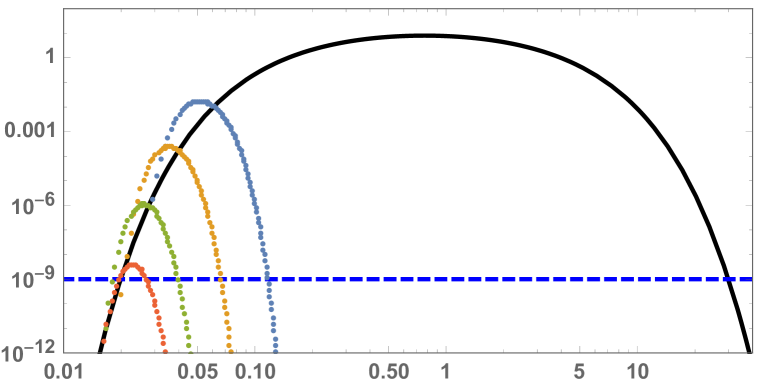
Figure 1: The sphaleron suppression rates as a function of the sphaleron size $\rho$ in ${\rm GeV}^{-1}$. The solid curve corresponds to the unbroken phase $v=0$ at $T=T_{EW}$. Four sets of points, top to bottom, are for well broken phase, at $T=155,150,140,130\,{\rm GeV}$. They are calculated via Ansatz B described in Appendix C, and normalized to lattice-based rates. The horizontal dashed line indicates the Hubble expansion rate relative to these rates.

In Fig. 1 we show the sphaleron size distribution at the critical temperature (the solid line) and four temperatures below it, in the broken phase. We see that the appearance of a nonzero Higgs VEV leads not only to a suppression of the rate, but also to a dramatic decrease of the sphaleron sizes. The lowest temperature shown, $T_{L}\approx 130\,{\rm GeV}$, corresponds to the sphaleron rate that reaches the Universe expansion rate (Hubble).

The intercept of each curve with the dashed horizontal line gives (the smallest and) the largest size sphalerons which have rates comparable to the Universe expansion rate, and should therefore be “at freezeout”, out of thermal equilibrium. One can see that for four sets of points shown, $\rho_{\rm max}$ changes from about $1/10\,{\rm GeV}$ to $1/30\,{\rm GeV}$. Very close to the critical temperature $T_{EW}$ the sphalerons may be significantly larger in size, as seen from a comparison to the black curve. However the related uncertainty does not matter, as we will show below, because in this region the CP asymmetry is extremely small, growing toward $T=130\,{\rm GeV}$.

III Sphaleron explosions: production of sound and gravity waves

Most of the studies on the gravity wave generation by the EWPT focus on scenarios based on the first order transition or the “cold” transition , as those usually yield large density fluctuations. To our knowledge, the smooth cross over transition of the minimal SM has not been considered.

Since the sphaleron explosions give rise to significant deviations from a homogeneous stress tensor of the plasma

$$\Delta T^{\mu\nu}\sim G^{\mu\lambda}G_{\lambda}^{\nu}\sim{1\over g^{4}T^{4}}$$ (18)

one may expect radiation of the gravity waves. The stress tensor from the analytically known sphaleron field (B) yields long expressions which are not suitable for reproduction here. Instead, we show in Fig. 2 the behavior of $T^{00}(t,r)$ (the energy density) and $T^{33}(t,r)$ (the pressure), which illustrates the time-development of the exploding sphaleron in a spherical shell.

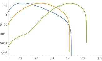
Figure 2: Components of the stress tensor (times $r^{2}$, namely $r^{2}T^{00}(t,r)$ upper plot, $r^{2}T^{33}(t,r)$ lower plot) as a function of $r$, the distance from the center, at times $t/\rho=0.1,1,2$, left to right.

The key point here is to assess the scale dependence of both the sound and gravity waves triggered by the explosion, which can be expressed using the power-per-volume $dE/d^{4}x$. Dimensional reasoning shows that the average scale is shifted to smaller sphaleron sizes. The measure for small size sphalerons

$${d\rho\over\rho^{5}}P(\rho)=d\rho\,{\rm exp}\bigg{(}-{3\pi^{2}\over g^{2}T\rho}-5{\rm log}(\rho)\bigg{)}$$ (19)

is peaked at

$$\rho_{*}={3\pi\over 20\alpha_{EW}T}\approx{1\over 10\,{\rm GeV}}$$ (20)

which is about an order of magnitude smaller than the peak of the distribution (Fig.1).

Also, for $T>T_{c}$ we do not expect direct gravitation emission from the sphaleron explosion. In this regime the Higgs VEV vanishes, nothingh breaks the rotational symmetry of the gauge field leading to spherically symmetric sphaleron explosions. As a result, these explosions cannot directly generate gravitational waves no matter how violent they are. This is not the case for $T<T_{c}$ as we discuss below.

There is an indirect way to gravitational signal as discussed in Kalaydzhyan:2014wca . Spherical sphaleron explosions do excite the underlying medium through hydrodynamical sound waves and vortices. Of course, the medium viscosity will eventually kill them, but since the damping rate scales as $\Gamma\sim\eta k^{2}$, at small $k$ (large wavelength) this time can be long. Random set of sound sources creates acoustic turbulence. Under certain conditions it may turn into the regime of inverse cascade and propagate many orders of magnitude, perhaps to the infrared cutoff, the horizon size of the Universe. It is a $2\rightarrow 1$ generic process Kalaydzhyan:2014wca

$${\rm sound+sound\rightarrow gravity\,wave}$$

which operates during the whole lifetime of the sound.

Just after the transition, at $T<T_{EW}$, a nonzero Higgs VEV leads to different masses of various quarks, leptons and gauge bosons. This “mass separator” split expanding spherical shell of the explosion into separate regions. Also, a nonzero Weinberg angle (or the nonzero $g^{\prime}$ coupling of the Higgs to the Abelian $U(1)$ field) produces an elliptic deformation of the sphaleron explosion. It is created by the following part of the action

$$\Delta S_{a}={m_{Z}^{2}-m_{W}^{2}\over 2}\int d^{4}x\sqrt{g}g_{\mu\nu}Z^{\mu}Z^{\nu}$$ (21)

where the metric is explicitly shown. Writing it as a flat metric plus perturbation $g_{\mu\nu}=\eta_{\mu\nu}+h_{\mu\nu}$ and expanding in $h_{\mu\nu}$ is the standard way to derive the corresponding stress tensor, which is

$$\Delta T^{\mu\nu}_{a}={m_{Z}^{2}-m_{W}^{2}\over 2}\bigg{(}-Z^{\mu}Z^{\nu}+{\eta^{\mu\nu}\over 2}Z^{2}\bigg{)}$$ (22)

Here, the pre-factor is proportional to $v^{2}(T)$, nonzero only after EWPT, at $T<T_{EW}$.

The power produced by the gravity wave is proportional to the squared matrix element $|M|^{2}$ of the Fourier resolved stress tensor by the gravity wave with momentum $\vec{k}$

$${\cal M}(h,k)=\int d^{4}x\Delta T^{\mu\nu}(x)\,h_{\mu\nu}{e^{ik\cdot x}\over r}$$ (23)

We recall that the polarization tensor for the gravity wave $h_{\mu\nu}$ is traceless, and transverse, i.e. nonzero only in the 2-d plane normal to $\vec{k}$. For example, for $\vec{k}$ in the 1-direction, the pertinent contributions in (23) are $T^{22}-T^{33}$ or $T^{23}$ for the respective polarizations.

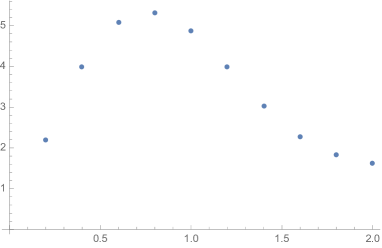
Figure 3: The dimensionless matrix element ${\cal M}/(M_{Z}^{2}-M_{W}^{2})^{2}$ in (23) versus $k\rho$, for a gravity wave propagating in the 1-direction with transverse polarization giving $T^{22}-T^{33}$.

The main part of the stress tensor gives vanishing matrix element, as it should, but the asymmetric part of the stress tensor produces gravitational radiation. In Fig.3 we show the dependence of the gravity wave matrix element as a function of $k\rho$. As expected, it is maximal at $k\rho\sim 1$. We have already evaluated the most important sphaleron size in (20). As a result, the expected gravitational wave momentum should be $k\sim 1/\rho_{*}\approx 10-30\,{\rm GeV}$.

IV CP violation and the sphaleron explosions

IV.1 Standard Model CP violation, from the phase of the CKM matrix

In this section we discuss whether the “minimal” CP violation in the SM, following from the experimentally well studied complex contribution of the CKM matrix, can generate the required level of asymmetry. Needless to say that this question was addressed by many in talks and textbooks, but it is worth reviewing it again here.

While the sphaleron decay process has been discussed at the classical level, see Appendix B, the CP-violating effects appear at one-loop level with the contribution from all generations of quarks and their interferences. We are not aware of any consistent calculation of the corresponding CP violation during the sphaleron decays.

Because of our focus on large-size sphalerons, the appropriate strategy appears to be an evaluation of the fermionic determinant in the “smooth” background of a W-field with small momenta. The determinant of the Dirac operator in such field ${\rm Log(det}(\hat{D}))$ generates the effective action, induced by one-loop fermion process, which is similar to the well known Heisenberg-Euler effective action in QED, with the CP-violating part extracted from its imaginary part.

Studies along these lines have been carried, but the results are still (to our knowledge) inconclusive. The calculation in Hernandez:2008db found no CP violation to leading order ${\cal O}(W^{4})$, but reported a nonzero contribution to order ${\cal O}(ZW^{3}DW)$ from a dimension-6 P-odd and C-even operator of the type

$$\epsilon^{\mu\nu\lambda\sigma}\left(Z_{\mu}W_{\nu\lambda}^{+}W_{\alpha}^{-}\left(W_{\sigma}^{+}W_{\alpha}^{-}+W_{\alpha}^{+}W_{\sigma}^{-}\right)+{\rm c.c.}\right)$$

(24)

containing one neutral current vertex and the $Z$-boson field. Other operators, which are C-odd and P-even, were claimed to contribute in GarciaRecio:2009zp ; Brauner:2012gu .

It is not a trivial task to find an example of the field which would give a non-vanishing expectation value for this operator. In particular, it should be T-odd, and thus involving time evolution or electric field strength. We have checked using the analytic solution for the sphaleron explosion Ostrovsky:2002cg ; Shuryak:2002qz described in Appendix B, that it does give a non-vanishing expectation value for this operator. (The formulae are unfortunately too long to be given here.)

IV.2 Scale dependence of the CP violation

The main physical issue is not so much the operator expectation values, but rather the scale dependence of the Wilsonian OPE coefficients multiplying them. These coefficients are usually rather complicated functions of the quark masses, see e.g. the explicit form of the coefficient of the operator (24) given in the Appendix of Hernandez:2008db . Instead of calculating the OPE coefficients for specific operators, we suggest a somewhat more general and universal approach, that will help us understand their scale dependence.

Consider a typical CP violating contribution to the effective action in some smooth gauge background $W_{\mu}(x),Z_{\mu}(x)$ as vertices in a one-loop fermionic contribution. Each fermion line is characterized by a Dirac operator $D/\hskip 2.58334pt$ in the gauge background. Using left-right spinor notations it has the form

$${\rm det}\left(\begin{array}[]{cc}iD/&M\\ M^{\dagger}&i\partial\!\!\!/\\ \end{array}\right)={\rm det}(i\partial\!\!\!/)\,{\rm det}\left(iD/\hskip 2.58334pt+M{1\over i\partial\!\!\!/}M^{\dagger}\right)$$ (27)

where $M$ is a mass matrix in flavor space and the slash here and below means the convolution with the Dirac matrices, e.g. $D/\hskip 2.58334pt=D_{\mu}\gamma_{\mu}$. Let us use a representation in which this operator is diagonalized

$$iD/\hskip 2.58334pt\psi_{\lambda}(x)=\lambda\psi_{\lambda}(x)$$ (28)

Its two sub-operators, $p\!\!\!/$ and $W\!\!\!\!\!/$ are not in general diagonal in this basis, but for our qualitative argument we will only include their diagonal parts

$$\left<\lambda|i\partial\!\!\!/|\lambda^{\prime}\right>\approx p\!\!\!/\,\delta_{\lambda\lambda^{\prime}},\,\,\,\,\left<\lambda|W\!\!\!\!\!/|\lambda^{\prime}\right>\approx\xi\lambda\,\delta_{\lambda\lambda^{\prime}}$$ (29)

where $p/\hskip 2.58334pt,\xi$ are in general some functions of $\lambda$. In this approximation the corresponding (Eucidean) propagator describing a quark of flavor $f$ propagating in the background can be represented as the usual sum over modes

$$S(x,y)\approx\sum_{\lambda}{\psi^{*}_{\lambda}(y)\psi_{\lambda}(x)\over\lambda+M{p\!\!\!/}^{-1}M^{+}}$$ (30)

where the right-handed operator $i\partial/\hskip 2.58334pt$ is approximated by its diagonal matrix element in the $\lambda$-basis. Throughout, we will trade the geometric mean appearing in all expressions $\sqrt{p\!\!\!/\lambda}\rightarrow\lambda$, for simplicity.

The generic fourth-order diagram in the the weak interactions, shown in Fig.4(0) contains four CKM matrices. In the coordinate representation its analytic form is form

$$\int\prod_{i}^{4}d^{4}x_{i}\,{\rm Tr}\bigg{(}W\!\!\!\!\!/(x_{1})\hat{V}\hat{S}_{u}(x_{1},x_{2})W\!\!\!\!\!/(x_{2})\hat{V}^{\dagger}\hat{S}_{d}(x_{2},x_{3})W\!\!\!\!\!/(x_{3})\hat{V}\hat{S}_{u}(x_{3},x_{4})W\!\!\!\!\!/(x_{4})\hat{V}^{\dagger}\hat{S}_{d}(x_{4},x_{1})\bigg{)}$$

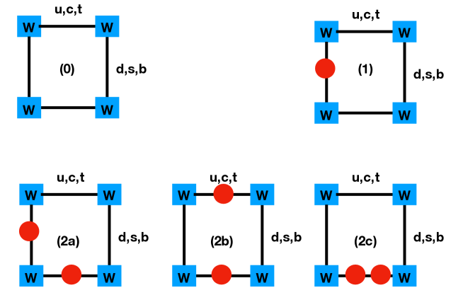
Figure 4: Schematic description of a fourth order one-quark-loop diagrams with 4-$W$ boson insertions shown in blue squares. The additional $Z_{\mu},A_{\mu}$ fields (diagram $(0)$), one $(1)$ and two ($2a,2b,2c$) are shown in red-circles.

Here hats indicate that the CKM matrix $V$ and the propagators are $3\times 3$ matrices in flavor space. The propagator also have labels $u,d$, indicating up or down type quarks. The trace is over Dirac and color indices as well: slash with $W$ field as usual mean convolution of vector potential with gamma matrices. For other diagrams of Fig.4 including $Z$ and electromagnetic $A^{em}$ fields the analytic expressions are generalized straightforwardly.

The spin-Lorentz structure of the resulting effective action is very complicated. However, to understand the pattern of interference between quarks of different flavors, producing the $CP$ violation and eventually its scale dependence, one may focus on flavor indices alone. This is possible if instead of standard $momentum$ representation of Feynman diagrams we will use the eigenbasis of the Dirac operator in the background field. Specifically, using the orthogonality condition of the different $\lambda$-modes and perform the integration over coordinates, to obtain a simple expression, with a single sum over eigenvalues $\sum_{\lambda}F(\lambda)$ with the same 4-th order box diagram in the “$\lambda$-representation” reduced to

$$F(\lambda)=\lambda^{4}{\rm Tr}\left(\hat{V}S_{d}\hat{V}^{\dagger}S_{u}\hat{V}S_{d}\hat{V}^{\dagger}S_{u}\right)$$ (31)

Note that different backgrounds have different spectra of the Dirac eigenvalues $\lambda$, and $F(\lambda)$ obtained should therefore be convoluted with appropriate background-dependent spectral densities $d(\lambda)$.

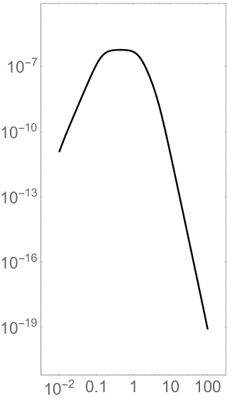
Figure 5: CP-violating contribution ${\rm Im}F_{ZZ}(\lambda)$ from the diagram $Z^{2}W^{3}DW$ versus $\lambda$ (GeV).

However, in the eigenbasis representation one can perform the multiplication of the flavor matrices and extract a $universal$ function of $\lambda$, that describes explicitly the dependence of the CP violation contribution on a given scale. Using the standard form of the CKM matrix $\hat{V}$, in terms of the known three angles and the CP-violating phase $\delta$, and also the six known quark masses, one can perform the multiplication of these 8 flavor matrices and identify the lowest order CP-violating term in the result.

After carrying the matrix multiplications in the 4-th order diagram Fig.4(0), we arrive at a complicated expression, which when expanded to the first power in the CP-violating phase does not have the $O(\delta)$ contribution. This means that the resulting effective Lagrangian does $not$ produce CP violation. This conclusion is not new, as it was (to our knowledge) first obtained a decade ago in Hernandez:2008db .

Since we do $not$ expect this cancellation between various quark flavors to hold for all 4-W insertions plus arbitrary neutral $Z$ and electromagnetic $A^{em}$ fields, we consider the lowest order insertions to the one-quark-loop as shown Fig.4 by red circles. The insertion of a Z-vertex is flavor independent and only double $\hat{S}\rightarrow\hat{S}\hat{S}$ or triple $\hat{S}\rightarrow\hat{S}\hat{S}\hat{S}$ the quark propagators as in diagram (2c). The electromagnetic field insertions carry quark electric charges, $e_{u}=2/3$ and $e_{d}=-1/3$.

The explicit flavor traces for these higher order diagrams show that (1,2b,2c) do not lead to CP-violating $O(\delta)$ terms in the resulting effective Lagrangian also. The only one that does is diagram (2a), with the result

$${\rm Im}F(\lambda)=\lambda^{6}{\rm Im\,Tr}\left(\hat{V}S_{d}\hat{V}^{\dagger}S_{u}\hat{V}S_{d}ZS_{d}\hat{V}^{\dagger}S_{u}ZS_{u}\right)$$

$$=2\lambda^{6}{J(m_{b}^{2}-m_{d}^{2})(m_{b}^{2}-m_{s}^{2})(m_{d}^{2}-m_{s}^{2})(m_{c}^{2}-m_{t}^{2})(m_{c}^{2}-m_{u}^{2})(m_{t}^{2}-m_{u}^{2})\over\Pi_{f=1..6}(\lambda^{2}+m_{f}^{2})^{2}}$$ (32)

We recall that $J$ is the famed Jarlskog combination of the CKM cos and sin of all angles times the sin of the CP violating phase.

Note that the $x$-dependent gauge fields $W_{\mu},Z_{\mu},A^{em}_{\mu}$ in the vertices should be convoluted with the currents in the eigenstates $\bar{\psi}_{\lambda}(x)\gamma_{\mu}\psi_{\lambda}(x)$. Diagram (2a) with 2-$Z$ and 2-$A^{em}$ would then carry the extra factor

$$C_{2a}=\big{(}(Z_{\lambda})^{2}-{2\over 9}(A^{em}_{\lambda}))^{2}\big{)}$$ (33)

Since these two terms have opposite signs, no universal statement about the $sign$ of the CP violation in arbitrary background can be made.

In Fig.5 we show (IV.2) as a function of the eigenvalue scale $\lambda$. It is clear that the magnitude of the CP violation depends on the absolute scale very strongly. When the momentum scale is at the electroweak value $\sim 100\,{\rm GeV}$ (the r.h.s. of the plot), it is $10^{-19}$. But in the “sweet spot”, between the masses of the light and heavy quark $\lambda\in(0.2-2)\,{\rm GeV}$, the asymmetry is suppressed only by about $\sim 10^{-6}$.

V Higher order plasma effects

In the preceding section we discussed a generic effective Lagrangian in arbitrary background fields. In fact we only need to focus on one particular background, that originating from a sphaleron explosion, so we start by identifying its specific properties.

It is a $classical$ field, with $W_{\mu},Z_{\mu},A^{em}_{\mu}\sim O(1/g_{EW})$, and therefore the only smallness in the effective Lagrangian extracted from the one-quark-loop is $\sim O(g_{EW}^{0})$, while the sphaleron action is $\sim O(1/g_{EW}^{2})$. The perturbative treatment of $W$ is related to the fact that we are looking for a very small CP violation resulting from the CKM matrix. The perturbative treatment of $Z_{\mu},A^{em}_{\mu}$ is not a priori justified. It only helps in locating the lowest order nonzero diagrams.

The sphalerons and their explosion have so far been considered classically, via appropriate solutions of the Yang-Mills (and Dirac) equations. The most symmetric case Shuryak:2002qz (see Appendix) corresponds to symmetric phase $T>T_{EW}$ in which there is no Higgs VEV and the gauge fields are only the $SU(2)$ ones, without electromagnetic ones.

Yet the actual sphaleron explosions happen in a primordial plasma. The generic argument is that the gauge fields are classical $W,Z\sim O(1/g_{EW})$ while thermal fields of the plasma are $\sim O(g_{EW}^{0})$ , so in the leading order they are not modified. However, since we consider sphalerons of different sizes, there appears a parameter $\rho T$. On top of it, thermal fields have large number of degrees of freedom, so the corrections to a classical approximation needs to be studied.

The issue gets more urgent at the level of the one-loop quark-induced action we need to study for CP violation. Quark fields, unlike gauge ones, are not classical. The eigenmodes we consider are all normalized to a unit value. Plasma-induced polarization (mass) operators come not only from weak interactions, but from thermal gluons as well. Therefore the formal suppression parameter is $\sim\alpha_{s}$, which not so small. A full inclusion of all Dirac modes following a sphaleron explosion in a plasma is still beyond the scope of this work. In this section we provide a qualitative discussion and estimates.

V.1 Electric screening

Let us recall the argument put forth at the beginning of section II.3.1: since the sphalerons are magnetic objects, they can be as large as allowed by the magnetic screening mass,

$$\rho\leq{1\over M_{m}}\sim{1\over g^{2}T}$$

Thus, it can differ from the basic thermal scale $T$ by about two orders of magnitude. However, a sphaleron explosion generates an (electroweak) electric field as well. Originally directed radially, that accelerates quarks and leptons from their initial state as zero modes, to their positive and physical energy final states, violating baryon and lepton number. In the final stage, only the transverse electric fields remain, producing physical $W,Z$ that are transversely polarized to the radial direction. We recall that under these conditions all particles are massless or have small masses, as the Higgs VEV is zero or small.

The electric screening mass is $M_{E}\sim gT$, so the screening length is about $g$ times shorter than the magnetic screening length. The “plasma on-shell masses” of $W,Z$ are also $M_{W,Z}\sim gT$. Both effects are incorporated by an additional thermal contribution to the effective Lagrangian (in momentum representation)

$$\Delta L_{plasma}={1\over 2}\Pi_{\mu\nu}(T,k_{\sigma})A^{\mu}(k_{\sigma})A^{\nu}(k_{\sigma})$$ (34)

with the one-loop polarization operator $\Pi$ calculated already in Ref.Shuryak:1977ut . So, what qualitative modification these electric thermal effects produce?

Classically, the sphaleron explosion produces $W,Z$ with momenta $p\sim 1/\rho$, and their total number is of the order of the action $N_{W<Z}\sim 1/g^{2}\sim 100$. In the thermal plasma this is no longer possible. The available energy is not sufficient to produce that many gauge quanta since their thermal masses are $M_{W,Z}\sim gT$. Furthermore, at the momenta $p\sim 1/\rho$ corresponding to the initial sphaleron sizes, the plasma modes are not $W,Z$ plasmons but rather collective modes of hydrodynamical origin, corresponding to the longitudinal sounds (phonons) and transverse (rotational and purely diffusive) motions. (How exactly the energy is divided between those modes we have not assessed yet: it may be needed for gravity wave predictions).

As we already noted earlier, due to the nonzero Weinberg angle, some part of sphaleron energy goes to QED electromagnetic fields and eventually to polarized magnetic clouds. Their polarization tensor includes not the electroweak but the electric coupling constant, which is smaller, and so their interaction with the plasma can probably be neglected, once they are produced.

V.2 How do plasma effects modify quark/lepton production and respective $B,L$ number violations ?

In the primordial plasma, fermions are also modified by their interactions with the thermal medium. While leptons have electroweak interactions only, quarks interact strongly with ambient gluons, with much a stronger coupling constant $g_{s}$. Therefore quark modes acquire larger masses, and one may wander if those can prevent the $B,L$ number violation phenomenon itself.

At this point, a historical comment may be made. When Farrar and Shaposhnikov Farrar:1993hn realized that the CP violation induced by the CKM matrix have the “sweet spot” mentioned above, they focused on the dynamics of the quarks with small momenta $p\sim 1\,{\rm GeV}\ll T$. Specifically, they argued that under certain conditions the strange quarks are totally reflected from the boundary of the bubble (they assumed the transition to be first order), while the up/down quarks are not. This scenario has been later criticized, based on higher order corrections to the quark dispersion curves, and the conclusions in Farrar:1993hn , have been refuted. For pedagogical reasons, let us split the refuting arguments in three, reflecting on their increase sophistication.

The first argument says that the Euclidean thermal formulation with anti-periodic fermionic boundary conditions, implies that the minimal fermionic energies are set by the lowest Matsubara mode

$$\omega_{M}=\pi T\sim 300\,{\rm GeV}$$ (35)

Indeed the typical fermionic momenta are of this order, and the CKM-induced CP violation at this scale is $\sim 10^{-19}$ as we detailed above.

The second argument is based on the emergence of a “thermal Klimov-Weldon” quark mass

$$M_{KW}={g_{s}T\over\sqrt{6}}\sim 50\,{\rm GeV}$$ (36)

induced by the real part of the forward scattering amplitude of a gluon on a quark.

Both arguments were essentially rejected by Farrar and Shaposhnikov, who pointed to the fact that while both effects are indeed there, there are still quarks with small momenta $p\ll T,M_{q}$ in the Dirac spectrum.

The third argument which is stronger, was given in Gavela:1993ts ; Huet:1994jb . It is based on the decoherence suffered by a quark while traveling in a thermal plasma, as caused by the imaginary part of the forward scattering amplitude (related by unitarity to the cross section of non-forward scatterings on gluons). Basically, they argued that if a quark starts with a small momentum, it will not be able to keep it small for necessary long time, due to such scattering. The imaginary part is about

$${\rm Im}(M_{q})\sim\alpha_{s}T\sim 20\,{\rm GeV}$$ (37)

We now return to the sphaleron explosions we have presented, and ask how such plasma effects can affect their quark production. The most obvious question is that of “insufficient energy”. Indeed, if each quark carries a “thermal Klimov-Weldon mass” as the smallest energy at small momenta, is there even enough energy to produce the expected 9 quarks? Alltogether, these 9 masses amount to about $450$ GeV, which is comparable to the total sphaleron mass (11) at a size $\rho\sim 1$ GeV^-1. Therefore, the classical treatment used above, in which the back-reaction of the quarks on the explosion were neglected, by solving the Dirac equation in a background field approximation, should be significantly modified.

However, there is a simple way around the “insufficient energy” argument. In thermal field theory the sign of the imaginary part of the effective quark mass operator can be both positive or negative. This corresponds to the fact that instead of producing new quarks, the sphaleron amplitude can instead absorb thermal antiquarks from the plasma.

Still we would argue that, unlike the Farrar-Shaposhnikov scenario Farrar:1993hn , our sphaleron-induced baryon number violation should survive all plasma effects. We do not classify quarks by their momenta, but rather by the virtualities or eigenvalues of the Dirac operator $\lambda$, in the background of sphaleron explosion solution.

It is true that the plasma effect will modify the spectral density $P(\lambda)$ in a way, that most of the virtualities $\lambda$ are equal or larger than the thermal Klimov-Weldon mass (36 )

$$|\lambda|>M_{KW}$$

According to Fig. 5, this puts the CP asymmetry to be of order $\sim 10^{-17}$, way too small for BAU.

However, a sphaleron explosion is a phenomenon in which gauge topology of the background field is changing. The topological theorems requires the existence of a zero mode of the Dirac operator in the spectral density, $P(\lambda)\sim\delta(\lambda)$. (Another way to say it, is to recall that the sphaleron explosion implies changing of the Chern-Simons number, which is locked to the change in the quarks and leptons left-polarization by the chiral anomaly.) Plasma effects do indeed modify the gauge fields during the sphaleron explosion, perhaps strongly, $O(1)$ in magnitude, but they cannot change their topology. Therefore plasma effects cannot negate the existence of the zero mode: it is robust, completely immune to perturbations.

For a skeptical reader, let us provide an example from practical lattice gauge theory simulations, which may perhaps be convincing. At temperature at and above the critical $T>T_{c}$, in a QGP phase, there are plenty of thermal gluons. And yet, when a configuration with the topological charge $Q=\pm 1$ is identified on the lattice, an exact Dirac eigenvalue with $\lambda=0$ is observed, within the numerical accuracy, typically $10^{-9}$ or better. Also, the spatial shape of this eigenvalue is in very good agreement with that calculated using semiclassical instanton-dyons Larsen:2018crg . Zillions of thermal gluons apparently have no visible effect on the shape of these modes, in spite of the fact that the gauge fields themselves are undoubtedly strongly modified. Of course, this example is in an Euclidean time setting, while the sphaleron explosion is in a Minkowskian time setting. Real time simulations are much more costly and have only been done with gauge fields without fermions. However, we are confident that baryon number violation itself is completely robust, immune to thermal modifications.

V.3 Dirac zero mode and related CP violation

Now that we argued that the Dirac operator should still have an exact zero mode for a sphaleron explosion, even in the plasma, we now further ask how its presence in the Dirac operator determinant can affect the estimates of the CP violation we made earlier.

V.3.1 Dirac zero mode

Let us return to the Dirac operator (27 ), in left-right notations. The quark-gluon scattering is vectorial, so the Klimov-Weldon mass (or more generally, the forward scattering amplitude at an appropriate momentum) should be added to the (LL) and (RR) diagonal elements

$${\rm det}\left(iD/\hskip 2.58334pt+M_{KW}+M_{LR}{1\over i\partial\!\!\!/+M_{KW}}M^{\dagger}_{RL}\right)\\$$

Note that the non-diagonal fermion masses (LR and RL) flipping chirality can only come from interaction with the Higgs scalar field, violating chiral symmetry. When there is no Higgs VEV (at $T>T_{c}$), to lowest order the last term is absent. At next order, it is proportional to the corresponding Yukawa couplings for different fermion species.

What we argued above, means that the plasma-deformed first LL operator $iD/\hskip 2.58334pt+M_{KW}$ should, like the vacuum version, have a zero eigenvalue. For that, we write

$$iD/\hskip 2.58334pt=(i\partial\!\!\!/+gA_{\mu})\hat{1}+gA_{\mu}(\hat{M}_{CKM}-\hat{1})$$ (38)

where hats indicate matrices in quark flavors. The topological zero mode $\lambda=0$ follows from the flavor-diagonal part, as a zero eigenvalue of the first bracket

$$(i\partial\!\!\!/+gA_{\mu}\hat{1})\psi_{\lambda}=\lambda\psi_{\lambda}$$ (39)

The so called “topological stability” implies that the zero eigenvalue does not have any perturbative corrections.

The remaining part of the Dirac operator (38) can formally be considered small and thus treated perturbatively, providing small modification of the known explicit solution to the Dirac equation in the background of sphaleron explosion. The deviation of the gauge field term from $\hat{1}$ through

$$gA_{\mu}(\hat{V}_{CKM}-\hat{1})$$

would provide vertices for flavor changing quarks, and the mass term, in the form

$$M_{LR}{1\over i\partial\!\!\!/+M_{KW}}M^{\dagger}_{RL}$$

would provide perturbative corrections to the quark propagators connecting these vertices. As we will see, this flavor-dependent part is key for evaluating the magnitude of CP violation.

V.3.2 Quark production probability

As explained by ’t Hooft long ago tHooft:1976snw , the physical meaning of the zero mode of the instanton (or its analytic continuation to Minkowski time Shuryak:2002qz we imply here) is the wave function of the outgoing fermion produced. The CP violation induced by the quarks “on their way out” appear due to interferences of certain diagrams with different intermediate states. In short, the production probabilities of quarks and antiquarks are not equal. The method to calculate the effect was previously developed by Burnier and one of us Burnier:2011wx .

Consider an outgoing quark, accelerated by the electric field of the sphaleron explosion, and interacting on its way with the $W$ field twice. The full probability for the quark production contains sums over all possible intermediate flavor states. For example, if the quark started as $b$-quark, then one has a triple sum over intermediate flavors

$$P_{b}=\sum_{IJK}\bigg{(}A\bigg{(}b\rightarrow I=t,c,u\rightarrow J=b,s,d\bigg{)}\times A\bigg{(}J=b,s,d\leftarrow K=t,c,u\leftarrow b\bigg{)}\bigg{)}$$ (40)

We now note the three key features of this expression:

(i) the intermediate up-quarks $t,c,u$ in each amplitude need not be the same. The interference of multiple paths in flavor space, induced by the CKM matrix angles, may lead to CP violation;
(ii) the total number of CKM matrices $\hat{V}_{CKM}$ is four, which is just enough to make this CP violating contribution nonzero;
(ii) the combination $\hat{V}_{CKM}^{+}\hat{V}_{CKM}\hat{V}_{CKM}^{+}\hat{V}_{CKM}$ and its complex conjugate is not the same as for the corresponding ($\bar{b}$) antiquark.

In light of this, the probability to produce a quark and an antiquark are not equal, i.e. $AA_{q}\neq\overline{AA_{q}}$. More specifically, let us write the convolution for a particular initial up-quark state labeled as $U0$,

$$AA_{U0}\sim \sum_{D1,U,D2}{\rm Tr}\bigg{(}\hat{P}_{U0}W(x_{1})\hat{V}_{CKM}S^{D1,D1}(x_{1},x_{2})$$

$$\times W(x_{2})\hat{V}_{CKM}^{+}\tilde{S}^{U1,U1}(x_{2},x_{3})W(x_{3})\hat{V}_{CKM}S^{D2,D2}(x_{3},x_{4})W(x_{4})\hat{V}_{CKM}^{+}\hat{P}_{U0}\bigg{)}$$ (41)

where $\hat{V}_{CKM}$ is a $3\times 3$ CKM matrix (indices not shown) and $P_{U0}$ at both ends are projectors onto the original quark type. The propagators $S(x,y)$ are diagonal flavor matrices with their indices shown. There are 3 options for each index, $D1,D2=b,s,d,$ and $U0,U1=t,c,u$, so for each quark the probability has $3^{3}=27$ interfering terms. The intermediate propagator $\tilde{S}^{U1,U1}$ has tilde, which indicates that it should include the propagation from point $x_{3}$ to infinity, and its conjugate propagation from infinity to point $x_{4}$. Therefore, its additional phase depends on the distance between these points. The corresponding amplitudes for the antiquarks involve complex conjugate (not Hermitian conjugate!) CKM matrices relative to the quark amplitude, namely

$$\overline{AA}_{U0}\sim \sum_{D1,U,D2}Tr\hat{P}_{U0}W(x_{1})\hat{V}_{CKM}^{*}S^{D1,D1}(x_{1},x_{2})$$ (42)

$$\times W(x_{2})\hat{V}_{CKM}^{T}\tilde{S}^{U1,U1}(x_{2},x_{3})W(x_{3})\hat{V}_{CKM}^{*}S^{D2,D2}(x_{3},x_{4})W(x_{4})\hat{V}_{CKM}^{T}\hat{P}_{U0}$$

The difference in the probability of production of a quark and antiquark is denoted by

$$\Delta P_{Q}\equiv{\rm Im}\big{(}AA_{Q}-\overline{AA}_{Q}\big{)}$$

We now note that:

(i) the propagators of quarks of different flavors between the same relative points have different phases;
(ii) the locations in the amplitude $x_{1,2}$ need not be the same as the locations $x_{3,4}$ in the conjugate amplitude, so in principle we need to integrate over all of these locations independently.

For a qualitative estimate of (V.3.2-42) we write the nontrivial flavor-dependent phases in the propagators as

$$S^{QQ}=e^{i\phi_{Q}}$$

suppressing for an estimate their dependence on the coordinates, and perform the sums with $U0$ referring to all 6 initial types of quarks. The lengthty result is given in Appendix C. As already indicated, these phases come from the last term in the Dirac operator. Apart of common phase induced by the $p/\hskip 2.58334pt$ in it, there are flavor-dependent phases induced by the last term in the Dirac operator

$$\phi_{Q}={m_{Q}^{2}|x_{1}-x_{2}|\over M_{KW}}$$ (43)

Using for coordinate distance travelled the sphaleron size (maximal at freezout line)

$$|x_{1}-x_{2}|\approx\rho_{max}\sim 1/10-1/30\,{\rm GeV}^{-1}$$

we introduce a new (temperature-dependent) mass scale

$$M_{\rho}\equiv\left({M_{KW}\over\rho_{max}(T)}\right)^{1/2}\sim 40\,{\rm GeV}$$ (44)

Using this notation, the additional phases is just a ratio of (flavor and temperature-dependent) quark mass to $M_{\rho}$, squared:

$$\phi_{Q}={m_{Q}^{2}\over M_{\rho}^{2}}$$ (45)

When the quark masses are smaller than $M_{\rho}$, the corresponding phases are small.

V.3.3 Amount of CP violation

Let us now recall that we are discussing the Universe at temperatures across the electroweak transition, with the Higgs VEV $v(T)$ emerging from zero to eventually its value in the broken phase as we have it today. For a specific expression see the lattice result (73). All quark masses grow in proportions to the VEV, and therefore the ensuing CP violation grows. We will divide this stage of the evolution into two stages.

Stage 1: In the quark production probabilities, the four vertices with CKM matrices are connected by three propagators, leading to expressions cubic in $\phi_{Q}\sim(m_{Q}/M_{\rho})^{2}$, after expanding the expressions in Appendix C. The end of stage 1 happens when the largest of the phases, that due to the top quark, reaches $O(1)$, or

$$m_{t}\approx M_{\rho}\sim 40\,{\rm GeV}$$ (46)

At this time all other quark masses are much smaller than the top quark mass, respective to their Yukawa couplings, and their phases are therefore small. The lengthy expressions in Appendix C can be simplified by expanding these exponents to first order in the phases. Say, the one for $d$ quark contains the heaviest quark masses in the expression, and the corresponding CP asymmetry is

$$\sim 2J{m_{b}^{2}(T)m_{c}^{2}(T)\over M_{\rho}^{4}(T)}\sim 2J\bigg{(}{m_{b}^{2}(0)m_{c}^{2}(0)\over m_{t}(0)^{4}}\bigg{)}\bigg{(}{m_{t}(0)^{4}\over M_{\rho}^{4}}\bigg{)}\approx J\cdot 1.2\cdot 10^{-7}\cdot 350\sim 10^{-9}$$ (47)

Stage 2: This corresponds to a large top quark mass $m_{t}>M_{\rho}$ and the phase $\phi_{t}\gg 1$, with a rapidly oscillating exponent. Therefore, we assume

$$e^{\pm i\phi_{t}}\approx 0$$

and drop all factors with top quark phase. If one starts from a light quark $U0=u$, the resulting expression contains the mass differences with the heaviest remaining masses of $b,c$ quarks, namely

$$2J{(m_{b}^{2}-m_{s}^{2})(m_{c}^{2}-m_{u}^{2})\over M_{\rho}^{4}}$$ (48)

It is similar to the expression we had before, but with masses continuing to grow. The numerator grows as the fourth power of VEV $\sim v(T)^{4}$, and the denominator approximately as its second power due to sphaleron size shrinkage. As a result, the temperature dependence is $\sim v^{2}(T)\sim(T_{EW}-T)$.

Eventually, the temperature falls to $T=130\,GeV$ below which the sphalerons freezeout completely. The prefactor $2J\sim 6\cdot 10^{-5}$ and the CP asymmetry (48) is about

$$A_{CP}\sim 0.25\cdot 10^{-9}$$ (49)

comparable to what one gets by the end of stage one.

Some remarks are now in order here. Note that if one starts with the first generation $u$ quark, the intermediate ones kept are $b$ and $c$, of the third and second generations. So, as required, all three generations are involved. Yet this does not mean that all 6 quark flavors need to be involved: in particular the answer $\Delta P_{u}$ (in Appendix D) contains a factor $(m_{b}^{2}-m_{s}^{2})$ but not $(m_{d}^{2}-m_{s}^{2})$, as there is no $d$ quark anywhere. Thus there is no $m_{s}^{2}$ in our answer. The situation is exactly the same as in the exclusive $b$ decays as we discussed earlier. Only the masses of the quarks explicitly involved in the process, not all 6 mass differences, needs to be present. The full Jarlskog mass factor is not required in exclusive reactions.

Yet the symmetry between quarks strikes back: the CP violation for the $d$ quark, $\Delta P_{d}$ (in Appendix D), has the same magnitude of the CP violation (48) but have the opposite sign. Therefore, in the symmetric phase at $T>T_{EW}$, when orientation of the sphaleron zero mode in $SU(2)$ group space is spherically symmetric, one has cancellation of the CP violations, between contributions of sphalerons which produce more $u$ or more $d$ quarks. Such cancellations is similar to what is seen in leading order effective Lagrangians, and they are is expected to be violated if higher order effects, e.g. including electromagnetic interactions, are taken into account.

As the $SU(2)$ symmetry gets broken at $T<T_{EW}$ (the phase we discuss), there is no more any symmetry between up and down weak isospin orientations. Specific Lagrangian for quark interaction with $Z$ field takes the well known form

$$L_{\bar{q}qZ}=-{g\over 2cos(\theta_{W})}\sum_{i}\bar{q}_{i}Z_{\mu}\gamma^{\mu}(g^{i}_{V}-g^{i}_{A}\gamma^{5})q_{i}$$ (50)

in which vector and axial constant are different for up and down quarks:

$$g_{V}^{i}=t(i)-2Q_{i}sin^{2}(\theta_{W}),\,\,\,g_{A}^{i}=t(i)$$

where $t(\pm)=\pm 1/2$ is weak isospin and $Q_{i}=(2/3,-1/3)$ are quark electric charges. Therefore the $u$ and $d$ CP-violating terms do $not$ cancel each other. Since $Q_{u}-Q_{d}=+1$ and sine of the Weinberg angle ${\rm sin}(\theta_{W})\approx\frac{1}{2}$ are both of order 1, the effective CP violation in the sphaleron explosion remains of order $10^{-9}$.

(The exact magnitude and, most importantly, the absolute sign of baryon number produced, require calculation of the convolution of quark zero mode with background $Z$ field of the sphaleron explosion, which is beyond the boundaries of this paper.)

Completing this section, let us recapitulate the assumptions made, and provide additional comments on further steps of this program: 1/ we used the sphaleron size $\rho$ as a placeholder for the distance between points at which the fields appear. In real calculation, coordinates should be integrated over with projections to currents, in an actual Feynman diagram defined on top of the fermionic zero mode of sphaleron explosion; 2/ we eliminated the term with the largest phase, that with the top quark mass, assuming that the oscillating term leads to the cancellation of all terms and zero answer. This contribution can be studied further;

Note that we are discussing the cosmological time near the phase transition, the quark masses under consideration are not fixed but vary in time, from zero to their physical values in the broken phase, due to a changing Higgs VEV $v$. Suppose we consider the situation in which the largest phase is of order one. We estimate this to happen when

$$m_{t}(T)\sim\sqrt{E/\rho}\sim M_{\rho}$$ (51)

This delicate estimate is straightforward in logic, but relies on a key assumption, namely that the energy of the outgoing quark is larger than $E\sim M_{KW}$. Naively, it cannot be smaller for free quarks in the electroweak plasma, as their interaction with the gluons makes their energy of order $M_{KW}$ even at zero momentum. Yet this assumption can be amended by the fact that the outgoing quarks are not free. They are still in the sphaleron field where it is worth recalling that they satisfy

$$\big{(}-D^{2}+g^{2}G_{\mu\nu}\sigma^{\mu\nu}\big{)}\psi_{\lambda}=\lambda^{2}\psi_{\lambda}$$ (52)

which contains not only the momentum squared, but also the $g^{2}A^{2},g^{2}G_{\mu\nu}$ term. For a sphaleron, the latter is about $\sim 10/\rho^{2}$, with the sign depending on the location. Therefore, the eigenvalue spectrum does not start at $\lambda>M_{KW}$ sharply, but extends to smaller values. Indeed, the quarks produced are pulled from the lower continuum, or the Dirac sea.The numerical value estimated above contains $1/\lambda^{4}$, and thus the result depends on the tail of the spectral density at smaller $\lambda$.

VI Baryogenesis

VI.1 Which sphaleron transitions are out of equilibrium?

Before we discuss freezeout of the sphaleron transitions, it is instructive to recall an analogous case of freezeout of the “little Bang” in heavy ion collisions. A good example is the production of antinucleons $\bar{N}$. In the 1990’s the cascade codes predicted small yield of $\bar{N}$, based on the fact that on average many baryons surround an anti-nucleon. Since the annihilation cross section $\sigma_{N\bar{N}}$ is large, the anti-nucleon lifetime $\tau\sim 1/(n_{N}\sigma_{N\bar{N}}\langle v\rangle)$ must be quite short. However, the data showed otherwise, with a number of produced anti-nucleons much larger than predicted by the numerical codes. The explanation was given in Rapp:2000gy . The annihilation creates multi-pion final states with $N_{\pi}\sim 6$, and the inverse reaction $N_{\pi}\rightarrow N\bar{N}$ was ignored because of certain prejudice, that the multi-particle collision has negligible rate. Explicit calculations showed otherwise, in agreement with detailed balance in thermal equilibrium.

This equilibrium is only violated after the so called chemical freezeout, when the rate $\Gamma_{inelastic}$ of the inelastic reactions changing $N_{\pi}$ and $N_{N}$ gets smaller than the expansion rate of the fireball $H=\partial_{\mu}u^{\mu}$ (the Hubble of the Little Bang). While the particle numbers become time independent, the thermal state of the expanding fireball is described via time-dependent chemical potentials, $\mu_{\pi}(t)$ and $\mu_{N}(t)$. The annihilation channel contains the fugacity factor ${\rm exp}(-2\mu_{N}/T)$, while the inverse reaction channel contains the fugacity ${\rm exp}(-N_{\pi}\mu_{\pi}/T)$. Since

$$N_{\pi}\mu_{\pi}>2\mu_{N}$$ (53)

the inverse production process gets more suppressed than the direct annihilation process. Only then, the anti-baryon population starts to be somewhat depleted.

We now return to Sakharov^′ s conditions for BAU, the deviation from thermal equilibrium. The sphaleron transitions basically consist of two different stages. The first is a complicated diffusion of the gauge fields moving uphill (say from $N_{CS}=0$ to $\frac{1}{2}$) by thermal fluctuations, driving the fields to the sphaleron configuration at $N_{CS}=1/2$. Fortunately, we do not need to understand it. In equilibrium the sphaleron population is given by the Boltzmann factor ${\rm exp}({-E_{\rm sp}/T})$. The second is the sphaleron decay rolling downhill , say from $N_{CS}=\frac{1}{2}$ to 1, as described by the real-time solution of the equations of motion in Appendix C. The process is purely Minkowskian with an amplitude $e^{iS}$ and a real action, hence unit probability of realization.

In equilibrium, the principle of the detailed balance requires that the inverse reaction with $t\rightarrow-t$, has the same rate. It means that, contrary to prejudice it may still take place, where a large number of gauge quanta

$$N_{W}\sim 1/\alpha_{EW}\gg 1$$

plus the 12 fermions required by the anomaly relation, can collide together, putting the field back on top of the sphaleron hill. As Sakharov argued, the presence of CP and thus T-violation in the process matrix element does not matter. Thermal occupation factors depend only on masses/energies, which are CP invariant.

However, since the Universe is expanding at a Hubble rate $H\sim 1/t_{EW}$, some of these transitions involve particle changing rates smaller than the Hubble rate. They are out of equilibrium! Earlier, we have shown that as a function of the sphaleron size $\rho$, the sphaleron decays get frozen when

$${\rm exp}\bigg{(}-B_{\rm sph}\rho v^{2}(T)\bigg{)}<10^{-9}$$ (54)

We now argue that the inverse process is frozen differently, so that the the equilibrium condition and its detailed balance become violated.

More specifically, for the large-$\rho$ tail and in the small-$v$ regime near $T_{c}$, the inverse reaction of multi-quanta collisions gets frozen first. The argument is based on the observation that the corrections to the sphaleron mass $\Delta E_{\rm sp}=C_{\rm sp}\rho v^{2}$ is smaller than the modification of the thermal Boltzmann factor of the inverse reaction. The latter can be written as corrections to ultra-relativistic energies of W bosons due to their mass $E_{p}\approx p+M_{W}^{2}/2p$, so the energy in their thermal exponent changes by

$$\Delta E_{W}=\sum_{i=1}^{N_{W}}\Delta E_{i}\approx\frac{N_{W}}{2p}\bigg{(}\frac{M_{W}(0)}{v(0)/v(T)}\bigg{)}^{2}$$ (55)

after rescaling the W-mass. Since $1/p\sim\rho$, this correction is of order $\sim\rho v^{2}$, but the coefficient $N_{W}$ is parametrically larger with $N_{W}\sim 100={\cal O}(1/\alpha_{EW})$.

VI.2 Contribution to BAU from out-of-equilibrium sphalerons

Our next step is to calculate the BAU produced by the large-size sphalerons which are out of equilibrium. As detailed above, this requires moving to the freezeout point, thereby sacrificing 9 orders of magnitude in the rate with $F_{\rm freezeout}\sim 10^{-9}$. This is the regime where the sphalerons decay but are not regenerated. Each electroweak sphaleron changes the baryon number by 3 units , i.e. 9 quarks each carrying $\frac{1}{3}$ baryon charge. The baryon number density normalized to the entropy density of matter, follows by integrating the rate over the freezout time $\Delta t_{FO}$

$$\bigg{(}{n_{B}\over s}\bigg{)}=3A_{CP}\times\bigg{[}{\Gamma\,F_{\rm freezeout}\over T_{EW}s_{EW}}\bigg{]}\times\bigg{[}T_{EW}t_{EW}\bigg{]}\times\bigg{[}{t_{FO}-t_{EW}\over t_{EW}}\bigg{]}$$ (56)

Here $A_{CP}$ is the CP asymmetry, the relative difference between baryon number production and annihilation in a single sphaleron transition. The second factor in square bracket is the out-of-equilibrium sphaleron rate normalized to the total entropy density $s_{EW}/T_{EW}^{3}=\frac{2\pi^{2}}{45}\,106.75$, which amounts to about $3.2\cdot 10^{-18}$. The next factor is the cosmological time in units of the electroweak temperature, which is long and about

$$T_{EW}t_{EW}\approx 2.2\cdot 10^{15}$$ (57)

The fourth (last) bracket is the available time till freezeout normalized to the total time. Using Friedmann evolution numbers in Appendix A one gets

$${t_{FO}-t_{EW}\over t_{EW}}\approx 0.5$$ (58)

Since the entropy in the adiabatic expansion of the Universe is conserved, it is the same at the BBN time which is mostly in form of black body photons. Standard Bose gas relation between the entropy density and the photon density is $n_{\gamma}=0.1388s_{\gamma}$. Substituting all these estimates in (56) gives the baryon-to-photon ratio

$$\bigg{(}{n_{B}\over n_{\gamma}}\bigg{)}=7.6\cdot 10^{-2}A_{CP}$$ (59)

Since the phenomenological value for this ratio, from the BBN fits, is known to be

$$\bigg{(}{n_{B}\over n_{\gamma}}\bigg{)}_{BBN}=6\cdot 10^{-10}$$ (60)

we conclude that the amount of CP violation required to produce the observed BAU is

$$A_{CP}\approx 0.8\cdot 10^{-8}$$ (61)

Our estimates of the CP asymmetry above gave about $A_{CP}\sim 10^{-9}$, an order of magnitude smaller than needed to explain BAU. We think that this discrepancy is still inside the uncertainty of our (quite crude) estimates (61).

VII Helical magnetogenesis

The symmetry breaking by the Higgs VEV at $T<T_{c}$ leads to mass separation of the original non-Abelian field $A_{\mu}^{3}$ into a massive $Z_{\mu}$ and a massless $a_{\mu}$, related by a rotation involving the Weinberg angle. The expanding outer shell of the sphaleron explosion contains massless photons and near-massless quarks and leptons $u,d,e,\nu$.

The anomaly relation implies that the non-Abelian Chern-Simons number during the explosion defines the chiralities of the light fermions, which can be transferred to the so called magnetic helicity

$$\int d^{3}xAB\sim B^{2}\xi^{4}\sim{\rm const}$$ (62)

The configurations with nonzero (62) are called helical. We conclude that the primordial sphaleron explosions may seed the helical clouds of primordial magnetic fields. Since the sphaleron rate is small, $\Gamma/T^{4}<10^{-7}$, these seeds are produced independently from each other, as spherical shells expanding luminally.

VII.1 The “inverse cascade” of magnetic fields

The requirement for the inverse cascade effect is chiral unbalance which is at the origin of the CME. Locally the trapped and co-moving light fermions produced by the sphaleron explosion are chiral. The time during which chirality is conserved is given by the appropriate fermion masses. For magnetic fields it is the electron mass, which at the sphaleron freezeout time is

$${m_{e}(T_{FO})}=m_{e}{v(T_{FO})\over v(0)}\sim 20\,{\rm KeV}$$ (63)

The size growth of the chiral (linked) magnetic cloud is diffusive. For a magnetically driven plasma with a large electric conductivity $\sigma$, a typical magnetic field $\vec{B}$ diffuses as

$$\frac{d\vec{B}}{dt}=D\nabla^{2}\vec{B}$$ (64)

with the diffusion constant $D=1/(4\pi\sigma)\sim 1/T$. It follows that the magnetic field size grows as

$$R^{2}(t)=D\Delta t\sim{\Delta t\over T}$$ (65)

where the inverse cascade time $\Delta t$ is limited by the electron mass

$$\Delta t\sim 1/m_{e}(T_{FO})$$ (66)

As a result, the size of the chiral magnetic cloud is

$$R(\Delta t)\sim\bigg{(}{1\over m_{e}(T_{FO})T}\bigg{)}^{\frac{1}{2}}\sim 4\cdot{\rm fm}$$ (67)

We note that this is few orders of magnitude larger than the UV scale of the problem $1/T\sim 0.001\,{\rm fm}$, and far from the IR cutoff of the problem, the horizon at $\sim 2.7\,{\rm mm}$.

VII.2 CP violation results in the helical asymmetry of magnetic clouds

One of the chief observation in section IV.2 is that the magnitude of CKM induced CP violation is strongly scale dependent. It increases with the sphaleron size to a maximum as large as ${\rm max}\,P_{CP}\sim 10^{-6}$. Therefore, the sphaleron seeded magnetic clouds would start with such an initial asymmetry. Their subsequent evolution goes beyond the scope of this work. However, we expect that during the evolution the left- and right-linked clouds to annihilate. Since helicity in magneto-hydrodynamics is conserved, we expect the asymmetry to grow with time.

After the CME is switched off, ordinary magneto-hydrodynamical evolution continues to expand the cloud size and to decrease its field strength. This evolution is stopped only when the matter is no longer a plasma, that is at the recombination era.

VIII Summary

The main purpose of this paper is to revive the discussion of the cosmological EWPT, in connection to generation of the baryon asymmetry and helical magnetic clouds. In contrasrt to many other works, we have kept our analysis within the minimal SM, using the established fact , from lattice simulations, that the transition is a smooth cross-over. The Higgs VEV in it is gradually growing, instead of abruptly jumping, as in the previous first order scenarios.

We have focused on the primordial dynamics of the sphaleron explosions. By now, their overall rate is more or less understood, both in the symmetric and slightly broken phases, from lattice simulations. We have used this knowledge to study the sphaleron size distribution, by constraining the small and large $\rho$-tail distribution to known results.

The small-size end of the sphaleron size distribution, at $\rho\sim 1/(40\,{\rm GeV})$ was found to dominate the production of sound waves, as well as direct gravitational radiation. These sound waves may or may not be involved in the inverse acoustic cascade, advocated in Kalaydzhyan:2014wca . However if they do, long wave-length sounds would reach the horizon at the time, and then be converted to gravity waves, in a frequency range accessible by eLISA.

In a specific time range between the transition and sphaleron freezeout $t\in[t_{EW},t_{FO}]$, we showed that all three Sakharov conditions are satisfied, so the Standard Model does generate $some$ baryon asymmetry. The magnitude depends crucially on the CP violation during the sphaleron explosion process.

We started our studies of CP violation from a straightforward estimates of diagrams containing four $W$ (and CKM matrices) with two more $Z$ bozon added to get a nonzero result. We used quark Dirac eigenstates as a generic basis. The results should still be convoluted with a spectral density for the particular background. Because of the various interactions with ambient gluons, the quark Dirac eigenspectrum is mostly located at $\lambda\sim M_{KW}$ (the effective mass generated by the forward scattering off gluons). If so, the resulting CP asymmetry is about 10 orders of magnitude smaller than needed for the observed BAU ratio. This is a well known problem, resulting in pessimistic view of the whole approach.

However, the so called “topological stability” comes to the rescue. There are good reasons to believe that the Dirac operator in the background of a sphaleron explosion still possesses a topological zero mode, surviving gluon rescattering. This in turn implies that the only place where the Klimov-Weldon mass appears is in the effective mass term for left-handed quarks, as$M_{q}^{2}/M_{KW}$. These (flavor-dependent) mass contributions cause additional phase shifts in the outgoing quark waves during their production process. Moderatly involved calculations of the resulting CP asymmetry set its value at about $\sim 10^{-9}$, suppressed by the Jarlskog combination of CKM phases and the fourth powers of the corresponding quark masses.

Comparing to what is needed to solve famed BAU problem, it is about an order of magnitude off. We think it is well inside the uncertainties of our crude estimates. Anyway, we have shown that minimal standard model can generate BAU many orders of magnitude larger than previously expected. Clearly, further scrutiny of this scenario is needed.

Finally, we have shown that like the BAU, CP asymmetry at sphaleron explosions should also be the origin of helical magnetic fields. The conservation of the (Abelian version) of Chern-Simons number, magnetic linkage, should then keep it till today, and so potentially observable.

Acknowledgements.   We are grateful to M. Shaposhnikov who patiently criticized earlier versions of this paper. The work is supported by the U.S. Department of Energy, Office of Science, under Contract No. DE-FG-88ER40388.

Appendix A Basics of Electroweak phase transition

The transition temperature for the electroweak symmetry breaking was known from the mean field analysis of the Higgs potential, and was further detailed by lattice studies in DOnofrio:2014rug . It is a crossover transition at

$$T_{EW}=(159\pm 1)\,{\rm GeV}$$ (68)

The temperature of the Universe today is $T_{\rm now}=2.73K$. The ensuing redshift z-factor is

$$z_{EW}={T_{EW}\over T_{\rm now}}\approx 6.8\cdot 10^{14}$$ (69)

During the radiation dominated era, the relation of time to temperature is given by Friedmann relation

$$t=\bigg{(}{90\over 32\pi^{3}N_{\rm DOF}(t)}\bigg{)}^{\frac{1}{2}}{M_{P}\over T^{2}}$$ (70)

Inserting the Planck Mass $M_{P}=1.2\cdot 10^{19}\,{\rm GeV}$, the transition temperature and the effective number of degrees of freedom $N_{\rm DOF}=106.75$, we find the time after the Big Bang to be

$$t_{EW}\sim 0.9\cdot 10^{-11}s,\,\,\,\,ct_{EW}\approx 2.7\,{\rm mm}$$ (71)

As explained in the main text, the main phenomena discussed happen near the “sphaleron freezeout” time, which, according to RefDOnofrio:2014rug , is at $T_{FO}\approx 130\,{\rm GeV}$. The corresponding cosmological time is then

$$t_{FO}\sim 1.36\cdot 10^{-11}s,\,\,\,\,ct_{FO}\approx 4\cdot\,{\rm mm}$$ (72)

The Higgs VEV $v(T)$ grows gradually, from zero at the critical $T_{EW}$. It was confirmed by DOnofrio:2014rug that the squared Higgs VEV grows approximately linearly

$${v^{2}(140\,{\rm GeV}<T<T_{EW})\over T^{2}}\approx 9\bigg{(}1-{T\over T_{EW}}\bigg{)}$$ (73)

This scaling is consistent with the naive Landau-Ginzburg treatment of the Higgs potential. The coefficient is also in agreement with the two-loop perturbative calculations. At freezeout its value is

$$v(T_{FO})\approx 167\,{\rm GeV}$$ (74)

approximately 2/3 of the value in the fully broken phase.

In the symmetric phase $T>T_{EW}$, the normalized sphaleron rate remains constant, which according to DOnofrio:2014rug is

$${\Gamma\over T^{4}}\approx 1.5\cdot 10^{-7}$$ (75)

consistent with the expected magnitude of $18\alpha_{EW}^{5}$ from perturbative calculations.

If the seeded magnetic field would be simply produced at the electroweak scale $T_{EW}$, and then just grow with the Universe with the redshift factor $z_{EW}$, its resulting spatial scale today would be

$$\xi\sim{z_{EW}\over T_{EW}}=6.8\times 10^{14}\times 10^{-18}\,{\rm m}\approx 0.7\,{\rm mm}$$ (76)

The primary phase of the inverse magnetic cascade can only reach from the micro scale of $1/T_{EW}\sim 0.001\,{\rm fm}$ to the horizon at that time, $ct_{EW}$, about 13 orders of magnitude away. If that would be the end of the inverse cascade, the correlation length of the magnetic chirality would be

$$\xi\sim{z_{EW}\over{1/ct_{EW}}}\sim 6.8\cdot 10^{14}\times 2.7\cdot 10^{-4}\,{\rm m}\approx 10^{12}\,{\rm m}$$ (77)

This distance may appear large on a human scale, but in units used for intergalactic distances it is tiny $\frac{1}{3}\times 10^{-11}\,{\rm Mpc}$. This scale is also the same as the predicted maximal wavelength of the gravity waves emitted at electroweak transition today, in the hypothetical inverse acoustic cascade Kalaydzhyan:2014wca .

Appendix B Pure gauge sphalerons and their explosion

Both static and time-dependent exploding solutions for the pure-gauge sphaleron have been originally discussed by Carter, Ostrovsky and Shuryak (COS)  Ostrovsky:2002cg . Its simpler derivation, to be used below, has been discussed by Shuryak and Zahed Shuryak:2002qz . The construction relies on an off-center conformal transformation of the $O(4)$ symmetric Euclidean instanton solution, which is analytically continued to Minkowski space-time. The focus of the work in Shuryak:2002qz was primarily the detailed description of the fermion production.

The original $O(4)$-symmetric solution is given by the following ansatz

$$gA_{\mu}^{a}=\eta_{a\mu\nu}\partial_{\nu}F(y)$$

$$F(y)=2\int_{0}^{\xi(y)}d\xi^{\prime}f(\xi^{\prime})$$ (78)

with $\xi={\rm Log}(y^{2}/\rho^{2})$ and $\eta_{a\mu\nu}$ the ’t Hooft symbol. Upon substitution of the gauge fields in the gauge Lagrangian one finds the effective action for $f(\xi)$

$$S_{\rm eff}=\int d\xi\left[{\dot{f}^{2}\over 2}+2f^{2}(1-f)^{2}\right]$$ (79)

corresponding to the motion of a particle in a double-well potential. In the Euclidean formulation, as written, the effective potential is inverted

$$V_{E}=-2f^{2}(1-f)^{2}$$ (80)

and the corresponding solution is the well known BPST instanton, a path connecting the two maxima of $V_{E}$, at $f=0,1$. Any other solution of the equation of motion following from $S_{\rm eff}$ obviously generalizes to a solution of the Yang-Mills equations for $A_{\mu}^{a}(x)$ as well. The sphaleron itself is the static solution at the top of the potential between the minima with $f=-1/2$.

The next step is to perform an off-center conformal transformation

$$(x+a)_{\mu}={2\rho^{2}\over(y+a)^{2}}(y+a)_{\mu}$$ (81)

with $a_{\mu}=(0,0,0,\rho)$. It changes the original spherically symmetric solution to a solution of the Yang-Mills equation depending on the new coordinates $x_{\mu}$, with separate dependences on time $x_{4}$ and the 3-dimensional radius $r=\sqrt{x_{1}^{2}+x_{2}^{2}+x_{3}^{2}}$.

The last step is the analytic continuation to Minkowski time $t$, via $x_{4}\rightarrow it$. The original parameter $\xi$ in terms of these Minkowskian coordinates, which we still call $x_{\mu}$, has the form

$$\xi={1\over 2}{\rm Log}\bigg{(}{y^{2}\over\rho^{2}}\bigg{)}={1\over 2}{\rm Log}\left({(t+i\rho)^{2}-r^{2}\over(t-i\rho)^{2}-r^{2}}\right)$$ (82)

which is pure imaginary.To avoid carrying the extra $i$, we use the real substitution

$$\xi_{E}\rightarrow-i\xi_{M}={\rm arctan}\left({2\rho t\over t^{2}-r^{2}-\rho^{2}}\right)$$ (83)

and in what follows we will drop the suffix $E$. Switching from imaginary to real $\xi$, correponds to switching from the Euclidean to Minkowski spacetime solution. It changes the sign of the acceleration, or the sign of the effective potential $V_{M}=-V_{E}$, to that of the normal double-well problem.

The needed solution of the equation of motion has been given in  Shuryak:2002qz

$$f(\xi)={1\over 2}\left[1-\sqrt{1+\sqrt{2\epsilon}}\,{\rm dn}\left(\sqrt{1+\sqrt{2\epsilon}}(\xi-K),{1\over\sqrt{m}}\right)\right]$$ (84)

where ${\rm dn}(z,k)$ is one of the elliptic Jacobi functions, $2\epsilon=E/E_{s},2m=1+1/\sqrt{2\epsilon}$, and $E=V(f_{in})$ is the conserved energy of the mechanical system normalized to that of the sphaleron energy $E_{s}=V(f=1/2)=1/8$. Since the start from exactly the maximum takes a divergent time, we will start by pushing the sphaleron from nearby the turning point with

$$f(0)=f_{\rm in}={1\over 2}-\kappa,\,\,\,\,\,\,f^{\prime}(0)=0$$ (85)

The small displacement $\kappa$ ensures that “rolling downhill” from the maximum takes a finite time and that the half-period $K$ – given by an elliptic integral – in the expression is not divergent. In the plots below we will use $\kappa=0.01$, but the results dependent on its value very weakly.

The solution above describes a particle tumbling periodically between two turning points, and so the expression above defines a periodic function for all $\xi$. However, as it is clear from (83), for our particular application the only relevant domain is $\xi\in[-\pi/2,\pi/2]$. The solution $f(\xi)$ in it is shown in Fig. 6. Using the first 3 nonzero terms of its Taylor expansion

$$f\approx 0.49292875-0.0070691232\xi^{2}$$

$$-0.0011773\xi^{4}-0.0000781531899\xi^{6}$$

we find a parametrization with an accuracy of $10^{-5}$, obviously invisible in the plot and more than enough for our considerations.

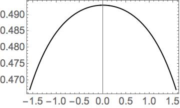
Figure 6: The function $f(\xi)$ in the needed range of its argument $\xi\in[-\pi/2,\pi/2]$

The components of the gauge potentials have the form Shuryak:2002qz

$$gA_{4}^{a}=-f(\xi){8t\rho x_{a}\over[(t-i\rho)^{2}-r^{2}][(t+i\rho)^{2}-r^{2}]}$$

$$gA^{a}_{i}=4\rho f(\xi){\delta_{ai}(t^{2}-r^{2}+\rho^{2})+2\rho\epsilon_{aij}x_{j}+2x_{i}x_{a}\over[(t-i\rho)^{2}-r^{2}][(t+i\rho)^{2}-r^{2}]}$$ (87)

which are manifestly real. From those potentials we have generated rather lengthy expressions for the electric and magnetic fields, and eventually for the CP-violating operators using Mathematica.

Let us only mention that for the sphaleron solution itself at $t=0$, the static solution is purely magnetic with $gA_{4}^{a}=0$. The magnetic field squared is spherically symmetric and simple

$$\vec{B}^{2}={96\rho^{4}\over(\rho^{2}+r^{2})^{4}}$$ (88)

We note that the specific expressions for pure-gauge sphaleron explosions were compared with numerical real-time simulations cold_scenario_simulations where they occur inside the “hot spots” with very good agreement Flambaum:2010fp . In the “cold scenario” numerically studied the sphaleron size was not determined by the Higgs VEV in the broken phase, but by the size of the hot spots with the unbroken phase. Unfortunately, a large size tail of the sphaleron distribution on which we focused in this work cannot be studied in similar simulations, as their probability is prohibitively low to reach it statistically.

Appendix C Sphalerons dominated by Higgs VEV

At $T$ somewhat below $T_{EW}$, when the Higgs VEV $v(T)$ is sufficiently developed, one may return to the original expressions developed by Klinkhamer and Manton Klinkhamer:1984di , modified from $T=0$ by using appropriate renormalized parameters. With two profile functions, $f(\xi),h(\xi)$ of normalized distance $\xi=gvr$, the sphaleron mass is given by the following integral

$$M={4\pi v\over g}\int_{0}^{\infty}d\xi\big{[}4(f^{\prime})^{2}+{8\over\xi^{2}}f^{2}(1-f)^{2}+{\xi^{2}\over 2}(h^{\prime})^{2}+h^{2}(1-f)^{2}+{\xi^{2}\over 4}{\lambda\over g^{2}}(h^{2}-1)^{2}\big{]}$$ (89)

The mass and size scales include temperature-dependent $v(T)$ which we took from the lattice simulation DOnofrio:2014rug

$${v(T)\over T}\approx 3\sqrt{1-{T\over T_{EW}}}$$ (90)

Renormalization of all Standard Model parameters at finite temperatures near $T_{EW}$ has been evaluated, via dimensional reduction, in the fundamental paper Kajantie:1995dw . From it, extrapolated to physical Higgs mass in vacuum, we extracted, at $T$ of interest, the following values of the coupling

$${\bar{\lambda}_{3}\over\bar{g}_{3}^{2}}\approx 0.22,\,\,\,\,\,\,\,\,\bar{g}_{3}^{2}\approx 0.39$$ (91)

and ignore their running in the temperature interval of interest.

For calculation we use the so called ansatz B of Klinkhamer:1984di with a single parameter $R$

$$f(\xi)={\xi^{2}\over R(R+4)},\,\,\,h(\xi)={\sigma R+1\over\sigma R+2}{\xi\over R},\,\,\,(\xi<R)$$ (92)

$$f(\xi)=1-{4\over R+4}e^{(R-\xi)/2},\,\,\,h(\xi)=1-{R\over\sigma R+2}{1\over\xi}e^{\sigma(R-\xi)},\,\,\,(\xi>R)$$ (93)

with $\sigma=\sqrt{2\cdot\lambda/g^{2}}$. These functions are plotted in Fig.7(a), which, among other features, show their continuity at $\xi=R$. Putting these profiles into the functional (89), one obtains the sphaleron mass $M(R)$. We also calculated r.m.s. radius of the sphaleron $\rho(R)$, defined by inserting extra $\xi^{2}$ into the energy density. In the main text we use $M(\rho)$ representation, with $R$ as a parameter.

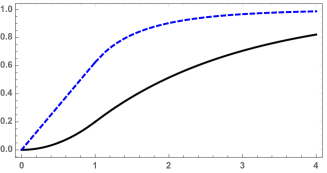
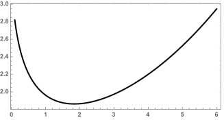
Figure 7: (a) The profile functions $f(\xi),h(\xi)$ versus $\xi$, for $R=1$, shown by black solid and blue dashed lines, respectively. (b) Root-mean-square size $\rho(R)$ as a function of parameter $R$.

Appendix D CP violation and differences of quark phases during quark production

The multiplication of four CKM matrices by propagators, containing additional phases induced by the quark mass terms in the Dirac operator, lead to the following expressions

$$\Delta P_{t}=2Je^{-i\phi_{c}-i\phi_{t}-i\phi_{u}}\big{(}e^{i\phi_{d}}-e^{i\phi_{s}}\big{)}(e^{i\phi_{c}}-e^{i\phi_{t}}\big{)}(e^{i\phi_{c}}-e^{i\phi_{u}}\big{)}(e^{i\phi_{t}}-e^{i\phi_{u}}\big{)}$$

$$\Delta P_{c}=2Je^{-i\phi_{c}-i\phi_{t}-i\phi_{u}}\big{(}e^{i\phi_{b}}-e^{i\phi_{d}}\big{)}(e^{i\phi_{c}}-e^{i\phi_{t}}\big{)}(e^{i\phi_{c}}-e^{i\phi_{u}}\big{)}(e^{i\phi_{t}}-e^{i\phi_{u}}\big{)}$$

$$\Delta P_{u}=2Je^{-i\phi_{c}-i\phi_{t}-i\phi_{u}}\big{(}e^{i\phi_{b}}-e^{i\phi_{s}}\big{)}(e^{i\phi_{c}}-e^{i\phi_{t}}\big{)}(e^{i\phi_{c}}-e^{i\phi_{u}}\big{)}(e^{i\phi_{t}}-e^{i\phi_{u}}\big{)}$$

$$\Delta P_{b}=2Je^{-i\phi_{c}-i\phi_{t}-i\phi_{u}}\big{(}e^{i\phi_{d}}-e^{i\phi_{s}}\big{)}(e^{i\phi_{c}}-e^{i\phi_{t}}\big{)}(e^{i\phi_{c}}-e^{i\phi_{u}}\big{)}(e^{i\phi_{t}}-e^{i\phi_{u}}\big{)}$$

$$\Delta P_{s}=2Je^{-i\phi_{c}-i\phi_{t}-i\phi_{u}}\big{(}e^{i\phi_{b}}-e^{i\phi_{d}}\big{)}(e^{i\phi_{c}}-e^{i\phi_{t}}\big{)}(e^{i\phi_{c}}-e^{i\phi_{u}}\big{)}(e^{i\phi_{t}}-e^{i\phi_{u}}\big{)}$$

$$\Delta P_{d}=2Je^{-i\phi_{c}-i\phi_{t}-i\phi_{u}}\big{(}e^{i\phi_{b}}-e^{i\phi_{s}}\big{)}(e^{i\phi_{t}}-e^{i\phi_{c}}\big{)}(e^{i\phi_{c}}-e^{i\phi_{u}}\big{)}(e^{i\phi_{t}}-e^{i\phi_{u}}\big{)}$$

with

$$J=cos(\theta_{12})cos(\theta_{13})^{2}cos(\theta_{23})sin(\theta_{12})sin(\theta_{13})sin(\theta_{23})sin(\delta)$$ (94)

The squared cos is not a misprint. The structure of these expressions is a reminder of the requirement that CP violation would vanish if any pair of masses is degenerate. Indeed, in this case we would be able to redefine the CKM matrix and eliminate the complex phase.

References

- (1) E. Witten, Phys. Rev. D 30, 272 (1984).
- (2) A. D. Sakharov, Pisma Zh. Eksp. Teor. Fiz. 5, 32 (1967) [JETP Lett. 5, 24 (1967)] [Sov. Phys. Usp. 34, 392 (1991)] [Usp. Fiz. Nauk 161, 61 (1991)].
- (3) K. Kajantie, M. Laine, K. Rummukainen and M. E. Shaposhnikov, Phys. Rev. Lett. 77, 2887 (1996) doi:10.1103/PhysRevLett.77.2887 [hep-ph/9605288].
- (4) C. Garcia-Recio and L. L. Salcedo, JHEP 0907, 015 (2009) [arXiv:0903.5494 [hep-ph]].
- (5) T. Brauner, O. Taanila, A. Tranberg and A. Vuorinen, JHEP 1211, 076 (2012) [arXiv:1208.5609 [hep-ph]].
- (6) V. V. Flambaum and E. Shuryak, Phys. Rev. D 82, 073019 (2010) [arXiv:1006.0249 [hep-ph]].
- (7) M. P. Crichigno, V. V. Flambaum, M. Y. Kuchiev and E. Shuryak, Phys. Rev. D 82, 073018 (2010) [arXiv:1006.0645 [hep-ph]].
- (8) Y. Burnier and E. Shuryak, Phys. Rev. D 84, 073003 (2011) [arXiv:1107.4060 [hep-ph]].
- (9) L. M. Krauss and M. Trodden, Phys. Rev. Lett. 83, 1502 (1999) [hep-ph/9902420].
- (10) J. Garcia-Bellido, D. Y. Grigoriev, A. Kusenko and M. E. Shaposhnikov, Phys. Rev. D 60, 123504 (1999) [hep-ph/9902449]; J. Garcia-Bellido, M. Garcia Perez and A. Gonzalez- Arroyo, Phys. Rev. D 67, 103501 (2003) [arXiv:hep- ph/0208228].
- (11) A. Tranberg and J. Smit, JHEP 0311, 016 (2003) [arXiv:hep-ph/0310342].; Jon-Ivar Skullerud, Jan Smit, Anders Tranberg, JHEP 08(2003)045; Meindert van der Meulen, Denes Sexty, Jan Smit, Anders Tranberg, JHEP 02(2006)029, hep-ph/0511080.
- (12) V. A. Kuzmin, V. A. Rubakov and M. E. Shaposhnikov, Phys. Lett. 155B, 36 (1985). doi:10.1016/0370-2693(85)91028-7
- (13) P. B. Arnold, D. Son and L. G. Yaffe, Phys. Rev. D 55, 6264 (1997) doi:10.1103/PhysRevD.55.6264 [hep-ph/9609481].
- (14) M. E. Shaposhnikov, Nucl. Phys. B 287, 757 (1987). doi:10.1016/0550-3213(87)90127-1
- (15) S. Y. Khlebnikov and M. E. Shaposhnikov, Nucl. Phys. B 308, 885 (1988). doi:10.1016/0550-3213(88)90133-2
- (16) M. D’Onofrio, K. Rummukainen and A. Tranberg, Phys. Rev. Lett. 113, no. 14, 141602 (2014) [arXiv:1404.3565 [hep-ph]].
- (17) F. R. Klinkhamer and N. S. Manton, Phys. Rev. D 30, 2212 (1984).
- (18) K. Kajantie, M. Laine, K. Rummukainen and M. E. Shaposhnikov, Nucl. Phys. B 458, 90 (1996) doi:10.1016/0550-3213(95)00549-8 [hep-ph/9508379].
- (19) T. Kalaydzhyan and E. Shuryak, Phys. Rev. D 91, no. 8, 083502 (2015) [arXiv:1412.5147 [hep-ph]].
- (20) Y. Brihaye, B. Kleihaus and J. Kunz, Phys. Rev. D 47, 1664 (1993).
- (21) U. M. Heller, F. Karsch and J. Rank, Nucl. Phys. Proc. Suppl. 63, 421 (1998) [hep-lat/9709065].
- (22) G. D. Moore, [hep-ph/0009161].
- (23) C. Jarlskog, Phys. Rev. Lett. 55, 1039 (1985).
- (24) A. M. Polyakov, Phys. Lett. 72B, 477 (1978).
- (25) D. M. Ostrovsky, G. W. Carter and E. V. Shuryak, Phys. Rev. D 66, 036004 (2002) [hep-ph/0204224].
- (26) E. Shuryak and I. Zahed, Phys. Rev. D 67, 014006 (2003) [hep-ph/0206022].
- (27) E. V. Shuryak, Sov. Phys. JETP 47, 212 (1978) [Zh. Eksp. Teor. Fiz. 74, 408 (1978)].
- (28) G. ’t Hooft, Phys. Rev. D 14, 3432 (1976) Erratum: [Phys. Rev. D 18, 2199 (1978)].
- (29) R. Rapp and E. V. Shuryak, Phys. Rev. Lett. 86, 2980 (2001) [hep-ph/0008326].
- (30) A. Hernandez, T. Konstandin and M. G. Schmidt, Nucl. Phys. B 812, 290 (2009) [arXiv:0810.4092 [hep-ph]].
- (31) Jan Smit,JHEP 0409 (2004) 067, hep-ph/0407161.
- (32) G. R. Farrar and M. E. Shaposhnikov, Phys. Rev. D 50, 774 (1994) [hep-ph/9305275].
- (33) M. B. Gavela, P. Hernandez, J. Orloff and O. Pene, Mod. Phys. Lett. A 9, 795 (1994) [hep-ph/9312215].
- (34) P. Huet and E. Sather, Phys. Rev. D 51, 379 (1995) [hep-ph/9404302].
- (35) R. N. Larsen, S. Sharma and E. Shuryak, Phys. Lett. B 794, 14 (2019) [arXiv:1811.07914 [hep-lat]].
- (36) J. Garcia-Bellido, M. Garcia-Perez and A. Gonzalez- Arroyo, Phys. Rev. D 69, 023504 (2004) [arXiv:hep- ph/0304285]. A. Tranberg and J. Smit, JHEP 0311, 016 (2003) [arXiv:hep-ph/0310342]. Jon-Ivar Skullerud, Jan Smit, Anders Tranberg, JHEP 08(2003)045.