Light axial-vector and vector resonances $X(2100)$ and $X(2239)$

Abstract

We study features of the resonances $X(2100)$ and $X(2239)$ by treating them as the axial-vector and vector tetraquarks with the quark content $ss\overline{s}\overline{s}$, respectively. The spectroscopic parameters of these exotic mesons are calculated in the framework of the QCD two-point sum rule method. Obtained prediction for the mass $m=(2067\pm 84)~{}\mathrm{MeV}$ of the axial-vector state is in excellent agreement with the mass of the structure $X(2100)$ recently observed by the BESIII Collaboration in the decay $J/\psi\to\phi\eta\eta^{\prime}$ as the resonance in the $\phi\eta^{\prime}$ mass spectrum. We explore also the $S$-wave decays $X(2100)\to\phi\eta^{\prime}$ and $X(2100)\to\phi\eta$ using the QCD light-cone sum rule approach and technical methods of the soft-meson approximation. The width of the axial-vector tetraquark, $\Gamma=(130.2\pm 30.1)~{}\mathrm{MeV}$, saturated by these two decays is comparable with the measured full width of the resonance $X(2100)$. Our prediction for the vector $ss\overline{s}\overline{s}$ tetraquark’s mass $\widetilde{m}=(2283\pm 114)~{}\mathrm{MeV}$ is consistent with the experimental result $2239.2\pm 7.1\pm 11.3~{}\mathrm{MeV}$ of the BESIII Collaboration for the mass of the resonance $X(2239)$.

I Introduction

Hadrons with exotic structures and/or quantum numbers, which differ them from the conventional $\bar{q}q$ mesons and $qq^{\prime}q^{\prime\prime}$ baryons were and remain in agenda of the High Energy Physics community. Properties of the ordinary hadrons, i.e. their spectroscopic parameters as well as their strong, semileptonic and radiative transitions have been investigated in the framework of Quantum Chromodynamics (QCD), and successfully confronted with available experimental data. In the nonperturbative regime of momentum transfers, the relevant theoretical results have been obtained using methods and phenomenological models which use either the first principles of QCD or invoke additional assumptions about the internal structure and dynamics of hadrons.

At the same time, the QCD allows existence of not only the ordinary hadrons but also particles built of four, five, or more quarks, quark-gluon hybrids, and glueballs. The idea about the multi-quark nature of some observed particles was first applied to explain the unusual features of the light scalar mesons with masses $m<1~{}\mathrm{GeV}$ Jaffe:1976ig . The reason is that the nonet of scalar particles in the standard model of mesons should be realized as $1{}^{3}P_{0}$ quark-antiquark states. But masses of these scalars, in accordance with various model computations, are higher than $1~{}\mathrm{GeV}$. Moreover, the standard model could not correctly describe the mass hierarchy of the mesons inside the nonet. These problems can be evaded by assuming that the light scalars are four-quark exotic mesons, or at least contain substantial four-quark component. In the context of this scheme low masses of the scalar mesons, as well as the hierarchy inside of the nonet receive natural explanations. A recent model of the both light and heavy scalar nonets is based on suggestion about diquark-antidiquark structure of these particles which are mixtures of the spin-$0$ diquarks from ($\overline{\mathbf{3}}_{c},\overline{\mathbf{3}}_{f}$) representation with spin-$1$ diquarks from ($\mathbf{6}_{c},\ \overline{\mathbf{3}}_{f})$ representation of the color-flavor group Kim:2017yvd . The spectroscopic parameters and width of the light scalar mesons $f_{0}(500)$ and $f_{0}(980)$ calculated by considering them as admixtures of the $SU_{f}(3)$ flavor octet and singlet tetraquarks are in a reasonable agreement with experimental data Agaev:2017cfz ; Agaev:2018sco . Other members of the light scalar nonet were also successfully explained as scalar particles with relevant diquark-antidiquark contents Agaev:2018fvz .

However, light quarks may not form stable tetraquarks: Theoretical studies proved that only tetraquarks composed of heavy and light diquarks may be stable against the strong decays. Thus, four-quark systems $QQ\bar{Q}\bar{Q}$ and $QQ\bar{q}\bar{q}$ were studied in Refs. Ader:1981db ; Lipkin:1986dw ; Zouzou:1986qh by employing the conventional potential model with additive pairwise interaction of color-octet exchange type. Within this approach it was demonstrated that states $QQ\bar{q}\bar{q}$ may form the stable composites provided that the ratio $m_{Q}/m_{q}$ is large enough. Experimental information on possible tetraquark candidates is also connected with the heavy resonances observed in various processes. Starting from discovery of the charmonium-like resonance $X(3872)$ by Belle Collaboration Choi:2003ue , the exotic mesons are the objects of rapidly growing studies. Valuable experimental data collected during years passed from observation of the $X(3872)$ resonance, as well as important theoretical achievements form now the physics of the exotic hadrons Chen:2016qju ; Chen:2016spr ; Esposito:2016noz ; Ali:2017jda ; Olsen:2017bmm .

There are only few resonances seen in the experiments which may be considered as four-quark systems containing only the light quarks. One of such states is the famous structure $Y(2175)$ discovered by the BaBar Collaboration in the process $e^{+}e^{-}\rightarrow\gamma_{\mathrm{ISR}}\phi f_{0}(980)$ as a resonance in the $\phi f_{0}(980)$ invariant mass spectrum Aubert:2006bu . Existence of the $Y(2175)$ later was confirmed by the BESII, Belle, and BESIII collaborations as well Ablikim:2007ab ; Shen:2009zze ; Ablikim:2014pfc . The mass and width of this state with spin-parities $J^{PC}=1^{--}$ is $m=2175\pm 10\pm 15~{}\mathrm{MeV}$ and $\Gamma=58\pm 16\pm 20~{}\mathrm{MeV}$, respectively.

Other resonances which may be interpreted as light exotic mesons were observed recently by the BESIII Collaboration. Thus, the $X(2239)$ was seen in the process $e^{+}e^{-}\rightarrow K^{+}K^{-}$ as a resonant structure in the cross section shape line Ablikim:2018iyx . The mass and width of this state were found equal to $m=2239.2\pm 7.1\pm 11.3~{}\mathrm{MeV}$ and $\Gamma=139.8\pm 12.3\pm 20.6~{}\mathrm{MeV}$, respectively. The $X(2100)$ was fixed in the process $J/\psi\rightarrow\phi\eta\eta^{\prime}$ as a resonance in the $\phi\eta^{\prime}$ mass spectrum Ablikim:2018xuz . The collaboration studied the angular distribution of $J/\psi\rightarrow X(2100)\eta$ , but due to limited statistics could not clearly distinguish $1^{+}$ or $1^{-}$ assumption for the spin-parity $J^{P}$ of the $X(2100)$.  Therefore, the spectroscopic parameters of this resonance were determined using both of these assumptions. In the case $J^{P}=1^{-}$  the mass and width of the $X(2100)$ were measured to be $m=2002.1\pm 27.5\pm 21.4~{}\mathrm{MeV}$ and $\Gamma=129\pm 17\pm 9~{}\mathrm{MeV}$. Alternatively, the assumption $J^{P}=1^{+}$ led to the results $m=2062.8\pm 13.1\pm 7.2~{}\mathrm{MeV}$ and $\Gamma=177\pm 36\pm 35~{}\mathrm{MeV}$.

Theoretical interpretations of these light resonances which may be considered as candidates for tetraquarks, as usua,l comprise all possible models and approaches available in high energy physics. Because the $Y(2175)$ was discovered more than ten years ago, there are numerous and diverse articles in the literature devoted to its investigation. There are quite natural attempts to interpret it as an $2{}^{3}D_{1}$ excitation of the conventional $\overline{s}s$ meson Ding:2007pc ; Wang:2012wa . Another traditional approach is to treat such states as dynamically generated resonances. As a dynamically generated state in the $\phi K\overline{K}$ system, the $Y(2175)$ was examined in Ref. MartinezTorres:2008gy . The similar dynamical picture may appear due to self-interaction between $\phi$ and $f_{0}(980)$ mesons as well AlvarezRuso:2009xn . Alternative explanations of the $Y(2175)$ resonance’s structure include a hybrid meson $\overline{s}sg$, or a baryon-antibaryon $qqs\overline{q}\overline{q}\overline{s}$ state that couples strongly to the $\Lambda\overline{\Lambda}$ channel (for relevant references and other models, see Ref. Ablikim:2018iyx ).

The resonance $Y(2175)$ as a vector tetraquark with $s\overline{s}s\overline{s}$ or $ss\overline{s}\overline{s}$ content was explored in Refs. Wang:2006ri and Chen:2008ej ; Chen:2018kuu , respectively. In these works the authors used the QCD sum rule method and evaluated spectroscopic parameters of these states. The newly found structures $X(2100)$ and $X(2239)$ (hereafter $X_{1}$ and $X_{2}$, respectively) were also analyzed as vector or axial-vector tetraquarks. Thus, in Ref. Lu:2019ira the mass spectrum of the $ss\overline{s}\overline{s}$ tetraquark states was investigated within the relativized quark model. The authors concluded that the resonance $X_{2}$ can be assigned as a $P$-wave $1^{--}$ $ss\overline{s}\overline{s}$ tetraquark. In the framework of the QCD sum rule method the $X_{1}$ resonance was studied in Refs. Cui:2019roq ; Wang:2019nln . Predictions obtained there allowed the authors to interpret it as the axial-vector $ss\overline{s}\overline{s}$ tetraquark with the quantum numbers $J^{PC}=1^{+-}$. In accordance with Ref. Wang:2019qyy , the $X_{1}$ may be identified as the second radial excitation of the conventional meson $h_{1}(1380)$.

As is seen, theoretical interpretations of observed light resonances are numerous and sometimes contradict to each other. There is a necessity to consider this problem in a more detailed form and analyze not only spectroscopic parameters of the light resonances, but also to explore their decay channels and widths. In the present work we study the axial-vector and vector light tetraquarks $ss\overline{s}\overline{s}$ and compute their masses and couplings. By confronting theoretical predictions and experimental data we identify the observed resonances $Y(2175)$, $X_{1}$ and $X_{2}$ with these tetraquark structures. It turns out that the resonance $X_{1}$ can be interpreted as a axial-vector tetraquark state. We calculate the width of the decays $X_{1}\rightarrow\phi\eta^{\prime}$ and $X_{1}\rightarrow\phi\eta$ which are essential for our interpretation of the $X_{1}$. Among the vector resonances $Y(2175)$ and $X_{2}$, parameters of the latter is closer to our result.

Calculations in the present paper are performed in the context of the QCD sum rule method, which is one of the powerful nonperturbative approaches in high energy physics Shifman1 ; Shifman2 . The masses and couplings of the four-quark systems are evaluated using two-point QCD sum rules with an accuracy higher than in existing samples. To find the width of the decays $X_{1}\rightarrow\phi\eta^{\prime}$ and $X_{1}\rightarrow\phi\eta$ we employ sum rules on the light cone and technical tools of the soft-meson approximation Balitsky:1989ry ; Belyaev:1994zk .

This paper is structured in the following form: In Sections II and III we analyze the spectroscopic parameters of the axial-vector and vector tetraquarks $ss\overline{s}\overline{s}$ and provide details of relevant sum rule calculations. In Sec. IV the strong couplings $g_{X_{1}\phi\eta^{\prime}}$ and $g_{X_{1}\phi\eta}$ corresponding to the vertices $X_{1}\phi\eta^{\prime}$ and $X_{1}\phi\eta$ are found using the QCD light-cone sum rule method. These coupling are required to evaluate the width of the decays $X_{1}\rightarrow\phi\eta^{\prime}$ and $X_{1}\rightarrow\phi\eta$, respectively. Section V contains summary of the obtained results and our conclusions.

II Mass and coupling of the axial-vector tetraquark $ss\overline{s}\overline{s}$

In this section we compute the mass and coupling of the axial-vector tetraquark $T_{\mathrm{AV}}=ss\overline{s}\overline{s}$. As it has been emphasized above, to this end we use the QCD sum rules method which is based on first principles of QCD and allows one, via a quark-hadron duality assumption, to express physical parameters of hadrons in terms of the universal nonperturbative quantities, i.e. vacuum expectation values of local quark, gluon, and mixed operators. This method was successfully applied to explore parameters not only of conventional hadrons, but also to study various multi-quark systems Albuquerque:2018jkn .

To derive the required sum rules we consider the two-point correlation function $\Pi_{\mu\nu}(p)$, which is defined by the formula

$$\Pi_{\mu\nu}(p)=i\int d^{4}xe^{ipx}\langle 0|\mathcal{T}\{J_{\mu}(x)J_{\nu}^{{\dagger}}(0)\}|0\rangle,$$ (1)

where $J_{\mu}(x)$ is the interpolating current for the axial-vector tetraquark $ss\overline{s}\overline{s}$. The choice of $J_{\mu}(x)$ in one of the main operations in the sum rule computations. The tetraquark with content $ss\overline{s}\overline{s}$ and spin-parities $J^{PC}=1^{+-}$ can be interpolated using different currents. The current that leads to a reliable prediction for the mass and coupling of the axial-vector state has the following form Cui:2019roq

$$J_{\mu}(x)=\left[s_{a}^{T}(x)C\gamma^{\nu}s_{b}(x)\right]\left[\overline{s}_{a}(x)\sigma_{\mu\nu}\gamma_{5}C\overline{s}_{b}^{T}(x)\right]$$

$$-\left[s_{a}^{T}(x)C\sigma_{\mu\nu}\gamma_{5}s_{b}(x)\right]\left[\overline{s}_{a}(x)\gamma^{\nu}C\overline{s}_{b}^{T}(x)\right].$$ (2)

Here $a$ and $b$ are the color indices and $C$ is the charge conjugation operator.

The sum rules necessary to calculate the mass $m$ and coupling $f$ of the $T_{\mathrm{AV}}$ can be derived in accordance with prescriptions of the method, which require first to express the correlation function $\Pi_{\mu\nu}(p)$ using the tetraquark’s physical parameters . We consider $T_{\mathrm{AV}}$ as a ground-state particle, and after isolating the first term in $\Pi_{\mu\nu}^{\mathrm{Phys}}(p)$ get

$$\Pi_{\mu\nu}^{\mathrm{Phys}}(p)=\frac{\langle 0|J_{\mu}|T_{\mathrm{AV}}(p)\rangle\langle T_{\mathrm{AV}}(p)|J_{\nu}^{\dagger}|0\rangle}{m^{2}-p^{2}}+\dots$$ (3)

Equation (3) is obtained by saturating the correlation function with a complete set of $J^{P}=1^{+-}$ states and carrying out the integration over $x$. Effects of higher resonances and continuum states are denoted above by dots.

To simplify further the correlator $\Pi_{\mu\nu}^{\mathrm{Phys}}(p)$, it is convenient to introduce the matrix element

$$\langle 0|J_{\mu}|T_{\mathrm{AV}}(p,\epsilon)\rangle=fm\epsilon_{\mu},$$ (4)

where $\epsilon_{\mu}$ is the polarization vector of the $T_{\mathrm{AV}}$ state. Then the correlation function $\Pi_{\mu\nu}^{\mathrm{Phys}}(p)$ takes the simple form

$$\Pi_{\mu\nu}^{\mathrm{Phys}}(p)=\frac{m^{2}f^{2}}{m^{2}-p^{2}}\left(-g_{\mu\nu}+\frac{p_{\mu}p_{\nu}}{m^{2}}\right)+\ldots$$ (5)

Equation (5) determines the physical or phenomenological side of the sum rules.

The correlation function $\Pi_{\mu\nu}(p)$ calculated by employing the quark propagators constitutes the QCD side of the sum rules. It is given by the expression

$$\Pi_{\mu\nu}^{\mathrm{OPE}}(p)=\frac{i}{4}\int d^{4}xe^{ipx}\left\{\mathrm{Tr}\left[\gamma^{\alpha}\widetilde{S}^{a^{\prime}b}(-x)\gamma^{\beta}S^{b^{\prime}a}(-x)\right]\right.$$

$$\times\mathrm{Tr}\left[S^{ab^{\prime}}(x)\gamma_{\nu}\gamma_{\beta}\gamma_{5}\widetilde{S}^{ba^{\prime}}(x)\gamma_{5}\gamma_{\mu}\gamma_{\alpha}\right]-\mathrm{Tr}\left[\gamma^{\alpha}\widetilde{S}^{bb^{\prime}}(-x)\right.$$

$$\left.\times\gamma^{\beta}S^{a^{\prime}a}(-x)\right]\mathrm{Tr}\left[S^{ab^{\prime}}(x)\gamma_{\nu}\gamma_{\beta}\gamma_{5}\widetilde{S}^{ba^{\prime}}(x)\gamma_{5}\gamma_{\mu}\gamma_{\alpha}\right]$$

$$\left.+62\ \mathrm{similar\ terms}\right\},$$ (6)

where $S^{ab}(x)$ is the $s$-quark propagator and

$$\widetilde{S}(x)=CS^{T}(x)C.$$ (7)

In calculations we employ the $x$-space light-quark propagator

$$S^{ab}(x)=i\frac{\not{x}}{2\pi^{2}x^{4}}\delta_{ab}-\frac{m_{s}}{4\pi^{2}x^{2}}\delta_{ab}-\frac{\langle\overline{s}s\rangle}{12}\left(1-i\frac{m_{s}}{4}\not{x}\right)\delta_{ab}$$

$$-\frac{x^{2}}{192}\langle\overline{s}g_{s}\sigma Gs\rangle\left(1-i\frac{m_{s}}{6}\not{x}\right)\delta_{ab}$$

$$-\frac{ig_{s}G_{ab}^{\mu\nu}}{32\pi^{2}x^{2}}\left[\not{x}\sigma_{\mu\nu}+\sigma_{\mu\nu}\not{x}\right]-\frac{\not{x}x^{2}g_{s}^{2}}{7776}\langle\overline{s}s\rangle^{2}\delta_{ab}$$

$$-\frac{x^{4}\langle\overline{s}s\rangle\langle g_{s}^{2}G^{2}\rangle}{27648}\delta_{ab}+\frac{m_{s}g_{s}}{32\pi^{2}}G_{ab}^{\mu\nu}\sigma_{\mu\nu}\left[\ln\left(\frac{-x^{2}\Lambda^{2}}{4}\right)+2\gamma_{E}\right]$$

$$+\cdots,$$ (8)

where $\gamma_{E}\simeq 0.577$ is the Euler constant, and $\Lambda$ is the QCD scale parameter. We use also the notation $G_{ab}^{\mu\nu}\equiv G_{A}^{\mu\nu}t_{ab}^{A},\ A=1,2,\ldots 8$, and $t^{A}=\lambda^{A}/2$, with $\lambda^{A}$ being the Gell-Mann matrices.

The propagator (8) contains various light quark, gluon and mixed condensates of different dimensions. The term $\langle\overline{s}g_{s}\sigma Gs\rangle$ written down in Eq. (8) as well as other ones proportional to $\langle\overline{s}s\rangle^{2}$, and $\langle\overline{s}s\rangle\langle g_{s}^{2}G^{2}\rangle$ are obtained using the factorization hypothesis of the higher dimensional condensates. It is known, however, that the factorization assumption is not precise and violates is the case of higher dimensional condensates Ioffe:2005ym . Thus, for the condensates of dimension 10 even an order of magnitude of such a violation is unclear. But, contributions to sum rules arising from higher dimensional condensates are very small, therefore, in what follows, we ignore uncertainties generated by this violation.

At the next stage we calculate the resultant four-$x$ Fourier integrals in $\Pi_{\mu\nu}^{\mathrm{OPE}}(p)$. The correlation function $\Pi_{\mu\nu}^{\mathrm{OPE}}(p)$ obtained by this way contains two Lorentz structures which may be chosen to derive the sum rules. For our purposes terms $\sim g_{\mu\nu}$ both in $\Pi_{\mu\nu}^{\mathrm{Phys}}(p)$ and $\Pi_{\mu\nu}^{\mathrm{OPE}}(p)$ are convenient, because scalar particles do not contribute to these terms. Afterwards we equate the corresponding invariant amplitudes $\Pi^{\mathrm{Phys}}(p^{2})$ and $\Pi^{\mathrm{OPE}}(p^{2})$, and find an expression in momentum space which, after some manipulations, can be used to derive the desired sum rules. Indeed, to suppress contributions of the higher resonances and continuum states we apply to both sides of the obtained equality the Borel transformation. The last operation to be carried out is continuum subtraction, which is achieved by invoking assumption on quark-hadron duality. After these manipulations the equality depends on auxiliary parameters of the sum rules $M^{2}$ and $s_{0}$: $M^{2}$ is the Borel parameter appeared due to corresponding transformation, $s_{0}$ is the continuum subtraction parameter that separates the ground-state and higher resonances from each another.

To find the sum rules for $m$ and $f$ we need an additional expression which can be obtained by acting $d/d\left(-1/M^{2}\right)$ to the first equality. The sum rules for $m$ and $f$ have the perturbative and nonperturbative components. The nonperturbative components contain the quark, gluon, and mixed vacuum condensates, which appears after sandwiching relevant terms in $\Pi^{\mathrm{OPE}}(p)$ between vacuum states. Our analytical results contain the nonperturbative terms up to dimension-20. We keep all of them in numerical computations bearing in mind that higher dimensional terms appear due to the factorization hypothesis as product of basic condensates, and do not encompass all dimension-20 contributions.

In numerical computations we utilize the following quark and mixed condensates: $\langle\bar{s}s\rangle=-0.8\times(0.24\pm 0.01)^{3}~{}\mathrm{GeV}^{3}$ and $\langle\overline{s}g_{s}\sigma Gs\rangle=m_{0}^{2}\langle\bar{s}s\rangle$, where $m_{0}^{2}=(0.8\pm 0.1)~{}\mathrm{GeV}^{2}$. An important ingredient of analyses is the gluon condensate $\ \langle\alpha_{s}G^{2}/\pi\rangle=(0.012\pm 0.004)~{}\mathrm{GeV}^{4}$. Our sum rules depend on the strange quark mass for which we use its value $m_{s}=93_{-5}^{+11}~{}\mathrm{MeV}$ borrowed from Ref. Tanabashi:2018oca .  The scale parameter $\Lambda$ can be chosen within the limits $(0.5,\ 1)\ \mathrm{GeV}$; we utilize the central value $\Lambda=0.75\ \mathrm{GeV}$.

A very important problem of calculations is a proper choice for the Borel $M^{2}$ and continuum threshold $s_{0}$ parameters. These parameters are not arbitrary, but should meet some known requirements: At maximum of the Borel parameter the pole contribution ($\mathrm{PC}$) has to constitute a fixed part of the correlation function, whereas at minimum of $M^{2}$ it must be a dominant contribution. We define $\mathrm{PC}$ in the form

$$\mathrm{PC}=\frac{\Pi(M^{2},s_{0})}{\Pi(M^{2},\infty)},$$ (9)

where $\Pi(M^{2},s_{0})$ is the Borel transformed and subtracted invariant amplitude $\Pi^{\mathrm{OPE}}(p^{2})$. The minimum of $M^{2}$ is fixed from convergence of the sum rules, i.e. at $M_{\mathrm{min}}^{2}$ contribution of the last term (or a sum of last few terms) cannot exceed, for example, $0.01$ part of the whole result. In the case of multi-quark hadrons at $M_{\mathrm{max}}^{2}$ one, as usual, requires $\mathrm{PC}>0.2$. There is an another restriction on the lower limit $M_{\mathrm{min}}^{2}$: at $M_{\mathrm{min}}^{2}$ the perturbative contribution has to prevail over the nonperturbative one.

The sum rule predictions should not depend on the parameters $M^{2}$ and $s_{0}$. But in real calculations $m$ and $f$ demonstrate sensitiveness to the choice of $M^{2}$ and $s_{0}$. Hence, the parameters $M^{2}$ and $s_{0}$ have to be fixed in such a manner that to reduce this effect to a minimum. Performed analysis allows us to find the working regions

$$M^{2}\in[1.4,\ 2]~{}\mathrm{GeV}^{2},\ s_{0}\in[6,\ 7]~{}\mathrm{GeV}^{2},$$ (10)

which obey all the aforementioned constraints.

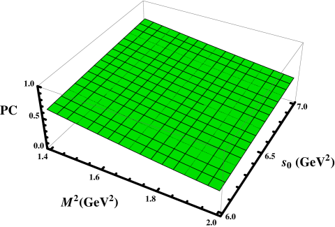
Figure 1: Dependence of the pole contribution on $M^{2}$ and $s_{0}$.

In Fig. 1 we depict the pole contribution as functions of $M^{2}$ and $s_{0}$: at $M^{2}=1.4$ the pole contribution is $0.68$, whereas at $M^{2}=2$ it becomes equal to $0.39$. The prediction for the mass $m$ is plotted in Fig. 2, where one can see its weak dependence on the parameters $M^{2}$ and $s_{0}$. The results for the spectroscopic parameters of the tetraquark $T_{\mathrm{AV}}$ read:

$$m = \left(2067\pm 84\right)~{}\mathrm{MeV},\$$

$$f = \left(0.89\pm 0.11\right)\times 10^{-2}~{}\mathrm{GeV}^{4}.$$ (11)

Theoretical errors in the sum rule computations appear due to different sources. The auxiliary parameters $M^{2}$ and $s_{0}$ are main sources of these ambiguities. Errors connected with uncertainies of $m_{s}$ and vacuum condensates are not substantial. For example, varying $m_{s}$ within tle limits $88~{}\mathrm{MeV}\leq m_{s}\leq 104~{}\mathrm{MeV}\$leads to corrections $\binom{+2~{}}{-1}~{}\mathrm{MeV}$ for $m$ and $\binom{+0.0002}{-0.0001}$ $~{}\mathrm{GeV}^{4}$ for $f$.  All of these errors are taken into account in (11).

The result obtained for the mass of the axial-vector tetraquark $T_{\mathrm{AV}}$ is in excellent agreement with the mass of the structure $X_{1}$ reported by the BESIII Collaboration. Therefore, it is possible to identify $T_{\mathrm{AV}}$ with the resonance $X_{1}$. Our conclusion is also in accord with previous theoretical predictions obtained by means of the QCD sum rules method. Thus, the mass of the resonance $X_{1}$ was estimated in Refs. Cui:2019roq ; Wang:2019nln

$$m=2000_{-90}^{+100}~{}\mathrm{MeV},\ m=\left(2080\pm 120\right)~{}\mathrm{MeV},$$ (12)

respectively. As is seen, all these calculations support the assumption on the axial-vector tetraquark nature of the structure $X_{1}$. But one needs to explore its decay channels $X_{1}\rightarrow\phi\eta^{\prime}$ and $X_{1}\rightarrow\phi\eta$, and find width of this resonance: only after successful comparison with experimental data it is legitimate to make more strong conclusion about $X_{1}$. We are going to address this problem in Sec. IV.

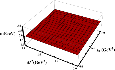
Figure 2: The mass of the tetraquark $T_{\mathrm{AV}}$ as a function of the Borel and continuum threshold parameters.

III Spectroscopic parameters of the vector tetraquark $ss\overline{s}\overline{s}$

In the previous section we have explored the axial-vector tetraquark $T_{\mathrm{AV}}$ and identified it as a candidate for the resonance $X_{1}$. But there are two other light states which should be classified within the four-quark picture. In the present section we are going to analyze the vector tetraquark $T_{\mathrm{V}}=ss\overline{s}\overline{s}$ with the quantum numbers $J^{PC}=1^{--}$ and compare the obtained result for its mass with the experimental information of BaBar and BESIII collaborations.

Calculations of the $T_{\mathrm{V}}$ tetraquark’s mass $\widetilde{m}$ and coupling $\widetilde{f}$ do not differ considerably from ones fulfilled in the previous section. There are only some qualitative differences on which we want to concentrate. First of all, the interpolating current for the vector state is defined by the expression Chen:2018kuu

$$\widetilde{J}_{\mu}(x)=\left[s_{a}^{T}(x)C\gamma_{5}s_{b}(x)\right]\left[\overline{s}_{a}(x)\gamma_{\mu}\gamma_{5}C\overline{s}_{b}^{T}(x)\right]$$

$$-\left[s_{a}^{T}(x)C\gamma_{\mu}\gamma_{5}s_{b}(x)\right]\left[\overline{s}_{a}(x)\gamma_{5}C\overline{s}_{b}^{T}(x)\right].$$ (13)

The physical side of the sum rule is given by Eq. (5) with evident replacements. The correlation function $\widetilde{\Pi}_{\mu\nu}^{\mathrm{OPE}}(p)$ that determines the QCD side of the sum rule has the following expression

$$\widetilde{\Pi}_{\mu\nu}^{\mathrm{OPE}}(p)=i\int d^{4}xe^{ipx}\left\{\mathrm{Tr}\left[\gamma_{5}\widetilde{S}^{b^{\prime}b}(-x)\gamma_{5}\gamma_{\nu}S^{a^{\prime}a}(-x)\right]\right.$$

$$\times\mathrm{Tr}\left[S^{aa^{\prime}}(x)\gamma_{5}\widetilde{S}^{bb^{\prime}}(x)\gamma_{5}\gamma_{\mu}\right]-\mathrm{Tr}\left[\gamma_{5}\widetilde{S}^{a^{\prime}b}(-x)\gamma_{\nu}\right.$$

$$\left.\times\gamma_{5}S^{b^{\prime}a}(-x)\right]\mathrm{Tr}\left[S^{aa^{\prime}}(x)\gamma_{5}\widetilde{S}^{bb^{\prime}}(x)\gamma_{5}\gamma_{\mu}\right]$$

$$\left.+14\ \mathrm{similar\ terms}\right\},$$ (14)

The remaining operations have been explained above. Therefore we present only final results of performed analysis. The working windows for the Borel and continuum threshold parameters in the case of the vector tetraquark $T_{\mathrm{V}}$ are determined by the intervals

$$M^{2}\in[1.4,\ 2]~{}\mathrm{GeV}^{2},\ s_{0}\in[7,\ 8]~{}\mathrm{GeV}^{2}.$$ (15)

It is seen that these regions differ from ones presented in Eq. (10) by only small shift of the parameter $s_{0}$. The windows (10) comply all constraints necessary in the sum rule computations. In fact, at $M^{2}=1.4$ the pole contribution is $60\%$, whereas at $M^{2}=2$ it is equal to $30\%$ of the whole result. Convergence of the sum rules is also satisfied. The mass and coupling of the vector tetraquark $T_{\mathrm{V}}$ are:

$$\widetilde{m} = \left(2283\pm 114\right)~{}\mathrm{MeV},\$$

$$\widetilde{f} = \left(0.57\pm 0.10\right)\times 10^{-2}~{}\mathrm{GeV}^{4}.$$ (16)

In Fig. 3 we plot the spectroscopic parameters $\widetilde{m}$ and $\widetilde{f}$ as functions of $M^{2}$ and $s_{0}$.

Comparing the mass of the vector state $T_{\mathrm{V}}$ and experimental information on the resonances $Y(2175)$ and $X_{2}$, one can see that it can be identified with the $X_{2}$. In fact, difference between the masses of $T_{\mathrm{V}}$ and $X_{2}$ is approximately $60~{}\mathrm{MeV}$ smaller than between $T_{\mathrm{V}}$ and $Y(2175)$. The similar conclusion was drawn also in Ref. Lu:2019ira . The mass $m_{X_{2}}=2227~{}\mathrm{MeV}$ of the four-quark vector system $ss\overline{s}\overline{s}$ found there is consistent with BESIII data.

The mass of the vector tetraquark $ss\overline{s}\overline{s}$ was computed using the QCD sum rule method in Refs. Wang:2019nln and Chen:2018kuu as well. The prediction for the mass of this four-quark meson $m=(3080\pm 110)~{}\mathrm{MeV}$ made in Refs. Wang:2019nln disfavors classifying it as the resonance $Y(2175)$. Comparing this result with recent measurements of the BESIII Collaboration, we see that it also cannot be assigned to be the resonance $X_{2}$. To study vector tetraquarks with the $ss\overline{s}\overline{s}$ content, in Ref. Chen:2018kuu the authors constructed two independent interpolating currents which couple to $J^{PC}=1^{--\text{ }}$states. These currents led to slightly different predictions $m_{1}=(2410\pm 250)~{}\mathrm{MeV}$ and $m_{2}=(2340\pm 170)~{}\mathrm{MeV}$. In accordance with Chen:2018kuu the first state might correspond to a structure in the $\phi f_{0}(980)$ invariant mass spectrum at around $2.4~{}\mathrm{GeV}$. The second one was interpreted in Ref. Chen:2018kuu as the resonance $Y(2175)$ but, from our point of view, it is closer to the structure $X_{2}$.

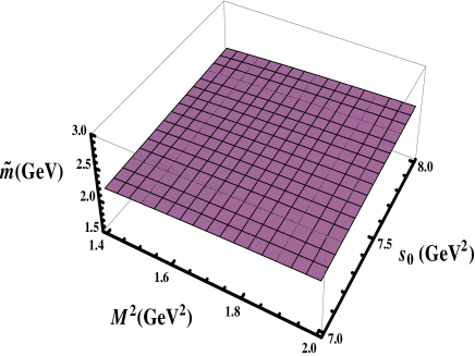
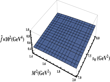
Figure 3: The mass (left panel) and coupling (right panel) of the vector tetraquark $T_{\mathrm{V}}$ as functions of the Borel and continuum threshold parameters.

IV Decays $X_{1}\rightarrow\phi\eta^{\prime}$ and $X_{1}\rightarrow\phi\eta$

Within the framework of the QCD sum rule method the decay $X_{1}\rightarrow\phi\eta^{\prime}$ [and $X_{1}\rightarrow\phi\eta$] can be investigated by means of different approaches. In fact, a key quantity to calculate the width of this decay is the coupling $g_{X_{1}\phi\eta^{\prime}}$ describing the strong interaction in the vertex $X_{1}\phi\eta^{\prime}$. The coupling $g_{X_{1}\phi\eta^{\prime}}$ can be evaluated using, for example, the QCD three-point sum rule method. Alternatively, one can extract it from the relevant QCD light-cone sum rule (LCSR), which has some advantages when calculating tetraquark-meson-meson vertices containing light mesons. The reason is that the LCSRs for tetraquark-meson-meson vertices differ from ones involving only conventional mesons. Thus, the LCSR for vertices of conventional mesons depends on various distribution amplitudes (DAs) of one of the final mesons, which encode all information about nonperturbative dynamical properties of the meson. In the case of the tetraquark-meson-meson vertices due to four-quark nature of the tetraquark, after contracting relevant quark fields instead of DAs of a the final meson the sum rule contains only local matrix elements of this meson. Then to satisfy the four-momentum conservation at vertices the momentum of a final light meson should be set $q=0$. This leads to crucial changes in the calculational scheme, because now one has to accompany the LCSR method with technical tools of the soft-meson approximation Belyaev:1994zk ; Agaev:2016dev .

Let us consider the dominant process $X_{1}\rightarrow\phi\eta^{\prime}$ in a detailed form. The second decay mode $X_{1}\rightarrow\phi\eta$ , as we shall see below, can be analyzed in the same manner. The starting point to explore the decay $X_{1}\rightarrow\phi\eta^{\prime}$ is the correlation function

$$\widehat{\Pi}_{\mu\nu}(p,q)=i\int d^{4}xe^{ipx}\langle\eta^{\prime}(q)|\mathcal{T}\{J_{\mu}^{\phi}(x)J_{\nu}^{\dagger}(0)\}|0\rangle,$$ (17)

where $J_{\mu}^{\phi}(x)$ is the interpolating current of the $\phi$ meson

$$J_{\mu}^{\phi}(x)=i\overline{s}_{i}(x)\gamma_{\nu}s_{i}(x).$$ (18)

Following the standard recipes, we write down $\widehat{\Pi}_{\mu\nu}(p,q)$ in terms of the physical parameters of the particles $X_{1},\ \phi$ and $\eta^{\prime}$

$$\widehat{\Pi}_{\mu\nu}^{\mathrm{Phys}}(p,q)=\frac{\langle 0|J_{\mu}^{\phi}(x)|\phi(p)\rangle}{p^{2}-m_{\phi}^{2}}\langle\phi(p)\eta^{\prime}(q)|X_{1}(p^{\prime})\rangle$$

$$\times\frac{\langle X_{1}(p^{\prime})|J_{\nu}^{\dagger}|0\rangle}{p^{\prime 2}-m^{2}}+...,$$ (19)

where $p^{\prime}$ and $p$, $q$ are momenta of the initial and final particles, respectively. In Eq. (19) contributions of excited resonances and continuum states are indicated by dots. By utilizing the matrix elements

$$\langle 0|J_{\mu}^{\phi}(x)|\phi(p)\rangle=f_{\phi}m_{\phi}\varepsilon_{\mu},$$

$$\langle\phi(p)\eta^{\prime}(q)|X_{1}(p^{\prime})\rangle=g_{X_{1}\phi\eta^{\prime}}\left[(p\cdot p^{\prime})(\varepsilon^{\ast}\cdot\varepsilon^{\prime})\right.$$

$$\left.-(p\cdot\varepsilon^{\prime})(p^{\prime}\cdot\varepsilon^{\ast})\right],$$ (20)

one can considerably simplify $\widehat{\Pi}_{\mu\nu}^{\mathrm{Phys}}(p,q)$. The matrix element $\langle 0|J_{\mu}^{\phi}(x)|\phi(p)\rangle$ is expressed in terms of $\phi$ meson’s mass $m_{\phi}$ , decay constant $f_{\phi}$ and polarization vector $\varepsilon_{\mu}$. The matrix element of the vertex $X_{1}\phi\eta^{\prime}$ is written down using the strong coupling $g_{X_{1}\phi\eta^{\prime}}$ which has to be evaluated from the sum rule. In the soft limit $q\rightarrow 0$ we get $p^{\prime}=p$, as a result instead of two-variable Borel transformation we have to perform one-variable Borel transformation, which yields

$$\mathcal{B}\widehat{\Pi}_{\mu\nu}^{\mathrm{Phys}}(p)=g_{X_{1}\phi\eta^{\prime}}m_{\phi}mf_{\phi}f\frac{e^{-\overline{m}^{2}/M^{2}}}{M^{2}}$$

$$\times\left(\overline{m}^{2}g_{\mu\nu}-p_{\nu}p_{\mu}^{\prime}\right)+\ldots,$$ (21)

where $\overline{m}^{2}=(m_{\phi}^{2}+m^{2})/2.$ In Eq. (21) we still keep $p_{\nu}\neq p_{\mu}^{\prime}$ to make clear the Lorentz structure of the obtained expression. To derive the LCSR for the strong coupling $g_{X_{1}\phi\eta^{\prime}}$ we will employ the structure $\sim g_{\mu\nu}$.

In the soft approximation the physical side of the sum rule has more complicated structure than in the case of full LCSR method. The complications are connected with behavior of contributions arising from higher resonances and continuum states in the soft limit. The problem is that in the soft limit some of these contributions even after the Borel transformation remain unsuppressed and appear as contaminations in the physical side Belyaev:1994zk . Therefore, before performing the continuum subtraction in the final sum rule they should be removed by means of some operations. This problem is solved by acting on the physical side of sum rule by the operator Belyaev:1994zk ; Ioffe:1983ju

$$\mathcal{P}(M^{2},\overline{m}^{2})=\left(1-M^{2}\frac{d}{dM^{2}}\right)M^{2}e^{\overline{m}^{2}/M^{2}},$$

that singles out the ground-state term. It is natural that the same operator $\mathcal{P}(M^{2},\overline{m}^{2})$ should be applied also to the QCD side of the sum rule. But before these manipulations the correlation function $\widehat{\Pi}_{\mu\nu}^{\mathrm{OPE}}(p,q)$ has to be calculated in the soft-meson approximation and expressed in terms of the $\eta^{\prime}$ meson’s local matrix elements.

In the soft limit $\widehat{\Pi}_{\mu\nu}^{\mathrm{OPE}}(p)$ is given by the formula

$$\widehat{\Pi}_{\mu\nu}^{\mathrm{OPE}}(p)=2i\int d^{4}xe^{ipx}\left\{\left[\sigma_{\mu\rho}\gamma_{5}\widetilde{S}^{ib}(x){}\gamma_{\nu}\widetilde{S}^{bi}(-x)\gamma^{\rho}\right.\right.$$

$$\left.-\gamma^{\rho}\widetilde{S}^{ib}(x){}\gamma_{\nu}\widetilde{S}^{bi}(-x){}\gamma_{5}\sigma_{\mu\rho}\right]_{\alpha\beta}\langle\eta^{\prime}(q)|\overline{s}_{\alpha}^{a}(0)s_{\beta}^{a}(0)|0\rangle$$

$$+\left[{}\gamma^{\rho}\widetilde{S}^{ia}(x)\gamma_{\nu}\widetilde{S}^{bi}(-x)\gamma_{5}\sigma_{\mu\rho}-\gamma_{5}\sigma_{\mu\rho}\widetilde{S}^{ia}(x)\gamma^{\rho}\right.$$

$$\left.\left.\times{}\widetilde{S}^{bi}(-x){}\gamma_{\nu}\right]_{\alpha\beta}\langle\eta^{\prime}(q)|\overline{s}_{\alpha}^{b}(0)s_{\beta}^{a}(0)|0\rangle\right\},$$ (22)

where $\alpha$ and $\beta$ are the spinor indices.

It is seen that $\widehat{\Pi}_{\mu\nu}^{\mathrm{OPE}}(p)$ really depends on local matrix elements of the $\eta^{\prime}$ meson. But these matrix elements should be converted to forms suitable to express them in terms of the standard matrix elements of the $\eta^{\prime}$ meson. To this end, we continue calculations by employing the expansion

$$\overline{s}_{\alpha}^{a}s_{\beta}^{b}\rightarrow\frac{1}{12}\Gamma_{\beta\alpha}^{j}\delta^{ab}\left(\overline{s}\Gamma^{j}s\right),$$ (23)

where $\Gamma^{j}$ is the full set of Dirac matrices

$$\Gamma^{j}=\mathbf{1,\ }\gamma_{5},\ \gamma_{\lambda},\ i\gamma_{5}\gamma_{\lambda},\ \sigma_{\lambda\rho}/\sqrt{2}.$$

Then operators $\overline{s}(0)\Gamma^{j}s(0)$ , as well as ones appeared due to $G_{\mu\nu}$ insertions from propagators $\widetilde{S}(\pm x)$, generate standard local matrix elements of the $\eta^{\prime}$ meson. Substituting Eq. (23) into the expression of the correlation function and carrying out the summation over color indices in accordance with rules described in a detailed form in Ref. Agaev:2016dev , we find local matrix elements of the $\eta^{\prime}$ meson that contribute to $\Pi^{\mathrm{QCD}}(p)$.

Performed analysis demonstrates that in the soft-meson approximation only twist-3 matrix element $\langle\eta^{\prime}|\overline{s}i\gamma_{5}s|0\rangle$ gives non-zero contribution to the correlation function $\widehat{\Pi}_{\mu\nu}^{\mathrm{OPE}}(p)$. The matrix elements of the $\eta$ and $\eta^{\prime}$ differ from ones of other pseudoscalar mesons: This is connected with mixing phenomena in the $\eta-\eta^{\prime}$ system. Thus, due to the mixing both the $\eta^{\prime}$ and $\eta$ mesons have $\overline{s}s$ components. Of course, $\overline{s}s$ is dominant for the $\eta^{\prime}$ meson, whereas it plays a subdominant role in the $\eta$ meson’s quark content. Nevertheless, through the strange components both of these mesons can appear in the final state of the decays $X_{1}\rightarrow\phi\eta^{\prime}$ and $X_{1}\rightarrow\phi\eta$.

The mixing in the $\eta-\eta^{\prime}$ system can be described in different basis: For our purposes, the quark-flavor basis is more convenient than the octet-singlet basis of the flavor $SU_{f}(3)$ group. The quark-flavor basis was used in our previous papers to study different exclusive processes with $\eta^{\prime}$ and $\eta$ mesons Agaev:2014wna ; Agaev:2015faa ; Agaev:2016dsg . In the quark-flavor basis the twist-3 matrix element $\langle\eta^{\prime}|\overline{s}i\gamma_{5}s|0\rangle$ can be written down in the following form

$$2m_{s}\langle\eta^{\prime}|\overline{s}i\gamma_{5}s|0\rangle=h_{\eta^{\prime}}^{s},$$ (24)

where the parameter $h_{\eta^{\prime}}^{s}$ is defined by the equality

$$h_{\eta^{\prime}}^{s} = m_{\eta^{\prime}}^{2}f_{\eta^{\prime}}^{s}-A_{\eta^{\prime}},$$

$$A_{\eta^{\prime}} = \langle 0|\frac{\alpha_{s}}{4\pi}G_{\mu\nu}^{a}\widetilde{G}^{a,\mu\nu}|\eta^{\prime}\rangle.$$ (25)

In Eq. (25) $m_{\eta^{\prime}}$ and $f_{\eta^{\prime}}^{s}$ are the mass and $s$-component of the $\eta^{\prime}$ meson decay constant.  Here the $A_{\eta^{\prime}}$ is the matrix element which appear due to $U(1)$ axial-anomaly. The parameter $h_{\eta^{\prime}}^{s}$ may be computed by employing Eqs. (24) and (25), but we use its phenomenological value extracted from analysis of relevant exclusive processes. Thus, we have

$$h_{\eta^{\prime}}^{s}=h_{s}\cos\varphi,\ h_{s}=(0.087\pm 0.006)\ \mathrm{GeV}^{3},$$ (26)

where $\varphi=39^{\circ}.3\pm 1^{\circ}.0$ is the mixing angle in the quark-flavor basis.

Our result for the Borel transform of the invariant function $\widehat{\Pi}^{\mathrm{OPE}}(p^{2})$ corresponding to the structure $\sim g_{\mu\nu}$ reads

$$\widehat{\Pi}^{\mathrm{OPE}}(M^{2})=\int_{16m_{s}^{2}}^{\infty}ds\rho^{\mathrm{pert.}}(s)e^{-s/M^{2}}-h_{\eta^{\prime}}^{s}\langle\overline{s}s\rangle$$

$$-\langle\frac{\alpha_{s}G^{2}}{\pi}\rangle\frac{h_{\eta^{\prime}}^{s}}{8m_{s}}-\frac{h_{\eta^{\prime}}^{s}}{6M^{2}}\langle\overline{s}g_{s}\sigma Gs\rangle+\frac{2g_{s}^{2}h_{\eta^{\prime}}^{s}}{81m_{s}M^{2}}\langle\overline{s}s\rangle^{2},$$

(27)

where

$$\rho^{\mathrm{pert.}}(s)=-\frac{h_{\eta^{\prime}}^{s}}{4m_{s}\pi^{2}}(s+3m_{s}^{2}).$$ (28)

It is worth noting that the spectral density $\rho^{\mathrm{pert.}}(s)$ is computed as the imaginary part of the relevant term in the correlation function. The Borel transform of nonperturbative terms are found directly from $\widehat{\Pi}^{\mathrm{OPE}}(p^{2})$ and includes terms up to dimension six. After acting the operator $\mathcal{P}(M^{2},\overline{m}^{2})$ to $\widehat{\Pi}^{\mathrm{OPE}}(M^{2})$ one can perform the continuum subtraction. This implies replacement $\infty\rightarrow s_{0}$ in the first term, whereas terms $\sim(M^{2})^{0}$ and $\sim 1/M^{2}$ should be left in their original forms Belyaev:1994zk .

The width of the decay $X_{1}\rightarrow\phi\eta^{\prime}$ is determined by the formula

$$\Gamma(X_{1}\rightarrow\phi\eta^{\prime})=\frac{g_{X_{1}\phi\eta^{\prime}}^{2}m_{\phi}^{2}}{24\pi}|\overrightarrow{p}|\left(3+\frac{2|\overrightarrow{p}|^{2}}{m_{\phi}^{2}}\right),$$ (29)

where

$$|\overrightarrow{p}|=\frac{1}{2m}\left(m^{4}+m_{\phi}^{4}+m_{\eta^{\prime}}^{4}-2m^{2}m_{\phi}^{2}\right.$$

$$\left.-2m^{2}m_{\eta^{\prime}}^{2}-2m_{\phi}^{2}m_{\eta^{\prime}}^{2}\right)^{1/2}.$$ (30)

In numerical computations, the parameters $M^{2}$ and $s_{0}$ are varied within the limits

$$M^{2}\in[1.4,\ 2]~{}\mathrm{GeV}^{2},\ s_{0}\in[6.2,\ 7.2]~{}\mathrm{GeV}^{2}.$$ (31)

The mass of the final-state mesons $\phi$ and $\eta^{\prime}$ are borrowed from Ref. Tanabashi:2018oca

$$m_{\phi} = (1019.461\pm 0.019)~{}\mathrm{MeV},$$

$$m_{\eta^{\prime}} = (957.78\pm 0.06)~{}\mathrm{MeV},$$

$$f_{\phi} = (215\pm 5)~{}\mathrm{MeV.}$$ (32)

Calculations lead to the following results:

$$g_{X_{1}\phi\eta^{\prime}}=(2.82\pm 0.54)~{}\mathrm{GeV}^{-1},$$

$$\Gamma(X_{1}\rightarrow\phi\eta^{\prime})=(105.3\pm 28.6)~{}\mathrm{MeV}.$$ (33)

The $X_{1}\rightarrow\phi\eta^{\prime}$ is the main $S$-wave decay channel of the tetraquark $X_{1}$. The partial width of the second process $X_{1}\rightarrow\phi\eta$ can be easily evaluated by employing expressions obtained in the present section. The differences between two decays stem from the twist-3 matrix element, which for this decay is given by the formula

$$2m_{s}\langle\eta|\overline{s}i\gamma_{5}s|0\rangle=-h_{s}\sin\varphi,$$ (34)

and from the $\eta$ meson mass $m_{\eta}=(547.862\pm 0.018)~{}\mathrm{MeV}$ [see, Eq. (30) ]. Computations yield the following predictions

$$|g_{X_{1}\phi\eta}| = (0.85\pm 0.22)~{}\mathrm{GeV}^{-1},$$

$$\Gamma(X_{1} \rightarrow \phi\eta)=(24.9\pm 9.5)~{}\mathrm{MeV}.$$ (35)

Let us note that $|g_{X_{1}\phi\eta}|$ has been extracted from the sum rule at $s_{0}\in[5.8,\ 6.8]~{}\mathrm{GeV}^{2}.$

Saturating the full width of the $X_{1}$ resonance by these two decays we get:

$$\Gamma=(130.2\pm 30.1)~{}\mathrm{MeV}.$$ (36)

This estimate does not coincide with full width of the resonance $X_{1}$, but is comparable with it.

V Summary and conclusions

In the present work we have studied the axial-vector and vector tetraquarks with the quark content $ss\overline{s}\overline{s}$. The mass $m=\left(2067\pm 84\right)~{}\mathrm{MeV}$ of the axial-vector state obtained in the present work is in excellent agreement with measurements of the BESIII Collaboration. The width of this state $\Gamma=\left(130.2\pm 30.1\right)~{}\mathrm{MeV}$ within both theoretical and experimental errors is consistent with the data. These facts have allowed us to interpret the resonance $X(2100)$ discovered recently the BESIII Collaboration as an axial-vector state with quark content $ss\overline{s}\overline{s}$.

The vector $ss\overline{s}\overline{s}$ tetraquark with the mass $\widetilde{m}=\left(2283\pm 114\right)~{}\mathrm{MeV}$ can be identified with the structure $X(2239)$ rather than with the resonance $Y(2175)$. There is still the light resonance $Y(2175)$ which in the present scheme may be considered as a conventional vector meson, because its mass is small to classify it as a vector tetraquark. One should take into account also a possible structure in the $\phi f_{0}(980)$ invariant mass spectrum at $2.4~{}\mathrm{GeV}$. In our present work we have tried to answer questions on nature of two light resonances. It is evident that the whole family of such structures deserves further detailed investigations.

References

- (1) R. L. Jaffe, Phys. Rev. D 15, 267 (1977).
- (2) H. Kim, K. S. Kim, M. K. Cheoun and M. Oka, Phys. Rev. D 97, 094005 (2018).
- (3) S. S. Agaev, K. Azizi and H. Sundu, Phys. Lett. B 781, 279 (2018).
- (4) S. S. Agaev, K. Azizi and H. Sundu, Phys. Lett. B 784, 266 (2018).
- (5) S. S. Agaev, K. Azizi and H. Sundu, Phys. Lett. B 789, 405 (2019).
- (6) J. P. Ader, J. M. Richard and P. Taxil, Phys. Rev. D 25, 2370 (1982).
- (7) H. J. Lipkin, Phys. Lett. B 172, 242 (1986).
- (8) S. Zouzou, B. Silvestre-Brac, C. Gignoux and J. M. Richard, Z. Phys. C 30, 457 (1986).
- (9) S. K. Choi et al. [Belle Collaboration], Phys. Rev. Lett. 91, 262001 (2003).
- (10) H. X. Chen, W. Chen, X. Liu and S. L. Zhu, Phys. Rept. 639, 1 (2016).
- (11) H. X. Chen, W. Chen, X. Liu, Y. R. Liu and S. L. Zhu, Rept. Prog. Phys. 80, 076201 (2017).
- (12) A. Esposito, A. Pilloni and A. D. Polosa, Phys. Rept. 668, 1 (2017).
- (13) A. Ali, J. S. Lange and S. Stone, Prog. Part. Nucl. Phys. 97, 123 (2017).
- (14) S. L. Olsen, T. Skwarnicki and D. Zieminska, Rev. Mod. Phys. 90, 015003 (2018).
- (15) B. Aubert et al. [BaBar Collaboration], Phys. Rev. D 74, 091103 (2006).
- (16) M. Ablikim et al. [BES Collaboration], Phys. Rev. Lett. 100, 102003 (2008).
- (17) C. P. Shen et al. [Belle Collaboration], Phys. Rev. D 80, 031101 (2009).
- (18) M. Ablikim et al. [BESIII Collaboration], Phys. Rev. D 91, 052017 (2015).
- (19) M. Ablikim et al. [BESIII Collaboration], Phys. Rev. D 99, 032001 (2019).
- (20) M. Ablikim et al. [BESIII Collaboration], arXiv:1901.00085 [hep-ex].
- (21) G. J. Ding and M. L. Yan, Phys. Lett. B 657, 49 (2007).
- (22) X. Wang, Z. F. Sun, D. Y. Chen, X. Liu and T. Matsuki, Phys. Rev. D 85, 074024 (2012).
- (23) A. Martinez Torres, K. P. Khemchandani, L. S. Geng, M. Napsuciale and E. Oset, Phys. Rev. D 78, 074031 (2008).
- (24) L. Alvarez-Ruso, J. A. Oller and J. M. Alarcon, Phys. Rev. D 80, 054011 (2009).
- (25) Z. G. Wang, Nucl. Phys. A 791, 106 (2007).
- (26) H. X. Chen, X. Liu, A. Hosaka and S. L. Zhu, Phys. Rev. D 78, 034012 (2008).
- (27) H. X. Chen, C. P. Shen and S. L. Zhu, Phys. Rev. D 98, 014011 (2018).
- (28) Q. F. Lu, K. L. Wang and Y. B. Dong, arXiv:1903.05007 [hep-ph].
- (29) E. L. Cui, H. M. Yang, H. X. Chen, W. Chen and C. P. Shen, Eur. Phys. J. C 79, 232 (2019).
- (30) Z. G. Wang, arXiv:1901.04815 [hep-ph].
- (31) L. M. Wang, S. Q. Luo and X. Liu, arXiv:1901.00636 [hep-ph].
- (32) M. A. Shifman, A. I. Vainshtein and V. I. Zakharov, Nucl. Phys. B 147, 385 (1979).
- (33) M. A. Shifman, A. I. Vainshtein and V. I. Zakharov, Nucl. Phys. B 147, 448 (1979).
- (34) I. I. Balitsky, V. M. Braun and A. V. Kolesnichenko, Nucl. Phys. B 312, 509 (1989).
- (35) V. M. Belyaev, V. M. Braun, A. Khodjamirian and R. Ruckl, Phys. Rev. D 51, 6177 (1995).
- (36) R. M. Albuquerque, J. M. Dias, K. P. Khemchandani, A. Martinez Torres, F. S. Navarra, M. Nielsen and C. M. Zanetti, arXiv:1812.08207 [hep-ph].
- (37) B. L. Ioffe, Prog. Part. Nucl. Phys. 56, 232 (2006).
- (38) M. Tanabashi et al. (Particle Data Group), Phys. Rev. D 98, 030001 (2018).
- (39) S. S. Agaev, K. Azizi and H. Sundu, Phys. Rev. D 93, 074002 (2016).
- (40) B. L. Ioffe and A. V. Smilga, Nucl. Phys. B 232, 109 (1984).
- (41) S. S. Agaev, V. M. Braun, N. Offen, F. A. Porkert and A. Sch?fer, Phys. Rev. D 90, 074019 (2014).
- (42) S. S. Agaev, K. Azizi and H. Sundu, Phys. Rev. D 92, 116010 (2015).
- (43) S. S. Agaev, K. Azizi and H. Sundu, Phys. Rev. D 95, 034008 (2017).